Resurgence of Deformed Genus-1 Curves: A Novel P/NP Relation

Abstract

We present a new perturbative/non-perturbative (P/NP) relation that applies to a broader class of genus-1 potentials, including those that possess real and complex instantons parametrized by a deformation parameter, such as polynomial and elliptic potentials. Our findings significantly extend the scope of quantum mechanical systems for which perturbation theory suffices to calculate the contributions of non-perturbative effects to energy levels, with or without the need for a boundary condition, depending on the potential. We further provide evidence for our results by predicting the corrections to the large-order behavior of the perturbative expansion for the Jacobi SD elliptic potential using the early terms of the instanton fluctuations that satisfy the P/NP relation. In memory of Durmuş Ali Demir

I Introduction

It has long been recognized that an intricate relationship exists between perturbation theory and non-perturbative physics in certain quantum mechanical systems. The initial instances of such connections were first recognized between the early instanton fluctuation terms and large-order corrections in the perturbative expansion around the perturbative saddle of the path integral [1, 2]. Such examples demonstrate the so-called resurgence phenomenon, which establishes concrete links between the asymptotically divergent perturbative expansions around perturbative and non-perturbative saddles, allowing one to express an observable in a trans-series form [3, 4, 5] in an unambiguous way.

Aside from the intricate early-late term relations between the monomials in the trans-series, Álvarez and collaborators further demonstrated the existence of a relationship between the early terms of the perturbative expansion of the perturbative saddle and the early terms of the fluctuations around non-perturbative instanton contributions; first for the cubic [6] and then for the double-well potentials [7]. These were the first explicit examples of a new type of resurgence program since they offered a low order-low order relationship around different types of saddles. Later, Dunne and Ünsal deepened these connections for several genus-1 type of potentials [9, 10, 11, 12], and offered a constructive way to generate non-perturbative physics solely from perturbative results. For this class of potentials, they showed that the standard Rayleigh-Schrödinger perturbative expansion $B$ and the “generating” function $A$ that encapsulates the instanton effects (we refer to [3, 4] for details on the definition of $B$ and $A$), satisfy a first order differential equation,

$$\frac{\partial E(B,g)}{\partial B}=-\frac{g}{S}\left(B+g\frac{\partial A(B,g)}{\partial g}\right)\,,$$ (1)

which was subsequently called the P/NP (standing for “perturbative/non-perturbative”) relation.

However, we observe that Eq. (1) holds for genus-1 potentials only with vanishing residues at the poles of the classical momentum, $p$ , such as the cubic [6, 14], double-well [7, 9, 10] or Sine-Gordon potentials [9, 10]. We refer to Refs. [6, 7, 9, 10, 12, 11, 15, 14, 16, 17, 18, 19, 20, 21] for various manifestations of the P/NP relation in the form of Eq. (1).

In this work, our objective is to decipher the non-perturbative information from the perturbative one in a more unified way for a broader set of potentials. To this end, we propose a generalization of the P/NP relation to a wider class of one-parameter $\eta$ families of genus-1 potentials, $V(x;\eta)$, which we initiated in [22]. The novelty of our formula is not only in its encapsulating compact mathematical form but, more importantly, in the way it treats different types of known non-perturbative phenomena, such as real and complex (with any phase) instantons, on equal footing.

We argue that the P/NP relation for one-parameter families of genus-1 potentials takes the following generic form, i.e., regardless of the specific form of the potential, when the deformation of the potential is expressed in terms of the residue $R(\eta)$ of the classical momentum at its pole,

$$\boxed{\partial_{B}E(B,\widetilde{R},g)=\frac{\partial_{g}\mathcal{A}(B,\widetilde{R},g)}{\partial_{g}\widetilde{S}(\widetilde{R},g)}}$$ (2)

where $\mathcal{A}$ is the non-perturbative quantum period of the system, which is closely related to the instanton function $A$ (cf. Eq. (14)), and $\widetilde{S}\equiv S/g$ and $\widetilde{R}\equiv R/g$ are the scaled instanton action and residue, respectively .

Alternatively, we will show that this equation can be expressed in the following equivalent form,

$$\frac{\partial E}{\partial B}=-g\left[f(R)\,B+\frac{1}{S(R)-R\derivative*{S}{R}}\bigg{(}g\frac{\partial A}{\partial g}+R\frac{\partial A}{\partial R}\bigg{)}\right]\,.$$ (3)

The residue $R(\eta)$ is a function of the deformation parameter, which we introduce in the potential, such as one of the coefficients in a polynomial potential or the elliptic parameter for a doubly periodic potential. In Eq. (3), the connection of our P/NP relation to Eq. (1) also becomes more transparent, as Eq. (3) reduces to Eq. (1) at $R=0$. However, it would be misleading to assume that the modification solely consists of making the instanton action deformation dependent; in fact, our proposal includes a derivative term with respect to the deformation parameter that is absent in Eq. (1).

II Dissecting the P/NP relation

The generalization from Eq. (1) to Eqs. (2-3) is itself a consequence of the genus-1 quantum topology of the systems we investigate. With the introduction of a deformation parameter, the systems in consideration generically have a non-zero residue, and the number of independent WKB periods (integrals of the quantum corrected momentum function over closed curves on the genus-1 torus, see [24, 25, 20, 26, 27]) are increased to three: $B$, $\mathcal{A}$, and $\widetilde{R}_{q}$. By $\widetilde{R}_{q}$, we denote the residue of the WKB curve, or in other words, the residue of the classical momentum with the quantum corrections, which we will refer to as the “quantum residue”.

Systems with non-vanishing residues can seemingly have multiple different non-perturbative $\mathcal{A}$ periods, such as different periods corresponding to the real and complex instantons (for which we will present an example), or the two different complex conjugate instantons (which we investigated in [22]). Still, the quantum topology of the systems reveals that seemingly different non-perturbative periods for genus-1 systems can only differ by a multiple of the quantum residue $\widetilde{R}_{q}$.

Therefore, it is natural to require the P/NP relation to hold for the various non-perturbative periods present in the system, which translates to an invariance of the P/NP relation under the shift of $\mathcal{A}$ by the quantum residue. For the systems in consideration, the quantum residue $\widetilde{R}_{q}$ is a function of the scaled residue $\widetilde{R}=R/g$ only. For poles at infinity, $\widetilde{R}_{q}=\widetilde{R}$ directly, which is the case for anharmonic polynomial potentials. On the other hand, for poles at finite points, the relation becomes

$$\widetilde{R}_{q}=\sqrt{\widetilde{R}^{2}-\frac{1}{4}}\,,$$ (4)

which is the case for doubly periodic potentials. With these considerations, it becomes clear why the Eqs. (2-3) are the correct generalizations, as they are invariant under a shift of $A$ by the quantum residue $\widetilde{R}_{q}$ and $S$ by the unscaled residue $R$.

This requirement on the P/NP relation can also be understood by considering the monodromies of the deformation parameters [28]. As an example, consider the deformed anharmonic potential

$$V(x,\gamma)=\frac{1}{2}x^{2}-\gamma x^{3}+\frac{1}{2}x^{4}\,,$$ (5)

which we previously investigated in [22]. Here, $\gamma$ is the deformation parameter we introduce, which cannot be removed by a scaling of $E$ or $g$. For this potential, the instanton action reads

$$S(\gamma)=-\frac{2}{3}+\gamma^{2}+\frac{1}{2}\left(\gamma^{2}-1\right)\gamma\log(\frac{\gamma-1}{\gamma+1})\,,$$ (6)

and the residue is given by

$$R(\gamma)=\frac{i}{2}\gamma\left(\gamma^{2}-1\right).$$ (7)

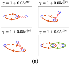
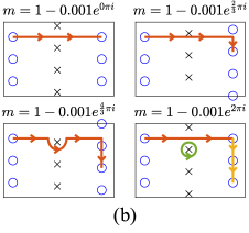
Figure 1: The deformation of the integration path of the instanton action on the Riemann surface of $\sqrt{2V}$ by the monodromy of the deformation parameters around the critical values, (a) for the deformed anharmonic potential (Eq. (5)), and (b) for the Jacobi SD elliptic potential (Eq. (16)). In both cases, the monodromy results in the addition of a residue term (green integration paths) to the instanton action.

This potential reduces to the double-well potential for $\gamma=1$, for which a P/NP relation of the form in Eq. (1) holds [7, 9]. However, for arbitrary values of $\gamma$, modifications to the P/NP relation are necessary to account for the non-vanishing residue. To understand the nature of this modification, notice that for values of $\gamma$ close to $1$, if $\gamma$ is rotated around $1$ by the deformation

$$\gamma\rightarrow 1+(\gamma-1)e^{2\pi i}\,,$$ (8)

the instanton action changes as

$$S(\gamma)\rightarrow S(\gamma)+2\pi R(\gamma)\,,$$ (9)

due to the crossing of a branch cut of the logarithm function appearing in the expression for the instanton action. The monodromic deformations of all such deformed genus-1 potentials result in the addition of a residue term to the instanton action (see Figure (1)).

Inspired by these considerations, we propose that the P/NP relation applicable to deformed genus-1 potentials should also be of the linear form similar to Eq. (1) and should be invariant under the monodromy of the potential. Therefore, proposing an Ansatz for the P/NP relation of the form

$$\frac{\partial E}{\partial B}=-g\left[f(\eta)\,B+g(\eta)\,g\,\frac{\partial A}{\partial g}+h(\eta)\,\frac{\partial A}{\partial\eta}\right]\,,$$ (10)

one finds that to zeroth order in $g$, this equation becomes

$$g(\eta)S(\eta)-h(\eta)\derivative{S(\eta)}{\eta}=1\,.$$ (11)

From the invariance under the monodromy ($S\rightarrow S+2\pi R$), one also finds that the coefficients $g(\eta)$ and $h(\eta)$ of this equation must satisfy

$$g(\eta)R(\eta)-h(\eta)\derivative{R(\eta)}{\eta}=0\,.$$ (12)

From these two equations, one can solve for $g(\eta)$ and $h(\eta)$ and obtain Eq. (3) by changing variables from $\eta$ to $R$.

This relation is also invariant under the addition of a residue term to the instanton function $A$ because the instanton function $A$ also has the same monodromy property as the instanton action. Under the monodromy of the deformation parameter, $A$ shifts by a term proportional to the quantum residue:

$$A(g,B,\eta)\rightarrow A(g,B,\eta)+2\pi\widetilde{R}_{q}(g,\eta)\,.$$ (13)

Nevertheless, the monodromy arguments are not sufficient to reveal the form of Eq. (2), as it encapsulates more information than the Eq. (3), which only relates the instanton function $A$ to the perturbative series $E$. Instead, the relation actually relates $E$ to the quantum period $\mathcal{A}$, the relation of which to the instanton function $A$ is [3, 22]

$$\mathcal{A}(B,g,R)=A(B,g,R)+a_{1}(R)B+B\log(gB)\\ +\sum_{k=2}^{\infty}\frac{B_{k}(1/2)}{k(k-1)}B^{1-k}$$ (14)

where $B_{k}(x)$ are the Bernoulli polynomials. Here, $a_{1}(R)$ is the important term as it depends on $R$. It is the coefficient of the $E^{1}g^{0}$ term in the series expansion of $\mathcal{A}$, and therefore is also the coefficient of the term proportional to $B$, and is chosen such that $A$ has no term of order $g^{0}$. We find that replacing $A$ by $\mathcal{A}$ exactly cancels the function $f(R)$ appearing in Eq. (3), which is a factor that is independent of the instanton function $A$ and is given by

$$f(R)=\frac{1+R\derivative*{a_{1}(R)}{R}}{S(R)-R\derivative*{S(R)}{R}}\,.$$ (15)

Since the instanton function $A$ is defined to have no term of order $g^{0}$, $f(R)B$ is precisely equal to the coefficient of the $g^{1}$ term in $-\partialderivative*{E}{B}$. In practical calculations, it was previously thought that the $+B$ term in Eq. (1) was there only to compensate for the nonexistent $g^{0}$ term in $A$, and that the $g^{1}$ term in $\partialderivative*{E}{B}$ did not affect $A$. But in the P/NP relation in Eq. (2), it becomes clear that the $g^{1}$ term in $\partialderivative*{E}{B}$ in fact determines the $B^{1}g^{0}$ term in the quantum period $\mathcal{A}$ through the relation for $f(R)$ given in Eq. (15), which we have verified for the potentials of our interest.

We stress that the P/NP relation stated in Eq. (3) is a first-order linear partial differential equation and typically requires assigning an initial or boundary value to get a unique solution. Specifically, the solution $A(B,g,\eta)$ is unique only up to some function of the scaled residue, $F(R/g)$. Therefore, to $n$’th order in $g$, the solution $A(B,g,\eta)$ is unique only up to $R^{-n}$, the coefficient of which can be determined without any additional knowledge only under some specific conditions, see App. B for details. If the P/NP relation can be solved uniquely, the non-perturbative function $A$ can be generated solely based on the perturbative function $B$. Conversely, if an initial or boundary value is necessary for the P/NP relationship, one needs to evaluate the non-perturbative function $A$ for a specific value of the deformation parameter, after which equation Eq. (3) can be applied to extend the results to the entire range of the deformation parameter. We will illustrate both cases in the next section.

III Examples

We provide two examples to illustrate the applicability of our P/NP relation in Eq. (3). The first one is the deformed anharmonic potential given in Eq. (5), and the second one is the doubly periodic Jacobi elliptic potential

$$V_{\text{sd}^{2}}(x,m)=\frac{1}{2}\text{sd}^{2}(x,m).$$ (16)

The non-perturbative phenomena appearing in these two examples are, on the surface, completely different. For the deformed anharmonic potential, either real or complex instantons can be in effect depending on the value of the deformation parameter $\gamma$. For the elliptic potential, it is known [29] that, except at the extreme values of $m$, both real and ghost (complex instantons with negative-valued actions) instantons must be simultaneously taken into account, and they both simultaneously govern the large-order behavior of the perturbative expansion for the energy levels. Although these two phenomena are seemingly unrelated, the genus-1 topology of both systems allows them to be united under a common P/NP formula, Eq. (3).

We have already investigated the P/NP relation and the large-order corrections for the deformed anharmonic potential in Eq. (5) in an earlier work [22]. We showed that the P/NP relation for this potential must be modified as

$$\frac{\partial E}{\partial B}=-\frac{3}{2}g\left[\left(5\gamma^{2}-1\right)B+\left(3\gamma^{2}-1\right)g\frac{\partial A}{\partial g}\right.\\ \left.+\left(\gamma^{2}-1\right)\gamma\frac{\partial A}{\partial\gamma}\right]\,.$$ (17)

In light of the P/NP relation in Eq. (3) and the discussion in the previous section, we now understand that Eq. (17) can easily be derived from Eq. (3) by a simple change of variables and noting the instanton action and the residue in Eqs. (6-7). For this potential, the boundary condition for solving the P/NP relation can be fixed uniquely by considering the critical values of the deformation parameter, which was explained in the appendix of [22].

The P/NP relation for the elliptic potential can also be similarly derived. For this potential, the instanton action and the residue read

$$S_{\text{sd}^{2}}(m)=\frac{2\sin^{-1}(\sqrt{m})}{\sqrt{(1-m)m}}\,,\quad R_{\text{sd}^{2}}(m)=\frac{1}{\sqrt{(1-m)m}}$$ (18)

Based on the discussion above, then, the P/NP relation for $V_{\text{sd}^{2}}(x;m)$ can be written as

$$\frac{\partial E_{\text{sd}^{2}}}{\partial B}=-g\left[\frac{1-2m}{2}B+\frac{1-2m}{2}g\frac{\partial A_{\text{sd}^{2}}}{\partial g}\right.\\ \left.-\left(1-m\right)m\frac{\partial A_{\text{sd}^{2}}}{\partial m}\right]\,,$$ (19)

which reproduces the P/NP relation for Sine-Gordon [9, 10] at $m=0$ and the P/NP relation of the Sinh-Gordon potential at $m=1$ . Nevertheless, it should be noted that the boundary condition necessary for solving for $A$ cannot be obtained by considering the critical values $m=0$ or $m=1$ because $R^{-n}=0$ for these values, see App. B for details.

Both examples demonstrate the remarkable link between the perturbative expansion around the perturbative saddle and the instanton function $A$, which encodes the single instanton contribution with fluctuations around them. More precisely, the local information generated around the perturbative saddle through perturbation theory together with a boundary condition is sufficient to construct the non-perturbative instanton function $A$ both for the deformed anharmonic potential and the Jacobi elliptic potential, regardless of the value of the deformation parameter.

Additionally, we demonstrate that the Lamé potential also satisfies our P/NP relation, see App. A for details.

IV Large-order corrections for the elliptic potential

It is well-known in the literature that perturbation theory is divergent and grows factorially in the presence of non-perturbative contributions [1, 2]. In this section, we will validate our P/NP relation given in Eq. (19) by investigating the large-order behavior of the perturbative series for the energy levels of the Jacobi SD potential. The energy $E$ and the instanton function $A$ for this potential are calculated as

$$E_{\text{sd}^{2}}(B,g;m)= B-g\left(\frac{1}{16}-\frac{m}{8}+B^{2}\left(\frac{1}{4}-\frac{m}{2}\right)\right)-g^{2}\left(B\left(\frac{3}{64}+\frac{m}{8}-\frac{m^{2}}{8}\right)+\frac{1}{16}B^{3}\right)$$

$$-g^{3}\left(\frac{9}{2048}-\frac{9m}{1024}+B^{2}\left(\frac{17}{256}-\frac{17m}{128}\right)+B^{4}\left(\frac{5}{128}-\frac{5m}{64}\right)\right)+\mathcal{O}(g^{4})\,,$$ (20)

$$A_{\text{sd}^{2}}(B,g;m) =\frac{S_{\text{sd}^{2}}(m)}{g}+g\left(\frac{3}{32}-\frac{3m}{16}-\frac{1}{4}\sqrt{m-m^{2}}\sin^{-1}\left(\sqrt{m}\right)+B^{2}\left(\frac{3}{8}-\frac{3m}{4}\right)\right)$$

$$+g^{2}\left(B\left(\frac{17}{128}-\frac{5m}{96}+\frac{5m^{2}}{96}\right)+B^{3}\left(\frac{5}{32}-\frac{7m}{24}+\frac{7m^{2}}{24}\right)\right)+\mathcal{O}(g^{3})\,,$$ (21)

which we obtained by solving the Picard-Fuchs equation and calculating the quantum corrections [25, 26, 27, 22]. It can easily be checked that these functions satisfy the P/NP relation in Eq. (19).

To leading order, the prediction of resurgence theory for the large-order behavior of the perturbative series for the energy levels was investigated in [29]. It was shown that the self-duality property of the Jacobi SD function

$$\text{sd}(x,m)=i\,\text{sd}(ix,1-m)$$ (22)

enforces one to include the effects of both real and ghost instantons in the large-order prediction of the energy perturbative series because the self-duality mapping swaps the real and ghost instantons. For the Jacobi SD elliptic potential (16), the ghost instanton action is given by

$$S_{\mathcal{G}}(m)=-S_{\text{sd}^{2}}(1-m)=-\frac{2\sin^{-1}(\sqrt{1-m})}{\sqrt{(1-m)m}}\,,$$ (23)

and the instanton/anti-instanton actions are given by

$$S_{\mathcal{I}\bar{\mathcal{I}}}(m) =2S_{\text{sd}^{2}}(m)\,,$$ (24)

$$S_{\mathcal{G}\bar{\mathcal{G}}}(m) =-2S_{\text{sd}^{2}}(1-m)\,.$$ (25)

We recognize that these two actions differ by a multiple of the residue:

$$S_{\mathcal{G}\bar{\mathcal{G}}}(m)=S_{\mathcal{I}\bar{\mathcal{I}}}(m)-2\pi R_{\text{sd}^{2}}(m)\,.$$ (26)

The reason is that these two instanton/anti-instanton actions are integrals over curves on the Riemann surface of $\sqrt{2V}$, which is effectively a genus-0 surface. Therefore, the only non-zero period of $\sqrt{2V}$ is the residue, and integrals over curves with common start and end points can only differ by the residue.

From the self-duality considerations, the large orders of the perturbative series for the ground state energy grow to leading order as [29]

$$a_{n}^{\text{(leading)}}=-\frac{8n!}{\pi}\left(\frac{1}{(S_{\mathcal{I}\bar{\mathcal{I}}})^{n+1}}-\frac{1}{(S_{\mathcal{G}\bar{\mathcal{G}}})^{n+1}}\right)\,.$$ (27)

This large-order prediction is only up to the leading order, whereas the sub-leading orders of the large-order behavior are governed by the low orders of the instanton function $A$. We will explicitly derive the large-order correction terms solely from the function $A$ in the following.

The self-duality of the Jacobi SD function manifests itself as the invariance of the perturbative series of the energy and the P/NP relation under the mappings $m\rightarrow 1-m$ and $g\rightarrow-g$:

$$E_{\text{sd}^{2}}(B,g;m)=E_{\text{sd}^{2}}(B,-g;1-m)$$ (28)

but the instanton function $A_{\text{sd}^{2}}$ changes under the same mapping. The reason is that the instanton function depends on whether the period in consideration behind it is the real or the ghost period corresponding to the real or ghost instanton. Therefore, we actually have two different instanton functions, which we will call the real and ghost instanton functions.

We define

$$A_{\mathcal{I}\bar{\mathcal{I}}}(B,g,m) =2A_{\text{sd}^{2}}(B,g,m)\,,$$ (29)

$$A_{\mathcal{G}\bar{\mathcal{G}}}(B,g,m) =2A_{\text{sd}^{2}}(B,-g,1-m)$$ (30)

as the real and ghost instanton/anti-instanton functions. These two functions correspond to periods on the WKB curve and can only differ by the quantum residue of the WKB curve:

$$A_{\mathcal{G}\bar{\mathcal{G}}}(B,g,m)=A_{\mathcal{I}\bar{\mathcal{I}}}(B,g,m)-2\pi\widetilde{R}_{q}(g,m)\,,$$ (31)

where the quantum residue is given by Eq. (4). Since the instanton function is expressed as a series in $g$, the quantum residue should also be expanded into a series

$$\widetilde{R}_{q}=\frac{R}{g}-\frac{g}{8R}-\frac{g^{3}}{128R^{3}}-\frac{g^{5}}{1024R^{5}}+\dots\,.$$ (32)

Due to these considerations, having two different $A$ functions does not invalidate the P/NP relation. Since the two functions differ only by a term proportional to the quantum residue, which is a function of the scaled residue $\widetilde{R}=R/g$ only, they both satisfy the P/NP relation because the P/NP relation is invariant under the shift of $A$ by the quantum residue, as explained before.

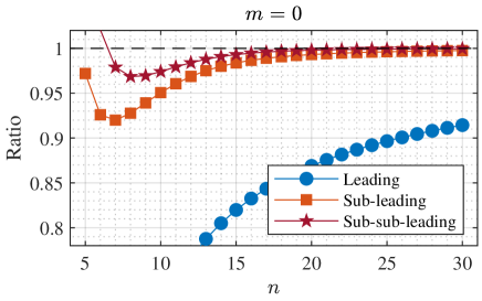
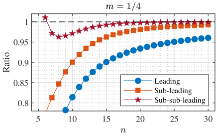
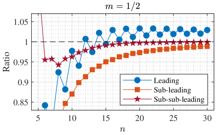
Figure 2: The ratios of the exact coefficients of the perturbative expansion and the large-order growth of the perturbative coefficients for the Jacobi SD potential, $V=1/2\,\text{sd}^{2}(x,m)$, plotted for $m=0$, $1/4$, and $1/2$. The large-order growths are corrected for the leading, sub-leading, and sub-sub-leading predictions by considering the instanton function $A$ up to order $g^{0}$, $g^{1}$, and $g^{2}$, respectively. For $m=1/2$, the odd coefficients in $n$ vanish, but the limit of the ratios as $m\rightarrow 1/2$ exists, which are the values plotted for odd $n$ in the plot for $m=1/2$. The plots for $m$ and $1-m$ are identical due to the self-duality of the Jacobi SD function.

We are now ready to calculate the sub-leading corrections to the large-order behavior of the energy perturbative series. The large-order behavior is directly related to the coefficients of the so-called fluctuation factor. In our case, we have two different fluctuation factors corresponding to the real and ghost instantons. The real fluctuation factor is calculated with the real instanton/anti-instanton action and function

$$F_{\mathcal{I}\bar{\mathcal{I}}}(B,g,m)=\text{exp}\left[-A_{\mathcal{I}\bar{\mathcal{I}}}(B,g,m)+\frac{S_{\mathcal{I}\bar{\mathcal{I}}}(m)}{g}\right]$$

$$\times\frac{\partial E(B,g,m)}{\partial B}$$ (33)

and the ghost fluctuation factor can be calculated by taking the dual of the real fluctuation factor:

$$F_{\mathcal{G}\bar{\mathcal{G}}}(B,g,m)=F_{\mathcal{I}\bar{\mathcal{I}}}(B,-g,1-m).$$ (34)

Then, the large-order prediction with corrections coming from the fluctuation factors is given by

$$a_{n}=- \frac{8n!}{\pi}\left[\frac{1}{(S_{\mathcal{I}\bar{\mathcal{I}}})^{n+1}}\left(1+\frac{b^{\mathcal{I}\bar{\mathcal{I}}}_{1}\,S_{\mathcal{I}\bar{\mathcal{I}}}}{n}+\frac{b^{\mathcal{I}\bar{\mathcal{I}}}_{2}\,S_{\mathcal{I}\bar{\mathcal{I}}}^{2}}{n(n-1)}+\dots\right)\right.$$

$$-\left.\frac{1}{(S_{\mathcal{G}\bar{\mathcal{G}}})^{n+1}}\left(1+\frac{b^{\mathcal{G}\bar{\mathcal{G}}}_{1}\,S_{\mathcal{G}\bar{\mathcal{G}}}}{n}+\frac{b^{\mathcal{G}\bar{\mathcal{G}}}_{2}\,S_{\mathcal{G}\bar{\mathcal{G}}}^{2}}{n(n-1)}+\dots\right)\right]$$ (35)

where the coefficients $b^{\mathcal{I}\bar{\mathcal{I}}}_{n}$ and $b^{\mathcal{G}\bar{\mathcal{G}}}_{n}$ represent the coefficients of $g^{n}$ in $F_{\mathcal{I}\bar{\mathcal{I}}}(B,g,m)$ and $F_{\mathcal{G}\bar{\mathcal{G}}}(B,g,m)$, respectively, for the ground state $B=1/2$.

Figure (2) shows the impact of the fluctuation terms on the large-order factorial growth of the perturbative series for the ground state. The significance of including ghost instantons in the large-order growth of the perturbative series was shown in [29] to leading order. In this work, we demonstrate for the first time that the prediction of large-order terms can be improved further by including the fluctuation terms computed in Eq. (IV). We provide examples for three values of $m$, namely $0$, $1/4$, and $1/2$, and analyze the ratio between the exact coefficients calculated with [31] and the predicted outcomes. In all three cases, adding each correction term further flattens the curve and increases the ratio’s convergence to 1. These results extend symmetrically to $m>1/2$ due to the self-duality of the potential.

The Jacobi SD elliptic potential considered here represents a concrete expression of the idea of resurgence: the perturbative expansion around the perturbative saddle encodes a wealth of information about the non-perturbative saddles. Complex or negatively valued instanton actions should not be dismissed in the analysis of semi-classical expansion as they ultimately play a role in the large-order growth of the perturbative saddle. The validity of Eq. (1) is restricted to systems with vanishing residues only. The P/NP relation in Eq. (3) generalizes this assumption by considering the possibility of non-zero residues, which need to be incorporated into the P/NP relation.

Appendix A P/NP relation for the Lamé equation

The Lamé equation written in the Jacobian form is given by [32]

$$\derivative[2]{w}{z}+\left(h-\nu\left(\nu+1\right)m\,\text{sn}^{2}(z,m)\right)w=0,$$ (36)

which can be converted to a Schrödinger equation

$$-\derivative[2]{\psi}{x}+\frac{1}{2g}\text{sn}^{2}(\sqrt{g}x,m)\psi=E\psi\,,$$ (37)

by the identifications

$$g\rightarrow\frac{1}{\sqrt{2m\nu(\nu+1)}}\,,\quad E\rightarrow\frac{h}{\sqrt{2m\nu(\nu+1)}}.$$ (38)

Therefore, the Lamé equation can be studied as a quantum mechanical system with the potential $V_{\text{Lam\'{e}}}(x,m)=1/2\,\text{sn}^{2}(x,m)$. For the Lamé potential, the instanton action and the residue then read

$$S_{\text{Lam\'{e}}}(m)=\frac{2\tanh^{-1}(\sqrt{m})}{\sqrt{m}}\,,\quad R_{\text{Lam\'{e}}}(m)=\frac{i}{\sqrt{m}}$$ (39)

and one obtains

$$\frac{\partial E_{\text{Lam\'{e}}}}{\partial B}=-g\left[\frac{1+m}{2}B+\frac{1-m}{2}g\frac{\partial A_{\text{Lam\'{e}}}}{\partial g}-\left(1-m\right)m\frac{\partial A_{\text{Lam\'{e}}}}{\partial m}\right]\,.$$ (40)

The energy levels and the instanton function for the Lamé potential are given by

$$E_{\text{Lam\'{e}}}(B,g;m) =B-g\left(\frac{1}{16}+\frac{m}{16}+B^{2}\left(\frac{1}{4}+\frac{m}{4}\right)\right)-g^{2}\left(B\left(\frac{3}{64}-\frac{7m}{32}+\frac{3m^{2}}{64}\right)+B^{3}\left(\frac{1}{16}-\frac{m}{8}+\frac{m^{2}}{16}\right)\right)$$

$$-g^{3}\left(\frac{9}{2048}+\frac{17}{256}B^{2}+\frac{5}{128}B^{4}\right)\left(1-m-m^{2}+m^{3}\right)+\mathcal{O}(g^{4})$$ (41)

$$A_{\text{Lam\'{e}}}(B,g;m) =\frac{S_{\text{Lam\'{e}}}(m)}{g}+g\left(\frac{3}{32}+\frac{3m}{32}+\frac{1}{4}\sqrt{m}\tanh^{-1}\left(\sqrt{m}\right)+B^{2}\left(\frac{3}{8}+\frac{3m}{8}\right)\right)$$

$$+g^{2}\left(B\left(\frac{17}{128}-\frac{41m}{192}+\frac{17m^{2}}{128}\right)+B^{3}\left(\frac{5}{32}-\frac{m}{48}+\frac{5m^{2}}{32}\right)\right)+\mathcal{O}(g^{3})\,,$$ (42)

and they indeed satisfy Eq. (40)

Appendix B General solution of the P/NP relation

Here, we explain how to solve the P/NP relation in the form of Eq. (10), given the information of $E(B,g,\eta)$. It is already known that $A(B,g,\eta)$ must be of the form

$$A(B,g,\eta)=\frac{S(\eta)}{g}+\sum_{n=1}^{\infty}g^{n}\phi_{n}(B,\eta),$$ (43)

and substituting this into Eq. (10), to order $g^{n+1}$, we find

$$n\,g(\eta)\,\phi_{n}(B,\eta)+h(\eta)\partialderivative{\phi_{n}(B,\eta)}{\eta}=-\psi_{n+1}(B,\eta),$$ (44)

where $\psi_{n}(B,\eta)$ is the coefficient of the $g^{n}$ term in $\partialderivative*{E}{B}$. This equation is an inhomogeneous linear differential equation. Using Eq. (12), it can be easily checked that the homogeneous solution is

$$\phi_{n}^{\text{(hom.)}}(\eta)=R(\eta)^{-n}.$$ (45)

The inhomogeneous solution can be found by rewriting the equation in terms of $\varphi_{n}(B,\eta)=R(\eta)^{n}\phi_{n}(B,\eta)$ as

$$h(\eta)R(\eta)^{-n}\partialderivative{\varphi_{n}(B,\eta)}{\eta}=-\psi_{n+1}(B,\eta),$$ (46)

and integrating:

$$\phi_{n}^{\text{(inhom.)}}(B,\eta)=-R(\eta)^{-n}\int\frac{R(\eta)^{n}}{h(\eta)}\psi_{n+1}(B,\eta)\differential{\eta}.$$ (47)

Therefore, the general solution for the coefficients $\phi_{n}(B,\eta)$ is

$$\phi_{n}(B,\eta)=\phi_{n}^{\text{(inhom.)}}(B,\eta)+c_{n}(B)R(\eta)^{-n}.$$ (48)

To have a complete solution for $A(B,g,\eta)$ solely from the knowledge of $E(B,g,\eta)$, $R(\eta)$, and $S(\eta)$, the coefficients of the homogeneous solution, $c_{n}(B)$, must be determined. In the general theory of differential equations, the standard method of determining these coefficients is to provide a boundary condition, specifically, it is necessary to know the solution for $A(B,g,\eta)$ for one specific value of the deformation parameter $\eta$, for which the residue must be finite to have non-vanishing $R^{-n}$.

In the case of the deformed anharmonic potential in Eq. (5), for which we gave the solution in [22], considering the instanton function $A$ for $\gamma=0$ led us to the boundary condition necessary for solving $A$ for any value of the deformation parameter $\gamma$. Since $R(\gamma=0)=0$, $R^{-n}$ blows up at $\gamma=0$. Furthermore, since $\gamma=0$ is not a critical value for the genus-1 curve corresponding to the classical momentum (i.e., the topology of the Riemann surface does not change at $\gamma=0$), $A(B,g,\gamma)$ must be continuous at $\gamma=0$. From both considerations, it was found that $c_{n}(B)=0$ for all $n$ such that $A(B,g,\gamma)$ has a finite expression at $\gamma=0$.

On the other hand, such considerations are not useful in the solution of $A(B,g,m)$ for the Jacobi SD elliptic potential in Eq. (16). For this potential, the only specific values of $m$ that we can use are $m=0$ and $m=1$, but for both values of $m$, $R(m)^{-n}=0$ for $n\geq 1$. Therefore, it is not possible to determine the coefficients $c_{n}(B)$ by having the information of $A$ at $m=0$ and $m=1$. Self-duality considerations (Eqs. (29-31)) can be applied to determine $c_{n}(B)$ for odd $n$, but the coefficients for even values of $n$ remain undetermined.

References

- [1] Carl M. Bender and Tai Tsun Wu. Anharmonic oscillator. Phys. Rev., 184:1231–1260, 1969.
- [2] Carl M. Bender and T. T. Wu. Anharmonic oscillator. 2: A Study of perturbation theory in large order. Phys. Rev. D, 7:1620–1636, 1973.
- [3] Jean Zinn-Justin and Ulrich D. Jentschura. Multi-instantons and exact results I: Conjectures, WKB expansions, and instanton interactions. Annals Phys., 313:197–267, 2004.
- [4] Jean Zinn-Justin and Ulrich D. Jentschura. Multi-instantons and exact results II: Specific cases, higher-order effects, and numerical calculations. Annals Phys., 313:269–325, 2004.
- [5] Ulrich D. Jentschura, Andrey Surzhykov, and Jean Zinn-Justin. Multi-instantons and exact results. III: Unification of even and odd anharmonic oscillators. Annals Phys., 325:1135–1172, 2010.
- [6] Gabriel Álvarez and Carmen Casares. Exponentially small corrections in the asymptotic expansion of the eigenvalues of the cubic anharmonic oscillator. J. Phys. A: Math. Gen., 33(29):5171, 2000.
- [7] Gabriel Álvarez. Langer–Cherry derivation of the multi-instanton expansion for the symmetric double well. J. Math. Phys., 45(8):3095–3108, 07 2004.
- [8] In this context, by the genus of a potential we mean the genus of the Riemann surface of the classical momentum of a particle in that potential.
- [9] Gerald V. Dunne and Mithat Ünsal. Generating nonperturbative physics from perturbation theory. Phys. Rev. D, 89(4):041701, 2014.
- [10] Gerald V. Dunne and Mithat Ünsal. Uniform WKB, multi-instantons, and resurgent trans-series. Phys. Rev. D, 89(10):105009, 2014.
- [11] Gerald V. Dunne and Mithat Ünsal. WKB and resurgence in the Mathieu equation. In Frédéric Fauvet, Dominique Manchon, Stefano Marmi, and David Sauzin, editors, Resurgence, Physics and Numbers, pages 249–298, Pisa, 2017. Scuola Normale Superiore.
- [12] Gerald V. Dunne and Mithat Ünsal. Deconstructing zero: resurgence, supersymmetry and complex saddles. J. High Energy Phys., 2016(12):2, 2016.
- [13] Equivalently, the P/NP relation of the form Eq. (1) only holds for genus-1 potentials for which the Picard-Fuchs equation satisfied by the classical periods reduces to a second-order equation [20, 22] because the residues of must also satisfy the Picard-Fuchs equation.
- [14] Ilmar Gahramanov and Kemal Tezgin. Remark on the Dunne-Ünsal relation in exact semiclassics. Phys. Rev. D, 93(6):065037, 2016.
- [15] A. Gorsky and A. Milekhin. RG-Whitham dynamics and complex Hamiltonian systems. Nucl. Phys. B, 895:33–63, 2015.
- [16] Ilmar Gahramanov and Kemal Tezgin. A resurgence analysis for cubic and quartic anharmonic potentials. Int. J. Mod. Phys. A, 32(05):1750033, 2017.
- [17] Gökçe Başar and Gerald V. Dunne. Resurgence and the Nekrasov-Shatashvili limit: connecting weak and strong coupling in the Mathieu and Lamé systems. J. High Energy Phys., 2015(2):160, 2015.
- [18] Can Kozçaz, Tin Sulejmanpasic, Yuya Tanizaki, and Mithat Ünsal. Cheshire Cat Resurgence, Self-Resurgence and Quasi-Exact Solvable Systems. Commun. Math. Phys., 364(3):835–878, 2018.
- [19] Santiago Codesido and Marcos Marino. Holomorphic anomaly and quantum mechanics. J. Phys. A: Math. Theor., 51(5):055402, 2018.
- [20] Gökçe Başar, Gerald V. Dunne, and Mithat Ünsal. Quantum geometry of resurgent perturbative/nonperturbative relations. J. High Energy Phys., 2017(5):87, 2017.
- [21] Alexander van Spaendonck and Marcel Vonk. Exact instanton transseries for quantum mechanics. SciPost Phys., 16(4):103, 2024.
- [22] Atakan Çavuşoğlu, Can Kozçaz, and Kemal Tezgin. Unified genus-1 potential and parametric P/NP relation. 11 2023.
- [23] The scaled instanton action and residue appear more fundamentally in the P/NP relation because they are the quantities corresponding to the potential scaled by the coupling constant, i.e., to the potential .
- [24] A. Voros. The return of the quartic oscillator. The complex WKB method. Annales de l’I.H.P. Physique théorique, 39(3):211–338, 1983.
- [25] A. Mironov and A. Morozov. Nekrasov functions and exact Bohr-Sommerfeld integrals. J. High Energy Phys., 2010(4):40, 2010.
- [26] Fabian Fischbach, Albrecht Klemm, and Christoph Nega. WKB method and quantum periods beyond genus one. J. Phys. A: Math. Theor., 52(7):075402, 2019.
- [27] Michael Kreshchuk and Tobias Gulden. The Picard–Fuchs equation in classical and quantum physics: application to higher-order WKB method. J. Phys. A: Math. Theor., 52(15):155301, 2019.
- [28] Eric Delabaere, Hervé Dillinger, and Frédéric Pham. Exact semiclassical expansions for one-dimensional quantum oscillators. J. Math. Phys., 38(12):6126–6184, 12 1997.
- [29] Gökçe Başar, Gerald V. Dunne, and Mithat Ünsal. Resurgence theory, ghost-instantons, and analytic continuation of path integrals. J. High Energy Phys., 2013(10):41, 2013.
- [30] It should be noted that this reduction is not apparent in the expression for the residue, which blows up at or . The reason is that the pole structure of the elliptic potential on the complex plane changes specifically at or . For other values of , the elliptic potential is doubly periodic and has infinitely many poles on the complex plane, one in each fundamental lattice. But for or , the potential becomes periodic in one direction only, the only remaining pole being at infinity with zero residue. Therefore, the expression for the residue in terms of is not valid for or .
- [31] Tin Sulejmanpasic and Mithat Ünsal. Aspects of perturbation theory in quantum mechanics: The BenderWu Mathematica ® package. Comput. Phys. Commun., 228:273–289, 2018.
- [32] NIST Digital Library of Mathematical Functions. https://dlmf.nist.gov/29.2. Accessed: 2024-04-28.