Fairness in Multi-Proposer-Multi-Responder Ultimatum Game

Abstract

The Ultimatum Game is conventionally formulated in the context of two players. Nonetheless, real-life scenarios often entail community interactions among numerous individuals. To address this, we introduce an extended version of the Ultimatum Game, called the Multi-Proposer-Multi-Responder Ultimatum Game. In this model, multiple responders and proposers simultaneously interact in a one-shot game, introducing competition both within proposers and within responders. We derive subgame-perfect Nash equilibria for all scenarios and explore how these non-trivial values might provide insight into proposal and rejection behavior experimentally observed in the context of one vs. one Ultimatum Game scenarios. Additionally, by considering the asymptotic numbers of players, we propose two potential estimates for a ”fair” threshold: either 31.8% or 36.8% of the pie (share) for the responder.

Introduction

The Ultimatum Game (UG) has been one of the paradigmatic games for studying fairness since its introduction in 1982 by Güth et al. [1]. This simple one-shot game consists of a reward and two players with asymmetric roles: proposer and responder. The proposer’s task is to suggest a split of the reward between the players. The responder can then accept or reject this split. On acceptance, the reward is split accordingly, and on rejection, both players receive nothing. The theoretical prediction states that a rational self-interested proposer will offer the minimum amount they believe the responder will accept. Similarly, a rational self-interested responder will accept any positive offer and remain indifferent between accepting or rejecting a zero offer. Thus, the subgame-perfect Nash equilibrium [2], dictates the proposer to offer the smallest possible unit of the reward which the responder then accepts.

However, in experiments, real-world players do not play as predicted by this theory (see e.g. Camerer [3] and Henrich et al. [4]). In Western, educated, industrialised, rich, democratic (W.E.I.R.D) societies, responders reject offers of less than 20$\%$ of the reward with a probability of one-half and almost always accept proposals of 40$\%$ to 50$\%.$ Proposers’ modal offers are usually between $40\%$ to $50\%$ and mean offers between $30\%$ to $40\%$ [3]. For example, Oosterbeek et al. [5] found in their comprehensive review a mean offer of $40\%.$ On the other hand, experimental results on UG-like scenarios (see again [4]), played in various small-scale societies, report more variable proposer and responder thresholds, ranging from greedy to generous. Interestingly, among the most generous proposers are tribal whaler societies [6], whose lifestyle requires high levels of cooperation and mutual trust. Elsewhere, it is common for low offers to be both proposed and accepted [7, 8].

Additionally, the sensitivity to biases, including anonymity, stake level, and context effects have been studied, and it was concluded they do not seem to shift played thresholds significantly [9, 10, 11]. Moreover, priming players, e.g. by conjuring an imaginary right to play proposer, has been found to make players propose more greedily (see Hoffman et al. [12]), although some of the results have been recently contested by Demiral and Mollerstrom [13]. A concise understanding of how human sharing and cooperation behavior precisely depends on context and circumstances (including the complexity of social interactions in terms of multi-player scenarios) is, therefore, still partly to be found.

Whether fairness is part of our ancestral behavioural makeup that evolved among apes or can be attributed only to the ”modern” self-domesticated human [14, 15] is still debated [16, 17, 18, 19].

W.E.I.R.D. societies have been shown to follow a unique cognitive trajectory, concerning sharing and cooperation, which can be traced back to a change in inheritance law in 305 AD. It was introduced by the Catholic Church due to its preoccupation with incest, promoting heritage by testament, banning polygamous marriages and marriages to relatives, promoting the newlywed to set up independent households [20, 21].

This reform, over a period of more than a thousand years, broke up clan structures and thereby fostered individuality over clan-identity, and the interaction and cooperation of individuals across clan-boundaries, which may explain some peculiarities of the W.E.I.R.D. world. In summary, our evolutionary and societal development remains partly veiled in the dusk of the past and can only be accessible through comparative studies (e.g. [14]) and to a hypothetical realism that largely remains grounded in mathematical modeling.

Evolutionary game theory is a common framework for studying the emergence of fairness (see e.g. Debove et al. [22] who review various evolutionary game-theoretic models of the UG type). For instance, some models on networks indicate a dependence of the proposer and responder thresholds on the topology of the social network (see e.g. Sinatra et al. [23], Kuperman and Risau-Gusman [24] and Page et al. [25]); others explore the role ”social status”, may play [26]. Alternatively, Fehr and Schmidt [27] propose an inequity-aversion framework in their seminal work. Also, see the review by Güth and Kocher [28].

Regarding generalisations of the UG to multiple players, the majority of theoretical and experimental extensions typically focus on scenarios with either one proposer and many responders or vice versa. For instance, Roth et al. [29] conducted experiments with proposer competition and one responder, while Fischbacher et al. [30] explored responder competition. They showed that introducing competition raises the offers in the former and decreases offers in the latter as compared to the one vs. one UG.

Additionally, Santos et al. [31] investigated an evolutionary game-theoretic model with a group decision-making process for responders when faced with an offer from a single proposer. In another paper, Santos and Bloembergen [32] extend the UG to a group of proposers playing with a group of responders. The group of responders rejects the average proposed offer if it is lower than their average group acceptance threshold. In generosity or envy games there is an additional third dummy player that takes no active role (for details see survey from Güth and Kocher [28]).

In this paper, we introduce an extension of the UG where multiple proposers and multiple responders engage in a one-shot interaction. This extended model seems to be more appropriate in various social contexts, such as the tribal whaler society mentioned above than the classical two-player paradigm. It constitutes a two-sided market, where proposers simultaneously make their offers, and responders, in turn, simultaneously each select an offer from one of the proposers (or choose a number with some probability), or decline all offers. If a proposer is chosen by at least one responder, they receive the proposed split. Conversely, if no responders select them, they receive nothing. On the other hand, all responders who chose a proposer that was not selected by anyone else will receive their share. In cases where multiple responders choose the same proposer, only one of them, randomly selected, receives the proposed split, while the other responders receive nothing.

In the context of a simplified labor market, proposers represent potential employers and responders potential employees. We assume that the employers offer identical roles, such as a plumbing job, where the reward is the total revenue, and they must decide how to split it with the employee. If an employer decides to claim too large a share of the revenue, they run the risk of being outbid by other employers and earning nothing. Similarly, if the employees would simply choose the highest offer, they may end up making the same choice as many other responders, resulting in no job opportunity if they are not selected by the probabilistic rule. An essential factor influencing the ”optimal” offers of employers is the balance between the number of available jobs (employers) and the number of potential employees. Alternatively, within a biological context, proposers may symbolise plants, offering their energy in the form of nectar, while responders represent the pollinators.

A similar concept to the multiplayer UG is sequential bargaining (see e.g. Rubinstein and Wolinsky [33], Li et al. [34]). In these models, the proposer role is passed on around players until everyone agrees with the division. In Li et al. [34] they describe a model with two buyers and two sellers. Sequentially, each participant selects a partner from the opposing group and initiates bargaining by making an offer. If the initial pair reaches an agreement, they quit bargaining and leave with their share. However, in the case of rejection, they remain open to being chosen by another seller or buyer for further bargaining. If not all players agree on a share, in the subsequent round the other group takes the role of the proposer and makes the offers. However, these models differ due to their sequential quality and role switching, whereas in our model we present a one-shot model.

This paper is organised as follows. In the following section, we present a formalisation of the game and (for a self-contained description) briefly introduce the subgame-perfect Nash equilibria of the one vs. one and one vs. many UG scenarios. Then, in Two Proposers and Two Responders we provide a detailed analysis of the game involving two proposers and two responders, where we find the subgame-perfect Nash equilibrium of the game. Subsequently, in $K$ Proposers and $L$ Responders, we derive the solution for the general case of multiple proposers facing multiple responders. In the Discussion we scrutinise the discovered solutions, look closer at their asymptotic properties, and discuss some implications for fairness in human behaviour. Lastly, we summarise our results in the Conclusions.

The Model

In the following we extend the framework of the classical UG to a Multi-Proposer-Multi-Responder (MPMR) framework and, at the same time, comment on known results of three special cases: one responder vs. one proposer, many responders vs. one proposer, and one responder vs. many proposers.

The MPMR UG game involves $L\in\mathbb{N}$ responders and $K\in\mathbb{N}$ proposers. Each proposer is endowed with a potential reward of size one that is to be split with one of the responders. The game has two stages. In the first stage, each proposer puts forward a split of the reward denoted as $s_{i}\in[0,1]$, where ${i\in\{1,2,\dots,K\}}$, offering $s_{i}$ to the responders and ${1-s_{i}}$ to themselves. In the second stage of the game, responders simultaneously and independently (without the knowledge of other responders’ choices) select one of the proposers or select no one. Additionally, they may also use mixed strategies and probabilistically decide between multiple proposers. Responders have full information about all the proposed offers and are impartial towards the proposers themselves. Following the decision of the responders, the payoffs are distributed. If the proposer $i$ was selected by at least one responder, they receive $1-s_{i}$, otherwise, they receive nothing. Similarly, only one responder picked randomly (with probability one divided by the number of individuals that chose the same proposer) among the respective responders receives the offered split $s_{i}$, the others receive nothing, just as responders who did not choose any proposer would.

Let us rewrite the payoffs in symbolic terms. Denote $N_{R,i}\in\{0,1,\dots,L\},$ $i\in\{1,2,\dots,K\}$ as the number of responders that chose the proposer $i$. The payoff $\pi_{P,i}$ of proposer $i$ with offer $s_{i}\in[0,1]$ is calculated as:

$$\pi_{P,i}=\begin{cases}\begin{aligned} &1-s_{i}&\quad\text{if }&N_{R,i}\geq 1\ ,\\ &0&\quad\text{if }&N_{R,i}=0\ .\end{aligned}\end{cases}$$

The payoff $\pi_{R,j}$ of the responder $j,j\in\{1,2,\dots,L\}$ that chose proposer $i$ is given as

$$\pi_{R,j}=\begin{cases}\begin{aligned} &s_{i}&\quad&\text{with probability }\frac{1}{N_{R,i}}\ ,\\ &0&\quad&\text{with probability }\frac{N_{R,i}-1}{N_{R,i}}\ .\end{aligned}\end{cases}$$

The payoff $\pi_{R,j}$ of the responder $j$ who rejected all offers is given as:

$$\pi_{R,j}=0\ .$$

In Fig. 1 we illustrate the mechanics of the MPMR UG in a simple scenario.

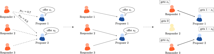
Figure 1: Graphical representation of the game for the case of $L=3$ responders and $K=2$ proposers. In the first stage, proposers announce their offers, prompting each responder to determine their selection strategy. In this scenario, responder $1$ chooses a mixed strategy while the other two responders play pure strategies. In the second stage, it is probabilistically decided that responder $1$ chooses proposer $1$. Since two responders chose proposer $2,$ another probabilistic realisation determines who gets paired with the proposer. In this case, responder $2$ is unpaired, resulting in a zero payoff. Similarly, if one of the proposers (or both) would not be selected they would receive a zero payoff.

Before going into further analysis let us first summarise the known results for three basic cases of the game. With one proposer and one responder, the game reduces to a classical UG. If the responder’s strategy is to refuse any offer other than $s,s\in[0,1]$ then the proposer offering $s$ corresponds to a Nash equilibrium. Likewise, it constitutes a Nash equilibrium if we presume that once a responder accepts $s$, they will accept any offer $s^{*}$ greater than $s.$ Consequently, there exists a continuum of Nash equilibria in the UG. To reduce their number, attention can be directed towards the concept of a subgame-perfect Nash equilibrium [2]. If the proposer deviates from their strategy and offers slightly less than $s$, in this subgame, the responder’s best-reply is to accept the offer. Consequently, no $s>0$ can be a subgame-perfect equilibrium, since the proposer can always improve their payoff by lowering the offer. Thus, there exists a unique subgame-perfect equilibrium where the proposer offers ${s=0}$ and the responder accepts all offers. If there exists a grid of possible offers instead of a continuous interval, the second smallest possible offer $\epsilon>0$ is also a subgame-perfect equilibrium. This is because the responder maximises their payoff regardless of accepting or rejecting the offer of $s=0$ and may choose to reject a zero offer, in which case the proposer’s subgame-perfect equilibrium is to offer $\epsilon.$

Similarly, in the case of multiple responders facing a single proposer, in the subgame-perfect equilibrium responders are offered zero and at least one of them accepts the offer. Once again, in the case of the existence of the second smallest offer, this is a subgame-perfect equilibrium too if all responders reject the zero offer. In the case of proposer competition, where multiple proposers face a single responder, in the subgame-perfect equilibrium at least two proposers offer $s=1$ which the responder accepts (note that the other proposers can offer any split, which subsequently leads to multiple equilibria). For details see e.g. [27].

In the next sections, we will see that the introduction of two-sided competition yields intriguing outcomes. Since only one responder gets their share of the reward if more than one of them select the same proposer, it may not always be optimal for responders to straightforwardly select the best proposal, as others might employ the same approach. Instead, a more efficient strategy might involve granting a non–zero probability of going to the second-best proposal and other alternative offers. In this sense, the two-sided competition problem introduces a minority-game-like situation (as in the El Farol Bar problem [35]) into the MPMR UG scenario. Consequently, the proposers are motivated to make offers below the offer of one, as there is a possibility that the second-best offer might still be accepted by some responder. On the other hand, there is still the presence of competition between the proposers which prevents them from offering zero.

In the next section, we start with the scenario involving two proposers and two responders.

Two Proposers and Two Responders

In this section, we provide an analysis of the MPMR UG with two proposers and two responders. Our goal is to find subgame-perfect Nash equilibria. We will see that in each subgame with at least one positive offer there are either one or two Nash equilibria for the responders, depending on the combination of offers. Only one of them is also an evolutionarily stable strategy (ESS) and when restricting ourselves to that strategy there is a unique subgame-perfect Nash equilibrium where both proposers offer $s=0.5$ and both responders select each of them with probability $0.5.$

Responders’ Nash Equilibrium

Let us start with denoting the strategy of one particular subgame (i.e. how much is offered to the responders) for the first proposer as $s_{1}\in[0,1]$ and for the second proposer as $s_{2}\in[0,1].$ Without loss of generality we assume $s_{1}\leq s_{2}.$ The mixed strategies of the respective responders (denoted $R_{1}$ and $R_{2}$) selecting the respective proposers (denoted $P_{1}$ and $P_{2}$) will be given as:

$$P(R_{1}\text{ choosing }P_{1}) =p,\ P(R_{1}\text{ choosing }P_{2}) =1-p,$$

$$P(R_{2}\text{ choosing }P_{1}) =q,\ P(R_{2}\text{ choosing }P_{2}) =1-q,$$

where $p,q\in[0,1]$ (note neither of the responders rejects any offer since this simplification does not prevent us from finding the best reply strategies). Considering these strategies we can calculate the expected payoffs of responders, denoted by $\Pi_{R,1},\Pi_{R,2}$ for the first and second responder respectively:

$$\Pi_{R,1}(p,q) =s_{1}p\left(1-q+\frac{q}{2}\right)+s_{2}(1-p)\left(q+\frac{1-q}{2}\right),$$

$$\Pi_{R,2}(p,q) =\Pi_{R,1}(q,p)\ .$$

Next, we want to find the best response of the first responder given a set of offers $(s_{1},s_{2})$ and a fixed mixed strategy $(q,1-q)$ of the second responder. We start by finding $p$ that maximises $\Pi_{R,1}.$ Notice the payoff $\Pi_{R,1}$ is linear in $p.$ Thus, the derivative of $\Pi_{R,1}$ with respect to $p$ is constant for all $p$ and given as:

$$\frac{\partial\Pi_{R,1}}{\partial p}=s_{1}-\frac{s_{2}+qs_{1}+qs_{2}}{2}.$$ (1)

It is easy to find the best response strategy of the first responder, denoted by $p^{*}:$

$$p^{*}=\begin{cases}\begin{aligned} &[0,1]\quad&\text{if }s_{1}&=s_{2}=0,\\ &[0,1]\quad&\text{if }q&=q_{\rm{crit}}\equiv\frac{2s_{1}-s_{2}}{s_{1}+s_{2}},\\ &1\quad&\text{if }q&<q_{\rm{crit}},\\ &0\quad&\text{if }q&>q_{\rm{crit}}.\\ \end{aligned}\end{cases}$$ (2)

We would get mirror results for the best response strategy of the second responder since the responder roles are symmetric. It is evident from (2), that when the higher offer $s_{2}$ exceeds twice the value of $s_{1}$, it is advantageous for both responders to disregard the lower offer $s_{1}.$ Conversely, in instances where the offers are sufficiently similar ($s_{2}\leq 2s_{1}$), a critical threshold $q_{\rm{crit}}$ emerges. If the second responder plays the threshold strategy $q_{\rm{crit}}$, the first responder’s strategy becomes irrelevant. If the responder plays a different strategy to $q_{crit},$ the best response is to choose exclusively the other relatively less occupied proposer with respect to the threshold. As a consequence, the Nash equilibrium for responders in the subgame with fixed offers $s_{1}\leq s_{2}$ is:

Sc. 0: if $$s_{1}=s_{2}=0 p_{0},q_{0}\in[0,1]\text{ or reject.}$$ (3)

Sc. A: if $$s_{2}<2s_{1} p_{A}=q_{A}=\frac{2s_{1}-s_{2}}{s_{1}+s_{2}}.$$

Sc. B: if $$s_{2}<2s_{1} p_{B}=0,\hskip 5.0ptq_{B}=1\text{ or reversed.}$$

Sc. C: if $$s_{2}=2s_{1}\neq 0 p_{C}=0,q_{C}\in[0,1]\text{ or reversed.}$$

Sc. D: if $$s_{2}>2s_{1} p_{D}=q_{D}=0.$$

In Scenario 0 both proposers offer zero and responders receive a zero payoff, no matter which strategy they choose. In Scenario D one of the offers is more than double the amount proposed by the other proposer. Thus, both responders opt for the proposer with the higher offer and discard the other. In Scenario C, there is a continuum of Nash equilibria, however, playing the strategy of going to the second proposer with offer $s_{2}$ is a weakly dominant strategy (this is easy to see, since the payoff is given as $\Pi_{R,1}=s_{1}(1+q-\frac{3}{2}pq)$). Notice that when the ratio of the offers is less than two ($s_{2}<2s_{1}$), two types of Nash equilibrium strategies for the responders emerge: symmetric strategies (Scenario A) and strategies which require ”coordination” of the responders (Scenario B). Let us now look closer at how these strategies perform when played against each other. We denote the offer levels as $s_{1}=s,$ where $s\in[0,1]$ and $s_{2}=s+\delta,$ where $0\leq\delta<s$ and $0<s_{2}\leq 1.$ The payoff matrix for responders playing strategies $p_{A},p_{B}$ against $q_{A},q_{B}$ is shown in Table 1.

	$q_{A}$	$q_{B}=0$	$q_{B}=1$
$p_{A}$	$\frac{3s(s+\delta)}{2(2s+\delta)}$	$\frac{3s(s+\delta)+2\delta(\delta-s)}{2(2s+\delta)}$	$\frac{3s(s+\delta)+2\delta(2\delta+s)}{2(2s+\delta)}$
$p_{B}=0$	$\frac{3s(s+\delta)}{2(2s+\delta)}$	$\frac{1}{2}(s+\delta)$	$s+\delta$
$p_{B}=1$	$\frac{3s(s+\delta)}{2(2s+\delta)}$	$s$	$\frac{1}{2}s$

Table 1: Payoff matrix for responders playing strategy $p_{A},p_{B}=1$ and $p_{B}=0$ in Scenario A and Scenario B.

Choosing the lower offer with probability zero ($p_{B}=0$) is the best response against both $q_{A}$ and $q_{B}=1,$ however when played against the same strategy $q_{B}=0$ the strategy is inferior to $p_{A}$ and $p_{B}=0.$ Thus, contrary to Scenario C, there is no weakly dominant strategy. In order to determine which of the two Nash equilibria will be played by the responders, we can turn to the concept of an evolutionarily stable strategy. As we prove in the Supplementary Information (see Theorem 1) the symmetric strategy $p_{A}$ is uniquely evolutionarily stable, which means that it is (in this way) superior to other strategies.

We also explored the replicator dynamics with the co-existence of three types of Nash equilibrium strategies: $\gamma$–players who always choose the strategy of Scenario A, $\alpha$–players who always choose the highest offer and $\beta$–players who always choose the lowest offer. The analysis, detailed in the Supplementary Information, reveals that in the stable state $\alpha$– and $\beta$–players’ relative abundances on average yield the same strategy as the Scenario A strategy, albeit on a population-wide level rather than an individual one. The abundance of $\gamma$–players depends on the initial conditions. Thus, in the next part, we reduce the analysis to responders playing the Nash equilibrium strategy $p_{A}.$

Proposers’ Nash Equilibrium Strategy

In this section, we will derive the subgame-perfect Nash equilibrium of the proposers. Without loss of generality, we assume that $s_{1}\leq s_{2}.$ As demonstrated in the preceding section, in the cases where $2s_{1}\leq s_{2},$ both responders choose the proposer with the higher offer and the other proposer receives no reward. Since the abandoned proposer can improve their payoff by increasing their offer to slightly more than half of the other offer, this situation cannot be a Nash equilibrium. For the case where $s_{1}=s_{2}=0$, there is a subgame-perfect Nash equilibrium. Here both responders receive zero, no matter what their strategy is. If each responder accepts and chooses different proposers, then both proposers receive the maximal payoff of one. However, this requires responders to accept a zero reward and align, i.e. to match their choices and can be considered degenerate. Any other matching (or rejection) does not lead to a subgame-perfect Nash equilibrium. Then one of the proposers (or both) has an expected payoff of less than one and by raising their offer from zero to a sufficiently small offer $\epsilon$, they are able to secure a better payoff, $1-\epsilon$.

In the following, we will only consider offers satisfying ${0<s_{2}\leq 2s_{1}}$. The expected payoffs of proposers $1$ and $2,$ with offers $s_{1}$ and $s_{2}$ respectively (denoted $\Pi_{P,1}$ and $\Pi_{P,2}$ respectively), are:

$$\Pi_{P,1} =(1-s_{1})\left(pq+p(1-q)+q(1-p)\right)\ ,$$ (4)

$$\Pi_{P,2} =(1-s_{2})((1-p)(1-q)+p(1-q)+q(1-p))\ ,$$

where $(p,1-p)$ and $(q,1-q)$ are the responders’ strategies. We assume that the responders choose the strategy $p_{A}$ (see  (3)) according to the Nash equilibrium Scenario A (for reasons why we do not focus on Scenario B strategy see above). Then we can rewrite the expected payoffs as:

$$\Pi_{P,1} =\frac{3s_{2}(2s_{1}-s_{2})(1-s_{1})}{(s_{1}+s_{2})^{2}}\ ,$$ (5)

$$\Pi_{P,2} =\frac{3s_{1}(2s_{2}-s_{1})(1-s_{2})}{(s_{1}+s_{2})^{2}}\ .$$

To maximise the payoffs we set $\partial\Pi_{P,i}/\partial s_{i}=0$, with $i=1,2$, identify the best response of the proposers, yielding for the first and second proposer:

$$s_{1}^{*}=f(s_{2})=\frac{s_{2}^{2}+4s_{2}}{5s_{2}+2}\quad{\rm and}\quad s_{2}^{*}=f(s_{1})=\frac{s_{1}^{2}+4s_{1}}{5s_{1}+2}\ .$$

The subgame-perfect Nash equilibrium $(s_{1}^{*},s_{2}^{*})$ has to satisfy $s_{1}^{*}=f(f(s_{1}^{*}))$ leading to a fourth order polynomial that has four roots $\{0,\frac{1}{2},-3+\sqrt{7},-3-\sqrt{7}\}.$ However, the only physical, non-trivial solution is $\frac{1}{2}$, which leads to the unique non-degenerate Nash equilibrium of symmetric offers $(\frac{1}{2},\frac{1}{2}).$ In that case, the payoffs of the players are the same in both roles:

$$\Pi_{R,1}=\Pi_{R,2}=\Pi_{P,1}=\Pi_{P,2}=\frac{3}{8}\ .$$ (6)

Finally, we remark on a potentially counter-intuitive observation: by changing the rules of the game and giving the responders a chance to coordinate for maximizing their common payoff in each subgame, their subgame-perfect Nash equilibrium payoffs are lower than in the MPMR UG.

It is easy to see this from the following. Opting for the strategy where one responder selects the first proposer while the other selects the second results in the responders receiving all of the available reward in every subgame, so more than with any other strategy. Then, the payoffs of the proposers are:

$$\Pi^{*}_{P,1} =1-s_{1}\ ,\quad\Pi^{*}_{P,2} =1-s_{2}\ .$$ (7)

However, then the subgame-perfect equilibrium is $(0,0)$ and the responders accept, since, under all offer combinations, the proposers receive their offered split and they have no incentive to raise the offers from zero. Thus, this type of coordination leads to worse outcomes for the responders.

K Proposers and L Responders

Now to the general case of $K\in\mathbb{N}$ proposers and $L\in\mathbb{N}$ responders where $K,L\geq 2.$

Responders’ Strategy

Let us find the Nash equilibria for the responders for subgames determined by offers from $K$ proposers. Let $p_{ij}=P(\text{$R_{i}$ choosing $P_{j}$}),$ ${i\in\{1,2,\dots,L\}}$, with $j\in\{1,2,\dots,K\}$, denote the probability of the responder $i$ choosing proposer $j$, who offers $s_{j}\in[0,1].$ Naturally, $\sum_{j=1}^{K}p_{ij}=1$ and $p_{ij}\geq 0$ and the expected payoff $\Pi_{R,l}$ of the responder $l$ is:

$$\Pi_{R,l}=\sum_{i=1}^{K}s_{i}W_{li}\cdot p_{li}\ ,$$

where

$$W_{li}=\sum_{j=1}^{L}\frac{1}{j}\left[\sum_{\alpha:\left\lVert\alpha\right\rVert_{1}=j,\alpha_{l}=1}\prod_{k=1,k\neq l}^{L}p_{ki}^{\alpha_{k}}(1-p_{ki})^{1-\alpha_{k}}\right]\ ,$$

with $\alpha\in\{0,1\}^{L}$ and $\left\lVert.\right\rVert_{1}$ being the $L^{1}$ norm. Each term of the sum in $W_{li}$ describes the probability of precisely $j$ responders (including responder $l$) choosing proposer $i,$ weighted by $\frac{1}{j}.$ Also notice that $W_{li}$ is independent of $p_{li},$ meaning that payoff $\Pi_{R,l}$ is a linear function defined by strategy ${p_{l}=(p_{l1},p_{l2},\dots p_{lK})}$ and scalars $(s_{1}W_{l1},s_{2}W_{l2},\dots,s_{K}W_{lK}).$ In order to find the best response of responder $l$ facing the other responders, we have to solve a constrained optimisation problem on a linear function. Without loss of generality, we set the ordering of proposers to be determined by:

$$s_{K}W_{lK}\geq s_{i}W_{li}\ ,$$

for all $i\in\{1,2,\dots,K\}$ and analyse the derivative of the payoff of responder $l$ with respect to ${p_{li},i\in\{1,\dots,K-1\}}$ where $p_{lK}=1-\sum_{j=1}^{K-1}p_{lj}:$

$$\frac{\partial\Pi_{R,l}}{\partial p_{li}}=s_{i}W_{li}-s_{K}W_{lK}\ .$$ (8)

Thanks to the ordering, we know the derivative ((8)) has only non-positive values. The best response strategy is to set as zero all $p_{li}$ for which $\frac{\partial\Pi_{R,l}}{\partial p_{li}}<0$ and when determining the remaining probabilities where $\frac{\partial\Pi_{R,l}}{\partial p_{li}}=0$ the responder is ambivalent. Translating these best responses to Nash equilibria for each subgame is more intricate in the higher-dimensional scenario than in the simpler two-on-two case.

Once again, there is a Scenario 0-like regime where all proposers offer zero and the responders’ strategy is inconsequential– responders receive zero in all cases. There are also regimes similar to Scenarios C and D where some of the proposers offer too little compared to the other proposers and their offers get discarded by every responder. In regimes where all offers are sufficiently similar to each other, both symmetric and asymmetric Nash equilibria resembling Scenario A and Scenario B can emerge, where each proposer has a positive probability of being selected. As an example, consider the case of two responders and three proposers offering identical offers $s\in(0,1].$ Let $p=(p_{11},p_{12},p_{13})$ and $q=(p_{21},p_{22},p_{23})$ represent the responders’ probabilities for selecting the proposers. Both $p=q=(1/3,1/3,1/3)$ and $p=(1,0,0)$ and $q=(0,x,1-x)$ with $x\in[0,1]$ constitute Nash equilibria. Thus, a continuum of Nash equilibria exists, contrary to the previous section, where only two Nash equilibria emerge in the case of identical offers.

Due to these intricacies, we refrain from explicitly deriving parameter regions and all possible Nash equilibria for the responders. Instead, we restrict our analysis to Nash equilibria for the responders that are evolutionarily stable. For that, we consider an infinite population of responders from which we choose the respective number of players in each subgame. Thus, the players cannot coordinate. In Theorem 2 (see the Supplementary Information, ”General Case”), we prove that for any combination of offers $(s_{1},s_{2},\dots,s_{K})$, apart from purely zero offers ($s_{i}=0,$ for all $i\in\{1,2,\dots,K\}$), there exists a unique evolutionarily stable strategy for the responders. We will consider this responder strategy to be the ”superior” Nash equilibrium, in the sense of evolutionary stability. Now we will show some implicit results about the evolutionarily stable Nash equilibrium.

Without loss of generality, let $s_{K}\geq s_{K-1}\geq\cdots\geq s_{1}$ with $s_{K}>0$ represent the offers from $K\geq 2$ proposers. Assume that all responders employ the evolutionarily stable strategy $\{p_{i}\}_{i=1}^{K}$. When including the same strategy $p_{li}=p_{i}$ for all $l\in\{1,2,\ldots,L\},$ $i\in\{1,2,\dots,K\}$ in the derivative (see (8)), we obtain the same derivative of the payoff for all responders (denoted $\Pi_{R}$):

$$\frac{\partial\Pi_{R}}{\partial p_{i}} =\frac{1}{L}(s_{i}f(p_{i})-s_{K}f(p_{K}))\ ,$$ (9)

where $i\in\{1,2,\dots,K-1\}$ and $f(x)$ is defined as:

$$f:[0,1]\to\mathbb{R}\ ,\quad f(0)=L\ ,$$

$$f(x)=L\sum_{j=1}^{L}\frac{1}{j}{L-1\choose j-1}x^{j-1}(1-x)^{L-j}=\frac{1-(1-x)^{L}}{x}\ .$$

The function $f$ is continuous and strictly decreasing on $[0,1]$ (see Lemma 1 in the Supplementary Information). Since $s_{K}$ is the highest offer, $p_{K}$ has to be greater than zero in the Nash equilibrium, which means no other $p_{i}$ can be equal to one. Therefore, all derivatives must be non-positive in the Nash equilibrium. Then, for the evolutionarily stable strategy $\{p_{i}\}_{i=1}^{K}$ it has to follow for all $i\in\{1,2,\dots,K-1\}$ that:

$$p_{i}=0 s_{i}f(p_{i})-s_{K}f(p_{K})\leq 0\ ,$$ and (10)

or

$$p_{i}>0 p_{i}=f^{-1}\left(\frac{s_{K}}{s_{i}}f(p_{K})\right)\ .$$ and

Note, it is clear that when $s_{i}=0,$ $p_{i}$ has to be zero too.

Next, we show that for any offer combination (apart from pure zero offers) there exists a unique solution that follows (10). Since the function $f$ is strictly decreasing on $[0,1]$ it is also invertible on $[0,1].$ We define the function $h$ that describes the sum of the $p_{i}$’s that follow (10) for a fixed $p_{K}:$

$$h:[0,1]\to\mathbb{R},\quad h(p_{K})=p_{K}+\sum_{i=1}^{K-1}f_{0}^{-1}\left(\frac{s_{K}}{s_{i}}f(p_{K})\right),$$ (11)

where $f_{0}^{-1}(x)=f^{-1}(x)$ on $[1,L]$ and zero on $[L,+\infty].$ To find the equilibrium strategy we need to find $p_{K}$ such that $h(p_{K})=1.$ The function $h$ is strictly increasing in $p_{K}.$ For $p_{K}=0:h(0)=0,$ for $p_{K}=1$ we have $h(1)=1$ if $s_{K}\geq Ls_{K-1}$ and $h(1)>1$ otherwise. Since $h$ is continuous and monotone there has to be a unique value that satisfies $h(p_{K}^{*})=1.$ This solution is a Nash equilibrium and as we will show in the Theorem 2 (see the Supplementary Information, ”General Case”) it is also an evolutionarily stable strategy.

For a large number of proposers and responders it is not possible to find a closed-form solution of the responders’ evolutionarily stable strategy (numerically it is possible e.g. by utilizing the $g$ function in (11)), however, this does not prevent us from deriving the Nash equilibria of the proposers in the next section.

Proposers’ Strategy

In this section, we analyse the proposers’ subgame-perfect Nash equilibria. We assume that for each offer regime, all responders play with a unique evolutionarily stable strategy, found as a solution to (10).

First, let us comment on the situation where all offers are zero; in this situation, the responders receive zero no matter what strategy they choose. If the number of proposers is bigger than the number of responders there exists no subgame-perfect Nash equilibrium. However, if $K\leq L$ we have degenerate equilibria where each of the $K$ responders have to choose one of the $L$ proposers with probability one and the other $K-L$ responders may choose an arbitrary strategy. Then, all proposers earn a payoff one and cannot improve further. When the responders opt for strategies that lead to at least one proposer having a probability of selection less than one, this cannot be a subgame perfect Nash equilibrium. The proposer who earns less than one could offer a sufficiently small amount $\varepsilon$, leading to all responders selecting them and resulting in an improved payoff of $1-\varepsilon$.

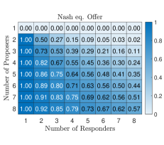
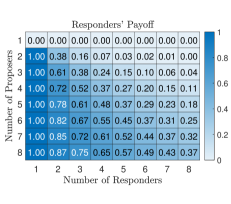
Figure 2: Numeric values of the proposers’ Nash equilibria offers from (13) (left) and the expected payoffs for the proposers (middle) and the responders (right) under these equilibria (see (14)). These are shown for varying number of responders and proposers, under the assumption that responders play their evolutionarily stable strategy and thus select each proposer with the same probability when the offers are identical.

Next, we focus on offer regimes where the highest offer is bigger than zero, i.e. where $s_{K}>0$. Offer regimes where some of the proposers end up with zero selection probabilities under responders’ evolutionarily stable strategy cannot constitute a subgame-perfect Nash equilibrium. The rationale behind this is straightforward: a proposer with a zero probability of being selected will earn no reward, and by simply offering a sufficiently higher amount, any proposer can secure a positive payoff. If we had for any $i:$ $\frac{\partial\Pi_{R}}{\partial p_{i}}<0$ (see (9) and (10)), then this would give a zero selection probability for proposer $i$. Thus, we can restrict our search only to those regimes where the system of equations $\frac{\partial\Pi_{R}}{\partial p_{i}}$ from (9) is equal to zero for all $i\in\{1,2,\dots,K-1\}$ and $p_{i}\neq 0$ for all $i\in\{1,2,\dots,K\}.$ Then it is true for all $i\in\{1,2,\dots,K-1\}$ that:

$$C:=\frac{s_{i}}{p_{i}}\left(1-(1-p_{i})^{L}\right)=\frac{s_{K}}{p_{K}}\left(1-(1-p_{K})^{L}\right)\ .$$

Additionally, we know that the payoff of proposer $i$ with offer $s_{i}$ is given as:

$$\Pi_{P,i}=(1-s_{i})\left(1-(1-p_{i})^{L}\right)\ .$$

In order to find the subgame-perfect Nash equilibrium of proposers (for details see Theorem 3 in the Supplementary Information, ”General Case”) we look at the derivative:

$$\frac{\partial\Pi_{P,i}}{\partial s_{i}} =\left(\frac{g_{i}^{2}C}{s_{i}^{3}H}-\frac{g_{i}C}{s_{i}^{2}}\right)\left(L(1-p_{i})^{L-1}-C\right)-\frac{p_{i}g_{i}C}{s_{i}^{2}H}\ ,$$ (12)

where $g_{i}=\frac{p_{i}^{2}}{(1-p_{i})^{L-1}(Lp_{i}+1-p_{i})-1}$ and $H=\sum_{j=1}^{K}\frac{g_{j}}{s_{j}}$. In the equilibrium, the derivative in (12) has to be equal to zero for all $i\in\{1,2,\dots,K\}.$ In Theorem 3 (see the Supplementary Information) we show that such solutions must be symmetric, i.e. $s_{i}=s,s\in(0,1)$ for all $i\in\{1,2,\dots,K\}.$ In that case also the selection probabilities of responders are symmetric $p_{i}=p=\frac{1}{K}$ for all $i\in\{1,2,\dots,K\},$ since this solution satisfies the conditions for the unique responders’ ESS strategy. Taking all this into account, solving the system in (12) being equal to zero is equivalent to solving:

$$0 =\left(\frac{g}{s}-H\right)\left(L(1-p)^{L-1}-C\right)-p\ ,$$

where $g=\frac{p^{2}}{(1-p)^{L-1}(Lp+1-p)-1}$, $H=K\frac{g}{s}$ and $C=\frac{s}{p}\left(1-(1-p)^{L}\right)$. From this we can derive the unique solution $s^{*}:$

$$s^{*} =\frac{g(1-K)L(1-p)^{L-1}}{g(1-K)\frac{1-(1-p)^{L}}{p}+p}\ .$$

By submitting $p=\frac{1}{K}$ we get:

$$s^{*} =\frac{L(K-1)^{L}}{K^{L+1}-(K-1)^{L-1}((K-1)K+L)}.$$ (13)

It is easy to show that $s^{*}\in(0,1)$ for all $K,L\geq 2$ and that the second derivative of (12) is always negative (see Proposition 1 in the Supplementary Information). Therefore, $s^{*}$ in (13) is indeed a subgame-perfect Nash equilibrium under the assumption that responders behave according to the evolutionarily stable strategy. Apart from the degenerate case of all offers being equal to zero, this is the only subgame-perfect Nash equilibrium. The expected payoff of proposers and responders is:

$$\Pi_{P} =(1-s^{*})\left(1-\left(1-\frac{1}{K}\right)^{L}\right),$$ (14)

$$\Pi_{R} =s^{*}\frac{K}{L}\left(1-\left(1-\frac{1}{K}\right)^{L}\right).$$

Next, we analyse the result in (13) and investigate how the competition (im)balance of both sides of the market influences the thresholds $s^{*}$. Numeric values of equilibrium offers and equilibrium payoffs for a small number of proposers and responders are shown in Fig. 2. One can notice, that for a fixed number of proposers ($\geq 2$) and an increasing number of responders, i.e. increasing responder competition, the equilibrium offers decrease. On the other hand, for a fixed number of responders ($\geq 2$) and increasing proposer competition, the proposers’ offers increase. This observation aligns with intuitive expectations about the effect of competition. The expected payoffs for responders and proposers follow the same trend. The proposers achieve the highest expected payoff when a single proposer faces any number of responders. Conversely, a responder gains the most when they are the sole responder facing at least two proposers. Subsequently, we shall examine the Nash equilibrium strategy and payoffs of both proposers and responders in the asymptotic scenario where $K\gg 1$ and $L\gg 1$ and the ratio of the number of proposers to the number of responders is determined by a constant factor $c>0,$ i.e. $K=cL.$ A low value of $c$ means there is strong responder competition, high $c$ implies strong proposer competition. Then the equilibrium $s^{*}$ depends on $c$ as:

$$s^{*}_{c}=\frac{1}{c(e^{\frac{1}{c}}-1)}\ .$$ (15)

The payoff of the proposers and responders in this asymptotic situation is:

$$\lim_{L\to\infty}\Pi_{P} =1-\frac{c+1}{e^{\frac{1}{c}}c}\ ,\quad\lim_{L\to\infty}\Pi_{R} =\frac{1}{e^{\frac{1}{c}}}\ .$$ (16)

In Fig. 3 we plot the results from  (15) and (16). One can see how variations in the competition factor $c$ impact the offers and payoffs in the limit.

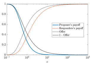
Figure 3: The expected payoff for proposers (blue), for responders (red dotted), the offer level (black) and 1-the offer level (black dotted) in subgame-perfect Nash equilibrium with respect to the proposer-responder ratio $c$, i.e. $K=cL$, in the large $L$ limit (compare (15) and (16)). The differences between the offer and expected payoffs arise from ”inefficiencies”. That is, with some probability some responders choose the same proposer and some proposers may not get chosen by any responder.

In the next section, we look deeper into our analysis and explore possible implications of the MPMR UG on fairness.

Discussion

Throughout our evolutionary history, the interactions within social communities have played a crucial role in shaping the behaviour of our species. Many of these interactions were not interactions in pairs but rather in groups, suggesting that the MPMR UG with multiple players on both sides can contribute to the ongoing debate on fairness extending beyond the insights provided by the one vs. one UG. In this section, we will discuss some of these potential implications.

The perception of what is a fair or equitable division might be impacted by the properties of the community one is part of. For example, individuals with a particular skill or opportunity might represent the proposers, while unskilled individuals, who are still essential for task completion, are the responders. Our model suggests that if responders perceive a shortage of skilled individuals, they may place greater value on this expertise and, consequently, find it fair to accept a smaller share of the reward in exchange for assisting the proposer.

Then a central question arises: what is the underlying sense of group size balance between proposers and responders (i.e. proposer-responder ratio $c$) in the (local) community? And consequently, what would responders deem a fair share of the reward in such a situation? A basic initial assumption could be a balanced scenario where the number of proposers equals that of responders, i.e. when $c=1$. In this case, the subgame-perfect Nash equilibrium offer $s^{*}_{1}$ is equal to $\approx 0.582,$ which is slightly above the equality threshold of $0.5.$ The expected payoff of responders is $\approx 0.368$ and of proposers is $\approx 0.264$ (see (15) and (16)). When a responder is directly approached by a proposer (resembling the one vs. one UG), they may deem it fair to receive a share of the reward equivalent to what they would obtain in the community setting of the MPMR UG, i.e. 36.87% of the reward.

However, when $c=1$, a proposer receives a smaller payoff than a responder. Drawing from the previous analogy, we might anticipate a decrease in the number of individuals specializing in the skill until the payoff difference is eliminated. Such an ”equity” ratio $c$ when the payoffs for members of both groups are identical is $c=0.872,$ meaning there are fewer proposers than responders. The payoff of each proposer and responder is approximately $0.318$ and the proposers’ offers are around $0.534.$ Once again, a responder could deem it fair to get the same payoff of $0.318$ from the one vs. one interaction with a proposer as they would enjoy in the MPMR UG scenario with many players.

Note if there is some cost the proposer has to pay in order to be able to split and share the reward (e.g. energy and time invested for training to acquire a skill, or alternatively, to find an opportunity) their actual payoff is lower accordingly. This moves the blue curve of the proposers’ payoff in Fig. 3 down, changing the equity ratio to a lower number, leading to an even smaller proportion of proposers in the community and finally smaller rewards for the responders in the equity state.

Next, let us compare the derived thresholds with the literature on the UG and the Dictator Game in which the responder cannot refuse the split and gets what is offered by the proposer.

As an indication of fairness norms, one might look at the outcomes of the Dictator Game. Even though their offers cannot be refused, proposers in experiments often give a positive reward to the responder. In a meta-analysis by Engel [36] the mean offer in the Dictator Game was $28\%$ with a modal (i.e. typical) offer of zero among W.E.I.R.D. societies. Conversely, in three small-scale societies, Henrich et al. [4] found mean offers of 20%, 31%, and 32% percent and only a few subjects offered zero. Another recent meta-analysis by Cochard et al. [37] supports the results with a calculated mean offer of 30.6% in the Dictator Game. We can notice these values are very close to our estimated payoff of the responder in the balanced case (31.8%).

In a meta-analysis of UG studies, Oosterbeek et al. [5] found a mean offer of $40\%$ and Cochard et al. [37] found the mean to be $42.58\%.$ Henrich et al. [4] conducted experiments within small-scale societies and found the mean offers ranging from 26 % to 58% for different societies. One can ask whether proposers’ behaviour can be attributed to fairness concerns or simply strategic behaviour, wherein they offer proposals that maximise their payoffs given the assumed distribution of acceptance among responders. For example, Roth et al. [29] found evidence supporting strategic behaviour among proposers. On the other hand, Henrich et al. [4] concluded that offers tend to be higher than the optimal payoff-maximizing offer, presumably due to pessimism regarding rejection frequencies and ambiguity aversion. These payoff maximizing offers are found to be around 25%-40% for different small-scale societies. Nevertheless, Henrich et al. also noted instances where certain groups exhibited a tendency to accept nearly all low offers, while other groups commonly rejected high offers. Furthermore, Solnick [38] found the average minimally acceptable offer (the offer below which the responder rejects the offer) to be 30.8%. Once again, the thresholds are quite similar to the ones proposed from the MPMR UG.

Other authors, e.g. Schuster [39], claim the Golden Ratio, of about 0.618 vs. about 0.382, to be the solution for fair thresholds and supports this claim by providing numerous examples from the literature that illustrate real-life situations exhibiting similar patterns. This threshold is once again close to ours, even though the author describes different mechanisms for achieving it.

Conclusions

We have proposed a multi-player version of the UG, which we named the Multi-Proposer-Multi-Responder Ultimatum Game, with multiple responders and proposers playing simultaneously. Our work offers a new perspective on the UG with the interplay between proposer and responder competition. We analysed the responders’ strategy patterns and found that there can be a continuum of Nash equilibria of responders for some subgames (determined by offers from proposers), however, there is only one unique evolutionarily stable strategy in each subgame. We analytically derive subgame-perfect Nash equilibria of the proposers with respect to this strategy, and find that situations with multiple proposers and responders in both groups lead to non-trivial offer values. These are unique for each parameter regime (except for the degenerate solutions of all offers being zero). We stress that our model does not include bargaining sequential dynamics to reach non-trivial offer levels and we achieve this under a one-shot setting. Admittedly, the game’s assumptions are heavily simplified when compared to complex economic and societal realities. We consider all goods (or jobs, flowers, goods etc.) to be of identical quality, all with the possibility to be reached in the same way and we assume all responders have full information of all the proposals. Yet, we believe there is an untapped potential in examining notions of fairness within the context of larger groups of players. Since real-world interactions rarely involve just two individuals, and the presence of external alternatives remains pertinent, we believe this expanded viewpoint can shed more light on our understanding of why fairness is perceived as it is.

Our analysis has revealed the potential impact of the ratio between the (asymptotic) number of proposers and responders on the perception of fairness in multi-player scenarios. We postulate that the sense of fairness within these scenarios then subconsciously influences people’s behaviour in the UG laboratory experiments. In particular for the UG played on social networks, MPMR UG-like situations happen naturally in the neighbourhood of individuals. Conversely, the MPMR UG can explain the incentives for the way social networks evolve and restructure. We compared these insights with the experimental literature of one vs. one UG and Dictator Game and found them to be of intriguing similarity.

We stress we do not claim the MPMR UG to be the sole explanation of the observed behaviour, rather, we suggest it as a noteworthy addition to the ongoing discussion on fairness.