Online Fair Allocation with Best-of-Many-Worlds Guarantees

Abstract

We investigate the online fair allocation problem with sequentially arriving items under various input models, with the goal of balancing fairness and efficiency. We propose the unconstrained PACE (Pacing According to Current Estimated utility) algorithm, a parameter-free allocation dynamic that requires no prior knowledge of the input while using only integral allocations. PACE attains near-optimal convergence or approximation guarantees under stationary, stochastic-but-nonstationary, and adversarial input types, thereby achieving the first best-of-many-worlds guarantee in online fair allocation. Beyond theoretical bounds, PACE is highly simple, efficient, and decentralized, and is thus likely to perform well on a broad range of real-world inputs. Numerical results support the conclusion that PACE works well under a variety of input models. We find that PACE performs very well on two real-world datasets even under the true temporal arrivals in the data, which are highly nonstationary.

1 Introduction

We study the problem of online fair allocation, where items arrive sequentially in $t$ time steps, and we need to distribute them among a set of $n$ agents with heterogeneous preferences, aiming to balance fairness and efficiency. At each time step, we observe the unit value of each agent for an item, and make an irrevocable allocation. The agents are assumed to have linear and additive utilities. This setting captures scenarios including allocating food to food banks Gorokh et al. (2021); Sinclair et al. (2022), fair recommender systems (Murray et al., 2020), Internet advertising (Conitzer et al., 2022a), file-sharing protocols (Wu and Zhang, 2007), and many more. These real-world systems often feature large horizon length, and high volume and frequency of item arrivals.

Fair allocation in our setting is closely related to the concept of Fisher market equilibrium. In the offline fair allocation setting, solving the classical Eisenberg-Gale (EG) convex program (Eisenberg and Gale, 1959) gives a competitive equilibrium from equal incomes (CEEI), which gives strong properties in terms of both fairness and efficiency, e.g. envy-freeness, proportionality, and Pareto-optimality. For stochastic items with continuous supply, an infinite-dimensional analogue is given by Gao and Kroer (2023). A natural goal for our online setting is then to design an algorithm that converges to the hindsight CEEI solution, or attains good performance relative to it, in an online manner.

In real-world allocation problems, it may be hard to ensure that the input (items, in our case) adheres to a particular class of assumptions. For example, assuming that the items are sampled from a fixed distribution at each time step may allow for the best convergence guarantees, but this assumption may not be suitable in all settings. Conversely, one may resort to adversarial guarantees that optimize performance against worst-case input. Yet such worst-case guarantees can be very conservative, and may indeed be too conservative for settings where the items are generated from a more benign process. Existing online fair allocation algorithms are all designed specifically for either stochastic or worst-case input, and fail to achieve desirable guarantees when the input is not derived according to the assumed model. For stochastic inputs, Gao et al. (2021) showed an algorithm that converges to the optimal Fisher market solution asymptotically, but even moderately adversarial input may lead to highly unfair allocations. For adversarial inputs, Azar et al. (2016); Banerjee et al. (2022); Huang et al. (2022) develop approximation algorithms with competitive ratio guarantees, but they are far from desirable in the stochastic case, as they make highly conservative decisions in order to give guarantees in the adversarial setting.

To this end, we focus on developing a simple and robust online fair allocation algorithm that achieves strong asymptotic performance, while being oblivious to the input model, i.e., without any information about the type of input that will be generated. The algorithm we develop achieves a best of many worlds guarantee: It achieves strong convergence bounds with stationary, nonstationary-yet-stochastic data, and also attains good performance with adversarial data, all relative to the hindsight optimal allocation.

1.1 Our Contributions

We propose the unconstrained PACE (Pacing According to Current Estimated utility) algorithm (see Algorithm 1), which is the first algorithm to simultaneously attain performance guarantees under stationary, nonstationary, and adversarial input.

The unconstrained PACE algorithm is an adaptation of the earlier constrained PACE algorithm (Gao et al., 2021), where we remove the requirement of projection in each step of the algorithm. This is a nontrivial improvement, as it enables the interpretation into a primal greedy algorithm, and leads to adversarial guarantees, which are impossible for the previous algorithm. Moreover, as opposed to the previous algorithm, unconstrained PACE becomes free of any prior knowledge about the input values. In this paper, we will refer to our unconstrained algorithm as “PACE”, and the previous algorithm by Gao et al. (2021) as “constrained PACE” explicitly.

Our algorithm has useful interpretations in both the primal and dual spaces of the EG convex program. In the dual space, PACE is equivalent to an unconstrained variant of dual averaging (Nesterov, 2009; Xiao, 2009), a stochastic optimization algorithm; this equivalence arises because the agent utility vector is a subgradient for the dual Eisenberg-Gale problem (Section 4.1). Gao et al. (2021) previously leveraged this connection to DA for the constrained case, but all their arguments crucially relied on being able to bound the iterates of the algorithm via projection. In the primal space, PACE can be interpreted as a first-order, integral greedy algorithm, which myopically optimizes the approximated increment to the EG objective (Section 4.2); the primal perspective is important for our adversarial analysis.

We study PACE’s performance guarantees in the asymptotic sense of horizon length $t$, while we also show the dependence on $n$ and other parameters that characterize the input. PACE is tuning free, and obtains good performance under different input models without knowing what type of data it is facing:

• Stationary data (Section 5). When agent values at each step is independently and identically (i.i.d.) drawn from an unknown distribution, PACE results in agent time-averaged utilities that converge to the hindsight optimum at a $O(\log t/t)$ rate. Similar convergence guarantees hold for envy, and if budgets are taken into account, spending and regret.

• Nonstationary data (Section 6). We consider several non-stationary stochastic input models: ergodic data and block-wise independent data with corruptions. We show that the guarantees for the i.i.d. case are still preserved under such inputs, up to additive error that measures the degree of nonstationarity. The dependency on the nonstationary parameters is smooth, which shows the robustness of PACE and fills the gap between stationary and adversarial inputs.

• Adversarial data (Section 6). For adversarially chosen data, we show that PACE achieve multiplicative envy and competitive ratio bounds with logarithmic dependence on a parameter $\varepsilon$, which characterizes the extremity of input (Section 7.1). When $\varepsilon$ is constant, the bounds are free of horizon length $t$, i.e. PACE guarantees a fixed fraction of the hindsight allocation. We also develop $O(\log t)$ competitive ratio bounds from an alternative perspective, seed utility, which admits a initial utility $\gamma$ to each agent (Section 7.2).

The best-of-many-worlds guarantees show that PACE performs well under a broad range of inputs. Since it is completely free of tuning parameters and prior knowledge, we believe PACE is a natural and robust dynamic for the online fair allocation problem in a general sense. Besides, PACE is highly simple and decentralized, making it desirable for large-scale real-world applications.

Relationship to our earlier conference papers on PACE.

Let us briefly comment on how this paper supersedes and extends our prior work on online fair allocation.

• For online fair allocation under nonstationary input models, the present paper supersedes Liao et al. (2022), which is based on the constrained version of PACE from Gao et al. (2021). However, Liao et al. (2022) also provides more general convergence analysis results for the dual-averaging algorithm in online convex optimization (OCO) under nonstationarity. Our paper focuses exclusively on online fair allocation, and thus does not supersede those more general results. It is an interesting question how to generalize our unconstrained convergence results for PACE to more general OCO problems.

• For online fair allocation with adversarial inputs, the present paper supersedes Yang et al. (2024), which develops guarantees for both constrained and unconstrained PACE. The guarantees for unconstrained PACE in Yang et al. (2024) were stronger than those for constrained PACE (by requiring much milder assumptions to achieve the same bounds). The main point in developing the weaker guarantees for constrained PACE was that constrained PACE was, at the time, the only variant known to have guarantees under stochastic and nonstationary input. Since we will be developing stochastic-input guarantees for unconstrained PACE in this paper that are asymptotically as good as the ones for constrained PACE in Gao et al. (2021); Liao et al. (2022), we conclude that unconstrained PACE is the more natural and robust algorithm, and thus omit the adversarial results for constrained PACE in Yang et al. (2024).

2 Related Work

2.0.1 Convex optimization for market equilibria.

Convex optimization algorithms and their theory have been applied to computing competitive market equilibria, which has been of interest in economics and computation for a long time (Nisan et al., 2007). The computation of static Fisher market equilibrium with divisible items is captured by the Eisenberg-Gale convex program (Eisenberg and Gale, 1959), which also has an infinite-dimensional generalization with stochastic items (Gao and Kroer, 2023). Specific cases of finite-dimensional static Fisher markets are studied through various convex optimization formulations (Birnbaum et al., 2011; Kroer et al., 2019; Shmyrev, 2009; Gao and Kroer, 2020). Applying first-order methods to equilibrium-capturing convex programs often leads to interpretable market dynamics that emulate real-world market-behaviors, such as the proportional response (PR) dynamic (Birnbaum et al., 2011; Gao and Kroer, 2020; Zhang, 2011; Cheung et al., 2018a), and tâtonnement (Cheung et al., 2020). The constrained (Gao et al., 2021) and unconstrained PACE algorithms are no exception: they can be interpreted as applying a first-order method (dual averaging) to the dual of Eisenberg-Gale convex program, but can also be interpreted as a natural bidding dynamic in a sequence of first-price auctions.

The Eisenberg-Gale program is equivalent to maximizing Nash welfare (NW) (Nash Jr, 1950) subject to supply feasibility constraints, which is known as a strong proxy for balancing fairness and efficiency (Kaneko and Nakamura, 1979). In the offline setting, there is a line of literature on approximating NW with indivisible items. The problem is APX-hard  Lee (2017), though constant competitive-ratio algorithms are known  Cole and Gkatzelis (2018); Anari et al. (2017); Barman et al. (2018). Beyond additive utilities, there are also competitive-ratio-type results for budget-additive utilities (Garg et al., 2018), separable, piecewise-linear and concave utilities (Anari et al., 2018), and submodular utilities (Garg et al., 2020; Li and Vondrák, 2022; Barman et al., 2020; Chaudhury et al., 2021). Discrete variants of EG (i.e. NW maximization) have been applied to real-world fair division on the spliddit website (Caragiannis et al., 2019). In the discrete case, NW maximization still yields attractive efficiency and fairness guarantees, though the connection to CEEI no longer holds.

2.0.2 Online fair allocation.

We first discuss existing works on online fair allocation with sequentially arriving items, whose objective is to obtain a market-equilibrium type allocation, or based on the optimization EG program or NW. We will also give a sketch for other approaches to the notion of online fair division.

For the online setting with i.i.d. arriving items, Gao et al. (2021) develop the constrained PACE algorithm, and showed that it asymptotically attains online Fisher market equilibrium (Gao and Kroer, 2023) with a $O(\log t/t)$ convergence rate, and similar bounds hold for agent regret and envy. However, to maintain the equivalence of their PACE algorithm and dual averaging (Xiao, 2009), they assume normalization of agent budgets and values, and enforce projection to a fixed domain based on these normalizations. We show that such projection is unnecessary for stochastic inputs, and moreover that the projection is easily corrupted under adversarial inputs. To this end, our unconstrained PACE algorithm is a significant generalization of their constrained version to nonstationary and adversarial input types, while achieving the same asymptotic guarantees under stochastic input without requiring prior knowledge. See a detailed comparison in Section 4.

For the online setting with adversarially arriving items with arbitrary valuations, counterexamples are known which show that no online algorithm can achieve meaningful Nash welfare guarantees (Banerjee et al., 2022). This motivates the investigation of restrictions on the adversarial input that enable nontrivial guarantees. Azar et al. (2016) adopt an assumption that is similar to the first part of our adversarial analysis: the minimum nonzero valuation of each agent is at least an $\varepsilon$ fraction of the agent’s maximum value. They develop guarantees on the utility ratios, which is comparable to NW. However, their $O(\log(nt/\varepsilon))$ upper bound fails to remove the dependence on horizon length $t$, meaning the ratio is unbounded as the sequence length increases. Banerjee et al. (2022) assume access to a prediction of each agent’s total sum of utilities, and provide an algorithm called set-aside greedy (SAG) which has $O(\log n)$ and $O(\log t)$ competitive ratio. However, SAG involves a very conservative design: half of each item is allocated uniformly to each agent, which is far from optimal for non-adversarial input. In Section 7.2, we introduce the idea of seed utility as a more general perspective that can recover a “set-aside” type algorithm similar to theirs. Huang et al. (2022) assumes the input to be $\lambda$-balanced or $\mu$-impartial, where $\lambda$ and $\mu$ characterize the desired properties of the input; their competitive ratio upper bounds are logarithmic in the parameter and $n$. However, their bound still implicitly depends on horizon length $t$; their parameters are not scale invariant, and are NP-hard to compute in advance. We remark that none of above algorithms have good performance guarantees for stochastic inputs, due to their conservative and complex design. Our unconstrained PACE algorithm has a greedy-style interpretation which is similar to the above works, but has convergence guarantees under stochastic input, while still attaining a worst-case competitive ratio that is independent of $t$.

Besides CEEI-style allocations and NW maximization, there is also a line of work which focuses on achieving (possibly approximate) envy-freeness guarantees in the online setting directly. Bogomolnaia et al. (2022) assume stochastic input and enforce envy-freeness as a soft constraint, while maximizing social welfare. He et al. (2019) allow reallocating previous items, and show that $O(T)$ reallocation is enough to achieve envy-freeness up to an item. Benade et al. (2018) considers envy minimization in the stochastic, indivisible setting, and show that allocating each item to each agent uniformly at random is near-optimal. Zeng and Psomas (2020) considers the indivisible setting with a non-adaptive adversary, showing that nontrivial approximation of envy-freeness and Pareto-optimality is hard to achieve simultaneously. While we also give approximate envy-freeness results, we remark that the focus on strict envy-freeness seems to remove the connection to market equilibrium in this line of work. By focusing on CEEI-style allocation rather than directly constraining envy, we get asymptotic envy guarantees, but also achieve other fairness guarantees such as approximate NW maximization, and get stronger efficiency guarantees.

Finally, we briefly comment on lines of work that consider online fair allocation under models that are more significantly different from ours, either in utilities or in the input setup. Liu et al. (2015) studies online allocation for Leontief utilities where each agent wants a bundle with items of fixed proportions, and shows how to balance various properties for this setting. Aleksandrov et al. (2015) studies a simple mechanism where agents can declare if they like an item, and then a coin is flipped to determine which of the agents that desired the item will get it. Bateni et al. (2022) models item arrival with Gaussian valuations and proposes a stochastic approximation scheme based on frequently resolving the EG convex program, which ensures a constant approximation ratio in terms of a proportional fairness metric. Cheung et al. (2018b) considers an evolving market environment and shows that the PR dynamics generates iterates that are close to the changing equilibrium. As in PR dynamics, they assume prior knowledge of future value distributions, while our algorithm does not rely on such input. Gkatzelis et al. (2021) assumes that the valuations are normalized a priori, and studies the setting where items arrive online and with two agents. They focus on satisfying the no-envy condition while maximizing social welfare, and show that one can do this approximately by allocating items proportionally to valuations. Manshadi et al. (2021) studies the problem of rationing a social good and propose simple, implementable algorithms that promote fairness and efficiency. In their setting, it is the agents’ demands rather than the supply that are sequentially realized and possibly correlated over time. Finally, there is also a recent line of online fair allocation literature that considers sequentially arriving agents, instead of items (Jalota and Ye, 2022; Sinclair et al., 2022).

2.0.3 Pacing in online auctions and resource allocation.

The idea of pacing has been studied in the context of budget management for Internet advertising auctions and resource allocation, which can lead to strong revenue and individual optimalityguarantees (Conitzer et al., 2022a, b; Balseiro and Gur, 2019); it is also used widely in practice, as reported by (Conitzer et al., 2022b). The name PACE for our algorithm is meant to invoke this connection. As shown by Balseiro et al. (2023), pacing strategies for budget management can ensure individual best-of-many-world guarantees in terms of optimal budget expenditure over time, under a variety of input models similar to ours. Let us briefly discuss how our work differs from existing best-of-many-worlds type guarantees in online resource allocation (budget management in repeated truthful auctions is a special case of this). In online resource allocation, a sequence of requests arrive over time, with each request consisting of a reward and cost function, and at each time step the algorithm must select a decision to maximize the sum of rewards while satisfying long-term cost constraints on each resource. In that setting, strong best-of-many-worlds guarantees are known (Balseiro et al., 2023; Celli et al., 2022; Castiglioni et al., 2022). The objective in the online resource allocation setting has time separability, i.e., is of the form $\sum_{t=1}^{T}f_{t}(x)$. Time separability is crucial for the regret bounds in these works, as it enables translating dual regret to primal regret through weak duality. However, in our setting time-separability no longer holds, since our objective is the sum of the logarithms of agent utilities. Therefore, our results cannot be derived with similar techniques to those papers. Moreover, the types of competitive-ratio guarantees achieved e.g. by Balseiro et al. (2023) are impossible in the online fair allocation setting, where hard input sequences that preclude such strong and general guarantees are known (Banerjee et al., 2022; Gao et al., 2021).

2.0.4 Online convex optimization

Next, we discuss briefly how our problem differs from existing literature in online convex optimization. For stochastic input, our algorithm can be interpreted as stochastic dual averaging (Xiao, 2009) without an external regularizer. However, because our problem has an open domain and an objective which is neither bounded nor strongly convex, the results from (Xiao, 2009) cannot be applied to our problem. In Theorem 5.1 we redevelop the convergence theory of dual averaging with implicit bounds, which is a technically novel approach to handle unbounded domains; our nonstationary results also generalize the input models of (Xiao, 2009), which only considered i.i.d. stochastic data. The framework of online stochastic convex programming by (Agrawal and Devanur, 2014) cannot be applied to our fair allocation setting either. They assume a bounded domain known in advance and Lipschitz gradients; both conditions fail for both our primal and dual problems. Secondly, they only have performance guarantees for the objective, while we are able to give convergence results for the average utility of each individual agent. Hence their results are not applicable to our stationary case, let alone the nonstationary and adversarial cases, which are not considered in that work.

3 Preliminaries

An online fair allocation instance consists of a 4-tuple $\mathsf{S}=(t,n,B,\gamma)$, where

• $t$ is the length of the finite horizon (our algorithm does not need to know $t$).

• $n$ is the number of agents. The set of agent is $[n]$.

• $B=(B_{1},\cdots,B_{n})\in\mathbb{R}_{++}^{n}$ is the weight, or priority, of agents. In the Fisher market interpretation of our setting, these are the budgets.

• $\gamma=(v^{1},\cdots,v^{t})$ is the input value sequence. For each $\tau\in[t]$, $v^{\tau}\in V$ where $V\subset\mathbb{R}_{+}^{n}$ is the set of possible value vectors. For agent $i$, their valuation sequence is denoted by $v_{i}=(v_{i}^{1},\cdots,v_{i}^{t})\in\mathbb{R}_{+}^{t}$, where $v_{i}^{\tau}$ denotes their unit value for the item at time step $\tau$. We also refer to $\gamma=(v_{i}^{\tau})^{n\times t}$ as the input matrix, whose columns are revealed sequentially.

Given an input instance, the decision maker allocates the stream of items one at a time in an irrevocable manner, without seeing the future items. At time step $\tau$, a unit-supply item is revealed, and the decision maker must choose an allocation $x^{\tau}=(x_{1}^{\tau},\cdots,x_{n}^{\tau})\in\Delta_{n}$ ($\Delta_{n}$ is the simplex in $\mathbb{R}^{n}$), based on information available at that time, and distribute the item accordingly. Here the $i$-th entry of $x^{\tau}$ is the fraction of item $\tau$ allocated to agent $i$ (we emphasize that our eventual PACE algorithm does not need to perform fractional alloccation). On receiving her fraction, agent $i$ realizes an instantaneous utility of $u_{i}^{\tau}:=v_{i}^{\tau}x_{i}^{\tau}$. The agent utilities are linear and additive. We let $x_{i}=(x^{1}_{i},\cdots,x^{t}_{i})$ denote the allocation agent $i$ receive over time. Let $U_{i}^{\tau}=\sum_{t^{\prime}=1}^{\tau}u_{i}^{t^{\prime}}$ be the total utility of agent $i$ up to time step $\tau$, and $\bar{u}_{i}^{\tau}=U_{i}^{\tau}/\tau$ be the time-averaged utility at time step $\tau$. The goal of the decision maker is to choose, in an online manner, an allocation $x$ such that it achieves some form of efficiency and fairness guarantees.

We consider three different types of input models: 1) stationary, or i.i.d. input, 2) nonstationary-yet-stochastic input, and 3) adversarial input. For the first two stochastic input types, we let $\Omega$ be the sample space of $\gamma$, $Q^{\tau}\in\Delta(V)$ be the marginal distribution of the $\tau$-step agent values $v^{\tau}:=(v_{1}^{\tau},\cdots,v_{n}^{\tau})$, and $\bar{Q}=(1/t)\sum_{\tau=1}^{t}Q^{\tau}$. We assume $t\geq n$, so each agent gets at least one item under integral allocation. We also assume that agent values are bounded, i.e., $\|v\|_{\infty}:=\max_{i}\|v_{i}\|_{\infty}<\infty$. However, we stress that the PACE dynamic that we study generalizes to infinite values, and is not going to require access to $V,Q^{\tau},\|v\|_{\infty}$, or any other parameter of the input value distribution. It is a prior-free, tuning-free algorithm that, at any given time $\tau$, requires knowing only $n,B$, and the inputs from time 1 to $\tau$; the parameters characterizing the input in this paper are only required in the analysis of theoretical bounds. We also emphasize that PACE does not need to know the time horizon $t$; this is again only required when discussing our theoretical bounds.

3.1 Benchmark: The Hindsight Allocation

As a benchmark, we will consider the hindsight-optimal allocation. Suppose all the items are presented to the decision maker offline, as opposed to arriving one by one. In that case, a fair and efficient allocation can be found by allocating using the Eisenberg-Gale (EG) convex program (Eisenberg and Gale, 1959). EG gives the allocation that maximizes the sum of weighted logarithmic utilities (which is equivalent to maximizing the weighted geometric mean of utilities):

$$\max_{x\geq 0,U\geq 0}\left\{\left.\sum_{i=1}^{n}B_{i}\log U_{i}\ \right|U_{i}\leq\langle v_{i},x_{i}\rangle\ \forall i\in[n],\ \sum_{i=1}^{n}x_{i}^{\tau}\leq 1\ \forall\tau\in[t]\right\}.$$ (1)

We remark that the weights $B_{i}$ can be interpreted as budgets in a market-based interpretation of the Eisenberg-Gale allocation; the allocation and dual variables on the supply constraints form a competitive equilibrium in the corresponding Fisher market; see Section 0.A.1 for more details on this interpretation. If all budgets are equal then EG yields a CEEI allocation.

The dual program of (1) is

$$\min_{\beta\geq 0}\left\{\frac{1}{t}\sum_{\tau=1}^{t}\max_{i\in[n]}\beta_{i}v_{i}^{\tau}-\sum_{i=1}^{n}B_{i}\log\beta_{i}\right\}.$$ (2)

For a value sequence $\gamma$, we let $x^{\gamma}$ denote the optimal hindsight allocation, which is an optimal solution to (1), and we denote the resulting utilities as

$$U_{i}^{\gamma}=\langle v_{i},x_{i}^{\gamma}\rangle=\sum_{\tau=1}^{t}x_{i}^{\gamma,\tau}v_{i}^{\tau},\ \ u_{i}^{\gamma}:=(1/t)\cdot U_{i}^{\gamma}.$$

For stochastic inputs, we will also be interested in the underlying problem where item supplies are given by their average probability of being sampled, i.e. $s=\mathrm{d}\bar{Q}/\mathrm{d}\nu$. Letting $\langle v_{i},x_{i}\rangle:=\int_{V}v_{i}x_{i}\mathrm{d}\nu$, this leads to the infinite-dimensional analogue of (1).

$$\max_{x\in L^{\infty}_{+}(V),u\geq 0}\left\{\left.\sum_{i=1}^{n}B_{i}\log u_{i}\ \right|\ u_{i}\leq\langle v_{i},x_{i}\rangle\ \forall i\in[n],\ \sum_{i=1}^{n}x_{i}\leq s\right\}.$$ (3)

We let $x^{*},u^{*}$ denote the optimal solutions in (3). The infinite-dimensional analogue of (2) is the following.

$$\min_{\beta\geq 0}\left\{\int_{V}\left(\max_{i\in[n]}\beta_{i}v_{i}\right)\mathrm{d}\bar{Q}-\sum_{i=1}^{n}B_{i}\log\beta_{i}\right\}.$$ (4)

A rigorous mathematical treatment of the infinite-dimensional program can be found in Gao and Kroer (2023) and Gao et al. (2021), Section 2. Let $\beta^{*}$ be the optimal solution of (4). Notice that

$$\beta^{*}=\arg\min_{\beta\geq 0}\phi(\beta),\ \phi(\beta):=\mathbb{E}_{v\sim\bar{Q}}\left[\max_{i\in[n]}\beta_{i}v_{i}-\sum_{i=1}^{n}B_{i}\log\beta_{i}\right].$$ (5)

This allows (4) to be interpreted as a stochastic online learning problem.

It is well-known that the hindsight allocation generated by the EG program enjoys the following strong efficiency and fairness properties. The same properties hold for $x^{*}$ in the underlying market.

1. Pareto optimality: we cannot strictly increase any agent’s utility without decreasing some other agents’ utility.

2. Envy-freeness: each agent prefers their own allocation to that of any other agent, in a budget-adjusted sense: $\langle v_{i},x_{i}^{\gamma}\rangle/B_{i}\geq\langle v_{i},x_{j}^{\gamma}\rangle/B_{j}$ for all $j\neq i$.

3. Proportionality: every agent achieves at least as much utility as under the uniform allocation, i.e. $\langle v_{i},x_{i}^{\gamma}\rangle\geq B_{i}\cdot\langle v_{i},1_{t}\rangle$ for all $i$.

4. Invariance to agent value scaling: if $x_{i}^{\gamma}$ is a hindsight optimal solution for values $(v_{1},\cdots,v_{n})$, then it is also a hindsight optimal solution for $(\alpha_{1}v_{1},\cdots,\alpha_{n}v_{n})$, where $\alpha_{i}>0$ are arbitrary positive constants.

3.2 Performance Metrics

We now introduce the performance metrics that we will focus on. We will focus on deriving bounds on the performance on these metrics as a function of $t$. The number of agents $n$ is fixed for each problem instance, but we will also explicitly describe how our bounds depend on $n$, which was left open by previous analysis in the stochastic case (Gao et al., 2021).

Metrics for stochastic inputs.

For stationary and nonstationary-yet-stochastic inputs, we consider the mean-square difference between the mean agent utility achieved by our algorithm, $\bar{u}^{t}$, and the optimal time-averaged utilities of the underlying Fisher market $u^{*}$:

$$\mathbb{E}_{\gamma\in Q}\|\bar{u}^{t}-u^{*}\|^{2}.$$

Bounds on this quantity also imply bounds of the same order for convergence to $u^{\gamma}$, the hindsight optimal allocation. With mean-square convergence, we also consider the regret and additive envy of agents. The regret of agent $i$ is the difference between the hindsight equilibrium utility $U_{i}^{\gamma}$ and their realized utilities, averaged over time:

$$\mathrm{Regret}_{i}^{t}(\gamma):=\max\left\{u_{i}^{\gamma}-\bar{u}_{i}^{t},0\right\}.$$

The additive envy of an agent captures how much they prefer another agent’s allocation to their own. Formally, it is defined as

$$\mathrm{Envy}_{i}^{t}(\gamma):=\max_{k}\bar{u}_{ik}^{t}/B_{k}-\bar{u}_{i}^{t}/B_{i},$$

where $\bar{u}_{ik}^{t}=(1/t)\cdot\langle v_{i},x_{k}\rangle$ is buyer $i$’s time-averaged utility if they were to be given agent $k$’s allocation instead of their own.

Metrics for adversarial input.

For adversarial input it is impossible to converge to $u^{\gamma}$ with online inputs (Banerjee et al., 2022; Yang et al., 2024). Instead, we instead study how well the PACE dynamics approximate the objective of the hindsight EG program. In particular, we consider the Nash welfare, i.e. the weighted geometric mean of agent utilities. We measure the competitive ratio (CR) w.r.t. NW:

$$\mathrm{CR}(\gamma):=\prod_{i=1}^{n}\left(\frac{U_{i}^{\gamma}}{U_{i}^{t}}\right)^{B_{i}/\|B\|_{1}}.$$

Notice that Nash welfare is equivalent to (1) in terms of maximization, and invariant to agent value scaling. We believe scale-invariant multiplicative metics are natural for the adversarial setting, since scale invariance is a fundamental property of the hindsight solution as well. Both the hindsight optimal solution to (1) and PACE’s allocation are scale invariant.

In our analysis under adversarial input, we will also develop guarantees on the following utility ratio

$$R({\gamma}):=\sup_{\widetilde{U}}\left\{\sum_{i=1}^{n}\frac{B_{i}}{\|B\|_{1}}\cdot\frac{\widetilde{U}_{i}}{U_{i}}\right\},$$

where the supremum is taken over all feasible hindsight allocations $\widetilde{U}$. By the AM-GM inequality, we know that $R(\gamma)$ is an upper bound on the competitive ratio w.r.t. NW:

$$R({\gamma})\geq\sum_{i=1}^{n}\frac{B_{i}}{\|B\|_{1}}\cdot\frac{{U}^{\gamma}_{i}}{U_{i}}\geq\mathrm{CR}(\gamma).$$

For agent envy in the adversarial case we consider multiplicative envy instead of additive envy, which is again scale invariant:

$$\textnormal{Multiplicative-Envy}_{i}(\gamma):=\max_{k\neq i}\frac{B_{i}}{B_{k}}\cdot\frac{\max_{k}\bar{u}_{ik}^{t}}{\bar{u}_{i}^{t}}.$$

4 The PACE Algorithm

This section presents our proposed algorithm, unconstrained PACE (Pace According to Current Estimated utility), and its interpretations under both stochastic and adversarial input models.

At every time step $\tau$, an item arrives and the agent valuations for the item are revealed. PACE then simulates a first-price auction: Each agent places a bid for the item, which is equal to their value multiplied by the current pacing multiplier $\beta_{i}^{\tau}$. The whole item is allocated to the highest bidder, preferring the bidder with the smallest index for tie-breaking (any other tie-breaking rule will work as well). Each agent then observes their realized utility at this time step, and updates their current estimated utility. The pacing multiplier is updated to be an agent’s weight $B_{i}$ divided by their estimated utility. The algorithmic details are displayed in Algorithm 1.

Input: number of agents $n$, agent weights $B$.

Initialization: $\beta^{1}=1^{n}$.

for $\tau=1,\cdots,$, do

       Observe agent valuation $v^{\tau}$. Simulate an auction where agent $i$ bids $\beta_{i}^{\tau}v_{i}^{\tau}$. The whole item $\tau$ is allocated to the highest bidder, with lexicographical tie-breaking:

$$i^{\tau}:=\min\left\{\arg\max_{i\in[n]}\beta_{i}^{\tau}v_{i}^{\tau}\right\},\ \ x_{i}^{\tau}=\bm{1}(i=i^{\tau}).$$

Agent $i$ updates their estimated utility

$$\bar{u}_{i}^{\tau}=\frac{1}{\tau}\cdot x_{i}^{\tau}v_{i}^{\tau}+\frac{\tau-1}{\tau}\bar{u}_{i}^{\tau-1}.$$

Agent $i$ updates the pacing multiplier

$$\beta_{i}^{\tau+1}=\frac{B_{i}}{\bar{u}_{i}^{\tau}}$$

Algorithm 1 PACE (unconstrained)

Algorithm 1 is based on a constrained version of PACE, initially proposed by Gao et al. (2021). In constrained PACE, at each time step, the pacing multiplier of each agent is projected to a fixed interval $\left[B_{i}/(1+\delta_{0}),B_{i}\cdot(1+\delta_{0})\right]$. While Algorithm 1 simply modifies the constrained algorithm by removing the projection, we are going to show that this small change leads to major improvements:

• For the projection, constrained PACE requires a normalization of agent weights $\sum_{i\in[n]}B_{i}=1$ and item values per agent $\int_{V}v_{i}\mathrm{d}v=1,\forall i\in[n]$, which implicitly involves prior knowledge of agent values. Unconstrained PACE, in contrast, requires no such assumptions to achieve theoretical guarantees.

• In the stochastic case, constrained PACE enforces the projection to achieve strict equivalence to dual averaging, with bounded domain and strong convexity. However, by improving the analysis technically, unconstrained PACE can be shown to have a convergence rate of the same order.

• In the adversarial case, constrained PACE is easily corrupted by bad input instances, see the example in Section 0.A.4 Conversely, unconstrained PACE has a natural interpretation as a greedy-style algorithm, and achieves worst-case guarantees.

We also remark that the PACE algorithm has a series of desirable properties for real-world applications:
Highlight 1. PACE is simple and decentralized. The PACE dynamics can be run in either centralized (by having the mechanism designer emulate the pacing process for each agent) or decentralized fashion (since the auction-based allocation is the only centralized step at each iteration), and are therefore suitable for Internet-scale online fair division and online Fisher market applications.
Highlight 2. PACE is integral. PACE allows each item to be fully allocated to a single agent, while being competitive to the hindsight performance metric which allows fractional allocations. While fractional allocations can be interpreted as randomized allocations in many large-scale settings, this may not always be desirable, such as allocating food to food banks.
Highlight 3. PACE is free of prior knowledge and tuning. An important fact about the PACE algorithm is that it requires no prior knowledge or normalization of the input values at all. It is robust against different input types, requiring no information on the value space $V$, distribution $Q$, or time horizon $t$. Also, each agent has no tuning parameters whatsoever.

One of our key observations is that PACE has interpretations in both the primal and dual space: it is a first-order greedy algorithm in the primal space, and unregularized composite dual averaging in the dual space. This essential insight is leveraged in the analysis of different input models, and is key to enabling our best-of-many-world guarantees. We specify these interpretations in the following two subsections.

4.1 PACE as Dual Averaging

We review the stochastic dual averaging setup by Xiao (2009). Consider the stochastic optimization problem:

$$\min_{w\in\mathcal{F}}\left\{\phi(w):=\mathbb{E}_{z\sim\Pi}\left[F(w,z)\right]=\mathbb{E}_{z\sim\Pi}\left[f(w,z)\right]+\Psi(w)\right\},$$ (6)

where $\Pi$ is distribution over $\mathcal{Z}$, and $f(\cdot,z)$ and $\Psi$ are both convex functions on domain $\mathcal{F}$ for any $z\in\mathcal{Z}$. In a more general online optimization setting, at each time $\tau$ we choose an action $w^{\tau}$ before an unknown convex loss function $f^{\tau}(\cdot):=f(\cdot,z^{\tau})$ arrives, where $z^{\tau}$ is generated in some stochastic or adversarial manner. The goal is to minimize regret when comparing the action sequence to any fixed action $w\in\mathcal{F}$ in hindsight. The regret is defined as

$$R_{t}(w):=\sum_{\tau=1}^{t}\left(f^{\tau}(w^{\tau})+\Psi(w^{\tau})\right)-\sum_{\tau=1}^{t}\left(f^{\tau}(w)+\Psi(w)\right).$$

The dual averaging algorithm (DA) assumes access to the subgradients, i.e., given any $f^{\tau}$ and $w\in\mathcal{F}$, we can compute a subgradient $g^{\tau}\in\partial f^{\tau}(w)$ efficiently. DA initializes with $w_{1}\in\mathcal{F}$ and $\bar{g}^{0}=0$, and for each $\tau=1,2,\cdots$ it performs the following steps:

1. Observe $f^{\tau}$ and compute a gradient $g^{\tau}\in\partial f^{\tau}(w^{\tau})$.

2. Update the time-averaged subgradient (the dual average) via $\bar{g}^{\tau}=\frac{\tau-1}{\tau}\bar{g}^{\tau-1}+\frac{1}{\tau}g^{\tau}$.

3. Compute the next iterate $w^{\tau+1}=\arg\min_{w\in\mathcal{F}}\left\{\langle\bar{g}^{\tau},w\rangle+\Psi(w)\right\}$.

Let us see how PACE, i.e. Algorithm 1, can be cast as dual-averaging on the EG dual (2). Let

$$f^{\tau}(\beta) =f(\beta,v^{\tau})=\max_{i}\beta_{i}v_{i},$$

$$\Psi(\beta) =-\sum_{i=1}^{n}B_{i}\log\beta_{i},$$

$$u^{\tau} =\left(u_{1}^{\tau},\cdots,u_{n}^{\tau}\right)\in\partial f^{\tau}(\beta^{\tau}).$$

The interpretation is shown in detail in Section 4.1. A key observation for PACE is that the subgradient in the dual space coincides with the primal utility vector, so the time-averaged utility is exactly the dual average for the dual problem. It is also worth noting that PACE does not deploy an auxiliary regularizer; $\Psi(\beta)=-\sum B_{i}\log\beta_{i}$ is a part of the dual objective itself and acts as a regularizer.

We stress that, despite the interpretation from Algorithm 1 to DA, the existing theoretical results for dual averaging are in no way applicable to our problem. The results by Xiao (2009) that allow Gao et al. (2021) to derive bounds for PACE strictly rely on the assumptions that $\mathcal{F}$ is closed, $\Psi$ is bounded and strongly convex. We remark that none of these assumptions holds in our setting:

• In our problem, the domain for $\beta$ is $\mathbb{R}_{++}^{n}$, which is open.

• In our problem, the regularizer $\Psi(\beta)=-\sum_{i}B_{i}\log\beta_{i}$ is strictly convex, but not strongly convex on the domain $\mathbb{R}_{++}^{n}$. $\Psi$ is not bounded on $\mathbb{R}_{++}^{n}$ either.

The analysis in Xiao (2009) suffers a direct breakdown with either of these problem, and is technically challenging to adapt to our problem. Gao et al. (2021) tried to handle the misalignment by enforcing a projection of $\beta$ to a fixed bounded domain. This projection solves the above issues, as $\Psi(\beta)$ becomes bounded and strongly convex when the domain becomes bounded. However, such approach only works with normalized agent budgets, and must be set with knowledge of the valuation range of each agent. Moreover, the projection is extremely vulnerable against adversarial input, which makes it impossible to obtain any guarantees without introducing restrictive assumptions; see further discussions in Section 0.A.4. In order to avoid projection, we develop a new dual-averaging-like algorithm, which initially sets some variables to positive infinity. We then leverage the boundedness of the primal problem in order to show that, after a logarithmic number of rounds, we have high-probability implicit bounds. We then show that the dual averaging analysis from Xiao (2009) can be applied to the remaining $t-O(\log t)$ rounds, in order to achieve similar guarantees as in the constrained setting. Our “implicit bounds” approach may be of independent interest for dealing with unbounded online optimization problems; see the detailed analysis in Section 5.

4.2 PACE as an Integral Greedy Algorithm

To show the greedy nature of PACE, we now consider what one might call the “one-step greedy” algorithm: it maximizes the NW by greedily giving the round $\tau$ item to the agent that gives the largest increment to NW, considering the utilities received by each agent in the prior $\tau-1$ rounds.

$$\max_{U^{\tau}\in\mathbb{R}_{++}^{n},x^{\tau}\in\{0,1\}^{n}} \ \ \sum_{i=1}^{n}B_{i}\log U_{i}^{\tau}$$ (7)

s.t. $$\ \ U_{i}^{\tau}=x_{i}^{\tau}v_{i}^{\tau}+\sum_{r=1}^{\tau-1}x_{i}^{r}v_{i}^{r},\ \forall i\in[n]$$

$$\ \ \sum_{i=1}^{n}x_{i}^{\tau}=1$$

Because the NW objective is scale invariant for each agent, we can equivalently state (7) as

$$i^{\tau}\in\arg\max_{i\in[n]}B_{i}\log\left(1+\frac{v_{i}^{\tau}}{U_{i}^{\tau-1}}\right).$$ (8)

Notice that when all agent weights $B_{i}$ are equal, (8) coincides with PACE’s decision. For general weights, PACE’s decision rule can be derived by making a first-order approximation of the logarithmic term in (8):

$$i^{\tau}\in\arg\max_{i\in[n]}\frac{B_{i}v_{i}^{\tau}}{U_{i}^{\tau-1}}.$$

This shows that unconstrained PACE has exact equivalence to what we call the first-order integral greedy algorithm: a primal space algorithm that myopically maximizes the first-order approximation of the pure-greedy objective (8), restricted to integral allocation. If we expect each agent to receive unbounded utility as $\tau$ grows large, then the ratio $\eta=v_{i}^{\tau}/U_{i}^{\tau}$ tends towards zero, which justifies approximating $\log(1+\eta)$ with $\eta$.

We remark that dual space guarantees, obtained via the equivalence to dual averaging, cannot be converted to bounds on utilities in the primal space outside the stochastic case. Hence, it is important to interpret PACE as an primal-space algorithm. Notice that the previous constrained PACE algorithm (Gao et al., 2021) can only be interpreted as a modified first-order integral greedy algorithm where projections to fixed intervals are enforced agents’ utilities, making the algorithm vulnerable to adversarial constructions, see Section 0.A.4.

5 Stationary Input

In this section, we show performance guarantees for PACE under stationary inputs, i.e., i.i.d. input with $Q^{1}=\cdots=Q^{t}=\bar{Q}$. Our analysis begins with convergence guarantees on the dual multiplier $\beta^{t}$, and then we will later derive primal space guarantees based on that.

As discussed in Section 4.1, existing results on dual averaging cannot be applied to our analysis because $\Psi(\beta)$ is not bounded and strongly convex on $\mathbb{R}_{++}^{n}$. In fact, without enforcing constraints on $\beta_{i}$, it turns out that we cannot expect $\beta^{t}$ to unconditionally converge at all, due to the unbounded nature of the dual space: By the update rule of the pacing multiplier, $\beta_{i}^{t}$ is $+\infty$ when $\bar{u}_{i}^{t-1}=0$, meaning that $\beta_{i}^{t}=+\infty$ until agent $i$ receives an item that they have positive value for.

Example 1.

Consider an i.i.d. input value distribution where $\Pr[v_{1}^{\tau}=0]=1/2,\forall\tau\in[t]$. Then,

$$\Pr\left[\beta_{1}^{t+1}=\infty\right]=\Pr\left[\bar{u}_{1}^{t}=0\right]\geq\frac{1}{2^{t}}>0.$$

Since $\beta_{1}^{t}$ is infinity with positive probability, the expectation of $\|\beta^{t}-\beta^{*}\|^{2}$ does not even exist.

Despite the existence of bad cases that preclude unconditional convergence, we will show that for PACE under stationary inputs, such bad cases almost never happen. We achieve high-probability conditional convergence in Theorem 5.1 by ruling out such extreme cases. Furthermore, thanks to the boundedness of the primal (utility) space, the conditional convergence of multipliers can be used to show unconditional mean-square convergence of agent utilities, see Theorem 5.2.

Theorem 5.1 (Convergence of pacing multipliers, conditional).

For i.i.d. inputs, there exists an event $\hat{A}\subseteq\Omega$ such that

1. $\beta^{t}$ converges in the mean-square sense conditioned on $\hat{A}$:

   $$\mathbb{E}\left[\|\beta^{\tau+1}-\beta^{*}\|_{2}^{2}\mid\hat{A}\right]=O\left(\frac{n^{4}\log n\log t}{t}\right),$$ (9)

2. $\hat{A}$ is a high-probability event:

   $$\Pr\left[(\hat{A})^{c}\right]=O\left(\frac{1}{t}\right).$$

In order to show the above, consider the following class of events: for $h=(h_{1},\cdots,h_{n})\in\mathbb{R}_{++}^{n}$ and $s\in\mathbb{N}$, define

$$A_{h,s}:=\left\{\gamma:\ \beta_{i}^{\tau}\in[B_{i}/\|v_{i}\|_{\infty},h_{i}],\forall i\in[n],\forall\tau\geq s\right\},$$ (10)

The event $A_{h,s}$ is the set of sequence of items such that the pacing multipliers are guaranteed to lie in “nice” intervals defined by $h$ after $s$ rounds. The event characterizes an implicit bound on the pacing multiplier: it describes an upper on $\beta_{i}^{\tau}$ which is implied by the PACE dynamics itself after $s$ iterations; the lower bound is trivially $B_{i}/\|v_{i}\|_{\infty}$ for each $h_{i}$. We let $\mathcal{F}_{h}$ denote this implicit feasible set for $\beta$ implied by $A_{h,s}$:

$$\mathcal{F}_{h}=[B_{1}/\|v_{1}\|_{\infty},h_{1}]\times\cdots\times[B_{n}/\|v_{n}\|_{\infty},h_{n}].$$

We will show that there exists $h=O(n)$ and $s=O(n\log t)$ such that $A_{h,s}$ occurs with high probability. This tells us that almost surely, after a logarithmic number of steps, the pacing multipliers are implicitly restricted to a bounded domain, on which we can carry out further convergence analysis.

5.1 Proof of Theorem 5.1

Let $A_{h,s}$ be defined as in (10). Define $\bar{F}(\beta):=\sup_{v}F(\beta,v)=\max_{i}\beta_{i}\|v_{i}\|_{\infty}-\sum_{i}B_{i}\log\beta_{i}$, and $G(h)=\max_{\beta\in\mathcal{F}_{h}}\bar{F}(\beta).$ The proof of Theorem 5.1 can mostly be divided into three steps:

• The implication of $A_{h,s}$: In Lemma 1, we show a deterministic bound implied $A_{h,s}$, which relates the squared distance $\|\beta^{t+1}-\beta\|^{2}$ to the event $A_{s,t}$ and the dual regret after round $s$.

• Dual regret bound: In Lemma 2, we show how to lower-bound the dual regret term conditioned on the posterior event $A_{h,s}$.

• High-probability argument: In Lemma 3, we show the existence of a high-probability $A_{h,s}$, which, combined with above two steps, gives an eventual $O(\log t/t)$ bound in the order of $t$.

Lemma 1 (Deterministic convergence with implicit bounds).

For any $\beta\in\mathbb{R}_{+}^{n}$, consider the regret of the dual problem with respect to $\beta$ starting from time step $s+1$,

$$\textnormal{Dual-Regret}(s,\beta):=\sum_{\tau=s+1}^{t}\left(F(\beta^{\tau},v^{\tau})-F(\beta,v^{\tau})\right).$$

Then, for any $t>s$ and $h>1$, it holds deterministically that

$$\gamma\in A_{h,s}\implies\|\beta^{t+1}-\beta\|^{2}\leq\frac{2}{\sigma t}\left[\frac{\max_{i}\|v_{i}\|_{\infty}^{2}}{2\sigma}\log t+\left(\bar{F}(\beta)-\Psi(h)\right)\cdot s-\textnormal{Dual-Regret}(s,\beta)\right],$$ (11)

where $\sigma=\min\frac{B_{i}}{h_{i}^{2}}$ is the strong convexity parameter of $\Psi$ on $\mathcal{F}_{h}$.

The complete proof of Lemma 1 is in Section 0.B.1. Notice Lemma 1 deterministic, making it potentially fit for both stationary and nonstaionary analysis. Its proof is based on an adaptation of the analysis by Xiao (2009), which only works for the bounded case. The main departure from the analysis in Xiao (2009) is that the gradients before round $s$ are treated separately through a careful decomposition, since they are taken at points which are potentially infinitely far from our target $\beta$.

We next deal with the dual regret term in (11). Particularly, we lower bound the dual regret with respect to $\beta^{*}$.

Lemma 2 (Dual regret bound, stationary).

For i.i.d. inputs and any $t>s$, it holds that

$$\mathbb{E}\left[\textnormal{Dual-Regret}(s,\beta^{*})\mid A_{h,s}\right]\geq-4G(h)\cdot\left(1-\Pr\left[A_{h,s}\right]\right)\cdot(t-s).$$ (12)

The complete proof of Lemma 2 is in Section 0.B.2. We remark that, without conditioning $A_{h,s}$, it is straightforward to show that the expected dual regret is non-negative. However, introducing the condition $A_{h,s}$ makes this difficult: as a posterior event, it introduces correlation of time steps. Also, while $\beta^{*}$ an optimal solution defined with respect to distribution $Q$, the conditioned value $(v^{\tau}|A_{h,s})$ does not follow this distribution. To deal with this misalignment, the key step is to interpret dual regret of each round into the difference of total variation distance between $Q^{\tau}$ and $Q^{\tau}|A$.

We remark that the above analysis holds for general selection of $s$ and $h$. Therefore, we can let $s$ and $h$ be adaptive to $t$ in order to get a desirable bound. At the same time, it should be ensured that $A_{h,s}$ occurs almost surely. This is achieved by the following Lemma 3.

Lemma 3 (High-Probability implicit bounds).

There exists $\hat{h}(n)=(\hat{h}_{i}(n))_{i=1}^{n}$ and $\hat{s}(t,n)$ such that

1. For each $i\in[n]$, $\hat{h}_{i}(n)>1$, $\hat{h}_{i}(n)=O(n)$ and is independent of $t$.

2. $\hat{s}(t,n)=O(n\log n+n\log t)$.

3. Define $\hat{A}$ to be the brief notation of $A_{\hat{h}(n),\hat{s}(t,n)}$. The failure probability satisfies $1-\Pr[\hat{A}]=O(1/t)$.

The proof of Lemma 3 is shown in Section 0.B.3, where we explicitly give how $\hat{h}$ and $\hat{s}$ are chosen according to $n,t$. The main argument is that $\hat{A}$ has exponentially small failure probability in $t$. We also remark that Lemma 3 alone only provides a loose characterization of the upper bound of $\beta$. We recommend readers to consider it as a rough preliminary bound that enables subsequent analysis, giving a specific event on which Lemma 1 and Lemma 2 can be applied.

Next, with the specification of a high-probability event, we are ready to apply Lemma 1 with $h=\hat{h}(n)$ and $s=\hat{s}(t,n)$ defined as in Lemma 3. For time step $r$ with $\hat{s}(t,n)<r\leq t$, we have

$$\gamma\in\hat{A} \implies$$

$$\|\beta^{r+1}-\beta^{*}\|^{2} \leq\frac{2}{\hat{\sigma}(n)\cdot r}\left[\frac{\max_{i}\|v_{i}\|_{\infty}^{2}}{2\hat{\sigma}(n)}\log r+\left(\bar{F}(\beta^{*})-\Psi(\hat{h}(n))\right)\cdot\hat{s}(t,n)-\textnormal{Dual-Regret}(\hat{s}(t,n),\beta^{*})\right],$$ (13)

We investigate the asymptotic order of each item,

$$\hat{\sigma}(n) =\min_{i\in[n]}\left\{B_{i}/(\hat{h}_{i}(n))^{2}\right\}\in\Omega(1/n^{2}),$$

$$\bar{F}(\beta^{*})-\Psi(\hat{h}(n)) =\max_{i}\beta_{i}^{*}\|v_{i}\|_{\infty}+\sum_{i}B_{i}\log\frac{\hat{h}_{i}}{\beta_{i}^{*}}=O(n\log n),$$ (14)

$$G(\hat{h}(n)) =\max_{\beta\in\mathcal{F}_{\hat{h(n)}}}\left\{\max_{i}\beta_{i}\|v_{i}\|_{\infty}-\sum_{i}B_{i}\log\beta_{i}\right\}=O(n).$$

For the dual regret term, by Lemma 2,

$$-\mathbb{E}\left[\textnormal{Dual-Regret}(\hat{s}(t,n),\beta^{*})\mid\hat{A}\right]\leq 4\cdot\left(1-\Pr\left[\hat{A}\right]\right)\cdot t\cdot G(\hat{h}(n))=O(n).$$ (15)

Taking conditional expectation on (13), and noticing that the second term is dominant, we arrive at

$$\mathbb{E}\left[\|\beta^{t+1}-\beta^{*}\|_{2}^{2}\mid\hat{A}\right]=O\left(\frac{n^{4}\cdot\log n\cdot(\log n+\log t)}{r}\right),\ \forall r\in\{\hat{s}(t,n)+1,\cdots,t\}.$$ (16)

Setting $r=t$ in (16) and noticing that $t\geq n$ by assumption, we prove Theorem 5.1. $\hfill\square$

5.2 Convergence of Time-Averaged Utilities

We next show that the time-averaged utility $\bar{u}^{t}$, which is equal to the dual average $\bar{g}^{t}$, converges to the equilibrium utility vector $u^{*}$ of the underlying Fisher market. In contrast to the conditional convergence of multipliers, the utilities converge unconditionally in the mean-square sense. This is because $\bar{u}_{i}^{t}$ is bounded by $\|v_{i}\|_{\infty}$ even in the worst case.

Theorem 5.2.

With i.i.d. inputs, it holds for PACE that

$$\mathbb{E}\left[\|\bar{u}^{t}-u^{*}\|^{2}\right]=O\left(\frac{n^{4}\log n\log t}{t}\right).$$

5.2.1 Proof of Theorem 5.2.

We translate the convergence of multipliers to that of time-averaged utilities as follows:

$$\|\bar{u}^{t}-u^{*}\|^{2}=\sum_{i=1}^{n}B_{i}^{2}\left(\frac{1}{\beta_{i}^{t+1}}-\frac{1}{\beta_{i}^{*}}\right)^{2}\leq\sum_{i=1}^{n}\frac{\|v_{i}\|_{\infty}^{2}}{B_{i}^{2}}\left(\beta_{i}^{t+1}-\beta_{i}^{*}\right)^{2}\leq\max_{i}\frac{\|v_{i}\|_{\infty}^{2}}{B_{i}^{2}}\|\beta^{t+1}-\beta^{*}\|^{2}.$$ (17)

The first inequality holds by making the denominators the same and using that $\beta_{i}$ and $\beta_{i}^{*}$ are both greater than $B_{i}/\|v_{i}\|_{\infty}$. Let $\hat{A}$ be defined as in Lemma 3. By Theorem 5.1,

$$\mathbb{E}\left[\|\bar{u}^{t}-u^{*}\|^{2}\right] =\mathbb{E}\left[\|\bar{u}^{t}-u^{*}\|^{2}\mid\hat{A}\right]\Pr\left[\hat{A}\right]+\mathbb{E}\left[\|\bar{u}^{t}-u^{*}\|^{2}\mid({\hat{A}})^{c}\right]\Pr\left[({\hat{A}})^{c}\right]$$

$$\leq\max_{i}\frac{\|v_{i}\|_{\infty}^{2}}{B_{i}^{2}}\cdot\mathbb{E}\left[\|\beta^{t+1}-\beta^{*}\|_{2}^{2}\mid\hat{A}\right]+n\max_{i}\|v_{i}\|_{\infty}^{2}\cdot(1-\Pr[\hat{A}])=O\left(\frac{n^{4}\log n\log t}{t}\right).$$

$\hfill\square$

Theorem 5.2 shows that PACE converges to the equilibrium utilities asymptotically; the convergence rate is $O(\log t/t)$ in terms of horizon length $t$, which recovers the previous bound of constrained PACE (Gao et al., 2021) without enforcing projections.

We also remark on the dependence on $n$. In the previous constrained algorithm, the dependence is $\Omega(n^{4})$ even after assuming normalized agent weights and values (Gao et al. (2021), Theorem 4); they didn’t prove an upper bound. Here we provide an upper bound of $O(n^{4}\log n)$ dependence on $n$, which is also free of normalization assumptions on agent weights and values.

5.3 Convergence of Expenditures

In the repeated first-price auctions PACE simulates, the expenditure of agent $i$ at time step $\tau$ is

$$b_{i}^{\tau}=\beta_{i}^{\tau}v_{i}^{\tau}\mathbb{I}\{i=i^{\tau}\}.$$

In other words, only the winner $i^{\tau}$ spends a nonzero amount, which is its bid $\beta_{i}^{\tau}v_{i}^{\tau}$.

Since $\beta_{i}^{\tau}$ is potentially infinite, the convergence of spending has to be conditional. To resolve this issue, we consider the time-averaged spending after some initial $s$ rounds. The beginning rounds are not considered since spending in those rounds is infinite.

Theorem 5.3 ().

For stationary input, let $\hat{s}$ and $\hat{A}$ be specified as in Lemma 3. It holds that

$$\mathbb{E}\left[\left\|\frac{1}{t}\sum_{\tau=\hat{s}(t,n)+1}^{t}b^{\tau}-B\right\|^{2}\mid\hat{A}\right]=O\left(\frac{n^{4}\log n(\log t)^{2}}{t}\right).$$

5.4 Regret and Envy

Next, we show that PACE attains online market equilibrium asymptotically, i.e., it gives allocations and prices of times that lead to vanishing time-averaged regret and envy of agents; see Section 3.2 for the definition of these notions. In other words, up to a vanishing error, each agent gets an approximately optimal bundle given his budgets and prices, and no agent prefers another agent’s bundle of allocated items. Since PACE also clears the market, it attains market equilibrium in an online manner in the asymptotic sense.

Theorem 5.4 (Bounds on regret and envy).

For stationary inputs, it holds that

$$\mathbb{E}\left[\left(\mathrm{Regret}_{i}^{t}(\gamma)\right)^{2}\right]=O\left(\frac{n^{4}\log n(\log t)^{2}}{t}\right),\ \ \mathbb{E}\left[\left(\mathrm{Envy}_{i}^{t}(\gamma)\right)^{2}\right]=O\left(\frac{n^{4}\log n(\log t)^{2}}{t}\right).$$

6 Nonstationary Input

This section generalizes PACE’s performance guarantees from i.i.d. input to more complicated nonstationary stochastic inputs. We consider two models of nonstationarity: Ergodic input and block-wise independent input. Note that the second input model generalizes both the seasonal/periodic data and independent data with adversarial corruption models used in prior work (Balseiro et al., 2023).

The proofs for this section are deferred to Appendix 0.C. The proofs for the nonstationary results follow the same structure as our proof for the stationary setting: we start with a foundational result bounding $\mathbb{E}[\|\beta^{t+1}-\beta^{*}\|^{2}\mid\hat{A}]$. Then, we use the foundational result to derive convergence guarantees for time-averaged utilities and expenditure. Bounds on agent regret and envy can then be deduced from these results.

The proof of the foundational result, i.e. conditional convergence of pacing multipliers, also follows the three-step structure introduced in Theorem 5.1. Notice that Lemma 1 is a deterministic result that holds for any input. Therefore, to move from stationary to nonstationary guarantees, we only need to update the dual regret bound (See Lemma 11), and the high-probability bound of $\hat{A}$ (See Lemma 12).

6.1 Ergodic input

To handle correlation across time, we next study ergodic inputs. For these inputs, strong correlation might be present for items sampled at nearby time steps, but the correlation between items decays as they are separated in time. For any integer $\iota\in\{1,\cdots,t-1\}$, we measure the $\iota$-step deviation from some distribution by the quantity

$$\delta(\iota)=\sup_{\gamma}\sup_{\tau=1,\cdots,t-\iota}\|Q^{\tau+\iota}(\cdot|v^{1:\tau})-\bar{Q}\|_{TV},$$

where $Q^{\tau+\iota}(\cdot|v^{1:\tau})$ denote the conditional distribution of $v^{\tau+\iota}$ given $v^{1:\tau}:=(v^{1},\cdots,v^{\tau})$.

Intuitively, this definition tells us that, no matter where and when we start the item arrival process, it takes only $\iota$ steps to get $\delta(\iota)$-close to the time-averaged distribution. We will consider the set of ergodic input distributions whose $\iota$-step deviation is bounded by $\delta$:

$$\mathsf{C}^{\mathrm{E}}(\delta,\iota):=\left\{Q\in\Delta(V)^{t}:\sup_{\gamma}\sup_{\tau=1,\cdots,t-\iota}\|Q^{\tau+\iota}(\cdot|v^{1:\tau})-\bar{Q}\|_{TV}\leq\delta\right\}.$$

Theorem 6.1 (Ergodic case).

For PACE with ergodic input instance $\gamma\sim Q\in\mathsf{C}^{\mathrm{E}}(\delta)$, there exists $\hat{s}\in[t]$ and $\hat{A}\subseteq\Omega$ with $\Pr[(\hat{A})^{c}]=O(1/t)$, such that

$$\mathbb{E}\left[\|\beta^{t+1}-\beta^{*}\|^{2}\mid\hat{A}\right]=O\left(\frac{n^{4}\iota\log n\log t}{t}+n^{3}\delta\right),\ \ \mathbb{E}\left[\left\|\frac{1}{t}\sum_{\tau=\hat{s}+1}^{t}b^{\tau}-B\right\|^{2}\mid\hat{A}\right]=O\left(\frac{n^{4}\iota\log n(\log t)^{2}}{t}+n^{3}\delta\right).$$

Meanwhile, it holds unconditionally that

$$\mathbb{E}\left[\|\bar{u}^{t}-u^{*}\|^{2}\right]=O\left(\frac{n^{4}\iota\log n\log t}{t}+n^{3}\delta\right),$$

$$\mathbb{E}\left[\left(\mathrm{Envy}_{i}^{t}(\gamma)\right)^{2}\right],\ \mathbb{E}\left[\left(\mathrm{Regret}_{i}^{t}(\gamma)\right)^{2}\right]=O\left(\frac{n^{4}\iota\log n(\log t)^{2}}{t}+n^{3}\delta\right).$$

6.2 Blockwise independent input

Item sequences often exhibit block structure. For example, when allocating computational resources to requestors, the request patterns within a week can be closely related, but there might be less correlation across weeks. This motivates us to consider block-wise independent inputs. Similarly, internet data might exhibit seasonal patterns week by week or day by day. In this section, we show that PACE achieves performance guarantees under a broad class of block-structured inputs.

Formally, define a partition $\mathcal{P}$ of items by dividing the time horizon into $K$ blocks with $1=\tau_{1}\leq\cdots\leq\tau_{K+1}=t$. The $k$’th block includes time steps $I_{k}=\{\tau_{k},\cdots,\tau_{k+1}-1\}$, and has average value distribution ${Q}^{(k)}:=(\sum_{\tau\in I_{k}}Q^{\tau})/|I_{k}|.$ Let $|\mathcal{P}|_{\infty}=\max_{k\in[K]}|I_{k}|$ be the maximum block length. We consider input where items from different blocks are independent, while allowing arbitrary dependence within a block.

$$\mathsf{C}^{\mathrm{B}}(\mathcal{P},\delta):=\left\{Q\in\Delta(V)^{t}:\frac{1}{t}\sum_{k=1}^{K}|I_{k}|\cdot\|{Q}^{(k)}-\bar{Q}\|_{\mathrm{TV}}\leq\delta,\ \text{blocks are independent}\right\}.$$

Theorem 6.2 (Block case).

For PACE with blockwise independent input instance $\gamma\sim Q\in\mathsf{C}^{\mathrm{B}}(\mathcal{P},\delta)$, there exists $\hat{s}\in[t]$ and $\hat{A}\subseteq\Omega$ with $\Pr[(\hat{A})^{c}]=O(1/t)$, such that

$$\mathbb{E}\left[\|\beta^{t+1}-\beta^{*}\|^{2}\mid\hat{A}\right]=O\left(\frac{n^{4}|\mathcal{P}|_{\infty}^{2}\log n\log t}{t}+n^{3}\delta\right),\ \ \mathbb{E}\left[\left\|\frac{1}{t}\sum_{\tau=\hat{s}+1}^{t}b^{\tau}-B\right\|^{2}\mid\hat{A}\right]=O\left(\frac{n^{4}|\mathcal{P}|_{\infty}^{2}\log n(\log t)^{2}}{t}+n^{3}\delta\right).$$

Meanwhile, it holds unconditionally that

$$\mathbb{E}\left[\|\bar{u}^{t}-u^{*}\|^{2}\right]=O\left(\frac{n^{4}|\mathcal{P}|_{\infty}^{2}\log n\log t}{t}+n^{3}\delta\right),$$

$$\mathbb{E}\left[\left(\mathrm{Envy}_{i}^{t}(\gamma)\right)^{2}\right],\ \mathbb{E}\left[\left(\mathrm{Regret}_{i}^{t}(\gamma)\right)^{2}\right]=O\left(\frac{n^{4}|\mathcal{P}|_{\infty}^{2}\log n(\log t)^{2}}{t}+n^{3}\delta\right).$$

Our analysis for block-wise independent data generalizes several other input models of interest that have been studied in past papers (not necessarily for fair allocation, but e.g. for online resource allocation). These settings are discussed below.

6.2.1 Independent data with adversarial corruption.

Adversarial perturbation of a fixed item distribution models scenarios where the items generally behave in a predictable manner, but for some time steps the input behaves erratically. Such perturbation could be malicious, for example when item arrivals are manipulated in favor of certain agents; or non-malicious, such as unpredictable surges of certain keywords on search engines. For example, Esfandiari et al. (2018) study online allocation under such a model, in order to model unpredictable traffic spikes or malicious activity in online advertising allocation.

By setting $|\mathcal{P}|_{\infty}=1$ in the block-wise independent case, we recover a type of adversarial perturbation where the item distribution at each time step might be corrupted by an arbitrary amount, but distributions at different time steps are independent of each other. The average corruption is bounded by $\delta$ as measured in TV distance:

$$\mathsf{C}^{\mathrm{ID}}(\delta):=\left\{Q\in\Delta(V)^{t}:\frac{1}{t}\sum_{\tau=1}^{t}\|Q^{\tau}-\bar{Q}\|_{\mathrm{TV}}\leq\delta,\ (v^{\tau})_{\tau=1}^{t}\text{ are independent}\right\}.$$

Corollary 1 (Independent data with adversarial corruption).

For PACE with adversarially corrupted and independent instance $\gamma\sim Q\in\mathsf{C}^{\mathrm{ID}}(\delta)$, there exists $\hat{s}\in[t]$ and $\hat{A}\subseteq\Omega$ with $\Pr[(\hat{A})^{c}]=O(1/t)$, such that

$$\mathbb{E}\left[\|\beta^{t+1}-\beta^{*}\|^{2}\mid\hat{A}\right]=O\left(\frac{n^{4}\log n\log t}{t}+n^{3}\delta\right),\ \ \mathbb{E}\left[\left\|\frac{1}{t}\sum_{\tau=\hat{s}+1}^{t}b^{\tau}-B\right\|^{2}\mid\hat{A}\right]=O\left(\frac{n^{4}\log n(\log t)^{2}}{t}+n^{3}\delta\right).$$

Meanwhile, it holds unconditionally that

$$\mathbb{E}\left[\|\bar{u}^{t}-u^{*}\|^{2}\right]=O\left(\frac{n^{4}\log n\log t}{t}+n^{3}\delta\right),$$

$$\mathbb{E}\left[\left(\mathrm{Envy}_{i}^{t}(\gamma)\right)^{2}\right],\ \mathbb{E}\left[\left(\mathrm{Regret}_{i}^{t}(\gamma)\right)^{2}\right]=O\left(\frac{n^{4}\log n(\log t)^{2}}{t}+n^{3}\delta\right).$$

6.2.2 Periodic data.

When each block is i.i.d. and has the same length $q$, we can recover the periodic, or seasonal case from our block-wise independent model by setting $\delta=0$. For example, online traffic varies in the morning and evening, but daily patterns tend to repeat over time. Let $Q^{\tau_{1}:\tau_{2}}$ be the joint value distribution from time step $\tau_{1}$ to $\tau_{2}$, then the class of periodic input distribution is as follows:

$$\mathsf{C}^{\mathrm{P}}(q):=\left\{Q\in\Delta(V^{q})^{K}:Q^{1:q}=Q^{q+1:2q}=\cdots=Q^{t-q+1:t},\ \text{blocks are independent}\right\}.$$

Corollary 2 (Periodic data).

For PACE with periodic input instance $\gamma\sim Q\in\mathsf{C}^{\mathrm{P}}(q)$, there exists $\hat{s}\in[t]$ and $\hat{A}\subseteq\Omega$ with $\Pr[(\hat{A})^{c}]=O(1/t)$, such that

$$\mathbb{E}\left[\|\beta^{t+1}-\beta^{*}\|^{2}\mid\hat{A}\right]=O\left(\frac{n^{4}q^{2}\log n\log t}{t}\right),\ \ \mathbb{E}\left[\left\|\frac{1}{t}\sum_{\tau=\hat{s}+1}^{t}b^{\tau}-B\right\|^{2}\mid\hat{A}\right]=O\left(\frac{n^{4}q^{2}\log n(\log t)^{2}}{t}\right).$$

Meanwhile, it holds unconditionally that

$$\mathbb{E}\left[\|\bar{u}^{t}-u^{*}\|^{2}\right]=O\left(\frac{n^{4}q^{2}\log n\log t}{t}\right),$$

$$\mathbb{E}\left[\left(\mathrm{Envy}_{i}^{t}(\gamma)\right)^{2}\right],\ \mathbb{E}\left[\left(\mathrm{Regret}_{i}^{t}(\gamma)\right)^{2}\right]=O\left(\frac{n^{4}q^{2}\log n(\log t)^{2}}{t}\right).$$

7 Adversarial Input

In this section, we develop performance guarantees for Algorithm 1 under adversarial inputs. The missing proofs in this section can be found in Appendix 0.D.

We provide two independent approaches to investigate the performance of Algorithm 1 in the adversarial case. Section 7.1 focuses on bounds for multiplicative envy and competitive ratio w.r.t. NW when the adversarial inputs is characterized by an extremity parameter $\varepsilon$. Section 7.2 introduces another perspective, which we call the seed utility approach, to understand the behavior of the unconstrained PACE algorithm.

7.1 Analysis with Extremity Parameter $\varepsilon$

If the adversary is allowed to choose a completely arbitrary sequence of non-negative values, then the competitive ratio w.r.t. NW has linear lower bounds for any online algorithm (Banerjee et al., 2022). However, these highly pessimistic results are derived for inputs with extremely diverging values, and thus may be more extreme than nonstationary data encountered in practice. This motivates us to introduce a measure of the extremity of the input using a parameter $\varepsilon$ measuring the ratio between non-zero values, and develop bounds that depend on this parameter. When $\varepsilon$ is assumed to be constant, our bounds also become free of $t$.

Definition 1.

An input instance $\gamma$ is non-extreme with parameter $\varepsilon$, if

$$\frac{\min_{\tau\in[t]}\left\{v_{i}^{\tau}:v_{i}^{\tau}>0\right\}}{\max_{\tau\in[t]}\left\{v_{i}^{\tau}\right\}}\geq\varepsilon,\ \forall i\in[n].$$

As defined above, $\varepsilon\in(0,1]$ is a lower bound on the ratio between an agent’s minimum and maximum nonzero value. When $\varepsilon$ becomes closer to zero, the values of a single agent on different items will diverge more drastically.

Definition 1 is both natural and effective. For allocation problem in a real-world markets, items are usually from the same category, and are similar in nature, for example, food, network bandwidth, or online content. It is unlikely for an agent to have exponentially diverging nonzero values on these items. A positive lower bound on $\varepsilon$ will rule out the extreme cases where nonzero values from the same agent diverge arbitrarily, while still allowing zero values from agents. This natural definition also proves to be effective: we will show that once $\varepsilon$ is constant, both multiplicative envy and CR of Algorithm 1 are remarkably reduced from $\Omega(t)$ to $O(1)$ in terms of $t$, depending only on $n$ and $\varepsilon$. This is a significant improvement compared with the algorithm by Azar et al. (2016), which also adopts an assumption on $\varepsilon$ but fails to achieve bounds that are free of $t$.

In the following analysis, we assume $v_{i}^{\tau}\leq 1$ without loss of generality, since both multiplicative envy and CR are scale-invariant; then the requirement in Definition 1 becomes $v_{i}^{\tau}\in\{0\}\cup\{\varepsilon,1\}$. We let $W_{i}:=\sum_{\tau=1}^{t}v_{i}^{\tau}$ be the monopolistic utility (total utility of all items) of agent $i$, and $T_{i}:=\{\tau:x_{i}^{\tau}=1\}$ be the set of items that agent $i$ receives from Algorithm 1.

Theorem 7.1 (Upper bound for multiplicative envy).

When the input $\gamma$ is non-extreme with parameter $\varepsilon$, it holds for Algorithm 1 that

$$\textnormal{Multiplicative-Envy}_{i}(\gamma)\leq 1+2\log\frac{1}{\varepsilon}+O\left(\frac{n}{W_{i}}\right),$$ (18)

where the asymptotic notation hides the dependence on $\varepsilon$ and constants.

Proof sketch of Theorem 7.1.

For simplicity, we sketch the proof idea with equal weights $B_{i}$; the complete and formal proof for the general case can be found in Section 0.D.1. We first observe that the envy between any pair of agents can be reduced to 2-agent instances by a recursive structure inherent to PACE’s allocation.

Lemma 4 (Recursive structure of PACE).

For arbitrary input $\gamma$ and any subset of agents $J\subset[n]$, consider transforming the input matrix $\gamma$ into $\gamma_{J}$ as follows:

• Remove row $i$ if $i\not\in J$, i.e., the agent set of $\gamma_{J}$ is $J$.

• Remove column $\tau$ if $\tau\not\in\bigcup_{i\in J}T_{i}$, i.e., omit the items that are allocated to agents that are not in $J$.

Then, the resulting utility is the same for agents in $J$ when Algorithm 1 is run on $\gamma$ and $\gamma_{J}$.

By Lemma 4 it suffices to restrict our attention to $2$-agent inputs, and show an upper bound for the multiplicative envy of agent $2$. For any $2$-agent instance, we consider the following transformation: 1) Set $v_{1}^{\tau}=0$ for all $\tau\in T_{2}$; 2) Reorder the items by moving the columns in $T_{2}$ to the beginning, and $T_{1}$ to the end (the order is preserved for items within $T_{1}$). One can show that both agents’ utilities under PACE are preserved after transformation. Hence, it suffices to consider only transformed instances, i.e., inputs where agent $2$ receives their entire allocation in the first $R$ rounds, and agent $1$ receives their entire share in rounds $R+1,\ldots$.

It turns out that we can identify the “worst” sequence w.r.t. agent $2$’s envy among these transformed sequences. To identify this sequence, we start from the following question: Given that agent $1$ has nothing and agent $2$ has utility $U$ at time step $R$, how can we design a forthcoming value sequence such that, 1) agent $2$’s total value over the forthcoming items is maximized, and 2) agent $1$ receives all these forthcoming items? This is characterized by an optimization program (the rounds are re-indexed for the forthcoming sequence):

$$\max_{v_{1}^{\tau},v_{2}^{\tau}\in{0}\cup[\varepsilon,1]} \ \ \frac{1}{U}\sum_{\tau=1}^{\infty}v_{2}^{t}$$ (19)

s.t. $$\ \ {v_{2}^{\tau}}/{v_{1}^{\tau}}\leq{U}/{U_{1}^{\tau-1}},\ \forall\tau\geq 1.$$

$$\ \ U_{1}^{\tau}\geq\sum_{r=1}^{\tau}v_{1}^{r},\ \forall\tau\geq 1.$$

We observe that $v_{2}^{\tau}/v_{1}^{\tau}$ for each $\tau$ can be bounded by a function of $U_{1}^{\tau-1}$, defined as

$$Z(U_{1}^{\tau-1})=\begin{cases}\min\left\{U/U_{1}^{\tau-1},1/\varepsilon\right\},&U_{1}^{\tau-1}\in[0,U/\varepsilon]\\ 0,&U_{1}^{\tau-1}\in(U/\varepsilon,\infty]\end{cases}.$$

We can then upper bound the objective value of (19) by

$$\frac{1}{U}\sum_{t=1}^{\infty}v_{2}^{\tau}=\frac{1}{U}\sum_{\tau=1}^{\infty}v_{1}^{\tau}\cdot\frac{v_{2}^{\tau}}{v_{1}^{\tau}}\leq\frac{1}{U}\sum_{\tau=1}^{\infty}v_{1}^{\tau}\cdot Z(U_{1}^{\tau-1}).$$

Since increment $v_{1}^{\tau}\leq 1$ is infinitesimal when $U\rightarrow\infty$, one can show that the right hand side converges to a definite integral:

$$\frac{1}{U}\sum_{\tau=1}^{\infty}v_{1}^{\tau}\cdot Z(U_{1}^{\tau-1})\rightarrow\frac{1}{U}\int_{0}^{U/\varepsilon}Z(u)\mathrm{d}u=1+2\log\frac{1}{\varepsilon}.$$

With careful analysis, an $O(1/U)$ convergence rate can be shown, which becomes $O(n/W_{2})$ for general agent number. $\hfill\square$

Theorem 7.1 shows that Algorithm 1 converges to an approximate envy-free allocation, with logarithmic dependence on the extremity parameter. In Theorem 7.1 we measure the convergence rate using the monopolistic utility $W_{i}$, which implicitly depends on the horizon length $t$. When an agent sees more nonzero values in the item sequence, their multiplicative envy will converge more rapidly. We also complement Theorem 7.1 with a lower bound, showing that our analysis on the worst-case envy is asymptotically tight.

Theorem 7.2 (Lower bound for multiplicative envy of PACE).

There exists non-extreme inputs $\{\gamma^{t}\}_{t=1}^{\infty}$ with parameter $\varepsilon$, such that for Algorithm 1,

$$\limsup_{t\rightarrow\infty}\textnormal{Multiplicative-Envy}(\gamma^{t})=1+2\log\frac{1}{\varepsilon},\ \ \forall i\in[n].$$

For the utility ratio and Nash welfare analysis, we also show an asymptotic upper bound on $R(\gamma)$ which is free of $t$, and only depends on $n$ and $\varepsilon$.

Theorem 7.3 (Upper bound for utility ratio).

When the input $\gamma$ is non-extreme with parameter $\varepsilon$, it holds for Algorithm 1 that

$$\mathrm{CR}(\gamma)\leq R({\gamma})=\sup_{\widetilde{U}}\left\{\sum_{i=1}^{n}\frac{B_{i}}{\|B\|_{1}}\cdot\frac{\widetilde{U}_{i}}{U_{i}}\right\}\leq n\left(1+2\log\frac{1}{\varepsilon}\right)+O\left(\frac{n}{\min_{i}W_{i}}\right),$$ (20)

which is $O(1)$ in terms of horizon length $t$.

Note that the bound in Theorem 7.3 is independent of $t$. For the $\Omega(n)$ order dependence on the number of agent in Theorem 7.3, we show below that a linear dependence on $n$ is inevitable for any online algorithm, even when the input space has the ideal extremity parameter $\varepsilon=1$. Combining Theorem 7.3 and Theorem 7.4, we get that PACE guarantees a constant (up to the logarithmic dependence on $\varepsilon$) fraction of the optimal online algorithm.

Theorem 7.4 (Lower bound for utility ratio).

There exists non-extreme inputs $\{\gamma^{t}\}_{t=1}^{\infty}$ with parameter $\varepsilon=1$, such that for any online algorithm (fractional or integral),

$$\limsup_{t\rightarrow\infty}R(\gamma^{t})\geq\limsup_{t\rightarrow\infty}\textnormal{CR}(\gamma^{t})=(n!)^{1/n}.$$

7.2 Analysis with Seed Utility $\xi$

We now introduce seed utility, an independent perspective to derive adversarial performance bounds for the PACE algorithm. Seed utility analysis leads to a bound which is free of agent numbers $n$, but has logarithmic dependence on horizon length $t$.

Input: number of agents $n$, time horizon $t$, agent weights $B$, seed $\xi$.

Initialization: $\beta^{1}=1^{n}$.

for $\tau=1,\cdots,t$, do

       Observe agent valuation $v^{\tau}$. Simulate an auction where agent $i$ bids $\beta_{i}^{\tau}v_{i}^{\tau}$. The whole item $t$ is allocated to the highest bidder, with lexicographical tie-breaking:

$$i^{\tau}:=\min\left\{\arg\max_{i\in[n]}\beta_{i}^{\tau}v_{i}^{\tau}\right\},\ \ x_{i}^{\tau}=\bm{1}(i=i^{\tau}).$$

Agent $i$ updates his estimated seeded utility

$$\bar{u}_{i}^{\tau}=\frac{1}{\tau}\cdot x_{i}^{\tau}v_{i}^{\tau}+\frac{\tau-1}{\tau}\bar{u}_{i}^{\tau-1}+\frac{\xi}{\tau}.$$

Agent $i$ updates the pacing multiplier

$$\beta_{i}^{\tau+1}=\frac{B_{i}}{\bar{u}_{i}^{\tau}}$$

Algorithm 2 PACE with seeds (Unconstrained)

The unconstrained PACE algorithm with seeds is described in Algorithm 2. Notice that the seeded algorithm is almost the same as Algorithm 1, the only difference being that it computes the time averaged utility as if each agent has an initial seed utility $\xi>0$, instead of zero utility, before the arrival of items. For this reason, we will also consider $R_{\xi}(\gamma)$, a seeded version of utility ratio, to evaluate the performance of Algorithm 2.

Theorem 7.5 (Upper bound for utility ratio with seeds).

For $\xi>0$, define the measure

$$R_{\xi}(\gamma):=\sup_{\widetilde{U}}\left\{\sum_{i=1}^{n}B_{i}\cdot\frac{\widetilde{U}_{i}+\xi}{U_{i}+\xi}\right\}.$$

For arbitrary input $\gamma$, Algorithm 2 with seed utility $\xi$ satisfies

$$R_{\xi}(\gamma)\leq 3+\frac{4}{\xi}\|v\|_{\infty}+2\log\left(1+\frac{\|v\|_{\infty}}{\xi}\right)+2\log t.$$ (21)

We remark that by AM-GM inequality, the benchmark $R_{\xi}(\gamma)$ is also an upper bound of the geometric mean of agent utilities (including the seeds). However, due to the presence of $\xi$, it is not directly comparable to the Nash welfare criterion which has no seeds. Also, it is worth noting that there is a trade-off in choosing the seed utility $\xi$. Although a larger $\xi$ makes the bound in (21) better, it is less able to tell us how the algorithm compares to the original benchmark, since $R_{\xi}(\gamma)\rightarrow 1$ as $\xi$ grows large.

Next, we show how the seed algorithm can extend to interesting variants when the monopolistic utility of each agent $W_{i}$ is known a priori. The Set-aside PACE algorithm in Algorithm 3 uses this prior knowledge to give stronger adversarial performance guarantees by allocating half of each item uniformly among the agents.

Input: number of agents $n$, time horizon $t$, agent weights $B$, monopolistic utilities $W_{1},\cdots,W_{n}$.

Initialization: $\beta^{1}=1^{n}$, $W_{i}/2n$

for $\tau=1,\cdots,t$, do

       Allocate half the item using the decision rule of PACE. The other half is proportionally allocated to each agent according to their budgets.

$$i^{\tau}:=\min\left\{\arg\max_{i\in[n]}\beta_{i}^{\tau}v_{i}^{\tau}\right\},\ \ x_{i}^{\tau}=\frac{1}{2n}+\frac{1}{2}\cdot\bm{1}(i=i^{\tau}).$$

Agent $i$ updates his estimated seeded utility

$$\bar{u}_{i}^{\tau}=\frac{1}{\tau}\cdot x_{i}^{\tau}v_{i}^{\tau}+\frac{\tau-1}{\tau}\bar{u}_{i}^{\tau-1}+\frac{\xi_{i}}{\tau}.$$

Agent $i$ updates the pacing multiplier, normalized by his monopolistic utility:

$$\beta_{i}^{\tau+1}=\frac{B_{i}W_{i}}{\bar{u}_{i}^{\tau}}$$

Algorithm 3 Set-aside PACE (Unconstrained)

Algorithm 3 can be interpreted as the seeded PACE algorithm with seed utility $\xi_{i}=W_{i}/2n$ for each agent. Interestingly, each agent does not receive this seed as an initial utility. Instead, the algorithm sets aside half of each item for pure proportional allocation, and it knows that this will become a guaranteed share reserved for each agent in the beginning. Hence, it treats this reserved half as the seed, and runs the decision rule of Algorithm 2 to allocate the remaining half of each item. By normalizing each agent’s value by $W_{i}$, we can invoke Theorem 7.5 with $\xi=1/2n$.

Lemma 5.

For arbitrary input $\gamma$ with known monopolistic utility, Algorithm 3 satisfies

$$\mathrm{CR}(\gamma)\leq 6+\frac{16n}{\min_{i}W_{i}}\|v\|_{\infty}+4\log\left(1+\frac{2n\|v\|_{\infty}}{\min_{i}W_{i}}\right)+4\log t.$$ (22)

We remark that for Algorithm 3, it holds that the benchmark $R_{\xi}\geq\mathrm{CR(\gamma)}/2$, so we get a bound on the competitive ratio w.r.t. NW from Lemma 5. lemma 5 yields a result similar to a previous set-aside type algorithm proposed by Banerjee et al. (2022). Their result also has a $O(\log t)$ dependence on the horizon length, though their result can also fit the more general case where the predictions on $W_{i}$ is inaccurate. On the other hand, their algorithm requires solving a convex program at each time step, and is thus more complicated than Algorithm 3. Both set-aside algorithms require additional knowledge about monopolistic utilities compared to (vanilla) PACE, and neither is desirable for stochastic input since they allocate half of each item uniformly.

8 Numerical Performance of PACE

We evaluate the performance of our PACE algorithm on two datasets, a notification prioritization dataset from Instagram and a recommender system model derived from MovieLens. We begin with introducing the two datasets, and how they are adapted to generate online fair allocation instances.

The Instagram notification dataset.

The Instagram notifications dataset (Kroer et al., 2023) contains information of generated notifications for $T_{0}=41072$ users, each being a potential recipient of $n=4$ notification types: Comment Subscribed, Feed Suite Organic Campaign, Like, and Story Daily Digest. Each row of the dataset represents a notification event (i.e. the opportunity to send a user one notification), which includes (1) available notification types; (2) user for whom the notification is generated; (3) the utility that each notification type would receive if their notification gets shown; (4) timestamp. Kroer et al. (2023) describes the motivation for this model in detail. Briefly, the idea is that different engineering teams at Instagram own each notification type, and they are each optimizing their own metrics with respect to their notifications. However, if each team is allowed to send as many notifications as they like, it can lead to a tragedy-of-the-commons situation where users receive too many notifications even though each individual team is rationally maximizing their own metric. A CEEI-type auction system is thus used to control how many notifications are sent to users, and this is where the data is derived from. We assume that each user has capacity $1$, i.e., only one notification can be sent for a given notification event. The task for online fair allocation is to distribute recommendations (items to be allocated) to the notification types (agents in the market) in a fair manner, given the arriving order of the users.

The MovieLens dataset.

The MovieLens dataset we use in our experiment describes rating activities by $m=610$ users on the MovieLens recommendation platform across 9742 movies, including the timestamps of their $T_{0}=100836$ rating activities (Harper and Konstan, 2015). We use this dataset to construct a fair online allocation problem where the buyers that wish to be recommended are different genres of movies, and the items are impression opportunities that arise every time a user visits the platform. We note that in a real-world system, it would be more typical if each movie is a buyer. We use genres because it gives us a better complete matrix of valuations for conducting simulations. Using the labels from the platform, we select the $n=10$ most frequent movie genres, and assume that a user’s average score for a genre is correlated linearly with their probability of accepting a recommended movie from this genre (0 means always reject, and 5 means always accept). Using matrix completion methods, we get a user-genre matrix with acceptance probabilities. By further assuming that each genre’s utility is the expected number of acceptances it gets, the matrix induces the problem instance where recommendation opportunities to a user upon an access (items) are allocated to movie genres (agents), given certain arrival sequence across $m$ user types.

Given the valuation matrix generated from the above two datasets, we simulate PACE on three different types of item arrival sequences: (1) stationary (i.i.d.), (2) periodic, and (3) true temporal, respectively. For both datasets, we set agent weights to be equal, i.e. $B_{i}=1/n$, and normalize the valuations such that $(1/t)\cdot\sum_{\tau=1}^{t}v_{i}^{\tau}=1$ for each agent $i$. Important input parameters are shown in Table 1.

Table 1: Configurations.

Dataset	$n$	#items	$t_{0}$ (true temporal)	$t_{1}$ (i.i.d & periodic)
Instagram Notification	4	41072	41072	200000
MovieLens	10	610	100836	200000

• Stationary (i.i.d.) input. We sample from the $t_{0}$ events in the given dataset repeatedly to generate an instance of length $t_{1}=200,000$. At each timestep, one event is sampled uniformly and independently at random among all events in the dataset (with replacement).

• Periodic input. We construct periodic input instances that fall under the model in Section 6.2, with a long period length $q=t_{0}/8$. At the $i$’th timestep ($i\in[q]$) within a period, the event is sampled uniformly at random from $S_{i}$, where $(S_{j})_{j=1}^{q}$ are disjoint subsets of the events in the dataset, each with size $8$. The length of the generated instance is expanded to $t_{1}=200,000$.

• True-temporal input. The input is given in the real-world order in which the events occurred, according to the timestamps in the datasets.

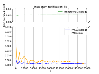
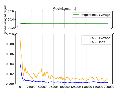
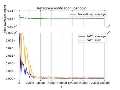
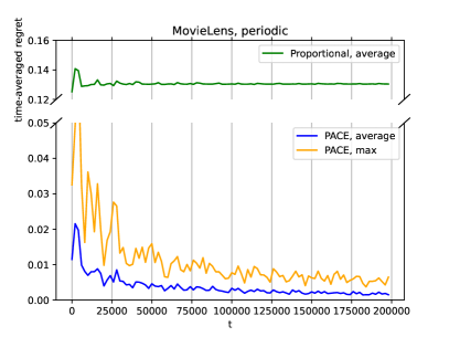
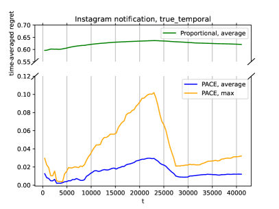
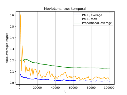
Figure 1: Simulations of PACE on the Instagram notification dataset (left) and the MovieLens dataset (right), under three types of inputs models: stationary (top), periodic (middle), and true temporal (bottom).

Results

For each of the three input models, we compute agents’ relative time-averaged regret at each time step. Letting $u_{i}^{*,1:\tau}$ be the utilities from the hindsight equilibrium, given all item appearances up to timestep $\tau$, the relative time-averaged regret is defined as

$$\text{relative time-averaged regret of $i$ at time $\tau$}:=\frac{\max\{u_{i}^{*,1:\tau}-\bar{u}_{i}^{\tau},0\}}{u_{i}^{*,1:\tau}},$$

In the plot, we show both the maximum value (labeled as “PACE, max”) and the arithmetic mean (labeled as “PACE, average”) of relative time-averaged regret across all $n$ agents. For comparison, we also plot the average relative regret given by simple proportional allocation which divides all items equally, labeled as “proportional, average”. For stochastic simulations, the plots show the average results of $10$ independent repetitions using different random seeds. The results are displayed in Figure 1.

For i.i.d. inputs, we see that PACE converges quickly numerically. Within a few iterations, its deviation falls within 1% of the current hindsight optimal utilities. After $t_{1}=200,000$ iterations, the relative average regret falls within 0.2% for all agents. For periodic inputs, despite the fluctuations caused by nonstationarity, the (relative) time-averaged regret also decreases to a very low level.

In the experiments with true temporal input, PACE suffers from larger deviation compared to stochastic and periodic input. However, at the end of the true temporal arrivals, it still attains an allocation where every agent is within $5$% of their hindsight equilibrium utility. We will next look more closely at the true temporal input for the Instagram dataset, which we will see displays extremely nonstationary behavior.

Figure 2 shows the time-averaged utility for each of the four notification types in the dataset. We see that the time-averaged utility fluctuates a lot, even for the hindsight optimal equilibrium utilities. In spite of this fluctuation, PACE tracks the hindsight-optimal utility closely. We now look at where in the original data this nonstationarity comes from. To do so, we plot the cumulative sum of each notification type’s value. As shown in Figure 3, agents’ values are distributed across the horizon in a highly non-uniform pattern. Remarkably, for the “liked” notification type, there is no positive-valued items from time $8,000$ until time $23,000$; this type of nonstationarity is highly undesirable for online algorithms. Despite the gap caused by the absence of “liked” notification opportunities, PACE is able to recover in the second half of the sequence, tracking the optimal solution closely.

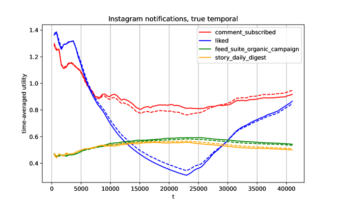
Figure 2: Time-averaged utility of each agent in true temporal experiments with Instagram notification dataset of PACE (solid line) and the optimal allocation given only the arrivals up to current timestep (dotted line)

.

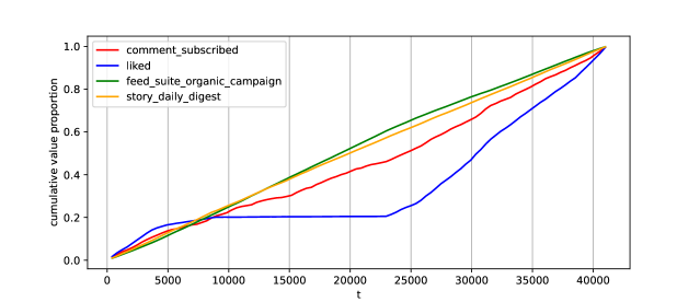
Figure 3: The cumulative value proportion (the fraction of the monopolistic utility of an agent revealed up to current step) of each agent in the true temporal Instagram notification arrival.

Appendix 0.A More on the Preliminaries

0.A.1 Review of Linear Fisher Market

In fair division the goal is to perform this allocation in a fair way, while simultaneously also guaranteeing some form of efficiency, typically Pareto efficiency. In the offline setting of allocating $m$ divisible goods to $n$ agents, the competitive equilibrium from equal incomes (CEEI) solution gives many efficiency and fairness guarantees. In CEEI, every agent is endowed with a unit budget of faux currency, a competitive equilibrium is computed, i.e., a set of item prices along with an allocation that clears the market, and the resulting allocation is used as the fair allocation [Varian, 1974]. This guarantees several fairness desiderata such as envy-freeness (every agent prefers his own bundle to that of any other person), proportionality (every agent prefers his own bundle over receiving their proportionally fair share of every item), and Pareto-optimality (we cannot make any person better off without making at least one other person worse off).

A linear Fisher market can be described as a tuple $\mathsf{F}=(n,m,B,\gamma)$, which consists of $n$ buyers and $m$ items. Each agent has budget $B_{i}>0$. Each item has unit supply. $\gamma=(v_{1},\cdots,v_{n})\in\left(\mathbb{R}_{+}^{m}\right)^{n}$ is a matrix of valuations, with $v_{i}^{j}$ being the valuation of item $j$ from buyer $i$. For buyer $i$, an allocation of item $x_{i}\in\mathbb{R}_{m}^{+}$ gives a utility of $u_{i}(x_{i}):=\langle v_{i},x_{i}\rangle=\sum_{j=1}^{m}v_{i}^{j}x_{i}^{j}$. Each item has a unit price $p^{j}\in\mathbb{R}_{+}$, and each buyer cannot overspend the budget, i.e., $\sum_{j=1}^{m}p^{j}x_{i}^{j}\leq B_{i}$. Note that the notations in this subsection for Fisher market is independent from those used in the paper body for online fair allocation.

Definition 2 (Demand).

Given item prices $p\in\mathbb{R}_{+}^{m}$, the demand of buyer $i$ is its set of utility-maximizing allocations given the prices and budget:

$$D_{i}(p)=\arg\max\left\{\langle v_{i},x_{i}\rangle:x_{i}\geq 0,\langle p,x_{i}\rangle\leq B_{i}\right\}.$$ (23)

Definition 3 (Market equilibrium).

The market equilibrium of $\mathsf{F}=(n,m,B,\gamma)$ is an allocation-price pair $(x^{*},p^{*})\in\left(\mathbb{R}_{+}^{m}\right)^{n}\times\mathbb{R}_{+}^{m}$ such that the following holds.

• Supply feasibility: $\sum_{i=1}^{n}x_{i}^{*}\leq 1_{m}$.

• Buyer optimality: $x_{i}^{*}\in D_{i}(p^{*})$ for all $i\in[n]$.

• Market clearance: $\langle p^{*},1_{m}-\sum_{i=1}^{n}x_{i}^{*}\rangle=0$.

Market equilibrium and fair allocation are closely related. We can give translate a fair division instance into Fisher market by assigning each agent’s budget of faux currency according to their weight $B_{i}$. By computing what is called a market equilibrium under this new market, we can use the corresponding Fisher market allocation as the fair division output.

It is known that a CEEI allocation $x^{*}$ has many desirable properties. It is Pareto optimal (every market equilibrium is Pareto optimal by the first welfare theorem). It is envy-free, since each agent has the same budget in CEEI and every agent is buying something in his demand set and each can afford the bundle of any other agent. Finally, proportionality is satisfied, since each agent can afford the bundle where they get a proportional share of each good.

The market equilibrium is essentially a collection of optimization problems as in (23) coupled by the supply feasibility constraint. A celebrated result is the Eisenberg-Gale convex program, which provides an equivalent characterization of Fisher market equilibrium:

$$\max_{x_{1},\cdots,x_{n}}\sum_{i=1}^{n}B_{i}\log\langle v_{i},x_{i}\rangle\ \ \textnormal{s.t.}\sum_{i=1}^{n}x_{i}^{j}\leq 1\ \ \ \forall j\in[m],\ \ x_{i}\in\mathbb{R}_{+}^{m}\ \ \ \forall i\in[n].$$

That is, we maximize the sum of logarithmic utilities under the supply constraint. The solution to the primal problem $x^{*}=(x_{1}^{*},\cdots,x_{n}^{*})$ along with the vector of dual variables $p^{*}$ gives a Fisher market equilibrium.

0.A.2 The Dual of EG and its infinite-dimensional analogue

We next show how to derive the dual problem (2) from the primal problem (1). Introduce the dual variables $\beta_{i}\geq 0$ with $i\in[n]$ for each constraint of the first type and variables $p^{\tau}\geq 0$ with $\tau\in[t]$ for constraints of the second type. The Lagrangian $L:\mathbb{R}_{+}^{n\times t}\times\mathbb{R}_{+}^{n}\times\mathbb{R}_{+}^{n}\times\mathbb{R}_{+}^{t}\rightarrow\mathbb{R}$ is given by

$$L(x,U,\beta,p) =\sum_{i=1}^{n}B_{i}\log U_{i}+\sum_{i=1}^{n}\beta_{i}\left(\langle v_{i},x_{i}\rangle-U_{i}\right)+\sum_{\tau=1}^{t}p^{\tau}\left(1-\sum_{i=1}^{n}x_{i}^{\tau}\right)$$

$$=\sum_{\tau=1}^{t}p^{\tau}+\sum_{i=1}^{n}\left(B_{i}\log U_{i}-\beta_{i}U_{i}\right)+\sum_{i=1}^{n}\langle\beta_{i}v_{i}-p,x_{i}\rangle.$$

Maximizing over the primal variables $(x,U)$ gives the dual program

$$\min_{p\geq 0,\beta\geq 0}\left\{\left.\sum_{\tau=1}^{t}p^{\tau}-\sum_{i=1}^{n}B_{i}\log\beta_{i}+\sum_{i=1}^{n}(B_{i}\log B_{i}-B_{i})\right|p\geq\beta_{i}v_{i},\forall i\in[n]\right\}.$$

Ignoring the constants and moving the constraint $p\geq\beta_{i}v_{i}$ to the criterion, we obtain the following equivalent optimization problem, which is exactly (2).

$$\min_{\beta\geq 0}\left\{\sum_{\tau=1}^{t}\max_{i\in[n]}\beta_{i}v_{i}^{\tau}-\sum_{i=1}^{n}B_{i}\log\beta_{i}\right\}.$$

Consider the infinite-dimensional analogue of Eisenberg-Gale program (3),

$$\max_{x\in L^{\infty}_{+}(V),u\geq 0}\left\{\left.\sum_{i=1}^{n}B_{i}\log u_{i}\ \right|\ u_{i}\leq\langle v_{i},x_{i}\rangle\ \forall i\in[n],\ \sum_{i=1}^{n}x_{i}\leq s\right\}.$$

We can derive its dual problem, which is the infinite-dimensional analogue of (2),

$$\min_{\beta\geq 0}\left\{\int_{V}\left(\max_{i\in[n]}\beta_{i}v_{i}\right)\mathrm{d}\bar{Q}-\sum_{i=1}^{n}B_{i}\log\beta_{i}\right\}.$$

The relationship between the two versions of the dual program is that we replaced the uniform averaging over samples in (2) with an integral w.r.t. the value distribution $\bar{Q}$ in (4). When the value space is continuous, the supply, allocation and pricing functions are measurable functions over the space in (4), which can be infinite-dimensional. In the stochastic case where item arrivals are drawn from a distribution with density $s$, they correspond to an underlying market with item supply $s$; the underlying dual program will serve as the reference programs that facilitate the analyze of dual convergence and regret. The rigorous mathematical treatment of infinite-dimensional markets can be found in Gao and Kroer [2023], Gao et al. [2021].

0.A.3 Interpretation from PACE to Dual Averaging

Next we show how to cast PACE as dual averaging applied to the problem (2). As we have discussed, although PACE has exactly the same operations as dual averaging on (2), any existing results for dual averaging cannot be applied directly, since it lacks the property of boundedness and strong convexity. In our problem we have

$$F(\beta,v^{\tau}) =f(\beta,v^{\tau})+\Psi(\beta),$$

$$f(\beta,v^{\tau}) =\max_{i}\beta_{i}v_{i}^{\tau},$$

$$\Psi(\beta) =-\sum_{i=1}^{n}B_{i}\log\beta_{i}.$$

Notice that, different from the presentation of dual averaging by Xiao [2009], for our problem we do not need an additional external regularizer; $\Psi(\beta)$ is part of the dual objective. Since $f(\cdot,v^{\tau})$ is a piecewise linear function, a subgradient is

$$g^{\tau}=v_{i^{\tau}}^{\tau}e_{i^{\tau}}\in\partial_{\beta}f(\beta,v^{\tau}),$$

where $i^{\tau}=\min\arg\max_{i}\beta_{i}v_{i}^{\tau}$ is the index of the winning agent. We notice that by PACE’s integral allocation, we have $g_{i}^{\tau}=v_{i}^{\tau}\mathbb{I}\{i=i^{\tau}\}=v_{i}^{\tau}x_{i}^{\tau}=u_{i}^{\tau}$. Hence, the subgradient $g^{\tau}$ coincides with PACE’s resulting instantaneous utility at time step $\tau$.

We elaborate on the correspondence of each step of PACE to dual averaging:

• (1) Subgradient computation: $g^{\tau}=u^{\tau}$.

• (2) Average subgradient: $\bar{g}^{\tau}=\bar{u}^{\tau}=\frac{\tau-1}{\tau}\bar{u}^{\tau-1}+\frac{1}{\tau}u^{\tau}$.

• (3) Solve the regularized problem:

  $$\beta^{\tau+1}=\arg\min\left\{\left.\langle\bar{g}^{\tau},\beta\rangle-\sum_{i=1}^{n}B_{i}\log\beta_{i}\right|\beta\geq 0\right\}\implies\beta_{i}^{\tau+1}=\frac{B_{i}}{\bar{u}_{i}^{\tau}}.$$

0.A.4 Inputs that Cause Failure of Constrained PACE

We show that the constrained version of PACE algorithm [Gao et al., 2021, Liao et al., 2022] is vulnerable either when 1) the input value is adversarially chosen, or 2) agent values and budgets are not normalized in the stochastic case. It turns out that simple adversarial construction result in the constrained algorithm allocating nothing to one of the agent at all, even when the hindsight optimal allocation is a equal division.

The constrained PACE algorithm is similar to Algorithm 1, the only difference being it projects the pacing multiplier to a fixed interval at each time-step:

$$\beta_{i}^{\tau+1}=\mathrm{Proj}_{\left[\frac{B_{i}}{1+\delta_{0}},(1+\delta_{0})\right]}\frac{B_{i}}{\bar{u}_{i}^{\tau}}.$$

We show that, the projection causes the failure of the algorithm for any fixed (independent of $t$) target interval $[\ell_{i},r_{i}]$, where $0\leq\ell_{i}<r_{i}<\infty$ .

Example 2.

Consider 2-agent instances with equal weights $B_{1}=B_{2}=1$. For constrained PACE algorithm that projects agent multipliers to $[\ell_{1},r_{1}]$, $[\ell_{2},r_{2}]$ (assuming $r_{2}\leq r_{1}$ without loss of generality), consider the following input instance:

$$v_{1}^{\tau}=v_{2}^{\tau}=\min\left\{\frac{1}{r_{2}},\|v\|_{\infty}\right\},\ \forall\tau\in[t].$$

Then for constrained PACE, clearly we have for every time step,

$$\beta_{1}^{\tau+1}=\beta_{2}^{\tau+1}=r_{2},\ \forall\tau\in[t].$$

Every item is allocated to agent $1$; agent $2$ has final utility $0$.

Example 2 can be regarded both as an adversarially constructed input, or as a stationary input where each round is i.i.d. with the distribution being degenerate. In fact, a fixed upper bound in the projection interval of constrained PACE requires prior knowledge or normalization on $B_{i}$ and agent values; otherwise it is easily corrupted otherwise by such simple instances as Example 2.

Appendix 0.B Missing Proofs in Section 5

0.B.1 Proof of Lemma 1

See 1

0.B.1.1 Conjugate Function $V^{t}(w)$ and Its Properties.

Notice that $\Psi(\beta)$ is monotonically decreasing on each $\beta_{i}$. We have

$$h=(h_{1},\cdots,h_{n})=\arg\min_{\beta\in\mathcal{F}_{h}}\Psi(\beta).$$

Define $w^{t}:=\sum_{\tau=1}^{t}g^{\tau}$ to be the sum of gradients up to time step $t$. For each $t\geq s$, we consider a conjugate-type function:

$$V^{t}(w)=\max_{\beta\in\mathcal{F}_{h}}\left\{\langle w,\beta-h\rangle-t\Psi(\beta)\right\}.$$

By comparing the definition $V^{t}(w)$ and the update rule of $\beta$, we have for any $t\geq s-1$,

$$\beta^{t+1}=\arg\min_{\beta>0}\left\{\langle w^{t},\beta\rangle+t\Psi(\beta)\right\}\overset{\text{(a)}}{=}\arg\min_{\beta\in\mathcal{F}_{h}}\left\{\langle w^{t},\beta\rangle+t\Psi(\beta)\right\}=\arg\max_{\beta\in\mathcal{F}_{h}}V^{t}(-w^{t}),$$ (24)

where (a) is by the definition of the event $A_{h,s}$.

For any $t\geq s$, $\Psi(\beta)$ is strongly convex on the domain $\mathcal{F}_{h}$, which is non-empty and closed. Therefore, the maximum is always achieved, and the maximizer is unique. Also, by $\Psi(h)\leq 0$, the function $V^{t}(w)$ is always non-negative.

Let $\pi^{t}(w)$ denote the unique maximizer in the definition of $V^{t}(w)$. We have

$$\pi^{t}(w) =\arg\max_{\beta\in\mathcal{F}_{h}}\left\{\langle w,\beta-h\rangle-t\Psi(\beta)\right\}$$

$$=\arg\min_{\beta\in\mathcal{F}_{h}}\left\{\langle-w,\beta\rangle+t\Psi(\beta)\right\}$$

Combined with (24), we have

$$\beta^{t+1}=\pi^{t}(-w^{t}),\ \ \forall t\geq s-1.$$

Lemma 6.

The function $V^{t}(w)$ is convex and differentiable. Its gradient is given by

$$\nabla V^{t}(w)=\pi^{t}(w)-h.$$ (25)

Moreover, the gradient is Lipschitz continuous with parameter $1/\sigma t$, i.e.,

$$\|\nabla V^{t}(w_{1})-\nabla V^{t}(w_{2})\|\leq\frac{1}{\sigma t}\|w_{1}-w_{2}\|_{*},\ \ \forall w_{1},w_{2}\geq 0.$$

The proof of Lemma 6 follows from classical results of convex analysis, see, for example, Boyd and Vandenberghe [2004]. $\hfill\square$

A direct consequence of the Lipschitz gradients result in Lemma 6 is the following inequality:

$$V^{t}(w+g)\leq V^{t}(w)+\langle g,\nabla V^{t}(w)\rangle+\frac{1}{2\sigma t}\|g\|_{*}^{2},\ \ \forall w,g\geq 0.$$ (26)

Lemma 7.

For each $t\geq s$, we have

$$V^{t}(-w^{t})+\Psi(\beta^{t+1})\leq V^{t-1}(-w^{t}).$$

Proof of Lemma 7.

By the definition of $V^{t-1}(-w^{t})$,

$$V^{t-1}(-w^{t}) =\max_{\beta\in\mathcal{F}_{h}}\left\{\langle-w^{t},\beta-h\rangle-(t-1)\Psi(\beta)\right\}$$

$$\geq\langle-w^{t},\beta^{t+1}-h\rangle-(t-1)\Psi(\beta^{t+1})$$

$$=\left\{\langle-w^{t},\beta^{t+1}-h\rangle-t\Psi(\beta^{t+1})\right\}+\Psi(\beta^{t+1})$$

$$=V^{t}(-w^{t})+\Psi(\beta^{t+1}),$$

where the last step is due to (24). $\hfill\square$

With these lemmas in hand, we proceed with the proof of Lemma 1.

0.B.1.2 Bounding the Primal Variable.

By the optimality condition for the decision rule of PACE , there exists a subgradient $d^{t+1}\in\partial\Psi(\beta^{t+1})$ such that

$$\langle w^{t}+td^{t+1},\beta-\beta^{t+1}\rangle\geq 0,\ \forall\beta>0.$$ (27)

Consider $t\geq s$. By the strong convexity of $\Psi(\beta)$ on $\mathcal{F}_{h}$,

$$\Psi(\beta)\geq\Psi(\beta^{t+1})+\langle d^{t+1},\beta-\beta^{t+1}\rangle+\frac{\sigma^{2}}{2}\|\beta-\beta^{t+1}\|^{2},\ \ \forall\beta>0,t\geq s.$$ (28)

By multiplying both sides of (28) by $t$ and rearranging terms, we have for $t\geq s$,

$$\frac{\sigma t}{2}\|\beta-\beta^{t+1}\|^{2}\leq-\langle td^{t+1},\beta-\beta^{t+1}\rangle+t\Psi(\beta)-t\Psi(\beta^{t+1}).$$

Using the optimality condition (27), we have for $t\geq s$,

$$\frac{\sigma t}{2}\|\beta-\beta^{t+1}\|^{2} \leq\langle w^{t},\beta-\beta^{t+1}\rangle+t\Psi(\beta)-t\Psi(\beta^{t+1})$$

$$=\left\{\langle-w^{t},\beta^{t+1}-h\rangle-t\Psi(\beta^{t+1})\right\}+t\Psi(\beta)+\langle w^{t},\beta-h\rangle$$

$$=V^{t}(-w^{t})+t\Psi(\beta)+\langle w^{t},\beta-h\rangle.$$

Now we expand the last term on the right hand side, and split the horizon at round $s$,

$$\frac{\sigma t}{2}\|\beta-\beta^{t+1}\|^{2} \leq V^{t}(-w^{t})+t\Psi(\beta)+\sum_{\tau=1}^{t}\langle g^{\tau},\beta-h\rangle$$

$$=V^{t}(-w^{t})+t\Psi(\beta)+\sum_{\tau=1}^{s}\langle g^{\tau},\beta-h\rangle+\sum_{\tau=s+1}^{t}\langle g^{\tau},\beta-h\rangle$$

$$=V^{t}(-w^{t})+t\Psi(\beta)+\sum_{\tau=1}^{s}\langle g^{\tau},\beta-h\rangle+\sum_{\tau=s+1}^{t}\langle g^{\tau},\beta-\beta^{\tau}\rangle+\sum_{\tau=s+1}^{t}\langle g^{\tau},\beta^{\tau}-h\rangle$$

By further adding and subtracting $\sum_{\tau=s+1}^{t}\Psi(\beta^{\tau})$ to the right-hand side, the inequality becomes

$$\frac{\sigma t}{2}\|\beta-\beta^{t+1}\|^{2}\leq \underbrace{\sum_{\tau=s+1}^{t}\langle g^{\tau},\beta-\beta^{\tau}\rangle+(t-s)\Psi(\beta)-\sum_{\tau=s+1}^{t}\Psi(\beta^{\tau})}_{\text{(I)}}$$

$$+ \underbrace{\sum_{\tau=1}^{s}\langle g^{\tau},\beta-h\rangle+s\Psi(\beta)}_{\text{(II)}}$$

$$+ \underbrace{V^{t}(-w^{t})+\sum_{\tau=s+1}^{t}\left(\langle g^{\tau},\beta^{\tau}-h\rangle+\Psi(\beta^{\tau})\right)}_{\text{(III)}}.$$

Next, we bound the three terms (I), (II), and (III), respectively.

0.B.1.3 Bounding Term (I).

Term (I) can be rearranged into the negative regret over rounds $s+1,\ldots,t$. By convexity of $f(\cdot,v^{\tau})$,

(I) $$=\sum_{\tau=s+1}^{t}\langle g^{\tau},\beta-\beta^{\tau}\rangle+(t-s)\Psi(\beta)-\sum_{\tau=s+1}^{t}\Psi(\beta^{\tau})$$

$$\leq\sum_{\tau=s+1}^{t}\left(f(\beta,v^{\tau})-f(\beta^{\tau},v^{\tau})\right)+(t-s)\Psi(\beta)-\sum_{\tau=s+1}^{t}\Psi(\beta^{\tau})$$

$$=-\textnormal{Dual-Regret}(s,\beta).$$

0.B.1.4 Bounding Term (II).

Recall that in our problem $g_{i}^{\tau}=u_{i}^{\tau}\leq\|v_{i}\|_{\infty}$ for each $i$. Then,

$$\text{(II)}=\sum_{\tau=1}^{s}\langle g^{\tau},\beta-h\rangle+s\Psi(\beta)\leq-\sum_{\tau=1}^{s}\langle g^{\tau},h\rangle+s\cdot\left(\max_{i}\beta_{i}\|v_{i}\|_{\infty}-\sum_{i}B_{i}\log\beta_{i}\right)$$

0.B.1.5 Bounding Term (III).

For any $\tau\geq s+1$, we have

$$V^{\tau}(-s^{\tau})+\Psi(\beta^{\tau+1}) \overset{\text{(a)}}{\leq}V^{\tau-1}(-s^{\tau})$$

$$=V^{\tau-1}(-s^{\tau-1}-g^{\tau})$$

$$\overset{\text{(b)}}{\leq}V^{\tau-1}(-s^{\tau-1})+\langle-g^{\tau},\nabla V^{\tau-1}(-s^{\tau-1})\rangle+\frac{\|g^{\tau}\|^{2}_{*}}{2\sigma(\tau-1)}$$

$$\overset{\text{(c)}}{=}V^{\tau-1}(-s^{\tau-1})+\langle-g^{\tau},\beta^{\tau}-h\rangle+\frac{\|g^{\tau}\|^{2}_{*}}{2\sigma(\tau-1)},$$

where the steps (a), (b), and (c) are due to Lemma 7, (26), and (25), respectively. Rearranging the terms, we have

$$\langle g^{\tau},\beta^{\tau}-h\rangle+\Psi(\beta^{\tau+1})\leq V^{\tau-1}(-s^{\tau})-V^{\tau}(-s^{\tau})+\frac{\|g^{\tau}\|^{2}_{*}}{2\sigma(\tau-1)},\ \ \forall\tau\geq s+1.$$

Summing the inequalities from $\tau=s+1,\cdots,t$, we have

(III) $$=\sum_{\tau=s+1}^{t}\left(\langle g^{\tau},\beta^{\tau}-h\rangle+\Psi(\beta^{\tau+1})\right)+V^{t}(-w^{t})$$

$$\leq V^{s}(-w^{s})+\frac{1}{2}\sum_{\tau=s+1}^{t}\frac{\|g^{\tau}\|^{2}_{*}}{\sigma(\tau-1)}$$

$$=\langle-w^{s},\beta^{s+1}-h\rangle-s\Psi(\beta^{s+1})+\frac{1}{2}\sum_{\tau=s+1}^{t}\frac{\|g^{\tau}\|^{2}_{*}}{\sigma(\tau-1)}$$

$$\leq\sum_{\tau=1}^{s}\langle g^{\tau},h\rangle+s\sum_{i=1}^{n}B_{i}\log h_{i}+\frac{1}{2}\sum_{\tau=s+1}^{t}\frac{\|g^{\tau}\|^{2}_{*}}{\sigma(\tau-1)}$$

Putting Everything Together

Combining the bounds for term (I), (II), and (III),

$$\frac{\sigma t}{2}\|\beta-\beta^{t+1}\|^{2}\leq\frac{1}{2}\sum_{\tau=s+1}^{t}\frac{\|g^{\tau}\|^{2}_{*}}{\sigma(\tau-1)}+\left(\max_{i}\beta_{i}\|v_{i}\|_{\infty}+\sum_{i}B_{i}\log\frac{h_{i}}{\beta_{i}}\right)\cdot s-\textnormal{Dual-Regret}(s,\beta).$$ (29)

We also have

$$\frac{1}{2}\sum_{\tau=s+1}^{t}\frac{\|g^{\tau}\|^{2}_{*}}{\sigma(\tau-1)}<\frac{\max_{\tau}\|g^{\tau}\|_{*}^{2}}{2\sigma}\log t\leq\frac{\max_{i}\|v_{i}\|_{\infty}^{2}}{2\sigma}\log t.$$ (30)

Combining (29) and (30), we have

$$\frac{\sigma t}{2}\|\beta-\beta^{t+1}\|^{2}\leq\frac{\max_{i}\|v_{i}\|_{\infty}^{2}}{2\sigma}\log t+\left(\max_{i}\beta_{i}\|v_{i}\|_{\infty}+\sum_{i}B_{i}\log\frac{h_{i}}{\beta_{i}}\right)\cdot s-\textnormal{Dual-Regret}(s,\beta).$$

Multiplying both sides by ${2}/{\sigma t}$, we arrive at

$$\|\beta-\beta^{t+1}\|^{2}\leq\frac{2}{\sigma t}\left(\frac{\max_{i}\|v_{i}\|_{\infty}^{2}}{2\sigma}\log t+\left(\max_{i}\beta_{i}\|v_{i}\|_{\infty}+\sum_{i}B_{i}\log\frac{h_{i}}{\beta_{i}}\right)\cdot s-\textnormal{Dual-Regret}(s,\beta)\right).$$

This proves Lemma 1.

0.B.2 Proof of Lemma 2.

See 2 For $\tau>s$, we decompose the dual regret at time $\tau$ as follows,

$$F(\beta^{\tau},v^{\tau})-F(\beta^{*},v^{\tau})=\underbrace{\left(F(\beta^{\tau},v^{\tau})-\phi(\beta^{\tau})\right)}_{\text{(I)}}+\underbrace{\left(\phi(\beta^{*})-F(\beta^{*},v^{\tau})\right)}_{\text{(II)}}+\underbrace{\left(\phi(\beta^{\tau})-\phi(\beta^{*})\right)}_{\text{(III)}}.$$ (31)

By the optimality of $\beta^{*}$ we have $\text{(III)}\geq 0$ always. Next, we bound (I) and (II).

Let $\hat{Q}$ be the distribution of $v|A_{h,s}$, $\hat{Q}^{1:\tau}$ be the marginal distribution of $\hat{Q}$ on the first $\tau$ rounds, and $\hat{Q}^{\tau}(\cdot|v^{1:\tau-1})$ be the distribution of $v^{\tau}$ conditioned on $A_{h,s}$ and the information of previous rounds.

Note that

$$\mathbb{E}\left[\text{(I)}|A_{h,s}\right]=\mathbb{E}_{v^{1:\tau-1}\sim\hat{Q}^{1:\tau-1}}\left[\mathbb{E}_{v^{\tau}\sim\hat{Q}^{\tau}}\left[\left(F(\beta^{\tau},v^{\tau})-\phi(\beta^{\tau})\right)\mid v^{1:\tau-1}\right]\right].$$

Let us investigate the inner expectation. Conditional on $v^{1:\tau-1}$, the pacing multiplier $\beta^{\tau}$ is deterministic.

$$\left|\mathbb{E}_{v^{\tau}\sim\hat{Q}^{\tau}}\left[\left(F(\beta^{\tau},v^{\tau})-\phi(\beta^{\tau})\right)\mid v^{1:\tau-1}\right]\right| \leq\mathbb{E}_{v^{\tau}\sim\hat{Q}^{\tau}}\left[\left|F(\beta^{\tau},v^{\tau})-\phi(\beta^{\tau})\right|\mid v^{1:\tau-1}\right]$$

$$=\left|\int_{0}^{\|v\|_{\infty}}F(\beta^{\tau},v)\hat{Q}^{\tau}(\mathrm{d}v|v^{1:\tau-1})-\int_{0}^{\|v\|_{\infty}}F(\beta^{\tau},v)\mathrm{d}\bar{Q}(v)\right|$$

$$\leq G(h)\int_{0}^{\|v\|_{\infty}}\left|\mathrm{d}\hat{Q}^{\tau}(\cdot|v^{1:\tau-1})-\mathrm{d}\bar{Q}(v)\right|$$

$$=2G(h)\cdot\|\hat{Q}^{\tau}(\cdot|v^{1:\tau-1})-\bar{Q}(\cdot)\|_{\mathrm{TV}}.$$ (32)

Next, we deal with the outer expectation. Let $\hat{\mathcal{V}}^{\tau}$ be the support of $\hat{Q}^{\tau}(\cdot\mid v^{1:\tau-1})$. Since $\hat{Q}^{\tau}$ is also conditioned on $A_{h,s}$, we have

$$v^{1:\tau-1}\not\in\hat{\mathcal{V}}^{\tau}\implies\Pr[A_{h,s}|v^{1:\tau-1}]=0.$$

Hence,

$$\Pr[A_{h,s}]\leq\mathbb{E}_{v^{1:\tau-1}\sim\hat{Q}^{1:\tau-1}}\left[\Pr[A_{h,s}\mid v^{1:\tau-1}\right]+\Pr[A_{h,s}\mid v^{1:\tau-1}\not\in\hat{\mathcal{V}}^{\tau}] =\mathbb{E}_{v^{1:\tau-1}\sim\hat{Q}^{1:\tau-1}}\left[\Pr[A_{h,s}\mid v^{1:\tau-1}\right]$$ (33)

We can use a failure probability term to bound (I) as follows,

$$\mathbb{E}\left[|\text{(I)}||A_{h,s}\right] \leq\mathbb{E}_{v^{1:\tau-1}\sim\hat{Q}^{1:\tau-1}}\left[\left|\mathbb{E}_{v^{\tau}\sim\hat{Q}^{\tau}}\left[\left(F(\beta^{\tau},v^{\tau})-\phi(\beta^{\tau})\right)\mid v^{1:\tau-1}\right]\right|\right]$$

$$\leq 2G(h)\cdot\mathbb{E}_{v^{1:\tau-1}\sim\hat{Q}^{1:\tau-1}}\left[\|\hat{Q}^{\tau}(\cdot|v^{1:\tau-1})-\bar{Q}(v)\|_{\mathrm{TV}}\right]$$

$$=2G(h)\cdot\mathbb{E}_{v^{1:\tau-1}\sim\hat{Q}^{1:\tau-1}}\left[\|Q^{\tau}\left(\cdot|A_{h,s},v^{1:\tau-1}\right)-\bar{Q}(v)\|_{\mathrm{TV}}\right]$$

$$\overset{\text{(a)}}{\leq}2G(h)\cdot\mathbb{E}_{v^{1:\tau-1}\sim\hat{Q}^{1:\tau-1}}\left[1-\Pr\left[A_{h,s}\mid v^{1:\tau-1}\right]\right]$$

$$\overset{\text{(b)}}{\leq}2G(h)\cdot\left(1-\Pr\left[{A_{h,s}}\right]\right),$$ (34)

where (a) is by the property of total variation distance that $\|Q^{\tau}(\cdot|A)-\bar{Q}(\cdot)\|_{\mathrm{TV}}\leq(1-\Pr[A])$ for any measurable event $A$, and (b) is by (33).

Next we bound $\mathbb{E}\left[|\text{(II)}||A_{h,s}\right]$. Notice that similar analysis goes through without the outer expectation.

$$\mathbb{E}\left[|\text{(II)}||A_{h,s}\right]\leq 2\bar{F}(\beta^{*})(1-\Pr[A_{h,s}])$$ (35)

Combining (I), (II), and $\text{(III)}>0$ and summing over $\tau=s+1,\cdots,t$, we prove Lemma 2.

0.B.3 Proof of Lemma 3

See 3 For agent $j$, let $T_{j}:=\{\tau\in[t]:x_{j}^{\tau}=1\}$ be the index set of items that are allocated to agent $j$ in PACE. For i.i.d. inputs, we denote $\mu_{j}:=\mathbb{E}[v_{i}^{\tau}]$. We are going to show that, for each $j\in[n]$ there exists $u_{j}^{\prime}=\Omega(1/n)$ (which is independent of $t$), and constant $c_{1},c_{2}>0$ (which are independent of both $t$ and $n$), such that

$$\Pr[\bar{u}_{j}^{\tau}<u_{j}^{\prime}]=O\left(e^{-c_{1}\tau/n}\right),\ \forall\tau>c_{2}n.$$ (36)

We first show how (36) leads to Lemma 3. By (36) and the fact that $c_{1}$ is independent of $n$, we know that the sum of $\Pr[\bar{u}_{j}^{\tau}<u_{j}^{\prime}]$ over $\tau\geq s$ can be bounded by the sum of geometric series, where $s>c_{2}n$,

$$\sum_{\tau\geq s}\Pr[\bar{u}_{j}^{\tau}<u_{j}^{\prime}]=O\left(e^{-c_{1}s/n}\right).$$

By union bound over $j\in[n]$ and $\tau\geq s$,

$$\Pr\left[\exists\tau\geq s,j\in[n],\ \ \bar{u}_{j}^{\tau}<u_{j}^{\prime}\right]=O\left(n^{2}e^{-c_{1}s/n}\right),\ s>c_{2}n.$$

Since we have $\beta_{j}^{\tau}\geq B_{j}/\|v_{j}\|_{\infty}$ always,

$$\forall\tau\geq s,j\in[n],\bar{u}_{j}^{\tau}\geq u_{j}^{\prime}\implies A_{h,s},\ \left(h_{j}=B_{j}/u_{j}^{\prime}=O(n)\right).$$

Hence for $h=(h_{1},\cdots,h_{n}),$ where $h_{j}=B_{j}/u_{j}^{\prime}$,

$$1-\Pr\left[A_{h,s}\right]=O\left(n^{2}e^{-c_{1}s/n}\right),\ s>c_{2}n.$$

Choosing $\hat{s}(t,n)=\max\{c_{2}n+1,c_{1}^{-1}n(\log n+\log t)\}$ will result in an $O(n/t)$ failure probability, which shows Lemma 3.

The rest of the proof is devoted to showing (36).

0.B.3.1 Bounding the monopolistic utility.

Consider $j\in[n]$, and the following event

$$X:=\left\{\gamma:\sum_{t^{\prime}=1}^{\tau}v_{j}^{t^{\prime}}>\left(\mu_{j}-\Delta_{j}\right)\tau\right\},$$

which characterizes a lower bound of his monopolistic utility (sum of values for all items so far) at time step $\tau.$ By Hoeffding bounds, we can show a high probability bound for $X$,

$$\Pr\left[X^{c}\right]\leq\exp\left(-\frac{2\Delta_{j}^{2}\tau}{\|v_{j}\|_{\infty}^{2}}\right),\ \forall\Delta_{j}>0.$$ (37)

Notice that

$$X\implies\sum_{t^{\prime}\not\in T_{j}}v_{j}^{t^{\prime}}>\left(\mu_{j}-\Delta_{j}-\bar{u}_{j}^{\tau}\right)\tau.$$

For $\lambda>0$, let $M_{j}(\lambda)$ be the index set of items which agent $j$ has valuation at least $\lambda$ and was not allocated to agent $j$ by PACE. Define $m_{j}(\lambda)=|M_{j}(\lambda)|$. Then, by

$$\sum_{t^{\prime}\not\in T_{j}}v_{j}^{t^{\prime}}\leq m_{j}(\lambda)\|v_{j}\|_{\infty}+(\tau-m_{j}(\lambda))\lambda,$$

we have

$$X\implies m_{j}(\lambda)>\frac{\mu_{j}-\Delta_{j}-\bar{u}_{j}^{\tau}-\lambda}{\|v_{j}\|_{\infty}-\lambda}\cdot\tau.$$ (38)

0.B.3.2 Bounding competing agents’ utility.

Let $i=\min\arg\max_{k\neq j}|M_{j}(\lambda)\cap T_{k}|.$ Then, we have

$$|M_{j}(\lambda)\cap T_{i}|\geq\frac{m_{j}(\lambda)}{n}.$$

Let $r=\max\{M_{j}(\lambda)\cap T_{i}\}$. We consider the event

$$Y:=\left\{\gamma:U_{i}^{r}>(\mu_{i}-\Delta_{i})\frac{m_{j}(\lambda)}{n}\right\}.$$

By the definition of $T_{i}$, we have

$$U_{i}^{r}\geq\sum_{t^{\prime}\in M_{j}(\lambda)\cap T_{i}}v_{i}^{t^{\prime}}.$$ (39)

We know from the decision rule of PACE that for $t^{\prime}\in M_{j}(\lambda)\cap T_{i}$,

$$v_{i}^{t^{\prime}}\geq\max_{k\neq i}\left\{\frac{v_{j}^{t^{\prime}}U_{i}^{t^{\prime}-1}}{U_{j}^{t^{\prime}-1}}\right\}.$$

Therefore, the right hand side of (39) stochastically dominates $\sum_{t^{\prime}\in M_{j}(\lambda)\cap T_{i}}S_{i}^{t^{\prime}}$, where random variable $S_{i}^{t^{\prime}}:=v_{i}^{t^{\prime}}\mid v_{i}^{t^{\prime}}>0$ is defined as the per-round agent value conditioned on itself being nonzero. By Azuma-Hoeffding inequality, we have

$$\Pr\left[Y^{c}\right]\leq\Pr\left[\sum_{t^{\prime}\in M_{j}(\lambda)\cap T_{i}}v_{i}^{t^{\prime}}\leq\left(\mu_{i}-\Delta_{i}\right)\frac{m_{j}(\lambda)}{n}\right]\leq\exp\left(-\frac{2\Delta_{i}^{2}\cdot m_{j}(\lambda)}{n\cdot\|v_{i}\|_{\infty}^{2}}\right),\ \Delta_{i}>0.$$ (40)

0.B.3.3 Lower Bound for $\bar{u}_{j}^{\tau}$.

By the PACE decision rule on item $r$, it holds that

$$U_{i}^{r}-\|v_{i}\|_{\infty}\leq U_{i}^{r-1}\leq\frac{B_{i}U_{j}^{r-1}v_{i}^{r}}{B_{j}v_{j}^{r}}\leq\frac{B_{i}\|v_{i}\|_{\infty}\bar{u}_{j}^{\tau}}{B_{j}\lambda}\cdot\tau.$$ (41)

Combining (41) and the definition of $X$ and $Y$, we have

$$X\cap Y\implies\bar{u}_{j}^{\tau}\geq\frac{B_{j}\left(\mu_{j}-\Delta_{j}-\lambda-\frac{n\|v_{i}\|_{\infty}(\|v_{j}\|_{\infty}-\lambda)}{(\mu_{i}-\Delta_{i})\tau}\right)\lambda}{B_{j}\lambda+\frac{\|v_{i}\|_{\infty}B_{i}}{(\mu_{i}-\Delta_{i})}\cdot(\|v_{j}\|_{\infty}-\lambda)\cdot n}.$$ (42)

0.B.3.4 Fixing $\Delta$ and $\lambda$.

We now determine the values for $\Delta_{i},\Delta_{j},\lambda$, such that the right hand side of (42) gives us a meaningful bound. By choosing $\Delta_{i}=\mu_{i}/2$ and $\Delta_{j}=\lambda=\mu_{j}/4$, we have that for $\tau\geq\frac{8n\max_{k}\|v_{k}\|_{\infty}\|v_{j}\|_{\infty}}{\mu_{k}\mu_{j}}$,

$$\bar{u}_{j}^{\tau}\geq\bar{u}_{j}^{\prime}:=\min\left\{\frac{\mu_{j}}{4},\frac{B_{j}\mu_{j}^{2}}{4B_{j}\mu_{j}+32n\cdot(\|v_{j}\|_{\infty}-\mu_{j}/4)\cdot\max_{k}\left\{B_{k}\|v_{k}\|_{\infty}/\mu_{k}\right\}}\right\}\in\Omega\left(\frac{1}{n}\right).$$

The failure probability of above is at most $\Pr[X^{c}]+\Pr[Y^{c}]$, which is

$$\exp\left(-\frac{\mu_{j}^{2}}{8\|v_{j}\|_{\infty}^{2}}\tau\right)+\exp\left(-\frac{\min_{k}\mu_{k}^{2}\cdot\mu_{j}}{n\|v_{i}\|_{\infty}\cdot\left(8\|v_{j}\|_{\infty}-2\mu_{j}\right)}\cdot\tau\right)=O(e^{-c_{1}\tau/n}),$$

where $c_{1}$ is a constant independent of $n$ and $\tau$. This proves (36).

0.B.4 Proof of Theorem 5.3.

See 5.3 We show the following lemma, which reduces the question of spending convergence into a convergence question on time-averaged utilities and multipliers, thereby allowing application of our earlier results.

Lemma 8.

For any $s<t$, it holds that

$$\left\|\frac{1}{t}\sum_{\tau=s+1}^{t}b^{\tau}-B\right\|^{2}\leq 3\left[\max_{i}(\beta_{i}^{*})^{2}\cdot\|\bar{u}^{t}-u^{*}\|+n\cdot\|v\|_{\infty}^{2}\cdot\left(\frac{s}{t}\right)^{2}+\frac{\|v\|_{\infty}^{2}}{t}\sum_{\tau=s+1}^{t}\|\beta^{\tau}-\beta^{*}\|^{2}\right].$$

0.B.4.1 Proof of Lemma 8

We decompose each $b_{i}^{\tau}$ as follows.

$$b_{i}^{\tau}=\beta_{i}^{\tau}v_{i}^{\tau}\mathbb{I}\{i=i^{\tau}\}=\beta_{i}^{\tau}u_{i}^{\tau}=\beta_{i}^{*}u_{i}^{\tau}+\left(\beta_{i}^{\tau}-\beta_{i}^{*}\right)u_{i}^{\tau}.$$

Summing up over time steps,

$$\frac{1}{t}\sum_{\tau=s+1}^{t}b^{\tau}_{i} =\beta_{i}^{*}\left(\bar{u}_{i}^{t}-\frac{1}{t}\sum_{\tau=1}^{s}u_{i}^{\tau}\right)+\frac{1}{t}\sum_{\tau=s+1}^{t}(\beta_{i}^{\tau}-\beta_{i}^{*})u_{i}^{\tau}.$$

By the boundedness of $u_{i}^{\tau}$,

$$\frac{1}{t}\sum_{\tau=s+1}^{t}b^{\tau}_{i}-B_{i}\leq\left(\beta_{i}^{*}\bar{u}_{i}^{t}-B_{i}\right)+\frac{s}{t}\cdot{\beta_{i}^{*}}{\|v_{i}\|_{\infty}}+\frac{1}{t}\sum_{\tau=s+1}^{t}(\beta_{i}^{\tau}-\beta_{i}^{*})u_{i}^{\tau}.$$

Then, we bound the square difference between expenditure and budgets as follows, using $(x+y+z)^{2}\leq 3(x^{2}+y^{2}+z^{2})$ for any $x,y,z\in\mathbb{R}$,

$$\left(\frac{1}{t}\sum_{\tau=s+1}^{t}b^{\tau}_{i}-B_{i}\right)^{2} \leq 3\left[(\beta_{i}^{*}\bar{u}_{i}^{t}-B_{i})^{2}+\left(\frac{s}{t}\cdot\beta_{i}^{*}\|v_{i}\|_{\infty}\right)^{2}+\left(\frac{1}{t}\sum_{\tau=s+1}^{t}(\beta_{i}^{\tau}-\beta_{i}^{*})u_{i}^{\tau}\right)^{2}\right].$$ (43)

Using the convexity of $(\cdot)^{2}$ and the boundedness of $u_{i}^{\tau}$, we bound the final term as follows,

$$\left(\frac{1}{t}\sum_{\tau=s+1}^{t}(\beta_{i}^{\tau}-\beta_{i}^{*})u_{i}^{\tau}\right)^{2}\leq\frac{1}{t}\sum_{\tau=s+1}^{t}(\beta_{i}^{\tau}-\beta_{i}^{*})^{2}\|v_{i}\|_{\infty}^{2}.$$ (44)

Combining (43) and (44), and using $B_{i}=\beta_{i}^{*}{u}_{i}^{*}$,

$$\left(\frac{1}{t}\sum_{\tau=s+1}^{t}b^{\tau}_{i}-B_{i}\right)^{2}\leq 3\left[\beta_{i}^{*}(\bar{u}_{i}^{t}-u_{i}^{*})^{2}+\left(\frac{s}{t}\cdot\beta_{i}^{*}\|v_{i}\|_{\infty}\right)^{2}+\frac{1}{t}\sum_{\tau=s+1}^{t}(\beta_{i}^{\tau}-\beta_{i}^{*})^{2}\|v_{i}\|_{\infty}^{2}\right].$$

Summing up across $i\in[n]$, we prove Lemma 8.

$\hfill\square$

Lemma 8 helps us to reduce our target (expenditures) into previous mean-square convergence results for dual multipliers and time-averaged utilities. Let $\hat{s}(t,n)$ and $\hat{A}$ be defined as in Lemma 3, and taking conditional expectations,

$$\mathbb{E}\left[\left\|\frac{1}{t}\sum_{\tau=\hat{s}(t,n)+1}^{t}b^{\tau}-B\right\|^{2}\mid\hat{A}\right]$$

$$\leq \ \ 3\left[\max_{i}(\beta_{i}^{*})^{2}\cdot\mathbb{E}\left[\|\bar{u}^{t}-u^{*}\|\mid\hat{A}\right]+n\cdot\|v\|_{\infty}^{2}\cdot\left(\frac{\hat{s}(t,n)}{t}\right)^{2}+\frac{\|v\|_{\infty}^{2}}{t}\sum_{\tau=\hat{s}(t,n)+1}^{t}\mathbb{E}\left[\|\beta^{\tau}-\beta^{*}\|^{2}\mid\hat{A}\right]\right].$$

Notice that by (16), we have for any $\tau\in\{\hat{s}(t,n)+1,\cdots,t\}$,

$$\mathbb{E}\left[\|\beta^{\tau}-\beta^{*}\|^{2}\mid\hat{A}\right]=O\left(\frac{n^{4}\log n\log t}{\tau}\right).$$

Hence, the final term in the inequality of Lemma 8 satisfies,

$$\sum_{\hat{s}({t,n})+1}^{t}\mathbb{E}\left[\|\beta^{\tau}-\beta^{*}\|^{2}\mid\hat{A}\right]=O\left({n^{4}\log n(\log t)^{2}}\right).$$ (45)

Combining with Theorem 5.2 and the fact that $\hat{s}({t,n})=O(n\log n+n\log t)$, we prove Theorem 5.3.

0.B.5 Proof of Theorem 5.4.

See 5.4

Analysis of Regret.

We first show that the square of agent regret can be decomposed and reduced into previous bounds on utilities and multipliers.

Lemma 9.

For any $s<t$, it holds that

$$\left(\mathrm{Regret}_{i}^{t}(\gamma)\right)^{2}\leq\frac{2\|v_{i}\|_{\infty}^{2}}{(\beta_{i}^{*})^{2}}\cdot\left(\frac{s^{2}}{t^{2}}+\frac{1}{t}\sum_{\tau=s+1}^{t}\|\beta^{\tau}-\beta^{*}\|^{2}\right).$$

0.B.5.1 Proof of Lemma 9.

Let $(z_{i}^{\tau})_{\tau\in[t]}$ be any feasible allocation w.r.t. the arrived items and their prices. By Theorem 1 in  Gao et al. [2021] and the constraints in the dual problem, we have $p^{*}\geq\beta_{i}^{*}v_{i}^{\tau}$ for all $\tau\in[t]$. Combined with the fact that $z_{i}^{\tau}\leq 1$ for all $\tau\in[t]$, we have

$$\beta_{i}^{*}u_{i}^{\gamma}=\beta_{i}^{*}\left(\frac{1}{t}\sum_{\tau=1}^{t}v_{i}^{\tau}z_{i}^{\tau}\right)\leq\frac{1}{t}\sum_{\tau=1}^{t}\min\left\{v_{i}^{\tau},p^{*,\tau}\cdot z_{i}^{\tau}\right\}.$$ (46)

Meanwhile, we have for each $\tau$,

$$p^{*,\tau}\cdot z_{i}^{\tau} =p^{\tau}z_{i}^{\tau}+(p^{*,\tau}-p^{\tau})z_{i}^{\tau}$$

$$\leq p^{\tau}z_{i}^{\tau}+\|v_{i}\|_{\infty}\cdot\|\beta^{\tau}-\beta^{*}\|_{\infty}$$ (47)

Combining (46) and (47),

$$\beta_{i}^{*}u_{i}^{\gamma} \leq\frac{1}{t}\sum_{\tau=1}^{s}v_{i}^{\tau}+\frac{1}{t}\sum_{\tau=s+1}^{t}p^{\tau}z_{i}^{\tau}+\frac{\|v_{i}\|_{\infty}}{t}\sum_{\tau=s+1}^{t}\|\beta^{\tau}-\beta^{*}\|_{\infty}$$

$$\leq\frac{s}{t}\cdot\|v_{i}\|_{\infty}+\frac{1}{t}\sum_{\tau=1}^{t}p^{\tau}z_{i}^{\tau}+\frac{\|v_{i}\|_{\infty}}{t}\sum_{\tau=s+1}^{t}\|\beta^{\tau}-\beta^{*}\|_{\infty}$$

$$\leq\frac{s}{t}\cdot\|v_{i}\|_{\infty}+B_{i}+\frac{\|v_{i}\|_{\infty}}{t}\sum_{\tau=s+1}^{t}\|\beta^{\tau}-\beta^{*}\|_{\infty}.$$

We notice that $B_{i}/\beta_{i}^{*}=u_{i}^{*}$. Then the (time-averaged) hindsight utility $u_{i}^{\gamma}$ satisfies

$$\hat{u}_{i}^{t}\leq u_{i}^{*}+\frac{s}{t}\cdot\frac{1}{\beta_{i}^{*}}\cdot\|v_{i}\|_{\infty}+\frac{1}{\beta_{i}^{*}}\frac{\|v_{i}\|_{\infty}}{t}\sum_{\tau=s+1}^{t}\|\beta^{\tau}-\beta^{*}\|_{\infty}.$$

By the definition of agent regret,

$$\left(\mathrm{Regret}_{i}^{t}(\gamma)\right)^{2} \leq\frac{\|v_{i}\|_{\infty}^{2}}{(\beta_{i}^{*})^{2}}\cdot\left(\frac{s}{t}+\frac{1}{t}\sum_{\tau=s+1}^{t}\|\beta^{\tau}-\beta^{*}\|_{\infty}\right)^{2}$$

$$\leq\frac{2\|v_{i}\|_{\infty}^{2}}{(\beta_{i}^{*})^{2}}\cdot\left(\frac{s^{2}}{t^{2}}+\left(\frac{1}{t}\sum_{\tau=s+1}^{t}\|\beta^{\tau}-\beta^{*}\|^{2}\right)^{2}\right)$$

$$\leq\frac{2\|v_{i}\|_{\infty}^{2}}{(\beta_{i}^{*})^{2}}\cdot\left(\frac{s^{2}}{t^{2}}+\frac{1}{t}\sum_{\tau=s+1}^{t}\|\beta^{\tau}-\beta^{*}\|^{2}\right),$$

where the last step is by the convexity of $(\cdot)^{2}$. $\hfill\square$

Let $\hat{s}(t,n)$ and $\hat{A}$ be defined as in Lemma 3. Then, by (45),

$$\sum_{\hat{s}({t,n})+1}^{t}\mathbb{E}\left[\|\beta^{\tau}-\beta^{*}\|^{2}\mid\hat{A}\right]=O\left({n^{4}\log n(\log t)^{2}}\right).$$

Combining with Lemma 9 and the fact that $\hat{s}(t,n)=O(n+\log t)$, we have

$$\mathbb{E}\left[\left(\mathrm{Regret}_{i}^{t}(\gamma)\right)^{2}\mid\hat{A}\right]=O\left(\frac{n^{4}(\log t)^{2}}{t}\right).$$

Therefore,

$$\mathbb{E}\left[\left(\mathrm{Regret}_{i}^{t}(\gamma)\right)^{2}\right] =\mathbb{E}\left[\left(\mathrm{Regret}_{i}^{t}(\gamma)\right)^{2}\mid\hat{A}\right]\cdot\Pr[\hat{A}]+\mathbb{E}\left[\left(\mathrm{Regret}_{i}^{t}(\gamma)\right)^{2}\mid\left(\hat{A}\right)^{c}\right]\cdot(1-\Pr[\hat{A}])$$

$$\leq\mathbb{E}\left[\left(\mathrm{Regret}_{i}^{t}(\gamma)\right)^{2}\mid\hat{A}\right]+\|v\|_{\infty}^{2}\cdot(1-\Pr[\hat{A}])$$

$$=O\left(\frac{n^{4}\log n(\log t)^{2}}{t}\right).$$

This proves the bound on expected squared regret in Theorem 5.4.

Analysis of Envy.

Similarly, we show a decomposition and reduction to previous bounds.

Lemma 10.

Let $E_{ik}:=\left(\frac{\bar{u}_{ik}^{t}}{B_{k}}-\frac{\bar{u}_{i}^{t}}{B_{i}}\right)^{2}$ denote the squared time-averaged envy of agent $i$ to $k$. For any $s<t$, it holds that

$$E_{ik}\leq\frac{4}{B_{i}^{2}}\left|\bar{u}_{i}^{t}-u_{i}^{*}\right|^{2}+\frac{4s^{2}\left(\beta_{i}^{*}\right)^{2}\|v_{i}\|_{\infty}^{2}}{t^{2}B_{i}^{2}B_{k}^{2}}+\frac{4\|v_{i}\|_{\infty}^{2}}{B_{i}^{2}B_{k}^{2}}\left|\frac{1}{t}\sum_{\tau=s+1}^{t}b_{k}^{\tau}-B_{k}\right|^{2}+\frac{4\|v_{i}\|_{\infty}^{2}\|v\|_{\infty}^{2}}{B_{i}^{2}B_{k}^{2}}\cdot\frac{1}{t}\cdot\sum_{\tau=s+1}^{t}\|\beta^{\tau}-\beta^{*}\|^{2}.$$

0.B.5.2 Proof of Lemma 10.

For each $\tau$, decompose

$$p^{*,\tau}x_{k}^{\tau}=b_{k}^{\tau}+\left(p^{*,\tau}-\beta_{k}^{\tau}v_{k}^{\tau}\right)x_{k}^{\tau}.$$ (48)

Hence, we have

$$\beta_{i}^{*}\bar{u}_{ik}^{t} =\frac{1}{t}\sum_{\tau=1}^{t}\beta_{i}^{*}v_{i}^{\tau}x_{i}^{\tau}$$

$$=\frac{1}{t}\sum_{\tau=1}^{s}\beta_{i}^{*}v_{i}^{\tau}x_{i}^{\tau}+\frac{1}{t}\sum_{\tau=s+1}^{t}\beta_{i}^{*}v_{i}^{\tau}x_{i}^{\tau}$$

$$\overset{\text{(a)}}{\leq}\frac{s\beta_{i}^{*}\|v_{i}\|_{\infty}}{t}+\frac{1}{t}\sum_{\tau=s+1}^{t}p^{*,\tau}x_{k}^{\tau}$$

$$\overset{\text{(b)}}{=}\frac{s\beta_{i}^{*}\|v_{i}\|_{\infty}}{t}+\frac{1}{t}\sum_{\tau=s+1}^{t}b_{k}^{\tau}+\frac{1}{t}\sum_{\tau=s+1}^{t}\left(p^{*,\tau}-\beta_{k}v_{k}^{\tau}\right)x_{k}^{\tau}$$

$$\leq\frac{s\beta_{i}^{*}\|v_{i}\|_{\infty}}{t}+B_{k}+\left|\frac{1}{t}\sum_{\tau=s+1}^{t}b_{k}^{\tau}-B_{k}\right|+\frac{1}{t}\sum_{\tau=s+1}^{t}\left(p^{*,\tau}-\beta_{k}v_{k}^{\tau}\right)x_{k}^{\tau},$$

where (a) is due to $p^{*}\geq\beta_{i}^{*}v_{i}$, and (b) is by (48). Using $\beta_{i}^{*}u_{i}^{*}=B_{i}$,

$$\frac{\bar{u}_{ik}^{t}}{B_{k}} \leq\frac{u_{i}^{*}}{B_{i}}\left(1+\frac{s\beta_{i}^{*}\|v_{i}\|_{\infty}}{t\cdot B_{k}}+\frac{1}{B_{k}}\left|\frac{1}{t}\sum_{\tau=s+1}^{t}b_{k}^{\tau}-B_{k}\right|+\frac{1}{tB_{k}}\sum_{\tau=s+1}^{t}\left(p^{*,\tau}-\beta_{k}v_{k}^{\tau}\right)x_{k}^{\tau}\right)$$

$$\leq\frac{\bar{u}_{i}^{t}}{B_{i}}+\frac{1}{B_{i}}\left|\bar{u}_{i}^{t}-u_{i}^{*}\right|+\frac{s\beta_{i}^{*}\|v_{i}\|_{\infty}}{t\cdot B_{i}B_{k}}+\frac{\|v_{i}\|_{\infty}}{B_{i}B_{k}}\left|\frac{1}{t}\sum_{\tau=s+1}^{t}b_{k}^{\tau}-B_{k}\right|+\frac{\|v_{i}\|_{\infty}}{B_{i}B_{k}}\cdot\frac{1}{t}\sum_{\tau=s+1}^{t}\left(p^{*,\tau}-\beta_{k}v_{k}^{\tau}\right)x_{k}^{\tau}.$$

By the definition of buyer’s envy,

$$\mathrm{Envy}_{i}^{t}\leq\frac{1}{B_{i}}\left|\bar{u}_{i}^{t}-u_{i}^{*}\right|+\frac{s\beta_{i}^{*}\|v_{i}\|_{\infty}}{t\cdot B_{i}B_{k}}+\frac{\|v_{i}\|_{\infty}}{B_{i}B_{k}}\left|\frac{1}{t}\sum_{\tau=s+1}^{t}b_{k}^{\tau}-B_{k}\right|+\frac{\|v_{i}\|_{\infty}}{B_{i}B_{k}}\cdot\frac{1}{t}\sum_{\tau=s+1}^{t}\left(p^{*,\tau}-\beta_{k}v_{k}^{\tau}\right)x_{k}^{\tau}.$$

Using inequality $(x+y+z+w)^{2}\leq 4(x^{2}+y^{2}+z^{2}+w^{2})$ for any $x,y,z,w\in\mathbb{R}$,

$$E_{ik}\leq\frac{4}{B_{i}^{2}}\left|\bar{u}_{i}^{t}-u_{i}^{*}\right|^{2}+\frac{4s^{2}\left(\beta_{i}^{*}\right)^{2}\|v_{i}\|_{\infty}^{2}}{t^{2}B_{i}^{2}B_{k}^{2}}+\frac{4\|v_{i}\|_{\infty}^{2}}{B_{i}^{2}B_{k}^{2}}\left|\frac{1}{t}\sum_{\tau=s+1}^{t}b_{k}^{\tau}-B_{k}\right|^{2}+\frac{4\|v_{i}\|_{\infty}^{2}}{B_{i}^{2}B_{k}^{2}}\left[\frac{1}{t}\sum_{\tau=s+1}^{t}\left(p^{*,\tau}-\beta_{k}v_{k}^{\tau}\right)x_{k}^{\tau}\right]^{2}.$$ (49)

For the last term, notice that

$$\left(\frac{1}{t}\sum_{\tau=s+1}^{t}\left(p^{*,\tau}-\beta_{k}v_{k}^{\tau}\right)x_{k}^{\tau}\right)^{2} \leq\left(\frac{1}{t}\sum_{\tau=s+1}^{t}\left|\left(p^{*,\tau}-\beta_{k}v_{k}^{\tau}\right)x_{k}^{\tau}\right|\right)^{2}$$

$$\leq\left(\frac{1}{t}\sum_{\tau=s+1}^{t}\left|p^{*,\tau}-\beta_{i^{\tau}}v_{i^{\tau}}^{\tau}\right|\right)$$

$$\leq\left(\frac{1}{t}\sum_{\tau=s+1}^{t}\|v\|_{\infty}\|\beta_{i}^{\tau}-\beta^{*}\|_{\infty}\right)^{2}$$

$$\leq\frac{\|v\|_{\infty}^{2}}{t}\sum_{\tau=s+1^{t}}\|\beta_{i}^{\tau}-\beta^{*}\|^{2},$$

where the last step is by the convexity of $(\cdot)^{2}$. Combining with (49), this proves Lemma 10. $\hfill\square$

Notice that conditional on $\hat{A}$, we already have shown $O(n^{4}\log n(\log t)^{2}/t)$ bounds on each of the four terms in bound of Lemma 10, where the last term is by (45). Hence,

$$\mathbb{E}\left[E_{ik}\mid\hat{A}\right]=O\left(\frac{n^{4}\log n(\log t)^{2}}{t}\right).$$

Therefore,

$$\mathbb{E}\left[E_{ik}\right] =\mathbb{E}\left[E_{ik}\mid\hat{A}\right]\cdot\Pr[\hat{A}]+\mathbb{E}\left[E_{ik}\mid\left(\hat{A}\right)^{c}\right]\cdot(1-\Pr[\hat{A}])$$

$$\leq\mathbb{E}\left[E_{ik}\mid\hat{A}\right]+\frac{\|v_{i}\|_{\infty}^{2}}{\min_{j}B_{j}^{2}}\cdot(1-\Pr[\hat{A}])$$

$$=O\left(\frac{n^{4}\log n(\log t)^{2}}{t}\right).$$

This proves the bound on expected squared envy in Theorem 5.4.

Appendix 0.C Missing Proofs in Section 6

0.C.1 Proof of Theorem 6.1 and Theorem 6.2

The proofs follow the same structure as in Section 5. We first prove the conditional convergence of $\|\beta^{t+1}-\beta\|^{2}$, and reduce other results to it. To avoid unnecessary repetition of the same structure, we present two nonstationary cases in a parallel manner.

0.C.1.1 Convergence of pacing multipliers.

The proof is divided into three major technical components, as in the proof of Theorem 5.1. Notice that Lemma 1 is a deterministic result that also holds for nonstationary inputs. Therefore, we only need to update the dual regret bound and the specification of the high-probability event $\hat{A}$, see the next two lemmas. Their proofs are deferred to Section 0.C.2 and Section 0.C.3, repsectively.

Lemma 11 (Dual regret bound, nonstationary).

For any $t>s$, it holds that

$$\mathbb{E}\left[\textnormal{Dual-Regret}(s,\beta^{*})\mid A_{h,s}\right]\geq\begin{cases}-\left(4G(h)(t-s)\left(p_{h,s}+\delta\right)+2G(h)\iota+\frac{\sqrt{2}\|v\|_{\infty}^{2}\cdot\iota\cdot\log t}{\sigma}\right)&\textnormal{(Ergodic)}\\ -\left(4G(h)\left((t-s)p_{h,s}+t\delta+|\mathcal{P}|_{\infty}\right)+\frac{\sqrt{2}\|v\|_{\infty}^{2}\cdot|\mathcal{P}|^{2}(\log t+1)}{\sigma}\right)&\textnormal{(Block)}\end{cases}$$

where $p_{h,s}=1-\Pr\left[{A_{h,s}}\right]$ is the failure probability, and $\sigma=\min_{i}\left\{B_{i}/h_{i}^{2}\right\}$ is the strong convexity modulus of $\mathcal{F}_{h}$.

Lemma 12 (High-probability implicit bound, nonstationary).

For two types of nonstationary inputs respectively, there exists $\hat{h}(n)=(\hat{h}_{i}(n))_{i=1}^{n}$ and $\hat{s}(t,n)$:

1. For each $i\in[n]$, $\hat{h}_{i}(n)>1$ and $\hat{h}_{i}(n)=O(n)$ and is independent of $t$.

2. $$\hat{s}(t,n)\in\begin{cases}O(\iota\cdot n(\log n+\log\iota+\log t))&\textnormal{(Ergodic)}\\ O({|\mathcal{P}|_{\infty}}\cdot n(\log n+\log t))&\textnormal{(Block)}\end{cases}.$$

3. Let $\hat{A}$ denote $A_{\hat{h}(n),\hat{s}(t,n)}$. Then, under both of the two cases, the failure probability satisfies $1-\Pr[\hat{A}]=O(1/t).$

For each input model respectively, let $\hat{h}(n),\hat{s}(t,n)$ and $\hat{A}$ be specified as in Lemma 12. For time step $r$ with $\hat{s}(t,n)<r\leq t$, we have

$$\gamma\in\hat{A} \implies$$

$$\|\beta^{r+1}-\beta^{*}\|^{2} \leq\frac{2}{\hat{\sigma}(n)\cdot r}\left[\frac{\max_{i}\|v_{i}\|_{\infty}^{2}}{2\hat{\sigma}(n)}\log r+\left(\bar{F}(\beta^{*})-\Psi(\hat{h}(n))\right)\cdot\hat{s}(t,n)-\textnormal{Dual-Regret}(\hat{s}(t,n),\beta^{*})\right],$$ (50)

Since $\hat{h}(n)=O(n)$ still holds for each nonstationary input model (independent of the nonstationarity parameters), the following items have the same asymptotic order as in the stationary case:

$$\hat{\sigma}(n) =\min_{i\in[n]}\left\{B_{i}/(\hat{h}_{i}(n))^{2}\right\}\in\Omega(1/n^{2}),$$

$$\bar{F}(\beta^{*})-\Psi(\hat{h}(n)) =\max_{i}\beta_{i}^{*}\|v_{i}\|_{\infty}+\sum_{i}B_{i}\log\frac{\hat{h}_{i}}{\beta_{i}^{*}}=O(n\log n),$$ (51)

$$G(\hat{h}(n)) =\max_{\beta\in\mathcal{F}_{\hat{h(n)}}}\left\{\max_{i}\beta_{i}\|v_{i}\|_{\infty}-\sum_{i}B_{i}\log\beta_{i}\right\}=O(n).$$

Combining (50), (51) with the dual regret bound (Lemma 11) and the bound on $\hat{s}(t,n)$ (Lemma 12) of each nonstationary model, we have

$$\mathbb{E}\left[\|\beta^{r+1}-\beta^{*}\|_{2}^{2}\mid\hat{A}\right]=\begin{cases}O\left({n^{4}\iota\log n\cdot(\log n+\log t+\log\iota)}/{r}+n^{3}\delta\right),&\text{(Ergodic)}\\ O\left({n^{4}|\mathcal{P}|_{\infty}^{2}\log n(\log n+\log t+\log|\mathcal{P}|_{\infty})}/{r}+n^{3}\delta\right),&\text{(Block)}\end{cases},\ \forall r\in\{\hat{s}(t,n)+1,\cdots,t\}.$$ (52)

Setting $r=t$ and noticing $\max\left\{\{n,\iota,|\mathcal{P}|_{\infty}\right\}\leq t$, we prove the conditional convergence result in Theorem 6.1 and Theorem 6.2.

We can also derive a useful inequality by summing up (52) over $r=\{\hat{s}(t,n)+1,\cdots,t\}$,

$$\mathbb{E}\left[\sum_{r=\hat{s}(t,n)+1}^{t}\|\beta^{r+1}-\beta^{*}\|_{2}^{2}\mid\hat{A}\right]=\begin{cases}O\left({n^{4}\iota\log n(\log t)^{2}}+n^{3}\delta t\right),&\text{(Ergodic)}\\ O\left({n^{4}|\mathcal{P}|_{\infty}^{2}\log n(\log t)^{2}}+n^{3}\delta t\right),&\text{(Block)}\end{cases}.$$ (53)

We will use (53) in the analysis of expenditure, regret, and additive envy.

0.C.1.2 Convergence of time-averaged utilities.

The (unconditional) mean-square convergence of time-averaged utilities can be derived using the interpretation we used in stationary case:

$$\mathbb{E}\left[\|\bar{u}^{t}-u^{*}\|^{2}\right] =\mathbb{E}\left[\|\bar{u}^{t}-u^{*}\|^{2}\mid\hat{A}\right]\Pr\left[\hat{A}\right]+\mathbb{E}\left[\|\bar{u}^{t}-u^{*}\|^{2}\mid({\hat{A}})^{c}\right]\Pr\left[({\hat{A}})^{c}\right]$$

$$\leq\max_{i}\frac{\|v_{i}\|_{\infty}^{2}}{B_{i}^{2}}\cdot\mathbb{E}\left[\|\beta^{t+1}-\beta^{*}\|_{2}^{2}\mid\hat{A}\right]+n\max_{i}\|v_{i}\|_{\infty}^{2}\cdot(1-\Pr[\hat{A}])$$

0.C.1.3 Convergence of expenditure.

By Lemma 8,

$$\left\|\frac{1}{t}\sum_{\tau=s+1}^{t}b^{\tau}-B\right\|^{2}\leq 3\left[\max_{i}(\beta_{i}^{*})^{2}\cdot\|\bar{u}^{t}-u^{*}\|+n\cdot\|v\|_{\infty}^{2}\cdot\left(\frac{s}{t}\right)^{2}+\frac{\|v\|_{\infty}^{2}}{t}\sum_{\tau=s+1}^{t}\|\beta^{\tau}-\beta^{*}\|^{2}\right].$$

For each type of nonstationary input, we take conditional expectation on event $\hat{A}$. The conditional convergence bound of expenditure is then reduced to (53) and existing bound for utilities and $\hat{s}(t,n)$.

0.C.1.4 Regret and envy.

Using the boundedness of regret and envy, we have

$$\mathbb{E}\left[\left(\mathrm{Regret}_{i}^{t}(\gamma)\right)^{2}\right]\leq\mathbb{E}\left[\left(\mathrm{Regret}_{i}^{t}(\gamma)\right)^{2}\mid\hat{A}\right]+\|v_{i}\|_{\infty}^{2}\cdot(1-\Pr[\hat{A}]),$$

$$\mathbb{E}\left[\left(\mathrm{Envy}_{i}^{t}(\gamma)\right)^{2}\right]\leq\mathbb{E}\left[\left(\mathrm{Envy}_{i}^{t}(\gamma)\right)^{2}\mid\hat{A}\right]+\|v_{i}\|_{\infty}^{2}\cdot\max_{j\neq i}\frac{B_{i}}{B_{j}}\cdot(1-\Pr[\hat{A}]).$$

Therefore, it suffices to upper bound the expected squared envy and squared regret conditioned on $\hat{A}$.

By Lemma 9 and Lemma 10, we have

$$\left(\mathrm{Regret}_{i}^{t}(\gamma)\right)^{2}\leq\frac{2\|v_{i}\|_{\infty}^{2}}{(\beta_{i}^{*})^{2}}\cdot\left(\frac{s^{2}}{t^{2}}+\frac{1}{t}\sum_{\tau=s+1}^{t}\|\beta^{\tau}-\beta^{*}\|^{2}\right).$$

$$\left(\mathrm{Envy}_{i}^{t}(\gamma)\right)^{2}\leq\frac{4}{B_{i}^{2}}\left|\bar{u}_{i}^{t}-u_{i}^{*}\right|^{2}+\frac{4s^{2}\left(\beta_{i}^{*}\right)^{2}\|v_{i}\|_{\infty}^{2}}{t^{2}B_{i}^{2}B_{k}^{2}}+\frac{4\|v_{i}\|_{\infty}^{2}}{B_{i}^{2}B_{k}^{2}}\left|\frac{1}{t}\sum_{\tau=s+1}^{t}b_{k}^{\tau}-B_{k}\right|^{2}+\frac{4\|v_{i}\|_{\infty}^{2}\|v\|_{\infty}^{2}}{B_{i}^{2}B_{k}^{2}}\cdot\frac{1}{t}\cdot\sum_{\tau=s+1}^{t}\|\beta^{\tau}-\beta^{*}\|^{2}.$$

For each type of nonstationary input, we take conditional expectation on the above two inequalities. The conditional convergence bound of squared regret and squared envy is then reduced to (53) and existing bound for utilities and $\hat{s}(t,n)$.

0.C.2 Proof of Lemma 11.

See 11 We prove Lemma 11 for our two types of inputs respectively. We first introduce some notations in the following proofs. Let $\hat{Q}$ be the distribution of $v|A_{h,s}$, $\hat{Q}^{1:\tau}$ be the marginal distribution of $\hat{Q}$ on the first $\tau$ rounds, and $\hat{Q}^{\tau}(\cdot|v^{1:\tau-1})$ be the distribution of $v^{\tau}$ conditioned on $A_{h,s}$ and the information of previous rounds. We remind the readers that $\phi(\beta)$, i.e. the underlying dual of Eisenberg-Gale program, is defined w.r.t. the average distribution across all time steps, see the definition in (5).

0.C.2.1 Proof for ergodic data.

Decompose dual regret as follows,

$$\sum_{\tau=s+1}^{t}\left(F(\beta^{\tau},v^{\tau})-F(\beta^{*},v^{\tau})\right)= \sum_{\tau=s+1}^{t-\iota}\left(\left(F(\beta^{\tau},v^{\tau+\iota})-F(\beta^{*},v^{\tau+\iota})\right)-\left(\phi(\beta^{\tau})-\phi(\beta^{*})\right)\right)$$ (A)

$$+ \sum_{\tau=s+1}^{t-\iota}\left(F(\beta^{\tau+\iota},v^{\tau+\iota})-F(\beta^{\tau},v^{\tau+\iota})\right)$$ (B)

$$+ \sum_{\tau=s+1}^{t-\iota}\left(\phi(\beta^{\tau})-\phi(\beta^{*})\right)$$ (C)

$$+ \sum_{\tau=s+1}^{s+\iota}\left(F(\beta^{\tau},v^{\tau})-F(\beta^{*},v^{\tau})\right)$$ (D)

Bounding (A).

For each $\tau$ we decompose the corresponding term in (A) as

$$\underbrace{\left(F(\beta^{\tau},v^{\tau+\iota})-\phi(\beta^{\tau})\right)}_{\text{(A1)}}-\underbrace{\left(F(\beta^{*},v^{\tau+\iota})-\phi(\beta^{*})\right)}_{\text{(A2)}}.$$

Note that

$$\mathbb{E}\left[\text{(A1)}|A_{h,s}\right]=\mathbb{E}_{v^{1:\tau-1}\sim\hat{Q}^{1:\tau-1}}\left[\mathbb{E}_{v^{\tau}\sim\hat{Q}^{\tau}}\left[\left(F(\beta^{\tau},v^{\tau+\iota})-\phi(\beta^{\tau})\right)\mid v^{1:\tau-1}\right]\right].$$

Let us investigate the inner expectation. Conditional on $v^{1:\tau-1}$,

$$\left|\mathbb{E}_{v^{\tau}\sim\hat{Q}^{\tau}}\left[\left(F(\beta^{\tau},v^{\tau+\iota})-\phi(\beta^{\tau})\right)\mid v^{1:\tau-1}\right]\right| \leq\mathbb{E}_{v^{\tau}\sim\hat{Q}^{\tau}}\left[\left|F(\beta^{\tau},v^{\tau+\iota})-\phi(\beta^{\tau})\right|\mid v^{1:\tau-1}\right]$$

$$=\left|\int_{0}^{\|v\|_{\infty}}F(\beta^{\tau},v^{\tau+\iota})\hat{Q}^{\tau+\iota}(\mathrm{d}v|v^{1:\tau-1})-\int_{0}^{\|v\|_{\infty}}F(\beta^{\tau},v)\bar{Q}(\mathrm{d}v)\right|$$

$$\leq 2G(h)\cdot\|\hat{Q}^{\tau+\iota}(\cdot|v^{1:\tau})-\bar{Q}\|_{\mathrm{TV}}$$

$$\leq 2G(h)\cdot\left(\|\hat{Q}^{\tau+\iota}(\cdot|v^{1:\tau})-{Q}^{\tau+\iota}(\cdot|v^{1:\tau})\|_{\mathrm{TV}}+\|{Q}^{\tau+\iota}(\cdot|v^{1:\tau})-\bar{Q}\|_{\mathrm{TV}}\right)$$

$$\leq 2G(h)\cdot\left(\|\hat{Q}^{\tau+\iota}(\cdot|v^{1:\tau})-{Q}^{\tau+\iota}(\cdot|v^{1:\tau})\|_{\mathrm{TV}}+{\delta}\right),$$

where we used the boundedness of $F$ within the implicit bounds.

For the outer expectation, using the same analysis as (34) we have

$$\left|\mathbb{E}\left[\text{(A1)}\mid A_{h,s}\right]\right|\leq 2G(h)\left(1-\Pr\left[{A_{h,s}}\right]+{\delta}\right).$$ (54)

The analysis of (A2) goes through similarly without the outer expectation.

$$\left|\mathbb{E}\left[\text{(A2)}\mid A_{h,s}\right]\right|\leq 2\bar{F}(\beta^{*})\left(1-\Pr\left[{A_{h,s}}\right]+{\delta}\right).$$ (55)

Combining (54) and (55), and summing up over $\tau=s+1,\cdots,t$, we have

$$\left|\mathbb{E}\left[\text{(A)}\mid A_{h,s}\right]\right| \leq 2\left(1-\Pr\left[{A_{h,s}}\right]+\delta\right)\cdot\left(\bar{F}(\beta^{*})+G(h)\right)\cdot(t-s)$$

$$\leq 4G(h)\left(1-\Pr\left[{A_{h,s}}\right]+\delta\right)(t-s)$$

Bounding (B).

We use the following property of strongly-convex functions.

Lemma 13.

Let $\Pi_{\Psi,\mathcal{S}}(g):=\arg\min_{w\in\mathcal{S}}\left\{\langle g,w\rangle+\Psi(w)\right\}$. If $\Psi$ is $\sigma$-strongly convex on $\mathcal{S}$, then

$$\|\Pi_{\Psi,\mathcal{S}}(g)-\Pi_{\Psi,\mathcal{S}}(g^{\prime})\|\leq(1/\sigma)\|g-g^{\prime}\|_{*}.$$

Proof.

See Nesterov [2013], Lemma 6.1.2. $\hfill\square$

Noticing that $\beta^{\tau+1}=\Pi_{\Psi,\mathcal{F}_{h}}(\bar{g}^{\tau})$, and that $\Psi$ is $\sigma$-strongly convex on $\mathcal{F}_{h}$ where $\sigma=\min_{i}B_{i}/h_{i}^{2}$, we know from Lemma 13 that

$$\|\beta^{\tau+1}-\beta^{\tau}\|_{2}\leq\|\bar{g}^{\tau}-\bar{g}^{\tau-1}\|_{2}/\sigma\leq\|\bar{g}^{\tau-1}-{g}^{\tau}\|_{2}/\tau\sigma\leq\sqrt{2}\cdot\|v\|_{\infty}/\tau\sigma.=\sqrt{2}\cdot\|v\|_{\infty}/\tau$$ (56)

For each $\tau$, the map $\beta\mapsto F(\beta,v^{\tau+\iota})$ is Lipschitz with parameter $\|v\|_{\infty}$. Then,

$$\left|\mathbb{E}\left[F(\beta^{\tau+\iota},v^{\tau+\iota})-F(\beta^{\tau},v^{\tau+\iota})\mid A_{h,s}\right]\right| \leq\|v\|_{\infty}\mathbb{E}\left[\|\beta^{\tau+\iota}-\beta^{\tau}\|\mid A_{h,s}\right]$$

$$\leq\|v\|_{\infty}\sum_{t^{\prime}=\tau}^{\tau+\iota-1}\mathbb{E}\left[\|\beta^{t^{\prime}+1}-\beta^{t^{\prime}}\|\right]$$

$$\leq\|v\|_{\infty}\sum_{t^{\prime}=\tau}^{\tau+\iota-1}\frac{\sqrt{2}\cdot\|v\|_{\infty}}{\tau\sigma}$$

$$=\frac{\sqrt{2}\|v\|_{\infty}^{2}\cdot\iota}{\tau\sigma}.$$

Summing over $\tau=s+1,\cdots,t-\iota$,

$$\mathbb{E}\left[|B|\mid A_{h,s}\right]\leq\frac{\sqrt{2}\|v\|_{\infty}\cdot\iota}{\sigma}\cdot\log t.$$

Bounding (C) and (D).

By optimality of $\beta^{*}$ we have $\textnormal{(C)}\geq 0$. By the boundedness of $F$ conditional on $A_{h,s}$, we have $|\textnormal{(D)}|\leq 2\iota\cdot G(h)$.

Putting together.

Combining the bounds of (A), (B), (C), and (D), we have

$$\ \ \ \ \mathbb{E}\left[\textnormal{Dual-Regret}(h,s)\mid A_{h,s}\right]$$

$$\geq\mathbb{E}\left[A+B+D\mid A_{h,s}\right]$$

$$\geq-\mathbb{E}\left[|A|+|B|+|D|\mid A_{h,s}\right]$$

$$\geq-\left(4\left(1-\Pr\left[{A_{h,s}}\right]+\delta\right)\cdot G(h)\cdot(t-s)+\frac{\|v\|_{\infty}^{2}\cdot\iota\cdot\sqrt{2}\cdot\log t}{\sigma}+2\iota\cdot G(h)\right).$$

0.C.2.2 Proof for block data.

We decompose the dual regret by blocks. Define $k^{\prime}:=\max\{k:\tau_{k}\leq s+1\}$. For $k\geq k^{\prime}$, define $\tau^{\prime}_{k}=\max\{\tau_{k},s+1\}$. Then,

$$\sum_{\tau=s+1}^{t}\left(F(\beta^{\tau},v^{\tau})-F(\beta^{*},v^{\tau})\right)= \sum_{k=k^{\prime}}^{K}\underbrace{\left(\sum_{\tau\in I_{k},\tau>s}\left(F(\beta^{\tau_{k}^{\prime}},v^{\tau})-\phi(\beta^{\tau_{k}^{\prime}})\right)\right)}_{:=X_{k}}$$ (A)

$$+ \sum_{k=k^{\prime}}^{K}\underbrace{\left(\sum_{\tau\in I_{k},\tau>s}\left(F(\beta^{\tau},v^{\tau})-F(\beta^{\tau_{k}^{\prime}},v^{\tau})\right)\right)}_{:=Y_{k}}$$ (B)

$$+ \sum_{k=k^{\prime}}^{K}\sum_{\tau\in I_{k},\tau>s}\left(\phi(\beta^{\tau_{k}^{\prime}})-\phi(\beta^{*})\right)$$ (C)

$$+ \sum_{\tau=s+1}^{t}(\phi(\beta^{*})-F(\beta^{*},v^{\tau})).$$ (D)

Bounding (A).

Notice that

$$\mathbb{E}\left[X_{k}|A_{h,s}\right]=\mathbb{E}_{v^{1:\tau_{k}^{\prime}-1}\sim\hat{Q}^{1:\tau_{k}^{\prime}-1}}\left[\sum_{\tau\in I_{k},\tau>s}\mathbb{E}\left[\left(F(\beta^{\tau_{k}^{\prime}},v^{\tau})-\phi(\beta^{\tau_{k}^{\prime}})\right)\mid v^{1:\tau_{k}^{\prime}-1}\right]\right].$$

We first deal with the inner expectation. The key is, conditional on $v^{1:\tau_{k}^{\prime}-1}$, the dual iterate $\beta^{\tau_{k}^{\prime}}$ is deterministic. Let $\hat{Q}^{(k)}:=\sum_{\tau\in I_{k}}(\hat{Q}^{\tau}/|I_{k}|)$ be the average value distribution within block $k$ conditioned on $A_{h,s}$. Then,

$$\left|\sum_{\tau\in I_{k},\tau>s}\mathbb{E}\left[\left(F(\beta^{\tau_{k}^{\prime}},v^{\tau})-\phi(\beta^{\tau_{k}^{\prime}})\right)\mid v^{1:\tau_{k}^{\prime}-1}\right]\right|$$

$$= \left|\sum_{\tau\in I_{k},\tau>s}\left(\int_{0}^{\|v\|_{\infty}}F(\beta^{\tau_{k}^{\prime}},v)\hat{Q}^{\tau}(\mathrm{d}v|v^{1:\tau_{k}^{\prime}-1})-\int_{0}^{\|v\|_{\infty}}F(\beta^{\tau_{k}^{\prime}},v)\bar{Q}(\mathrm{d}v)\right)\right|$$

$$\leq \sum_{\tau\in I_{k},\tau>s}\left|\left(\int_{0}^{\|v\|_{\infty}}F(\beta^{\tau_{k}^{\prime}},v)\hat{Q}^{\tau}(\mathrm{d}v|v^{1:\tau_{k}^{\prime}-1})-\int_{0}^{\|v\|_{\infty}}F(\beta^{\tau_{k}^{\prime}},v)\bar{Q}(\mathrm{d}v)\right)\right|$$

$$\leq |I_{k}|\cdot\left|\int_{0}^{\|v\|_{\infty}}F(\beta^{\tau_{k}^{\prime}},v)\hat{Q}^{(k)}(\mathrm{d}v|v^{1:\tau_{k}^{\prime}-1})-\int_{0}^{\|v\|_{\infty}}F(\beta^{\tau_{k}^{\prime}},v)\bar{Q}(\mathrm{d}v)\right|$$

$$\leq 2|I_{k}|\cdot G(h)\cdot\|\hat{Q}^{\tau}(\cdot|v^{1:\tau_{k}^{\prime}-1})-\bar{Q}\|_{\mathrm{TV}}$$

$$\overset{\text{(a)}}{\leq} 2|I_{k}|\cdot G(h)\cdot\left(\|\hat{Q}^{(k)}(\cdot|v^{1:\tau_{k}^{\prime}-1})-{Q}^{(k)}(\cdot|v^{1:\tau_{k}^{\prime}-1})\|_{\mathrm{TV}}+\|{Q}^{(k)}-\bar{Q}\|_{\mathrm{TV}}\right)$$

where in the final step (a) we used block-wise independence.

For the outer expectation, using similar analysis to (34), we have

$$\left|\mathbb{E}[X_{k}\mid A_{h,s}]\right| \leq 2\cdot|I_{k}|\cdot G(h)\cdot\left(1-\Pr[A_{h,s}]+\|Q^{(k)}-\bar{Q}\|_{\mathrm{TV}}\right)+\mathbb{I}\left\{s\in I_{k}\right\}\cdot 2|I_{k}|$$

Summing up over $k\geq k^{\prime}$, we get

$$\left|\mathbb{E}[\text{(A)}\mid A_{h,s}]\right|\leq 2G(h)(t-s)\left(1-\Pr[A_{h,s}]\right)+2G(h)t\delta+2|\mathcal{P}|_{\infty}.$$

Bounding (B).

Using (56), and the fact that mapping $\beta\mapsto F(\beta,v^{\tau})$ is Lipschitz with parameter $\|v\|_{\infty}$,

$$\left|\mathbb{E}[Y_{k}\mid A_{s,t}]\right| \leq\|v\|_{\infty}\sum_{\tau\in I_{k},\tau>s}\mathbb{E}\left[\|\beta^{\tau}-\beta^{\tau_{k}^{\prime}}\|_{2}\mid A_{s,t}\right]$$

$$\leq\frac{\sqrt{2}\|v\|_{\infty}^{2}\cdot\sum_{\tau\in I_{k},\tau>s}(\tau-\tau_{k}^{\prime})}{\tau_{k}^{\prime}\cdot\sigma}$$

$$\leq\frac{\sqrt{2}\|v\|_{\infty}^{2}\cdot|\mathcal{P}|_{\infty}^{2}}{\tau_{k}^{\prime}\cdot\sigma}$$

Summing over $k=k^{\prime},\cdots,K$, we get

$$\left|\mathbb{E}[\text{(B)}\mid A_{h,s}]\right|\leq\frac{\sqrt{2}\|v\|_{\infty}^{2}\cdot|\mathcal{P}|^{2}(\log t+1)}{\sigma}$$

Bounding (C) and (D)

By the optimality of $\beta^{*}$ we have $\text{(C)}\geq 0$. Meanwhile, (D) can be bounded in a similar way to (35).

$$\left|\mathbb{E}[\text{(D)}\mid A_{h,s}]\right|\leq 2\bar{F}(\beta^{*})(t-s)\left(1-\Pr[A_{h,s}]\right)+2G(h)t\delta+2|\mathcal{P}|_{\infty}.$$

Putting together.

Combining the bounds on (A), (B), (C), and (D), we have

$$\ \ \ \ \mathbb{E}\left[\textnormal{Dual-Regret}(h,s)\mid A_{h,s}\right]$$

$$\geq\mathbb{E}\left[A+B+D\mid A_{h,s}\right]$$

$$\geq-\mathbb{E}\left[|A|+|B|+|D|\mid A_{h,s}\right]$$

$$\geq-\left(4G(h)(t-s)\left(1-\Pr[A_{h,s}]\right)+4G(h)t\delta+4|\mathcal{P}|_{\infty}+\frac{\sqrt{2}\|v\|_{\infty}^{2}\cdot|\mathcal{P}|^{2}(\log t+1)}{\sigma}\right)$$

0.C.3 Proof of Lemma 12

See 12 We use the following notations in the proof: For agent $j\in[n]$, let $T_{j}:=\left\{\tau\in[T]:x^{\tau}=1\right\}$ be the set of items that are allocated to agent $j$ by the PACE algorithm. For $\lambda>0$, let $M_{j}(\lambda)$ be the index set of items which agent $j$ has valuation at least $\lambda$ and was not allocated to agent $j$ by PACE. Define $m_{j}(\lambda)=|M_{j}(\lambda)|$. In this proof, we define $i=\min\arg\max_{k\neq j}|M_{j}(\lambda)\cap T_{k}|$, and $r:=\max\left\{M_{j}(\lambda)\cap T_{i}\right\}$.

We use the proof strategy in Section 0.B.3: For each agent $j$, we are going to show that the following two events occur with high probability, and imply that the pacing multiplier $\beta_{j}^{t}$ is bounded as desired. Here, $\Delta_{j}$ is a parameter denoting the deviation below the mean (suitably defined for nonstationary inputs) for the monopolistic utility for agent $j$.

$$X:=\left\{\gamma:\sum_{t^{\prime}=1}^{\tau}v_{j}^{t^{\prime}}>\left(\mu_{j}-\Delta_{j}\right)\tau\right\},\ Y:=\left\{\gamma:\sum_{t^{\prime}\in M_{j}(\lambda)\cap T_{i}}v_{i}^{t^{\prime}}>(\mu_{i}^{\prime}-\Delta_{i})\frac{m_{j}(\lambda)}{n}\right\},$$ (57)

where the “mean” constants $\mu_{k},\mu_{k}^{\prime}(k\in[n])$ are defined as

$$\mu_{k} =\begin{cases}(1/t)\cdot\sum_{\tau=1}^{t}\mathbb{E}[v_{k}^{\tau}]&\textnormal{(Block)}\\ (1/t)\cdot\left(\sum_{\tau=1}^{\iota}\mathbb{E}[v_{k}^{\tau}]+\sum_{\tau=\iota+1}^{t}\min_{v^{1:\tau-\iota}}\mathbb{E}[v_{k}^{\tau}\mid v^{1:\tau-\iota}]\right)&\textnormal{(Ergodic)}\end{cases},$$ (58)

$$\mu_{k}^{\prime} =\begin{cases}\min_{\tau\in[t]}\mathbb{E}[v_{k}^{\tau}\mid v_{k}^{\tau}>0]&\textnormal{(Block)}\\ \min\left\{\min_{1\leq\tau\leq\iota}\mathbb{E}[v_{k}^{\tau}\mid v_{k}^{\tau}>0],\ \ \min_{\iota+1\leq\tau\leq t,v^{1:\tau-\iota}}\mathbb{E}[v_{k}^{\tau}|v_{k}^{\tau}>0,v^{1:\tau-\iota}]\right\}&\textnormal{(Ergodic)}\end{cases}.$$ (59)

Notice that the above definitions are different from the ones we provide in Section 0.B.3, as we relaxed them due to the presence of non-stationarity. This will give weaker (yet still constant) bounds on agent utilities and multipliers.

Despite changes in the definition, we can still show that $X$ and $Y$ together imply a constant bound on agent $j$’s time-averaged utility, and then his pacing multiplier. Its derivation is the same as (42):

$$X\cap Y\implies\bar{u}_{j}^{\tau}\geq\frac{B_{j}\left(\mu_{j}-\Delta_{j}-\lambda-\frac{n\|v_{i}\|_{\infty}(\|v_{j}\|_{\infty}-\lambda)}{(\mu_{i}^{\prime}-\Delta_{i})\tau}\right)\lambda}{B_{j}\lambda+\frac{\|v_{i}\|_{\infty}B_{i}}{(\mu_{i}^{\prime}-\Delta_{i})}\cdot(\|v_{j}\|_{\infty}-\lambda)\cdot n}.$$ (60)

By fixing the value of parameters $\Delta_{i}=\mu_{i}^{\prime}/2$ and $\Delta_{j}=\lambda=\mu_{j}/4$, and taking minimum over the possibility of $i$, we have that for $\tau\geq\frac{8n\max_{k\in[n]}\|v_{k}\|_{\infty}\|v_{j}\|_{\infty}}{\mu_{k}^{\prime}\mu_{j}}$,

$$X\cap Y\implies\bar{u}_{j}^{\tau}\geq\bar{u}_{j}^{\prime}:=\min\left\{\frac{\mu_{j}}{4},\frac{B_{j}\mu_{j}^{2}}{4B_{j}\mu_{j}+32n\cdot(\|v_{j}\|_{\infty}-\mu_{j}/4)\cdot\max_{k}\left\{B_{k}\|v_{k}\|_{\infty}/\mu_{k}^{\prime}\right\}}\right\}\in\Omega(1/n).$$ (61)

It remains to show that both $X$ and $Y$ are indeed high-probability events for the two types of nonstationary input models respectively.

Lemma 14.

Let $X$ and $Y$ be defined as in (57), then for the nonstationary input models, it holds that

$$\Pr[X^{c}]\leq\begin{cases}\iota\cdot\exp\left(-\frac{2\Delta_{j}^{2}\tau}{\iota\cdot\|v_{j}\|_{\infty}^{2}}\right)&\textnormal{(Ergodic)}\\ \exp\left(-\frac{2\Delta_{j}^{2}\tau}{{|\mathcal{P}|_{\infty}}\cdot\|v_{j}\|_{\infty}^{2}}\right)&\textnormal{(Block)}\end{cases},$$ (62)

and

$$\Pr[Y^{c}]\leq\begin{cases}\iota\cdot\exp\left(-\frac{2\Delta_{i}^{2}\cdot m_{j}(\lambda)}{\iota\cdot n\cdot\|v_{i}\|_{\infty}^{2}}\right)&\textnormal{(Ergodic)}\\ \exp\left(-\frac{2\Delta_{i}^{2}\cdot m_{j}(\lambda)}{{|\mathcal{P}|_{\infty}}\cdot n\cdot\|v_{i}\|_{\infty}^{2}}\right)&\textnormal{(Block)}\end{cases}.$$ (63)

0.C.3.1 Proof of Lemma 14.

We give separate proofs for the two types of nonstationary input.

Ergodic case.

For simplicity we assume $\tau/\iota\in\mathbb{N}$; the proof easily generalizes to the case that $\iota$ does not divide $\tau$. We rearrange the value sequence by defining $z_{a,b}=v_{j}^{a\iota+b},$ where $a\in\{0,\cdots,\tau/\iota-1\},b\in\{1,\cdots,\iota\}$. Consider the sum

$$Z_{b}=\sum_{a=0}^{\tau/\iota-1}z_{a,b}=\sum_{a=0}^{\tau/\iota-1}v_{j}^{a\iota+b}.$$

By the property of ergodic inputs and the definition of $\mu_{j}$ in (58), for $a>0$ we have

$$\mathbb{E}[z_{a,b}|z_{a-1,b}]=\mathbb{E}[v_{j}^{a\iota+b}\mid v^{1:a(\iota-1)+b}]\geq\mu_{j}.$$

Then, for each $b\in[\iota]$, we apply Azuma-Hoeffding inequality to the sum $Z_{b}$,

$$\Pr[Z_{b}\leq(\mu_{j}-\Delta_{j})\frac{\tau}{\iota}]\leq\exp\left(\frac{-2\Delta_{j}^{2}\tau}{\iota\cdot\|v_{j}\|_{\infty}^{2}}\right).$$

Summing up over $b\in[\iota]$, and applying union bound,

$$\Pr[\sum_{b}Z_{b}\leq(\mu_{j}-\Delta_{j})\cdot\tau]\leq\iota\cdot\exp\left(\frac{-2\Delta_{j}^{2}\tau}{\iota\cdot\|v_{j}\|_{\infty}}\right).$$

This proves the bound on $\Pr[X^{c}]$. For the bound on $\Pr[Y^{c}]$, we notice that the subsequence $\{v^{t^{\prime}}\}_{t^{\prime}\in M_{j}(\lambda)\cap T_{i}}$ is also ergodic with parameter $\iota$. Therefore, we can run the similar proof on the random variables $S_{i}^{t^{\prime}}$, whose sum are stochastically dominated by the sum defined in $Y$. Remark that for ergodic case the definition of $S_{i}^{t^{\prime}}$ should be adapted according to (59).

$$S_{i}^{t^{\prime}}:=\begin{cases}\mathbb{E}\left[v_{k}^{t^{\prime}}\mid v_{k}^{t^{\prime}}>0\right]&1\leq{t^{\prime}}\leq\iota\\ \min_{v^{1:{t^{\prime}}-\iota}}\mathbb{E}\left[v_{k}^{t^{\prime}}\mid v_{k}^{t^{\prime}}>0,v^{1:{t^{\prime}}-\iota}\right]&\iota+1\leq t^{\prime}\leq t\end{cases}.\ \ \ \ \text{(Ergodic)}$$

Block case.

We aggregate random variables by blocks. Specifically, define

$$V_{k}:=\sum_{t^{\prime}\leq\tau,t^{\prime}\in I_{k}}v_{j}^{t^{\prime}}.$$

Then by blockwise independence, $V_{1},\cdots,V_{K}$ are independent random variables in $[0,{|\mathcal{P}|_{\infty}}\cdot\|v_{j}\|_{\infty}]$. By Hoeffding’s inequality,

$$\Pr\left[\sum_{k=1}^{K}V_{k}\leq\sum_{k=1}^{K}\mathbb{E}[V_{k}]-\Delta_{j}\tau\right]\leq\exp\left(-\frac{2\Delta_{i}^{2}\cdot m_{j}(\lambda)}{{|\mathcal{P}|_{\infty}}\cdot n\cdot\|v_{i}\|_{\infty}^{2}}\right).$$

This proves the bound on $\Pr[X^{c}]$. The bound on $\Pr[Y^{c}]$ is by a similar analysis by aggregating $S_{i}^{t^{\prime}}$ by blocks, noticing that the subsequence $\{v^{t^{\prime}}\}_{t^{\prime}\in M_{j}(\lambda)\cap T_{i}}$ also satisfies block-wise independence. For block input, the definition of $S_{i}^{t^{\prime}}$ is the same as in Section 0.B.3.

$\hfill\square$

Putting Lemma 14 and (61) together, we have

$$\Pr[\bar{u}_{j}^{\tau}<\bar{u}_{j}^{\prime}]\in\begin{cases}O\left(\iota e^{-c_{2}\tau/(\iota n)}\right)&\textnormal{(Ergodic)}\\ O\left(e^{-c_{3}\tau/(qn)}\right)&\textnormal{(Block)}\end{cases},\ \forall\tau>c_{4}n,$$ (64)

where $c_{4}=8\max_{i}\|v_{i}\|_{\infty}\|v_{j}\|_{\infty}/(\mu_{i}^{\prime}\mu_{j}),\bar{u}_{j}^{\prime}\in\Omega(1/n)$, and $c_{1},c_{2},c_{3}$ are also constants independent of $n,t$, and the nonstationary parameters.

Finally, we show how (64) leads to Lemma 12. Notice that for the independent case, the analysis is identical to how (36) leads to Lemma 3, see Section 0.B.3. The derivation for ergodic and block case are also similar, which we will specify.

Ergodic case.

The sum of $\Pr[\bar{u}_{j}^{\tau}<\bar{u}_{j}^{\prime}]$ over $\tau\geq s$ can be bounded by the sum of geometric series, where $s>c_{4}n$,

$$\sum_{\tau\geq s}\Pr[\bar{u}_{j}^{\tau}<\bar{u}_{j}^{\prime}]=O\left(\iota^{2}\cdot n\cdot e^{-c_{2}s/(\iota n)}\right).$$

By union bound over $j\in[n]$ and $\tau\geq s$,

$$\Pr\left[\exists\tau\geq s,j\in[n],\ \ \bar{u}_{j}^{\tau}<\bar{u}_{j}^{\prime}\right]=O\left(\iota^{2}\cdot n^{2}\cdot e^{-c_{2}s/(\iota n)}\right),\ s>c_{4}n.$$

Since we have $\beta_{j}^{\tau}\geq B_{j}/\|v_{j}\|_{\infty}$ always,

$$\forall\tau\geq s,j\in[n],\bar{u}_{j}^{\tau}\geq\bar{u}_{j}^{\prime}\implies A_{h,s},\ \left(h_{j}=B_{j}/\bar{u}_{j}^{\prime}=O(n)\right).$$

Hence for $h=(h_{1},\cdots,h_{n}),$ where $h_{j}=B_{j}/\bar{u}_{j}^{\prime}$,

$$1-\Pr\left[A_{h,s}\right]=O\left(\iota^{2}\cdot n^{2}\cdot e^{-c_{2}s/(\iota n)}\right),\ s>c_{4}n.$$

Choosing $\hat{s}(t,n)=\max\{c_{4}n+1,c_{2}^{-1}\cdot n\cdot\iota(2\log n+\log t+2\log\iota)\}$ will result in an $O(1/t)$ failure probability, which proves the ergodic case of Lemma 12.

Block case.

The sum of $\Pr[\bar{u}_{j}^{\tau}<\bar{u}_{j}^{\prime}]$ over $\tau\geq s$ can be bounded by the sum of geometric series, where $s>c_{4}n$,

$$\sum_{\tau\geq s}\Pr[\bar{u}_{j}^{\tau}<\bar{u}_{j}^{\prime}]=O\left({|\mathcal{P}|_{\infty}}\cdot n\cdot e^{-c_{3}s/({|\mathcal{P}|_{\infty}}n)}\right).$$

By union bound over $j\in[n]$ and $\tau\geq s$,

$$\Pr\left[\exists\tau\geq s,j\in[n],\ \ \bar{u}_{j}^{\tau}<\bar{u}_{j}^{\prime}\right]=O\left({|\mathcal{P}|_{\infty}}\cdot n^{2}\cdot e^{-c_{3}s/({|\mathcal{P}|_{\infty}}n)}\right),\ s>c_{4}n.$$

Since we have $\beta_{j}^{\tau}\geq B_{j}/\|v_{j}\|_{\infty}$ always,

$$\forall\tau\geq s,j\in[n],\bar{u}_{j}^{\tau}\geq\bar{u}_{j}^{\prime}\implies A_{h,s},\ \left(h_{j}=B_{j}/\bar{u}_{j}^{\prime}=O(n)\right).$$

Hence for $h=(h_{1},\cdots,h_{n}),$ where $h_{j}=B_{j}/\bar{u}_{j}^{\prime}$,

$$1-\Pr\left[A_{h,s}\right]=O\left({|\mathcal{P}|_{\infty}}\cdot n^{2}\cdot e^{-c_{3}s/({|\mathcal{P}|_{\infty}}n)}\right),\ s>c_{4}n.$$

Choosing $\hat{s}(t,n)=\max\{c_{4}n+1,c_{3}^{-1}\cdot n\cdot{|\mathcal{P}|_{\infty}}\cdot(2\log n+\log t+\log{|\mathcal{P}|_{\infty}})\}$ will result in an $O(1/t)$ failure probability, which proves the block case of Lemma 12.

Appendix 0.D Missing Proofs in Section 7

0.D.1 Proof of Theorem 7.1

See 7.1 According to Lemma 4, it suffices to bound multiplicative envy for all $2$-agent instances. We first show for $2$-agent inputs,

$$\textnormal{Multiplicative-Envy}_{i}(\gamma)\leq 1+2\log\frac{1}{\varepsilon}+O\left(\frac{1}{U_{i}^{t}}\right).$$ (65)

Consider the following transformation on any $2$-agent input $\gamma$ to $\gamma^{\prime}$ as follows:

1. Set $v_{1}^{\tau}=0$ for all $\tau\in T_{2}$.

2. Reorder the items by moving the columns in $T_{2}$ to the beginning, and $T_{1}$ to the end (the order is preserved for items within $T_{1}$).

We claim that the allocation result under PACE is preserved after the transformation. Clearly, all items in $T_{2}$ will be allocated to agent $2$, since we have set agent $1$’s valuation on them to zero. For item $\tau\in T_{1}$, let $\tau^{\prime}$ be its position in the transformed sequence. We can check that

$$\frac{U_{1}^{\tau^{\prime}}(\gamma^{\prime})}{U_{2}^{\tau^{\prime}}(\gamma^{\prime})}\leq\frac{U_{1}^{\tau}(\gamma)}{U_{2}^{\tau}(\gamma)}\leq\frac{B_{1}v_{1}^{\tau}}{B_{2}v_{2}^{\tau}},$$

where the first inequality is by $U_{1}^{\tau^{\prime}}(\gamma^{\prime})=U_{1}^{\tau}(\gamma)$ and $U_{2}^{\tau^{\prime}}(\gamma^{\prime})=U_{2}^{t}(\gamma)\geq U_{2}^{\tau}(\gamma)$ in the transformation, and the second inequality is due to $\tau\in T_{1}$.

Therefore, it suffices to consider only the transformed sequence, i.e., instances with agent $2$ getting his item only in the beginning $R$ consecutive time steps, and agent $1$ gets all items afterwards. Now, the question will be to identify the transformed sequence with worst envy for agent $2$. A question from an adversarial point of view is: Given that agent $1$ has nothing and agent $2$ has utility $U$ (which is also his total utility) at time step $R$, how to design a forthcoming value sequence, such that 1) agent $2$’s total value over the forthcoming items is maximized, and 2) agent $1$ receives all these forthcoming items? This is characterized by an optimization program (the rounds are re-indexed for the forthcoming sequence):

$$\max_{v_{1}^{\tau},v_{2}^{\tau}} \ \ \frac{B_{2}}{B_{1}U}\sum_{\tau=1}^{\infty}v_{2}^{t}$$ (66)

s.t. $$\ \ v_{1}^{\tau},v_{2}^{\tau}\in\{0\}\cup[\varepsilon,1],\ \forall\tau\geq 1.$$

$$\ \ \frac{v_{2}^{\tau}}{v_{1}^{\tau}}\leq\frac{B_{1}U}{B_{2}U_{1}^{\tau-1}},\ \forall\tau\geq 1.$$

$$\ \ U_{1}^{\tau}\geq\sum_{r=1}^{\tau}v_{1}^{r},\ \forall\tau\geq 1.$$

The constraint in (66) inherently indicates that all items in the forthcoming sequence are allocated to agent $1$. Notice that infinite sum in the criterion will always converge: when $U_{1}^{\tau}$ becomes large enough after certain time-steps, any positive $v_{2}^{\tau}$ will violate the second constraint; the envy from agent $2$ cannot increase afterwards. It is also clear that assigning $v_{1}^{\tau}>0,v_{2}^{\tau}=0$ to an item makes no sense. Hence, we can assume without loss of generality that there are only $S$ items in the forthcoming sequence, and each has positive values from both agents; the rest has no effect to the envy bound.

Combining the $\{0\}\cup[\varepsilon,1]$ range with the second constraint, we have a bound on $v_{2}^{\tau}/v_{1}^{\tau}$ for each time step $\tau$:

$$\frac{v_{2}^{\tau}}{v_{1}^{\tau}}\leq Z(U_{1}^{\tau-1}):=\begin{cases}\min\left\{\frac{B_{1}U}{B_{2}U_{1}^{\tau-1}},\frac{1}{\varepsilon}\right\},&U_{1}^{\tau-1}\in\left[0,\frac{B_{1}U}{B_{2}\varepsilon}\right]\\ 0,&U_{1}^{t-1}\in\left(\frac{B_{1}U}{B_{2}\varepsilon},\infty\right)\end{cases}.$$

By summing up this bound, we can then upper-bound the criterion value of (19):

$$\frac{B_{2}}{B_{1}U}\sum_{\tau=1}^{\infty}v_{2}^{\tau}=\frac{B_{2}}{B_{1}U}\sum_{\tau=1}^{\infty}v_{1}^{\tau}\cdot\frac{v_{2}^{\tau}}{v_{1}^{\tau}}\leq\frac{B_{2}}{B_{1}U}\sum_{t=1}^{S}v_{1}^{\tau}\cdot Z(U_{1}^{\tau-1}).$$ (67)

Next, we show that the right-hand side of (19) can be approximated by an integration:

$$\frac{B_{2}}{B_{1}U}\sum_{\tau=1}^{S}v_{1}^{\tau}Z(U_{1}^{\tau-1})-\frac{B_{2}}{B_{1}U}\int_{0}^{U_{1}^{S}}Z(u)\mathrm{d}u =\frac{B_{2}}{B_{1}U}\sum_{\tau=1}^{S}\left(v_{1}^{\tau}Z(U_{1}^{\tau-1})-\int_{U_{1}^{\tau-1}}^{U_{1}^{\tau}}Z(u)\mathrm{d}u\right)$$

$$=\frac{B_{2}}{B_{1}U}\sum_{\tau=1}^{S}\left(\int_{U_{1}^{\tau-1}}^{U_{1}^{\tau}}\left(Z(U_{1}^{\tau-1})-Z(u)\right)\mathrm{d}u\right)$$

$$\overset{\text{(a)}}{\leq}\frac{B_{2}}{B_{1}U}\sum_{\tau=1}^{S}v_{1}^{\tau}\cdot\left(Z(U_{1}^{\tau-1})-Z(U_{1}^{\tau})\right)$$

$$\overset{\text{(b)}}{\leq}\frac{B_{2}}{B_{1}U}\sum_{\tau=1}^{S}\frac{B_{1}(v_{1}^{\tau})^{2}}{B_{2}\varepsilon^{2}U}$$

$$=\frac{1}{\varepsilon^{2}(U)^{2}}\sum_{\tau=1}^{S}(v_{1}^{\tau})^{2}$$

$$\overset{\text{(c)}}{\leq}\frac{U_{1}^{S}}{\varepsilon^{2}(U)^{2}},$$

where (a) is because $Z(u)$ is non-increasing, (b) is by the fact that the right-side derivative of $Z(u)$ is upper-bounded by $\frac{B_{1}}{B_{2}\varepsilon^{2}V}$ for all $u>0$, and (c) is simply by $v_{1}^{\tau}\leq 1$. Combined with (67), we have

$$\textnormal{Multiplicative-Envy}_{2}(\gamma^{\prime})\leq\frac{B_{2}}{B_{1}U}\int_{0}^{U_{1}^{S}}Z(u)\mathrm{d}u+\frac{U_{1}^{S}}{\varepsilon^{2}(U)^{2}},$$ (68)

where $U$ is the total utility of agent $2$.

Now we deal with the integration term in (68). Since nonzero values are bounded by $[\varepsilon,1]$, the next item (with nonzero value from both agents) in the forthcoming sequence will surely be allocated to agent $2$ if the current utility of agent $1$ is larger than $\frac{B_{1}U}{B_{2}\varepsilon}$. Hence, we know the final utility of agent $1$ is bounded by

$$U_{1}^{S}\leq\frac{B_{1}U}{B_{2}\varepsilon}+1.$$ (69)

We can then bound the integration term by

$$\frac{B_{2}}{B_{1}U}\int_{0}^{U_{1}^{S}}Z(u)\mathrm{d}u\leq\frac{B_{2}}{B_{1}U}\int_{0}^{\frac{B_{1}U}{B_{2}\varepsilon}}Z(u)\mathrm{d}u+\int_{\frac{B_{1}U}{B_{2}\varepsilon}}^{\frac{B_{1}U}{B_{2}\varepsilon}+1}Z(u)\mathrm{d}u\leq 1+2\log\frac{1}{\varepsilon}+\frac{\varepsilon}{U}.$$ (70)

Combining (68), (69), (70) and the fact that PACE’s allocation is invariant to the transformation from $\gamma$ to $\gamma^{\prime}$, we arrive at

$$\textnormal{Multiplicative-Envy}_{2}(\gamma)\leq 1+2\log\frac{1}{\varepsilon}+\frac{1}{U_{2}^{t}}\left(\frac{1}{\varepsilon^{3}}+\varepsilon\right)+\frac{1}{\varepsilon^{2}(U_{2}^{t})^{2}}.$$

As we have discussed, any $n$-agent instance can be reduced to two agents. Since the overall multiplicative envy of agent $i$ is defined by taking maximum over all competing agents $k\neq i$, we have

$$\textnormal{Multiplicative-Envy}_{i}(\gamma)\leq 1+2\log\frac{1}{\varepsilon}+\frac{1}{U_{i}^{t}}\left(\frac{1}{\varepsilon^{3}}+\varepsilon\right)+\frac{1}{\varepsilon^{2}(U_{i}^{t})^{2}}.$$

This proves (65). Now it remains to show how (65) leads to Theorem 7.1. This is straightforward: we only need to notice that

$$W_{i} =\sum_{k\in[n]}\sum_{\tau\in T_{k}}v_{i}^{\tau}$$

$$\leq U_{i}^{t}\cdot\left(1+(n-1)\cdot\max_{k\neq i}\frac{B_{k}}{B_{i}}\cdot\textnormal{Multiplicative-Envy}_{i}(\gamma)\right)$$

$$\leq\left(1+(n-1)\cdot\max_{k\neq i}\frac{B_{k}}{B_{i}}\cdot\left(1+2\log\frac{1}{\varepsilon}\right)\right)\cdot U_{i}^{t}+O(1),$$

where the asymptotic notation hides the terms that only depend on $\varepsilon$. Then, the above inequality tells us $W_{i}/U_{i}^{t}=O(n)$. We can then see that Theorem 7.1 follows directly from (65).

Phase	Length	Valuation 1	Valuation 2	$U_{1}$ (after the phase)	$U_{2}$ (after the phase)
A1	$R$	$0$	$1$	$0$	$R$
A2	$R$	$\varepsilon$	$1$	$\varepsilon\cdot R$	$R$
B1	$\left(1-\frac{1}{a}\right)R$	$\varepsilon\cdot a^{1}$	$1$	$\varepsilon\cdot a^{1}\cdot R$	$R$
B2	$\left(1-\frac{1}{a}\right)R$	$\varepsilon\cdot a^{2}$	$1$	$\varepsilon\cdot a^{2}\cdot R$	$R$
…	…	…	…	…	…
B$k$	$\left(1-\frac{1}{a}\right)R$	$\varepsilon\cdot a^{k}=1$	$1$	$\varepsilon\cdot a^{k}\cdot R=R$	$R$
C1	$\frac{1}{\varepsilon}\left(1-\frac{1}{a}\right)R$	$\varepsilon\cdot a^{1}$	$\varepsilon$	$a^{1}\cdot R$	$R$
C2	$\frac{1}{\varepsilon}\left(1-\frac{1}{a}\right)R$	$\varepsilon\cdot a^{2}$	$\varepsilon$	$a^{2}\cdot R$	$R$
…	…	…	…	…	…
C$k$	$\frac{1}{\varepsilon}\left(1-\frac{1}{a}\right)R$	$\varepsilon\cdot a^{k}=1$	$\varepsilon$	$a^{k}\cdot R=\frac{1}{\varepsilon}R$	$R$

Table 2: A worst-case instance for envy

0.D.2 Proof of Theorem 7.2

See 7.2 We prove Theorem 7.2 by constructing a “sequence of instances”, which has growing and unbounded length, and reaches $1+2\log\frac{1}{\varepsilon}$ multiplicative envy asymptotically. The construction follows the spirit of the transformed sequence instances described in the proof of Theorem 7.1, where agent $2$ receives items in the beginning $R$ consecutive rounds, but nothing afterwards. We construct a hard instance for $B_{1}=B_{2}$; for unequal weights the construction is similar.

For $R\in\mathbb{N}_{+}$ and $a>1$, we construct an instance $\gamma_{a,R}$ with $2k+2$ phases. Each phase is the repetition of an item with same agent valuations, see Table 2 for details. The table also gives both agents’ utilities at the end of each phase.

One can check that the decision rule is at boundary, i.e. $v_{1}^{\tau}/v_{2}^{\tau}=U_{1}^{\tau}/U_{2}^{\tau}$ at the end of each phase, and all items after phase A1 is allocated to agent $1$. Agent $2$ has monopolistic utility of

$$W_{2}=2\left(1+\left(1-\frac{1}{a}\right)\cdot\log_{a}{\frac{1}{\varepsilon}}\right)R$$

Out of his monopolistic utility, agent $2$’s realized utility is only $R$. This gives a multiplicative envy of

$$\frac{W_{2}-R}{R}=1+2\left(1-\frac{1}{a}\right)\cdot\log_{a}\frac{1}{\varepsilon}$$

Now we let $R\rightarrow\infty$ and $a\rightarrow 1$, then the horizon length of $\gamma_{a,R}$ goes to infinity, and

$$\frac{W_{2}-R}{R}=1+2\left(1-\frac{1}{a}\right)\cdot\log_{a}\frac{1}{\varepsilon}\rightarrow 1+2\log\frac{1}{\varepsilon}.$$

This proves Theorem 7.2.

0.D.3 Proof of Theorem 7.3.

See 7.3 By scale invarariance to budgets we assume $\sum_{i\in[n]}B_{i}=1$ without loss of generality in this proof. We notice that the ratio between monopolistic and realized utility can be bounded by a function of multiplicative envy:

$$\frac{W_{i}}{U_{i}^{t}} =\frac{1}{U_{i}^{t}}\sum_{k\in[n]}\sum_{\tau\in T_{k}}v_{i}^{\tau}$$

$$=\frac{1}{U_{i}^{t}}\sum_{\tau\in T_{i}}v_{i}^{\tau}+\frac{1}{U_{i}^{t}}\sum_{k\neq i}\sum_{\tau\in T_{k}}v_{i}^{\tau}$$

$$\leq 1+(n-1)\cdot\max_{k\neq i}\frac{B_{k}}{B_{i}}\cdot\textnormal{Multiplicative-Envy}_{i}(\gamma).$$

Since the realized utility is bounded by the monopolistic utility for any feasible allocation, we have $U_{i}^{\gamma}\leq W_{i}$. Then,

$$R(\gamma) =\sum_{i=1}^{n}B_{i}\left(\frac{U_{i}^{\gamma}}{U_{i}^{t}}\right)$$

$$\leq\sum_{i=1}^{n}B_{i}\left(\frac{W_{i}}{U_{i}^{t}}\right)$$

$$\leq\sum_{i=1}^{n}B_{i}\left(1+(n-1)\cdot\max_{k\neq i}\frac{B_{k}}{B_{i}}\cdot\textnormal{Multiplicative-Envy}_{i}(\gamma)\right)$$

$$\leq\max_{i\in[n]}\left(1+(n-1)\cdot\max_{k\neq i}\frac{B_{k}}{B_{i}}\cdot\textnormal{Multiplicative-Envy}_{i}(\gamma)\right).$$

Combined with the bound for multiplicative envy in Theorem 7.1, we prove the desired result.

0.D.4 Proof of Theorem 7.4

See 7.4 Assume agents have equal weights. We consider partitioning the horizon of length $t$ into $n$ phases by $0=t_{0}<\cdots t_{n}=t$. Each phase $S_{i}$ contains items $\{t_{i-1}+1,\cdots,t_{i}\}$ and has length $|S_{i}|=t_{i}-t_{i-1}$. As $t\rightarrow\infty$, we let the partition satisfies

$$|S_{1}|\rightarrow\infty,\ \ \lim_{t\rightarrow\infty}\frac{|S_{j-1}|}{|S_{j}|}=0\ \ (\forall j\in\{2,\cdots,n\}).$$

That is to say, each phase has unbounded length as $\gamma^{t}$ grows infinitely long, but each phase is only negligibly small compared to the next.

Now we set the values for each phase. For the first phase, we simply set

$$v_{i}^{\tau}=1,\ \ \forall i\in[n],\tau\in S_{1}.$$

For any given online algorithm, we select one agent in each phase $k$ recursively for $k=1,\cdots,n-1$:

$$i_{k}:=\arg\min_{j}\{U_{j}^{t_{k}}:j\not\in\{i_{1},\cdots,i_{k-1}\}\},$$

and we set the agent values for phase $k+1$ as

$$v_{i}^{\tau}=\begin{cases}0&i\in\{i_{1},\cdots,i_{k}\}\\ 1&\text{otherwise}\end{cases}.$$

That is to say, we “kill” an agent’s value (by setting it to zero for all items) in a phase if he has been selected, and we select an agent who has the smallest utility among those whose value are not killed, at the end of each phase. Then, we can recursively show that

$$U_{i_{k}}^{t}=U_{i_{k}}^{t_{k}}\leq\frac{t_{k}}{n-k+1}.$$

Then, for any given online algorithm the product of agent realized utilities can be upper-bounded by

$$\prod_{i=1}^{n}U_{i}^{t}=\prod_{k=1}^{n}U_{i_{k}}^{t}\leq\prod_{k=1}^{n}\frac{t_{k}}{n-k+1}=\frac{\prod_{k=1}^{n}t_{k}}{n!}$$

However, consider the hindsight allocation $x^{\prime}$ that gives all items in $S_{k}$ to agent $i_{k}$. Its realized utilities will be $U_{i_{k}}^{\prime}=t_{k}-t_{k-1}$. We can then bound

$$\left(\mathrm{CR}(\gamma^{t})\right)^{n}=\prod_{i=1}^{n}\frac{U_{i}^{\gamma_{t}}}{U_{i}^{t}}\geq\prod_{i=1}^{n}\frac{U_{i}^{\prime}}{U_{i}^{t}}=\prod_{k=1}^{n}\frac{U_{i_{k}}^{\prime}}{U_{i_{k}}^{t}}\geq n!\prod_{k=1}^{n}\frac{t_{k}-t_{k-1}}{t_{k}}\rightarrow n!\ (t\rightarrow\infty)$$

This proves our desired result.

0.D.5 Proof of Theorem 7.5

See 7.5 We first introduce notations that appear in this proof. For simplicity we denote the total actual utiltiy of agent $i$ in seeded PACE by $U_{i}:=U_{i}^{t}$ (note that this does not include the seed utility). For the competing allocation, we let $\tilde{x}_{i}^{\tau}$ be agent $i$’s received fraction for item $\tau$, and $\widetilde{U}_{i}$ be the resulting utility of that allocation. Also, as in the Fisher market interpretation of PACE, we denote $p^{\tau}=\max_{i\in[n]}\beta_{i}^{\tau}v_{i}^{\tau}$ as the price at time step $\tau$, and define $q^{\tau}$ as

$$q^{\tau}:=(\tau-1)\cdot p^{\tau}=\max_{i\in[n]}\frac{B_{i}v_{i}^{\tau}}{U_{i}^{\tau-1}+\xi}.$$ (71)

The proof is divided into three major steps.

0.D.5.1 Step 1. Bounding the ratio with prices.

For any feasible hindsight allocation $\tilde{x}_{i}^{\tau}$ and its resulting utility $(\widetilde{U}_{i})$, we show that our target ratio can be bounded by the sum over $q^{\tau}$ as follows:

$$\sum_{i=1}^{n}B_{i}\frac{\widetilde{U}_{i}+\xi}{U_{i}+\xi} \leq\sum_{i=1}^{n}B_{i}+\sum_{i=1}^{n}B_{i}\frac{\widetilde{U}_{i}}{U_{i}+\xi}$$

$$=\sum_{i=1}^{n}B_{i}+\sum_{i=1}^{n}B_{i}\frac{\sum_{\tau=1}^{t}\tilde{x}_{i}^{\tau}v_{i}^{\tau}}{U_{i}+\xi}$$

$$=\sum_{i=1}^{n}B_{i}+\sum_{i=1}^{n}\sum_{\tau=1}^{t}\left(B_{i}\cdot\frac{v_{i}^{\tau}}{U_{i}+\xi}\cdot\tilde{x}_{i}^{\tau}\right)$$

$$\leq\sum_{i=1}^{n}B_{i}+\sum_{i=1}^{n}\sum_{\tau=1}^{t}\left(B_{i}\cdot\frac{v_{i}^{\tau}}{U_{i}^{\tau-1}+\xi}\cdot\tilde{x}_{i}^{\tau}\right)$$

$$\overset{\text{(a)}}{\leq}\sum_{i=1}^{n}B_{i}+\sum_{i=1}^{n}\sum_{\tau=1}^{t}q^{\tau}\tilde{x}_{i}^{\tau}$$

$$\overset{\text{(b)}}{\leq}\sum_{i=1}^{n}B_{i}+\sum_{\tau=1}^{t}q^{\tau},$$ (72)

where (a) is by the definition of $q^{\tau}$ in (71), and (b) is due to the supply feasibility constraint.

0.D.5.2 Step 2. Rewrite the price as ratios.

Next, we use the integrality of our algorithm to rewrite the prices as ratios. Notice that at time step $\tau$, the entire item is allocated to agent $i^{\tau}$, which means $x^{\tau}_{i^{\tau}}=1$, and $x^{\tau}_{i}=0$ for $i\neq i^{\tau}$. Hence, we have

$$\sum_{\tau=1}^{t}q^{\tau} =\sum_{\tau=1}^{t}\frac{B_{i}v_{i^{\tau}}^{\tau}}{U_{i^{\tau}}^{\tau-1}+\xi}$$

$$=\sum_{\tau=1}^{t}\frac{B_{i}v_{i^{\tau}}^{\tau}}{U_{i^{\tau}}^{\tau-1}+\xi}\cdot x_{i^{\tau}}$$

$$=\sum_{\tau=1}^{t}\left(\frac{B_{i}v_{i^{\tau}}^{\tau}}{U_{i^{\tau}}^{\tau-1}+\xi}\cdot x_{i^{\tau}}+\sum_{i\neq i^{\tau}}\frac{B_{i}v_{i}^{\tau}}{U_{i}^{\tau-1}+\xi}\cdot x_{i}\right)$$

$$=\sum_{\tau=1}^{t}\sum_{i=1}^{n}\frac{B_{i}v_{i}^{\tau}}{U_{i}^{\tau-1}+\xi}\cdot x_{i}$$

$$=\sum_{i=1}^{n}B_{i}\left(\sum_{\tau=1}^{t}\frac{u_{i}^{\tau}}{U_{i}^{\tau-1}+\xi}\right).$$ (73)

0.D.5.3 Step 3. Introducing an auxiliary inequality.

Lemma 15 (Bach and Levy [2019]).

For non-negative real numbers $a_{1},\cdots,a_{n}\in[0,a]$ and any $a_{0}\geq 0$, it holds that

$$\sum_{i=1}^{n}\frac{a_{i}}{a_{0}+\sum_{j=1}^{i-1}a_{j}}\leq 2+\frac{4a}{a_{0}}+2\log\left(1+\sum_{i=1}^{n-1}\frac{a_{i}}{a_{0}}\right).$$

We can use the above inequality to bound the right hand side of (73). Notice that $u_{i}^{\tau}\in[0,\|v\|_{\infty}]$, we have

$$\sum_{\tau=1}^{t}\frac{u_{i}^{\tau}}{U_{i}^{\tau-1}+\xi} =\sum_{\tau=1}^{t}\frac{u_{i}^{\tau}}{\sum_{s=1}^{\tau-1}u_{i}^{\tau}+\xi}$$

$$\leq 2+4\frac{\|v\|_{\infty}}{\xi}+2\log\left(1+\sum_{\tau=1}^{t-1}\frac{u_{i}^{\tau}}{\xi}\right)$$

$$\leq 2+4\frac{\|v\|_{\infty}}{\xi}+2\log t+2\log\left(1+\frac{\|v\|_{\infty}}{\xi}\right).$$

Summing up over $i\in[n]$, we have

$$\sum_{i=1}^{n}B_{i}\left(\sum_{\tau=1}^{t}\frac{u_{i}^{\tau}}{U_{i}^{\tau-1}+\xi}\right)\leq\left(\sum_{i=1}^{n}B_{i}\right)\cdot\left(2+4\frac{\|v\|_{\infty}}{\xi}+2\log t+2\log\left(1+\frac{\|v\|_{\infty}}{\xi}\right)\right).$$ (74)

Finally, putting (72), (73), and (74) together, we have the desired result.

References

• Agrawal and Devanur [2014] Shipra Agrawal and Nikhil R Devanur. Fast algorithms for online stochastic convex programming. In Proceedings of the twenty-sixth annual ACM-SIAM symposium on Discrete algorithms, pages 1405–1424. SIAM, 2014.
• Aleksandrov et al. [2015] Martin Aleksandrov, Haris Aziz, Serge Gaspers, and Toby Walsh. Online fair division: Analysing a food bank problem. arXiv preprint arXiv:1502.07571, 2015.
• Anari et al. [2017] Nima Anari, Shayan Oveis Gharan, Amin Saberi, and Mohit Singh. Nash social welfare, matrix permanent, and stable polynomials. In 8th Innovations in Theoretical Computer Science Conference (ITCS 2017). Schloss Dagstuhl-Leibniz-Zentrum fuer Informatik, 2017.
• Anari et al. [2018] Nima Anari, Tung Mai, Shayan Oveis Gharan, and Vijay V Vazirani. Nash social welfare for indivisible items under separable, piecewise-linear concave utilities. In Proceedings of the Twenty-Ninth Annual ACM-SIAM Symposium on Discrete Algorithms, pages 2274–2290. SIAM, 2018.
• Azar et al. [2016] Yossi Azar, Niv Buchbinder, and Kamal Jain. How to allocate goods in an online market? Algorithmica, 74(2):589–601, 2016.
• Bach and Levy [2019] Francis Bach and Kfir Y Levy. A universal algorithm for variational inequalities adaptive to smoothness and noise. In Conference on learning theory, pages 164–194. PMLR, 2019.
• Balseiro and Gur [2019] Santiago R Balseiro and Yonatan Gur. Learning in repeated auctions with budgets: Regret minimization and equilibrium. Management Science, 65(9):3952–3968, 2019.
• Balseiro et al. [2023] Santiago R Balseiro, Haihao Lu, and Vahab Mirrokni. The best of many worlds: Dual mirror descent for online allocation problems. Operations Research, 71(1):101–119, 2023.
• Banerjee et al. [2022] Siddhartha Banerjee, Vasilis Gkatzelis, Artur Gorokh, and Billy Jin. Online nash social welfare maximization with predictions. In Proceedings of the 2022 Annual ACM-SIAM Symposium on Discrete Algorithms (SODA), pages 1–19. SIAM, 2022.
• Barman et al. [2018] Siddharth Barman, Sanath Kumar Krishnamurthy, and Rohit Vaish. Finding fair and efficient allocations. In Proceedings of the 2018 ACM Conference on Economics and Computation, pages 557–574, 2018.
• Barman et al. [2020] Siddharth Barman, Umang Bhaskar, Anand Krishna, and Ranjani G Sundaram. Tight approximation algorithms for p-mean welfare under subadditive valuations. arXiv preprint arXiv:2005.07370, 2020.
• Bateni et al. [2022] MohammadHossein Bateni, Yiwei Chen, Dragos Florin Ciocan, and Vahab Mirrokni. Fair resource allocation in a volatile marketplace. Operations Research, 70(1):288–308, 2022.
• Benade et al. [2018] Gerdus Benade, Aleksandr M Kazachkov, Ariel D Procaccia, and Christos-Alexandros Psomas. How to make envy vanish over time. In Proceedings of the 2018 ACM Conference on Economics and Computation, pages 593–610, 2018.
• Birnbaum et al. [2011] Benjamin Birnbaum, Nikhil R Devanur, and Lin Xiao. Distributed algorithms via gradient descent for fisher markets. In Proceedings of the 12th ACM conference on Electronic commerce, pages 127–136, 2011.
• Bogomolnaia et al. [2022] Anna Bogomolnaia, Hervé Moulin, and Fedor Sandomirskiy. On the fair division of a random object. Management Science, 68(2):1174–1194, 2022.
• Boyd and Vandenberghe [2004] Stephen P Boyd and Lieven Vandenberghe. Convex optimization. Cambridge university press, 2004.
• Caragiannis et al. [2019] Ioannis Caragiannis, David Kurokawa, Hervé Moulin, Ariel D Procaccia, Nisarg Shah, and Junxing Wang. The unreasonable fairness of maximum nash welfare. ACM Transactions on Economics and Computation (TEAC), 7(3):1–32, 2019.
• Castiglioni et al. [2022] Matteo Castiglioni, Andrea Celli, and Christian Kroer. Online learning under budget and ROI constraints and applications to bidding in non-truthful auctions. arXiv preprint arXiv:2302.01203, 2022.
• Celli et al. [2022] Andrea Celli, Matteo Castiglioni, and Christian Kroer. Best of many worlds guarantees for online learning with knapsacks. arXiv preprint arXiv:2202.13710, 2022.
• Chaudhury et al. [2021] Bhaskar R Chaudhury, Jugal Garg, and Ruta Mehta. Fair and efficient allocations under subadditive valuations. In Proceedings of the AAAI Conference on Artificial Intelligence, 2021.
• Cheung et al. [2018a] Yun Kuen Cheung, Richard Cole, and Yixin Tao. Dynamics of distributed updating in fisher markets. In Proceedings of the 2018 ACM Conference on Economics and Computation, pages 351–368, 2018a.
• Cheung et al. [2018b] Yun Kuen Cheung, Martin Hoefer, and Paresh Nakhe. Tracing equilibrium in dynamic markets via distributed adaptation. arXiv preprint arXiv:1804.08017, 2018b.
• Cheung et al. [2020] Yun Kuen Cheung, Richard Cole, and Nikhil R Devanur. Tatonnement beyond gross substitutes? gradient descent to the rescue. Games and Economic Behavior, 123:295–326, 2020.
• Cole and Gkatzelis [2018] Richard Cole and Vasilis Gkatzelis. Approximating the nash social welfare with indivisible items. SIAM Journal on Computing, 47(3):1211–1236, 2018.
• Cole et al. [2017] Richard Cole, Nikhil Devanur, Vasilis Gkatzelis, Kamal Jain, Tung Mai, Vijay V Vazirani, and Sadra Yazdanbod. Convex program duality, fisher markets, and nash social welfare. In Proceedings of the 2017 ACM Conference on Economics and Computation, pages 459–460, 2017.
• Conitzer et al. [2022a] Vincent Conitzer, Christian Kroer, Debmalya Panigrahi, Okke Schrijvers, Nicolas E Stier-Moses, Eric Sodomka, and Christopher A Wilkens. Pacing equilibrium in first price auction markets. Management Science, 68(12):8515–8535, 2022a.
• Conitzer et al. [2022b] Vincent Conitzer, Christian Kroer, Eric Sodomka, and Nicolas E Stier-Moses. Multiplicative pacing equilibria in auction markets. Operations Research, 70(2):963–989, 2022b.
• Eisenberg and Gale [1959] Edmund Eisenberg and David Gale. Consensus of subjective probabilities: The pari-mutuel method. The Annals of Mathematical Statistics, 30(1):165–168, 1959.
• Esfandiari et al. [2018] Hossein Esfandiari, Nitish Korula, and Vahab Mirrokni. Allocation with traffic spikes: Mixing adversarial and stochastic models. ACM Transactions on Economics and Computation (TEAC), 6(3-4):1–23, 2018.
• Gao and Kroer [2020] Yuan Gao and Christian Kroer. First-order methods for large-scale market equilibrium computation. Advances in Neural Information Processing Systems, 33:21738–21750, 2020.
• Gao and Kroer [2023] Yuan Gao and Christian Kroer. Infinite-dimensional fisher markets and tractable fair division. Operations Research, 71(2):688–707, 2023.
• Gao et al. [2021] Yuan Gao, Alex Peysakhovich, and Christian Kroer. Online market equilibrium with application to fair division. Advances in Neural Information Processing Systems, 34:27305–27318, 2021.
• Garg et al. [2018] Jugal Garg, Martin Hoefer, and Kurt Mehlhorn. Approximating the nash social welfare with budget-additive valuations. In Proceedings of the Twenty-Ninth Annual ACM-SIAM Symposium on Discrete Algorithms, pages 2326–2340. SIAM, 2018.
• Garg et al. [2020] Jugal Garg, Pooja Kulkarni, and Rucha Kulkarni. Approximating nash social welfare under submodular valuations through (un) matchings. In Proceedings of the fourteenth annual ACM-SIAM symposium on discrete algorithms, pages 2673–2687. SIAM, 2020.
• Gkatzelis et al. [2021] Vasilis Gkatzelis, Alexandros Psomas, and Xizhi Tan. Fair and efficient online allocations with normalized valuations. In Proceedings of the AAAI conference on artificial intelligence, volume 35, pages 5440–5447, 2021.
• Gorokh et al. [2021] Artur Gorokh, Siddhartha Banerjee, and Krishnamurthy Iyer. The remarkable robustness of the repeated fisher market. In Proceedings of the 22nd ACM Conference on Economics and Computation, pages 562–562, 2021.
• Harper and Konstan [2015] F Maxwell Harper and Joseph A Konstan. The movielens datasets: History and context. Acm transactions on interactive intelligent systems (tiis), 5(4):1–19, 2015.
• He et al. [2019] Jiafan He, Ariel D Procaccia, CA Psomas, and David Zeng. Achieving a fairer future by changing the past. IJCAI’19, 2019.
• Huang et al. [2022] Zhiyi Huang, Minming Li, Xinkai Shu, and Tianze Wei. Online nash welfare maximization without predictions. arXiv preprint arXiv:2211.03077, 2022.
• Jalota and Ye [2022] Devansh Jalota and Yinyu Ye. Stochastic online fisher markets: Static pricing limits and adaptive enhancements. arXiv preprint arXiv:2205.00825, 2022.
• Kaneko and Nakamura [1979] Mamoru Kaneko and Kenjiro Nakamura. The nash social welfare function. Econometrica: Journal of the Econometric Society, pages 423–435, 1979.
• Kroer et al. [2019] Christian Kroer, Alexander Peysakhovich, Eric Sodomka, and Nicolas E Stier-Moses. Computing large market equilibria using abstractions. In Proceedings of the 2019 ACM Conference on Economics and Computation, pages 745–746, 2019.
• Kroer et al. [2023] Christian Kroer, Deeksha Sinha, Xuan Zhang, Shiwen Cheng, and Ziyu Zhou. Fair notification optimization: An auction approach. arXiv preprint arXiv:2302.04835, 2023.
• Lee [2017] Euiwoong Lee. Apx-hardness of maximizing nash social welfare with indivisible items. Information Processing Letters, 122:17–20, 2017.
• Li and Vondrák [2022] Wenzheng Li and Jan Vondrák. A constant-factor approximation algorithm for nash social welfare with submodular valuations. In 2021 IEEE 62nd Annual Symposium on Foundations of Computer Science (FOCS), pages 25–36. IEEE, 2022.
• Liao et al. [2022] Luofeng Liao, Yuan Gao, and Christian Kroer. Nonstationary dual averaging and online fair allocation. Advances in Neural Information Processing Systems, 35:37159–37172, 2022.
• Liu et al. [2015] Xi Liu, Xiaolu Zhang, Xuejie Zhang, and Weidong Li. Dynamic fair division of multiple resources with satiable agents in cloud computing systems. In 2015 IEEE Fifth International Conference on Big Data and Cloud Computing, pages 131–136. IEEE, 2015.
• Manshadi et al. [2021] Vahideh Manshadi, Rad Niazadeh, and Scott Rodilitz. Fair dynamic rationing. In Proceedings of the 22nd ACM Conference on Economics and Computation, pages 694–695, 2021.
• Murray et al. [2020] Riley Murray, Christian Kroer, Alex Peysakhovich, and Parikshit Shah. Robust market equilibria with uncertain preferences. In Proceedings of the AAAI Conference on Artificial Intelligence, volume 34, pages 2192–2199, 2020.
• Nash Jr [1950] John F Nash Jr. The bargaining problem. Econometrica: Journal of the econometric society, pages 155–162, 1950.
• Nesterov [2009] Yurii Nesterov. Primal-dual subgradient methods for convex problems. Mathematical programming, 120(1):221–259, 2009.
• Nesterov [2013] Yurii Nesterov. Introductory lectures on convex optimization: A basic course, volume 87. Springer Science & Business Media, 2013.
• Nisan et al. [2007] Noam Nisan, Tim Roughgarden, Eva Tardos, and Vijay V Vazirani. Algorithmic Game Theory. Cambridge University Press, 2007.
• Shmyrev [2009] Vadim I Shmyrev. An algorithm for finding equilibrium in the linear exchange model with fixed budgets. Journal of Applied and Industrial Mathematics, 3:505–518, 2009.
• Sinclair et al. [2022] Sean R Sinclair, Gauri Jain, Siddhartha Banerjee, and Christina Lee Yu. Sequential fair allocation: Achieving the optimal envy-efficiency trade-off curve. Operations Research, 2022.
• Varian [1974] Hal R Varian. Equity, envy, and efficiency. Journal of Economic Theory, 9(1):63–91, 1974.
• Wu and Zhang [2007] Fang Wu and Li Zhang. Proportional response dynamics leads to market equilibrium. In Proceedings of the thirty-ninth annual ACM symposium on Theory of computing, pages 354–363, 2007.
• Xiao [2009] Lin Xiao. Dual averaging method for regularized stochastic learning and online optimization. Advances in Neural Information Processing Systems, 22, 2009.
• Yang et al. [2024] Zongjun Yang, Luofeng Liao, and Christian Kroer. Greedy-based online fair allocation with adversarial input: Enabling best-of-many-worlds guarantees. In Proceedings of the AAAI Conference on Artificial Intelligence, 2024.
• Zeng and Psomas [2020] David Zeng and Alexandros Psomas. Fairness-efficiency tradeoffs in dynamic fair division. In Proceedings of the 21st ACM Conference on Economics and Computation, pages 911–912, 2020.
• Zhang [2011] Li Zhang. Proportional response dynamics in the fisher market. Theoretical Computer Science, 412(24):2691–2698, 2011.