An Integrated Approach to Importance Sampling and Machine Learning for Efficient Monte Carlo Estimation of Distortion Risk Measures in Black Box Models
Abstract
Distortion risk measures play a critical role in quantifying risks associated with uncertain outcomes. Accurately estimating these risk measures in the context of computationally expensive simulation models that lack analytical tractability is fundamental to effective risk management and decision making. In this paper, we propose an efficient important sampling method for distortion risk measures in such models that reduces the computational cost through machine learning. We demonstrate the applicability and efficiency of the Monte Carlo method in numerical experiments on various distortion risk measures and models.
Keywords: distortion risk measures; importance sampling; quantile estimation; asset-liability management; monetary risk measures
1 Introduction
Many real world simulation models are typically highly complex. Controlled random inputs are transformed by functions that require costly evaluations. These models also provide the basis for risk measurement and control of firms and systems, and this requires a careful analysis of rare events. Important industry examples are internal models of banks and insurance companies that are applied in their internal risk management process and solvency regulation.
The goal of this paper is to develop an importance sampling algorithm for computing an important class of measures of the downside risk, distortion risk measures (DRMs), when very costly computations are required in the mapping of model inputs to outputs. We call such models black models which are characterized by high computational complexity – sometimes even by opaque mechanisms obscuring the relationship between input and output variables. Besides machine learning techniques, our simulation approach builds on two main ingredients: (i) efficient importance sampling for quantiles which was developed by Glynn (1996) and Ahn and Shyamalkumar (2011), and (ii) representations of distortion risk measures a mixtures of quantiles, cf. Dhaene et al. (2012).
The quantitative characterization of the downside risk has been studied systematically since the 1990s; the axiomatic approach goes back to Artzner et al. (1999), Föllmer and Schied (2002), and Frittelli and Gianin (2002). An important and extensive class of risk measures are distortion risk measures (DRMs). Particular examples are many distribution-based coherent risk measures, but also commonly used non-convex risk measures. These include value at risk, average value at risk, also called expected shortfall, and range value at risk. Also the insurance premium principles of Wang fall into this class, cf. Wang (1995), Wang (1996).
The main innovations of this paper are:
-
(i)
Using machine learning techniques, we design an importance sampling algorithm for the Monte Carlo estimation of DRMs in black box models. The construction of an importance sampling distribution requires a dicretization of DRM mixtures of quantiles, suitable measure changes for quantiles at different levels, and an efficient allocation of the available samples to these levels. Machine learning provides a cheaper alternative for the highly costly evaluation of the black box model.
-
(ii)
We analyze and illustrate the performance of the method in various case studies. For DRMs that focus on extremely rare scenarios, we additionally suggest and test an iterative refinement. Finally, the algorithm is successfully applied in a simple asset-liability management model of an insurance firm.
Literature
An extensive treatment of risk measures and DRMs can be found in Föllmer and Schied (2016) and Föllmer and Weber (2015). DRMs are closely related to the concept of Choquet integrals introduced in Choquet (1954) and discussed in detail in Denneberg (1994). DRMs are, for example, studied in Wang (1995), Wang (1996), Kusuoka (2001), Acerbi (2002), Dhaene et al. (2006), Song and Yan (2006), Song and Yan (2009a), Song and Yan (2009b), Weber (2018) and Kim and Weber (2022). The representation theorem for DRMs used in the paper can be found in Dhaene et al. (2012).
Surveys on Monte Carlo simulation and importance sampling are Glasserman (2003) and Asmussen and Glynn (2007). Importance sampling techniques for rare event simulation are, e.g., discussed in Rubino and Tuffin (2009), Bucklew (2004), Blanchet and Glynn (2008), Dupuis and Wang (2002), Hult and Nyquist (2016), Asmussen et al. (2000), and Juneja and Shahabuddin (2006). More closely related to DRMs are the following papers. The asymptotic properties of the importance sampling quantile estimators we use in this paper are discussed in Glynn (1996) and generalized in Ahn and Shyamalkumar (2011). Glynn (1996) considers the IS estimation of quantiles and suggests four estimators for which asymptotic normality is shown. Results from the theory of large deviations motivate in applications the choice of IS distributions within an exponential class. Ahn and Shyamalkumar (2011) build on this contribution and study IS for V@R and AV@R. Asymptotic normality is proven under weaker conditions. Arief et al. (2021) considers rare-event simulation in black box systems focusing on the estimation of probabilities. Glasserman et al. (2002) study the IS estimation of V@R for heavy-tailed risk factors on the basis of exponential measure changes. Dunkel and Weber (2007) investigate the estimation of utility-based shortfall risk, combining stochastic approximation and IS. Brazauskas et al. (2008) focus on the estimation of conditional value at risk, but do not consider IS. The paper proves, for example, the consistency of the estimator and constructs confidence intervals. Sun and Hong (2009) study IS for value at risk and average value risk, exploiting the OCE representation of average value at risk which is due to Rockafellar and Uryasev (2000), Rockafellar and Uryasev (2002), see also Ben-Tal and Teboulle (2007). Measure changes are selected from an exponential family. Beutner and Zähle (2010) present a modified functional delta method for the estimation of DRMs and derive asymptotic distributions and approximate confidence intervals, mainly motivated from a statistical perspective. They do not consider IS. Pandey et al. (2021) combine a trapezoidal rule and quantile estimation to estimate spectral risk measures. Bounds for the error in probability are proven. IS is not considered. Estimators of DRMs are often related to -estimators for which we refer to Stigler (1974) and Serfling (1980).
Outline
The paper is organized as follows: In Section 2 we set the scene by briefly introducing DRMs, the considered quantile estimators, and their asymptotic distribution. The importance sampling method for DRMs is also developed in this section. Section 3 applies the method in various case studies to test its performance. Section 4 discusses an application to asset-liability management of an insurance firm. Auxiliary results are collected in an online appendix. This includes background material on distortion risk measures, asymptotics of quantile estimators in importance sampling, tools from machine learning, some computations and proofs, and additional figures on the basis of data that were obtained in the case studies.
2 Efficient Estimation of DRM of Black Box Models
2.1 Setting the Scene
Measuring risk in complex systems is an important task. Let be a probability space and a random vector. The random outcome of the system is modeled by a random variable for some measurable function . We assume that is accessible via a simulation oracle, but that highly complex and not analytically tractable. In contrast, the distribution of the random vector is explicitly known and can appropriately be modified in order to increase the efficiency of the estimation. The assumption is that even if the simulation mechanism for is changed, the function can still be evaluated, but its evaluation is very costly. The problem is to determine by simulation where is a monetary risk measure. Our sign convention is that counts losses as positive and gains as negative, as is customary in actuarial science. More specifically, we suppose that is a distortion risk measure (DRM) associated to a distortion function of the form For further details, we refer to Appendix A.1. By Dhaene et al. (2012), see also Bettels et al. (2022), DRMs can be written as mixtures of quantiles, i.e.,
| (1) |
where are right- resp. left-continuous distortion functions, , , , and , . Eq. (1) is the starting point for the Monte Carlo simulation scheme.
The risk estimation problem has two aspects: The quantiles, which appear as integrands in eq. (1), must be simulated efficiently, and the integrals must be discretized. We propose an importance sampling technique for the quantile estimation procedure based on machine learning estimation (ML) of the function ; in addition, we devise a strategy for allocating samples along the discritization to achieve good performance. The next sections explain how to design and to implement the following algorithm for the Monte Carlo estimation of DRMs.
2.2 Quantile Estimation with Importance Sampling
We begin with a quantile estimation technique that incorporates importance sampling, as proposed and studied in Glynn (1996) and Ahn and Shyamalkumar (2011). For this we will first assume that the function is known; ML techniques in the simulation are discussed in Section 2.4.
Let be the distribution function of under , and some other distribution function on such that is abolutely continuous with respect to with Radon-Nikodym density . Sampling independently from , for any a quantile estimator of is given by
| (2) |
Conditions for the asymptotic normality of this estimator are provided in Glynn (1996) and Ahn and Shyamalkumar (2011) and stated in Appendix A.4. More precisely, denoting by and the distribution functions of under and , respectively, Ahn and Shyamalkumar (2011) show the following result.
Theorem 2.1.
Suppose that Assumption A.12 holds. Then for we have
This theorem can now be leveraged to construct a sampling distribution that improves the efficiency of the Monte Carlo simulation. A classical choice for large, rare outcomes are exponential tilts. In our setting, is sampled, and we are interested in large outcomes of . We thus consider the candidate family of sampling distribution
| (3) |
where , . In order to minimize the variance in Theorem 2.1, Sun and Hong (2009) minimize a suitable upper bound and obtain the condition
| (4) |
which is used to determine a good parameter . They prove that, under suitable technical conditions, the corresponding measure change reduces the variance of the estimator. We review this in Appendix A.4. The implementation of eq. (4) requires knowledge of the quantile which is the value we seek to estimate; moreover, the exact structure of and are unknown. An algorithmic approach based on ML and MCMC to overcome these challenges is presented in Section 2.4.
2.3 Discretization and Optimal Allocation of the Sampling Budget
The estimation of eq. (1) requires a discritization of the two integrals involving the left- and right-continuous distortion functions. This distinction is relevant, if for some . In the numerical implementation, we suppose that for all that appear in the discretization. This condition is consistent with the application of Theorem 2.1 and Assumption A.12 that forms the basis for the quantile approximation that we use. The requirement is essentially that the distribution function grows locally in a neighborhood of the quantiles.
We consider the approximation
| (5) |
of , defined for a partition where are importance sampling estimators according to Section 2.2 with the sampling distributions and an allocated sampling budget . For example, the partition could be chosen unformed in the region where grows, or one could choose , , to adequately cover the levels where places weight. We suppose that the technical Assumption A.12 is satisfied and that for each the number of samples is chosen large enough so that the is finite according eq. (7). Using the notation
for the estimator of the quantile function, we obtain
Two questions have to be considered: First, how should the available samples be allocated to each quantile at the different levels? Second, should individual importance sampling be used for each quantile, or should a single common measure change with pooled samples be preferred?
2.3.1 Sample Allocation to Quantiles
Using Jensens’s inequality, Fubini’s theorem and Theorem 2.1 the MSE of the estimator can approximately be bounded above as follows:
In the latter sum only the second summand depends on . Hence, the optimal allocation is obtained by minimizing under the constraint . This leads (up to rounding) to the solution
| (6) |
where The derivation of this result can be found in Appendix A.6.1.
If the total sample size is not known in advance, eq. (6) determines the fraction of the samples generated for each quantile. The total collection of all samples for these quantiles can also be viewed as samples from the mixture sampling distribution , where are the sampling distributions for each individual quantile constructed in Section 2.2.
2.3.2 Efficient Use of the Samples in the Estimation of Multiple Quantiles
The estimation of DRMs according to eq. (5) requires the estimation of quantiles at the levels for . We discuss whether individual importance sampling should be used or a single common measure change with pooled samples is preferred. We assume in our comparison that the generation of individual samples is costly, but that the evaluation of the quantile estimators for given samples is comparatively inexpensive. We suppose that samples are alloacted to the individual quantiles according to eq. (6) and that is the mixture sampling distribution in Section 2.3. For each , estimators of are and with approximate variances
respectively, if the conditions of Theorem 2.1 are satisfied. Hence, by comparing
the preferred estimator can be selected. For not too small, the variance corresponding to the mixture distribution will typically be smaller, since for all . For this reason, we propose using the mixture distribution and implement it in all case studies in Sections 3 & 4.
2.4 Implementation Issues
The object of interest is for , where we assume that the evaluation of the function is highly costly. In order to apply importance sampling to this situation, we propose to, first, compute the parameters governing the exponential changes of measure by using pivot samples. Second, is approximated by some auxiliary function simplifying the changes of measure and accelerating the simulation of the corresponding samples. These are typically acceptance-rejection methods, where we avoid the costly evaluation of when selecting accepted samples. Third, quantile estimators are computed for these samples for the original random variable .
Letting denote pivot samples, we estimate by according to eq. (4), i.e., solving numerically where is the crude quantile estimator. Estimating from the empirical measure gives In order to facilitate the generation of samples, we approximate by using ML-techniques on the pivot samples. More specifically, we consider linear and polynomial predictors, linear, polynomial and Gaussian suppport vector machines (SVMs) and -nearest neighbor (NN) regressions, using -fold validation to compare methods and parameters to determine an approximation with smallest MSE on splits of the training sample; for a brief review of the methods see Appendix A.5 and Shalev-Shwartz and Ben-David (2014).
Importance sampling is now based on the approximation , i.e., instead of we use a measure change with a Radon-Nikodym density with respect to that is proportional to . Since was estimated from instead of , the resulting density may not be correctly normalized. The normalization constant can either be estimated at this stage, or Markov Chain Monte Carlo can be used for the simulation. The latter approach does, of course, typically not preserve the independence of simulations, but, as we will see in our case studies, is quite efficient. Using this approach, the normalizing constants can afterwards be estimated on the basis of additional samples. We can sample from or directly from the mixture distribution with , applying the Metropolis-Hastings algorithm with random walk proposal.
For the importance sampling quantile estimator (2) we need to evaluate the likelhood ratio which requires knowledge of the normalizing constants. To be more precise, we have and , The normalizing factors and can be approximated by either using a trapezoidal rule with the samples as grid points or by applying an adaptive quadrature rule explained in Shampine (2008). In the implementations we chose for each application the method which performed best in test cases.
Another approach for estimating a normalizing constant relies on an estimation of the density function from the samples drawn. Consider, for example, the mixture distribution, and let be the estimated density, e.g., via kernel density estimation. Then for all we have that . Thus, can be estimated by computing the right hand side for several and taking an average.
3 Case Studies
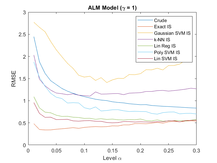
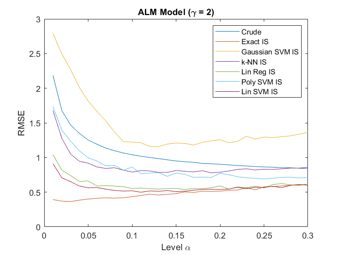
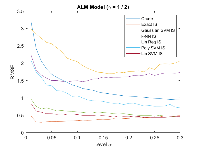
In this section, we apply the developed method to various test models and distributions. The goal is to experimentally evaluate the variance reduction achieved by the proposed algorithm compared to importance sampling in the exact model, which is known in closed form for the test cases. We compare the root mean square errors (RMSEs) when estimating different DRMs induced by concave and convex distortion functions.
3.1 Simulation Design
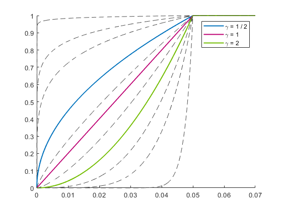
We consider the distortion function with illustrated in Figure 1, see Example A.6 in the Appendix for more details. The concave function defines a convex DRM, is convex, and corresponds to the AV@R at level .
In our numerical experiments, we repeat Algorithm 1 for DRM estimation times to obtain data that can be further analyzed. For clear benchmarking, we specify the hypothesis class used in each of these experiments and compare the results across hypothesis classes. Thus, we do not perform the -fold validation in line 15 of Algorithm 1 in each repetition, but only recalibrate within any previously selected class. Additionally, we identify the winner of a -fold validation with based on pivot samples. Numerical tests in the context of our case studies show that this determination of a ML hypothesis class is quite robust, i.e., different sets of pivot samples typically lead to the selection of the same class.
We consider the following functions and distributions:
-
(1)
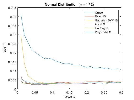
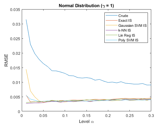
Identity of Normal: We set and , implying . The -fold cross validation from the pivot samples suggests using a linear regression to approximate .
-
(2)
Sum of Normals: We consider with and . The -fold cross validation suggests a linear regression.
-
(3)
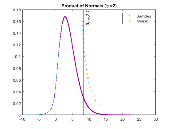
Product of Normals: Let with and . The -fold validation identifies the SVM with a polynomial kernel of degree as the best choice for .
-
(4)
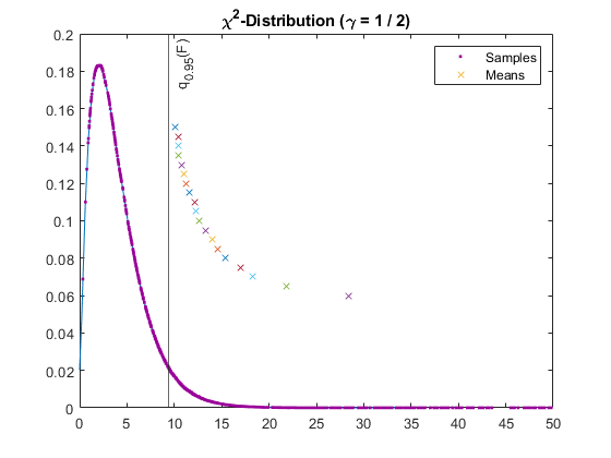
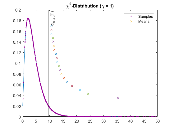
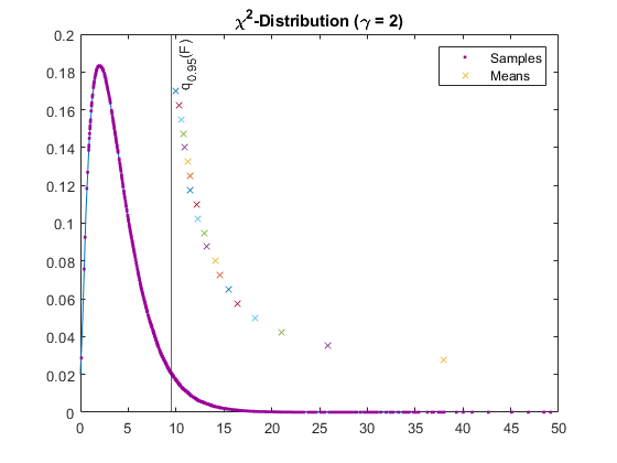
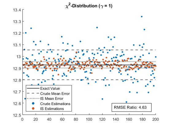
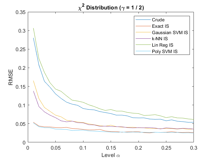
Sum of Squared Normals: Consider the independent random variables and let . Then follows a distribution with degrees of freedom. The -fold validation suggests a polynomial support vector machine with degree .
-
(5)
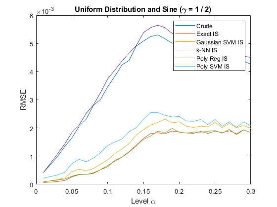
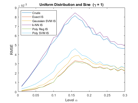
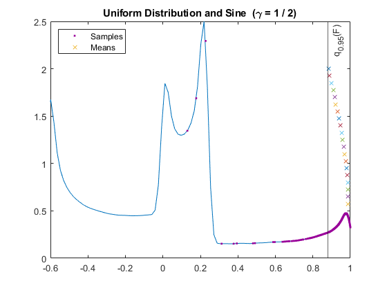
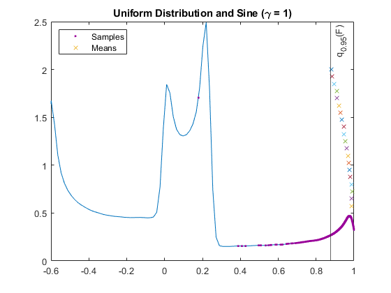
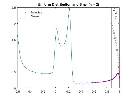
Sine and Uniform: Set and . This example is used in Altman (1992) to illustrate -NN regression. The -fold validation suggests polynomial regression with degree as an approximation of .
-
(6)
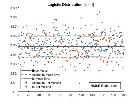
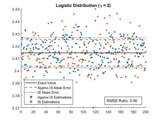
Logistic Transformation and Exponential: Letting , then with follows a distribution. The -fold validation suggests either a support vector machine with Gaussian kernel or -NN regression with .
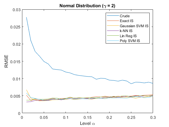
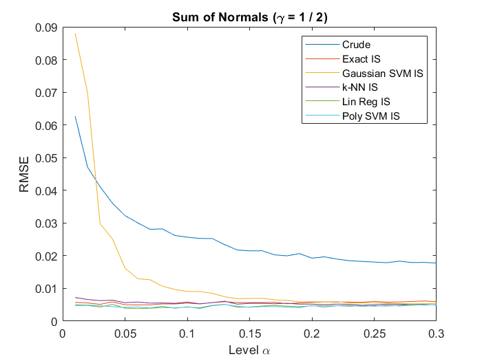
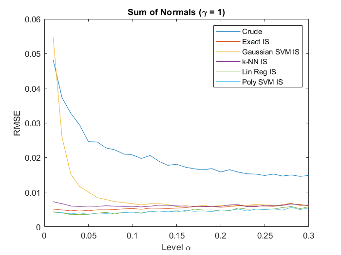
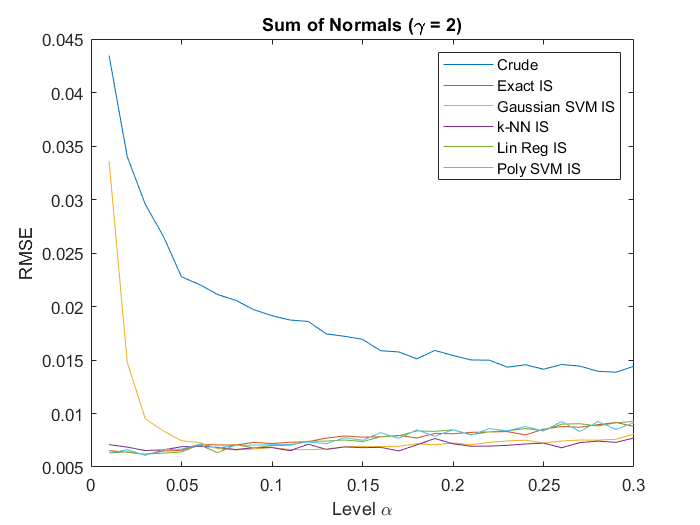
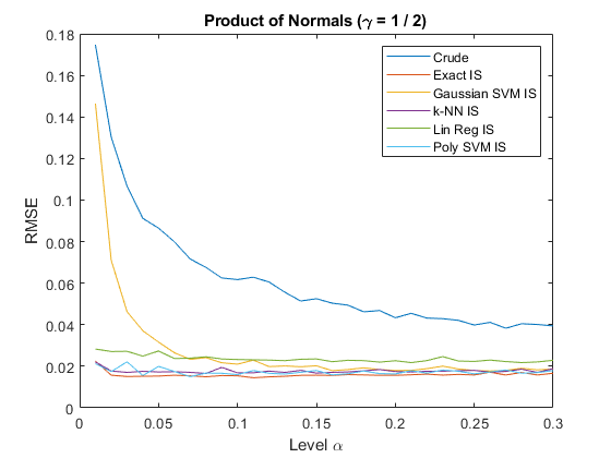
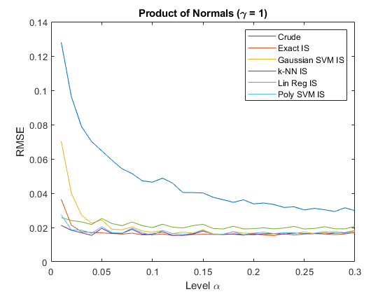
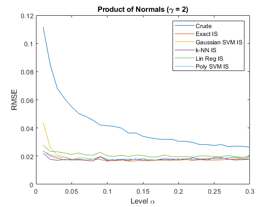
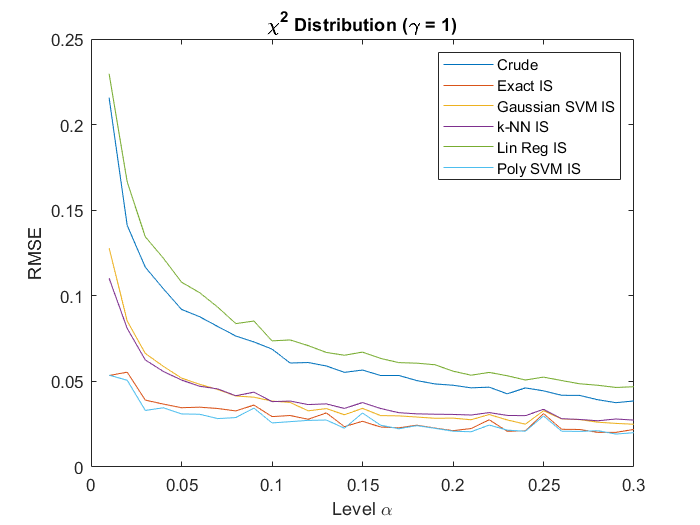
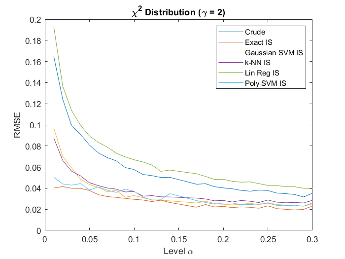
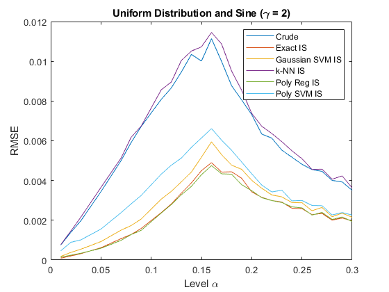
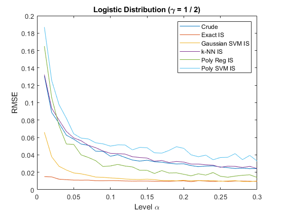
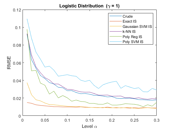
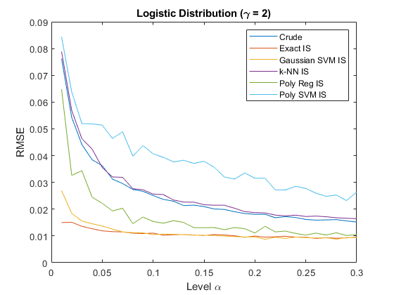
For each of these functions and distributions, we perform numerical experiments for different ML hypothesis classes used to approximate in the importance sampling algorithms. In particular, this analysis is also performed for the winner of the -fold validations. Each experiment is repeated times. In all cases, we implement a crude estimation with samples as well as an estimation based on the importance sampling method with pivot samples and samples from the mixture distribution defined in Section 2.3. As a benchmark, we determine an “exact value” by a crude estimation with samples. From the replications we obtain for all cases an estimated root mean-square error (RMSE).
3.2 Results
3.2.1 Distribution of the Samples
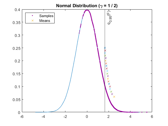
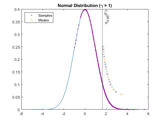
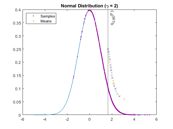
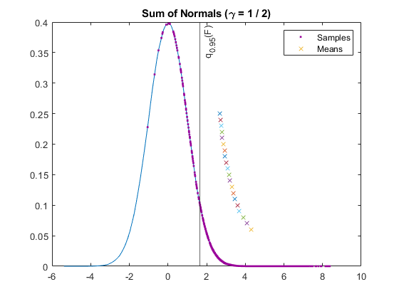
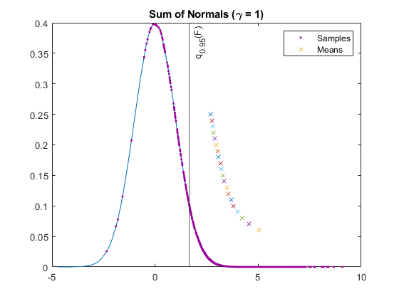
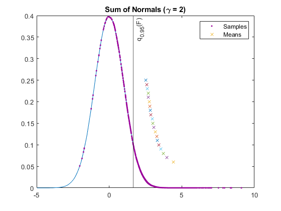
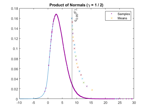
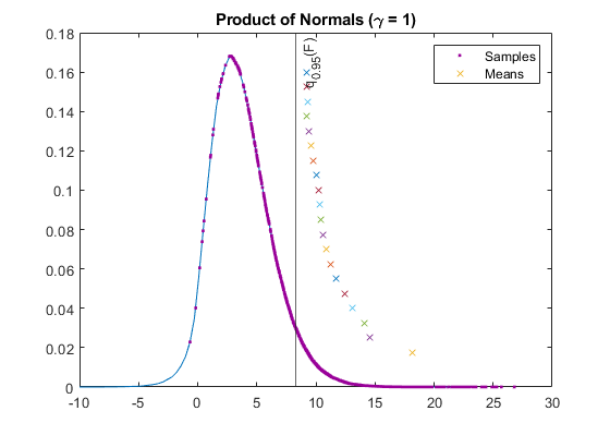
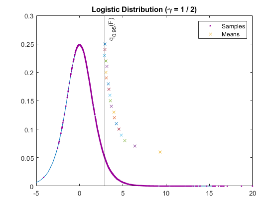
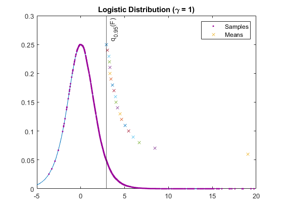
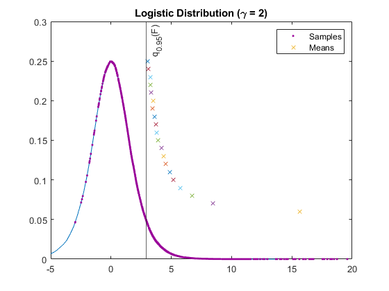
To illustrate the measure change, we consider model (5) in Figure 2. As mentioned before, option 2 in line 23 of Algorithm 1 was implemented in all case studies. An analogous analysis for models (1)-(4) & (6) can be found in Figures 6 & 7. We consider the DRMs , . The figures show the true density of . Additionally, samples from the mixture distribution (with values on the x-axis) are plotted along the probability density. The labeled quantile indicates the threshold above which samples are relevant for the estimation of . The crosses mark the expectations of the individual importance sampling components of the mixture distribution. Samples and expectations are, by construction, in the right tail of the distribution in the area relevant for the estimation of the DRM.
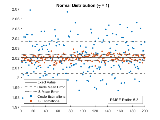
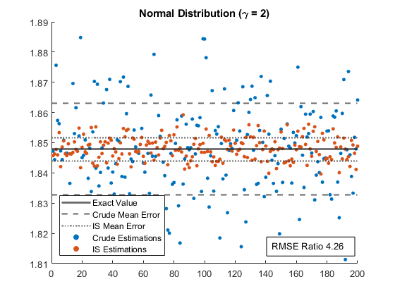
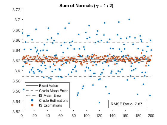
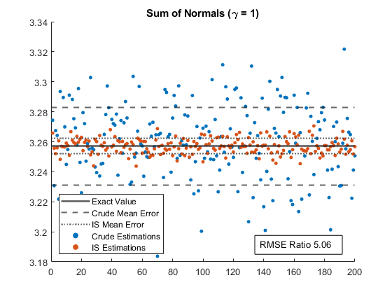
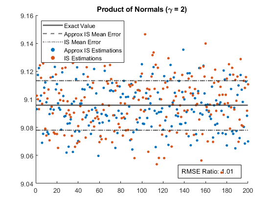
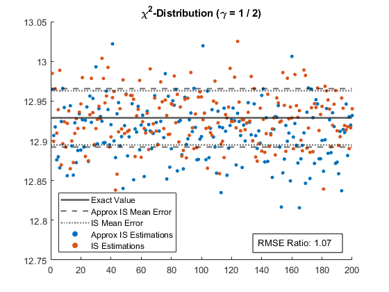
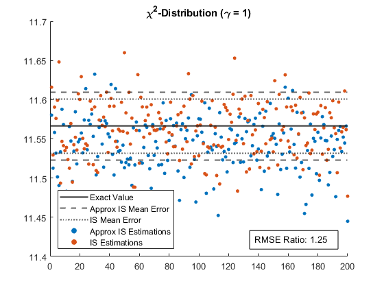
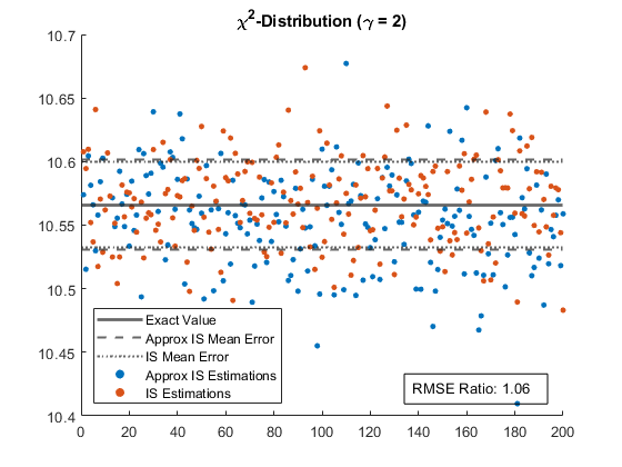
3.2.2 Efficiency of the Estimations
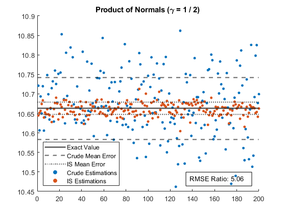
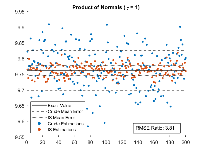
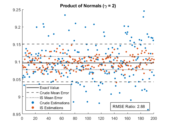
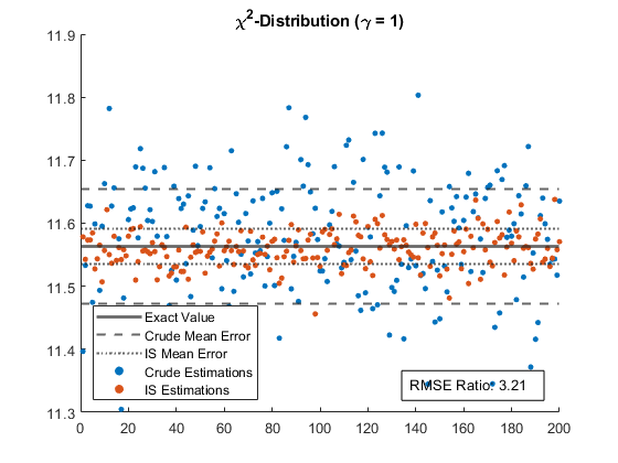
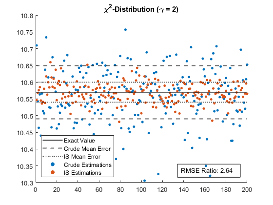
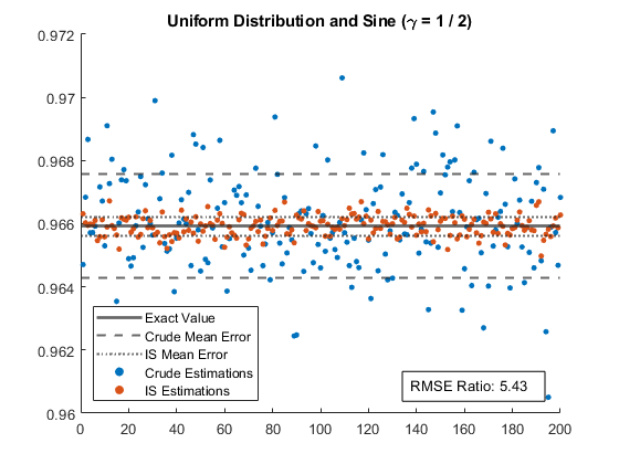
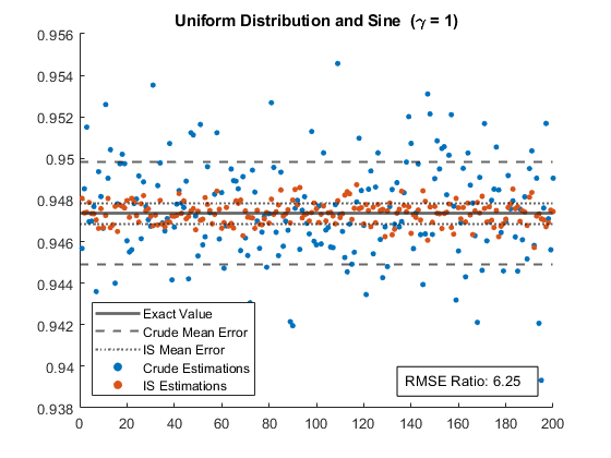
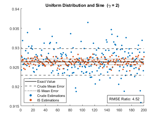
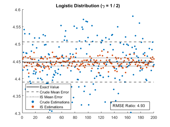
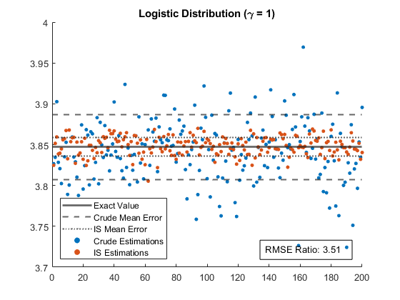
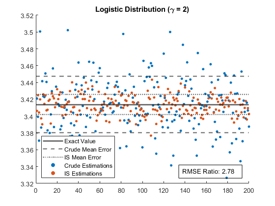
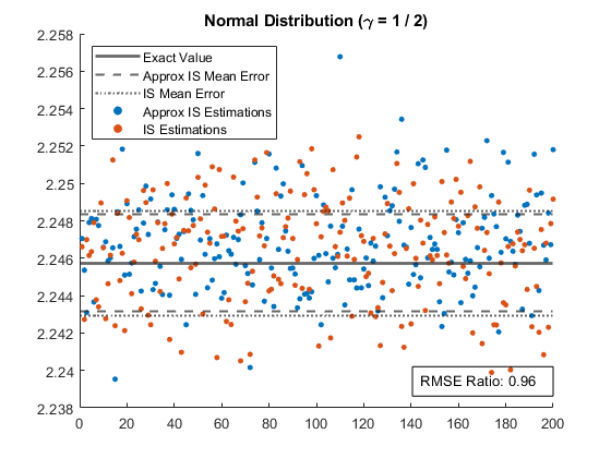
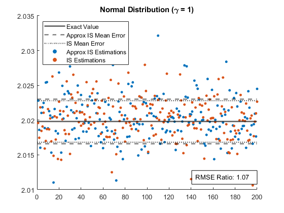
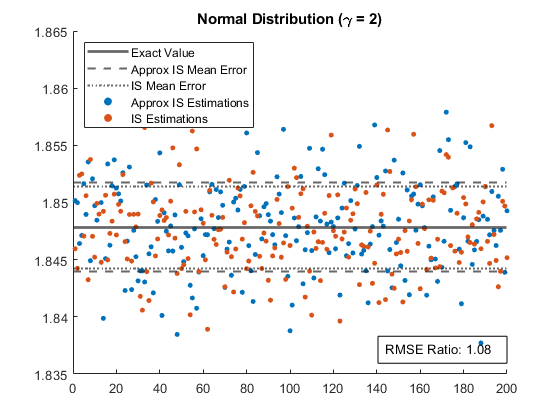
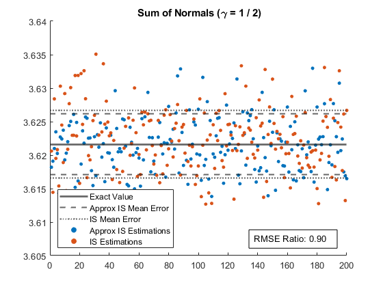
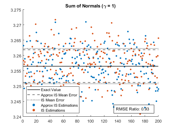
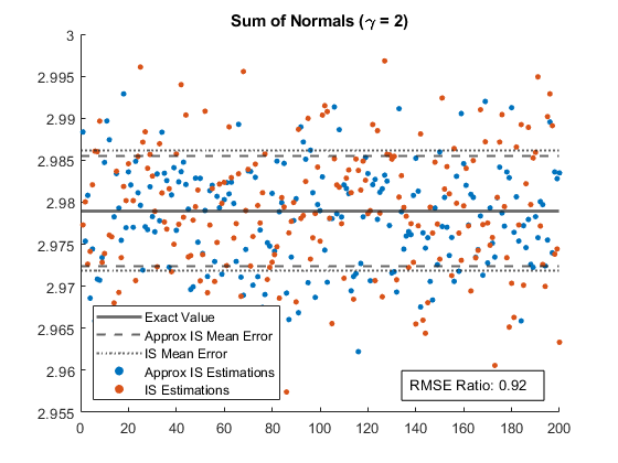
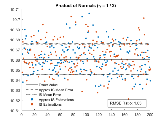
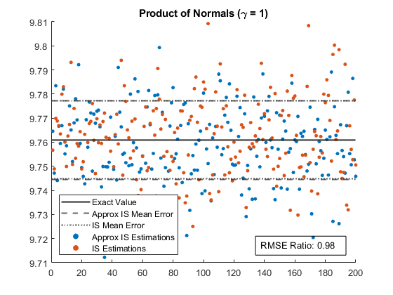
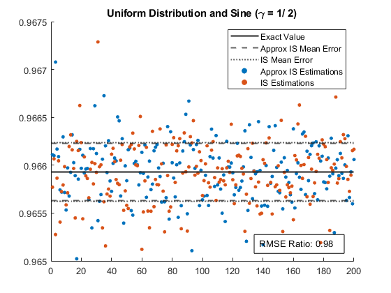
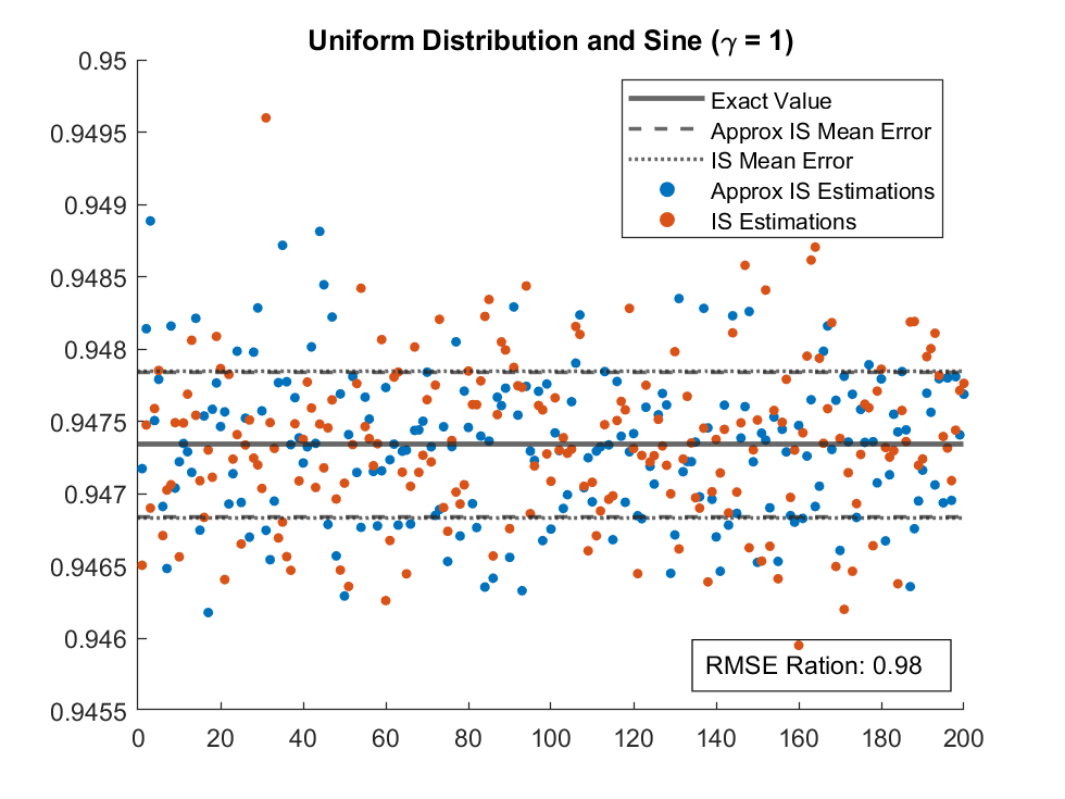
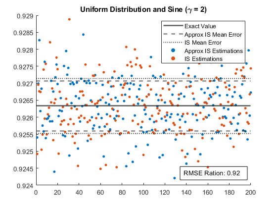
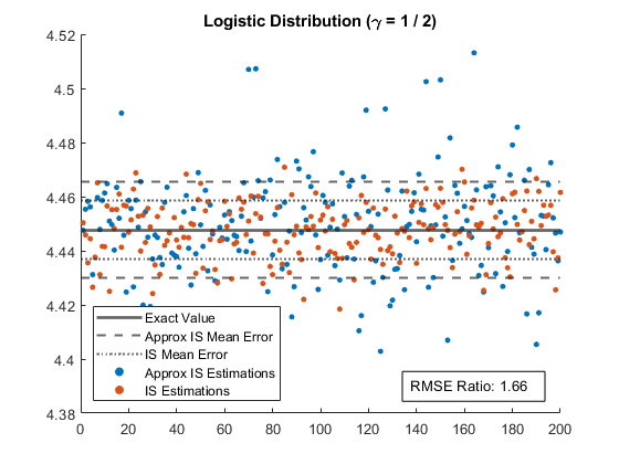
In this section, we discuss the efficiency of the algorithm for case studies (1)-(6). The ML approximation used in importance sampling is fixed, and we compare different hypothesis classes. The calibration of the ML regressions and the construction of the importance sampling measure change are based on pivot samples. We choose and and run replications of the simulation for estimating the RMSE. In Figure 3 & 4, the ratio of the RMSE between the crude estimate and the proposed importance sampling method for the DRMs with and for models (1) to (6). The absolute estimated RMSE for the different estimation methods is shown in Figure 12 & 13 in Appendix A.7.
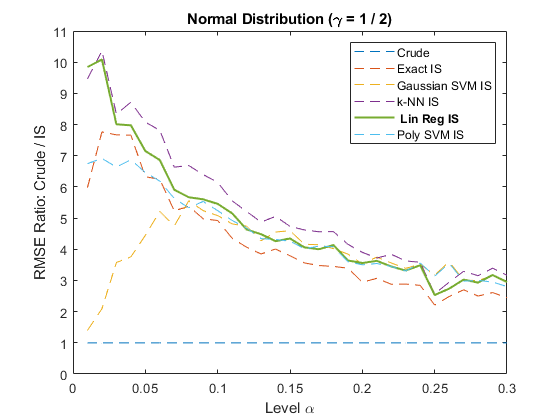
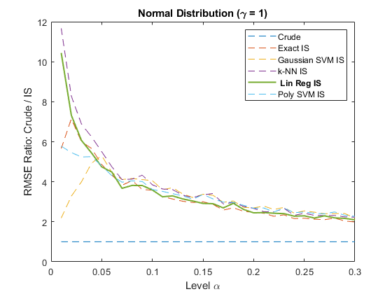
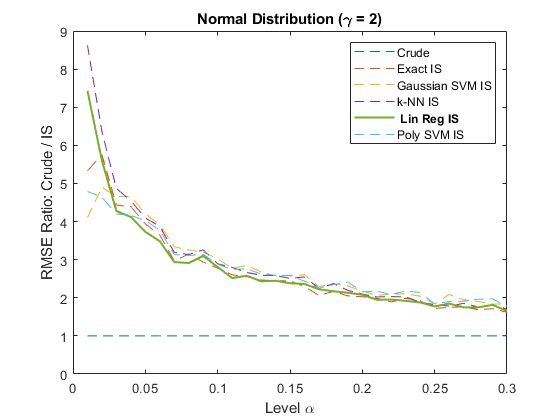
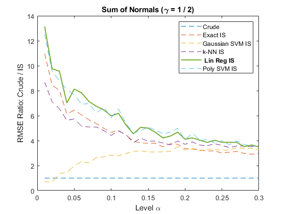
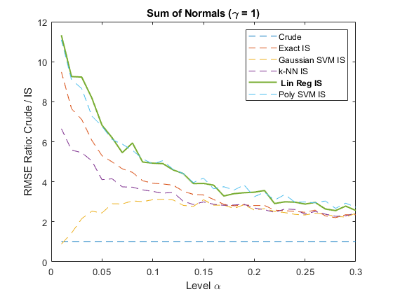
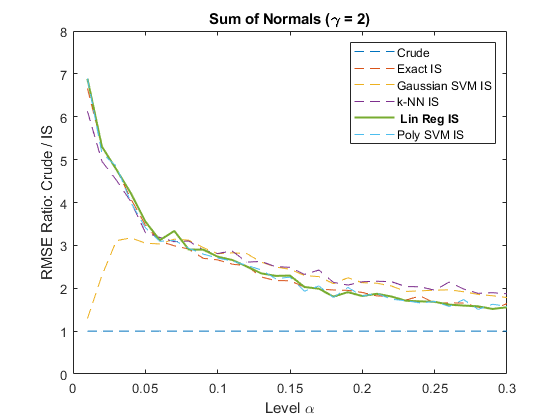
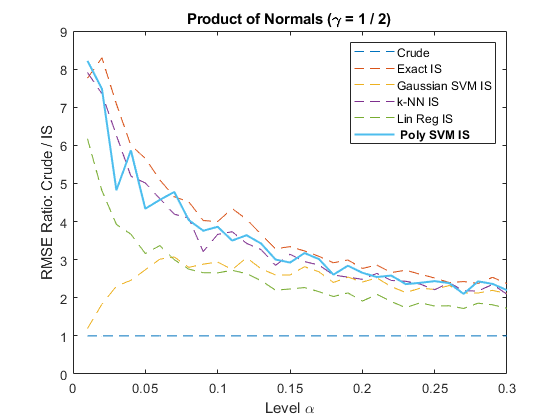
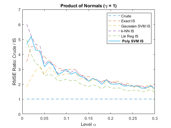
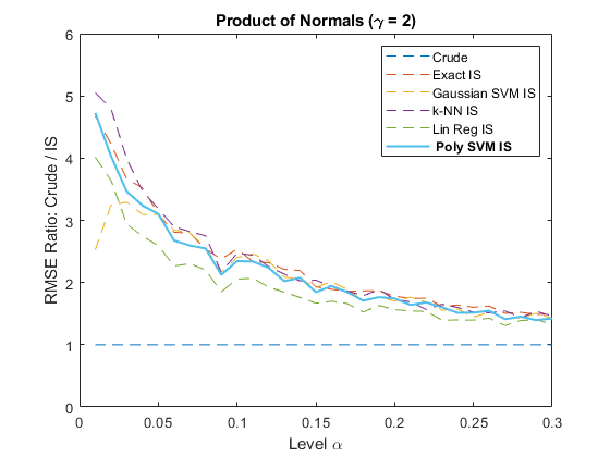
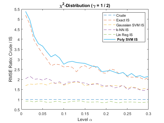
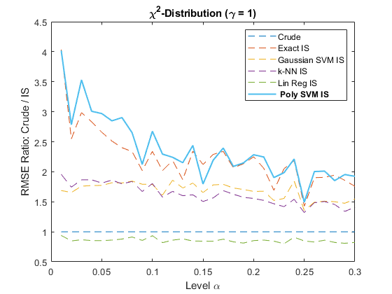
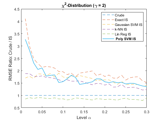
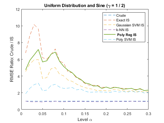
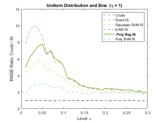
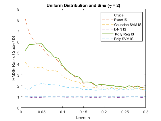
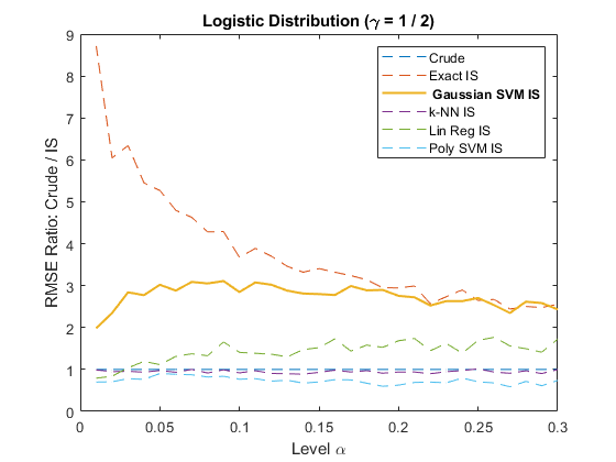
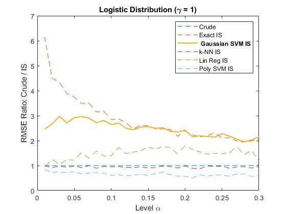
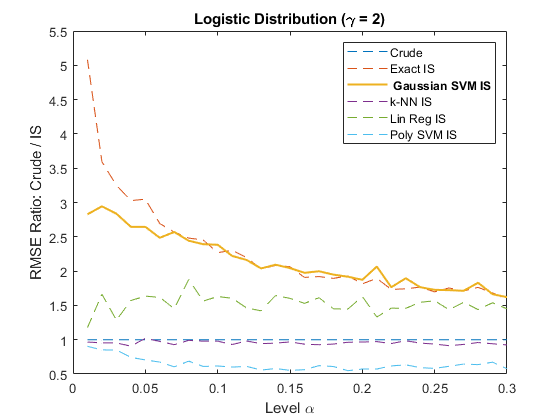
The plots confirm that the proposed importance sampling algorithm can successfully reduce the RMSE in all cases. The efficiency of the algorithm depends strongly on the ML regression chosen. A poorly chosen approximation can even lead to a higher error than the crude method. Interestingly, the choice based on -fold validation and pivot calibration works reasonably well in all cases, despite the fact that the ML objective function does not focus on the tail. The smaller , the more the DRM zooms in on the tail risk due to rare events. As expected, the variance reduction becomes better the smaller is. Similarly, variance reduction is also better the smaller , since DRMs with smaller put more emphasis on tail risk.
3.3 Iterative Exploration of the Extreme Tail
The discussed algorithm consists of two simulation steps. First, pivot samples are drawn that are used for both the choice of the ML approximation and the determination of an IS measure change. Second, samples are generated under the IS distribution and used for the estimation of the DRMs. However, if DRMs are considered that focus on particularly extreme tail events, this approach might not yet be sufficient. A possible extension to the suggested approach is the following: The samples from the IS distribution are not directly used for DRM estimation, but serve as additional data for calibrating the ML approximation a second time and the construction of a further measure change on this basis. In this section, we provide a case study that takes this approach – the iterative exploration of the extreme tail.
Simulation Desgin
We consider again the case studies (1) - (4) outlined in Section 3.1 with the same distortion functions , and corresponding DRMs. We do, however, focus, on more extreme tail events by choosing . In addition, we choose a finer partition by setting . In the experiment, we repeat all simulation runs times to estimate the RMSE. We compare three simulation approaches for the estimation of the DRMs. In all cases, samples are used, respectively.
The first approach is a crude simulation with samples. The second approach is the algorithm suggested in the previous sections with pivot samples and samples from the IS distribution. The third approach is an iterative exploration: pivot samples are used to calculate the IS distribution for level . Then we draw from this IS distribution additional pivot samples. The IS distribution for is computed from the total pivot samples. In the last step, are drawn from this distribution to estimate the DRMs.
Results
| (1) Id. of Normals | (2) Sum of Normals | (3) Prod. of Normals | (4) Sum of Sq. Normals | |||||||||
| Exact | ||||||||||||
| Mean CRUDE | ||||||||||||
| Mean IS | ||||||||||||
| Mean ITER IS | ||||||||||||
| RMSE | ||||||||||||
| RMSE | ||||||||||||
The results of the case study are displayed in Table 1. The exact values of the DRMs, the means over simulation runs and the corresponding ratios of the RMSE of the two IS methods and the crude method are documented. Overall the iterative method generally yields the best RMSE reduction, outperforming the direct IS approach substantially in experiments (2) and (4). The direct IS approach is still more efficient than the crude method. Especially in (1) and (2) the reduction of the RMSE is substantial in contrast to the crude method, while in (3) and (4) the IS methods are not as efficient. When considering the mean over all simulation runs, we observe that the IS methods also reduce estimation bias.
4 Application to ALM
We apply Algorithm 1 to the estimation of solvency capital in a simple asset-liability management (ALM) model of an insurance firm. Instead of the risk measure which forms the basis of Solvency II, we use the same DRMs that we considered in Section 3. The suggested method could also be applied in highly complex ALM models such as those applied by major insurance groups.
4.1 Model Description
Our ALM model, inspired by Weber et al. (2014) and Hamm et al. (2019), describes a snapshot in time of an ongoing insurance business. The focus is on a one-year time horizon with dates , as in Solvency II. The values of assets and liabilities are denoted by , , respectively. At each point in time, their difference is the book value of equity , , which is used for the solvency capital calculation.
The evolution of balance sheet is driven by market and insurance risks. For simplicity, we assume that reserves are constant, i.e., . Any changes in value are thus seen on the asset side. We assume that insurance claims are modeled by a collective model where the number of claims are given by the counting process and their severities by independent, identically distributed losses . Annual total premium payments are received at the beginning of the year. We set
The random annual return of assets between dates and is denoted by , i.e., we obtain that
In order to model the random return of assets we assume that
where and are the prices of a bond and a stock and and the respective holdings. This implies that
where is the fraction of initial wealth invested in the stock. Setting , for some random interest rate , and ,
we derive that
Solvency capital is determined in terms of risk measure applied to the difference of the net asset values over the time period of one year, i.e.,
4.2 Simulation Overview
As in Section 3, we apply the proposed importance sampling method to the DRMs with distortion function and . In terms of the DRMs, solvency capital is . The underlying random factors are . We set and , where is beta distributed with parameters , i.e., . The parameters of the stock are , , , and we assume that half of the available capital is invested into the stock, i.e., . For the collective model, we assume that is a Poisson random variable with parameter , and are independent exponentially distributed random variables with parameter . The premium and reserve are resp. of the expected claims such that and .
As in Section 3, the importance sampling estimates with the different ML approximations used in the measure changes are performed with pivot samples for calibration of the approximation and determination of the importance sampling mixture distribution, and samples of the mixture distribution for DRM estimation. As comparison a crude estimation with samples is implemented. We always use a discretization with . The ‘exact value” of benchmarking is determined with a crude estimation with samples and used to calculate the RMSE over simulation runs.
4.3 Results
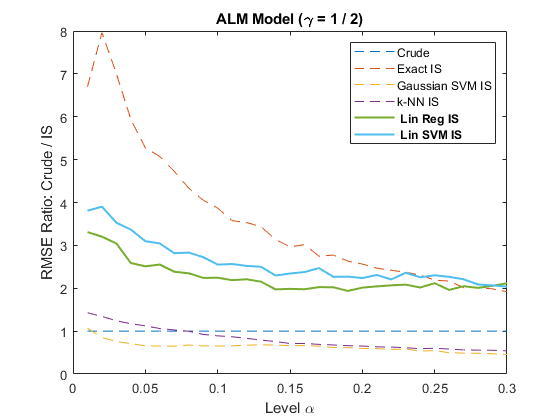
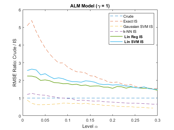
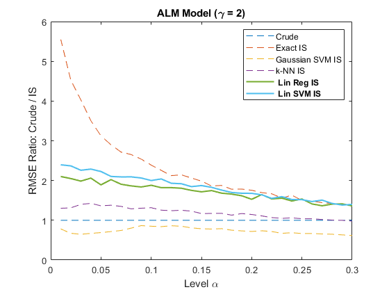
The results of the simulations are shown in Figure 5, which presents the ratio of the RMSEs of the crude method and the studied importance sampling methods. For further reference, the absolute RMSE of the estimates are provided in Figure 14 in Appendix A.7. For all DRMs, importance sampling with exact knowledge of the model leads to a significant reduction in the RMSE, especially for small . The variance reduction decreases for larger . For , the exact method achieves the highest observed RMSE ratio of for . Importance sampling with linear regression leads to a maximum reduction of for . For the DRMs with concave () and convex () distortion functions, the linear SVM gives the best reduction in RMSE. For , the best ratio obtained with full knowledge of the model is for , and with linear SVM, the maximum reduction is for . For , the exact importance sampling method has the best ratio of for and with the linear SVM approximation of for . Across all the different estimated DRMs, we see that the importance sampling methods with Gaussian SVM and -NN regression can lead to a worse RMSE than the crude method. The worst ratio is observed in all cases with the Gaussian SVM with as for , as for and and for with .
In summary, the proposed method provides a good path to variance reduction. However, the ML approximation in the measure change needs to be chosen carefully, but -fold validation seems to work quite well. The variance reduction becomes better the more the risk measure depends on extreme tail events. In the ALM case study, the most extreme parameter was . We expect that the iterative procedure outlined in Section 3.3 would also lead to further improvements in variance reduction when the very extreme tail is considered.
References
- Acerbi (2002) Carlo Acerbi. Spectral measures of risk: A coherent representation of subjective risk aversion. Journal of Banking & Finance, 26(7):1505–1518, 2002.
- Ahn and Shyamalkumar (2011) Jae Youn Ahn and Nariankadu D. Shyamalkumar. Large sample behavior of the CTE and VaR estimators under importance sampling. North American Actuarial Journal, 15(3):393–416, 2011. doi: 10.1080/10920277.2011.10597627.
- Altman (1992) Naomi S. Altman. An introduction to kernel and nearest-neighbor nonparametric regression. The American Statistician, 46(3):175, 1992. doi: 10.2307/2685209.
- Arief et al. (2021) Mansur Arief, Yuanlu Bai, Wenhao Ding, Shengyi He, Zhiyuan Huang, Henry Lam, and Ding Zhao. Certifiable deep importance sampling for rare-event simulation of black-box systems, 2021.
- Artzner et al. (1999) Philippe Artzner, Freddy Delbaen, Jean-Marc Eber, and David Heath. Coherent measures of risk. Mathematical Finance, 9(3):203–228, 1999. doi: 10.1111/1467-9965.00068.
- Asmussen et al. (2000) Søren Asmussen, Klemens Binswanger, and Bjarne Højgaard. Rare events simulation for heavy-tailed distributions. Bernoulli, 6(2):303, 2000. doi: 10.2307/3318578.
- Asmussen and Glynn (2007) Søren Asmussen and Peter W. Glynn. Stochastic Simulation: Algorithms and Analysis, volume 57. Springer, 2007.
- Bannör and Scherer (2014) Karl F. Bannör and Matthias Scherer. On the calibration of distortion risk measures to bid-ask prices. Quantitative Finance, 14(7):1217–1228, 2014.
- Ben-Tal and Teboulle (2007) Aharon Ben-Tal and Marc Teboulle. An old-new concept of convex risk measures: the optimized certainty equivalent. Mathematical Finance, 17(3):449–476, 2007.
- Bettels et al. (2022) Sören Bettels, Sojung Kim, and Stefan Weber. Multinomial backtesting of distortion risk measures, 2022.
- Beutner and Zähle (2010) Eric Beutner and Henryk Zähle. A modified functional delta method and its application to the estimation of risk functionals. Journal of Multivariate Analysis, 101(10):2452–2463, 2010. doi: 10.1016/j.jmva.2010.06.015.
- Bignozzi and Tsanakas (2015) Valeria Bignozzi and Andreas Tsanakas. Parameter uncertainty and residual estimation risk. Journal of Risk and Insurance, 83(4):949–978, 2015. doi: 10.1111/jori.12075.
- Blanchet and Glynn (2008) Jose Blanchet and Peter Glynn. Efficient rare-event simulation for the maximum of heavy-tailed random walks. The Annals of Applied Probability, 18(4), 2008. doi: 10.1214/07-aap485.
- Brazauskas et al. (2008) Vytaras Brazauskas, Bruce L. Jones, Madan L. Puri, and Ričardas Zitikis. Estimating conditional tail expectation with actuarial applications in view. Journal of Statistical Planning and Inference, 138(11):3590–3604, 2008. doi: 10.1016/j.jspi.2005.11.011.
- Bucklew (2004) James Antonio Bucklew. Introduction to Rare Event Simulation. Springer New York, 2004.
- Cherny and Madan (2008) Alexander Cherny and Dilip Madan. New measures for performance evaluation. Review of Financial Studies, 22(7):2571–2606, 2008. doi: 10.1093/rfs/hhn081.
- Choquet (1954) Gustave Choquet. Theory of capacities. Annales de l’institut Fourier, 5:131–295, 1954. doi: 10.5802/aif.53.
- Denneberg (1994) Dieter Denneberg. Non-Additive Measure and Integral. Springer Netherlands, 1994. doi: 10.1007/978-94-017-2434-0.
- Dhaene et al. (2006) Jan Dhaene, Steven Vanduffel, Marc J. Goovaerts, Rob Kaas, Qihe Tang, and David Vyncke. Risk measures and comonotonicity: A review. Stochastic Models, 22(4):573–606, 2006. doi: 10.1080/15326340600878016.
- Dhaene et al. (2012) Jan Dhaene, Alexander Kukush, Daniël Linders, and Qihe Tang. Remarks on quantiles and distortion risk measures. European Actuarial Journal, 2(2):319–328, 2012. doi: 10.1007/s13385-012-0058-0.
- Dowd et al. (2008) Kevin Dowd, John Cotter, and Ghulam Sorwar. Spectral risk measures: Properties and limitations. Journal of Financial Services Research, 34(1):61–75, 2008. doi: 10.1007/s10693-008-0035-6.
- Drucker et al. (1996) Harris Drucker, Christopher J. Burges, Linda Kaufman, Alex Smola, and Vladimir Vapnik. Support vector regression machines. Advances in Neural Information Processing Systems, 9, 1996.
- Dunkel and Weber (2007) Jørn Dunkel and Stefan Weber. Efficient monte carlo methods for convex risk measures in portfolio credit risk models. In 2007 Winter Simulation Conference. IEEE, 2007. doi: 10.1109/wsc.2007.4419692.
- Dupuis and Wang (2002) Paul Dupuis and Hui Wang. Importance sampling, large deviations, and differential games. Technical report, 2002.
- El Methni and Stupfler (2017) Jonathan El Methni and Gilles Stupfler. Extreme versions of wang risk measures and their estimation for heavy-tailed distributions. Statistica Sinica, pages 907–930, 2017.
- Fan et al. (2005) Rong-En Fan, Pai-Hsuen Chen, Chih-Jen Lin, and Thorsten Joachims. Working set selection using second order information for training support vector machines. Journal of Machine Learning Research, 6(12), 2005.
- Folland (1999) Gerald B. Folland. Real Analysis: Modern Techniques and Their Applications. Wiley, 1999. ISBN 0471317160.
- Frittelli and Gianin (2002) Marco Frittelli and Emanuela Rosazza Gianin. Putting order in risk measures. Journal of Banking & Finance, 26(7):1473–1486, 2002. doi: 10.1016/s0378-4266(02)00270-4.
- Föllmer and Schied (2002) Hans Föllmer and Alexander Schied. Convex measures of risk and trading constraints. Finance and Stochastics, 6(4):429–447, 2002.
- Föllmer and Schied (2016) Hans Föllmer and Alexander Schied. Stochastic Finance. De Gruyter, 2016. doi: 10.1515/9783110463453.
- Föllmer and Weber (2015) Hans Föllmer and Stefan Weber. The axiomatic approach to risk measures for capital determination. Annual Review of Financial Economics, 7(1):301–337, 2015. doi: 10.1146/annurev-financial-111914-042031.
- Glasserman (2003) Paul Glasserman. Monte Carlo Methods in Financial Engineering. Springer New York, 2003.
- Glasserman et al. (2002) Paul Glasserman, Philip Heidelberger, and Perwez Shahabuddin. Portfolio value-at-risk with heavy-tailed risk factors. Mathematical Finance, 12(3):239–269, 2002. doi: 10.1111/1467-9965.00141.
- Glynn (1996) Peter W. Glynn. Importance sampling for monte carlo estimation of quantiles. In Mathematical Methods in Stochastic Simulation and Experimental Design: Proceedings of the 2nd St. Petersburg Workshop on Simulation, pages 180–185. Citeseer, 1996.
- Guégan and Hassani (2014) Dominique Guégan and Bertrand Hassani. Distortion risk measure or the transformation of unimodal distributions into multimodal functions. In Future Perspectives in Risk Models and Finance, pages 71–88. Springer International Publishing, 2014.
- Guillen et al. (2018) Montserrat Guillen, Jose Maria Sarabia, Jaume Belles-Sampera, and Faustino Prieto. Distortion risk measures for nonnegative multivariate risks. Journal of Operational Risk, 13(2):35–57, 2018. doi: 10.21314/jop.2018.206.
- Hamm et al. (2019) Anna-Maria Hamm, Thomas Knispel, and Stefan Weber. Optimal risk sharing in insurance networks. European Actuarial Journal, 10(1):203–234, 2019.
- Huang et al. (2020) Jian Huang, Junyi Chai, and Stella Cho. Deep learning in finance and banking: A literature review and classification. Frontiers of Business Research in China, 14(1):1–24, 2020.
- Huang et al. (2006) Te-Ming Huang, Vojislav Kecman, and Ivica Kopriva. Kernel Based Algorithms for Mining Huge Data Sets, volume 1. Springer, 2006.
- Hult and Nyquist (2016) Henrik Hult and Pierre Nyquist. Large deviations for weighted empirical measures arising in importance sampling. Stochastic Processes and their Applications, 126(1):138–170, 2016. doi: 10.1016/j.spa.2015.08.002.
- Juneja and Shahabuddin (2006) Sandeep Juneja and Perwez Shahabuddin. Chapter 11 rare-event simulation techniques: An introduction and recent advances. In Simulation, pages 291–350. Elsevier, 2006. doi: 10.1016/s0927-0507(06)13011-x.
- Kim and Weber (2022) Sojung Kim and Stefan Weber. Simulation methods for robust risk assessment and the distorted mix approach. European Journal of Operational Research, 298(1):380–398, 2022. doi: 10.1016/j.ejor.2021.07.005.
- Kusuoka (2001) Shigeo Kusuoka. On law invariant coherent risk measures. In Advances in Mathematical Economics, pages 83–95. Springer Japan, 2001.
- Li et al. (2018) Lujun Li, Hui Shao, Ruodu Wang, and Jingping Yang. Worst-case range value-at-risk with partial information. SIAM Journal on Financial Mathematics, 9(1):190–218, 2018. doi: 10.1137/17m1126138.
- Mohri et al. (2018) Mehryar Mohri, Afshin Rostamizadeh, and Ameet Talwalkar. Foundations of Machine Learning. MIT Press, 2018.
- Pandey et al. (2021) Ajay Kumar Pandey, L.A. Prashanth, and Sanjay P. Bhat. Estimation of spectral risk measures. Proceedings of the AAAI Conference on Artificial Intelligence, 35(13):12166–12173, 2021. doi: 10.1609/aaai.v35i13.17444.
- Platt (1998) John Platt. Sequential minimal optimization: A fast algorithm for training support vector machines. 1998.
- Rockafellar and Uryasev (2000) R. Tyrrell Rockafellar and Stanislav Uryasev. Optimization of conditional value-at-risk. Journal of Risk, 2(3):21–41, 2000.
- Rockafellar and Uryasev (2002) R. Tyrrell Rockafellar and Stanislav Uryasev. Conditional value-at-risk for general loss distributions. Journal of Banking Finance, 26:1443–1471, 2002.
- Rosenblatt (1958) Frank Rosenblatt. The perceptron: A probabilistic model for information storage and organization in the brain. Psychological Review, 65(6):386–408, 1958.
- Rubino and Tuffin (2009) Gerardo Rubino and Bruno Tuffin. Rare Event Simulation using Monte Carlo Methods. Wiley, 2009. ISBN 9780470772690.
- Samanthi and Sepanski (2018) Ranadeera G.M. Samanthi and Jungsywan Sepanski. Methods for generating coherent distortion risk measures. Annals of Actuarial Science, 13(2):400–416, 2018. doi: 10.1017/s1748499518000258.
- Serfling (1980) Robert J. Serfling, editor. Approximation Theorems of Mathematical Statistics. John Wiley & Sons, Inc., 1980. doi: 10.1002/9780470316481.
- Shalev-Shwartz and Ben-David (2014) Shai Shalev-Shwartz and Shai Ben-David. Understanding Machine Learning: From Theory to Algorithms. Cambridge University Press, 2014.
- Shampine (2008) Lawrence F. Shampine. Matlab program for quadrature in 2d. Applied Mathematics and Computation, 202(1):266–274, 2008.
- Smola and Schölkopf (2004) Alex J. Smola and Bernhard Schölkopf. A tutorial on support vector regression. Statistics and Computing, 14(3):199–222, 2004. doi: 10.1023/B:STCO.0000035301.49549.88.
- Song and Yan (2009a) Yongsheng Song and Jia-An Yan. Risk measures with comonotonic subadditivity or convexity and respecting stochastic orders. Insurance: Mathematics and Economics, 45(3):459–465, 2009a. doi: 10.1016/j.insmatheco.2009.09.011.
- Song and Yan (2006) Yongsheng Song and Jia’an Yan. The representation of two types functionals on and . Science in China Series A: Mathematics, 49(10):1376–1382, 2006. doi: 10.1007/s11425-006-2010-8.
- Song and Yan (2009b) YongSheng Song and JiaAn Yan. An overview of representation theorems for static risk measures. Science in China Series A: Mathematics, 52(7):1412–1422, 2009b. doi: 10.1007/s11425-009-0122-7.
- Stigler (1974) Stephen M. Stigler. Linear functions of order statistics with smooth weight functions. The Annals of Statistics, 2(4), 1974. doi: 10.1214/aos/1176342756.
- Sun and Hong (2009) Lihua Sun and L. Jeff Hong. A general framework of importance sampling for value-at-risk and conditional value-at-risk. In Proceedings of the 2009 Winter Simulation Conference (WSC), pages 415–422. IEEE, 2009.
- Vapnik (1999) Vladimir Vapnik. The Nature of Statistical Learning Theory. Springer Science & Business Media, 1999.
- Wang (1995) Shaun Wang. Insurance pricing and increased limits ratemaking by proportional hazards transforms. Insurance: Mathematics and Economics, 17(1):43–54, 1995. doi: 10.1016/0167-6687(95)00010-p.
- Wang (1996) Shaun Wang. Premium calculation by transforming the layer premium density. ASTIN Bulletin: The Journal of the IAA, 26(1):71–92, 1996.
- Wang (2000) Shaun S Wang. A class of distortion operators for pricing financial and insurance risks. Journal of Risk and Insurance, pages 15–36, 2000.
- Wang (2001) Shaun S. Wang. A risk measure that goes beyond coherence. 2001.
- Weber (2018) Stefan Weber. Solvency II, or how to sweep the downside risk under the carpet. Insurance: Mathematics and Economics, 82:191–200, 2018. doi: 10.1016/j.insmatheco.2017.11.010.
- Weber et al. (2014) Stefan Weber, Anna-Maria Hamm, Torsten Becker, Claudia Cottin, Matthias Fahrenwaldt, and Stefan Nörtemann. Market consistent embedded value – eine praxisorientierte Einführung. Der Aktuar, 1:4–8, 2014.
- Wirch and Hardy (1999) Julia Lynn Wirch and Mary R. Hardy. A synthesis of risk measures for capital adequacy. Insurance: Mathematics and Economics, 25(3):337–347, 1999. doi: 10.1016/s0167-6687(99)00036-0.
- Wozabal (2014) David Wozabal. Robustifying convex risk measures for linear portfolios: A nonparametric approach. Operations Research, 62(6):1302–1315, 2014.
- Yitzhaki (1982) Shlomo Yitzhaki. Stochastic dominance, mean variance, and gini’s mean difference. The American Economic Review, 72(1):178–185, 1982.
Appendix A Online Appendix
This is an online appendix that is provided as an electronic supplement to the paper.
A.1 Distortion Risk Measures
We review some facts related to risk measures and the special case of DRMs.
Let denote the set of all bounded and measurable functions on the measurable space
. Elements in model financial positions or insurance losses.
We use the sign convention to interpret positive values as losses and negative values as gains.
The axiomatic definition of risk measures goes back to Artzner et al. (1999); the notion of
distortion risk measures (DRM) was developed by Wang (1996) and Acerbi (2002).
DRMs are a subclass of comonotonic risk measures. The link of comontonic risk measures and
DRMs is briefly discussed in Appendix A.2.
For an excellent overview on risk measures and DRMs we refer
to Föllmer and Schied (2016).
A risk measure is a functional that quantifies the risk of elements of :
Definition A.1.
A mapping is called monetary risk measure if the following properties hold:
-
(i)
Monotonicity: If , , then .
-
(ii)
Cash-Invariance: If and , then .
Risk measures may exhibit additional properties such as quasi-convexity, which in economic terms means that diversification of positions does not increase the measurements. This property can be shown to be equivalent to convexity:
Definition A.2.
A risk measure is called convex, if for ,
A DRM is defined as follows:
Definition A.3.
-
(i)
A non decreasing function with and is called distortion function.
-
(ii)
Let be a probability measure on and be a distortion function. The monetary risk measure defined by
is called a DRM with respect to .
If the distortion function is concave we obtain a convex risk measure (see Föllmer and Schied (2016)):
Theorem A.4.
Consider the distortion function and the corresponding DRM . If is concave, then the DRM is a convex risk measure. If the underlying probability space is atomless, the converse implication is also true.
DRMs can be expressed as mixture of quantiles. One must focus on the details of the continuity properties of the distortion function to obtain the correct representation, as shown in Dhaene et al. (2012).
Theorem A.5.
-
(i)
Let be a right continuous distortion function. Then the DRM is given by
where .
-
(ii)
Let be a left continuous distortion function. Then the DRM is given by
where and , .
Many important risk measures fall into the class of DRMs; for examples see Cherny and Madan (2008), Föllmer and Schied (2016), Weber (2018), and the Appendix A.3. Particularly important examples will be discussed here:
Example A.6.
-
(i)
Let , then is the Value at Risk at level , so that
-
(ii)
The distortion function yields the Average Value at Risk at level , i.e.,
-
(iii)
The distortion function with and generalizes the distortion function of the AV@R () and other special cases such as the hazard transform (, ) and MAXV@R ().
If , the distortion function is concave such that the corresponding DRM is convex. If the distortion function is convex. In this case, the resulting DRM is not convex.
Remark A.7.
Every distortion function can be decomposed in the convex combination of a left and right continuous distortion function (see Dhaene et al. (2012)), such that with and . As a consequence, any distortion risk measure with general distortion function can be expressed as convex combination . The decompositions of and is not unique, unless is a step function. Bettels et al. (2022) point out that a decomposition of into a left and a right continuous step function and a continuous function is unique.
A.2 Comonotonic Risk Measures
We review the links between comonotonic risk measures, Choquet integrals and DRMs. More details can be found in Föllmer and Schied (2016). is a measurable space on which the financial positions in are defined.
Definition A.8.
-
(i)
Two measurable functions on are called comonotonic if
-
(ii)
A risk measure is called comonotonic if
for comonotonic .
Comonotonic risk measures can be expressed as Choquet integrals with respect to capacities.
Definition A.9.
-
(i)
A map is called monotone set function if it satisfies the following properties:
-
a)
.
-
b)
, .
If, in addition, , i.e., is normalized, then is called a capacity.
-
a)
-
(ii)
For the Choquet integral of with respect to the monotone set function is defined by
The Choquet integral coincides with the Lebesgue integral if is a -additive probability measure. The following characterization theorem can, for example, be found in Chapter 4 of Föllmer and Schied (2016).
Theorem A.10.
A monetary risk measure is comonotonic, if and only if there exists a capacity on such that
DRMs are an important special case of the comonotonic risk measures. In this case, the capacity is defined in terms of a distorted probability measure . The resulting capacity is absolutely continuous with respect to , but typically not additive.
Definition A.11.
-
(i)
If is a probability measure on and is a distortion function, then
is called a distorted probability.
-
(ii)
A comonotonic risk measure is called a DRM, if the capacity can be expressed as a distorted probability.
| Name | Distortion | Closed form | Reference |
|---|---|---|---|
| Cherny and Madan (2008) | |||
| Föllmer and Schied (2016) | |||
| Bannör and Scherer (2014) | |||
| Cherny and Madan (2008) | |||
| such that | Föllmer and Schied (2016) | ||
| Bannör and Scherer (2014) | |||
| Cherny and Madan (2008) | |||
| such that | Föllmer and Schied (2016) | ||
| Bannör and Scherer (2014) | |||
| Cherny and Madan (2008) | |||
| such that | Föllmer and Schied (2016) | ||
| Bannör and Scherer (2014) | |||
| Bignozzi and Tsanakas (2015) | |||
| (Range ) | Weber (2018), Li et al. (2018) | ||
| Proportional | Wang (1995, 1996) | ||
| hazard transform | if a.s. | Guillen et al. (2018) | |
| Dual power | , | Wirch and Hardy (1999) | |
| transform | if a.s. | Guillen et al. (2018) | |
| Gini’s principle | Yitzhaki (1982),Wozabal (2014) | ||
| Guillen et al. (2018) | |||
| Exponential | if | - | El Methni and Stupfler (2017) |
| transform | if | Dowd et al. (2008) | |
| Inverse S-shaped | Guégan and Hassani (2014) | ||
| polynomial | - | El Methni and Stupfler (2017) | |
| of degree 3 | |||
| Beta family | - | Samanthi and Sepanski (2018) | |
| Wirch and Hardy (1999) | |||
| Wang transform | - | Wang (2000, 2001) | |
| Wozabal (2014) |
A.3 Examples of DRMs
A.4 Asymptotics of Quantile Estimators in Importance Sampling
The importance sampling estimator in Section 2.1, eq. (2) is studied, along with other alternatives, in Glynn (1996). Obviously, we can equivalently rewrite the estimator in (2) as . Setting , the estimator coincides with the crude Monte Carlo estimator of quantiles, the empirical quantile. We want to analyze under which conditions the estimator in eq. (2) is finite.
For this purpose, we first analyse a deterministic problem. Let , for and . Then
To see this, we denote the inf-term on the left hand side by and observe that is equivalent to for all which simply means that . This would already prove the claim, if was impossible. But the latter equality is equivalent to for all ; for large enough , the sum is empty and equal to , contradicting .
The simple characterization implies for that
| (7) |
If we assume that are independent, identically distributed samples from , then by a law of large numbers , thus eq. (7) is satisfied for large enough.
The asymptotic normality of the estimator can be shown, if the following assumptions holds. This is stated in Theorem 2.1 of Ahn and Shyamalkumar (2011), generalizing Glynn (1996).
Assumption A.12.
Let , be the distribution functions of under , , such that ,
.
Assume that for the following properties hold:
-
(A1)
is absolutely continuous with respect to .
-
(A2)
is continuous at .
-
(A3)
has a strictly positive first derivative at .
-
(A4)
is a function of finite variation on compacts and has finite negative variation on for all .
-
(A5)
is right continuous.
-
(A6)
There exists a such that
Remark A.13.
These assumptions of Ahn and Shyamalkumar (2011) are weaker than the assumptions of Glynn (1996) to obtain the implications in Theorem 2.1. Glynn (1996) assumes that (A1) to (A3) hold and . The latter is replaced by assumption (A6), together with the technical conditions (A4) and (A5); here, denotes total variation.111If is a function of bounded variation, there exist two increasing functions with , and . The former is called the Jordan decomposition of and is closely related to the Hahn decomposition of signed measures. For details we refer to Folland (1999). Ahn and Shyamalkumar (2011) show that if holds for some , then (A6) is satisfied for .
Proposition A.14.
If Assumption A.12 holds, we obtain for :
-
(i)
-
(ii)
Suppose that and are equivalent. Then
Proof.
-
(i)
By assumption is continuous at , such that . The inequality is thus a simple consequence of Jensen’s inequality.
-
(ii)
The function is convex function on . Hence, by Jensen’s inequality we have
∎
We now consider the estimation of the quantile , , by , the estimator defined in Section 2.1, eq. (2). According to Theorem 2.1 we should choose such that
| (8) |
is small. We consider exponential twists given in eq. (3). The following standard result for the cumulant generating function is useful:
Lemma A.15.
Letting be the distribution function of , a measurable function. If for all in some neighborhood of , then where is the family of distributions defined in (3).
To find an appropriate parameter to make (8) small, we take an approach like in Sun and Hong (2009). By the definition of samples in the right tail are more likely to occur when , which also indicates that to minimize (8) we should choose . We observe that
Minimizing the upper bound is then equivalent to minimizing , from which we obtain a first order condition using Lemma A.15
| (9) |
In their paper, Sun and Hong (2009) show that this approach yields a strict reduction of the objective function (8):
Theorem A.16.
Consider the situation as described above. Assume there exists such that is differentiable with strictly positive derivative on . Further suppose that , , and be chosen such that . Then
A.5 Tools from Machine Learning
For convenience, we breifly review the considered ML regression techniques and the methodology of -fold validation. A good introduction to machine learning is Shalev-Shwartz and Ben-David (2014)). In our simulation algorithm, pivot samples are used as training data.
A.5.1 Linear Predictors
We briefly review linear prediction; this is based on Section 9.2 of Shalev-Shwartz and Ben-David (2014). For regressions, we consider the hypothesis class
| (10) |
where is the Euclidean inner product. One approach is to determine by empirical risk minimization (ERM) with quadratic loss function. The empirical risk is thus given by , where is the predictor corresponding to . Optimal are determined by As is well known, the first order conditions leads to linear problem. Shalev-Shwartz and Ben-David (2014) discuss the application of linear programming and perceptrons (cf. Rosenblatt (1958)).
A.5.2 Polynomial Predictors
Again, we refer for more details, Shalev-Shwartz and Ben-David (2014), Section 9.2.2. To illustrate the main idea, we assume that the dimension of the training patterns is . The hypothesis class of polynomial predictors with degree is given as
where Obviously, polynomial predictors can be seen as the application of linear hypotheses to features which are obtained as a transformations of the original input patterns, in this case leading to monomials as features. Namely, setting , we have . We can thus apply the same methods on the transformed sample as in the case of linear predictors with ERM specified by
A.5.3 Support Vector Machines
Support vector machines can be used for classification and regression purposes. A good overview on classification is Chapter 15 of Shalev-Shwartz and Ben-David (2014). An early extension to regression tasks is Drucker et al. (1996). For more details see and Chapter 6 in Vapnik (1999), Chapter 2 in Huang et al. (2006), or the tutorial article Smola and Schölkopf (2004) which form the basis for our brief review.
Linear Support Vector Machine Regression
First, we consider again the linear predictor hypothesis class (10). A support vector machine regression considers the optimization problem
| subject to |
where is a parameter controlling the tolerated distance of the samples to the predictor; within the tolerance bound, the flatness of the solution is minimized. As the solution to the optimization problem above may not exist, the soft margin concept introduces the slack variables and considers instead
| subject to | |||
To approximate the solution of the soft margin optimization we use in this paper a sequential optimization described in Platt (1998) and Fan et al. (2005).
The Kernel Trick
The summary in this section is based on chapter 16 of Shalev-Shwartz and Ben-David (2014), Section 6.3 of Vapnik (1999), Section 2.2 of Huang et al. (2006), and Smola and Schölkopf (2004). When generalizing support vector machines (SV) to nonlinear predictors, the same apprach as outlined for polynomial predictors can be taken. Instead of considering linear hypotheses on the input space, one considers instead the concatination of a unknown linear function and a known mapping from the input space to a feature space. Machine learning then determines a suitable linear predictor on the feature space. Good feature space can be very high-dimensional and the algorithm might become infeasible.
In the case of support vector machines, a computationally cheaper way is available which relies on the following observation. If linear predictors are learnt on an Euclidian space using SV optimization, the solution can be determined if scalar products of all elements of the domain of the linear predictors can be computed. Consider, for example, the input space and a the transformation to features . Replacing the original training samples by , we seek a SV linear predictor computed from . Since the solution can be computed from the knowledge of scalar products of features which are labeled by inputs, it suffices to specify the corresponding kernel , but explicit knowledge of is not required. In this article, we again use the sequential optimization described, e.g., in Fan et al. (2005) with two commonly used kernel functions:
Example A.17.
-
(i)
Polynomial kernel: The kernel corresponds to
where we define . Then has as components monomials up to degree , and the SV machine will learn a polynomial predictor.
-
(ii)
Gaussian kernels: The kernel
for , is called Gaussian kernel. The Gaussian kernel corresponds to the embedding with the components
A.5.4 -fold Cross Validation
Based on Section 11.2 of Shalev-Shwartz and Ben-David (2014), we briefly describe k-fold cross validation. The training of different methods was already discussed, now we need a strategy to select among these methods. For this purpose the training data is split in sets of size (where divides which can easily be realized in the implementation) such that . Assume that enumerates the different methods considered and/or parameters of these methods, and let be the output of the algorithm trained on the training data resulting in the predictor . For each the algorithm can alternatively be trained on the training data , with output hypothesis . The individual predictors are validated on the remaining fold of training data, i.e.,
where is the considered loss function. In our implementation we will use for the purpose of error measurement, although this loss function is not used in SVMs or NN. From the estimated errors of the predictors we can then choose the one which is performing best. The hypothesis classes from Sections 3 & 4 are displayed in Table 3.
| Hypothesis Class | Hyperparameter | Stop Criterion |
|---|---|---|
| Linear Predictors | - | - |
| Polynomial Predictors | ordered increasing in | Overfitting observed |
| of degree | ||
| Linear SVM | - | - |
| Polynomial SVM | ordered increasing in | Overfitting observed |
| of degree | Fitting computational unfeasible | |
| Gaussian SVM | - | - |
| -NN Regression | ordered increasing in | Overfitting observed |
A.6 Proofs and Calculations
A.6.1 Appendix to Section 2.3.1
Auxiliary computations.
Proof of Equation (6).
Let
The optimization problem becomes to minimize under the constraint with , since is increasing and according to Proposition A.14. The Lagrangian of the optimization problem is with gradient
We rewrite the first equations as , , and plug this into the last equation to obtain which is equivalent to This yields the critical point , . To show that this is the minimum under the constraint it suffices to verify that is a convex function in . Rewriting we observe that the functions are each the sum of two convex functions and therefore itself convex if . It follows that is a convex function, implying that the critical point is a minimum. ∎
A.7 Additional Plots