CMR-Agent: Learning a Cross-Modal Agent for Iterative
Image-to-Point Cloud Registration
Abstract
Image-to-point cloud registration aims to determine the relative camera pose of an RGB image with respect to a point cloud. It plays an important role in camera localization within pre-built LiDAR maps. Despite the modality gaps, most learning-based methods establish 2D-3D point correspondences in feature space without any feedback mechanism for iterative optimization, resulting in poor accuracy and interpretability. In this paper, we propose to reformulate the registration procedure as an iterative Markov decision process, allowing for incremental adjustments to the camera pose based on each intermediate state. To achieve this, we employ reinforcement learning to develop a cross-modal registration agent (CMR-Agent), and use imitation learning to initialize its registration policy for stability and quick-start of the training. According to the cross-modal observations, we propose a 2D-3D hybrid state representation that fully exploits the fine-grained features of RGB images while reducing the useless neutral states caused by the spatial truncation of camera frustum. Additionally, the overall framework is well-designed to efficiently reuse one-shot cross-modal embeddings, avoiding repetitive and time-consuming feature extraction. Extensive experiments on the KITTI-Odometry and NuScenes datasets demonstrate that CMR-Agent achieves competitive accuracy and efficiency in registration. Once the one-shot embeddings are completed, each iteration only takes a few milliseconds. [Code].
I INTRODUCTION
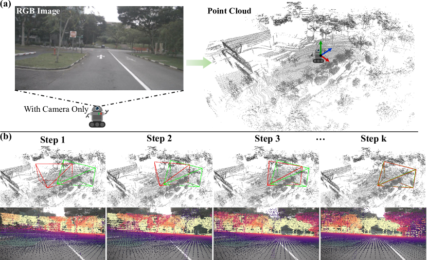
Accurate localization mechanisms are crucial for autonomous driving systems. Although the Global Positioning System (GPS) [1] is widely used, obstacles in real-world environments frequently disrupt the reception of satellite signals, affecting the precision and reliability of localization. To address these challenges, some methods eschew satellite communication and instead use sensors like LiDAR [2] and camera [3] to localize by comparing online sensor measurements with reference maps. Specifically, LiDAR-based methods [4] estimate relative position and rotation by registering online 3D scans with a pre-built point cloud map. They have exhibited superior performance, primarily due to the accurate distance measurements and the immunity to variations in lighting and viewing angles. However, the substantial cost of LiDAR sensors restrict their deployment on micro platforms. Camera-based methods [5] achieve localization by matching and aligning real-time RGB images with previously captured photographs. Despite the economic and lightweight advantages of cameras, these methods are notably susceptible to variations of environmental conditions, such as lighting, weather, and season. Therefore, a question naturally arises: Is it possible to combine the strengths of both LiDAR-based and camera-based techniques by establishing direct connections between RGB images and point cloud maps? As shown in Fig.1 (a), the autonomous driving system can be equipped solely with a low-cost camera for efficient localization in pre-built LiDAR maps, reducing the negative impact of environmental changes on visual-based techniques, since LiDAR maps remain unaffected by such visual discrepancies.
The core of cross-modal localization is to estimate the relative camera pose between an RGB image and a point cloud, commonly termed as image-to-point cloud registration [6]. Most current approaches [7, 8, 9, 10] focus on establishing direct 2D-3D correspondences in feature space, where the feature matching process is conducted only once. These methods are categorized as one-shot registration due to their lack of a feedback mechanism for iterative optimization. Motivated by these concerns, we argue that mimicking the instinctive human process of aligning two objects may enhance the performance of image-to-point cloud registration. It involves iterative observation and adjustment, allowing us to continuously fine-tune the camera pose based on immediate feedback. Accordingly, we reformulate the registration problem as a Markov decision process with multi-step iterations. While reinforcement learning [11] offers an appropriate model to depict this process, migrating it to the cross-modal context remains a complex task.
In this paper, we employ reinforcement learning to develop a Cross-Modal Registration Agent (CMR-Agent) that operates as illustrated in Fig. 1 (b). Our primary focuses are three-fold: 1) How to construct cross-modal state representations? 2) How to guide the training of CMR-Agent? 3) How to improve the efficiency in light of the high time complexity due to repeated iterations? For the first problem, we leverage the current camera pose to project point clouds into 2D grids for pixel-by-pixel feature comparison with RGB images. Since the camera’s field of view is a truncated segment of the 3D space, projections of point clouds from certain poses may not contain any useful information for decision (these states within 2D space are termed as neutral states in Section III-C). To supplement more information, we predict the actual camera frustum in 3D space by point classification and compare it with the camera frustum of the current pose. The final state representation integrates the information from both 2D and 3D space. For the second problem, we use the ground-truth camera pose to back-project 2D pixels into 3D points and design a point-to-point alignment reward function. The total reinforcement loss follows the well-known proximal policy optimization (PPO) algorithm [12], and imitation learning [13] is utilized to initialize the registration policy for quick-start of the training. For the last problem, we observe that a smaller relative pose does not lead to better feature embeddings for point clouds and images. Consequently, the overall framework of CMR-Agent is meticulously crafted to perform one-shot cross-modal embeddings, which are efficiently reused during iteration. It circumvents the repetitive and time-consuming feature extraction. In conclusion, the main contributions are:
-
•
We reformulate image-to-point cloud registration as a Markov Decision process and develop a fully cross-modal registration agent using reinforcement learning and imitation learning.
-
•
We propose a 2D-3D hybrid state representation that efficiently exploits the fine-grained features of images while reducing the useless neutral states.
-
•
We propose a point-to-point alignment reward between the 3D points and the back-projected 2D pixels to guide the training of the agent.
-
•
We design an efficient framework for the agent to reuse the one-shot cross-modal embeddings, decreasing the time complexity of repeated iterations.
Extensive experiments on the KITTI-Odometry [14] and NuScenes [15] datasets show that CMR-Agent outperforms the state-of-the-art methods in registration accuracy. Despite being an iterative method, CMR-Agent demonstrates higher efficiency than some one-shot algorithms, executing 10 iterations in less than 68 milliseconds on a 3090 GPU.
II Related works
II-A Registration between Same Modal Data
Registration plays an important role in camera-based and LiDAR-based localization methods. Image-to-image registration tackles multi-view geometry by estimating the relative pose between two images. The absence of depth information makes the epipolar constraint [16] a classic family of methods for delineating the geometric relationship between pixels across images. Besides, Optical flow [17, 18] and direct feature matching [5, 19] constitute another classic family of methods for visual pose estimation. Point cloud registration seeks to determine the rigid transformation between two point clouds, a process simplified by the presence of 3D geometric information. Methods like Iterative Closest Point (ICP) [20] and its variants [21] are the seminal works to solve this problem. In addition, learning-based feature matching [4, 22] combined with SVD decomposition [23] is also a standard paradigm for point cloud registration. While image-to-image and point cloud registration techniques have achieved satisfactory performance, LiDAR devices are not suitable for micro platforms, and cameras are not robust to changes in environmental conditions.
II-B Cross-Modal Registration
Image-to-point cloud registration combines the advantages of both camera and LiDAR. One of the most popular pipelines is to get 2D-3D point correspondences and then estimate the camera pose using a RANSAC-based PnP solver. 2D3D-MatchNet [7], CorrI2P[8], and CFI2P [9] employ pseudo-siamese neural networks to establish the cross-modal correspondences from 3D points to 2D pixels. In addition, there are some matching-free algorithms. HyperMap[24] converts point clouds into depth maps and proposes a late projection strategy to precompute and compress the 3D map features offline. DeepI2P[6] frames the registration as a two-stage process of point-wise classification and custom pose optimization. EFGHNet[25] utilizes a divide-and-conquer approach, estimating rotation and translation separately by aligning RGB images with 360∘ panoramic depth maps. However, most of these methods are one-shot techniques with limited accuracy. The design of an iterative paradigm has been seldom explored.
II-C Reinforcement Learning in Registration
Reinforcement learning [11] provides a framework to describe the iterative decision-making process. Recent visual pose estimation algorithms [26, 27] leverage reinforcement learning to develop agents that can register two RGB images. Specifically, these image-oriented agents employ a fully convolutional architecture for feature extraction and state representation, outputting actions to iteratively adjust the relative camera pose. As for reinforcement learning-powered point cloud registration, ReAgent [28] employs the PointNet architecture to represent states, progressively moving the source towards the target point clouds. In this study, our goal is to extend reinforcement learning to cross-modal registration between images and point clouds. Direct application of the previous single-modal state representations is not feasible for this task. Additionally, developing training strategies for the agent and improving efficiency pose greater challenges in cross-modal contexts.
III Methodology
III-A Overview
Problem Formulation: In the context of image-to-point cloud registration, denote the scene point cloud as with points and the RGB image as that is taken from the same scene, our goal is to estimate the camera pose when the image was taken. Formally, given the camera intrinsic matrix and , we project P to image plane and get a depth map as:
| (1) | ||||
where is a 3D point and represents a 2D pixel. We encapsulate the entire process of deriving a depth map from the point cloud P into a single function as:
| (2) |
Although and I represent the scene using depth and color, respectively, they are aligned to each other pixel by pixel. Besides, we encapsulate the first two steps in Eq. (1) into another function for point-to-pixel projection as:
| (3) |
Markov Modeling: Previous registration methods take P and I as the observations to derive a camera pose in one step. Inevitably, T shows great deviation from . In this study, we propose to reformulate the one-shot process as a Markov decision process, thereby progressively improving the estimated camera pose. To achieve this, we employ reinforcement learning to train a cross-modal registration agent . For every step , it takes and I as the observations to predict a rigid transformation , and is then applied to to obtain as:
| (4) | ||||
where . These two steps are executed alternately. The accumulation of rigid transformations before the -th step is the current camera pose , which we aim to progressively converge towards as:
| (5) |
Note that each is termed as an action at the -th step, and the calculation of follows the method of disentangled transformation [29] to avoid rotation-induced translation.
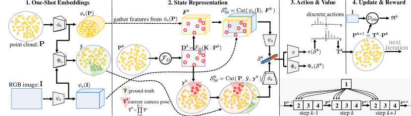
Framework: We implement as a policy network, which uses state representation to predict the distribution of actions. is more complex than the agents for same-modal registration [27, 28] because and I can’t share neural network weights for processing. Although projecting as a depth map can unify the data structure [30], the disparate visual attributes between and I require the network be deeper to achieve sufficient expressive capability, leading to high time complexity when iterating it. To this end, we propose an efficient framework for , as illustrated in Fig.1. We first build a pseudo-siamese neural network to generate one-shot embeddings and for P and I, where is feature dimension. Instead of using and I as the state representation at the -th step, we construct by gathering features from and based on the current camera pose . This design reuses and during iterations, avoiding repetitive and time-consuming feature extraction. After that, a policy head predicts the probability distribution of actions as for decision, and a value head predicts a value as to guide the policy optimization. Once the current camera pose is updated, the agent receives a reward to judge how well it performs.
III-B One-Shot Cross-Modal Embeddings
The goal of the networks and is to map P and I into a unified embedding space while making the correlated 2D pixels and 3D points closer. For this purpose, we adopt circle loss [31] to guide the training. We initially sample 3D points that fall in the camera frustum of pose . Denote the points as and , the corresponding 2D pixels is . For any 3D point , the set of positive 2D pixels is defined as , where is a radius. Conversely, is the negative set. Then, the circle loss anchored in 3D points is formulated as:
| (6) |
where is the distance between and in the embedding space, and , represent the positive and negative margins, respectively. The positive and negative weights are computed adaptively for each samples with and . is a hyper-parameter. Similarly, we get the reverse circle loss in the same way, and the total circle loss is defined as .
Additionally, we follow the previous work [6] to perform point-wise binary classification on P as:
| (7) |
where is the classification head, and any indicates whether the point is within the camera frustum of ground-truth pose . In 3D state representation, will be used to assess the frustum alignment. Note that the prediction of is also a one-shot step. Given as a prior, we obtain the training labels via camera projection and checking whether a 3D point falls into the frustum. We adopt weighted binary cross-entropy as the loss to train .
III-C State Representation
At every step , we first represent the state between and I individually in image plane and point cloud space. Then, we merge the two into a hybrid state representation.
2D State Representation: We project the point cloud onto the image plane as , and assess the alignment between and I. To improve the efficiency of assessment, we reuse the one-shot embeddings and here. Specifically, we first gather the 3D features from to fill the grid of and obtain . For every pixel u, we calculate in as:
| (8) | ||||
where is the feature of point from and represents set cardinality. If , we initialize as a zero vector. Then, the 2D state is represented as:
| (9) |
where refers to the concatenate operation.
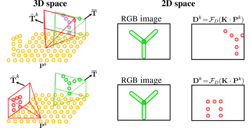
3D State Representation: We found that the 2D state representation is flawed. Because the camera frustum is a truncated segment of the 3D space, there are always certain poses that result in bad cases, i.e., no 3D point associated with the scene in I is contained in the current camera frustum, as illustrated in Fig. 3. In such cases, the 2D states fail to provide any useful information for predicting the action policy, so we term these states as neutral states. To supplement more information, we assess the alignment between the camera frustums of and in 3D space, as illustrated in Fig. 2. The frustum of camera pose is predicted in Eq. (7). Similarly, we also represent the current camera frustum of as binary classification results , where every can be determined by camera projection and checking whether falls into the current frustum. Then, the 3D state is represented as:
| (10) |
2D-3D Hybrid State Representation: To fully exploit the fine-grained features of while reducing the neutral states, we propose to merge both and into a hybrid state representation as:
| (11) |
where and . and are two networks that map the original 2D and 3D states to dimensional state space.
III-D Action Policy
The continuous action space couples degrees of freedom, e.g.., for rotation and for translation. Following the previous method [27], we decompose the action space into orthogonal subspace, and predict the action in each subspace with discrete and limited step size. Taking the -th subspace as an example, our agent predicts the optimal action from a set of candidate actions , where (i.e., is here). Note that the rotation actions are expressed by the angles around different axes. The signs and indicate the direction of the action. Thus, given the state , our agent will predict the action policy as , which are the probability distributions of the candidate actions in all subspace. In the -th subspace, the final action is calculated as:
| (12) |
where represents the probability of action a from . Finally, we adopt the disentangled transformation method [29] to convert the actions into , thereby updating the current camera pose.
III-E Policy Optimization
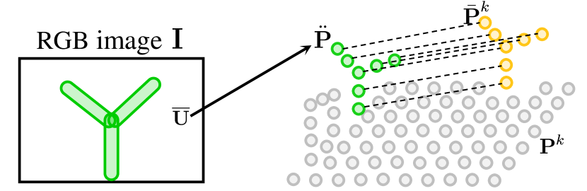
Reward: The goal of the cross-modal registration agent is to align the image and the point cloud as described in Section III-A, therefore, the degree of alignment can serve as a criterion for evaluating the action quality. To quantify it, an intuitive approach is to calculate the average distance between the corresponding pixels in and I, however, it does not work in the neutral states. Instead, we calculate an average distance in 3D space, as illustrated in Fig. 4. Denote the 3D points that fall in the camera frustum of pose as and , they are transformed as at step . The corresponding 2D pixels are defined as . We back-project to 3D space as through the reverse process of Eq. (1). Then, the average distance between and is:
| (13) |
During the process of iterative registration, this distance will become smaller until 0. Inspired by the previous work [28], the step-wise reward is defined as:
| (14) |
where and penalize pausing and divergent actions, and encourages actions that promote alignment.
Optimization: Our agent is based on actor-critic architecture [11] and we adopt the classic proximal policy optimization (PPO) algorithm [12] to optimize the policy. For this purpose, there is also a value head to predict , and the Generalized Advantage Estimation (GAE) [32] is adopted to calculate advantage based on the reward and the value. Following common practices [11], we rollout the trajectories of iterative registration by executing the stochastic policy of the agent and record them in a replay buffer. During training, we gather a batch of random samples from the buffer to update the parameters of agent. The total PPO loss consists of three components: a policy loss for optimizing the policy head , a value loss for optimizing the value head , and an entropy loss of the policy to encourage exploration. For readers unfamiliar with PPO, we recommend referring to the original paper [12] for details.
III-F Quick-Start with Imitation Learning
Learning a cross-modal registration agent from scratch with reinforcement learning will take a long time to converge and might settle into a suboptimal policy. To address these problems, we employ imitation learning [13] to initialize the action policy. As the name suggests, the goal of imitation learning is to mimic the behavior of expert, where the expert could be either a human or another algorithmic approach. Here, we adopt the simplest form of imitation learning, Behavioral Cloning, which takes expert actions as training labels to supervise the action policy of agent. Given as a prior during training, we can easily obtain a greedy expert policy. Specifically, we first calculate the difference between and the current camera pose on the fly as:
| (15) |
After that, we decompose into the optimal actions in subspace as described in Section III-D. In the -th subspace, our greedy expert policy selects the action from the discrete set that is closest to the optimal action mentioned above. Apparently, this is a multi-classification problem, so the imitation learning loss is the cross-entropy between the agent policy and the greedy expert policy.
| KITTI-Odometry-09 (3182 Samples) | KITTI-Odometry-10 (2402 Samples) | NuScenes (16225 Samples) | |||||||
| RTE(m) | RRE(∘) | RR(%) | RTE(m) | RRE(∘) | RR(%) | RTE(m) | RRE(∘) | RR(%) | |
| GridCls [6] | 1.1990.724 | 6.0001.989 | 76.39 | 1.0630.566 | 5.7442.033 | 85.22 | 2.2241.094 | 7.3701.647 | 62.67 |
| DeepI2P(3D) [6] | 1.2260.757 | 6.1132.279 | 39.69 | 1.1780.735 | 6.0402.316 | 36.55 | 1.7300.969 | 7.0582.184 | 18.82 |
| DeepI2P(2D) [6] | 1.4350.918 | 3.8052.660 | 79.73 | 1.3890.862 | 3.9902.727 | 67.57 | 1.9491.050 | 3.0172.285 | 92.53 |
| EFGHNet [25] | 3.0401.269 | 4.5262.347 | 24.18 | 3.0621.297 | 4.7062.371 | 23.57 | 3.9181.493 | 5.7423.439 | 31.25 |
| CorrI2P [8] | 0.9190.742 | 2.4171.988 | 92.65 | 0.8780.689 | 3.1262.333 | 91.59 | 1.6971.030 | 2.3181.868 | 93.87 |
| CFI2P [9] | 0.6100.471 | 1.3611.076 | 99.18 | 0.5740.483 | 1.4381.076 | 99.63 | 1.0930.668 | 1.4651.230 | 99.23 |
| CMR-Agent | 0.1950.151 | 0.5890.843 | 99.94 | 0.2470.210 | 0.7381.089 | 99.63 | 1.0070.680 | 0.9821.337 | 96.96 |
| Param.(MB) | Mem.(GB) | Time(s) | |
|---|---|---|---|
| GridCls [6] | 100.75 | 2.41 | 0.049 |
| DeepI2P(3D) [6] | 100.12 | 2.01 | 16.584 |
| DeepI2P(2D) [6] | 100.12 | 2.01 | 9.381 |
| EFGHNet [25] | 574.32 | 2.76 | 0.319 |
| CorrI2P [8] | 141.07 | 2.88 | 0.088 |
| CFI2P [9] | 34.74 | 2.18 | 0.084 |
| CMR-Agent | 34.65 | 1.87 | 0.068 |
IV Experiments
IV-A Experimental Settings
Implementation Details: All the experiments are conducted on an NVIDIA RTX 3090 GPU. We implement our cross-modal agent with PyTorch 1.12, and train it using the Adam optimizer with an initial learning rate of 0.001 and a momentum of 0.98. The dimension of embedding space is 64. In the one-shot embedding, the positive sample radius is 1 pixel, the number of sampled points is 512, is 10, is 0.1, and is 1.4. The dimension of hybrid state space is 128. In action policy, we suggest using actions with exponential step sizes to quickly cover a large space during early iterations while allowing fine-tuning during later iterations. The set of candidate rotation actions is , the set of candidate translation actions is , and the number of candidates in each subspace is 11. In the reward function, we set to (-0.5, 0, 0.5) empirically. As for training, since CMR-Agent is agnostic to the one-shot cross-modal embedding, we choose to pre-train the backbone separately. Besides, we follow the work [28] to jointly optimize the PPO and imitation learning loss.
Dataset: We conducted experiments on KITTI-Odometry [14] and NuScenes [15] datasets. For KITTI-Odometry, sequences 0-8 are used for training, with sequences 9-10 used for testing. Each data pair consists of a single LiDAR scan as the input point cloud and an RGB image sharing the same frame ID. Each point cloud is downsampled to 40,960 points, and the image resolution is cropped to . For the NuScenes dataset, its official split assigns 850 scenes for training and 150 scenes for testing. Here, multiple LiDAR scans proximate to the frame ID are merged to construct a more comprehensive and uniform point cloud map, alongside selecting the corresponding RGB image. Similarly, this point cloud is sampled to 40,960 points, but the image resolution is cropped to . For a fair comparison, we follow the previous settings [8] to apply a random transformation to the point cloud, consisting of a rotation around the up-axis of up to 360∘ and a translation on the ground within a 10-meter range. It means that and are 1 and 2, respectively. Note that the degrees of freedom can be easily extended to 6D by adjusting the action prediction head.
Evaluation Metrics: We follow the previous work [8] to quantify the performance of image-to-point cloud registration with three metrics: 1) Relative Rotation Error (RRE), 2) Relative Translation Error (RTE), and 3) Registration Recall (RR). RR is the proportion of successful registrations within the test set, with a registration deemed successful when the RRE is less than and the RTE is less than .
IV-B Comparison with the State-of-the-Arts
Baselines: We compare our CMR-Agent with 6 recent algorithms, including the three variants of DeepI2P [6], EFGHNet [25], CorrI2P [8] and CFI2P [9]. Note that EFGHNet is a method based on 360∘ panoramic depth maps, which require good initialization, yet our setup (i.e., 10-meter translation) surpasses the range within which it can work normally. Thus, its performance significantly diverges from what was reported in the original paper [25].
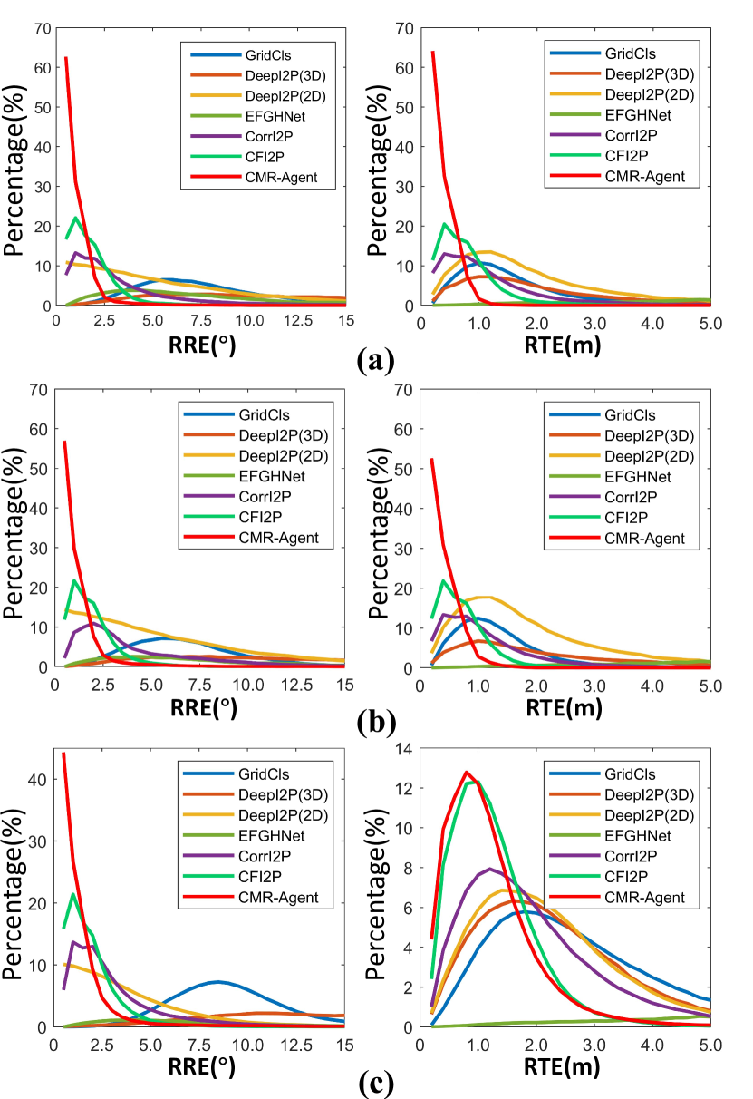
Quantitative Comparison: We report the registration performance of all methods in Table I, where the results of CMR-Agent listed here are from its 10-th iteration, and the thresholds and of RR are set to and m, respectively. These statistical results clearly indicate that our CMR-Agent outperforms the state-of-the-art methods by a large margin. On the KITTI-Odometry dataset, CMR-Agent achieves the highest RR, with an average reduction of about 63% in RRE and about 53% in RTE compared to the suboptimal method CFI2P. On the NuScenes dataset, although RR is slightly lower than that of CFI2P, RRE is reduced by about 8% and RTE is reduced by about 33% on average. For a more comprehensive comparison, we plot the error distributions in Fig. 5, with ranging from 0 to and from 0 to 5 m. The results indicate that our method maintains higher accuracy even with smaller thresholds.
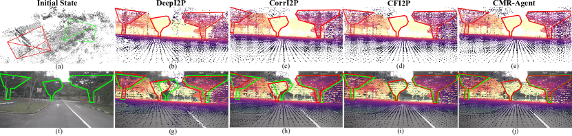
Qualitative Comparison: Image-to-point cloud registration is equivalent to the process of aligning 2D pixels with their corresponding 3D points from the same object. For a more intuitive comparison, we provide a visual example in Fig. 6. Owing to our CMR-Agent’s ability to estimate relative camera poses with minimal error, it also outperforms other methods in achieving superior visual alignment.
Efficiency: The computational resources needed for all methods when executed on the KITTI-Odometry dataset are detailed in Table II. Our CMR-Agent has the minimal number of parameters and the lowest memory footprint during execution. Remarkably, as an iterative method, CMR-Agent completes 10 iterations in just 68 milliseconds, making it the second fastest even when compared to the one-shot methods.
| Method | RTE(m) | RRE(∘) | RR(%) |
|---|---|---|---|
| w/o 3D State | 0.2920.294 | 0.8821.176 | 97.64 |
| w/o 2D State | 0.5260.352 | 2.1071.733 | 99.27 |
| w/o RL Supervision | 0.2600.216 | 0.8911.140 | 99.64 |
| Full Pipeline | 0.2170.181 | 0.6530.959 | 99.80 |
| Iteration | RTE(m) | RRE(∘) | RR(%) | Time(ms) |
|---|---|---|---|---|
| 1 | 2.2721.141 | 4.3462.800 | 23.19 | 0.035 |
| 2 | 1.2131.008 | 3.6042.756 | 52.83 | 0.038 |
| 3 | 0.6630.637 | 2.6492.479 | 78.90 | 0.042 |
| 4 | 0.4260.427 | 1.8442.082 | 95.47 | 0.046 |
| 5 | 0.2910.261 | 1.1381.404 | 99.46 | 0.049 |
| 6 | 0.2360.193 | 0.8141.087 | 99.70 | 0.053 |
| 7 | 0.2220.186 | 0.6910.976 | 99.75 | 0.057 |
| 8 | 0.2180.187 | 0.6790.980 | 99.77 | 0.061 |
| 9 | 0.2170.178 | 0.6580.956 | 99.80 | 0.064 |
| 10 | 0.2170.181 | 0.6530.959 | 99.80 | 0.068 |
IV-C Ablation studies
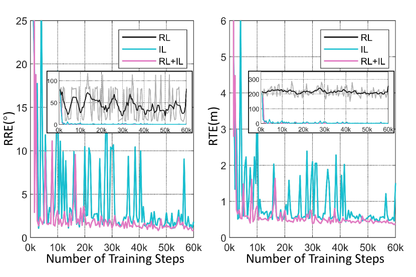
Individual Components: We investigate the contribution of individual components by removing them from the full pipeline of CMR-Agent. The results are listed in Table III. By simply removing the 3D state representation, we can see that RR has dropped significantly compared to the other three rows. This serves as a significant evidence that neutral states (see Section. III-C) exist and fail to provide useful information for action decision. By simply removing the 2D state representation, we can see that RR still maintains a relatively high value, while RTE and RRE have significantly increased. This demonstrates that the 3D state supplements useful information to 2D neutral states, yet its contribution to fine registration is less than that provided by the fine-grained features of RGB images. Thus, the results in the first two rows of Table III demonstrate the necessity of the 2D-3D hybrid state representation. In addition, we also investigate the role of reinforcement learning (RL) and imitation learning (IL) by training our CMR-Agent both separately and jointly. The curves of validation error are displayed in Fig .7. When trained solely with RL, in line with the prior experience [27, 28], the convergence process is very slow. IL promotes quick convergence but suffers from training instability and limited accuracy. The main bottleneck lies in the greedy expert policy, and theoretically, it is impossible for the agent to learn a policy better than the expert. As shown in Fig.7 and the last two rows of Table. III, the combination of IL and RL results in training that is both rapid and stable, breaking through the accuracy limitation of IL.
Number of Iterations: We iterate CMR-Agent for different numbers of times and report the results in Table IV. Obviously, the registration performance positively correlates with the number of iterations, and CMR-Agent only takes 34 ms per iteration once the one-shot embeddings are completed. A dynamic demonstration of the entire iterative process is included at the end of the supplementary video.
V Conclusion
In this paper, we propose a novel cross-modal agent (CMR-Agent) for image-to-point cloud registration. Our key insight is to mimic the natural human process of aligning two objects through observation and adjustment. By reformulating the problem as a Markov decision process, we implement CMR-Agent with reinforcement learning. The proposed 2D-3D hybrid state representation fully exploits the fine-grained features of RGB images while reducing the useless neutral states. The proposed point-to-point alignment reward bridges the modality gap between images and point clouds to guide the training. The proposed framework for reusing one-shot embeddings also makes CMR-Agent very efficient. Extensive experiments demonstrate notable improvements in registration performance, showcasing the great potential of our method to achieve accurate camera localization in pre-built LiDAR maps.
References
- [1] Bernhard Hofmann-Wellenhof, Herbert Lichtenegger, and James Collins, Global positioning system: theory and practice, Springer Science & Business Media, 2012.
- [2] Lucas de Paula Veronese, Fernando Auat-Cheein, Filipe Mutz, and et al., “Evaluating the limits of a lidar for an autonomous driving localization,” IEEE Transactions on Intelligent Transportation Systems, vol. 22, no. 3, pp. 1449–1458, 2020.
- [3] Changhao Chen, Bing Wang, Chris Xiaoxuan Lu, and et al., “Deep learning for visual localization and mapping: A survey,” IEEE Transactions on Neural Networks and Learning Systems, 2023.
- [4] Shengyu Huang, Zan Gojcic, Mikhail Usvyatsov, Andreas Wieser, and Konrad Schindler, “Predator: Registration of 3d point clouds with low overlap,” in IEEE/CVF Conference on Computer Vision and Pattern Recognition, 2021, pp. 4267–4276.
- [5] J. Sun, Z. Shen, Y. Wang, H. Bao, and X. Zhou, “Loftr: Detector-free local feature matching with transformers,” in Computer Vision and Pattern Recognition, 2021.
- [6] Jiaxin Li and Gim Hee Lee, “Deepi2p: Image-to-point cloud registration via deep classification,” in IEEE/CVF Conference on Computer Vision and Pattern Recognition, 2021, pp. 15960–15969.
- [7] Mengdan Feng, Sixing Hu, Marcelo H Ang, and Gim Hee Lee, “2d3d-matchnet: Learning to match keypoints across 2d image and 3d point cloud,” in 2019 International Conference on Robotics and Automation (ICRA). IEEE, 2019, pp. 4790–4796.
- [8] Siyu Ren, Yiming Zeng, Junhui Hou, and Xiaodong Chen, “Corri2p: Deep image-to-point cloud registration via dense correspondence,” IEEE Transactions on Circuits and Systems for Video Technology, vol. 33, no. 3, pp. 1198–1208, 2023.
- [9] Gongxin Yao, Yixin Xuan, Yiwei Chen, and Yu Pan, “CFI2P: Coarse-to-fine cross-modal correspondence learning for image-to-point cloud registration,” arXiv preprint arXiv:2307.07142, 2023.
- [10] Shuhang Zheng, Yixuan Li, Zhu Yu, and et al., “I2p-rec: Recognizing images on large-scale point cloud maps through bird’s eye view projections,” in 2023 IEEE/RSJ International Conference on Intelligent Robots and Systems (IROS). IEEE, 2023, pp. 1395–1400.
- [11] Csaba Szepesvári, Algorithms for reinforcement learning, Springer Nature, 2022.
- [12] John Schulman, Filip Wolski, Prafulla Dhariwal, and et al., “Proximal policy optimization algorithms,” arXiv preprint arXiv:1707.06347, 2017.
- [13] Abdoulaye O Ly and Moulay Akhloufi, “Learning to drive by imitation: An overview of deep behavior cloning methods,” IEEE Transactions on Intelligent Vehicles, vol. 6, no. 2, pp. 195–209, 2020.
- [14] Andreas Geiger, Philip Lenz, Christoph Stiller, and Raquel Urtasun, “Vision meets robotics: The kitti dataset,” The International Journal of Robotics Research, vol. 32, no. 11, pp. 1231–1237, 2013.
- [15] Holger Caesar, Varun Bankiti, Alex H Lang, and et al., “nuscenes: A multimodal dataset for autonomous driving,” in IEEE/CVF Conference on Computer Vision and Pattern Recognition, 2020, pp. 11621–11631.
- [16] Qunjie Zhou, Torsten Sattler, and Laura Leal-Taixe, “Patch2pix: Epipolar-guided pixel-level correspondences,” in IEEE/CVF Conference on Computer Vision and Pattern Recognition, 2021, pp. 4669–4678.
- [17] Mingliang Zhai, Xuezhi Xiang, Ning Lv, and Xiangdong Kong, “Optical flow and scene flow estimation: A survey,” Pattern Recognition, vol. 114, pp. 107861, 2021.
- [18] Yawen Lu, Qifan Wang, Siqi Ma, and et al., “Transflow: Transformer as flow learner,” in IEEE/CVF Conference on Computer Vision and Pattern Recognition, 2023, pp. 18063–18073.
- [19] Tao Xie, Kun Dai, Ke Wang, and et al., “Deepmatcher: a deep transformer-based network for robust and accurate local feature matching,” Expert Systems with Applications, vol. 237, pp. 121361, 2024.
- [20] P.J. Besl and Neil D. McKay, “A method for registration of 3-d shapes,” IEEE Transactions on Pattern Analysis and Machine Intelligence, vol. 14, no. 2, pp. 239–256, 1992.
- [21] Jiaolong Yang, Hongdong Li, and Yunde Jia, “Go-icp: Solving 3d registration efficiently and globally optimally,” in IEEE International Conference on Computer Vision, 2013, pp. 1457–1464.
- [22] Zheng Qin, Hao Yu, Changjian Wang, and et al., “Geotransformer: Fast and robust point cloud registration with geometric transformer,” IEEE Transactions on Pattern Analysis and Machine Intelligence, 2023.
- [23] Théodore Papadopoulo and Manolis IA Lourakis, “Estimating the jacobian of the singular value decomposition: Theory and applications,” in Computer Vision-ECCV 2000: 6th European Conference on Computer Vision Dublin, Ireland, June 26–July 1, 2000 Proceedings, Part I 6. Springer, 2000, pp. 554–570.
- [24] Ming-Fang Chang, Joshua Mangelson, Michael Kaess, and Simon Lucey, “Hypermap: Compressed 3d map for monocular camera registration,” in 2021 IEEE International Conference on Robotics and Automation (ICRA), 2021, pp. 11739–11745.
- [25] Yurim Jeon and Seung-Woo Seo, “EFGHNet: A versatile image-to-point cloud registration network for extreme outdoor environment,” IEEE Robotics and Automation Letters, vol. 7, no. 3, pp. 7511–7517, 2022.
- [26] Alexander Krull, Eric Brachmann, Sebastian Nowozin, and et al., “Poseagent: Budget-constrained 6d object pose estimation via reinforcement learning,” in IEEE Conference on Computer Vision and Pattern Recognition (CVPR), July 2017.
- [27] Jianzhun Shao, Yuhang Jiang, Gu Wang, Zhigang Li, and Xiangyang Ji, “Pfrl: Pose-free reinforcement learning for 6d pose estimation,” in IEEE/CVF Conference on Computer Vision and Pattern Recognition (CVPR), June 2020.
- [28] Dominik Bauer, Timothy Patten, and Markus Vincze, “Reagent: Point cloud registration using imitation and reinforcement learning,” in IEEE/CVF Conference on Computer Vision and Pattern Recognition, 2021, pp. 14586–14594.
- [29] Yi Li, Gu Wang, Xiangyang Ji, and et al., “Deepim: Deep iterative matching for 6d pose estimation,” in European Conference on Computer Vision (ECCV), 2018, pp. 683–698.
- [30] Daniele Cattaneo, Matteo Vaghi, Augusto Ballardini, and et al., “Cmrnet: Camera to lidar-map registration,” in 2019 IEEE intelligent transportation systems conference (ITSC). IEEE, 2019, pp. 1283–1289.
- [31] Yifan Sun, Changmao Cheng, Yuhan Zhang, and et al., “Circle loss: A unified perspective of pair similarity optimization,” in IEEE/CVF Conference on Computer Vision and Pattern Recognition, 2020, pp. 6398–6407.
- [32] John Schulman, Philipp Moritz, Sergey Levine, and et al., “High-dimensional continuous control using generalized advantage estimation,” arXiv preprint arXiv:1506.02438, 2015.