Impact of the Electroweak Weinberg Operator
on the Electric Dipole Moment of Electron

Abstract

Recent progresses in the measurements of the electric dipole moment (EDM) of the electron using the paramagnetic atom or molecule are remarkable. In this paper, we calculate a contribution to the electron EDM at three-loop level, introducing the CP-violating Yukawa couplings of new SU(2)_L multiplets. At two-loop level, the Yukawa interactions generate a CP-violating dimension-six operator, composed of three SU(2)_L field strengths, called the electroweak Weinberg operator. Another one-loop diagram with the operator inserted induces the electron EDM. We find that even if new SU(2)_L particles have masses around TeV-scale, the electron EDM may be larger than the Standard Model contribution to the paramagnetic atom or molecule EDMs. We also discuss the relation between the Barr-Zee diagram contribution at two-loop level and the three-loop one, assuming that the SM Higgs has new Yukawa interactions with the SU(2)_L multiplets.

1   Introduction

The experimental sensitivities on the electric dipole moment (EDM) of the electron ($d_{e}$) have been remarkably improved by new technology since 2010’s. The Imperial College experiment using the YbF molecules surpassed the limits set by atoms, such as Tl, and they reached to $|d_{e}|<1.05\times 10^{-27}e\,{\rm cm}$ in 2011 Hudson:2011zz . The bound was quickly updated by the ACME experiment using the ThO molecules as $|d_{e}|<8.7\times 10^{-29}{e}\,{\rm cm}$ in 2013 ACME:2013pal , and also they reached $1.1\times 10^{-29}{e}\,{\rm cm}$ in 2018 ACME:2018yjb . In 2023 Roussy:2022cmp , the JILA HfF⁺ experiment gives the current world record as $|d_{e}|<4.1\times 10^{-30}e\,{\rm cm}$. It is expected, as reported in Ref. Alarcon:2022ero , that the electron EDM will be further improved by several orders of magnitude in the next decades.

The upper bound on the electron EDM gives a severe constraint on the physics beyond the standard model (BSM), if they have $O(1)$ CP-violating interactions; the BSM models responsible for the matter-antimatter asymmetry in the Universe are required to have $O(1)$ CP-violating interactions. The neutrino oscillation experiments have been suggesting that the CP phase in the Pontecorvo-Maki-Nakagawa-Sakata (PMNS) matrix may be $O(1)$ T2K:2019bcf ; T2K:2023smv ; NOvA:2023iam . They might mean that the CP-violating interactions are ubiquitous in BSM models. The electron EDM is induced by loop diagrams with CP-violating interactions if the perturbation theories are applicable, and it is proportional to the electron mass ($m_{e}$) in typical BSM models. Thus, the electron EDM is approximately given as

$$\frac{d_{e}}{e} \approx\left(\frac{\bar{g}^{2}}{16\pi^{2}}\right)^{n}\frac{m_{e}}{\Lambda^{2}}\sin\phi_{\rm CP}\,,$$ (1.1)

if the $n$-loop diagrams generate it. If we take the coupling constant $\bar{g}$ to be comparable to the SU(2)_L and the CP-violating phase $\phi_{\rm CP}$ is $O(1)$, the current electron EDM bound gives the BSM scale $\Lambda$ as $\Lambda\gtrsim 80$ TeV for the one-loop and $\Lambda\gtrsim 4$ TeV for the two-loop level. If the BSM is assumed to be around the TeV scale and to have $O(1)$ CP-violating phases, we have to tune the BSM models so that the electron EDM is suppressed below the bound.

One of the typical two-loop contributions to the electron EDM in the BSM models is the Barr-Zee diagrams Barr:1990vd ; If the SM Higgs boson $h$ has the CP-violating Yukawa or higher-dimensional couplings with the BSM fermions, the dimension-five CP-violating $h$-$\gamma$-$\gamma$ coupling is generated by one-loop diagrams, and it induces the electron EDM by another one loop. If the dark matter in the Universe is a neutral component in an SU(2)_L multiplet, its mass is expected to be around TeV scale from the thermal decoupling hypothesis Cirelli:2005uq ; Hisano:2006nn ; Cirelli:2007xd ; Cirelli:2009uv . Note that all the charged components in the SU(2)_L multiplets receive constructive radiative corrections to the masses, which is $\mathcal{O}(100)\,$MeV, so that the neutral component is automatically the lightest particle in the multiplet Cirelli:2005uq . Then, their CP-violating couplings with the SM Higgs boson are constrained by the current electron EDM measurements Hisano:2014kua ; Nagata:2014wma .

In the next decades, the electron EDM sensitives will be improved, as mentioned above. It is expected that even the three-loop contributions will be tested there. If SU(2)_L multiplet fermions and/or scalars in the BSM models have CP-violating Yukawa couplings, the two-loop diagrams generate the dimension-six CP-violating operator composed of the SU(2)_L field-strengths, which is given as Here, $W_{\mu\nu}^{a}$ ($a=1$–$3$) are the SU(2)_L field-strengths, $\theta_{w}$ is the weak-mixing angle and $g$ and $\epsilon^{abc}$ are the SU(2)_L gauge coupling constant and structure constants, respectively. The $C_{W}$ is the Wilson coefficient. The operator in QCD is called the Weinberg operator. Then, we call the operator in Eq. (LABEL:eq:Weinberg_operator) as the electroweak Weinberg operator in this paper. The electroweak Weinberg operator is given by the field strengths of $W$ boson ($W^{\pm}_{\mu\nu}$) and photon (${F}_{\mu\nu}$) or $Z$ boson ($Z_{\mu\nu}$) as given in the second line of Eq. (LABEL:eq:Weinberg_operator). The electroweak Weinberg operator contributes to the EDM and magnetic quadrupole moment of the $W$ boson, which can be probed by the collider experiments CMS:2021foa , referred to as the anomalous $WW\gamma$ coupling Hagiwara:1986vm . In addition, it also contributes to the electron EDM at one-loop level Boudjema:1990dv ,

$$\frac{d_{e}}{e} =\frac{1}{2}\left(\alpha_{2}\right)^{2}m_{e}C_{W}\,,$$ (1.2)

where $\alpha_{2}=g^{2}/4\pi$, and hence the electroweak Weinberg operator is much severely constrained by the electron EDM measurements.

In this paper, we evaluate the electron EDM induced by the electroweak Weinberg operator in the BSM models where the SU(2)_L fermions and/or scalar with TeV scale masses have CP-violating Yukawa couplings. Such particles are nowadays motivated by the dark matter as mentioned above, though we do not necessarily assume any dark matter models in this paper since our results are applicable to a wider class of BSM models. In those models, they may have the Yukawa coupling to get their masses. From a viewpoint of stability of the dark matter, the fermion SU(2)_L representation is favored to the five-dimensional multiplet ($r=5$) or more, or the scalar is the seven-dimensional one ($r=7$) Cirelli:2005uq ; Cirelli:2007xd ; Cirelli:2009uv ; such large SU(2)_L representations automatically lead to an accidental symmetry for the dark matter stability within renormalizable theories. Interestingly, we find that they also lead to an enhancement of the electron EDM, proportional to $r^{3}$.

The electron EDM is measured using paramagnetic atoms or molecules in the current experiments. The CP-violating semi-leptonic four-Fermi operators also contribute to them in addition to the electron EDM. The SM contribution from the four-Fermi operators is equivalent to $d_{e}^{\rm eq}=1.0\times 10^{-35}e\,{\rm cm}$ Ema:2022yra . When the BSM contributions to the electron EDM are smaller than $d_{e}^{\rm eq}$, it is difficult to extract the BSM contribution from the observed value. We find that the electroweak Weinberg operator contributes to the electron EDM being larger than $d_{e}^{\rm eq}$, even if the BSM particle masses are around the TeV scale.

We do not evaluate the electroweak Weinberg operator contribution to the light quark EDMs, though the calculation is straight-forward. They contribute to the hadronic EDMs, such as the neutron and Mercury ones. However, the electron EDM constrains the electroweak Weinberg operator much severely, and the hadronic EDM measurements are not competitive with the electron EDM even in their future prospects.

This paper is organized as follows. In Sec. 2, we review the Weinberg operator in SU($N$) gauge theories generated by the CP-violating Yukawa couplings of the heavier particles. We follow the results in Ref. Abe:2017sam , while the analytic formulae are given there. In Sec. 3, we show the contributions to the electron EDM from the electroweak Weinberg operator. Since there were some confusions in the evaluation, we rederive it there. In Sec. 4, the numerical results are shown. In this paper, we assume that the BSM particles are heavier than the $W$ boson so that the effective theory description with the electroweak Weinberg operator works. We also discuss the relations between the Barr-Zee diagrams and the electroweak Weinberg operator contributions. The Barr-Zee diagrams are generated at two-loop level if the SM Higgs boson has the CP-violating Yukawa coupling. The radiative corrections to the Barr-Zee diagrams are evaluated in Ref. Kuramoto:2019yvj , while they might be comparable to the electroweak Weinberg operator contribution to the electron EDM. Section 5 is devoted to conclusions.

2   Weinberg operator in SU($N$) gauge theory at two-loop level

The Weinberg operator was originally introduced in the SU(3)_C. It can be extended in the SU($N$) gauge theories as

$$\mathcal{L}_{W}=-\frac{g^{3}}{3}C_{W}f^{abc}W^{a}_{\mu\nu}W^{b\nu}_{\leavevmode\nobreak\ \ \rho}\widetilde{W}^{c\rho\mu}\,.$$ (2.1)

Here, $g$, $f^{abc}$, and $W^{a}_{\mu\nu}$ are the gauge coupling constant, the structure constant, and the field strength of SU($N$) gauge theory, respectively, and its dual is $\widetilde{W}^{a\mu\nu}=\frac{1}{2}\varepsilon^{\mu\nu\rho\sigma}W^{a}_{\rho\sigma}$ with $\varepsilon^{0123}=+1$.

Figure 1: Two-loop diagrams contributing to the SU($N$) Weinberg operator.

The Weinberg operator is generated by the CP-violating Yukawa couplings at two-loop level, see Fig. 1. First, we consider renormalizable Yukawa interactions between fermions ($\psi_{A}$ and $\psi_{B}$) and a complex scalar field ($S$) as follows:

$$\mathcal{L}\supset-\bar{\psi}_{B}g_{\bar{B}AS}\psi_{A}S-\bar{\psi}_{A}g_{\bar{A}B\bar{S}}\psi_{B}S^{*}\,,$$ (2.2)

where

$$g_{\bar{B}AS} =X_{\bar{B}AS}(s+\gamma_{5}a)\,,$$ (2.3)

$$g_{\bar{A}B\bar{S}} =X_{\bar{A}B\bar{S}}(s^{*}-\gamma_{5}a^{*})\,.$$ (2.4)

Here, $X$s are the SU($N$) invariant tensors, which depend on the representations of the fields, and $s$ and $a$ are arbitrary complex numbers. In Table 1, the representative forms of $X_{\bar{B}AS}$ are listed.

$(A,B,S)$	$\psi_{A}\psi_{B}S$	$X_{\bar{B}AS}$	$XT_{A}T_{A}X^{\dagger}$	$XT_{A}X^{\dagger}T_{B}$	$XX^{\dagger}T_{B}T_{B}$
$(N,N,1)$	$(\psi_{A})_{a}(\psi_{B})_{b}S$	$\delta^{ab}$	$1/2$	$1/2$	$1/2$
$(N,1,\bar{N})$	$(\psi_{A})_{a}\psi_{B}S_{i}$	$\delta^{ai}$	$1/2$	$0$	$0$
$(\bar{N},N,{\square\square})$	$(\psi_{A})_{a}(\psi_{B})_{b}S_{ij}$	$(\delta^{b}_{i}\delta^{a}_{j}+\delta^{b}_{j}\delta^{a}_{i})/2$	$(N+1)/4$	$-1/4$	$(N+1)/4$
$(N,N,\text{Ad})$	$(\psi_{A})_{i}(\psi_{B})_{j}S^{a}$	$(T_{N}^{a})^{j}_{\leavevmode\nobreak\ i}$	$(N^{2}-1)/4N$	$-1/4N$	$(N^{2}-1)/4N$
$(N,\text{Ad},\bar{N})$	$(\psi_{A})_{i}(\psi_{B})^{a}S_{j}$	$(T_{N}^{a})^{j}_{\leavevmode\nobreak\ i}$	$(N^{2}-1)/4N$	$N/4$	$N/2$
$(\text{Ad},\text{Ad},1)$	$(\psi_{A})_{a}(\psi_{B})_{b}S$	$\delta^{ab}$	$N$	$N$	$N$
$(\text{Ad},1,\text{Ad})$	$(\psi_{A})_{a}\psi_{B}S_{i}$	$\delta^{ai}$	$N$	$0$	$0$
$(\text{Ad},\text{Ad},\text{Ad})$	$(\psi_{A})_{a}(\psi_{B})_{b}S_{i}$	$f^{bai}$	$N^{2}$	$f^{a}_{\leavevmode\nobreak\ AA^{\prime}}f^{i}_{\leavevmode\nobreak\ A^{\prime}B^{\prime}}f^{b}_{\leavevmode\nobreak\ B^{\prime}B}f^{i}_{\leavevmode\nobreak\ BA}$	$N^{2}$

Table 1: Group factors in typical SU($N$) representations. The Young Tableau ${\square\square}$ is the minimal symmetric ($N(N+1)/2$) representation, while $N$ and Ad stand for the fundamental and adjoint representations.

The Wilson coefficient $C_{W}$ was evaluated in the SU(3)_C case presented in Ref. Abe:2017sam using the Fock-Schwinger gauge method Fock:1937dy ; Schwinger:1951nm ; key86364857 ; Cronstrom:1980hj ; Shifman:1980ui ; Dubovikov:1981bf ; Novikov:1983gd . From the result, we obtain $C_{W}$ as

$$C_{W} =\frac{6}{(4\pi)^{4}}\mathop{\mathrm{Im}}(sa^{*})m_{A}m_{B}$$

$$\ \times\bigg{\{}\left(XT_{A}T_{A}X^{\dagger}\right)g_{1}(m_{A}^{2},m_{B}^{2},m_{S}^{2})+\left(XX^{\dagger}T_{B}T_{B}\right)g_{1}(m_{B}^{2},m_{A}^{2},m_{S}^{2})$$

$$\qquad+\left(XT_{A}X^{\dagger}T_{B}\right)\left[g_{2}(m_{A}^{2},m_{B}^{2},m_{S}^{2})+g_{2}(m_{B}^{2},m_{A}^{2},m_{S}^{2})\right]\bigg{\}}\,.$$ (2.14)

Here, the group factors are defined as

$$\left(XT_{A}T_{A}X^{\dagger}\right)\delta^{ab} =\left(X_{\bar{B}AS}(T^{a})_{AA^{\prime}}(T^{b})_{A^{\prime}A^{\prime\prime}}X^{\dagger}_{\bar{A}^{\prime\prime}B\bar{S}}\right)\,,$$ (2.15)

$$\left(XX^{\dagger}T_{B}T_{B}\right)\delta^{ab} =\left(X_{\bar{B}AS}X^{\dagger}_{\bar{A}B^{\prime\prime}\bar{S}}(T^{a})_{B^{\prime}B^{\prime\prime}}(T^{b})_{B^{\prime\prime}B}\right)\,,$$ (2.16)

$$\left(XT_{A}X^{\dagger}T_{B}\right)\delta^{ab} =\left(X_{\bar{B}AS}(T^{a})_{AA^{\prime}}X^{\dagger}_{\bar{A}^{\prime}B^{\prime}\bar{S}}(T^{b})_{B^{\prime}B}\right)\,,$$ (2.17)

and the subscript of $T^{a}$, such as $A$ or $B$, denotes that it is the generator for the fermion field $A$ or $B$ with $a=1,2,\cdots,N^{2}-1$. In Table 1, we show the explicit values of the group factors for typical SU$(N)$ representations. The two-loop functions $g_{1}$ and $g_{2}$ are defined as

$$g_{1}(x_{1},x_{2},x_{3}) =\left(2\bar{I}_{(4;1)}+4x_{1}\bar{I}_{(5;1)}\right)(x_{1};x_{2};x_{3})\,,$$ (2.18)

$$g_{2}(x_{1},x_{2},x_{3}) =\left(\bar{I}_{(3;2)}+x_{1}\bar{I}_{(4;2)}\right)(x_{1};x_{2};x_{3})\,,$$ (2.19)

where $\bar{I}_{(n;m)}$ is the UV finite two-loop function, which is given as

$$\bar{I}_{(n;m)}(x_{1};x_{2};x_{3})=\frac{1}{(n-1)!(m-1)!}\frac{d^{n-1}}{dx_{1}^{n-1}}\frac{d^{m-1}}{dx_{2}^{m-1}}\bar{I}(x_{1};x_{2};x_{3})\,,$$ (2.20)

and the explicit form of $\bar{I}$ is

$$\bar{I}(x_{1};x_{2};x_{3})=-\frac{1}{2}\biggl{[}(-x_{1}+x_{2}+x_{3})\log\frac{x_{2}}{Q^{2}}\log\frac{x_{3}}{Q^{2}}+(x_{1}-x_{2}+x_{3})\log\frac{x_{1}}{Q^{2}}\log\frac{x_{3}}{Q^{2}}$$

$$\quad+(x_{1}+x_{2}-x_{3})\log\frac{x_{1}}{Q^{2}}\log\frac{x_{2}}{Q^{2}}-4\left(x_{1}\log\frac{x_{1}}{Q^{2}}+x_{2}\log\frac{x_{2}}{Q^{2}}+x_{3}\log\frac{x_{3}}{Q^{2}}\right)$$

$$\quad+5(x_{1}+x_{2}+x_{3})+\xi(x_{1},x_{2},x_{3})\biggr{]}\,,$$ (2.21)

and

$$\xi(x_{1},x_{2},x_{3})=R\left[2\log\left(\frac{x_{3}+x_{1}-x_{2}-R}{2x_{3}}\right)\log\left(\frac{x_{3}-x_{1}+x_{2}-R}{2x_{3}}\right)-\log\frac{x_{1}}{x_{3}}\log\frac{x_{2}}{x_{3}}\right.$$

$$\quad\left.-2{\rm Li}_{2}\left(\frac{x_{3}+x_{1}-x_{2}-R}{2x_{3}}\right)-2{\rm Li}_{2}\left(\frac{x_{3}-x_{1}+x_{2}-R}{2x_{3}}\right)+\frac{\pi^{2}}{3}\right]\,,$$ (2.22)

where $R=\sqrt{x_{1}^{2}+x_{2}^{2}+x_{3}^{2}-2x_{1}x_{2}-2x_{2}x_{3}-2x_{3}x_{1}}$ and $Q^{2}=4\pi\mu^{2}e^{-\gamma_{E}}$Ford:1992pn ; Espinosa:2000df ; Martin:2001vx . Here, we introduce the dimensional regularization $d=4-2\epsilon$ with renormalization scale $\mu$, and we adopt the $\overline{\text{MS}}$ subtraction scheme. This is because the subdiagrams contain UV-divergence though the final result is UV-finite. In Ref. Abe:2017sam , $g_{1}$ and $g_{2}$ are numerically evaluated. Since we use the analytic mass function for the two-loop vacuum diagram, $\bar{I}(x_{1};x_{2};x_{3})$, we can evaluate them analytically. For more details about the two-loop function, see Ref. Hisano:2023izx .

The analytic formula for $C_{W}$ is useful in the discussion of the behavior in decoupling of the heavy particles. When $m_{A}\ll m_{B}$ and $m_{S}$, the following effective theory approach works in the evaluation of the SU($N$) Weinberg operator. First, the SU($N$) EDM of the lighter fermion $\psi_{A}$ is generated at one-loop level by integrating $\psi_{B}$ and $S$ out, as follows:

$$\begin{aligned} d_{A}^{N}=&-\frac{1}{(4\pi)^{2}}\mathop{\mathrm{Im}}(sa^{*})(X^{\dagger}T_{S}X)\frac{m_{B}}{m_{S}^{2}}f_{S}(x_{BS})\\ &-\frac{1}{(4\pi)^{2}}\mathop{\mathrm{Im}}(sa^{*})(X^{\dagger}T_{B}X)\frac{m_{B}}{m_{S}^{2}}f_{B}(x_{BS})\,,\end{aligned}$$ (2.23)

where $x_{BS}=m_{B}^{2}/m_{S}^{2}$ and

$$f_{S}(x) =\frac{1-x^{2}+2x\log x}{(1-x)^{3}}\,,$$ (2.24)

$$f_{B}(x) =-\frac{3-4x+x^{2}+2\log x}{(1-x)^{3}}\,.$$ (2.25)

The group factors are given as

$$(X^{\dagger}T_{S}X)(T^{a})_{AA^{\prime}} =\left(X^{\dagger}_{\bar{A}BS}(T^{a})_{SS^{\prime}}X_{\bar{B}A^{\prime}S^{\prime}}\right)\,,$$ (2.26)

$$(X^{\dagger}T_{B}X)(T^{a})_{AA^{\prime}} =\left(X^{\dagger}_{\bar{A}BS}(T^{a})_{BB^{\prime}}X_{\bar{B}^{\prime}A^{\prime}S}\right)\,.$$ (2.27)

Next when $\psi_{A}$ is decoupled, the SU($N$) Weinberg operator is induced at one-loop level from the operator of $d_{A}^{N}$, as

$$C_{W}=\frac{1}{(4\pi)^{2}}N(r_{A})\frac{d_{A}^{N}}{m_{A}}\,.$$ (2.28)

where the Dynkin index $N(r)$ is defined by ${\rm tr}(T^{a}T^{b})=N(r)\delta^{ab}$. This is directly derived from the analytical formula in Eq. (2.14) by taking $m_{A}\ll m_{B}$ and $m_{S}$. In this case, the mass functions are approximately given as

$$g_{1}(m_{A}^{2},m_{B}^{2},m_{S}^{2}) \simeq\frac{1}{6m_{A}^{2}m_{S}^{2}}f_{S}(x_{BS})\,,$$ (2.29)

$$g_{2}(m_{A}^{2},m_{B}^{2},m_{S}^{2}) \simeq-\frac{1}{6m_{A}^{2}m_{S}^{2}}\left[f_{S}(x_{BS})+f_{B}(x_{BS})\right]\,.$$ (2.30)

In $C_{W}$, $g_{1/2}(m_{B}^{2},m_{A}^{2},m_{S}^{2})$ are negligible compared with $g_{1/2}(m_{A}^{2},m_{B}^{2},m_{S}^{2})$. Since $X$ is an invariant tensor in SU($N$), we get Abe:2017sam

$$XT_{A}T_{A}X^{\dagger} =N(r_{A})(X^{\dagger}T_{B}X-X^{\dagger}T_{S}X)\,,$$ (2.31)

$$XT_{A}X^{\dagger}T_{B} =N(r_{A})X^{\dagger}T_{B}X\,.$$ (2.32)

Using the above formulae, we can derive Eq. (2.28). From the above exercise, we found that when one of the fermions is lighter, the Weinberg operator is enhanced by the lighter mass; a factor of $m_{B}/m_{A}$ in this case.

When $m_{S}\gg m_{B}>m_{A}$, integration of $S$ generates SU($N$) EDMs for $\psi_{A}$ and $\psi_{B}$ in addition to the CP-violating four-Fermi operator of $\psi_{A}$ and $\psi_{B}$ Banno:2023yrd . The SU($N$) EDMs are proportional to $m_{B}/m_{S}^{2}$ and $m_{A}/m_{S}^{2}$, respectively. The SU($N$) EDMs and the four-Fermi operator are mixed due to their anomalous dimensions Hisano:2012cc . Integration of $\psi_{A}$ and $\psi_{B}$ generate the Weinberg operator proportional to the physical SU($N$) EDMs as explained above. Then, the dominant contribution is proportional to $(m_{B}/m_{A})/m_{S}^{2}\log(m_{S}^{2}/m_{B}^{2})$ when $m_{S}\gg m_{B}>m_{A}$. The logarithmic enhancement appears in Eq. (2.25).

In this section we discussed the Weinberg operator in SU($N$) gauge theories. We assumed that the SU($N$) gauge-boson mass is negligible in the two-loop contributions to the Weinberg operator in Eq. (2.14). In the next section, we consider the electroweak Weinberg operator and apply the above results to the evaluation of electron EDM. This implies that the BSM particles in the CP-violating Yukawa couplings are heavy enough for the $W$ boson to be negligible.

For later convenience, in Table 2 we listed the explicit group factors in the SU(2)_L representations. We also obtain the general formulae of the group factors for the $(A,B,S)=(r,r,1)$ and $(r,1,r)$ representations. They correspond to the Dynkin index $N(r)=r(r^{2}-1)/12$ which can be obtained from the quadratic Casimir operator $C_{2}(r)\delta_{ij}(\equiv(T^{a}T^{a})_{ij})=((r^{2}-1)/4)\delta_{ij}$. Notably, it is important for this paper that the group factors are enhanced by the cubic power of $r$, which amplifies the electroweak Weinberg operator.

$(A,B,S)$	$\psi_{A}\psi_{B}S$	$X_{\bar{B}AS}$	$XT_{A}T_{A}X^{\dagger}$	$XT_{A}X^{\dagger}T_{B}$	$XX^{\dagger}T_{B}T_{B}$
$(2,2,1)$	$(\psi_{A})_{a}(\psi_{B})_{b}S$	$\delta^{ab}$	$1/2$	$1/2$	$1/2$
$(2,1,2)$	$(\psi_{A})_{a}\psi_{B}S_{i}$	$\delta^{ai}$	$1/2$	$0$	$0$
$(3,3,1)$	$(\psi_{A})_{\alpha}(\psi_{B})_{\beta}S$	$\delta^{\alpha\beta}$	$2$	$2$	$2$
$(3,1,3)$	$(\psi_{A})_{\alpha}\psi_{B}S_{\gamma}$	$\delta^{\alpha\gamma}$	$2$	$0$	$0$
$(3,2,2)$	$(\psi_{A})_{\alpha}(\psi_{B})_{b}S_{i}$	$(T^{\alpha})^{bi}$	$1$	$1/2$	$3/8$
$(2,2,3)$	$(\psi_{A})_{a}(\psi_{B})_{b}S_{\gamma}$	$(T^{\gamma})^{ba}$	$3/8$	$-1/8$	$3/8$
$(3,3,3)$	$(\psi_{A})_{\alpha}(\psi_{B})_{\beta}S_{\gamma}$	$\epsilon^{\beta\alpha\gamma}$	$4$	$2$	$4$
$(r,r,1)$	$(\psi_{A})_{a_{r}}(\psi_{B})_{b_{r}}S$	$\delta^{a_{r}b_{r}}$	$r(r^{2}-1)/12$	$r(r^{2}-1)/12$	$r(r^{2}-1)/12$
$(r,1,r)$	$(\psi_{A})_{a_{r}}\psi_{B}S_{i_{r}}$	$\delta^{a_{r}i_{r}}$	$r(r^{2}-1)/12$	$0$	$0$

Table 2: Group factors in the SU(2)_L representations. The last two rows show the simple cases of the $r$-dimensional representations.

3   Electron EDM induced by the electroweak Weinberg operator

It has been already discussed earlier in Refs. Hoogeveen:1987jn ; Atwood:1990cm ; Boudjema:1990dv ; DeRujula:1990db ; Novales-Sanchez:2007rsw that the nonzero Wilson coefficient of the electroweak Weinberg operator Eq. (2.14) generates the electron EDM through a one-loop matching condition. However, the situation of this matching was controversial; they derived inconsistent results each other by applying different regularization schemes, summarized in Ref. Gripaios:2013lea . Reference Boudjema:1990dv managed the one-loop calculations comprehensively by some regularization schemes, such as dimensional regularization, form factor regularization, Pauli-Villars regularization, and momentum cutoff, and revealed that the confusion comes from the linear divergence. About 30 years later, authors of Ref. Novales-Sanchez:2007rsw calculated the one-loop matching employing the dimensional regularization and showed their result suppressed by $(m_{e}/m_{W})^{2}$, compared with the result of Ref. Boudjema:1990dv . Afterward, Ref. Gripaios:2013lea mentioned that the authors obtained the same result as Ref. Boudjema:1990dv and that Ref. Novales-Sanchez:2007rsw was erroneous. However, they did not show the explicit calculations. In the following, we will trace the one-loop calculation using the dimensional regularization, and conclude that the result of Ref. Boudjema:1990dv is correct.

Figure 2: (Left) The momentum assignment for the Feynman rule of the electroweak Weinberg operator. (Right) The one-loop diagram for the electron EDM induced by the electroweak Weinberg operator.

The Feynman rule for the electroweak Weinberg operator Eq. (LABEL:eq:Weinberg_operator) is written as

$$i\Gamma\left[W_{\alpha}^{-}\left(k_{1}\right),W_{\beta}^{+}\left(k_{2}\right),\gamma_{\gamma}\left(k_{3}\right)\right]=2ieg^{2}C_{W}\epsilon^{\rho\mu\kappa\delta}\left(k_{1,\mu}g_{\alpha\nu}-k_{1,\nu}g_{\alpha\mu}\right)\left(k_{2}^{\nu}g_{\beta\rho}-k_{2,\rho}g_{\beta}^{\nu}\right)k_{3,\kappa}g_{\gamma\delta}\,.$$ (3.1)

The momentum assignment is shown on the left of Fig. 2. Note that since this vertex satisfies the Ward identities $k_{1}^{\alpha}\Gamma[W_{\alpha}^{-}\left(k_{1}\right),W_{\beta}^{+}\left(k_{2}\right),{\gamma}_{\gamma}\left(k_{3}\right)]=k_{2}^{\beta}\Gamma[W_{\alpha}^{-}\left(k_{1}\right),W_{\beta}^{+}\left(k_{2}\right),{\gamma}_{\gamma}\left(k_{3}\right)]=k_{3}^{\gamma}\Gamma[W_{\alpha}^{-}\left(k_{1}\right),W_{\beta}^{+}\left(k_{2}\right),{\gamma}_{\gamma}\left(k_{3}\right)]=0$, the longitudinal components of the $W$ propagators give no contribution.

Using this vertex from the electroweak Weinberg operator, the one-loop contribution to the electron EDM shown in the right of Fig. 2 is computed as

$$i\mathcal{M}_{\gamma}(p,q)$$

$$=eg^{4}C_{W}\epsilon^{\rho\mu\kappa\delta}\int\frac{d^{d}\ell}{(2\pi)^{d}}\frac{\bar{u}(p)\gamma^{\beta}({\ooalign{\hfil/\hfil\crcr$\ell$}}+{\ooalign{\hfil/\hfil\crcr$p$}})\gamma^{\alpha}P_{L}u(p+q)}{(\ell+p)^{2}(\ell^{2}-m_{W}^{2})^{2}}\left(-\ell_{\mu}g_{\alpha\nu}+\ell_{\nu}g_{\alpha\mu}\right)\left(\ell^{\nu}g_{\beta\rho}-\ell_{\rho}g_{\beta}^{\nu}\right)q_{\kappa}g_{\gamma\delta}$$ (3.6)

$$\quad+\mathcal{O}(q^{2})$$

$$\simeq eg^{4}C_{W}q_{\kappa}g_{\gamma\delta}\left[\left(d-2\right)A_{2}+B_{2}\frac{m_{e}^{2}}{m_{W}^{2}}+A_{3}\right]\bar{u}(p)\gamma_{\rho}{\ooalign{\hfil/\hfil\crcr$p$}}\gamma_{\mu}\epsilon^{\rho\mu\kappa\delta}P_{L}u(p+q)$$ (3.9)

$$=-eg^{4}m_{e}C_{W}q_{\kappa}g_{\gamma\delta}\left[\left(d-2\right)A_{2}+B_{2}\frac{m_{e}^{2}}{m_{W}^{2}}+A_{3}\right]\bar{u}(p)\sigma^{\kappa\delta}\gamma_{5}u(p+q)\,,$$ (3.10)

where we neglect the neutrino mass and the PMNS matrix. The last line is obtained from the following identity derived by the equation of motions,

$$\bar{u}(p)\gamma_{\nu}{\ooalign{\hfil/\hfil\crcr$p$}}\gamma_{\mu}\epsilon^{\mu\nu\rho\sigma}P_{L}u(p+q)q_{\rho}\varepsilon_{\sigma}=m_{e}\bar{u}(p)\sigma^{\rho\sigma}\gamma_{5}u(p+q)q_{\rho}\varepsilon_{\sigma}\,,$$ (3.13)

with $\sigma^{\mu\nu}=\frac{i}{2}\left[\gamma^{\mu},\gamma^{\nu}\right]$. In Eq. (3.10), we define the following loop functions which also appear in Ref. Boudjema:1990dv ,

$$\mu^{4-d}\int\frac{d^{d}\ell}{(2\pi)^{d}}\frac{\ell^{\mu}\ell^{\nu}}{(\ell+p)^{2}(\ell^{2}-m_{W}^{2})^{2}}=A_{2}g^{\mu\nu}+B_{2}\frac{p^{\mu}p^{\nu}}{m_{W}^{2}}\,,$$ (3.14)

$$\mu^{4-d}\int\frac{d^{d}\ell}{(2\pi)^{d}}\frac{\ell^{\mu}\ell^{2}}{(\ell+p)^{2}(\ell^{2}-m_{W}^{2})^{2}}=A_{3}p^{\mu}\,,$$ (3.15)

with

$$A_{2} =\frac{i}{16\pi^{2}}\frac{1}{4}\left(\frac{1}{\epsilon}+\ln\frac{Q^{2}}{m_{W}^{2}}+\frac{1}{2}\right)\,,$$ (3.16)

$$B_{2} =-\frac{i}{16\pi^{2}}\frac{1}{3}\,,$$ (3.17)

$$A_{3} =-\frac{i}{16\pi^{2}}\frac{1}{2}\left(\frac{1}{\epsilon}+\ln\frac{Q^{2}}{m_{W}^{2}}+\frac{1}{2}\right)\,.$$ (3.18)

$A_{3}$ corresponds to a coefficient of the linear divergence, which depends on the regularization schemes we mentioned above. Note that $A_{2}$ and $A_{3}$ have the UV poles, but they are totally canceled in the amplitude and a finite part survives.

Compare the dipole moment amplitude to the definition of the electron EDM operator $\mathcal{L}_{\text{eff}}=-\frac{i}{2}d_{e}\bar{e}(\sigma\cdot F)\gamma_{5}e$, and we obtain the one-loop matching condition as

$$\frac{d_{e}^{C_{W}}}{e} =ig^{4}m_{e}C_{W}\left[\left(d-2\right)A_{2}+B_{2}\frac{m_{e}^{2}}{m_{W}^{2}}+A_{3}\right]$$ (3.19)

$$=\frac{1}{2}\left(\alpha_{2}\right)^{2}m_{e}C_{W}+\mathcal{O}\left(\frac{m_{e}^{2}}{m_{W}^{2}}\right)\,.$$ (3.20)

This result agrees with Refs. Boudjema:1990dv ; Gripaios:2013lea , and we employ this matching condition in the following analysis.

4   Numerical analysis

In this section, we evaluate the electron EDM contribution from the electroweak Weinberg operator in Eq. (LABEL:eq:Weinberg_operator) induced by the CP-violating Yukawa interactions in Eq. (2.2), and discuss the prospects for future experiments. First, we introduce the BSM scalar $S$ and fermions $\psi_{A}$ and $\psi_{B}$. Then, the scalar is not the SM Higgs ($S\neq H$). In this case, if the BSM particles do not have any Yukawa interaction with the matter fields in the SM sector, the electroweak Weinberg operator may be the leading contribution to the electron EDM, although it is generated at three-loop level. Next, we also consider a scenario in which the scalar $S$ is identified with the SM Higgs ($S=H$). Here, we assume that the BSM fermions do not have any Yukawa interaction with the matter fields in the SM sector. In this scenario, the electron EDM receives another contribution from the Barr-Zee diagrams at two-loop level Barr:1990vd ; Hisano:2014kua ; Nagata:2014wma , and the electron EDM is expected to be dominated by the two-loop contributions. In addition, the next-to-leading order (NLO) contribution to the Barr-Zee diagrams are evaluated in Ref. Kuramoto:2019yvj , which are three-loop level. Therefore, we will compare the contributions from the electroweak Weinberg operator and the NLO to the Barr-Zee diagrams, both of which are three-loop orders.

4.1   $S\neq H$

Here, we consider the case that the scalar $S$ is not the SM Higgs. The electroweak Weinberg operator induced at two-loop level depends on the SU(2)_L representations of the scalar $S$ and fermions $\psi_{A}$ and $\psi_{B}$ in the Yukawa couplings. First, we consider scenarios of $(A,B,S)=(r,r,1)$ and $(r,1,r)$, where $r$ means an $r$-dimensional multiplet in the SU(2)_L gauge group. The SU(2)_L group factors in Eq. (2.14) are listed in Table 2. For simplicity, we assume two particle masses are common, such as (1) $m_{B}=m_{S}$, (2) $m_{A}=m_{S}$, and (3) $m_{A}=m_{B}$. In those mass spectra, when the two masses are heavier than another one, the Wilson coefficient $C_{W}$ is expressed as

$$\begin{aligned} C_{W}^{(r,r,1)}&=\frac{1}{2(4\pi)^{2}}\operatorname{Im}(sa^{*})m_{A}m_{B}r(r^{2}-1)\\ &\qquad\times\left\{g_{1}(m_{A},m_{B},m_{S})+g_{1}(m_{B},m_{A},m_{S})+g_{2}(m_{A},m_{B},m_{S})+g_{2}(m_{B},m_{A},m_{S})\right\}\\ &\simeq\left\{\begin{aligned} &\frac{1}{18(4\pi)^{2}}\operatorname{Im}(sa^{*})r(r^{2}-1)\frac{1}{m_{A}m_{B}}\qquad&(m_{A}<m_{B}=m_{S})\,,\\ &-\frac{1}{12(4\pi)^{2}}\operatorname{Im}(sa^{*})r(r^{2}-1)\frac{1}{m_{A}m_{B}}\quad&(m_{S}<m_{A}=m_{B})\,,\end{aligned}\right.\end{aligned}$$ (4.3)

$$\begin{aligned} C_{W}^{(r,1,r)}&=\frac{1}{2(4\pi)^{2}}\operatorname{Im}(sa^{*})m_{A}m_{B}r(r^{2}-1)g_{1}(m_{A},m_{B},m_{S})\\ &\simeq\left\{\begin{aligned} &\frac{1}{36(4\pi)^{2}}\operatorname{Im}(sa^{*})r(r^{2}-1)\frac{1}{m_{A}m_{B}}\quad&(m_{A}<m_{B}=m_{S})\,,\\ &\frac{1}{2(4\pi)^{2}}\operatorname{Im}(sa^{*})r(r^{2}-1)\frac{m_{B}}{m_{A}^{3}}\qquad&(m_{B}<m_{A}=m_{S})\,,\\ &\frac{1}{12(4\pi)^{2}}\operatorname{Im}(sa^{*})r(r^{2}-1)\frac{1}{m_{A}m_{B}}\qquad&(m_{S}<m_{A}=m_{B})\,.\end{aligned}\right.\end{aligned}$$ (4.4)

In the case of $(r,r,1)$, the induced Weinberg operator is symmetric under $m_{A}$ and $m_{B}$ so that we omit the case of $m_{B}<m_{A}=m_{S}$.

The electroweak Weinberg operator is a dimension-six operator so that the mass dimension of $C_{W}$ is $-2$; $C_{W}$ scales as $1/(m_{A}m_{B})$ in Eqs. (4.3) and (4.4) when $m_{A}<m_{B}$ or $m_{B}<m_{A}$ except for the case of $(r,1,r)$. It is expected from the effective theory description, as discussed in Sec. 2. When the lighter fermion is SU(2)_L non-singlet, it has the SU(2)_L EDM after the heavier fermion is integrated out. The electroweak Weinberg operator, generated by integrating out the lighter fermion, is proportional to the SU(2)_L EDM as in Eq. (2.28). When the lighter fermion $\psi_{B}$ is SU(2)_L singlet in the case of $(r,1,r)$, $C_{W}$ does not get such a contribution. Then, it is suppressed by $m_{B}/m_{A}^{3}$ when $m_{B}<m_{A}=m_{S}$. When $m_{S}<m_{A}=m_{B}$, $C_{W}$ is proportional to $1/(m_{A}m_{B})$, not enhanced by $1/m_{S}$. In this case, after integrating out the fermions, the scalar is left in the effective theory. The electroweak Weinberg operator does not get any contribution by integrating out the scalar even if the scalar is SU(2)_L non-singlet.

Equations (4.3) and (4.4) tell us that the electron EDM grows proportionally to $r(r^{2}-1)$. $C_{W}$ is largely enhanced when the dimension of SU(2)_L multiplets $r$ is larger. In the minimal dark matter models, large representations in SU(2)_L are introduced for the dark matter stability; $r=5$ for the fermionic dark matter and $r=7$ for the scalar dark matter Cirelli:2005uq . The numerical analyses are shown in Figs. 3 and 4, and the above enhancement proportional to $r(r^{2}-1)$ is shown there. Figure 3 is drawn under the case of the representation $(r,r,1)$. In the left panel of Fig. 3(a), we assume $m_{A}=1$ TeV and $m_{B}=m_{S}$. The four color lines illustrate each SU(2)_L representation, where $r=2,3,4,5$, respectively. We fix the Yukawa coupling at $\operatorname{Im}(sa^{*})=0.25$, and we use the value in the following figures. Other physical constants required are the electron mass and the SU(2)_L coupling constant $\alpha_{2}=0.034$ PDG:2024 . Here, we take $m_{B}=m_{S}>300$ GeV so that the effective theory description, including the electroweak Weinberg operator, works after integrating out the heavy particles. The magenta region is excluded by the current experimental bound on the electron EDM ($|d^{\rm exp}_{e}|<4.1\times 10^{-30}e$ cm) Roussy:2022cmp . In the cyan-shaded region, the paramagnetic atom or molecule EDMs get the dominant contribution from the CKM phase by the semi-leptonic four-Fermi operators, so it is difficult for the future measurements of the electron EDM to discover the BSM contribution to the electron EDM smaller $d^{\rm eq}_{e}=1.0\times 10^{-35}e$ cm, as refereed in the Introduction Ema:2022yra .

In the middle of Fig. 3(a), we show the electron EDM in the case of $(2,2,1)$ as a function of $m_{A}$ and $m_{B}=m_{S}$. Even when $m_{A}=1$ TeV and $m_{B}=m_{S}=10$ TeV with $r=2$, the electron EDM reaches $|d_{e}^{(2,2,1)}|\simeq 6.5\times 10^{-34}e\,{\rm cm}$, larger than $d^{\rm eq}_{e}$. The right panel is for the case of $r=5$. The $r=5$ fermion is introduced in a minimal dark matter model Cirelli:2005uq . The electron EDM is 20 times larger than $r=2$. The thermal relic abundance of the dark matter favors the mass of the $r=5$ fermion to be below 10 TeV for $\Omega_{\rm DM}h^{2}\leq 0.11$ Cirelli:2007xd ; Cirelli:2009uv after including the Sommerfeld effect Hisano:2006nn . Even such a heavy mass might be accessible in future electron EDM measurements.

In the lower panels in Fig. 3 we take the same parameters as the upper panels except for assuming $m_{A}=m_{B}$. The electron EDM is insensitive to $m_{S}$ as far as $m_{S}\lesssim m_{A}=m_{B}$ as in Eq. (4.4). On the other hand, when $m_{S}\gg m_{A}=m_{B}$, the EDM is suppressed by $1/m_{S}^{2}$ since the SU(2)_L EDMs for $\psi_{A}$ and $\psi_{B}$ are also suppressed, as discussed in Sec. 2. It is found that these figures mean the models are highly expected to be explored by the improved experimental results in a few decades.

Next, Fig. 4 shows the scenario of $(r,1,r)$. In Figs. 4(a), 4(b), and 4(c), we assume $m_{B}=m_{S}$, $m_{A}=m_{S}$, and $m_{A}=m_{B}$, respectively. The left panels of those figures have different behaviors with varying heaver particle masses. They are scaled as $1/(m_{A}m_{B})$, $m_{B}/m_{A}^{3}$, and $1/(m_{A}m_{B})$, respectively. This is expected from the effective theory description as discussed below Eq. (4.4).

We show contour plots with the cases of $(2,1,2)$ and $(5,1,5)$ Figs. 4(a) and 4(b), while those of $(2,1,2)$ and $(7,1,7)$ is shown in Fig. 4(c). The scalar of $r=7$ is introduced in the minimal dark matter models, and the mass is favored to be 25 TeV from the thermal relic abundance Cirelli:2007xd . The electron EDM is 73.5 times larger than $r=2$. It depends on the masses of fermions coupled with the scalar, not the scalar mass itself.

Finally, we show results for the cases of $(3,2,2),\,(2,2,3)$ and $(3,3,3)$ in Fig. 5. The group factors in the formula of $C_{S}$ are derived from Table 2. Since the fermions are SU(2)_L non-singlet, the electron EDM (and also $C_{W}$) is scaled as $1/(m_{A}m_{B})$ as far as $m_{S}$ is not much heavier than $m_{A}$ and $m_{B}$.

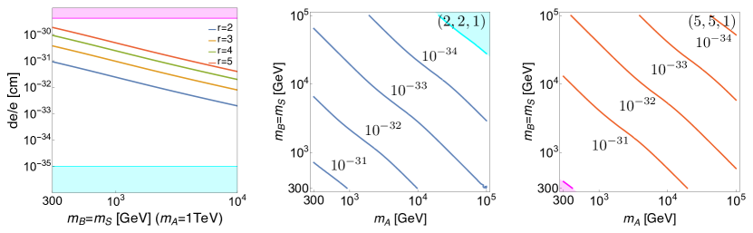
(a) Under the assumption of $m_{B}=m_{S}$.

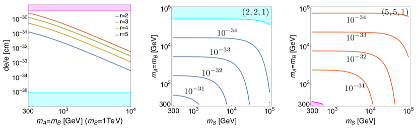
(b) Under the assumption of $m_{A}=m_{B}$.

Figure 3: Electron EDM induced by the Yukawa coupling of the $(r,r,1)$ SU(2)_L multiplets. Here, $\operatorname{Im}(sa^{*})=0.25$ is taken. In the upper (lower) panels, $m_{B}=m_{S}$ ($m_{A}=m_{B}$) is assumed. In the left panels, the four color lines illustrate each SU(2)_L representation, where $r=2,3,4,5$, respectively. The SU(2)_L representations in the middle and right panels are shown inside of the figures. The magenta bands denote the experimental bound on the electron EDM $|d_{e}^{\rm exp.}|<4.1\times 10^{-30}e\,{\rm cm}$ Roussy:2022cmp , and the cyan-shaded regions can not be probed due to the CKM contribution through the $e$–$N$ four-fermion interaction Ema:2022yra .

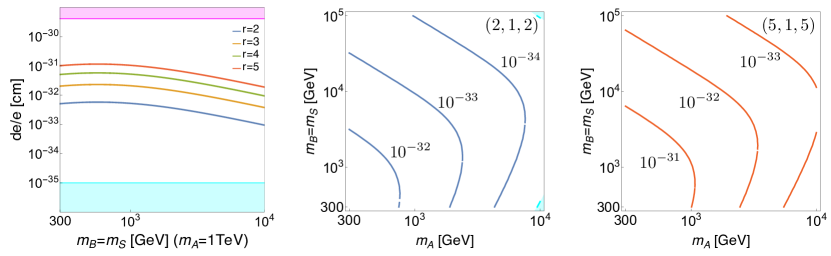
(a) Under the assumption of $m_{B}=m_{S}$.

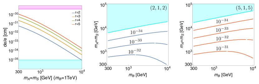
(b) Under the assumption of $m_{A}=m_{S}$.

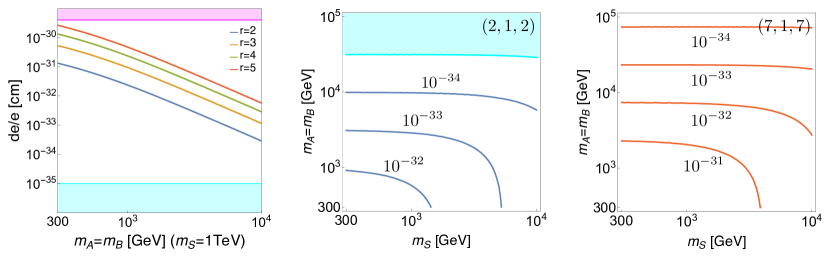
(c) Under the assumption of $m_{A}=m_{B}$.

Figure 4: Electron EDM induced by the Yukawa coupling of the $(r,1,r)$ SU(2)_L multiplets. In the upper, middle, lower panels, $m_{B}=m_{S}$ $m_{A}=m_{S}$, $m_{A}=m_{B}$ are assumed, respectively. The others are the same as in Fig. 3.

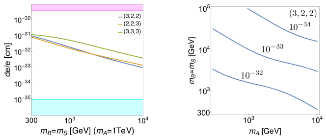
(a) Under the assumption of $m_{B}=m_{S}$.

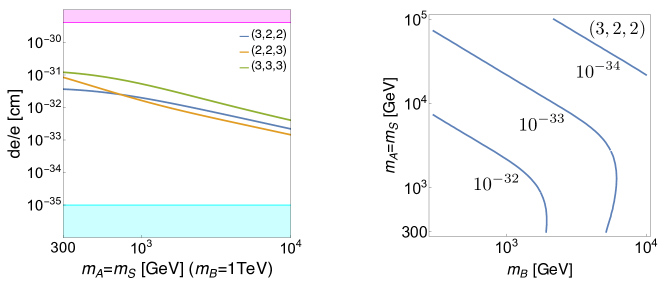
(b) Under the assumption of $m_{A}=m_{S}$.

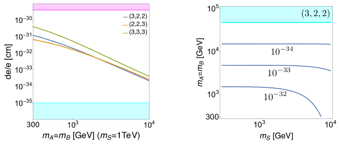
(c) Under the assumption of $m_{A}=m_{B}$.

Figure 5: Electron EDMs induced by the electroweak Weinberg operator, under the assumption that the SU(2)_L representations are $(A,B,S)=(3,2,2)$, $(2,2,3)$ and $(3,3,3)$. The others are the same as in Fig. 3.

4.2   $S=H$

Next, we discuss the importance of the electroweak Weinberg operator contribution in the case that the scalar $S$ is identified with the SM Higgs, and it has the CP-violating Yukawa couplings with $\psi_{A}$ and $\psi_{B}$. In this case, the two-loop Barr-Zee diagram is the dominant contribution to the electron EDM. The radiative correction to the contribution might be comparable to that from the electroweak Weinberg operator, both of which are three-loop level contributions. We will clarify this point first before showing the numerical results.

Let us assume $m_{S}(=m_{H})\ll m_{A}<m_{B}$. Integrating out $\psi_{B}$ at tree level generates the dimension-five operator of the Higgs boson and $\psi_{A}$, and then integrating out $\psi_{A}$ at one-loop level induces the effective operator $|H|^{2}F^{\mu\nu}\widetilde{F}_{\mu\nu}$. The coefficient is suppressed by $1/(m_{A}m_{B})$. The electron EDM is induced by another loop diagram with the effective operator. As a result, the electron EDM is proportional to $m_{e}/(m_{A}m_{B})$ with a two-loop factor. This means the electroweak Weinberg operator contribution has a similar mass parameter dependence to the Barr-Zee contribution. In Ref. Kuramoto:2019yvj , the anomalous dimensions for the dimension-five operator of the Higgs boson are evaluated at one-loop level. The corrections to the electron EDM from the anomalous dimensions might be comparable to the contribution from the electroweak Weinberg operator.

For concreteness, we assume $(A,B,S)=(3,2,2^{H})$, where $2^{H}$ means the SM Higgs boson. The Wilson coefficients $C_{W}$ for the electroweak Weinberg operator is approximately given as

$$\begin{aligned} C_{W}&\simeq\left\{\begin{aligned} &\frac{1}{(4\pi)^{4}}\mathop{\mathrm{Im}}(sa^{*})\times\frac{m_{A}}{8m_{B}^{3}}\left(11+8\ln\frac{m^{2}_{A}}{m^{2}_{B}}\right)\quad&(m_{H}\ll m_{A}<m_{B})\,,\\ &\frac{1}{(4\pi)^{4}}\mathop{\mathrm{Im}}(sa^{*})\times\frac{-5}{8m_{A}m_{B}}\quad&(m_{H}\ll m_{B}<m_{A})\,.\end{aligned}\right.\end{aligned}$$ (4.13)

Here, we take the triplet fermion $\psi_{A}$ with the Majorana mass $m_{A}$ and the doublet fermion $\psi_{B}$ with Dirac mass $m_{B}$. When $m_{B}<m_{A}$, $C_{W}$ is proportional to $1/(m_{A}m_{B})$. On the other hand, when $m_{A}<m_{B}$, it is suppressed by $m_{A}/m_{B}^{3}$. It comes from accidental cancellation between the leading contributions of $g_{1}$ and $g_{2}$ in $C_{W}$ in a limit of $m_{H}\rightarrow 0.$ Thus, the contribution to the electron EDM is more suppressed in the latter case.

Now we take a ratio between the contributions from the electroweak Weinberg operator ($d_{e}^{(W)}$) and from the correction to the Barr-Zee diagrams (${\delta d_{e}^{(BZ)}}$). It is approximately given as

$$\frac{d_{e}^{(W)}}{\delta d_{e}^{(BZ)}} \simeq\left\{\begin{aligned} &\frac{1}{64}\frac{\alpha^{2}_{2}}{\alpha_{e}}\left(\bar{\gamma}^{(3,0)}_{ss}\ln\frac{m_{B}}{m_{A}}\right)^{-1}\frac{m^{2}_{A}}{m_{B}^{2}}\frac{11+8\ln\frac{m^{2}_{A}}{m^{2}_{B}}}{2+\ln\frac{m^{2}_{A}}{m_{H}^{2}}}\quad&(m_{H}\ll m_{A}<m_{B})\,,\\ &\frac{5}{16}\frac{\alpha^{2}_{2}}{\alpha_{e}}\left[\left(3\bar{\gamma}^{(2,1/2)}_{ss}+\bar{\gamma}^{(2,1/2)}_{tt}\right)\ln\frac{m_{A}}{m_{B}}\right]^{-1}\frac{1}{2+\ln\frac{m^{2}_{B}}{m_{H}^{2}}}\quad&(m_{H}\ll m_{B}<m_{A})\,,\end{aligned}\right.$$ (4.14)

where $\bar{\gamma}^{(r,Y_{r})}_{ij}/(4\pi)\;(i,j=s,t)$ are anomalous dimension matrix components for the dimension-five operators of $\psi\psi H^{2}$ for the Barr-Zee diagrams. They depend on the gauge charges of the lighter fermion and are given as Bishara:2018vix ; Kuramoto:2019yvj

$$\bar{\gamma}^{(r,Y_{r})}_{ss} =-\left[6\alpha_{2}\left(C_{2}(r)+\frac{3}{4}\right)+6\alpha_{Y}\left(Y_{r}^{2}+\frac{1}{4}\right)-3\lambda^{\prime}-6\alpha_{t}\right]\,,$$ (4.15)

$$\bar{\gamma}^{(r,Y_{r})}_{tt} =-\left[6\alpha_{2}\left(C_{2}(r)-\frac{1}{4}\right)+6\alpha_{Y}\left(Y_{r}^{2}+\frac{1}{4}\right)-\lambda^{\prime}-6\alpha_{t}\right]\,,$$ (4.16)

where $\alpha_{2},\alpha_{Y},\alpha_{t}$ are for SU(2)_L, U(1)_Y and top-Yukawa coupling constants, respectively, and $\lambda^{\prime}(=\lambda/4\pi)$ is for the SM Higgs quartic coupling constant ($\lambda$). $C_{2}(r)$ and $Y_{r}$ are the Casimir operator and the hypercharge for the lighter fermion. ($C_{2}=2$ and $Y_{r}=0$ for $\psi_{A}$ and $C_{2}=3/4$ and $Y_{r}=1/2$ for $\psi_{B}$.)

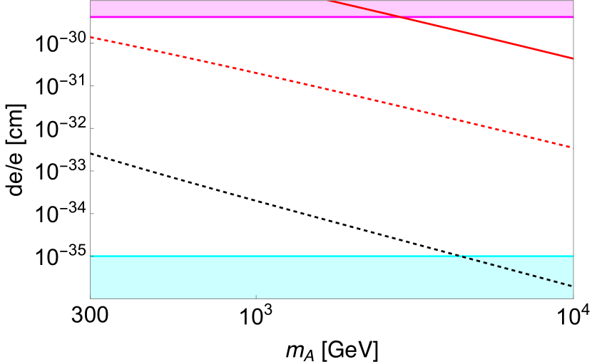
(a) $m_{B}=10m_{A}$

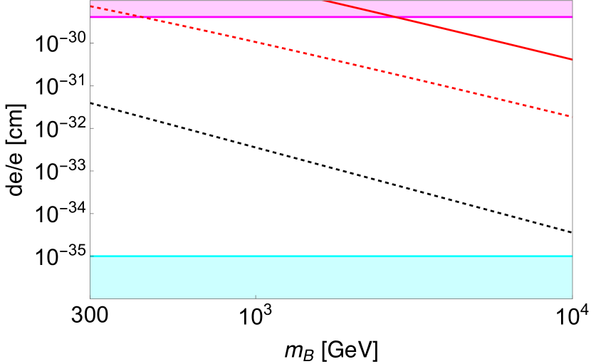
(b) $m_{A}=10m_{B}$

Figure 6: Contributions to the electron EDM from the electroweak Weinberg operator (dotted-black lines) and the radiative correction in the Barr-Zee diagrams (the dotted-red lines). The red-solid lines are for the sum of LO and NLO contributions in the Barr-Zee diagrams. We assume $(A,B,S)=(3,2,2^{H})$ ($2^{H}$ stands for the SM Higgs). In the left (right) panel, the triplet Majorana fermion (doublet Dirac fermion) is 10 times lighter than the doublet (triplet) one. $\operatorname{Im}(sa^{*})=0.25$ is taken.

As expected, the ratio in Eq. (4.14) is not suppressed by the power of the coupling constants. It is suppressed by $m^{2}_{A}/m^{2}_{B}$ in the case of $m_{A}<m_{B}$, while it is not in $m_{A}>m_{B}$. However, we find that the ratio is suppressed numerically. In Fig. 6, we show the contributions to the electron EDM from the correction to the Barr-Zee diagrams (${\delta d_{e}^{(BZ)}}$, the dotted red lines) and from the electroweak Weinberg operator ($d_{e}^{(W)}$, the dotted black lines), and the Barr-Zee diagram contribution including the correction (the red solid line). The Figs. 6(a) and  6(b) correspond to the cases of $m_{A}<m_{B}$ and $m_{B}<m_{A}$, respectively. Here, the heavier fermion mass is taken to be 10 times larger than the lighter one ($m_{B}=10m_{A}$ or $m_{A}=10m_{B}$). We take $m_{t}=172.57\;\rm GeV$, and $\alpha_{Y}=\alpha_{2}\tan^{2}\theta_{w}=0.01$ PDG:2024 as input parameters. We found that $d_{e}^{(W)}/{\delta d_{e}^{(BZ)}}$ is $1.0\times 10^{-3}\;(3.4\times 10^{-3})$ for $m_{A}<m_{B}$ ($m_{B}<m_{A}$) when the lighter fermion mass is 1 TeV.

5   Conclusions

The progress of the electron EDM measurements has been remarkable. The CP-violating interactions induced by BSM around the TeV scale have been constrained even if the electron EDM is generated at two-loop level. In the coming decades, experimental improvements are expected to probe the contributions even at three-loop level.

In this paper, we study the electron EDM generated by the electroweak Weinberg operator at three-loop level. If the CP-violating Yukawa couplings are introduced with SU(2)_L BSM multiplets, the electroweak Weinberg operator is generated at two-loop level. Below the electroweak scale, the electron EDM is radiatively induced at three-loop level since it is generated by another one-loop diagram with the electroweak Weinberg operator interaction. We introduce the SU(2)_L multiplets with TeV scale masses, which could be motivated by the dark matter multiplets, and investigated the predicted size of the electron EDM. It is found that the prediction would be covered by the future electron EDM measurements and might discover them since it may be larger than the SM contributions to the paramagnetic atom or molecule EDMs, $d_{e}^{\rm eq}=1.0\times 10^{-35}e$ cm. We notice that if large SU(2)_L multiplets, such as five- or seven-dimensional multiplets, are introduced, the electron EDM is enhanced by the cubic power of the dimension. Such large-dimensional multiplets are motivated in the minimal dark matter models due to the stability of dark matter.

We also discuss the relation between the Barr-Zee diagram and the electroweak Weinberg operator contributions to the electron EDM. If the SM Higgs has CP-violating Yukawa coupling with the SU(2)_L BSM multiplets, the Barr-Zee diagrams at two-loop level contribute to the electron EDM. Thus, the radiative correction to the Barr-Zee diagrams might be comparable to the contribution from the electroweak Weinberg operator. We compute the radiative correction to the Barr-Zee diagrams using the anomalous dimensions for the dimension-five operators of the SM Higgs and the fermion generated by integration of the heavier fermion, and compare it with that from the electroweak Weinberg operator contribution. We find the electroweak Weinberg operator contribution is numerically smaller than the radiative correction to the Barr-Zee diagrams and it can be safely negligible.

- (1) J. J. Hudson, et al., “Improved measurement of the shape of the electron,” Nature 473 (2011) 493–496.
- (2) ACME Collaboration, “Order of Magnitude Smaller Limit on the Electric Dipole Moment of the Electron,” Science 343 (2014) 269–272 [arXiv:1310.7534].
- (3) ACME Collaboration, “Improved limit on the electric dipole moment of the electron,” Nature 562 (2018) 355–360.
- (4) T. S. Roussy et al., “An improved bound on the electron’s electric dipole moment,” Science 381 (2023) adg4084 [arXiv:2212.11841].
- (5) R. Alarcon et al., “Electric dipole moments and the search for new physics,” in Snowmass 2021. 2022. arXiv:2203.08103.
- (6) T2K Collaboration, “Constraint on the matter–antimatter symmetry-violating phase in neutrino oscillations,” Nature 580 (2020) 339–344 [arXiv:1910.03887]. [Erratum: Nature 583, E16 (2020)].
- (7) T2K Collaboration, “Measurements of neutrino oscillation parameters from the T2K experiment using protons on target,” Eur. Phys. J. C 83 (2023) 782 [arXiv:2303.03222].
- (8) NOvA Collaboration, “Expanding neutrino oscillation parameter measurements in NOvA using a Bayesian approach,” Phys. Rev. D 110 (2024) 012005 [arXiv:2311.07835].
- (9) S. M. Barr and A. Zee, “Electric Dipole Moment of the Electron and of the Neutron,” Phys. Rev. Lett. 65 (1990) 21–24. [Erratum: Phys.Rev.Lett. 65, 2920 (1990)].
- (10) M. Cirelli, N. Fornengo, and A. Strumia, “Minimal dark matter,” Nucl. Phys. B 753 (2006) 178–194 [hep-ph/0512090].
- (11) J. Hisano, S. Matsumoto, M. Nagai, O. Saito, and M. Senami, “Non-perturbative effect on thermal relic abundance of dark matter,” Phys. Lett. B 646 (2007) 34–38 [hep-ph/0610249].
- (12) M. Cirelli, A. Strumia, and M. Tamburini, “Cosmology and Astrophysics of Minimal Dark Matter,” Nucl. Phys. B 787 (2007) 152–175 [arXiv:0706.4071].
- (13) M. Cirelli and A. Strumia, “Minimal Dark Matter: Model and results,” New J. Phys. 11 (2009) 105005 [arXiv:0903.3381].
- (14) J. Hisano, D. Kobayashi, N. Mori, and E. Senaha, “Effective Interaction of Electroweak-Interacting Dark Matter with Higgs Boson and Its Phenomenology,” Phys. Lett. B 742 (2015) 80–85 [arXiv:1410.3569].
- (15) N. Nagata and S. Shirai, “Higgsino Dark Matter in High-Scale Supersymmetry,” JHEP 01 (2015) 029 [arXiv:1410.4549].
- (16) CMS Collaboration, “Measurement of the W Production Cross Section in Proton-Proton Collisions at =13 TeV and Constraints on Effective Field Theory Coefficients,” Phys. Rev. Lett. 126 (2021) 252002 [arXiv:2102.02283].
- (17) K. Hagiwara, R. D. Peccei, D. Zeppenfeld, and K. Hikasa, “Probing the Weak Boson Sector in ,” Nucl. Phys. B 282 (1987) 253–307.
- (18) F. Boudjema, K. Hagiwara, C. Hamzaoui, and K. Numata, “Anomalous moments of quarks and leptons from nonstandard W W gamma couplings,” Phys. Rev. D 43 (1991) 2223–2232.
- (19) Y. Ema, T. Gao, and M. Pospelov, “Standard Model Prediction for Paramagnetic Electric Dipole Moments,” Phys. Rev. Lett. 129 (2022) 231801 [arXiv:2202.10524].
- (20) T. Abe, J. Hisano, and R. Nagai, “Model independent evaluation of the Wilson coefficient of the Weinberg operator in QCD,” JHEP 03 (2018) 175 [arXiv:1712.09503]. [Erratum: JHEP 09, 020 (2018)].
- (21) W. Kuramoto, T. Kuwahara, and R. Nagai, “Renormalization Effects on Electric Dipole Moments in Electroweakly Interacting Massive Particle Models,” Phys. Rev. D 99 (2019) 095024 [arXiv:1902.05360].
- (22) V. Fock, “Proper time in classical and quantum mechanics,” Phys. Z. Sowjetunion 12 (1937) 404–425.
- (23) J. S. Schwinger, “On gauge invariance and vacuum polarization,” Phys. Rev. 82 (1951) 664–679.
- (24) A. Schwarz, V. Fateev, and Y. Tyupkin, “On the particle-like solutions in the presence of fermions,” 155, Lebedev Institute, 1976.
- (25) C. Cronstrom, “A simple and complete Lorentz-covariant gauge condition,” Phys. Lett. B 90 (1980) 267–269.
- (26) M. A. Shifman, “Wilson Loop in Vacuum Fields,” Nucl. Phys. B 173 (1980) 13–31.
- (27) M. S. Dubovikov and A. V. Smilga, “Analytical Properties of the Quark Polarization Operator in an External Selfdual Field,” Nucl. Phys. B 185 (1981) 109–132.
- (28) V. A. Novikov, M. A. Shifman, A. I. Vainshtein, and V. I. Zakharov, “Calculations in External Fields in Quantum Chromodynamics. Technical Review,” Fortsch. Phys. 32 (1984) 585.
- (29) C. Ford, I. Jack, and D. R. T. Jones, “The Standard model effective potential at two loops,” Nucl. Phys. B 387 (1992) 373–390 [hep-ph/0111190]. [Erratum: Nucl.Phys.B 504, 551–552 (1997)].
- (30) J. R. Espinosa and R.-J. Zhang, “Complete two loop dominant corrections to the mass of the lightest CP even Higgs boson in the minimal supersymmetric standard model,” Nucl. Phys. B 586 (2000) 3–38 [hep-ph/0003246].
- (31) S. P. Martin, “Two Loop Effective Potential for a General Renormalizable Theory and Softly Broken Supersymmetry,” Phys. Rev. D 65 (2002) 116003 [hep-ph/0111209].
- (32) J. Hisano, T. Kitahara, N. Osamura, and A. Yamada, “Novel loop-diagrammatic approach to QCD parameter and application to the left-right model,” JHEP 03 (2023) 150 [arXiv:2301.13405].
- (33) T. Banno, J. Hisano, T. Kitahara, and N. Osamura, “Closer look at the matching condition for radiative QCD parameter,” JHEP 02 (2024) 195 [arXiv:2311.07817].
- (34) J. Hisano, K. Tsumura, and M. J. S. Yang, “QCD Corrections to Neutron Electric Dipole Moment from Dimension-six Four-Quark Operators,” Phys. Lett. B 713 (2012) 473–480 [arXiv:1205.2212].
- (35) F. Hoogeveen, “A bound on CP violating couplings of the W boson.”. MPI-PAE/PTh-25/87, 1987.
- (36) D. Atwood, C. P. Burgess, C. Hamazaou, B. Irwin, and J. A. Robinson, “One loop P and T odd W+- electromagnetic moments,” Phys. Rev. D 42 (1990) 3770–3777.
- (37) A. De Rujula, M. B. Gavela, O. Pene, and F. J. Vegas, “Signets of CP violation,” Nucl. Phys. B 357 (1991) 311–356.
- (38) H. Novales-Sanchez and J. J. Toscano, “Effective Lagrangian approach to fermion electric dipole moments induced by a CP-violating WW gamma vertex,” Phys. Rev. D 77 (2008) 015011 [arXiv:0712.2008].
- (39) B. Gripaios and D. Sutherland, “Searches for -violating dimension-6 electroweak gauge boson operators,” Phys. Rev. D 89 (2014) 076004 [arXiv:1309.7822].
- (40) Particle Data Group Collaboration, “Review of Particle Physics,” Phys. Rev. D 110 (2024) 030001.
- (41) F. Bishara, J. Brod, B. Grinstein, and J. Zupan, “Renormalization Group Effects in Dark Matter Interactions,” JHEP 03 (2020) 089 [arXiv:1809.03506].