Gravitational Wave Emission from Cosmic String Loops, II: Local Case

Abstract

Using lattice field simulations of the Abelian-Higgs model, we characterize the simultaneous emission of (scalar and gauge) particles and gravitational waves (GWs) by local string loops. We use network loops created in a phase transition, and artificial loops formed by either crossing straight-boosted or curved-static infinite strings. Loops decay via both particle and GW emission, on time scales $\Delta t_{\rm dec}\propto L^{p}$, where $L$ is the loop length. For particle production, we find $p\simeq 2$ for artificial loops and $p\lesssim 1$ for network loops, whilst for GW emission, we find $p\simeq 1$ for all loops. We find that below a critical length, artificial loops decay primarily through particle production, whilst for larger loops GW emission dominates. However, for network loops, which represent more realistic configurations, particle emission always dominates, as supported by our data with length-to-core ratios up to $L/r_{\text{c}}\lesssim 3500$. Our results indicate that the GW background from a local string network should be greatly suppressed compared to estimations that ignore particle emission.

Motivation.– It is nearly half a century since cosmic strings were introduced by Tom Kibble [1]. These are topologically stable line-like configurations, consisting of a network of ‘long’ strings, stretching across the horizon, and loops. The long-string density decreases as they intercommute forming loops, which in turn eventually decay. However, the dominant decay route of the loops has been a matter of debate since Kibble’s pioneering paper.

In the Nambu-Goto (NG) approximation of infinitely thin strings, the loops decay solely into gravitational waves (GWs), leading to a GW background (GWB) [2, 3, 4] potentially observable [5, 6, 7, 8, 9], depending on the string tension $\mu$. In reality, cosmic strings arise out of a phase transition involving a scalar-gauge sector, and hence a separate decay route opens up, as loops may decay into the fields they are made of [10, 11]. While this was a moot point in the past, given the string’s negligible contribution to Cosmic Microwave Background (CMB) anisotropies [12, 13, 14, 15, 16, 17], the situation has now changed in the present era of GW astronomy.

Pulsar timing array (PTA) collaborations have announced the first evidence for a GWB around $\sim\text{nHz}$ frequencies [18, 19, 20, 21]. While cosmic strings are possible sources of such observations, their contribution depends sensitively on the type of decay strings experience: is it primarily through GWs, or via particle production? For example, fitting PTA data to NG cosmic strings that only emit GWs leads to the tight constraint $G\mu\lesssim 10^{-10}$ [22, 23, 24], with $G$ Newton’s constant, whilst fitting to a field theory network that allows for particle production, loosens the constraint to $G\mu\lesssim 10^{-7}$ [25].

Revisiting the question of the dominant decay channel of local cosmic strings seems in order. With this in mind, [26] set up and evolved Abelian-Higgs loops, comparing the observed particle production with the traditional GW result from NG loops. For loops below a critical length, they found decay primarily through particle production, whilst for larger loops, GW emission dominates.

In this Letter, we extend the approach of [26], with two important differences: $i)$ we allow for the simultaneous emission of GWs and particles, as a true comparison requires, and $ii)$ besides artificially constructed ‘squared’ loops as in [26], we use another type of artificial loops following [11], as well as more realistic loops from lattice-simulated networks as in [10, 11]. We extend in this way to local cosmic string loops our previous study for global string loops [27]. Our key findings, discussed below, include a result similar to [26] with regard the existence of a critical length for artificial loops. However, the decay of loops originating from networks is found to be always dominated by particle emission. This implies that calculations ignoring particle production overestimate the amount of GW emitted, overconstraining $G\mu$.

Figure 1: Panel (A): Evolution of $\tilde{L}$ of a network loop (green), artificial loops of type I (red and blue) and type II (magenta). Here $\tau=0$ signals the moment when an isolated loop is left in the simulation. Solid lines for artificial loops represent a fit to an oscillation-averaged length, $\tilde{L}_{\rm av}$, and the dashed line an extrapolation of the previous fit to $\tau_{\text{dec}}$. Panel (B): $\Delta\tau_{\rm dec}$ vs $\tilde{L}_{0}$ for network loops, varying $N$ and $\ell_{\rm str}$, with blue and red shaded regions corresponding to linear and power-law fits, respectively. Panel (C): $\Delta\tau_{\rm dec}/\tilde{L}_{\text{av,0}}$ vs $\tilde{L}_{\text{av,0}}$ for artificial loops, with dashed, solid and dotted lines, representing power-law fits.

Model and loop configurations.– We consider an Abelian-Higgs model with a complex scalar field, $\varphi=(\phi_{1}+i\phi_{2})/\sqrt{2}$, and a U(1) gauge field, $A_{\mu}$, with lagrangian density $\mathcal{L}=-[(D_{\mu}\varphi)(D^{\mu}\varphi)^{*}+\frac{1}{4}F_{\mu\nu}F^{\mu\nu}+V(\varphi)]$, with $D_{\mu}=\partial_{\mu}-ieA_{\mu}$, $F_{\mu\nu}=\partial_{\mu}A_{\nu}-\partial_{\nu}A_{\mu}$, $V(\varphi)=\lambda(\varphi^{*}\varphi-v^{2}/2)^{2}$, $e$ the gauge coupling, and $\lambda$ and $v$ the self-coupling and vacuum expectation value (vev) of $\varphi$. After a phase transition from $\langle\varphi\rangle=0$ (symmetric phase) to $\langle|\varphi|^{2}\rangle=v^{2}/2$ (broken phase), cosmic strings arise as line-like configurations with energy-core widths set by the inverse masses of the resulting scalar and gauge particles at low energies, $r_{\text{s}}\sim 1/m_{\text{s}}$ and $r_{\text{g}}\sim 1/m_{\text{g}}$, where $m_{\text{s}}=\sqrt{2\lambda}v$ and $m_{\text{g}}=ev$. Upper bounds on the vev are set by CMB searches [12, 13, 14, 15, 16, 17] on cosmic strings as $v\lesssim 4.3\cdot 10^{15}$ GeV, and from PTA searches [22, 23, 24], assuming NG and $\mu=\pi v^{2}$, as $v\lesssim 6.9\cdot 10^{13}$ GeV. In this work, we set $e^{2}/\lambda=2$, and study two loop families:

$\bullet$ Network loops, obtained from the evolution of string networks created after simulating a phase transition. Following [11], simulations are initialized as a random Gaussian realization of $\varphi$, with a correlation length $\ell_{\rm str}$, that controls the initial string density. After diffusing the starting configuration, networks are evolved in radiation-domination (RD), where an initial extra-fattening phase is applied during one half-box light-crossing time. Afterwards, the network is evolved in Minkowski. In some of these simulations we end up with a single loop, which we use as our object of study, in isolation, until it collapses.

$\bullet$ Artificial loops, obtained from two procedures. Type I loops are generated from the intersection of two pairs of boosted infinite parallel strings, following [26]. The infinite static strings are built using Nielsen-Olsen vortex solutions at different orientations, and then boosted. When the strings intersect, they form a pair of ‘squared’ loops. Type II loops are generated following [10, 11], by setting gauge field links generating a net magnetic flux ($\pm 2\pi$) on the plaquettes pierced by the string. After a diffusive phase, this allows the creation of static strings with arbitrary shapes. Our initial configuration is composed of four curved strings that intersect soon after evolution begins, creating two non-squared loops. In both procedures, we wait for one loop to disappear and study the other in isolation, until it collapses.

For further details on how loops are generated, see the supplemental material [28]. We determine the length of a loop, $L$, by identifying pierced plaquettes in a gauge-invariant manner [29, 10], accounting for the Manhattan effect [30, 31, 32]. We also measure the energy of strings as

$$E_{\text{str}}=\int\text{d}^{3}x\,W(\varphi)\Big{[}|\dot{\varphi}|^{2}+|\vec{D}\varphi|^{2}+\frac{\vec{E}^{2}}{2}+\frac{\vec{B}^{2}}{2}+V(\varphi)\Big{]},$$

where $E_{i}=F_{0i}$ and $B_{i}=\varepsilon_{ijk}F^{jk}/2$ are the electric and magnetic fields, and $W(\varphi)=[V(\varphi)/W_{0}]\cdot\Theta(v^{2}/2-|\varphi|^{2})$ is a weight function that only selects regions occupied by strings, with $W_{0}=\lambda v^{4}/4$ and $\Theta(x)$ the step function.

We have used $\mathcal{C}$osmo$\mathcal{L}$attice [33, 34, 35] to evolve the dynamics of the scalar-gauge field system and the GWs [36, 37] in regular periodic lattices. From now on, we express observables in terms of dimensionless variables: $\tilde{\varphi}=\varphi/v$, $\tilde{L}=\sqrt{\lambda}v\,L$, $\tau=\sqrt{\lambda}v\,t$, ${\tilde{E}}_{\text{str}}=(\sqrt{\lambda}/v)\,E_{\text{str}}$, and for the (comoving) momentum, $\kappa=k/\sqrt{\lambda}v$.

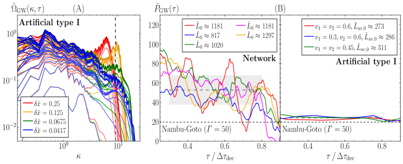
Figure 2: Panel (A): Evolution of $\tilde{\Omega}_{\rm GW}(\kappa,\tau)$ for artificial type I loops with varying UV resolution, $\delta\tilde{x}$, but fixed lattice size. The dashed vertical line indicates the scale of the string width, $\kappa_{\text{c}}=2\pi/\tilde{r}_{\text{c}}$. Spectra go from early to late times from bottom to top, with lines plot every $\Delta\tau=4$ units. Panel (B): Power emission of GWs of network (left) and type I artificial (right) loops.

Results on loop decay.– We have studied 48 network loops, 14 artificial loops of type I, and 6 of type II, with initial length-to-core width ratios $850\lesssim L_{0}/r_{\text{c}}\lesssim 3500$ (network) and $120\lesssim L_{0}/r_{\text{c}}\lesssim 640$ (artificial). We have characterized the dependence of the decay time of loops $\Delta\tau_{\text{dec}}$, on their initial length $\tilde{L}_{0}$, and energy $\tilde{E}_{\text{str,0}}$. For details on the simulations, see [28].

Fig. 1-(A) shows the length evolution of representative loops. The length of a network loop (in green) decays rapidly in time, with no oscillations. Artificial loops, however, live much longer and oscillate many times before decaying. In the case of type I loops, depending on the boost velocities ($v_{1},\,v_{2}$), the loop either disappears smoothly (in red), or it disappears abruptly (in blue) due to a “double-line collapse” (dLC), when two parallel segments approach each other and annihilate. Type II loops display a similar decay pattern (in magenta). As dLC is a result of the artificial initial condition, we remove its effect on our results for artificial loops by performing a 3-parameter fit to an oscillation-averaged length $\tilde{L}_{\text{av}}(\tau)=C(\tau_{\text{dec}}-\tau)^{p}$ [11] (solid lines, with $p\approx 1/2$). This allows to determine: $i)$ $\Delta\tau_{\text{dec}}=\tau_{\text{dec}}-\tau_{0}$ as the lifetime, with $\tau_{0}$ the time when the loop becomes isolated in the simulation, and $ii)$ the initial (oscillation-averaged) length of the isolated loop, $\tilde{L}_{{\rm av},0}=\tilde{L}_{\text{av}}(\tau_{0})$. A similar behaviour is observed fitting against the loops’ energy as $\tilde{E}_{\text{av}}=D(\tau_{\text{dec}}-\tau)^{q}$, with $q\approx 1/2$, leading to an estimate of the (oscillation-averaged) initial string energy $\tilde{E}_{\text{av,0}}$.

Fig. 1-(B) shows $\Delta\tau_{\rm dec}$ vs $\tilde{L}_{0}$ for all network loops studied. As in [11, 27], we observe $\Delta\tau_{\rm dec}$ roughly scaling linearly with $\tilde{L}_{0}$. We quantify this by performing two different fits, a linear fit $\Delta\tau_{\text{\rm dec}}=c_{1}\tilde{L}_{0}+c_{2}$ (blue dashed line and band), and a power-law fit $\Delta\tau_{\rm dec}=A\tilde{L}_{0}^{\alpha}$ (red line and band). Both fits describe the data qualitatively well in the range of lengths studied. We obtain $(c_{1},\,c_{2})=(0.182\pm 0.013,\,69\pm 16)$ and $(A,\,\alpha)=(1.9\pm 0.7,\,0.71\pm 0.05)$. Similar linear and power-law fits are also obtained as $\Delta\tau_{\rm dec}=d_{1}\tilde{E}_{{\rm str},0}+d_{2}$ and $\Delta\tau_{\rm dec}=B\tilde{E}_{{\rm str},0}^{\beta}$, yielding $(d_{1},\,d_{2})=(0.097\pm 0.007,\,63\pm 18)$ and $(B,\,\beta)=(1.0\pm 0.5,\,0.73\pm 0.06)$. If the linear fit is assumed, we find a particle emission power $\tilde{P}_{\rm part}=\text{d}\tilde{E}_{\text{str}}/\text{d}\tau=10.3\pm 0.7$, independent of the loop length. If we use instead the power-law fit, we obtain $\tilde{P}_{\rm part}\propto\tilde{L}^{\gamma}$, with $\gamma=\alpha(1-\beta)/\beta=0.26\pm 0.08$, indicating that particle emission power increases weakly with the loops’ length. We note that $\gamma\neq 0$ (equivalently $\beta\neq 1$), which represents a deviation from a linear fit, might be a volume effect due to having loops with lengths much larger than the lattice box side. This requires further investigation.

Fig 1-(C) shows $\Delta\tau_{\rm dec}/\tilde{L}_{\text{av,0}}$ as a function of $\tilde{L}_{\text{av,0}}$ for artificial loops. Fitting data to a power law $\Delta\tau_{\text{dec}}=A\tilde{L}_{{\rm av},0}^{\alpha}$, yields $(A\cdot 10^{3},\,\alpha)=(21\pm 3,\,2.027\pm 0.025)$ (type I) and $(A\cdot 10^{3},\,\alpha)=(33\pm 12,\,1.97\pm 0.07)$ (type II). While this fit is valid for all type I loops studied, independently of $(v_{1},v_{2})$ and $\delta x$ (indicating small discretization effects), it does depend on whether dLC is removed. For example, without removal, we see that for the loops with $(v_{1},\,v_{2})=(0.3,0.6)$, setting the decay time at the moment of dLC, yields $(A\cdot 10^{3},\,\alpha)=(8.3\pm 1.6,\,2.16\pm 0.03)$ (see empty circles). Fitting the data as $\Delta\tau_{\text{dec}}=B\tilde{E}_{{\rm av},0}^{\beta}$, we obtain $(B\cdot 10^{3},\,\beta)=(5.4\pm 1.0,\,1.988\pm 0.026)$ (type I) and $(B\cdot 10^{3},\,\beta)=(3.4\pm 2.5,\,2.08\pm 0.13)$ (type II). Approximating $\alpha\approx\beta\approx 2$, implies a particle emission power as $\tilde{P}_{\rm part}=C/\tilde{L}$, with $C\equiv(2\sqrt{AB})^{-1}=47\pm 5$ (type I) and $C=47\pm 19$ (type II). Particle production for artificial loops is therefore suppressed the larger the loop.

Unlike global loops [27], the dynamics of local loops are very sensitive to ultraviolet (UV) effects. For example, generating the same type I loop configuration with different lattice spacing $\delta\tilde{x}$’s, leads to identical $\Delta\tau_{\rm dec}$ for $\delta\tilde{x}=0.0417$ and $\delta\tilde{x}=0.0625$, but underestimates it by $\sim 5,10,15$ and $40\%$ for $\delta\tilde{x}=0.125,0.1875,0.25,0.5$, respectively. As a compromise, we use $\delta\tilde{x}=0.1875$ in our study, guaranteeing $\lesssim 10$% systematic errors. For network loops, using a coarse-graining procedure as in [11], we observe that $\delta\tilde{x}=0.125$ leads to lifetimes only $\sim 5\%$ larger than for $\delta\tilde{x}=0.25$, so we used the latter.

Results on GW emission.– Tensor perturbations $h_{ij}$ that represent GWs ($\partial_{i}h_{ij}=h_{ii}=0$) emitted by loops are obtained by solving $\ddot{h}_{ij}-\vec{\nabla}^{2}h_{ij}=2m_{p}^{-2}\Pi_{ij}^{\rm TT}$, where $m_{\text{p}}\simeq 2.435\cdot 10^{18}$ GeV is the reduced Planck mass, $[\cdots]^{\rm TT}$ implies transverse-traceless projection, and $\Pi_{ij}\equiv 2{\rm Re}[(D_{i}\varphi)(D_{j}\varphi)^{*}]-E_{i}E_{j}-B_{i}B_{j}$. We obtain the (normalized) GW energy density spectrum as [38]

$$\Omega_{\rm GW}(k,t)\equiv{1\over\rho_{\rm t}}\frac{\text{d}\rho_{\rm GW}}{\text{d}\log k}=\frac{k^{3}m_{\text{p}}^{2}}{8\pi^{2}{\mathcal{V}}\rho_{\rm t}}\big{\langle}\dot{{h}}_{ij}(k,t)\dot{h}^{*}_{ij}(k,t)\big{\rangle}_{\hat{\Omega}_{k}},$$

where $\rho_{\rm t}$ is the total energy density of the scalar and gauge fields in a lattice of volume $\mathcal{V}$, and $\langle\cdots\rangle_{\hat{\Omega}_{k}}$ represents angular averaging in Fourier space. The total GW energy emitted by a loop is obtained via $E_{\text{GW}}(t)=\rho_{\rm t}{\mathcal{V}}\int\Omega_{\rm GW}(k,t)\,\text{d}\log k\,$, so that in program variables we write $\tilde{\Omega}_{\rm GW}(\kappa,\tau)=(v/m_{\text{p}})^{-2}\Omega_{\rm GW}(k,t)$ and $\tilde{E}_{\rm GW}=\sqrt{\lambda}\,(v/m_{\text{p}})^{-2}(E_{\rm GW}/v)$. For simplicity, we focus on the GW emission by network and artificial type I loops only.

Given the UV dependencies observed in the dynamics of local loops, we first need to quantify UV effects on their GW emission. In fig. 2-(A) we plot the evolution of the GW spectra emitted by a given artificial type I loop configuration, for several values of $\delta\tilde{x}$. We observe the presence of an infrared (IR) peak around $\kappa\sim 0.4-0.5$ for all resolutions. A second peak emerges at UV scales for large $\delta\tilde{x}$ (red and yellow spectra) close to the core radius scale, at $\kappa_{\text{c}}=2\sqrt{2}\pi$ (dashed vertical line). This UV peak is suppressed for finer lattices (green and blue spectra), signaling it is a lattice artifact. Overall, we observe that simulations with $\delta\tilde{x}\lesssim 0.1875$ agree up to scales $\kappa_{\text{cut}}\sim 2.5$ for type I loops, which justifies to compute $\tilde{E}_{\rm GW}$ integrating up to such cutoff. For network loops we also keep the same cutoff.

We determine the GW power emitted by network loops as a rolling average, with

$$P_{\rm GW}(t)\equiv\frac{\rho_{\rm t}{\mathcal{V}}}{2T}\int^{t+T}_{t-T}\text{d}t^{\prime}\int_{0}^{k_{\text{cut}}}\dot{\Omega}_{\text{GW}}(k,t^{\prime})\,\text{d}\log k\,,$$

which we plot in the left panel of fig. 2-(B) in terms of program variables, $\tilde{P}_{\rm GW}\equiv(P_{\rm GW}/v^{2})\,/\,(v/m_{\text{p}})^{2}$, as a function of the lifetime fraction of the loops $\tau/\Delta\tau_{\rm dec}$, for $\tilde{T}\equiv(\sqrt{\lambda}v)T=20$. We have checked that the results are insensitive to choosing larger values of $\tilde{T}$. The amplitude of $\tilde{P}_{\rm GW}$ is roughly constant, with fluctuations depending on the string evolution. Averaging on the range $\tau/\Delta\tau_{\text{dec}}\in[0.3,0.8]$, leads to $\tilde{P}_{\rm GW}=53\pm 15$, which is only $\sim 20\%$ of the value obtained for global network loops [27], but still $\sim 2-3$ times larger than the NG prediction (shown by the horizontal dashed black line, using $\mu=\pi v^{2}$ and $\mathit{\Gamma}=50$ [6]).

For type I artificial loops, a different approach is required to determine their GW power emission. This is because, due to their longer lifetimes (often dozens of times the half-box-light-crossing time of the lattice), previously emitted GWs can interfere with newly produced ones, leading e.g. to spectral oscillations in the late time GW spectra, see fig. 2-(A). To prevent this volume effect affecting the results, we set GWs to zero when the loop starts oscillating, and evolve the GWs normally until we measure the GW power spectrum after a time $\Delta T_{\text{GW}}$. We then reset GWs to zero and repeat the procedure until the loop decays. The averaged GW emission power during each sub-interval is computed as

$$P_{\text{GW}}(t)=\frac{\rho_{\text{t}}{\mathcal{V}}}{\Delta T_{\text{GW}}}\int_{0}^{k_{\text{cut}}}\Omega_{\text{GW}}(k,t)\,{\rm d}\log k\,.$$ (1)

We use $\Delta\tilde{T}_{\rm GW}=160$, which is sufficiently large to capture all relevant frequencies, but small enough to prevent finite-volume effects. We find that using $\Delta\tilde{T}_{\text{GW}}=80-200$ leads to less than $10$% discrepancies. We plot $\tilde{P}_{\rm GW}$ for artificial type I loops in the right panel of fig. 2-(B), as a function of the loops’ lifetime fraction, $\tau/\Delta\tau_{\rm dec}$. We find that the emission power remains mostly constant during the lifetime of the loops. Averaging on the range $\tau/\Delta\tau_{\text{dec}}\in[0.3,0.8]$ leads to $\tilde{P}_{\text{GW}}=24.2\pm 1.4$, slightly above the NG prediction for $\mu=\pi v^{2}$ and $\mathit{\Gamma}=50$.

Comparing GW and particle emission rates for artificial loops of type I, as obtained earlier, leads to

$${P_{\rm GW}\over P_{\rm part}}=\displaystyle{24.2\pm 1.4\over 66\pm 7}\left({v\over m_{\text{p}}}\right)^{2}\left({L\over r_{c}}\right)^{1+\delta}\,,$$ (2)

with $\delta=0.007\pm 0.018$. This implies that GW emission dominates ($P_{\rm GW}>P_{\rm part}$) for large loops with $L>L_{\rm crit}$, while particle production dominates ($P_{\rm part}>P_{\rm GW}$) for small loops with $L<L_{\rm crit}$, with $L_{\rm crit}$ a critical length. Neglecting the small correction $\delta$, so that $P_{\rm GW}/P_{\rm part}\propto L$, we find, from the condition $P_{\rm GW}(L_{\rm crit})=P_{\rm part}(L_{\rm crit})$,

$$L_{\text{crit}}\approx(2.8\pm 0.3)\,r_{\text{c}}\left(\frac{v}{m_{{}_{\mathrm{p}}}}\right)^{-2}\,,$$ (3)

with $r_{\text{c}}$ the string core radius. Using PTA constraints, $v\lesssim 3\cdot 10^{-5}m_{\text{p}}$, leads to a critical length at least as large as $L_{\rm crit}/r_{\text{c}}\gtrsim 10^{9}$. We confirm therefore the prediction in [26] on the existence of a critical length for type I artificial loops. We obtain however a value $\sim 10$ times larger, which we believe is quite precise, as it is based on a larger loop set and on measuring directly the GW emission from the loops on the lattice (as opposed to using NG predictions).

Similarly, for the network loops we obtain

$${P_{\rm GW}\over P_{\rm part}}=\left\{\begin{array}[]{ll}\displaystyle{53\pm 15\over 10.3\pm 0.7}\left({v\over m_{\text{p}}}\right)^{2}&\,,~{}~{}~{}{\rm linear~{}fit\vspace*{1mm}}\\ \displaystyle{53\pm 15\over 1.6\pm 1.0}\left({v\over m_{\text{p}}}\right)^{2}\left({L\over r_{\text{c}}}\right)^{-\gamma}&\,,~{}~{}~{}{\text{power-law fit}}\end{array}\right.$$ (6)

with $\gamma=0.26\pm 0.08$. This implies a ratio $P_{\rm GW}/P_{\rm part}$ which is either scale-invariant if a linear relation $\Delta\tau_{\rm dec}\propto\tilde{L}$ is assumed, or depends at most weakly on the loop length roughly as $\propto 1/{\tilde{L}}^{1/4}$, if a power-law fit $\Delta\tau_{\rm dec}\propto{\tilde{L}}^{\alpha}$ is assumed instead. Either way, this result implies that, contrary to artificial loops, particle emission dominates at all scales for network loops, as supported by our data with length-to-core width ratios up to $L/r_{\text{c}}\lesssim 3500$.

Discussion.– Cosmic string networks are predicted by a variety of field theory and superstring early universe scenarios [39, 40, 41, 42, 43, 44], and are expected to create a plethora of observational effects, from CMB anisotropies in the form of power spectra [12, 15, 16, 17, 45] and bispectra [46, 47, 48], to lensing events [49, 50], cosmic ray production [51, 52, 53, 54, 55, 56, 57, 58, 59, 60], and GW emission [2, 4, 61, 62, 63, 64, 65, 6, 7, 8, 66, 67, 68, 69, 70, 71, 72]. The relevance of particle production by string loops has been however under debate, since Kibble’s pioneering paper [1].

In this Letter we study the emission by local string loops of (scalar and gauge) particles and GWs, considering $i)$ artificial loops, obtained from the crossing of either straight-boosted (type I) or curved-static (type II) infinite strings, and $ii)$ network loops, obtained from the lattice simulation of string networks. We find that below a critical length, $L_{\rm crit}$, artificial loops decay primarily through particle production, whilst for larger loops GW emission dominates. This agrees with [26], which showed the existence of a critical length for type I artificial loops. We obtain however a value of $L_{\rm crit}$ which is $\sim 10$ times larger than in [26]. For network loops, on the contrary, we find that particle emission dominates for all loops studied, with length-to-core width ratios up to $L/r_{\text{c}}\lesssim 3500$. We observe no indication that this should change for longer loops. GW emission in this case, is suppressed compared to particle production as $P_{\rm GW}/P_{\rm part}\simeq 5\cdot(v/m_{p})^{2}\ll 1$. If we saturate the CMB bound $v\lesssim v_{\rm CMB}=10^{-3}m_{\text{p}}$, it is at most as large as $P_{\rm GW}/P_{\rm part}\lesssim 10^{-6}$, which justifies a posteriori that we neglected the backreaction of the GWs onto the loops.

Extrapolating our results to cosmological scales, we expect particle emission to reduce the number density of loops along cosmic history, resulting in a suppression of the GWB spectrum from a local string network:

$\bullet$ Considering artificial loops, the suppression should only affect the highest frequencies in the spectrum, as these are sourced by early produced loops, which will be small enough to verify $L<L_{\rm crit}$. This effect has ben quantified in [60, 73] using the value of $L_{\rm crit}$ from [26], showing a suppression in the high frequency tail of the GWB above a cutoff, which remains however outside the range of current and planned GW detectors. As our computation of $L_{\rm crit}$ yields a value $\sim 10$ times larger than in [26], we expect to reduce the frequency cut-off scale in the GWB, although not enough to make it observable.

$\bullet$ Considering network loops, we expect particle production to essentially suppress the GWB from a network of local strings at all frequencies. Assuming the linear fit to the decay of the loops, we obtain that loops will decay a factor $P_{\rm part}/P_{\rm GW}\sim 10^{6}\cdot(v/v_{\rm CMB})^{-2}$ faster than based solely on GW emission. This will reduce substantially the number of loops available at any moment in cosmic history, suppressing the GWB amplitude in the whole frequency range. We will present the details of this elsewhere. Here we simply anticipate that current constraints on GWB signals by PTA observations, will restore the compatibility of the data with energy scales associated to the string formation up to GUT scales, $v\sim 10^{-3}m_{\text{p}}$, similarly as in the CMB bound.

As a final remark, we highlight that network loops are precisely the type of loops expected from a scaling local string network generated after an early Universe phase transition, so they represent more realistic configurations than the artificial loops.

Supplemental material for the Letter:
Gravitational Wave Emission from Cosmic String Loops, II: Local Case

We have used the package $\mathcal{C}$osmo$\mathcal{L}$attice [33, 34, 35] to initialise and to evolve the dynamics of the scalar-gauge field system and of the GWs [36, 37] in regular lattices with periodic boundary conditions, with $N$ points/dimension. We denote the lattice spacing by $\delta x$, and the length of the side of a lattice box as $L_{\rm B}$.

Generation of network loops. Network loops are generated from the decay of string networks that are close to the scaling regime [74, 75, 76], following the procedure in [11]. They are expected to have shapes and features similar to loops from a realistic phase transition in the early universe. Simulations are initialized with a Gaussian random realization of the complex scalar field, $\varphi=(\phi_{1}+i\phi_{2})/\sqrt{2}$, in Fourier space, with power spectrum for each field component

$$\Delta_{\phi_{i}}(k)=\frac{k^{3}v^{2}\ell_{\text{str}}^{3}}{\sqrt{2\pi}}\exp\left(-\frac{1}{2}k^{2}\ell_{\text{str}}^{2}\right)\,.$$ (S1)

normalized so that $\langle\phi_{1}^{2}+\phi_{2}^{2}\rangle=v^{2}$, where $\langle\cdots\rangle$ denotes the expectation value. Here $\ell_{\text{str}}$ is a correlation length that controls the density of the resulting network. The gauge field and the time derivatives of both fields are set to zero.

The resulting field configuration is too energetic and contains no magnetic field. To get rid of the excess energy and allow the magnetic flux to form inside the strings, we evolve the configuration following diffusion equations of the form,

$$\begin{array}[]{rl}\sqrt{\lambda}v\dot{\varphi}-\partial_{i}\partial_{i}\varphi&=-\lambda(2|\varphi|^{2}-v^{2})\varphi\,,\\[10.0pt] \sqrt{\lambda}vF_{0i}-\partial_{j}F_{ji}&=2e\imaginary\left[\varphi^{*}D_{i}\varphi\right]\,,\end{array}$$ (S2)

where $\dot{f}=\text{d}f/\text{d}t$. The diffusive phase is applied for $\sqrt{\lambda}v\Delta t_{\rm diff}=20$ units, which we find to be enough for our purposes. An illustrative example of the resulting network is presented in the left panel of fig. S1.

aa

Figure S1: Three-dimensional snapshots of $|\varphi|^{2}=0.3v^{2}$ surfaces from a network simulation with $N=224$ and $\delta x=0.5/\sqrt{\lambda}v$, generated with ${\ell}_{\text{str}}=15/\sqrt{\lambda}v$. The snapshots correspond to the end of diffusion (left), the end of the extra-fattening phase (center), an instant when a single isolated loop is left (right).

After the diffusion process, we let the network evolve in a radiation-dominated (RD) background, with scale factor $a(\eta)=\eta/\eta_{0}$, where $\eta$ indicates the conformal time and $\eta_{0}=70/\sqrt{\lambda}v$ in our simulations. While it would be possible to obtain analogous results working in Minkowski background, as done in [11], evolving the network in RD dissipates some of the energy radiated from its decay. Moreover, we find the networks to decay slightly faster in an expanding background compared to a flat one.

Evolving strings in an expanding background leads to a loss of resolution of the string core. To prevent this from happening, we perform an initial phase of extra-fattening [77], in which the fields are evolved with equations of motion,

$$\begin{array}[]{rl}\displaystyle\varphi^{\prime\prime}+2\frac{a^{\prime}}{a}\varphi^{\prime}-D_{i}D_{i}\varphi&=\displaystyle-a^{-2}\lambda\left(2|\varphi|^{2}-v^{2}\right)\varphi\,,\\[10.0pt] \displaystyle\partial_{0}F_{0i}+4\frac{a^{\prime}}{a}F_{0i}-a^{-4}\partial_{j}F_{ji}&\displaystyle=2a^{-2}e\imaginary\left[\varphi^{*}D_{i}\varphi\right]\,,\end{array}$$ (S3)

where $f^{\prime}=\text{d}f/\text{d}\eta$. The extra-fattening phase is set to last for a total of $\Delta\eta_{\text{ef}}=\sqrt{\eta_{0}(\Delta\eta_{\text{HL}}+\eta_{0})}$, where $\Delta\eta_{\text{HL}}=L_{\rm B}/2$ is the half-box light-crossing time of the lattice, with $L_{\rm B}$ the side’s length of the lattice box. The central panel of fig. S1 shows an example of a network at the end of the extra-fattening phase.

After this phase, the fields are evolved physically in a RD background, with equations of motion

$$\begin{array}[]{rl}\displaystyle\varphi^{\prime\prime}+2\frac{a^{\prime}}{a}\varphi^{\prime}-D_{i}D^{i}\varphi_{i}&\displaystyle=-a^{2}\lambda\left(2|\varphi|^{2}-v^{2}\right)\varphi\,,\\[10.0pt] \displaystyle\partial_{0}F_{0i}-\partial_{j}F_{ji}&\displaystyle=2a^{2}e\imaginary[\varphi^{*}D_{i}\varphi]\,.\end{array}$$ (S4)

for an additional time $\Delta\eta_{\text{RD}}=\Delta\eta_{\text{HL}}-\Delta\eta_{\text{ef}}$. The initial extra-fattening phase ensures that, by the end of the physical evolution phase, the width of the string is equal to that at the end of diffusion.

By the end of the evolution in a RD background, the string network is close to the scaling regime. In most cases, however, the network has not yet decayed into a single loop. We subsequently evolve the resulting network in a Minkowski background so that it is able to decay. Note that, when changing from RD to Minkowski, it takes some time for the network to adapt to the new background, since the characteristics of the scaling regime depend on the background metric. After changing the metric, we wait for half a half-box light-crossing time, $\Delta t_{\text{HL}}/2$, before starting to study any isolated loop that may arise. We call this period a transient phase. We believe this minimizes the impact of the sudden change of background. The evolution in Minkowski background is held for a maximum time of $2\Delta t_{\text{HL}}$, including the transient phase, which we found enough to typically have one isolated string loop remaining. An example of an isolated network is presented in the right panel of fig. S1.

After the transient period, if an isolated loop is found we turn on the emission of GWs, and study the evolution of the loop until it disappears. Approximately, $\sim 20\%$ of our simulations lead to isolated loops, of which $\sim 80\%$ can be used for our study. We discard those loops that self intersect forming several loops of similar size or infinite strings. Altogether, only $\sim 16\%$ of the simulations are suitable for this work.

Generation of artificial loops of type I. Artificial loops of type I are generated from the intersection of two pairs of parallel infinite boosted strings, following the procedure used in [26], see also [27]. We choose the initial configuration so that one of the two loops resulting from the intersection of the infinite strings is much larger than the other one, and wait for the smaller one to decay before starting our study of the longer loop. We now describe the initialization procedure in detail. We consider one pair parallel to the $z$ axis and the other parallel to the $x$ axis, and we refer to each of them with subscripts “1” and “2”, respectively, which should not be confused with the component index of the gauge field, $\mu=0,1,2,3$.

We first explain how the pair of strings parallel to the $z$ axis is generated. The starting point is the solution for the NO vortex [78] in the temporal gauge, $\varphi^{(k)}_{\text{NO}}$ and $A^{(k)}_{\text{NO},\mu}$, where $k=\pm 1$ indicates the winding number of the string. The static NO configuration is boosted in the $(x,y)$-plane with velocity $\vec{v}_{1}=v_{1}(\sin\alpha_{1},\cos\alpha_{1})$, resulting in

$$\begin{array}[]{rl}\bar{\varphi}_{\vec{v}_{1}}^{(\pm)}(x,y;t)&=\varphi_{\text{NO}}^{(\pm)}(x^{\prime},y^{\prime})\,,\\[5.0pt] \bar{A}_{\vec{v}_{1},0}^{(\pm)}(x,y;t)&=-\gamma_{1}s_{1}v_{1}A_{\text{NO},1}^{(\pm)}(x^{\prime},y^{\prime})-\gamma_{1}c_{1}v_{1}A_{\text{NO},2}^{(\pm)}(x^{\prime},y^{\prime})\,,\\[5.0pt] \bar{A}_{\vec{v}_{1},1}^{(\pm)}(x,y;t)&=[1+(\gamma_{1}-1)s_{1}^{2}]A_{\text{NO},1}^{(\pm)}(x^{\prime},y^{\prime})+(\gamma_{1}-1)s_{1}c_{1}A_{\text{NO},2}^{(\pm)}(x^{\prime},y^{\prime})\,,\\[5.0pt] \bar{A}_{\vec{v}_{1},2}^{(\pm)}(x,y;t)&=(\gamma_{1}-1)s_{1}c_{1}A_{\text{NO},1}^{(\pm)}(x^{\prime},y^{\prime})+[1+(\gamma_{1}-1)c_{1}^{2}]A_{\text{NO},2}^{(\pm)}(x^{\prime},y^{\prime})\,,\end{array}$$ (S5)

where we define $s_{1}=\sin\alpha_{1}$, $c_{1}=\cos\alpha_{1}$ and $\gamma_{1}=(1-v_{1}^{2})^{1/2}$. Here $(x^{\prime},y^{\prime})$ are the coordinates in the rest frame of the string and $(t,x,y)$ are the coordinates in the boosted frame, related by

$$\begin{array}[]{rl}x^{\prime}&=-\gamma_{1}v_{1}s_{1}t+[1+(\gamma_{1}-1)s_{1}^{2}]x+(\gamma_{1}-1)s_{1}c_{1}y\,,\\[5.0pt] y^{\prime}&=-\gamma_{1}v_{1}c_{1}t+(\gamma_{1}-1)s_{1}c_{1}x+[1+(\gamma_{1}-1)c_{1}^{2}]y\,.\end{array}$$ (S6)

The relativistic boost produces an undesired time component of the gauge field. To go back to the temporal gauge, we perform a gauge transformation,

$$\varphi=\text{e}^{i\xi}\bar{\varphi}\,,\quad\quad\quad A_{\mu}=\bar{A}_{\mu}-\partial_{\mu}\xi\,,$$ (S7)

where $\xi\equiv\xi(x,y)$ is a function chosen so that $A_{0}=0$ in the boosted frame,

$$\dot{\xi}=\bar{A}_{0}\longrightarrow\xi=\int_{0}^{t}A_{0}\text{d}t\,.$$ (S8)

As we evaluate the initial configuration at $t=0$, we can set $\xi=0$. However, $\dot{\xi}=\bar{A}_{0}$, which we need to take into account to compute the time derivatives of the fields,

$$\dot{\varphi}=\dot{\bar{\varphi}}-ie\bar{A}_{0}\bar{\varphi}\,,\quad\quad\quad\dot{A}_{i}=\dot{\bar{A}}_{i}-\partial_{i}\bar{A}_{0}\,.$$ (S9)

The product ansatz can then be used to generate a pair of parallel boosted strings. The complex fields for both strings, evaluated at $t=0$, are multiplied, while the gauge fields are summed,

$$\begin{array}[]{rl}\varphi_{1}(x,y;t)&=\displaystyle\frac{1}{v}\varphi_{{\bm{v}}_{1}}^{(+)}\left[x-\left(\frac{L_{\rm B}}{2}+a_{1}\right),y-\left(\frac{L_{\rm B}}{2}+b_{1}\right);t\right]\displaystyle\cdot\varphi_{-{\bm{v}}_{1}}^{(-)}\left[x-\left(\frac{L_{\rm B}}{2}-a_{1}\right),y-\left(\frac{L_{\rm B}}{2}-b_{1}\right);t\right]\,,\\[10.0pt] A_{1,\mu}(x,y;t)&=\displaystyle A_{{\bm{v}}_{1},\mu}^{(+)}\left[x-\left(\frac{L_{\rm B}}{2}+a_{1}\right),y-\left(\frac{L_{\rm B}}{2}+b_{1}\right);t\right]\displaystyle+A_{-{\bm{v}}_{1},\mu}^{(-)}\left[x-\left(\frac{L_{\rm B}}{2}-a_{1}\right),y-\left(\frac{L_{\rm B}}{2}-b_{1}\right);t\right]\,,\end{array}$$ (S10)

where $a_{1}$ and $b_{1}$ indicate the distance of each string to the center of the lattice. The corresponding time derivatives are straightforward to evaluate.

The resulting configuration is then modified to fit in a periodic lattice, using a similar approach as in [26]. We do not modify the gauge field, as we find its long-distance energy contribution to be negligible. The scalar field approaches the vacuum exponentially fast far from the string, and we only need to change its phase,

$$\varphi_{1}=|\varphi_{1}|\text{e}^{i\theta_{1}}\longrightarrow\varphi_{1}^{\text{per}}=|\varphi_{1}|\text{e}^{ih(x,y)\theta_{1}}\,,$$ (S11)

which affects the time-derivative of the field. The filter function $h(x,y)$ is chosen so that the phase changes smoothly close to the boundary towards zero. We opt to use

$$h(x,y)=\left\{\begin{array}[]{ll}\displaystyle\frac{L_{\rm B}/2-|x_{L}|}{L_{\rm B}/2-L_{h}}\,,&\quad\quad\quad|x_{L}|>L_{h}\text{ and }|x_{L}|\geq|y_{L}|\,,\\[10.0pt] \displaystyle\frac{L_{\rm B}/2-|y_{L}|}{L_{\rm B}/2-L_{h}}\,,&\quad\quad\quad|y_{L}|>L_{h}\text{ and }|x_{L}|<|y_{L}|\,,\\[10.0pt] 1\,,&\quad\quad\quad\text{otherwise}\,,\end{array}\right.$$ (S12)

where we denote $x_{L}=x-L_{\rm B}/2$ and $y_{L}=y-L_{\rm B}/2$. This differs from the choice in [26], which we have found leaves some residual energy close to the $(x=0,L_{\rm B},y=L_{\rm B}/2)$ boundaries that leads to instabilities at late times in the simulations. We use $L_{h}=L_{\rm B}/2-16/\sqrt{\lambda}v$ in our simulations, independently of the size of the lattice. We have checked that varying $L_{h}$ up to a factor of four has a negligible effect on the final results.

Finally, we use again the product ansatz on two perpendicular string pairs and generate the initial conditions for our simulations,

$$\begin{array}[]{rl}\varphi(x,y,z)&=\varphi_{1}^{\text{per}}(x,y;t=0)\cdot\varphi_{2}^{\text{per}}(z,y;t=0)\,,\\[5.0pt] A_{\mu}(x,y,z)&=A_{1,\mu}(x,y;t=0)+A_{2,\mu}(z,y;t=0)\,.\end{array}$$ (S13)

The time derivatives of the fields are computed by successive differentiation, taking into account the gauge transformations in eq. S9 and the use of the filter function in eq. S11.

In this work, we consider different boost velocities for the two pairs, $v_{1}\neq v_{2}$ and set $\alpha_{1}=-\alpha_{2}=\alpha$, as we observe this leads to longer-lived strings. More concretely, we have found that other choices of the boost direction, such as $\alpha_{1}=\alpha_{2}$ lead rapidly to a dLC. This is a physical field-theory phenomenon happening when two parallel segments of string approach each other completely annihilating. However, we believe that its occurrence is a result of the artificial square initial configuration, and so we choose the initial conditions to prevent it from happening. In those cases in which dLC still occurs, we use a fit to factor out its effect from the emission power of particles, as explained in the main text.

The initial configuration is evolved in a Minkowski background and the four strings soon intersect forming two loops. We consider $b_{1},b_{2}\ll L$, so that the strings intersect rapidly after the simulation is started, and choose $a_{1}=a_{2}$ small compared to the box size, so that the inner loop is much smaller than the outer one and collapses rapidly after the start of the simulation. After this happens, we start to measure the emission of particles and GWs from the loop. We note that no isolation procedure is used to isolate the loops, as was done in [27]. We have found that a naive generalization of the technique presented there breaks Gauss’ law, leading to unstable simulations.

Choosing $a_{1}=a_{2}$ small ensures the initial infinite strings are far from the region modified by the filter in eq. S12. Some parts of the strings of each pair still lies on top of the modified region of the opposite pair. The size of this region depends on the choice of $L_{h}$ and, as discussed above, we observe no effect on the dynamics of the loops from changing this parameter. Thus, we believe the effect of the chosen filter function on the loop to be negligible.

An example of the evolution of an artificial loop of type I over one full oscillation is presented in fig. S2. Each panel corresponds to a different time separated by $\sqrt{\lambda}v\Delta t=10$.

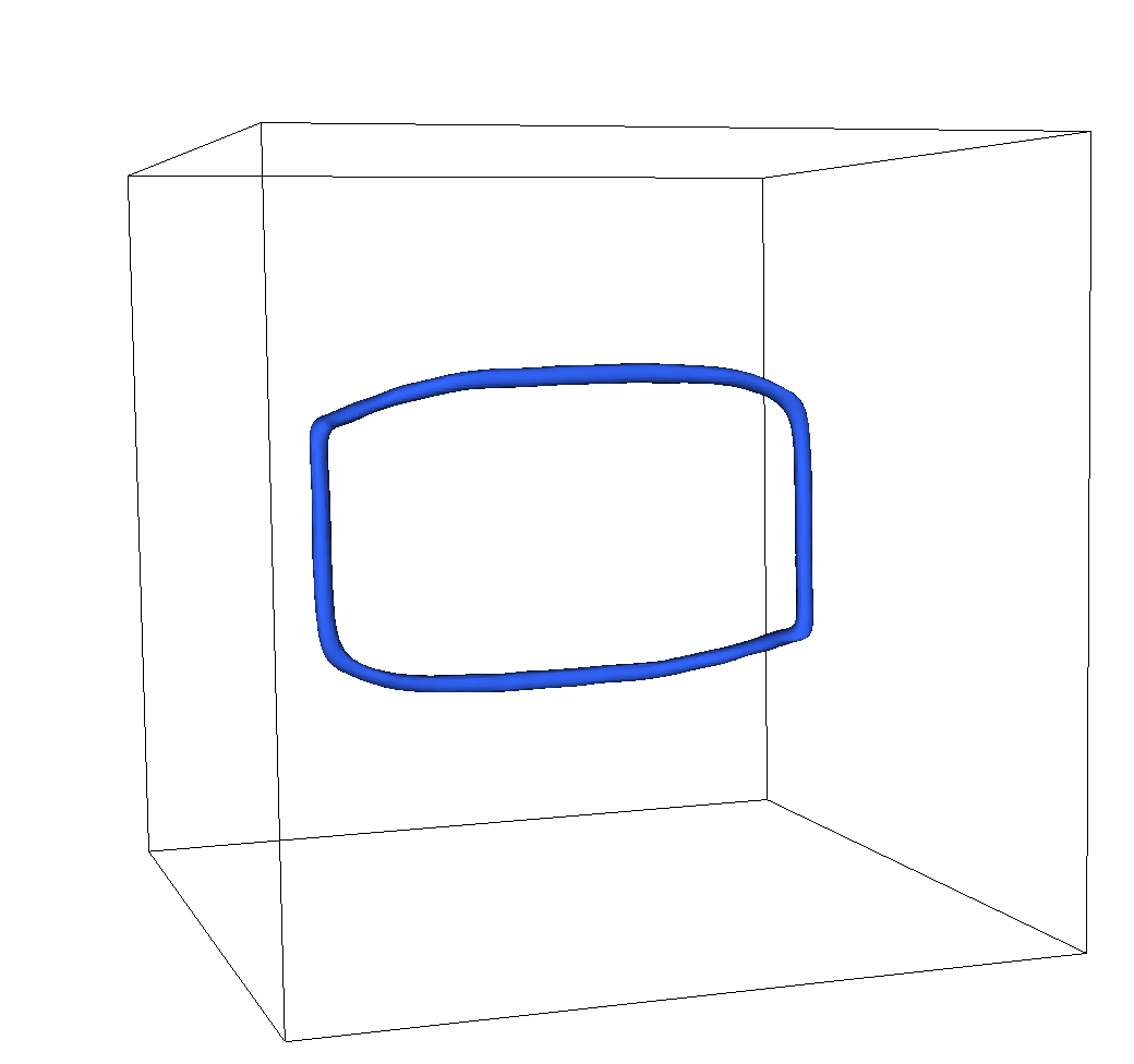
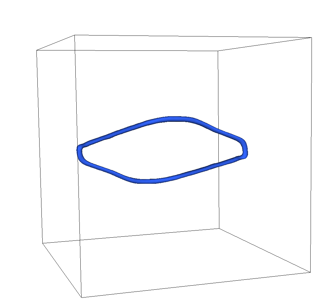
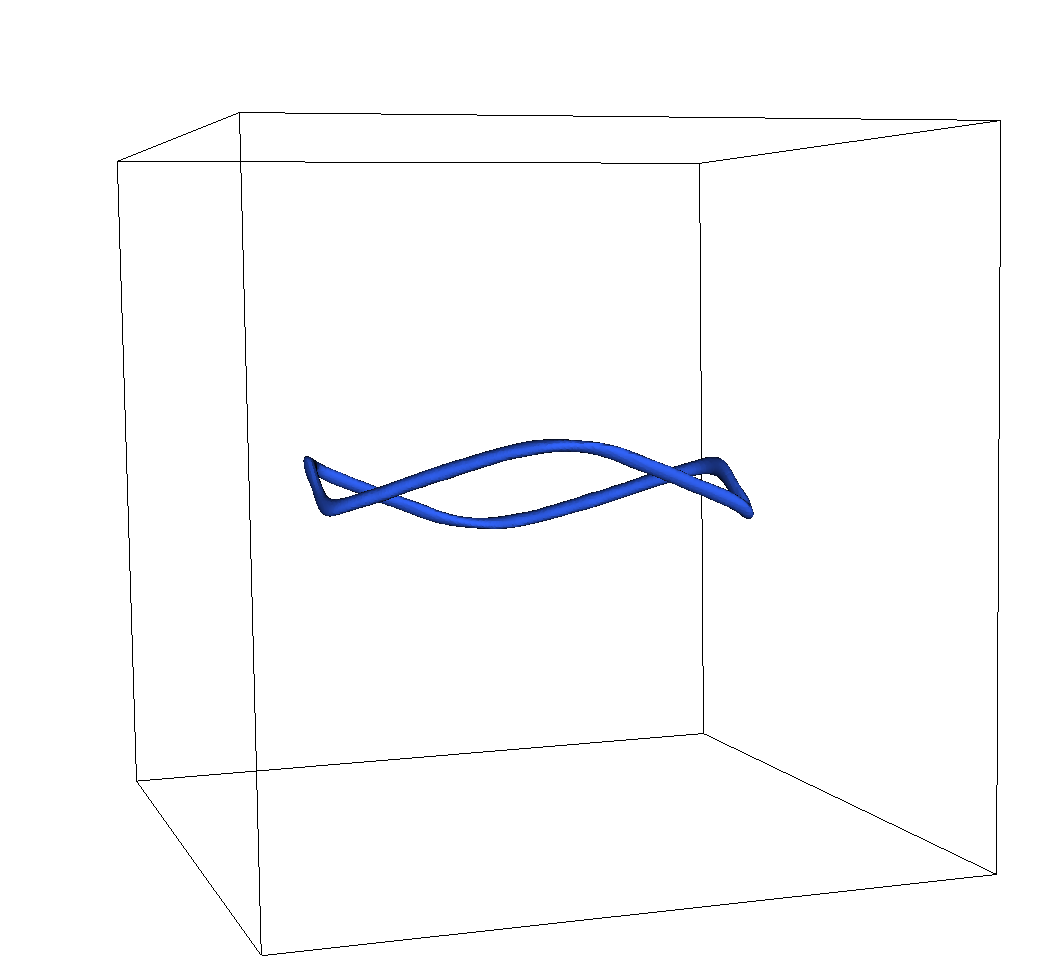
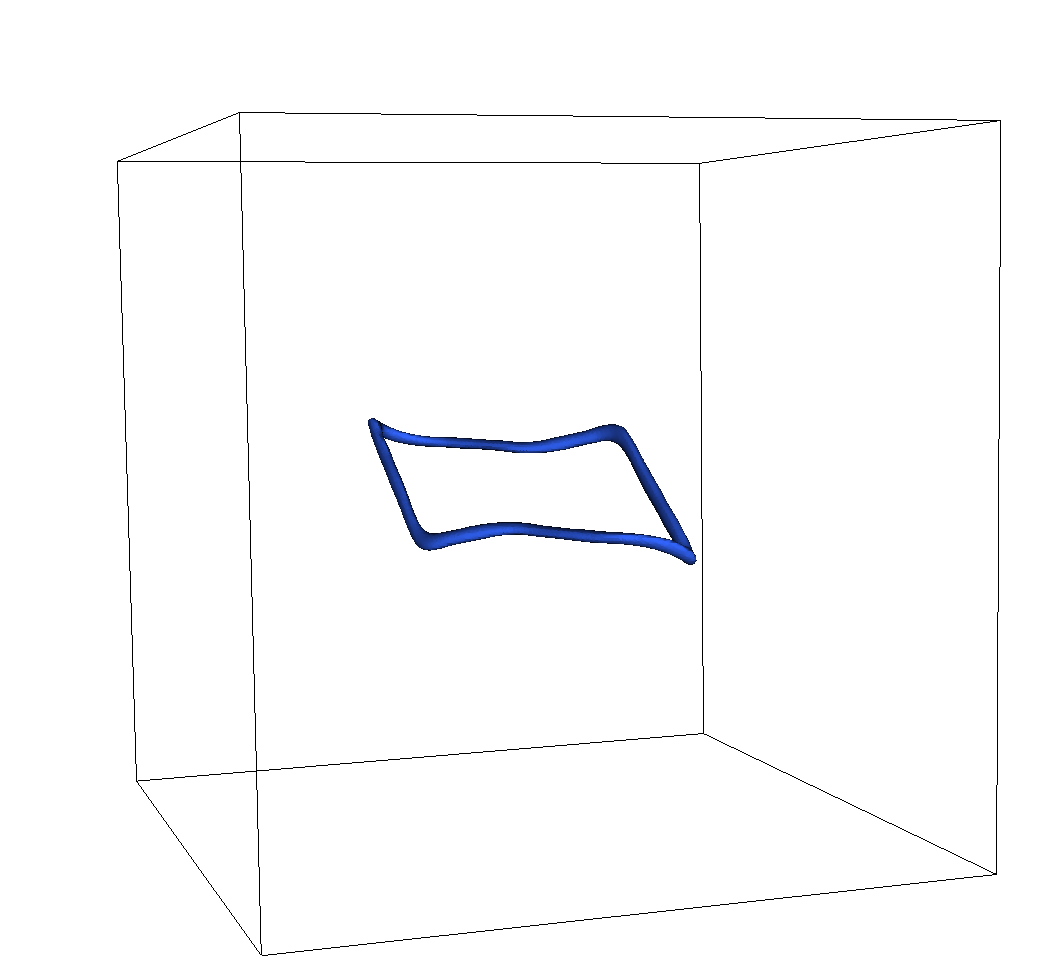
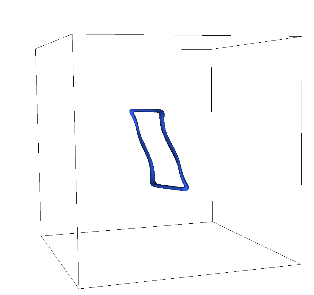
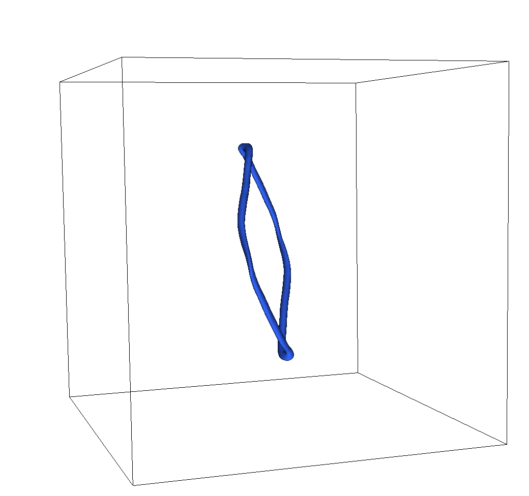
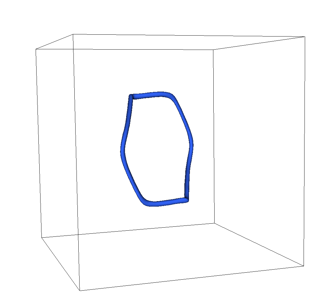
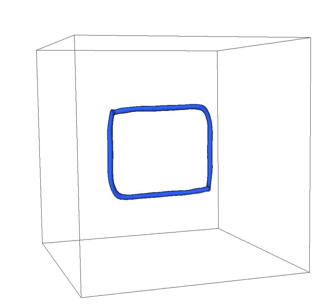
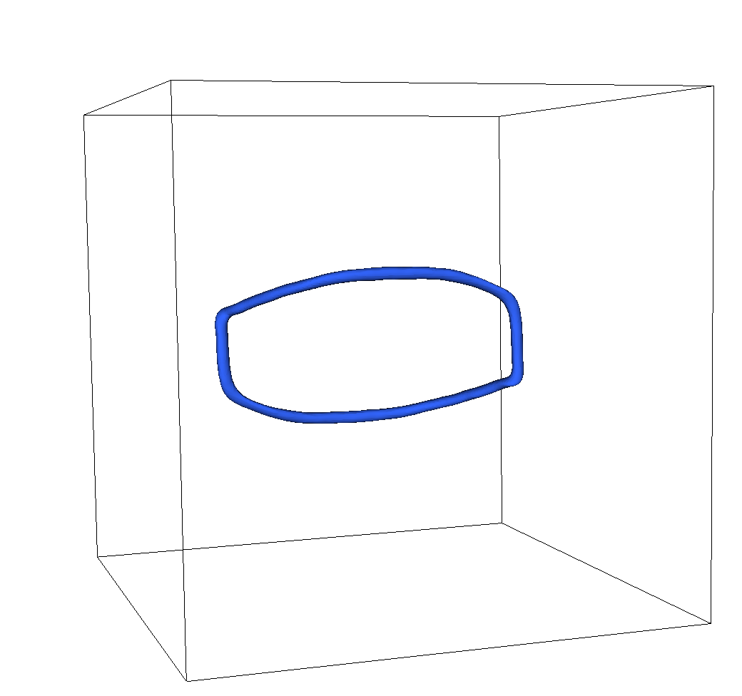
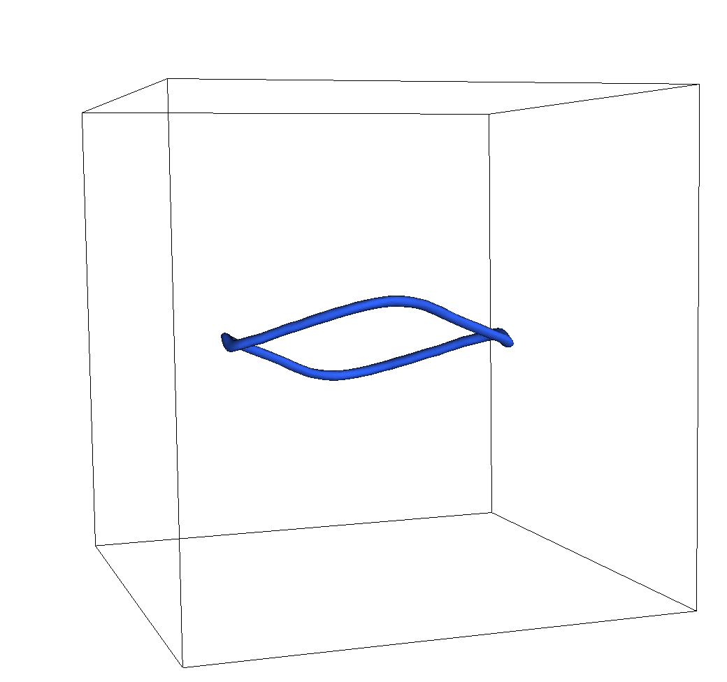
Figure S2: Three-dimensional snapshots of $|\varphi|^{2}=0.2v^{2}$ surfaces of an oscillating artificial loop of type I, simulated with $N=256$, $\delta\tilde{x}=0.25$, $v_{1}=v_{2}=0.25$ and $\sin\alpha=0.4$. Time goes from left to right and from top to bottom, with snapshots separated by $\Delta t=10/\sqrt{\lambda}v$ units of program time. The field has been periodically shifted by $L_{\rm B}/2$ in the $x$ and $z$ directions for clarity in the representation.

Generation of artificial loops of type II. Artificial loops of type II are generated following the procedure introduced in [10, 11]. This is based on initializing static strings of arbitrary shape by setting some magnetic flux on the plaquettes pierced by the initial strings. We note that this techniques relies on the use the hybrid [79, 10] or the compact [33] formulation of the gauge theory on the lattice, in which the field-strength tensor is discretized in terms of the link variables. For our study, we use the hybrid formulation.

Given some shape of the desired one-dimensional strings, one can determine a set of plaquettes pierced by the string. The idea is to set the magnetic flux through these plaquettes to $\pm 2\pi$, depending on the direction from which the plaquette is pierced by the string. This is achieved by setting the gauge variables on the links to

$$A_{\mu}(\bm{n})=\pm\frac{\pi}{2e\delta x}\,,$$ (S14)

where the sign depends on the orientation of link. The complex scalar field is set to be equal to the vacuum expectation value, $\varphi=v$, everywhere. The initial configuration is then diffused for five units of program time, using eq. S2, which leads to the formation of strings with the expected radius, $r_{\text{c}}\sim m_{\text{s}}^{-1}$.

For our study, we use an initial configuration composed by four non-straight static strings, following [11], which intersect soon after the start of the simulation forming two loops. We consider two strings at fixed $y=L_{\rm B}/10$ and $y=9L_{\rm B}/10$ with sinusoidal form. The coordinates of the string core are given by

$$x=\pm A\cos(2\pi z/L_{\rm B})\,,$$ (S15)

with each sign corresponding to a different value of $y$. Also, we set $A=0.075L_{\rm B}$. The other two strings have fixed $z$ with a sawtooth form,

$$x=\left\{\begin{array}[]{ll}\displaystyle\pm C\left[\frac{y}{L_{\rm B}/4}-1\right]\,,&0\leq y\leq L_{\rm B}/2\,,\\[10.0pt] \displaystyle\mp C\left[\frac{y}{L_{\rm B}/4}-3\right]\,,&L_{\rm B}/2<y<L_{\rm B}\,,\end{array}\right.$$ (S16)

with $z=L_{\rm B}/10$ and $z=9L_{\rm B}/10$, for each string, and $C=L_{\rm B}/2$. The signs, again, corresponds to each possible value of $z$. A representation of the resulting configuration at the end the diffusion period, is shown in the left and central panels of fig. S3, from two different perspectives.

aa

Figure S3: Three-dimensional snapshots of $|\varphi|^{2}=0.2v^{2}$ surfaces of the simulation of an artificial loop of type II, corresponding to the end of diffusion (left and center) and the moment in which a single loop is left (right).

After the diffusive phase, the strings are let to evolve in Minkoski spacetime, using a discretization of the equations of motion consistent with the hybrid formulation. The four infinite strings start to move as a result of their non-straight form, and they eventually intersect, forming two loops. Due to the initial position of the infinite strings, the outer one is smaller than the inner one. We wait until the outer loop disappears and study the inner one afterwards. An example of the resulting isolated loop is shown in the right panel of fig. S3.

A drawback of this initialization method is that there remains a magnetic flux frozen on the initialized plaquettes. When measuring the winding number on these plaquettes one finds a non-zero results, which can be associated to a Dirac string [10]. This is an unphysical consequence of this particular initialization procedure, since these Dirac strings do not contain energy, and have not been observed to affect the dynamics of the physical strings. When measuring the length of artificial strings of type II from the number of pierced plaquettes, we subtract the number of initialized plaquettes to the count. For our loops, the number of plaquettes belonging simultaneously to both the real and the ghost string is negligible compared to the total number of plaquettes, and so this does not affect our ability to measure the length of the loops.

Overall, artificial loops of type II are found to behave very similarly to loops of type I. However, loops of type II are typically much smaller than those of type I generated in lattices of the same size. Thus, we consider type II loops to study the power emission of particles, but restrict our investigation on GW emission to type I loops, for simplicity.

Simulation parameters and results. This section summarizes the simulation parameters and the results for the initial length, energy and decay time of different loops considered in this study. Table S1 refers to artificial loops, while table S2 focuses on network loops.

Type I
$v_{1}$	$v_{2}$	$\tilde{L}_{\rm B}$	N	$\delta\tilde{x}$	$\tilde{L}_{\text{av,0}}$	$\tilde{E}_{\text{av,0}}$	$\Delta\tau_{\text{dec}}$
0.6	0.6	126	672	0.1875	272.8	620.4	1902.4
0.6	0.6	147	784	0.1875	319.9	723.0	2594.2
0.6	0.6	168	896	0.1875	361.3	819.9	3322.4
0.6	0.6	189	1008	0.1875	405.9	921.7	4181.5
0.6	0.6	210	1120	0.1875	451.9	1029.3	5180.4
0.6	0.6	98	784	0.125	181.9	408.4	794.0
0.6	0.6	98	784	0.125	239.0	540.6	1429.9
0.6	0.6	98	784	0.125	296.6	678.3	2214.0
0.3	0.6	126	672	0.1875	213.8	480.7	1088.4
0.3	0.6	147	784	0.1875	250.9	562.1	1603.9
0.3	0.6	168	896	0.1875	286.1	643.9	2066.4
0.3	0.6	189	1008	0.1875	322.6	724.2	2721.3
0.3	0.6	210	1120	0.1875	354.0	801.1	3243.2
0.3	0.6	252	1344	0.1875	408.5	936.3	4382.9

Type II
$\tilde{L}_{\rm B}$	N	$\delta\tilde{x}$	$\tilde{L}_{\text{av,0}}$	$\tilde{E}_{\text{av,0}}$	$\Delta\tau_{\text{dec}}$
126	672	0.1875	213.8	480.7	1088.4
147	784	0.1875	250.9	562.1	1603.9
168	896	0.1875	286.1	643.9	2066.4
189	1008	0.1875	322.6	724.2	2721.3
210	1120	0.1875	354.0	801.1	3243.2
252	1344	0.1875	408.5	936.3	4382.9

Table S1: Summary of the simulation parameters (in program units) used to simulate artificial loops of type I (left) and type II (right), together with the results for the oscillation-averaged initial length and energy, and the decay time of the isolated loop obtained after removing the effect from dLC. Type I loops are generated using $\sin\alpha=0.4$.

$\tilde{L}_{\rm B}$	N	$\delta\tilde{x}$	$\tilde{\ell}_{\text{str}}$	$\tilde{L}_{0}$	$\tilde{E}_{\text{str,0}}$	$\Delta\tau_{\text{dec}}$
256	1024	0.25	15	2441.0	4511.4	474
240	960	0.25	15	2306.0	4482.2	421
288	1152	0.25	20	2165.0	3991.9	454
256	1024	0.25	15	2140.0	4238.0	414
256	1024	0.25	15	1774.0	3526.3	311
384	1536	0.25	40	1763.0	3463.9	430
256	1024	0.25	10	1741.0	3335.8	449
240	960	0.25	20	1738.0	3476.7	321
240	960	0.25	20	1727.0	3289.9	380
384	1536	0.25	40	1677.7	3145.2	373
224	896	0.25	12	1646.0	3012.6	352
256	1024	0.25	15	1624.0	3055.4	385
224	896	0.25	12	1476.0	2914.1	332
256	1024	0.25	10	1436.3	2788.8	343
256	1024	0.25	15	1346.7	2588.0	440
256	1024	0.25	15	1297.3	2458.9	252
256	1024	0.25	15	1289.0	2282.3	304
256	1024	0.25	15	1224.0	2299.2	330
256	1024	0.25	15	1183.0	2222.1	337
256	1024	0.25	10	1181.3	2327.6	359
256	1024	0.25	10	1181.0	2289.3	358
256	1024	0.25	10	1117.7	2226.1	362
256	1024	0.25	15	1054.7	2068.8	262
224	896	0.25	12	1053.0	2075.0	217

$\tilde{L}_{\rm B}$	N	$\delta\tilde{x}$	$\tilde{\ell}_{\text{str}}$	$\tilde{L}_{0}$	$\tilde{E}_{\text{str,0}}$	$\Delta\tau_{\text{dec}}$
256	1024	0.25	15	1020.7	2027.1	277
128	512	0.25	8	1019.0	2032.9	213
256	1024	0.25	15	1007.0	1993.2	369
224	896	0.25	12	992.0	1929.4	278
256	1024	0.25	15	979.3	2130.6	266
256	1024	0.25	15	922.0	1779.3	273
224	896	0.25	12	920.0	1582.0	252
128	512	0.25	10	848.3	1622.7	209
256	1024	0.25	15	817.3	1655.0	217
256	1024	0.25	15	793.0	1554.3	273
256	1024	0.25	10	776.0	1573.9	205
240	960	0.25	20	759.0	1748.0	196
128	512	0.25	12	704.7	1424.6	175
256	1024	0.25	15	689.0	1340.3	200
128	512	0.25	15	684.7	1280.5	164
128	512	0.25	10	633.7	1305.9	139
128	512	0.25	15	614.7	1163.0	147
128	512	0.25	12	612.0	1213.8	146
160	1280	0.125	20	607.8	1244.7	181
128	512	0.25	12	551.7	1118.3	142
384	1536	0.25	40	455.7	986.8	134
128	512	0.25	15	432.3	843.6	127
128	512	0.25	8	226.3	508.7	60
128	512	0.25	12	201.3	452.3	40

Table S2: Summary of the simulation parameters (in program units) used to study the decay of network loops, together with the initial length, energy and decay time of the isolated loop.