RECE: Reduced Cross-Entropy Loss for Large-Catalogue Sequential Recommenders

Abstract.

Scalability is a major challenge in modern recommender systems. In sequential recommendations, full Cross-Entropy (CE) loss achieves state-of-the-art recommendation quality but consumes excessive GPU memory with large item catalogs, limiting its practicality.

Using a GPU-efficient locality-sensitive hashing-like algorithm for approximating large tensor of logits, this paper introduces a novel RECE (REduced Cross-Entropy) loss. RECE significantly reduces memory consumption while allowing one to enjoy the state-of-the-art performance of full CE loss. Experimental results on various datasets show that RECE cuts training peak memory usage by up to $12$ times compared to existing methods while retaining or exceeding performance metrics of CE loss. The approach also opens up new possibilities for large-scale applications in other domains.

Figure 1. Simplified example illustrating the bucketing, sorting, chunking, and scalar product calculation steps of the proposed RECE approach. Different colors correspond to belonging to different buckets.

1. Introduction

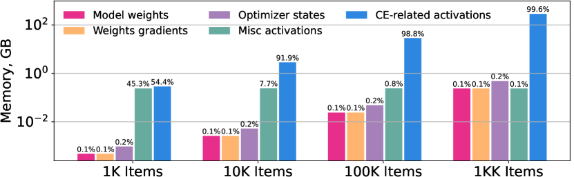
Figure 2. Impact of different components on peak GPU memory usage during SASRec training with Cross-Entropy loss. Measurements were conducted using PyTorch profiling tools.

[]

In collaborative filtering, recent state-of-the-art models increasingly adopt sequential approaches to predict the next item a user might choose based on past activity. By considering the sequence of interactions, such systems make timely and relevant recommendations, like suggesting phone accessories following a phone purchase.

Transformer architectures (Vaswani et al., 2017), originally from natural language processing (NLP), have been successfully adapted for next item prediction task in recommender systems. Notable models include SASRec (Kang and McAuley, 2018) and BERT4Rec (Sun et al., 2019), inspired by GPT (Radford et al., 2018) and BERT (Devlin et al., 2018) architectures. Initially, SASRec employed Binary Cross-Entropy (BCE) loss for training, but subsequent research showed that full Cross-Entropy (CE) loss (3) enables SOTA performance (Klenitskiy and Vasilev, 2023; Petrov and Macdonald, 2023), highlighting CE effectiveness. CE loss, however, is memory-intensive due to the need to compute and store a large tensor of logits, making CE less scalable for larger item catalogs (Fig. 2). The challenge is to develop a reduced replacement for CE loss that maintains accuracy while operating within memory constraints similar to those of BCE.

We propose a novel RECE (REduced Cross-Entropy) loss, which uses a selective computation strategy to prioritize the most informative elements from input sequences and item catalog - those most likely to cause misclassifications. By approximating the softmax distribution over these elements, pre-identified using a GPU-friendly approximate search for maximum inner products, RECE eliminates the need to compute and store the full logit tensor while mitigating inefficiencies of less selective negative sampling. We evaluate RECE integrated into SASRec on four datasets. This approach can also benefit other domains like NLP and search systems.

To summarize, the main contributions of this paper are:

1. We propose RECE – a memory-efficient approximation of CE loss, potentially applicable beyond sequential recommenders;

2. We use RECE to train SASRec, conduct an extensive evaluation, and show that RECE significantly reduces the peak training memory without compromising the model performance.

2. Related Work

Since the introduction of the Transformer architecture (Vaswani et al., 2017), Transformer -based models have outperformed other approaches in sequential recommendations (Sun et al., 2019; Xie et al., 2022; Du et al., 2022). SASRec (Kang and McAuley, 2018) shows state-of-the-art performance with CE loss (Klenitskiy and Vasilev, 2023). However, large item catalogs in real-world applications require negative sampling methods or CE approximations to train such models.

Uniform random sampling of negatives is a straightforward method (Tang and Wang, 2018; Kang and McAuley, 2018). It can be improved by increasing the number of negative samples, modifying BCE (1) or CE (2) (Klenitskiy and Vasilev, 2023) loss functions:

(1) $$\mathcal{L}_{BCE^{+}}=-\log(\sigma(logit_{i,+}))-\sum_{j\in I_{n}^{-}}\log(1-\sigma(logit_{i,j})),$$

(2) $$\mathcal{L}_{CE^{-}}=-\log\frac{\exp(logit_{i,+})}{\exp(logit_{i,+})+\sum_{j\in I_{n}^{-}}\exp(logit_{i,j})},$$

where $I_{n}^{-}$ is a set of $n$ sampled negatives.

However, this method often lacks hard negatives (negatives that the model misclassifies as positives), leading to overconfidence (Petrov and Macdonald, 2023). Calibrating predicted scores can mitigate this (Petrov and Macdonald, 2023), resulting in SOTA performance, but leaves samples uninformative, suggesting possible improvement. Popularity-based sampling (Lian et al., 2020; Chen et al., 2022) is another approach, often better than uniform sampling but still outperformed by methods targeting hard negatives directly (Chen et al., 2022; Rendle and Freudenthaler, 2014). In-batch negative sampling (Hidasi et al., 2015; Hidasi and Karatzoglou, 2018) uses true class labels from other items in the batch, leveraging item popularity. More informative sampling methods approximate softmax distributions using matrix factorizations (Rendle and Freudenthaler, 2014), adaptive n-grams (Bengio and Senécal, 2008), and kernel methods (Blanc and Rendle, 2018; Rawat et al., 2019). Two-step procedures select items with larger logits for loss computation (Bai et al., 2017; Chen et al., 2022; Wilm et al., 2023). Methods targeting hard negatives include accumulating hard negatives for each user (Wang et al., 2021; Ding et al., 2020), but this introduces memory overhead. Instead, hard negatives can be selected at each step using (approximate) maximum inner product search (MIPS) or nearest neighbor search (NNS) (Vijayanarasimhan et al., 2014; Spring and Shrivastava, 2017; Guo et al., 2016; Yen et al., 2018; Lian et al., 2020). However, the implementations of these methods are not designed for GPU usage and are not easily adaptable due to their reliance on GPU-inefficient operations (like maintaining a hash table).

In summary, existing methods fail to target hard negatives effectively or are inefficient for GPU computations, resulting in suboptimal model performance. Our approach addresses this by ensuring an efficient search for hard negatives and batch processing compatibility, which improves GPU utilization.

3. Reduced Cross-Entropy

In this section, we propose a novel scalable approach for CE loss approximation that reduces memory requirements while maintaining performance, and discuss its wide applicability across domains.

Inspired by the studies (Kitaev et al., 2020) for efficient attention approximation, our method utilizes locality-sensitive hashing for angular distance (Andoni et al., 2015) for the calculation of CE loss over the part of catalog that most affects gradient updates, finding this part in a GPU-friendly manner.

If we are predicting the next item $z_{i+1}$ (catalog index) for item $z_{i}$, with $x_{i}$ as the transformer’s output for $z_{i}$, $y_{j}$ as the embedding of item $j$ (both of dimension $d$) and the model output score $logit_{i,j}=x_{i}^{T}y_{j}$, then for catalog size $C$, the CE loss for item $z_{i}$:

(3) $$\mathcal{L}_{CE}=-\log(\text{softmax}(logit_{i})_{z_{i+1}})\ =-\log\frac{\exp(logit_{i,z_{i+1}})}{\sum_{c=1}^{C}\exp(logit_{i,c})}$$

(4) $$\frac{\partial\mathcal{L}_{CE}}{\partial logit_{i,k}}=\text{softmax}(logit_{i})_{k}-\mathds{1}[k=z_{i+1}]\in\left(-1,1\right)$$

The gradient of the CE loss with respect to logits ranges from $-1$ to $1$ (Eq. 4). It is close to $1$ for high predicted probabilities of incorrect classes and close to $-1$ for low predicted probabilities of correct classes. We aim to compute only logits with the largest absolute gradient values to preserve the most information, identifying these cases in advance. While the correct class logit is known, finding large logits for negative classes is a harder task. We simplify this by searching for all large logits, essentially solving a MIPS problem.

To address this task, we propose the RECE approach, presented in Algorithm 1 with Lines 3-12 depicted in Fig. 1. It starts by generating a set $B$ of $n_{b}$ random vectors (Line 2), then indexing of the transformer outputs $X$ (dimensions for batch size $s$ and sequence length $l$ are collapsed) and catalog item embeddings $Y$ with the index of the nearest vector from $B$ (Lines 3-4). We want to divide items from $X$ and $Y$ into groups based on these indices and to calculate logits only within groups. The idea is that two vectors sharing the nearest vector (in terms of dot product) are likely close to each other. The sizes of these groups could be different, and to perform later computations efficiently, we sort elements based on new indices and divide them into $n_{c}$ equal-sized chunks (Lines 5-11). The number of chunks $n_{c}$ can be selected larger than $n_{b}$ so that relevant items fall into the same chunk with a higher probability. For the same reason, for logit calculation, we also select items from the neighboring chunks (Line 12). Finally, we calculate logits for negative classes within chunks, compute positive logits ($\hat{Z}$ – correct predictions matrix), determine the value of the loss function for each chunk, and average these values across chunks (Lines 12-16). For better performance, the described procedure (Lines 2-12) can be repeated in parallel over several rounds $r$. In this case, the value of loss function is calculated over an enriched set of negative examples. Duplicate item pairs are accounted for by subtracting from the calculated logit value the natural logarithm of the number of times the logit between these items was calculated over all rounds. For the experiments, we chose the optimal, in terms of peak memory, number of random vectors ($n_{b}^{*}=\sqrt{4\alpha_{bc}(1+2n_{ec})\cdot\min(C,s\cdot l)}$, where $\alpha_{bc}=n_{b}/n_{c}$, $n_{ec}$ is the number of neighboring chunks we look into). The memory complexity of our algorithm is then $2r\sqrt{\alpha_{bc}(1+2n_{ec})\cdot\min(C,s\cdot l)}\cdot\max(C,s\cdot l)$. This is $\sqrt{\min(C,s\cdot l)}/(2r\sqrt{\alpha_{bc}(1+2n_{ec})})$ times smaller than the memory size required for the full Cross-Entropy loss. The extended derivation is available in our GitHub repository2.

Algorithm 1 Reduced Cross-Entropy Loss

1:Input: $\hat{Z}\in\mathbb{N}^{s\cdot l}$, $X\in\mathbb{R}^{s\cdot l\times d}$, $Y\in\mathbb{R}^{C\times d}$, $n_{b}$, $n_{c}$

2:$B=\text{randn}_{\scriptstyle{\mathcal{N}(0,1)}}(n_{b},d)=\{b_{k}\}_{k=1}^{n_{b}}$

3:$I=\text{argmax}_{b}\text{ }BX^{\top}$ $\triangleright$ index of nearest $b_{k}$

4:$J=\text{argmax}_{b}\text{ }BY^{\top}$

5:$X=X[\text{argsort }I]$ $\triangleright$ sorting based on new index

6:$Y=Y[\text{argsort }J]$

7:for $c$ in range($n_{c}$): $\triangleright$ divide into $n_{c}$ chunks

8:      $I_{c}=\{i:c|X|/n_{c}\leq i<(c+1)|X|/n_{c}\}$

9:      $J_{c}=\{j:c|Y|/n_{c}\leq j<(c+1)|Y|/n_{c}\}$

10:      $X_{c}=X[I_{c}]$

11:      $Y_{c*}=Y[J_{c-1}\cup J_{c}\cup J_{c+1}]$ $\triangleright$ current and adjacent chunks

12:      $logits^{-}_{c}=X_{c}{Y^{\top}}_{c*}\in\mathbb{R}^{|X|/n_{c}\times 3|Y|/n_{c}}$ $\triangleright$ logits for wrong classes

13:      for $i$ in range($|X|/n_{c}$):

14:           $logit^{+}_{c,i}=\sum_{k=1}^{d}X[I_{c,i}]_{k}\cdot Y[\hat{Z}[I_{c,i}]]_{k}$ $\triangleright$ logit for correct class

15:           $loss_{c,i}=-\log\frac{\exp(logit^{+}_{c,i})}{\exp(logit^{+}_{c,i})+\sum_{j=1}^{3|Y|/n_{c}}\exp(logits^{-}_{c,i,j})}$

16:$\mathcal{L}_{\text{RECE}}=\frac{1}{|X|}\sum_{c,i}loss_{c,i}$ $\triangleright$ accumulation of loss values

In this work, we utilize SASRec (Kang and McAuley, 2018) as our base model due to its widespread use in the literature (Tian et al., 2022; Petrov and Macdonald, 2023) and its state-of-the-art performance in sequential recommendations with full Cross-Entropy loss (Klenitskiy and Vasilev, 2023). Although our primary focus on the RECE method is on recommender systems, where managing large catalogs is a common challenge, the applicability of this approach extends to various domains such as NLP, search systems, computer vision tasks, bioinformatics, and other areas, where tasks with extensive vocabularies or large number of classes are a common bottleneck.

4. Experimental Settings

Datasets

We conduct our main experiments on four diverse real-world datasets: BeerAdvocate (McAuley et al., 2012), Behance (He et al., 2016), Amazon Kindle Store (Ni et al., 2019), and Gowalla (Cho et al., 2011). In line with previous research (Tang and Wang, 2018; Kang and McAuley, 2018; Sun et al., 2019), we interpret the presence of a review or rating as implicit feedback. Additionally, following common practice (Kang and McAuley, 2018; Rendle et al., 2010; Zhang et al., 2019) and to ensure the number of items in datasets allows for computing full Cross-Entropy loss within GPU memory constraints, we exclude unpopular items with fewer than $5$ interactions and remove users who have fewer than $20$ interactions. The final dataset statistics are summarized in Table 1. The number of items ranges from $22,307$ in BeerAdvocate to $173,511$ in Gowalla, allowing us to evaluate methods under various memory consumption conditions.

Table 1. Statistics of the datasets after preprocessing.

Dataset	Domain	Users	Items	Interactions	Density
BeerAdvocate (McAuley et al., 2012)	Food	7,606	22,307	1,409,494	0.83%
Behance (He et al., 2016)	Art	8,097	32,434	546,284	0.21%
Kindle Store (Ni et al., 2019)	E-com	23,684	96,830	1,256,065	0.05%
Gowalla (Cho et al., 2011)	Soc. Net.	27,516	173,511	2,627,663	0.06%

Evaluation

In offline testing, data splitting using the leave-one-out approach, often by selecting each user’s last interaction, is common in previous studies (Petrov and Macdonald, 2023; Klenitskiy and Vasilev, 2023). However, this method can lead to data leakage affecting evaluation accuracy (Ji et al., 2023; Meng et al., 2020). To mitigate this, we set a global timestamp at the $0.95$ quantile of all interactions (Frolov and Oseledets, 2022). Interactions before this timestamp are used for training, while interactions after – for testing, keeping test users separate from the training data (Fig. 3). For test users, we use their last interaction to evaluate model performance. This temporal split prevents ”recommendations from future” bias (Meng et al., 2020), ensuring the model remains unaware of future interactions. In addition, we use the second-to-last interaction of each test user for validation to tune the model and to control its convergence via early stopping.

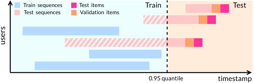
Figure 3. Temporal data splitting strategy.

[]

Following best practices (Dallmann et al., 2021; Cañamares and Castells, 2020), we use unsampled top-K ranking metrics: Normalized Discounted Cumulative Gain (NDCG@K) and Hit Rate (HR@K), with K $=1,5,10$. Our goal is to balance time consumption, memory efficiency, and ranking performance, so we also measure training time and peak GPU memory during training.

Model and Baselines

In our experiments, we use SASRec as the base model and enhance it with the proposed RECE loss. We focus on comparing SASRec-RECE with the model incorporating Binary Cross-Entropy loss with multiple negative samples (SASRec-BCE⁺), detailed in Eq. (1), and with SASRec employing full Cross-Entropy loss (SASRec-CE). Furthermore, we explore recent SOTA sampling-based variations of the loss function for SASRec proposed by Klenitskiy et al. (Klenitskiy and Vasilev, 2023) and Petrov et al. (Petrov and Macdonald, 2023), denoted SASRec-CE^- and gSASRec (gBCE loss) respectively. All models are based on the adapted PyTorch implementation of the original SASRec architecture, and augmented with loss functions and sampling strategies from the respective papers. All code is available in our repository.

5. Results

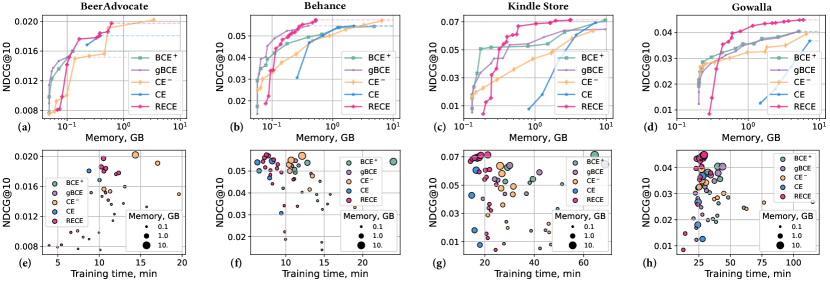
Figure 4. (a)-(d) Pareto front curves illustrating NDCG@10 for different memory budgets. (e)-(h) Same points plotted on NDCG@10 vs. Training time axes, with point sizes representing memory values from corresponding (a)-(d) plots.

Our experiments indicate that when $n_{c}$ is equal to $n_{b}$ ($\alpha_{bc}=1$), optimal performance is achieved for a given memory limit, provided that $n_{ec}$ is sufficiently large. The number of extra neighboring chunks $n_{ec}$ and the number of rounds $r$ should be increased for larger batch sizes. To demonstrate the effectiveness of our approach, we conducted a series of experiments in the quality-memory trade-off paradigm on a set of datasets (Section 4), comparing the SASRec-RECE model with baselines described in Section 4. In order to obtain quality metrics (NDCG@10) for different memory values, we evaluated these models for different values of hyperparameters affecting peak memory: batch size, number of negative samples for BCE⁺, gBCE, and CE^-, $n_{ec}$ and $r$ for RECE. The grids for all parameters are available in our GitHub2. Figure 4 shows optimal points for given memory budgets, dashed line means there was no configuration that showed higher quality at increased budget.

On BeerAdvocate, the dataset with a small catalog, SASRec-RECE achieves performance close to the best competitors (Fig. 4a), both in terms of quality and peak memory. However, our method is more effective on datasets with larger catalogs, where the memory consumption problem becomes more pronounced. On Behance and Kindle Store datasets (Fig. 4b-c), RECE provides nearly the same quality with 12 (0.526GB vs. 6.48GB) and 3 (3.15GB vs. 9.73GB) times less memory consumed, respectively, while on the Gowalla (dataset with the largest catalog) (Fig. 4d), RECE can either outperform the second best method by 8.19% (0.0449 vs. 0.0415 NDCG@10) or yield almost the same quality with 6.6 times less memory (0.78GB vs. 5.13GB). We can also see that SASRec-RECE does not produce any significant computational overhead, and its training time is at the lower end of the spectrum within the competitors (Fig. 4e-h). Table 2 shows the extended set of metrics for the largest datasets.

Table 2. Performance under memory constraints. Bold indicates the best performance, and underlined is the second-best. NDCG@1 and HR@1 are equivalent by definition.

Dataset	Model	NDCG@1	NDCG@5	NDCG@10	HR@5	HR@10
Kindle Store	BCE+	0.0473	0.0674	0.0725	0.0856	0.1010
	gBCE	0.0473	0.0626	0.0681	0.0766	0.0933
	CE-	0.0397	0.0582	0.0644	0.0744	0.0938
	CE	0.0467	0.0658	0.0711	0.0822	0.0972
	RECE	0.0486	0.0665	0.0714	0.0822	0.0985
Gowalla	BCE+	0.0175	0.0341	0.0415	0.0507	0.0739
	gBCE	0.0165	0.0337	0.0410	0.0506	0.0733
	CE-	0.0162	0.0321	0.0402	0.0475	0.0729
	CE	0.0164	0.0324	0.0388	0.0471	0.0674
	RECE	0.0192	0.0372	0.0449	0.0546	0.0787

Finally, following (Petrov and Macdonald, 2023), we evaluate SASRec-RECE on the Amazon Beauty dataset (McAuley et al., 2015) against recent models, which report best results, including CBiT (Du et al., 2022), DuoRec (Qiu et al., 2022), CL4SRec (Xie et al., 2022), and FEARec (Du et al., 2023). To comply with the evaluation protocols of these works, we replace the temporal data splitting strategy, described in Section 4, with the leave-one-out evaluation approach and the corresponding data preprocessing. Table 3 shows that SASRec-RECE achieves performance comparable to the recently proposed models.

Table 3. Comparison of SASRec-RECE with recent results on Beauty using leave-one-out splitting strategy. Setup follows (Petrov and Macdonald, 2023). Best values are in bold, second best are underlined.

Metric	FEARec	CBiT	DuoRec	CL4SRec	SASRec-RECE
NDCG@10	0.0459	0.0537	0.0443	0.0299	0.0525
HR@10	0.0884	0.0905	0.0845	0.0681	0.0897

6. Conclusion

In this work, we introduced RECE, a novel loss function that approximates full Cross-Entropy using hard-negative mining with GPU-efficient operations. This allows the benefits of CE loss, known for state-of-the-art performance, to be applied to large catalogs that would otherwise be infeasible due to high memory requirements. We demonstrated that RECE almost matches the performance and memory requirements of recent negative sampling methods on datasets with small catalogs and consumes up to $12$ times less memory on large-catalog datasets. Alternatively, it can improve quality (NDCG@10) by up to $8.19\%$ compared to other approaches if provided with an extended memory budget. The idea behind RECE can potentially be applied not only to other loss functions and models in sequential recommender systems but also to other domains.

- (1)
- Andoni et al. (2015) Alexandr Andoni, Piotr Indyk, Thijs Laarhoven, Ilya Razenshteyn, and Ludwig Schmidt. 2015. Practical and optimal LSH for angular distance. Advances in neural information processing systems 28 (2015).
- Bai et al. (2017) Yu Bai, Sally Goldman, and Li Zhang. 2017. Tapas: Two-pass approximate adaptive sampling for softmax. arXiv preprint arXiv:1707.03073 (2017).
- Bengio and Senécal (2008) Yoshua Bengio and Jean-Sébastien Senécal. 2008. Adaptive importance sampling to accelerate training of a neural probabilistic language model. IEEE Transactions on Neural Networks 19, 4 (2008), 713–722.
- Blanc and Rendle (2018) Guy Blanc and Steffen Rendle. 2018. Adaptive sampled softmax with kernel based sampling. In International conference on machine learning. PMLR, 590–599.
- Cañamares and Castells (2020) Rocío Cañamares and Pablo Castells. 2020. On Target Item Sampling in Offline Recommender System Evaluation. 259–268. https://doi.org/10.1145/3383313.3412259
- Chen et al. (2022) Yongjun Chen, Jia Li, Zhiwei Liu, Nitish Shirish Keskar, Huan Wang, Julian McAuley, and Caiming Xiong. 2022. Generating Negative Samples for Sequential Recommendation. arXiv preprint arXiv:2208.03645 (2022).
- Cho et al. (2011) Eunjoon Cho, Seth A. Myers, and Jure Leskovec. 2011. Friendship and mobility: user movement in location-based social networks. In Knowledge Discovery and Data Mining.
- Dallmann et al. (2021) Alexander Dallmann, Daniel Zoller, and Andreas Hotho. 2021. A Case Study on Sampling Strategies for Evaluating Neural Sequential Item Recommendation Models. In Fifteenth ACM Conference on Recommender Systems (RecSys ’21). ACM. https://doi.org/10.1145/3460231.3475943
- Devlin et al. (2018) Jacob Devlin, Ming-Wei Chang, Kenton Lee, and Kristina Toutanova. 2018. Bert: Pre-training of deep bidirectional transformers for language understanding. arXiv preprint arXiv:1810.04805 (2018).
- Ding et al. (2020) Jingtao Ding, Yuhan Quan, Quanming Yao, Yong Li, and Depeng Jin. 2020. Simplify and robustify negative sampling for implicit collaborative filtering. Advances in Neural Information Processing Systems 33 (2020), 1094–1105.
- Du et al. (2022) Hanwen Du, Hui Shi, Pengpeng Zhao, Deqing Wang, Victor S. Sheng, Yanchi Liu, Guanfeng Liu, and Lei Zhao. 2022. Contrastive Learning with Bidirectional Transformers for Sequential Recommendation. arXiv:2208.03895 [cs.IR]
- Du et al. (2023) Xinyu Du, Huanhuan Yuan, Pengpeng Zhao, Fuzhen Zhuang, Guanfeng Liu, and Yanchi Liu. 2023. Frequency Enhanced Hybrid Attention Network for Sequential Recommendation.
- Frolov and Oseledets (2022) Evgeny Frolov and Ivan Oseledets. 2022. Tensor-based Sequential Learning via Hankel Matrix Representation for Next Item Recommendations. arXiv:2212.05720 [cs.LG]
- Guo et al. (2016) Ruiqi Guo, Sanjiv Kumar, Krzysztof Choromanski, and David Simcha. 2016. Quantization based fast inner product search. In Artificial intelligence and statistics. PMLR, 482–490.
- He et al. (2016) Ruining He, Chen Fang, Zhaowen Wang, and Julian McAuley. 2016. Vista: A Visually, Socially, and Temporally-aware Model for Artistic Recommendation. In Proceedings of the 10th ACM Conference on Recommender Systems (RecSys ’16). ACM. https://doi.org/10.1145/2959100.2959152
- Hidasi and Karatzoglou (2018) Balázs Hidasi and Alexandros Karatzoglou. 2018. Recurrent neural networks with top-k gains for session-based recommendations. In Proceedings of the 27th ACM international conference on information and knowledge management. 843–852.
- Hidasi et al. (2015) Balázs Hidasi, Alexandros Karatzoglou, Linas Baltrunas, and Domonkos Tikk. 2015. Session-based recommendations with recurrent neural networks. arXiv preprint arXiv:1511.06939 (2015).
- Ji et al. (2023) Yitong Ji, Aixin Sun, Jie Zhang, and Chenliang Li. 2023. A Critical Study on Data Leakage in Recommender System Offline Evaluation. ACM Transactions on Information Systems 41, 3 (Feb. 2023), 1–27. https://doi.org/10.1145/3569930
- Kang and McAuley (2018) Wang-Cheng Kang and Julian McAuley. 2018. Self-attentive sequential recommendation. In 2018 IEEE international conference on data mining (ICDM). IEEE, 197–206.
- Kitaev et al. (2020) Nikita Kitaev, Łukasz Kaiser, and Anselm Levskaya. 2020. Reformer: The efficient transformer. arXiv preprint arXiv:2001.04451 (2020).
- Klenitskiy and Vasilev (2023) Anton Klenitskiy and Alexey Vasilev. 2023. Turning Dross Into Gold Loss: is BERT4Rec really better than SASRec?. In Proceedings of the 17th ACM Conference on Recommender Systems (RecSys ’23). ACM. https://doi.org/10.1145/3604915.3610644
- Lian et al. (2020) Defu Lian, Qi Liu, and Enhong Chen. 2020. Personalized ranking with importance sampling. In Proceedings of The Web Conference 2020. 1093–1103.
- McAuley et al. (2012) Julian McAuley, Jure Leskovec, and Dan Jurafsky. 2012. Learning attitudes and attributes from multi-aspect reviews. In 2012 IEEE 12th International Conference on Data Mining. IEEE, 1020–1025.
- McAuley et al. (2015) Julian McAuley, Christopher Targett, Qinfeng Shi, and Anton van den Hengel. 2015. Image-based Recommendations on Styles and Substitutes. arXiv:1506.04757 [cs.CV]
- Meng et al. (2020) Zaiqiao Meng, Richard McCreadie, Craig Macdonald, and Iadh Ounis. 2020. Exploring Data Splitting Strategies for the Evaluation of Recommendation Models. arXiv:2007.13237 [cs.IR]
- Ni et al. (2019) Jianmo Ni, Jiacheng Li, and Julian McAuley. 2019. Justifying Recommendations using Distantly-Labeled Reviews and Fine-Grained Aspects. 188–197. https://doi.org/10.18653/v1/D19-1018
- Petrov and Macdonald (2023) Aleksandr Vladimirovich Petrov and Craig Macdonald. 2023. gSASRec: Reducing Overconfidence in Sequential Recommendation Trained with Negative Sampling. In Proceedings of the 17th ACM Conference on Recommender Systems (RecSys ’23). ACM. https://doi.org/10.1145/3604915.3608783
- Qiu et al. (2022) Ruihong Qiu, Zi Huang, Hongzhi Yin, and Zijian Wang. 2022. Contrastive Learning for Representation Degeneration Problem in Sequential Recommendation. 813–823. https://doi.org/10.1145/3488560.3498433
- Radford et al. (2018) Alec Radford, Karthik Narasimhan, Tim Salimans, Ilya Sutskever, et al. 2018. Improving language understanding by generative pre-training. (2018).
- Rawat et al. (2019) Ankit Singh Rawat, Jiecao Chen, Felix Xinnan X Yu, Ananda Theertha Suresh, and Sanjiv Kumar. 2019. Sampled softmax with random fourier features. Advances in Neural Information Processing Systems 32 (2019).
- Rendle and Freudenthaler (2014) Steffen Rendle and Christoph Freudenthaler. 2014. Improving pairwise learning for item recommendation from implicit feedback. In Proceedings of the 7th ACM international conference on Web search and data mining. 273–282.
- Rendle et al. (2010) Steffen Rendle, Christoph Freudenthaler, and Lars Schmidt-Thieme. 2010. Factorizing personalized markov chains for next-basket recommendation. In Proceedings of the 19th international conference on World wide web. 811–820.
- Spring and Shrivastava (2017) Ryan Spring and Anshumali Shrivastava. 2017. A new unbiased and efficient class of lsh-based samplers and estimators for partition function computation in log-linear models. arXiv preprint arXiv:1703.05160 (2017).
- Sun et al. (2019) Fei Sun, Jun Liu, Jian Wu, Changhua Pei, Xiao Lin, Wenwu Ou, and Peng Jiang. 2019. BERT4Rec: Sequential recommendation with bidirectional encoder representations from transformer. In Proceedings of the 28th ACM international conference on information and knowledge management. 1441–1450.
- Tang and Wang (2018) Jiaxi Tang and Ke Wang. 2018. Personalized top-n sequential recommendation via convolutional sequence embedding. In Proceedings of the eleventh ACM international conference on web search and data mining. 565–573.
- Tian et al. (2022) Changxin Tian, Zihan Lin, Shuqing Bian, Jinpeng Wang, and Wayne Zhao. 2022. Temporal Contrastive Pre-Training for Sequential Recommendation. 1925–1934. https://doi.org/10.1145/3511808.3557468
- Vaswani et al. (2017) Ashish Vaswani, Noam Shazeer, Niki Parmar, Jakob Uszkoreit, Llion Jones, Aidan N Gomez, Łukasz Kaiser, and Illia Polosukhin. 2017. Attention is all you need. Advances in neural information processing systems 30 (2017).
- Vijayanarasimhan et al. (2014) Sudheendra Vijayanarasimhan, Jonathon Shlens, Rajat Monga, and Jay Yagnik. 2014. Deep networks with large output spaces. arXiv preprint arXiv:1412.7479 (2014).
- Wang et al. (2021) Jinpeng Wang, Jieming Zhu, and Xiuqiang He. 2021. Cross-batch negative sampling for training two-tower recommenders. In Proceedings of the 44th international ACM SIGIR conference on research and development in information retrieval. 1632–1636.
- Wilm et al. (2023) Timo Wilm, Philipp Normann, Sophie Baumeister, and Paul-Vincent Kobow. 2023. Scaling Session-Based Transformer Recommendations using Optimized Negative Sampling and Loss Functions. In Proceedings of the 17th ACM Conference on Recommender Systems. 1023–1026.
- Xie et al. (2022) Xu Xie, Fei Sun, Zhaoyang Liu, Shiwen Wu, Jinyang Gao, Jiandong Zhang, Bolin Ding, and Bin Cui. 2022. Contrastive Learning for Sequential Recommendation. 2022 IEEE 38th International Conference on Data Engineering (ICDE) (2022), 1259–1273. https://api.semanticscholar.org/CorpusID:251299631
- Yen et al. (2018) Ian En-Hsu Yen, Satyen Kale, Felix Yu, Daniel Holtmann-Rice, Sanjiv Kumar, and Pradeep Ravikumar. 2018. Loss decomposition for fast learning in large output spaces. In International Conference on Machine Learning. PMLR, 5640–5649.
- Zhang et al. (2019) Tingting Zhang, Pengpeng Zhao, Yanchi Liu, Victor S. Sheng, Jiajie Xu, Deqing Wang, Guanfeng Liu, and Xiaofang Zhou. 2019. Feature-level Deeper Self-Attention Network for Sequential Recommendation. In International Joint Conference on Artificial Intelligence.