Explosive neural networks via higher-order interactions in curved statistical manifolds

Abstract

Higher-order interactions underlie complex phenomena in systems such as biological and artificial neural networks, but their study is challenging due to the lack of tractable standard models. By leveraging the maximum entropy principle in curved statistical manifolds, here we introduce curved neural networks as a class of prototypical models for studying higher-order phenomena. Through exact mean-field descriptions, we show that these curved neural networks implement a self-regulating annealing process that can accelerate memory retrieval, leading to explosive order-disorder phase transitions with multi-stability and hysteresis effects. Moreover, by analytically exploring their memory capacity using the replica trick near ferromagnetic and spin-glass phase boundaries, we demonstrate that these networks enhance memory capacity over the classical associative-memory networks. Overall, the proposed framework provides parsimonious models amenable to analytical study, revealing novel higher-order phenomena in complex network systems.

Complex physical, biological, and social systems often exhibit higher-order interdependencies that cannot be reduced to pairwise interactions between their components [1, 2]. Recent studies suggest that higher-order organisation is not the exception but the norm, providing various mechanisms for its emergence [3, 4, 5, 6]. Modelling studies have revealed that higher-order interactions (HOIs) underlie collective activities such as bistability, hysteresis, and ‘explosive’ phase transitions associated with abrupt discontinuities in order parameters [7, 8, 9, 10, 4, 11].

HOIs are particularly important for the functioning of biological and artificial neural systems. For instance, they shape the collective activity of biological neurons  [12, 13], being directly responsible for their inherent sparsity [14, 13, 15, 5] and possibly underlying critical dynamics [16, 17]. HOIs have also been shown to enhance the computational capacity of artificial recurrent neural networks [18, 19]. More specifically, ‘dense associative memories’ with extended memory capacity [20, 21] are realised by specific non-linear activation functions, which effectively incorporate HOIs. These non-linear functions are related to attention mechanisms of transformer neural networks [22] and the energy landscape of diffusion models [23, 24], leading to conjecture that HOIs underlie the success of these state-of-the-art deep learning models.

Despite their importance, existent studies of HOIs are limited by key computational challenges, as an exhaustive representation of HOIs results in a combinatorial explosion [25]. This issue is pervasive, restricting investigations of high-order interaction models — such as contagion [9], Ising [19] or Kuramoto [26] models — to highly homogeneous scenarios [3, 16] or to models of relatively low-order [27, 9, 11]. In fact, it is currently unclear how to construct tractable models to address the diverse effects of HOIs in a principled manner.

To address this challenge, we use an extension of Shannon’s maximum entropy framework to capture HOIs through the deformation of the space of statistical models. When applied to neural networks, our approach generalises classical neural network models to yield a family of curved neural networks, which effectively incorporate HOIs even if the model’s statistics are restricted to low-order. Our framework establishes rich connections with the literature on the statistical physics of neural networks, enabling explorations of various aspects of HOIs using techniques including mean-field approximations, quenched disorder analyses, and path integrals.

Our results show that relatively simple curved neural networks display hallmarks of higher-order phenomena such as explosive phase transitions — both in simple mean-field models and also in more complex phase transitions to spin-glass states. These phenomena are driven by a self-regulated annealing process, which accelerates memory retrieval through positive feedback between energy and an ‘effective’ temperature. Furthermore, we show — both analytically and experimentally — that this mechanism leads to an increase of the memory capacity of these neural networks.

I High-order interactions in curved manifolds

I.1 Generalised maximum entropy principle

The maximum entropy principle (MEP) is a general modelling framework based on the principle of adopting the model with maximal entropy compatible with a given set of observations, under the rationale that one should not include structure that is not in the assumptions or the selected features of data [28, 29]. The traditional formulation of the MEP is based on Shannon’s entropy [30], and the resulting models correspond to Boltzmann distributions of the form $p(\bm{x})=\exp\left(\sum_{a}\theta_{a}f_{a}(\bm{x})-\varphi\right)$, where $\varphi$ is a normalising potential and $\theta_{a}$ are parameters constraining the average value of observables $\left\langle f_{a}(\bm{x})\right\rangle$. While observables are often set to low orders (e.g. $f_{i}(\bm{x})=x_{i}$, $f_{i,j}(\bm{x})=x_{i}x_{j}$, corresponding to first and second order statistics), higher-order interdependencies can be included by considering observables of the type $f_{\bm{I}}(\bm{x})=\prod_{i\in\bm{I}}x_{i}$, where $\bm{I}$ is a set of indices of order $k=|\bm{I}|$. Unfortunately, an exhaustive description of interactions up to order $k\gg 1$ becomes unfeasible in practice due to an exponential number of terms (for more details on the MEP, see Supplementary Note 1).

The MEP can be expanded to include other entropy functionals such as Tsallis’ [31] and Rényi’s [32]. Concretely, maximising the Rényi entropy

$$H_{\gamma}(p)=-\frac{1}{\gamma}\log\sum_{\bm{x}}p(\bm{x})^{1+\gamma},$$ (1)

with $\gamma\geq-1$ [33], results in models (see Supplementary Note 1):

$$p_{\gamma}(\bm{x}) =\exp(-\varphi_{\gamma})\bigg{[}1+\gamma\beta\sum_{a}\theta_{a}f_{a}(\bm{x})\bigg{]}_{+}^{1/\gamma},$$ (2)

where $\varphi_{\gamma}$ is a normalising constant given by

$$\varphi_{\gamma} =\log\sum_{\bm{x}}\bigg{[}1+\gamma\beta\sum_{a}\theta_{a}f_{a}(\bm{x})\bigg{]}_{+}^{1/\gamma}.$$ (3)

Above, the square bracket operator sets negative values to zero, $\left[x\right]_{+}=\max\{0,x\}$. We refer to distributions in (2) as the deformed exponential family distributions, which maximises both Rényi and Tsallis entropies [34]. When $\gamma\rightarrow 0$, Rényi’s entropy tends to Shannon’s and (2) to the standard exponential family [32].

A fundamental insight explored in this paper is that higher-order interdependencies can be efficiently captured by deformed exponential family distributions. Starting from a conventional Shannon’s MEP model with low-order interactions, one can curve its statistical manifold through a deformation parameter $\gamma$, enhancing its capability to account for higher-order interdependencies. The effect of deformation can be investigated by rewriting (2) via Taylor expansion of the exponent

$$p_{\gamma}(\bm{x}) =\exp\bigg{(}\sum_{k=1}^{\infty}\frac{-1}{k\gamma}\Big{(}-\gamma\sum_{a}\theta_{a}f_{a}(\bm{x})\Big{)}^{k}-\varphi_{\gamma}\bigg{)},$$ (4)

which is valid for the case $1+\gamma\sum_{a}\theta_{a}f_{a}(\bm{x})>0$, otherwise $p_{\gamma}(\bm{x})=0$. This expression shows that the deformed manifold contains interactions of all orders even if $f_{a}(\bm{x})$ is restricted to lower orders, thereby avoiding a combinatorial explosion of the number of required parameters.

This deformation induced by maximising a non-Shannon entropy has been shown to reflect a curvature of the space of possible models in information geometry [35, 32]. This leads to a foliation of the space of possible models  [36] (an ‘onion-like’ manifold structure, Fig. 1), and has important properties that allow to re-derive the MEP from fundamental geometric properties (for technical details, see Supplementary Note 1).

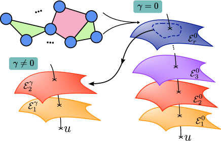
Figure 1: Higher-order decomposition according to the statistical manifold foliation. Dually-flat model (right), and its deformed counterpart (bottom left). The space of MEP distributions with constraints of different orders constitute nested sub-manifolds [25], giving rise to a hierarchy of families of models of the form $\mathcal{E}_{k}^{\gamma}=\{p_{\gamma}^{(k)}(\bm{x})=e^{-\varphi_{\gamma}}\big{[}1-\gamma\beta E_{k}(\bm{x})\big{]}_{+}^{1/\gamma}\}$ such that $\mathcal{E}_{1}^{\gamma}\subset\mathcal{E}_{2}^{\gamma}\subset\dots\subset\mathcal{E}_{n}^{\gamma}$ [32]. The foliation strongly depends on the curvature $\gamma$, and in general $\mathcal{E}_{k}^{\gamma}\neq\mathcal{E}_{k}^{0}$ but rather $\mathcal{E}_{k}^{\gamma}\cap\mathcal{E}_{r}^{0}\neq\varnothing$ for $k<r$. For small values of $|\gamma|$, it is possible to neglect higher-order terms in (4), and therefore subsets of $\mathcal{E}_{k}^{\gamma}$ effectively approximate $\mathcal{E}_{r}^{0}$.

I.2 Curved neural networks

Several well-known neural network models adhere to the MEP, such as Ising-like models [37] and Boltzmann machines [38]. Interestingly, these models can encode patterns in their weights (conforming ‘associative memories’ or Nakano-Amari-Hopfield networks [39, 40, 41]), making them amenable to being extensively studied using tools from equilibrium and nonequilibrium statistical physics literature [42, 43, 44, 45]. Following the principles in the previous section, here we introduce a family of recurrent neural networks that we call curved neural networks.

We consider $N$ binary variables $x_{1},\dots,x_{N}$ taking values in $\{1,-1\}$ following a joint probability distribution

$$p_{\gamma}(\bm{x}) =\exp\left(-\varphi_{\gamma}\right)\big{[}1-\gamma\beta E(\bm{x})\big{]}_{+}^{1/\gamma},$$ (5)

where $\varphi_{\gamma}$ is a normalising constant. Above, we call $E(\bm{x})$ and $\beta$ the energy function and the inverse temperature due to their similarity with the Gibbs distribution in statistical physics when $\gamma\to 0$. Neural networks are typically defined by an energy function

$$E(\bm{x})=-\sum_{i=1}^{N}H_{i}x_{i}-\frac{1}{N}\sum_{i<j}J_{ij}x_{i}x_{j},$$ (6)

where $J_{ij}$ is the coupling strength between $x_{i}$ and $x_{j}$ and $H_{i}$ are bias terms. The limit $\gamma\rightarrow 0$ recovers the Ising model. Emulating classical associative memories, the weights $J_{ij}$ can be made to encode a collection of $M$ neural patterns $\bm{\xi}^{a}=\{\xi_{1}^{a},\dots\xi_{N}^{a}\}$, $\xi_{1}^{a}=\pm 1$ and $a=1,\dots,M$ by using the well-known Hebbian rule [41, 42]

$$J_{ij}=\sum_{a=1}^{M}\xi_{i}^{a}\xi_{j}^{a}.$$ (7)

Before proceeding with our main analysis, one can gain insights about the effect of the curvature $\gamma$ from the dynamics of a recurrent neural network that behaves as a sampler of the equilibrium distribution described by (5). For this, we adapt the classic Glauber dynamics to curved neural networks (see Supplementary Note 2) to obtain

$$p(x_{i}|\bm{x}_{\backslash i}) =\left(1+\left[1+\gamma\beta^{\prime}(\bm{x})\Delta E(\bm{x})\right]_{+}^{1/\gamma}\right)^{-1},$$ (8)

where $\Delta E(\bm{x})=2x_{i}\sum_{j}J_{ij}x_{j}$ is the energy difference associated with detailed balance, and $\beta^{\prime}(\bm{x})$ is an effective inverse temperature given by

$$\beta^{\prime}(\bm{x}) =\frac{\beta}{\left[1-\gamma\beta E(\bm{x})\right]_{+}}.$$ (9)

Again, $\gamma\to 0$ recovers $\beta^{\prime}(\bm{x})=\beta$ and the classical dynamics.

Thus, the curvature affects the dynamics through the deformed nonlinear activation function (8) and the state-dependent effective temperature $\beta^{\prime}(\bm{x})$ (9), with high or low $\beta^{\prime}(\bm{x})$ inducing higher or lower degrees of randomness in the transitions. The effect of $E(\bm{x})$ on $\beta^{\prime}(\bm{x})$ depends then on the sign of $\gamma$. Negative $\gamma$ increases effective temperature during relaxation, creating a positive feedback loop that accelerates convergence to low-energy state. The effect is similar to simulated annealing, but the coupling of the energy and effective temperature let the annealing scheduling to self-regulate. In contrast, positive $\gamma$ decelerates the dynamics through negative feedback. Such accelerating or decelerating dynamics underlie non-trivial complex collective behaviours, which will be examined in the subsequent sections.

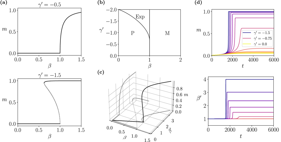
Figure 2: Explosive phase transitions in curved neural networks. (a) Phase transitions of the curved neural network with one associative memory, for values of $\gamma^{\prime}=-0.5$ (top, displaying a second-order phase transition) and $\gamma^{\prime}=-1.5$ (bottom, displaying an explosive phase transition). Solid lines represent the stable fixed points, and dotted lines correspond to unstable fixed points. (b) Phase diagram of the system. The areas indicated by ‘P’ and ‘M’ refer to the usual paramagnetic (disordered) and magnetic (ordered) phases, respectively. The area indicated by ‘Exp’ represents a phase where ordered and disordered states coexist in an explosive phase transition characterised by a hysteresis loop. (c) Solution of Eqs. (15)-(16) for $\beta^{\prime},m,\beta$ (black line) for $\gamma^{\prime}=-1.2$, and projections to the plane $m=0$, $\beta=0$ and $\beta^{\prime}=0$, obtaining respectively the relation between $\beta,\beta^{\prime}$ and solutions of the flat and the deformed models respectively (grey lines). (d) Mean-field dynamics of the single-pattern neural network for $\beta=1.001$ (near criticality from the ordered phase) for some values of $\gamma^{\prime}$ in $[-1.5,0]$. For large negative $\gamma^{\prime}$ the dynamics ‘explodes’, with $m$ (top) and $\beta^{\prime}$ (bottom) converging abruptly.

II Mean-field behaviour of curved associative-memory networks

II.1 Mean-field solution

As with regular associative memories [44], one can solve the behaviour of curved associative-memory networks through mean-field methods in the thermodynamic limit $N\to\infty$ (Supplementary Note 3). Here the energy value of the model is extensive, meaning that it scales with the system’s size $N$. To ensure the deformation parameter remains independent of system properties such as size or temperature, we scale it as follows:

$$\gamma=\frac{\gamma^{\prime}}{N\beta}.$$ (10)

Under this condition, we calculate the normalising potential $\varphi_{\gamma}$ by introducing a delta integral and calculating a saddle-node solution, resulting in a set of order parameters $\bm{m}=\{m_{1},\ldots,m_{M}\}$, $m=\frac{1}{N}\sum_{i}\xi_{i}\left\langle x_{i}\right\rangle$ in the limit of size $N\to\infty$. This calculation assumes $1-\gamma\beta E(\bm{x})>0$ so that $\left[\,\right]_{+}$ operators can be omitted and $\varphi_{\gamma}$ is differentiable. The solution results in (for $H_{i}=0$):

$$\varphi_{\gamma} =N\frac{\beta}{\gamma^{\prime}}\log\frac{\beta^{\prime}}{\beta}-\sum_{a=1}^{M}\beta^{\prime}Nm_{a}^{2}$$

$$\,\quad+\sum_{i=1}^{N}\log\left(2\cosh\left(\beta^{\prime}\sum_{a=1}^{M}\xi_{i}^{a}m_{a}\right)\right),$$ (11)

where $\beta^{\prime}$ is given by

$$\beta^{\prime} =\frac{\beta}{1+\gamma^{\prime}\frac{1}{2}\sum_{a}m_{a}^{2}},$$ (12)

and the values of the mean-field variables $m_{a}$ are found from the following self-consistent equations:

$$m_{a} =\sum_{i=1}^{N}\frac{\xi_{i}^{a}}{N}\tanh\left(\beta^{\prime}\sum_{b=1}^{M}\xi_{i}^{b}m_{b}\right).$$ (13)

Similarly, using a generating functional approach [45], we use the Glauber rule in (8) to derive a dynamical mean-field given by path integral methods (see Supplementary Note 2). This yields

$$\dot{m}_{a} =-m_{a}+\sum_{i=1}^{N}\frac{\xi_{i}^{a}}{N}\tanh\left(\beta^{\prime}\sum_{b=1}^{M}\xi_{i}^{b}m_{b}\right),$$ (14)

where $\beta^{\prime}$ is defined as in (12) for each $\bm{m}$. Note that in the large systems, we recover the classical nonlinear activation function, and the deformation affects the dynamics only through the effective temperature $\beta^{\prime}$.

II.2 Explosive phase transitions

To illustrate these findings, let us focus on a neural network with a single associative pattern ($M=1$), equivalent to a homogeneous mean-field Ising model [46] (with energy $E(\bm{x})=\frac{1}{N}J\sum_{i<j}x_{i}x_{j}$) by using a variable change $x_{i}\leftarrow\xi_{i}x_{i}$. Rewriting (13), we find that a one-pattern curved neural network follows a mean-field model:

$$m =\tanh\left(\beta^{\prime}m\right),$$ (15)

$$\beta^{\prime} =\frac{\beta}{1+\gamma^{\prime}\frac{1}{2}m^{2}}.$$ (16)

This result generalises the well-known Ising mean-field solution $m=\tanh\left(\beta Jm\right)$ for $\gamma=0$.

By evaluating these equations, one finds that the model exhibits the usual order-disorder phase transition for positive and small negative values of $\gamma^{\prime}$. However, for large negative values of $\gamma^{\prime}$, a different behaviour emerges: an explosive phase transition [8] that displays hysteresis due to HOIs (see Fig. 2.a). The resulting phase diagram closely resembles phase transitions in higher-order contagion models [9, 11] and higher-order synchronisation observed in Kuramoto models [26].

Interpretation of the deformation parameter.

One can intuitively interpret the effect of the deformation parameter $\gamma^{\prime}$ by noticing that, for a fixed $\beta^{\prime}$, $m$ is the solution of a function of $\beta^{\prime}$. For $\gamma^{\prime}=0$, this results into the behaviour of the mean-field of the regular exponential model, which assigns a value of $m$ to each inverse temperature $\beta=\beta^{\prime}$. In the case of the deformed model, the possible pairs of solutions $(m,\beta^{\prime})$ are the same, but it changes their mapping to the inverse temperatures $\beta$. Namely, this deformation can be interpreted as a stretching (or contraction) of the effective temperature, which maps each pair $(m,\beta^{\prime})$ to an inverse temperature $\beta=\beta^{\prime}(1+\frac{1}{2}\gamma^{\prime}Jm^{2})$ according to (16). Thus, one can obtain the mean-field solutions of the deformed patterns as mappings of the solutions of the original model. This is illustrated in Fig. 2.c, where the solution of $\beta^{\prime},m,\beta$ is projected to the planes $\beta=0$ and $\beta^{\prime}=0$, obtaining the solutions of the flat ($\gamma^{\prime}=0$) and the deformed ($\gamma^{\prime}=-1.2$) models respectively.

Explosive dynamics.

In order to gain a deeper understanding of the explosive nature of this phase transition, we study the dynamics of the single-pattern neural network. Rewriting (14) for $M=1$ and under the change of variables above to remove $\bm{\xi}$, the dynamical mean-field equation of the system reduces to

$$\dot{m}=-m+\tanh\left(\beta^{\prime}m\right),$$ (17)

where $\beta^{\prime}$ is calculated as in (16). Simulations of the dynamical mean-field equations for values of $\beta$ just above the critical point are depicted in Fig. 2.d. Trajectories with strongly negative $\gamma^{\prime}$ saturate earlier than smaller negative $\gamma^{\prime}$, confirming accelerated convergence. During this process, the effective inverse temperature $\beta^{\prime}$ rapidly increases until it saturates, making the dynamics more deterministic. More deterministic dynamics lead to faster convergence of $m$, which in turn increases $\beta^{\prime}$, creating a positive feedback loop between $\beta^{\prime}$ and $m$ that gives rises to the explosive nature of the phase transition. This positive loop occurs only if $\gamma^{\prime}$ is negative; otherwise, negative feedback simply makes the convergence of $m$ slower.

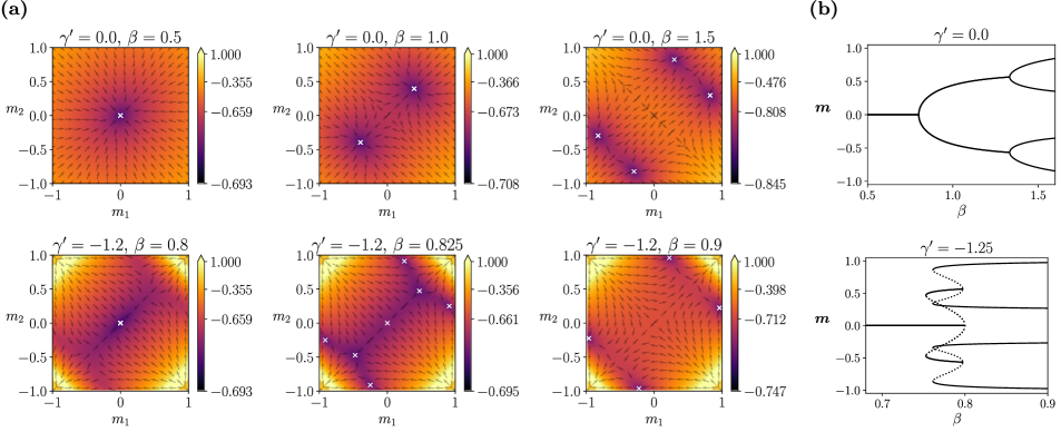
Figure 3: Interaction between two encoded memories. (a) Values of $\varphi_{\gamma}$ for different mean-field values $m_{1},m_{2}$, indicating the attractor structure of the network for different values of $\beta$ with $C=0.2$ for $\gamma^{\prime}=0$ (top row) and $\gamma^{\prime}=-1.2$ (bottom row). (b) Bifurcations of the order parameters $m_{1},m_{2}$. For $\gamma^{\prime}=0$ we observe an attractor bifurcating into two and then into four. For $\gamma^{\prime}=-1.2$, we observe the same sequence, but with a coexistence hysteresis regime in which 7 attractors are possible.

II.3 Overlaps between memory basins of attraction

A key property of associative-memory networks is their ability to retrieve patterns in different contexts. In one-pattern associative-memory networks, energy $E(\bm{x})=-\sum_{i<j}x_{i}\xi_{i}\xi_{j}x_{j}$ is a quadratic function with two minima at $\bm{x}=\pm\bm{\xi}$, which act as global attractors. Instead, a two-pattern associative-memory network has an energy function with four minima (if sufficiently separated), but their attraction basins overlap when the patterns are correlated. Dense associative memories enhance their memory capacity by narrowing the basins of attraction through a highly nonlinear energy function [20, 21].

To study the degree of the overlap between pairs of patterns, we analyse solutions of (13) for a network with two patterns with correlation $\left\langle\xi_{i}^{1}\xi_{i}^{2}\right\rangle=C$ (see Supplementary Note 3.3 for details). The system is in this case described by two mean field patterns

$$m_{a} =\frac{1}{2}(1+C)\tanh\left(\beta^{\prime}(m_{1}+m_{2})\right)$$

$$\,\quad+w\frac{1}{2}(1-C)\tanh\left(\beta^{\prime}(m_{1}-m_{2})\right),$$ (18)

with $w=3-2a=\pm 1$ for $a=1,2$ and

$$\beta^{\prime} =\frac{\beta}{1+\gamma\frac{1}{2}(m_{1}^{2}+m_{2}^{2})}.$$ (19)

Fig. 3 shows how the hysteresis effect is linked to explosive phase transitions persists in the case of two patterns for $C=0.2$. Additionally, the explosive region spans two consecutive bifurcations (going from 1 to 2, and then to 4 fixed points), creating a hysteresis cycle involving 7 fixed points. This illustrates embedded hysteresis cycles, as well as an increased memory capacity for finite temperatures. This intriguing enhanced capability for memory retrieval is further investigated by the analyses presented in the next section.

III Memory retrieval with an extensive number of patterns

Next, we sought to investigate how the deformation related to $\gamma$ impacts the memory-storage capacity of associative memories. In classical associative networks of $N$ neurons, taking $M=\alpha N$ as the number of patterns learned by the network transforms the system into a disordered spin model in the thermodynamic limit. Furthermore, using the replica-trick method, one can analytically solve this model to determine its memory capacity [47], and theoretically identify the critical value of $\alpha$ at which memory retrieval becomes impossible — leading to a disordered spin-glass phase. Here, we apply a similar approach to reveal how deformed associative memory networks afford an enhanced memory capacity.

Applying the replica trick in conjunction with the methods outlined in previous sections allows us to solve the system using $\varphi_{\gamma}$ for the deformed exponential (see Supplementary Note 5). This method entails computing a mean-field variable $m$ corresponding to one of the patterns $\bm{\xi}^{a}$ and averaging over the others. For simplicity, a pattern with all positive unity values $\bm{\xi}^{a}=(1,1,\ldots,1)$ is considered, which is equivalent to any other single pattern just by a series of sign flip variable changes. The resulting averaged activity across other patterns introduces a new order parameter $q$, contributing to disorder in the system. After introducing the relevant order parameters and solving under a replica-symmetry assumption, the normalising potential is derived as

$$\varphi_{\gamma} =N\frac{\beta}{\gamma^{\prime}}\log{\frac{\beta}{\beta^{\prime}}}-N\beta^{\prime}Jm^{2}-N\frac{1}{2}\alpha(\beta^{\prime}J)^{2}(r+R-2qr)$$

$$\,\quad-N\frac{1}{2}\alpha\left(\log\left(1-\beta^{\prime}J(1-q)\right)-\beta^{\prime}J\sqrt{rq}\right)$$

$$\,\quad+N\int Dz\log\left(2\cosh\left(\beta^{\prime}Jm+\beta^{\prime}J\sqrt{\alpha r}z\right)\right),$$ (20)

where $J$ is a scaling factor and order parameters are defined as

$$m =\int Dz\tanh\left(\beta^{\prime}Jm+\beta^{\prime}J\sqrt{\alpha r}z\right),$$ (21)

$$q =\int Dz\tanh^{2}\left(\beta^{\prime}Jm+\beta^{\prime}J\sqrt{\alpha r}z\right),$$ (22)

with

$$r=\frac{q}{(1-\beta^{\prime}J(1-q))^{2}},\quad R=\frac{(\beta^{\prime}J)^{-1}-(1-2q)}{(1-\beta^{\prime}J(1-q))^{2}}.$$ (23)

As in previous cases, the model is governed by an effective temperature

$$\beta^{\prime} =\frac{\beta}{1+\gamma^{\prime}\frac{1}{2}\left(Jm^{2}+\alpha J(\beta^{\prime}(R-qr)-1)\right)}.$$ (24)

This solution differs from the models in previous sections by the self-dependence of $\beta^{\prime}$.

By solving Equations (21-22) across different values of $\alpha$ and $\gamma^{\prime}$, one can construct the phase diagram of the system. Fig. 4.a shows three distinct phases for $\beta=2$:

• A ferromagnetic phase (F) corresponds to stable solutions with $m>0$, corresponding to memory retrieval.

• A spin-glass phase exhibits solutions where $m=0$ and $q>0$.

• A mixed phase (M) where both types of solutions coexist, being the spin-glass phase a global minimum of the free-energy.

Note that expansion of the ferromagnetic phase with negative $\gamma^{\prime}$ indicates enhanced memory-storage capacity by the HOIs. In the mixed phase, memory retrieval presents a local — but not global — minimum of the normalising potential $\varphi_{\gamma}$ in (20). For $\gamma^{\prime}=0$, the phase transition reflects the behaviour of associative memories near saturation [47, 44].

The stability of the replica symmetry solution is given by the condition

$$(1+\beta^{\prime}(1-q))^{2}>\alpha\beta^{\prime 2}\int Dz\cosh^{-4}\beta^{\prime}\left(Jm+J\sqrt{\alpha r}z\right).$$ (25)

Solving the equation numerically we observe that the spin glass solutions remain unstable under the replica symmetry assumption, indicating replica symmetry breaking effects. However, the memory retrieval solutions in F and M are stable for all values of $\alpha,\gamma^{\prime}$ for $\beta=2$, indicating that the memory capacity calculation is correct under replica symmetric assumptions.

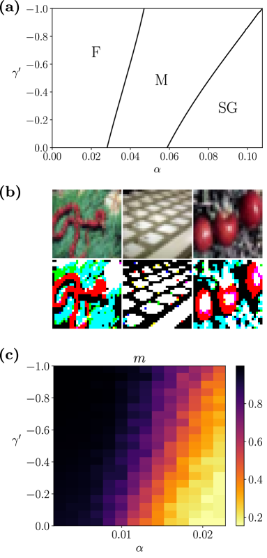
Figure 4: Memory capacity is enhanced by geometric deformation. (a) Phase diagram of a model with an extensive number of patterns $M=\alpha N$ for $\beta=2$, where F indicates the ferromagnetic (i.e., memory retrieval) phase, SG the spin-glass phase (where saturation makes memory retrieval inviable) and M a mixed phase where the two coexist. Increasing $\gamma^{\prime}$ to larger negative values extends the retrieval phase into larger values of $\alpha$, indicating an increased memory capacity. (b) Examples of CIFAR-100 images (top) and their RGB binarised versions (bottom). Every 32x32x3 binary RGB pixel value for each image $a$ is assigned to the value of one position of pattern $\xi_{i}^{a}$. (c) Average pattern retrieval obtained in experiments, measured by the overlap between the final state of the network and the correct pattern.

Experimental validation

We complement the analysis from the previous section with an experimental study of a system encoding patterns from an image-classification benchmark. The patterns are sourced from the CIFAR-100 dataset, which comprises $60,000$ 32x32 colour images [48]. To adapt the dataset to binary patterns suitable for storage in an associative memory, we processed each RGB channel by assigning a value of $1$ to pixels with values greater than the channel’s median value and $-1$ otherwise (Fig. 4.b). The resulting array of $N=32\cdot 32\cdot 3$ binary values for each image was assigned to patterns $\bm{\xi}^{a}$. Note that associative memories (as well as our theory above) usually assume that patterns are relatively uncorrelated. Thus, our experiments used a selection of 100 images whose covariance values were smaller than $10/\sqrt{N}$ (covariance values of uncorrelated patterns have a standard deviation of $1/\sqrt{N}$).

We evaluate the memory retrieval capacity of networks with various degrees of curvature $\gamma$ by encoding different numbers of memories, as described in (7). As a measure of performance, we evaluated the stability of the network by assigning an initial state $\bm{x}=\bm{\xi}^{a}$ and calculating the overlap $o_{a}=\sum_{i}x_{i}\xi_{i}^{a}$ after $T=30N$ Glauber updates. The process was repeated $R=500$ times from different initial conditions to estimate the value of $m$ in (21). Experimental outcomes confirm our theoretical results, revealing that memory capacity increases with negative values of $\gamma^{\prime}$ (see Fig. 4.c). Note that the resulting memory capacity of the system observed in our experiments (i.e., the value of $\alpha$ at which the transition happens) is diminished due to the presence of correlations among some of the memorised patterns.

Explosive spin-glass transition

For $J\to 0$ and $\alpha=J^{-2}$, the model converges to (see Supplementary Note 5)

$$q =\int Dz\tanh^{2}\left(\beta^{\prime}\sqrt{q}z\right),$$ (26)

$$\beta^{\prime} =\frac{\beta}{1+\frac{1}{2}\gamma^{\prime}\beta^{\prime}(1-q^{2})},$$ (27)

which at $\gamma=0$ recovers the well-known Sherrington-Kirkpatric model [49]. While in the classical case a phase transition occurs from a paramagnetic to a spin-glass phase, the curvature effect of $\gamma^{\prime}\neq 0$ introduces novel phase transitions. For small values of $\gamma^{\prime}$, the system exhibits a continuous phase transition akin to the Sherrington-Kirkpatrick spin-glass, where $\frac{dq}{d\beta}$ shows a cusp (Fig. 5.a). However, for $\gamma^{\prime}=-1$ the phase transition becomes second-order, displaying a divergence of $\frac{dq}{d\beta}$ at the critical point (Fig. 5.b). Moreover, increasing the magnitude of negative $\gamma^{\prime}$ leads to a first-order phase transition with hysteresis (Fig. 5.c), resembling the explosive phase transition observed in the single-pattern associative-memory network. This hybrid phase transition combines the typical critical divergence of a second-order phase transition with a genuine discontinuity, similar to ‘type V’ transitions as described in [8].

We analytically calculated the properties of these phase transitions (see Supplementary Note 6). By computing the solution at $\gamma^{\prime}=0$ and rescaling $\beta^{\prime}$, we determined that the critical point is located at $\beta_{c}=1+\frac{1}{2}\gamma^{\prime}$ (consistent with Fig. 5.a-c). The slope of the order parameter around the critical point is, for $\gamma^{\prime}<1$, equal to $(1+\gamma^{\prime})^{-1}$, indicating the onset of a second-order phase transition as depicted in Fig. 5.b. The resulting phase diagram of the curved Sherrington-Kirkpatrick model is shown in Fig. 5.d.

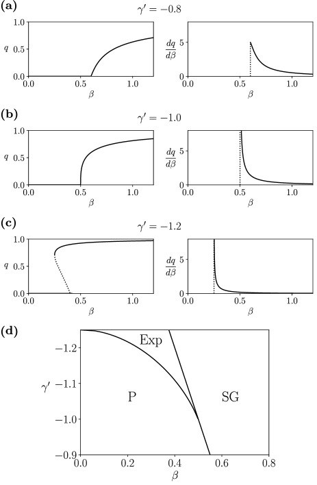
Figure 5: Explosive spin glasses. Phase transitions for order parameter $q$ for replica-symmetric disordered spin models displaying (a) a cusp phase transition for $\gamma^{\prime}=-0.5$, , (b) a second-order phase transition for $\gamma^{\prime}=-1.0$ and (c) an explosive phase transition for $\gamma^{\prime}=-1.2$. (d) Phase diagram of the explosive spin glass, displaying a paramagnetic (‘P’), spin-glass (‘SG’) and an explosive phase (‘Exp’).

IV Future directions for the study of higher-order interactions

HOIs play a critical role in enabling emergent collective phenomena in biological and artificial systems, supporting complex behaviour across a wide range of disciplines. Modelling HOIs is, however, highly non-trivial, often requiring advanced analytic tools (such as hypergraphs and simplicial complexes) that entail an exponential increase in parameters for large systems. Here, we address this issue by leveraging an information-geometric generalisation of the maximum entropy principle, effectively capturing HOIs in models via a deformation parameter $\gamma$ associated with the Rényi entropy parameter. Given their close connection with statistical physics, this family of models provides an ideal setup to investigate the effect of HOIs on collective phenomena, including phase transitions and the capability of networks to store memories.

Our results demonstrate how HOIs accelerate dynamics through a feedback loop between the energy and an effective temperature. This feedback loop can cause explosive phase transitions in the average activity rate and other complex phenomena such as explosive spin glass transitions. Specifically, this loop can either accelerate (for negative $\gamma$ values) or decelerate (for positive $\gamma$ values) the model’s convergence, which is recognised as a key mechanism behind explosive phase transitions [7, 9, 11, 2, 8]. Our results offer a family of models amenable for analytical study to investigate explosive phenomena in neural networks, which constitutes an unexplored topic. Additionally, they provide a theoretical explanation for the emergence of explosive behaviour in connection with Rényi/Tsallis entropy and curved statistical manifolds.

Our findings also reveal that HOIs can increase the memory capacity of associative-memory networks. Negative values of the deformation parameter $\gamma$ increase the memory capacity of associative-memory networks. These findings align with the observations that memory capacity is enhanced by introducing high-order nonlinearities in energy functions in recurrent neural networks [20, 21] and related state-of-the-art architectures like transformers [22]. However, it is worth noticing that these models use an approach different from the deformation of the statistical manifolds, as they apply non-linearities individually to each encoded pattern in a way to narrow each memory’s basin of attraction and prevent the spin-glass phase. By using this method, dense associative memories display supralinear (e.g. polynomial or exponential) memory capacities [20, 21]. In our setup, we aimed for a parsimonious framework rather than maximising memory capacity, but combining both approaches to enhance memory capacity would be an interesting line of future research.

Our results demonstrate the benefits of considering entropy measures, emergent HOIs, and nonlinear network dynamics as theoretically intertwined notions. As showcased here, such an integrated framework reveals how information encoding, retrieval dynamics, and memory capacity in artificial neural networks are mediated by HOIs, providing principled, analytically tractable tools and insights from statistical mechanics and nonlinear dynamics. This approach could also be applied to biological neural systems, where evidence suggests the presence of alternating positive and negative high-order interactions, resulting in sparse neuronal activity that allows for long periods of total silence [14, 13, 15, 5]. Future work may explore information coding of biological neurons realising such structured HOIs, e.g., by incorporating the effect of a negative bias term in the model. More generally, the framework presented in this paper extends beyond neural networks and contributes to a general theory of HOIs, paving a route towards a principled study of higher-order phenomena in complex networks.

Contributions

M.A., P.A.M, F.E.R and H.S. designed and reviewed the research and wrote the paper. M.A. contributed the analytical and numerical results. P.A.M. contributed part of the analytical results in Section III.

Supplementary Note 1 Maximum Rényi entropy and Information Geometry

The maximum entropy principle (MEP) is a framework for building parsimonious models consistent with observations, being particularly well-suited for the statistical description of systems in contexts of incomplete knowledge [28, 29]. The MEP uses entropy as a fundamental tool to quantify the degree of structure present in a given model. Accordingly, the MEP suggest to adopt the model with the maximal entropy — i.e. the least amount of structure — that is compatible with a given set of observations, following the idea that one should not include regularities that are not contained in the data.

Maximum entropy models are particularly well-suited for the study of neural systems. By abstracting neurons into binary variables $x_{k}$ representing the presence or absence of action potentials, the MEP provides a powerful approach to model collective neural activity. In this approach, the Ising model emerges from the maximisation of Shannon entropy under constraints on activity rates of individual neurons and pairwise correlations:

$$p^{(2)}=\operatorname*{arg\,max}_{q(\bm{x})}H(\bm{x})\quad\text{s.t.}\quad\begin{cases}\left\langle x_{i}\right\rangle&=\eta_{i},\\ \left\langle x_{i}x_{j}\right\rangle&=\eta_{ij},\end{cases}$$

where $H(\bm{x})$ denotes the Shannon entropy of $\bm{x}=(x_{1},\dots,x_{n})$ under distribution $q(\bm{x})$. It can be shown that

$$p^{(2)}(\bm{x})=\frac{1}{Z}\exp\left(\sum_{i}\theta_{i}x_{i}+\sum_{i<j}\theta_{ij}x_{i}x_{j}\right),$$ (S1.28)

with $Z$ being a normalising constant. Hence, this model encapsulates observed information up to second-order statistics, represented in how $\theta_{i},\theta_{ij}$ depend on the constraints $\eta_{i},\eta_{ij}$. Furthermore, the dynamics of the Ising model can be investigated via exact solutions, approximations (encompassing mean-field and Bethe approximations), and simulations, thereby providing a rich set of insights and analytical tools. The Ising model has been instrumental in the development of recurrent neural networks, leading to Hopfield networks and Boltzmann machines.

What if the observations that one is to model require us to consider statistics beyond pairwise interactions? Following the same principle, one can construct models with third- and higher-order interactions [25] resulting on distributions of the following type:

$$p^{(k)}(\bm{x})=\frac{1}{Z}\exp\bBigg@{3}(\sum_{\begin{subarray}{c}\bm{I}\subseteq\{1,\dots,n\}\\ |\bm{I}|\leq k\end{subarray}}\theta_{\bm{I}}\prod_{i\in\bm{I}}x_{i}\bBigg@{3})$$ (S1.29)

with the summation going over all subsets of $k$ or less variables. Above, the argument within the exponential is an energy function $E_{k}(\bm{x})$, with the index $k$ highlighting the highest order of interactions considered. It is important to notice that the number of terms in the Hamiltonian grows exponentially with $k$, making unfeasible in practice to construct models including high orders $k\gg 1$.

1.1 Capturing high-order interactions via non-Shannon entropies

While traditional formulations of the MEP are based on Shannon’s entropy [30], more recent work has expanded it to include other entropy functionals including the entropies of Tsallis [31] and Rényi [32]. Here we argue that some high-order interdependencies can be efficiently captured by the deformed exponential family (2), which arises as a solution to the problem of maximising non-Shannon entropies — as explained below.

By starting from a conventional MEP model with few degrees of freedom tuned to account for low-order interactions, one can enhance its capability to account for higher-order interdependencies by the inclusion of a deformation parameter, defined as a continuum extension of the Rényi’s index (or Tsallis’s $\alpha$), with clear geometrical interpretation, i.e. the scalar curvature of the manifold. Concretely, let’s consider the Rényi entropy with parameter $\gamma\geq-1$, given by

$$H_{\gamma}=-\frac{1}{\gamma}\log\sum_{\bm{x}}p(\bm{x})^{1+\gamma}.$$ (S1.30)

This definition adopts the shifted indexing convention introduced in Ref. [33], thereby referring to $\gamma=n-1$ as the order of Rényi’s entropy, with $n\geq 0$ corresponding to the order in the standard definition. Rényi entropy recovers the standard Shannon entropy at the limit $\gamma\to 0$. The maximisation of the Rényi entropy can be performed by extremisation of the Lagrangian:

$$\mathcal{L} =-\frac{1}{\gamma}\log\sum_{\bm{x}}p(\bm{x})^{1+\gamma}+\theta_{0}\left(\sum_{\bm{x}}p(\bm{x})-1\right)+\theta_{0}\gamma\beta\sum_{i=1}^{L}\theta_{i}\left(\sum_{\bm{x}}p(\bm{x})f_{i}(\bm{x})-c_{i}\right),$$ (S1.31)

which also consider constraints $\sum_{\bm{x}}p(\bm{x})=1$ and $\sum_{\bm{x}}p(\bm{x})f_{i}(\bm{x})=k_{i}$ with $i=1,\dots,L$, whereas the first ensures $p(\bm{x})$ to be a probability mass function and the second fixes the average of $f_{i}(\bm{x})$ on a desired value $c_{i}$. Note that the coefficient $\beta$ is introduced to keep $\gamma$ dimensionless, corresponding to the inverse temperature in statistical physics. This results into the maximum entropy condition

$$0=\frac{\delta\mathcal{L}}{\delta p(\bm{x})}=-\frac{1}{\gamma}\frac{(1+\gamma)p(\bm{x})^{\gamma}}{\sum_{\bm{x}}p(\bm{x})^{1+\gamma}}+\theta_{0}+\theta_{0}\gamma\beta\sum_{a}\theta_{a}f_{a}(\bm{x}).$$ (S1.32)

The family of probability distributions meeting the above condition is known as the deformed exponential family, which is given by

$$p_{\gamma}(\bm{x})=\exp(-\varphi_{\gamma})\bigg{[}1+\gamma\beta\sum_{a}\theta_{a}f_{a}(\bm{x})\bigg{]}_{+}^{1/\gamma}$$ (S1.33)

where $\varphi_{\gamma}$ is a normalising constant

$$\varphi_{\gamma}=\log\sum_{\bm{x}}\bigg{[}1+\gamma\beta\sum_{a}\theta_{a}f_{a}(\bm{x})\bigg{]}_{+}^{1/\gamma}.$$ (S1.34)

Above, we use the square bracket $\left[\cdot\right]_{+}$ operator to sets negative values to zero, so that $\left[x\right]_{+}=\max\{0,x\}$. In the next sections, to solve the steepest descent step of mean field calculations, we will assume that the content of the $\left[\cdot\right]_{+}$ operator is always possible, so differentiation is always positive. This assumption is reasonable under an adequate normalisation of $\gamma$.

Importantly, Renyi’s entropy is closely related to Tsallis’ entropy

$$H_{\gamma}^{(\mathrm{Ts})}=-\frac{1}{\gamma}\left(1-\sum_{\bm{x}}p(\bm{x})^{1+\gamma}\right).$$ (S1.35)

It can be shown that the Tsallis and Rényi’s entropies can be deformed into one another by a monotonically increasing function. This fact brings both divergences, from the geometrical perspective, to the same equivalence class generating the same geometry, see Ref. [32]. In particular, by maximising Tsallis entropy one recovers the same deformed exponential family, $p_{\gamma}$ using $q=1-\gamma$ [34].

Supplementary Note 2 Glauber rule

Glauber dynamics is a Markov Chain Monte Carlo algorithm that is popular for simulating neural activity according to Hopfield networks and Ising models. In this method, one samples the activity of each neurons conditioned on the activity of other neurons according to the following conditional distribution:

$$p_{\gamma}(x_{k}|\bm{x}_{\backslash k}) =\frac{p_{\gamma}(x_{k},\bm{x}_{\backslash k})}{p_{\gamma}(\bm{x}_{\setminus k})}=\frac{p_{\gamma}(x_{k},\bm{x}_{\backslash k})}{p_{\gamma}(x_{k},\bm{x}_{\backslash k})+p_{\gamma}(-x_{k},\bm{x}_{\backslash k})},$$ (S2.36)

where $\bm{x}_{\backslash k}$ denotes the state of all neurons expect the $k$-th one. This sampling procedure is carried out for all neurons in an iterative manner.

Let us construct Glauber dynamics for a curved neural network. The deformed exponential family distribution states that the distribution of $\bm{x}$ is given by

$$p_{\gamma}(\bm{x}) =\exp\left(-\varphi_{\gamma}\right)\left[1-\gamma\beta E(\bm{x})\right]_{+}^{1/\gamma},$$ (S2.37)

where the energy function $E(\bm{x})$ is given by

$$E(\bm{x}) =-\sum_{i}H_{i}x_{i}-\frac{1}{2N}\sum_{i,j}J_{ij}x_{i}x_{j}.$$ (S2.38)

The deformed exponential family distribution can be rewritten as

$$p_{\gamma}(-x_{k},\bm{x}_{\backslash k})=\exp\left(-\varphi\right)\left[1-\gamma\beta\left(E(\bm{x})-2x_{i}h_{i}\right)\right]_{+}^{1/\gamma},$$ (S2.39)

with $h_{i}=H_{i}+\sum_{j}J_{ij}x_{j}$. Under the assumption of $1-\gamma\beta E(\bm{x})>0$ (and the same for the state resulting from flipping the $k$-th spin), a direct derivation shows that

$$p_{\gamma}(x_{k}|\bm{x}_{\backslash k}) =\frac{\left(1-\gamma\beta E(\bm{x})\right)^{1/\gamma}}{\left(1-\gamma\beta E(\bm{x})\right)^{1/\gamma}+\left(1-\gamma\beta\left(E(\bm{x})-2x_{k}h_{k}\right)\right)^{1/\gamma}}$$

$$=\left(1+\left(\frac{1-\gamma\beta\left(E(\bm{x})-2x_{k}h_{k}\right)}{1-\gamma\beta E(\bm{x})}\right)^{1/\gamma}\right)^{-1}$$

$$=\left(1+\left(1+\gamma 2\beta^{\prime}x_{k}h_{k}\right)^{1/\gamma}\right)^{-1}$$

$$=\left(1+\exp_{\gamma}\left(-2\beta^{\prime}x_{k}h_{k}\right)\right)^{-1}$$ (S2.40)

$$\beta^{\prime} =\frac{\beta}{\left(1-\gamma\beta E(\bm{x})\right)}.$$ (S2.41)

where $\exp_{\gamma}(\cdot)$ stands for the deformed exponential. Note that these equations recover the classical Glauber rule for Ising models at $\gamma=0$. The mean activation rate of the $k$-th neuron conditional on other neurons’ state is then given by

$$\tilde{m}_{k}(\bm{x}) =p_{\gamma}(x_{k}=+1|\mathbf{x}_{\backslash k})-p_{\gamma}(x_{k}=-1|\mathbf{x}_{\backslash k})$$

$$=\frac{1-\exp_{\gamma}\left(-2\beta^{\prime}x_{k}h_{k}\right)}{1+\exp_{\gamma}\left(-2\beta^{\prime}x_{k}h_{k}\right)}.$$ (S2.42)

For implementing the sampling strategy, the selection of neurons can be sequential, using random permutations, or using probabilistic methods (according to non-zero probabilities assigned to each neuron).

In the case of large systems in which $E(\bm{x})$ extensive, then a normalisation of the curvature parameter in the form $\gamma^{\prime}=\frac{\gamma}{N}$ is required. This makes the value of $\gamma x_{k}h_{k}$ to tend to zero as $N\to\infty$. In this case, calculating the limit of $\exp_{\gamma}\left(-2\beta^{\prime}x_{k}h_{k}\right)$ as $\gamma\to 0$, one finds that

$$p_{\gamma}(x_{k}|\bm{x}_{\backslash k}) =\left(1+\exp\left(-2\beta^{\prime}x_{k}h_{k}\right)\right)^{-1}=\frac{\exp\left(\beta^{\prime}x_{k}h_{k}\right)}{\cosh\left(\beta^{\prime}h_{k}\right)},$$ (S2.43)

with effective temperature $\beta^{\prime}$ given by

$$\beta^{\prime} =\frac{\beta}{1-\gamma^{\prime}\frac{1}{N}\beta E(\bm{x})}$$ (S2.44)

and

$$\tilde{m}_{k}(\bm{x}) =\tanh\left(\beta^{\prime}h_{k}\right).$$ (S2.45)

Supplementary Note 3 The mean-field theory of curved neural network

3.1 Derivation of general mean-field solution

In this section we study a curved neural network composed of $N$ neurons that stores $M$ patterns $\bm{\xi}^{a}=(\xi_{1}^{a},\dots,\xi_{N}^{a})$, as described by the deformed exponential family distribution given by

$$p_{\gamma}(\bm{x}) =\exp\left(-\varphi_{\gamma}\right)\Bigg{[}1+\gamma\beta\Bigg{(}H\sum_{a,i}\xi_{i}^{a}x_{i}+\frac{J}{N}\sum_{a,i<j}x_{i}\xi_{i}^{a}\xi_{j}^{a}x_{j}\Bigg{)}\Bigg{]}_{+}^{1/\gamma},$$ (S3.46)

where $\varphi_{\gamma}$ is the normalising potential and $\gamma$ is the deformation parameter. In the following sections we assume that parameters are scaled so to that the content of the brackets $\left[\,\right]_{+}$ is always positive, to avoid non-differentiable values.

We start the analysis by computing the value of $\exp\left(\varphi\right)$ in the large $N$ limit, which can be done employing a delta integral substituting the value of $\frac{1}{N}\sum_{i}x_{i}$:

$$\exp\left(\varphi_{\gamma}\right) =\sum_{\bm{x}}\Bigg{[}1+\gamma\beta\Bigg{(}H\sum_{a,i}\xi_{i}^{a}x_{i}+\frac{J}{N}\sum_{a,i<j}x_{i}\xi_{i}^{a}\xi_{j}^{a}x_{j}\Bigg{)}\Bigg{]}^{1/\gamma}_{+}$$

$$=\sum_{\bm{x}}\exp\left(\frac{1}{\gamma}\log\left(1+\gamma\beta\left(H\sum_{a,i}\xi_{i}^{a}x_{i}+\sum_{a}\frac{J}{2N}\left(\bigg{(}\sum_{i}\xi_{i}^{a}x_{i}\bigg{)}^{2}-N\right)\right)\right)\right),$$ (S3.47)

where the second equality uses $(\sum_{i}z_{i})^{2}-N=2\sum_{i<j}z_{i}z_{j}$. Additionally, by replacing $\frac{1}{N}\sum_{i}\xi_{i}^{a}x_{i}$ by a Dirac delta function under an integral, and then using the delta function’s integral form $\delta\left(x-a\right)=\frac{1}{2\pi}\int_{-\infty}^{\infty}e^{\mathrm{i}\mkern 1.0mu\zeta(x-a)}\,d\zeta$, the expression above can be re-written as

$$\exp\left(\varphi_{\gamma}\right) =\sum_{\bm{x}}\int d\bm{m}\prod_{a}\delta\left(m_{a}-\frac{1}{N}\sum_{i}\xi_{i}^{a}x_{i}\right)\exp\left(\frac{1}{\gamma}\log\left(1+\gamma N\beta\sum_{a}\left(Hm_{a}+\frac{J}{2}\left(m_{a}^{2}-\frac{1}{N}\right)\right)\right)\right)$$

$$=\frac{1}{(2\pi)^{M}}\int d\bm{m}d\bm{\hat{m}}\sum_{\bm{x}}\exp\left(\frac{1}{\gamma}\log\left(1+\gamma N\beta\sum_{a}\left(Hm_{a}+\frac{J}{2}\left(m_{a}^{2}-\frac{1}{N}\right)\right)\right)-\sum_{a}\mathrm{i}\mkern 1.0mu\hat{m}_{a}\bigg{(}m_{a}-\frac{1}{N}\sum_{i}\xi_{i}^{a}x_{i}\bigg{)}\right).$$ (S3.48)

Let us now introduce a scaling rule for the deformation parameter $\gamma$ given by

$$\gamma=\frac{\gamma^{\prime}}{\beta N},$$ (S3.49)

where $\gamma^{\prime}$ is a constant independent of $N$, which is motivated by subsequent results for the mean-field solution that suggest this relationship between $\gamma$ and $N$ in order to maintain scale-invariant properties. Then, the potential $\varphi_{\gamma}$ can be expressed in terms of $\gamma^{\prime}$ as

$$\exp\left(\varphi_{\gamma}\right) =\frac{1}{(2\pi)^{M}}\int d\bm{m}d\bm{\hat{m}}\exp\left(\frac{N\beta}{\gamma^{\prime}}\log\left(1+\gamma^{\prime}\sum_{a}\left(Hm_{a}+\frac{J}{2}\left(m_{a}^{2}-\frac{1}{N}\right)\right)\right)\right.$$

$$\qquad\qquad\qquad\qquad\qquad\qquad\quad\qquad\left.-\sum_{a}\mathrm{i}\mkern 1.0mu\hat{m}_{a}m_{a}+\sum_{i}\log\left(2\cosh\left(\frac{1}{N}\sum_{a}\xi_{i}^{a}\mathrm{i}\mkern 1.0mu\hat{m}_{a}\right)\right)\right).$$ (S3.50)

Under this condition, the exponent in the equation above goes to infinity as $N\to\infty$. In this limit, the integral can be evaluated by the method of the steepest descent (a.k.a. the saddle-point method). By differentiating the exponent by $\hat{m}_{a}$, we find the saddle point must satisfy

$$m_{a}=\frac{1}{N}\sum_{i}\xi_{i}^{a}\tanh\left(\frac{1}{N}\sum_{b}\xi_{i}^{b}\mathrm{i}\mkern 1.0mu\hat{m}_{b}\right).$$ (S3.51)

Similarly, differentiating by $m_{a}$ yields

$$\mathrm{i}\mkern 1.0mu\hat{m}_{a} =\beta^{\prime}N(H+Jm_{a}),$$ (S3.52)

where we introduced the effective inverse temperature $\beta^{\prime}$:

$$\beta^{\prime} =\frac{\beta}{1+\gamma^{\prime}\sum_{b}\left(Hm_{b}+\frac{J}{2}m_{b}^{2}\right)}.$$ (S3.53)

From these equations, we find the mean field solution in the limit of large $N$:

$$m_{a}=\frac{1}{N}\sum_{i}\xi_{i}^{a}\tanh\left(\beta^{\prime}\sum_{b}\xi_{i}^{b}(H+Jm_{b})\right),$$ (S3.54)

which recovers the classical mean field solution at $\gamma^{\prime}=0$. This solution confirms that $\gamma$ has to be scaled by the system size to maintain the scale-invariant properties.

The normalising potential in the large $N$ limit is obtained as

$$\varphi_{\gamma}=\frac{\beta N}{\gamma^{\prime}}\log\frac{\beta^{\prime}}{\beta}-\sum_{a}m_{a}\beta^{\prime}N(H+Jm_{a})+\sum_{i}\log\left(2\cosh\left(\beta^{\prime}\sum_{a}\xi_{i}^{a}(H+Jm_{a})\right)\right).$$ (S3.55)

3.2 A single pattern: explosive phase transitions

When embedded memory contains only a single pattern ($M=1$), the equations above result in

$$\varphi_{\gamma} =\frac{\beta N}{\gamma^{\prime}}\log\frac{\beta^{\prime}}{\beta}-N\beta^{\prime}(H+Jm)m+N\log\left(2\cosh\left(\beta^{\prime}(H+Jm)\right)\right),$$ (S3.56)

with

$$m =\tanh\left(\beta^{\prime}(H+Jm)\right),$$ (S3.57)

$$\beta^{\prime} =\frac{\beta}{1+\gamma^{\prime}(Hm+\frac{J}{2}m^{2})}.$$ (S3.58)

Under the limit of small $\gamma$ given by the scaling Eq. S3.49, the derivative of the normalisation potential $\varphi_{\gamma}$ w.r.t. $H$ yields the corresponding expected value, similarly to the exponential family distribution. Then, $\gamma^{\prime}=0$ yields the classical result. This can be verified by

$$\frac{\partial\varphi_{\gamma}}{\partial H} =-\frac{\beta N}{\gamma^{\prime}}\frac{\partial\beta^{\prime}}{\partial H}-N\beta^{\prime}(H+Jm)\frac{\partial m}{\partial H}-N\frac{\partial\beta^{\prime}(H+Jm)}{\partial H}m+N\frac{\partial\beta^{\prime}(H+Jm)}{\partial H}m$$

$$=-\frac{\beta N}{\gamma^{\prime}}\frac{\partial\beta^{\prime}}{\partial H}-N\beta^{\prime}(H+Jm)\frac{\partial m}{\partial H},$$ (S3.59)

where

$$\frac{\partial\beta^{\prime}}{\partial H}=\frac{-\beta\gamma^{\prime}(m+\frac{\partial m}{\partial H}(H+Jm))}{(1+\gamma^{\prime}(Hm+\frac{J}{2}m^{2}))^{2}}=-\beta^{-1}\beta^{\prime 2}\gamma^{\prime}(m+\frac{\partial m}{\partial H}(H+Jm)),$$ (S3.60)

resulting in

$$\frac{\partial\varphi_{\gamma}}{\partial H} =N\beta^{\prime}(m+\frac{\partial m}{\partial H}(H+Jm))-N\beta^{\prime}(H+Jm)\frac{\partial m}{\partial H}$$ (S3.61)

$$=N\beta^{\prime}m.$$ (S3.62)

The result recovers the classical relation, $\frac{\partial\varphi_{\gamma}}{\partial H}=\beta Nm$ for the case $\gamma^{\prime}=0$.

3.2.1 Behaviour at criticality

Now, we compute the critical exponents of th emean-field parameter for $H=0$. In the thermodynamic limit with $\gamma=\gamma^{\prime}/(\beta N)$, one finds that

$$m=\tanh\left(\frac{\beta Jm}{1+\gamma^{\prime}\frac{J}{2}m^{2}}\right).$$ (S3.63)

Since $\tanh\left(\frac{am}{1+bm}\right)=am-(a^{3}/3+ab)m^{3}+O(m^{4})$, by expanding the r.h.s. around $m=0$ up to the third order one can find that

$$m=\beta Jm-\frac{1}{6}(\beta J)\left(2(\beta J)^{2}+3J\gamma^{\prime}\right)m^{3}+\mathcal{O}(m^{4}),$$ (S3.64)

which yields a trivial solution at $m=0$ and two non-trivial solutions given by

$$m_{\pm}=\pm\sqrt{\frac{\beta J-1}{\frac{1}{6}\beta J\left(2(\beta J)^{2}+3J\gamma^{\prime}\right)}}.$$ (S3.65)

which yields a mean-field universality class critical exponent ‘beta’ (not to be confused with the inverse temperature) of $\frac{1}{2}$.

The magnetic susceptibility, $\chi\coloneqq\frac{\partial m}{\partial H}$, of the deformed Ising model can be calculated using Eq. S3.58. Hence, we have

$$\frac{\partial m}{\partial H} =(1-m^{2})\left(\beta^{\prime}\left(1+J\frac{\partial m}{\partial H}\right)+\frac{\partial\beta^{\prime}}{\partial H}(H+Jm)\right).$$ (S3.66)

Using Eq. S3.60, we obtain

$$\frac{\partial m}{\partial H} =(1-m^{2})\left(\beta^{\prime}\left(1+J\frac{\partial m}{\partial H}\right)-\beta^{-1}\beta^{\prime 2}\gamma^{\prime}\left(m+\frac{\partial m}{\partial H}(H+Jm)\right)(H+Jm)\right)$$

$$=(1-m^{2})\beta^{\prime}\left(1+J\frac{\partial m}{\partial H}-\frac{\beta^{\prime}}{\beta}\gamma^{\prime}\left(m+\frac{\partial m}{\partial H}(H+Jm)\right)(H+Jm)\right)$$

$$=(1-m^{2})\beta^{\prime}\left(1-\frac{\beta^{\prime}}{\beta}\gamma^{\prime}m(H+Jm)+\frac{\partial m}{\partial H}\left(J-\frac{\beta^{\prime}}{\beta}\gamma^{\prime}(H+Jm)^{2}\right)\right).$$ (S3.67)

Then, we obtain

$$\frac{\partial m}{\partial H}=\frac{(1-m^{2})\beta^{\prime}\left(1-\frac{\beta^{\prime}}{\beta}\gamma^{\prime}m(H+Jm)\right)}{1-(1-m^{2})\beta^{\prime}\left(J-\frac{\beta^{\prime}}{\beta}\gamma^{\prime}(H+Jm)^{2}\right)}.$$ (S3.68)

The susceptibility $\frac{dm}{dH}$ at $m=0$ is

$$\frac{\partial m}{\partial H} =\frac{\beta}{1-\beta\left(J-\frac{\beta^{\prime}}{\beta}\gamma^{\prime}H^{2}\right)}$$ (S3.69)

$$=\frac{-\beta\beta_{c}}{\beta-\beta_{c}},$$ (S3.70)

where the critical inverse temperature is given by $\beta_{c}=1/(J-\frac{\beta^{\prime}}{\beta}\gamma^{\prime}H^{2})$. Thus the susceptibility results in the universality class ‘gamma’exponent of 1 (not to be confused with the deformation parameter) near the critical temperature. At $H=0$, $\beta_{c}=1/J$.

At $\gamma^{\prime}=0$, we recover

$$\frac{\partial m}{\partial H}=\frac{(1-m^{2})\beta}{1-(1-m^{2})\beta J}.$$ (S3.71)

3.3 Two correlated patterns

Here we study an exemplary case in which two patterns are embedded in the deformed associative network, with $\left\langle\xi_{i}^{1}\xi_{i}^{2}\right\rangle=C$. We seek solutions for Eq. (11) which can be further simplified for the case of two correlated patterns. Let us focus on its $\cosh$ term, i.e. $\cosh(\xi^{1}_{i}\theta_{1}+\xi^{2}_{i}\theta_{2})$ where $\theta_{a}=\beta^{\prime}(H+Jm_{a})$ and $a=1,2$. Noting that $(\xi^{a}_{i})^{2}=1$, we can define $P_{\pm}=\tfrac{1}{2}(1+\xi_{i}^{1}\xi_{i}^{2})$, these act as projection operators ($P_{\pm}^{2}=P_{\pm}$ and $P_{\pm}P_{\mp}=0$). It can then be found that,

$$\xi^{1}_{i}\theta_{1}+\xi^{2}_{i}\theta_{2} =(P_{+}+P_{-})(\xi^{1}_{i}\theta_{1}+\xi^{2}_{i}\theta_{2})$$

$$=\frac{\xi^{1}_{i}+\xi^{2}_{i}}{2}\lambda_{+}+\frac{\xi^{1}_{i}-\xi^{2}_{i}}{2}\lambda_{-},$$ (S3.72)

where $\lambda_{\pm}\coloneqq\theta_{1}\pm\theta_{2}$. By using the properties of $\xi^{a}_{i}$ and the projection operators, one can express (S3.72) in terms of $P_{\pm}$ as

$$\sqrt{\left(\frac{\xi^{1}_{i}+\xi^{2}_{i}}{2}\lambda_{+}+\frac{\xi^{1}_{i}-\xi^{2}_{i}}{2}\lambda_{-}\right)^{2}}=\sqrt{P_{+}\lambda_{+}^{2}+P_{-}\lambda_{-}^{2}}=P_{+}\lambda_{+}+P_{-}\lambda_{-}$$ (S3.73)

Note that one can expand of a function of argument $P_{+}\lambda_{+}+P_{-}\lambda_{-}$ as

$$(P_{+}\lambda_{+}+P_{-}\lambda_{-})^{n}=\sum_{k=0}^{n}\binom{n}{m}(P_{+}\lambda_{+})^{k}(P_{-}\lambda_{-})^{n-k}=(P_{+}\lambda_{+})^{n}+(P_{-}\lambda_{-})^{n},$$ (S3.74)

since any cross term involving $P_{\pm}P_{\mp}$ vanish. This allows us to express the last term in (11) as

$$\log(2\cosh(\xi^{1}_{i}\theta_{1}+\xi^{2}_{i}\theta_{2}))=P_{+}\log(2\cosh(\lambda_{+}))+P_{-}\log(2\cosh(\lambda_{-})).$$ (S3.75)

Hence, by replacing terms, one can find that

$$m_{1} =\frac{1+C}{2}\tanh\left(\beta^{\prime}(2H+Jm_{1}+Jm_{2})\right)+\frac{1-C}{2}\tanh\left(\beta^{\prime}(Jm_{1}-Jm_{2})\right),$$ (S3.76)

$$m_{2} =\frac{1+C}{2}\tanh\left(\beta^{\prime}(2H+Jm_{1}+Jm_{2})\right)-\frac{1-C}{2}\tanh\left(\beta^{\prime}(Jm_{1}-Jm_{2})\right).$$ (S3.77)

The normalising potential then becomes

$$\varphi_{\gamma} =\frac{\beta N}{\gamma^{\prime}}\log\frac{\beta^{\prime}}{\beta}-\beta^{\prime}Nm_{1}(H+Jm_{1})-\beta^{\prime}Nm_{2}(H+Jm_{2})$$

$$\quad\,+\frac{1+C}{2}N\log\left(2\cosh\left(\beta^{\prime}(2H+Jm_{1}+Jm_{2})\right)\right)+\frac{1-C}{2}N\log\left(2\cosh\left(\beta^{\prime}(Jm_{1}-Jm_{2})\right)\right).$$ (S3.78)

Supplementary Note 4 Dynamical mean-field theory

Let us now describe the statistics of temporal trajectories of the system. For this, let’s consider the trajectory $\bm{x}_{0:T}=(\bm{x}_{0},\dots,\bm{x}_{T})$, whose probability can be computed as

$$p_{\gamma}(\bm{x}_{0:T})=\prod_{t}p_{\gamma}(\bm{x}_{t}|\bm{x}_{t-1}),$$ (S4.79)

where the probability of the transition between $\bm{x}_{t-1}$ and $\bm{x}_{t}$ can be expressed as

$$p_{\gamma}(\bm{x}_{t}|\bm{x}_{t-1}) =\sum_{i}p_{\gamma}(x_{i,t}|\bm{x}_{t-1})\prod_{j\neq i}\delta(x_{j,t},x_{j,t-1}),$$ (S4.80)

where the individual transitions can be expressed as

$$p_{\gamma}(x_{i,t}|\bm{x}_{t-1}) =\Big{(}1+\exp_{\gamma}\Big{(}-2\beta_{t}^{\prime}x_{i,t}h_{i,t}\Big{)}\Big{)}^{-1},$$ (S4.81)

$$h_{i,t} =\sum_{a}\left(\xi_{i}^{a}H^{a}+\sum_{a}\frac{1}{N}\sum_{j}\xi_{i}^{a}\xi_{j}^{a}x_{j,t-1}\right),$$ (S4.82)

$$\beta_{t}^{\prime} =\frac{\beta}{1+\gamma^{\prime}\left(\frac{1}{N}\sum_{i}x_{i,t-1}\sum_{a}\left(\xi_{i}^{a}H^{a}+\frac{1}{N}\sum_{j}\xi_{i}^{a}\xi_{j}^{a}x_{j,t-1}\right)\right)},$$ (S4.83)

and $\delta(x,y)$ is the Kronecker delta. As before, the above derivation assumes that the content of the $\left[\,\right]_{+}$ operator in the definition of the deformed exponential family is non-negative.

Under the Glauber dynamics described in the previous subsection, the statistics of trajectories of the system take the following form:

$$p_{\gamma}(\bm{x}_{t}|\bm{x}_{t-1}) =\frac{1}{N}\sum_{i}p_{\gamma}(x_{i,t}|\bm{x}_{t-1})\prod_{j\neq i}\delta\left(x_{j,t},x_{j,t-1}\right)$$

$$=\frac{1}{N(2\pi)^{N-1}}\sum_{i}\int_{\bm{0}}^{\bm{2}\pi}d\bm{\phi}_{t}\exp\bBigg@{3}(\beta^{\prime}x_{i,t}h_{i,t}-\log\left(2\cosh\left(\beta_{t}^{\prime}h_{i,t}\right)\right)+\sum_{j\neq i}\mathrm{i}\mkern 1.0mu\phi_{j,t}(x_{j,t}-x_{j,t-1})\bBigg@{3}).$$ (S4.84)

The terms in the summation can be regarded as an average of vectors $\bm{\tau}$ such that $\tau_{i,t}=\delta[i,j]$ for $j=1,\dots,N$ (i.e., a one-hot encoding of $j$). Using this, the probability of the trajectory $\bm{x}_{0:t}$ can be rewritten as

$$p_{\gamma}(\bm{x}_{0:t}) =\frac{1}{Nt(2\pi)^{Nt}}\sum_{\bm{\tau}}\int_{\bm{0}}^{\bm{2}\pi}d\bm{\phi}\exp\bBigg@{3}(\sum_{i,t}\beta^{\prime}x_{i,t}h_{i,t}-\sum_{i,t}\log\left(2\cosh\left(\beta_{t}^{\prime}h_{i,t}\right)\right)$$

$$-\sum_{i,t}\mathrm{i}\mkern 1.0mu\phi_{j,t}(x_{j,t}-x_{j,t-1})(1-\tau_{i,t})\bBigg@{3}).$$ (S4.85)

In equilibrium systems, the partition function retrieves their statistical moments. A nonequilibrium equivalent function is a generating functional or dynamical partition function [45]. Let us now define the generating functional

$$Z(\bm{g})=\sum_{\bm{s}}\exp\left(\sum_{i,t}g_{i,t}x_{i,t}\right)p_{\gamma}(\bm{x}_{0:t}),$$ (S4.86)

such that the following relationship is satisfied:

$$\frac{dZ(\bm{0})}{dg_{i,t}}=\left\langle x_{i,t}\right\rangle.$$ (S4.87)

Then, one can find an analytical expression for the functional by introducing delta integrals of the following form:

$$Z(\bm{g}) =\frac{1}{(N+M)t(2\pi)^{Nt}}\sum_{\bm{s}}\sum_{\bm{\tau}}\int_{\bm{0}}^{\bm{2}\pi}d\bm{\phi}\exp\bBigg@{3}(\sum_{i,t}(g_{i,t}+\beta^{\prime}h_{i,t})x_{i,t}-\sum_{i,t}\log\left(2\cosh\left(\beta_{t}^{\prime}h_{i,t}\right)\right)$$

$$\quad\;-\sum_{i,t}\mathrm{i}\mkern 1.0mu\phi_{j,t}(x_{j,t}-x_{j,t-1})(1-\tau_{i,t})\bBigg@{3})$$

$$=\frac{1}{Nt(2\pi)^{Nt}}\sum_{\bm{s}}\sum_{\bm{\tau}}\int_{\bm{0}}^{\bm{2}\pi}d\bm{\phi}\exp\bBigg@{3}(\sum_{i,t}(g_{i,t}+\beta^{\prime}\tilde{h}_{i,t})x_{i,t}-\sum_{i,t}\log\left(2\cosh\left(\beta_{t}^{\prime}\tilde{h}_{i,t}\right)\right)$$

$$\quad\;-\sum_{i,t}\mathrm{i}\mkern 1.0mu\phi_{j,t}(x_{j,t}-x_{j,t-1})(1-\tau_{i,t})-\sum_{a,t}\mathrm{i}\mkern 1.0mu\hat{m}_{a,t}\left(m_{a,t}-\frac{1}{N}\sum_{i}\xi_{i}^{a}x_{i,t}\right)\bBigg@{3}),$$ (S4.88)

with

$$\tilde{h}_{i,t} =H\sum_{a}\xi_{i}^{a}+\xi_{i}^{a}m_{a,t-1}^{a},$$ (S4.89)

$$\tilde{\beta}_{t}^{\prime} =\frac{\beta}{1+\gamma^{\prime}\sum_{a}\left(H_{a}m_{a,t-1}+\frac{1}{2}m_{a,t-1}^{2}\right)}.$$ (S4.90)

One can solve the mean-field equations via steepest descent, obtaining

$$m_{a,t}(\bm{g}) =m_{a,t-1}\left(1-\frac{1}{N}\right)+\frac{1}{N^{2}}\sum_{i}\xi_{i}^{a}\tanh\left(g_{i,t}+\xi_{i}^{a}\beta^{\prime}\sum_{b}m_{b,t}+\frac{1}{N}\mathrm{i}\mkern 1.0mu\hat{m}_{a,t}\right),$$ (S4.91)

$$\mathrm{i}\mkern 1.0mu\hat{m}_{a,t} =\beta^{\prime}\sum_{i}\xi_{i}^{a}(m_{a,t}(\bm{g})-\tanh\left(\tilde{\beta}^{\prime}_{t}\tilde{h}_{i,t}\right).$$ (S4.92)

The system is solved at $\bm{g}=\bm{0}$ for

$$m_{a,t} =m_{a,t-1}\left(1-\frac{1}{N}\right)+\frac{1}{N^{2}}\sum_{i}\xi_{i}^{a}\tanh\left(\tilde{\beta}^{\prime}_{t}\tilde{h}_{i,t}\right).$$ (S4.93)

Under large $N$ and for an adequate time re-scaling, this leads to the following differential equation:

$$\dot{m}_{a} =-m_{a}+\frac{1}{N}\sum_{i}\xi_{i}^{a}\tanh\left(\beta^{\prime}\sum_{b}\xi_{i}^{b}(H^{b}+m_{b})\right),$$ (S4.94)

$$\beta^{\prime} =\frac{\beta}{1+\gamma^{\prime}\sum_{a}\left(H_{a}m_{a}+\frac{1}{2}m_{a}^{2}\right)}.$$ (S4.95)

Supplementary Note 5 Replica analysis near saturation

Here we analyse a curved neural network with an extensive number of patterns, $M=\alpha N$ in Eq. 5. The model involves integrals over a large number of variables, making the steepest descent method inapplicable. Instead, we adopt the approach reported in Ref. [47], and average the free energy over the distribution of patterns using the replica trick.

For $Z=\exp(\varphi_{\gamma})$, the replica trick is applied as follows:

$$\mathopen{\hbox{\set@color${\langle}$}\mkern 2.0mu\kern-3.49998pt\leavevmode\hbox{\set@color${\langle}$}}\varphi_{\gamma}\mathclose{\hbox{\set@color${\rangle}$}\mkern 2.0mu\kern-3.49998pt\leavevmode\hbox{\set@color${\rangle}$}}=\mathopen{\hbox{\set@color${\langle}$}\mkern 2.0mu\kern-3.49998pt\leavevmode\hbox{\set@color${\langle}$}}\log Z\mathclose{\hbox{\set@color${\rangle}$}\mkern 2.0mu\kern-3.49998pt\leavevmode\hbox{\set@color${\rangle}$}}=\lim_{n\to 0}\frac{1}{n}(\mathopen{\hbox{\set@color${\langle}$}\mkern 2.0mu\kern-3.49998pt\leavevmode\hbox{\set@color${\langle}$}}Z^{n}\mathclose{\hbox{\set@color${\rangle}$}\mkern 2.0mu\kern-3.49998pt\leavevmode\hbox{\set@color${\rangle}$}}-1),$$ (S5.96)

which can be equivalently written as

$$\mathopen{\hbox{\set@color${\langle}$}\mkern 2.0mu\kern-3.49998pt\leavevmode\hbox{\set@color${\langle}$}}\log Z\mathclose{\hbox{\set@color${\rangle}$}\mkern 2.0mu\kern-3.49998pt\leavevmode\hbox{\set@color${\rangle}$}}=\lim_{n\to 0}\frac{1}{n}\log\mathopen{\hbox{\set@color${\langle}$}\mkern 2.0mu\kern-3.49998pt\leavevmode\hbox{\set@color${\langle}$}}Z^{n}\mathclose{\hbox{\set@color${\rangle}$}\mkern 2.0mu\kern-3.49998pt\leavevmode\hbox{\set@color${\rangle}$}},$$ (S5.97)

with $\mathopen{\hbox{\set@color${\langle}$}\mkern 2.0mu\kern-3.49998pt\leavevmode\hbox{\set@color${\langle}$}}f(\bm{x})\mathclose{\hbox{\set@color${\rangle}$}\mkern 2.0mu\kern-3.49998pt\leavevmode\hbox{\set@color${\rangle}$}}=2^{-MN}\sum_{\bm{\xi}}f(\bm{x})$ being the configurational average over different combinations of the systems parameters.

5.1 General derivation

To calculate the encoding of patterns, we introduce $\{\bm{\xi}_{a}\}$ with $a=1,...,M$ where the first $l$ patterns are given — called ‘nominated’ patterns — and we average over the $M-l$ rest. Again, assuming as in Section 3 that the content of the $\left[\,\right]_{+}$ is positive, we calculate

$$\mathopen{\hbox{\set@color${\langle}$}\mkern 2.0mu\kern-3.49998pt\leavevmode\hbox{\set@color${\langle}$}}Z^{n}\mathclose{\hbox{\set@color${\rangle}$}\mkern 2.0mu\kern-3.49998pt\leavevmode\hbox{\set@color${\rangle}$}} =\frac{1}{2^{N(M-l)}}\sum_{\bm{\xi}^{a>l}}\sum_{\bm{x}}\exp\left(\frac{1}{\gamma}\sum_{u}\log\left(1+\gamma\beta\left(\sum_{b}H_{b}\frac{1}{N}\sum_{i}x_{i}^{u}\xi_{i}^{b}+\frac{J}{N}\sum_{a}\sum_{i<j}x_{i}^{u}\xi_{i}^{a}\xi_{j}^{a}x_{j}^{u}\right)\right)\right).$$ (S5.98)

We want to compute the configurational average of a network with $M$ memories with $N,M\to\infty$ and $M/N=\alpha$, introducing a pair of delta integrals

$$\mathopen{\hbox{\set@color${\langle}$}\mkern 2.0mu\kern-3.49998pt\leavevmode\hbox{\set@color${\langle}$}}Z^{n}\mathclose{\hbox{\set@color${\rangle}$}\mkern 2.0mu\kern-3.49998pt\leavevmode\hbox{\set@color${\rangle}$}} =\frac{1}{\left(2\pi\right)^{(l+1)n}}\int d\bm{m}d\bm{\hat{m}}d\bm{\mu}d\bm{\hat{\mu}}\sum_{\bm{\xi}^{a>l}}\sum_{\bm{x}}\exp\bBigg@{3}(\frac{1}{\gamma}\sum_{u}\log\left(1+\gamma\beta\left(\sum_{b}\left(NH_{b}m_{b}^{u}+\frac{JN}{2}\left(m_{b}^{u}\right)^{2}\right)+J\mu_{u}-N\frac{J\alpha}{2}\right)\right)$$

$$\quad\,-\sum_{u,b}\mathrm{i}\mkern 1.0mu\hat{m}_{b}^{u}\bigg{(}m_{b}^{u}-\frac{1}{N}\sum_{i}x_{i}^{u}\xi_{i}^{b}\bigg{)}-\sum_{u}\mathrm{i}\mkern 1.0mu\hat{\mu}_{u}\Bigg{(}\mu_{u}-\frac{1}{2}\sum_{a>l}\left(\frac{1}{\sqrt{N}}\sum_{i}x_{i}^{u}\xi_{i}^{a}\right)^{2}\Bigg{)}\bBigg@{3}),$$ (S5.99)

leading to

$$\mathopen{\hbox{\set@color${\langle}$}\mkern 2.0mu\kern-3.49998pt\leavevmode\hbox{\set@color${\langle}$}}Z^{n}\mathclose{\hbox{\set@color${\rangle}$}\mkern 2.0mu\kern-3.49998pt\leavevmode\hbox{\set@color${\rangle}$}} =\frac{1}{\left(2\pi\right)^{(l+1)n}}\int d\bm{m}d\bm{\hat{m}}d\bm{\mu}d\bm{\hat{\mu}}\sum_{\bm{x}}\exp\bBigg@{3}(\frac{1}{\gamma}\sum_{u}\log\left(1+\gamma\beta\left(\sum_{b}\left(NH_{b}m_{b}^{u}+\frac{JN}{2}\left(m_{b}^{u}\right)^{2}\right)+J\mu_{u}-N\frac{J\alpha}{2}\right)\right)$$

$$-\sum_{u,b}\mathrm{i}\mkern 1.0mu\hat{m}_{b}^{u}\bigg{(}m_{b}^{u}-\frac{1}{N}\sum_{i}x_{i}^{u}\xi_{i}^{b}\bigg{)}-\sum_{u}\mathrm{i}\mkern 1.0mu\hat{\mu}_{u}\mu_{u}+\log\left(\frac{1}{2^{N(M-l)}}\sum_{\bm{\xi}^{a>l}}\exp\Bigg{(}\sum_{u}\frac{1}{2}\sum_{a>l}\left(\sqrt{\frac{\mathrm{i}\mkern 1.0mu\hat{\mu}_{u}}{N}}\sum_{i}x_{i}^{u}\xi_{i}^{a}\right)^{2}\Bigg{)}\right).$$ (S5.100)

We can integrate over disorder by factorising over patterns $a$ and introducing a Gaussian integral

$$\frac{1}{2^{N(M-l)}}\sum_{\bm{\xi}^{a>l}}\exp\bBigg@{3}(\sum_{a>l}\sum_{u}\left(\frac{1}{2}\sqrt{\frac{\mathrm{i}\mkern 1.0mu\hat{\mu}_{u}}{N}}\sum_{i}x_{i}^{u}\xi_{i}^{a}\right)^{2}\bBigg@{3}) =\frac{1}{2^{N(M-l)}}\prod_{a>l}\sum_{\bm{\xi}^{a}}\exp\Bigg{(}\sum_{u}\frac{1}{2}\left(\sqrt{\frac{\mathrm{i}\mkern 1.0mu\hat{\mu}_{u}}{N}}\sum_{i}x_{i}^{u}\xi_{i}^{a}\right)^{2}\Bigg{)}$$

$$=\prod_{a>l}\frac{1}{2^{N(M-l)}}\sum_{\bm{\xi}^{a}}\int D\bm{z}\exp\Bigg{(}\sum_{u}z_{u}\sqrt{\frac{\mathrm{i}\mkern 1.0mu\hat{\mu}_{u}}{N}}\sum_{i}x_{i}^{u}\xi_{i}^{a}\Bigg{)}$$

$$=\frac{1}{2^{N(M-l)}}\left(\int D\bm{z}\exp\Bigg{(}\sum_{i}\log 2\cosh\left(\sum_{u}\sqrt{\frac{\mathrm{i}\mkern 1.0mu\hat{\mu}_{u}}{N}}z_{u}x_{i}^{u}\right)\Bigg{)}\right)^{M-l}$$

$$=\left(\int D\bm{z}\exp\Bigg{(}\frac{1}{2}\sum_{u,v}z_{u}z_{v}\sqrt{\mathrm{i}\mkern 1.0mu\hat{\mu}_{u}\mathrm{i}\mkern 1.0mu\hat{\mu}_{v}}\frac{1}{N}\sum_{i}x_{i}^{u}x_{i}^{v}\Bigg{)}\right)^{M-l},$$ (S5.101)

where the $\cosh$ term was expanded assuming a large $N$. By introducing an additional delta integral for order parameters $q_{uv}$ (assuming $q_{uu}=1$) and applying $\exp\log$, one can re-express the last term (assuming $M-l\approx N\alpha$ near saturation) as

$$\exp\left(N\alpha\log\int D\bm{z}\exp\bBigg@{3}(\frac{1}{2}\sum_{u,v}z_{u}z_{v}\sqrt{\mathrm{i}\mkern 1.0mu\hat{\mu}_{u}\mathrm{i}\mkern 1.0mu\hat{\mu}_{v}}\frac{1}{N}\sum_{i}x_{i}^{u}x_{i}^{v}\bBigg@{3})\right)$$

$$=\frac{1}{(2\pi)^{\frac{n(n-1)}{2}}}\int d\bm{q}d\bm{\hat{q}}\exp\bBigg@{3}(N\alpha\log\int D\bm{z}\exp\bBigg@{3}(\frac{1}{2}\sum_{u,v}z_{u}z_{v}\sqrt{\mathrm{i}\mkern 1.0mu\hat{\mu}_{u}\mathrm{i}\mkern 1.0mu\hat{\mu}_{v}}q_{uv}\bBigg@{3})-\sum_{u<v}\mathrm{i}\mkern 1.0mu\hat{q}_{uv}\left(q_{uv}-\frac{1}{N}\sum_{i}x_{i}^{u}x_{i}^{v}\right)\bBigg@{3})$$

$$=\frac{1}{(2\pi)^{\frac{n(n-1)}{2}}}\int d\bm{q}d\bm{\hat{q}}\exp\bBigg@{3}(-\frac{1}{2}N\alpha\log\det\bm{\Lambda}-\sum_{u<v}\mathrm{i}\mkern 1.0mu\hat{q}_{uv}\left(q_{uv}-\frac{1}{N}\sum_{i}x_{i}^{u}x_{i}^{v}\right)\bBigg@{3}),$$ (S5.102)

with $\Lambda_{uv}=\delta_{uv}-\sqrt{\mathrm{i}\mkern 1.0mu\hat{\mu}_{u}\mathrm{i}\mkern 1.0mu\hat{\mu}_{v}}q_{uv}=\delta_{uv}(1-\mathrm{i}\mkern 1.0mu\hat{\mu}_{u})-q(1-\delta_{uv})\sqrt{\mathrm{i}\mkern 1.0mu\hat{\mu}_{u}\mathrm{i}\mkern 1.0mu\hat{\mu}_{v}}$. Then, the configurational average can be find to be

$$\mathopen{\hbox{\set@color${\langle}$}\mkern 2.0mu\kern-3.49998pt\leavevmode\hbox{\set@color${\langle}$}}Z^{n}\mathclose{\hbox{\set@color${\rangle}$}\mkern 2.0mu\kern-3.49998pt\leavevmode\hbox{\set@color${\rangle}$}} =\frac{1}{\left(2\pi\right)^{(l+1)n+\frac{n(n-1)}{2}}}\int d\bm{\pi}\sum_{\bm{x}}\exp\bBigg@{3}(\frac{1}{\gamma}\sum_{u}\log\left(1+\gamma\beta\left(\sum_{b}\left(NH_{b}m_{b}^{u}+\frac{JN}{2}\left(m_{b}^{u}\right)^{2}\right)+J\mu_{u}-N\frac{J\alpha}{2}\right)\right)$$

$$\quad\,-\sum_{u,b}\mathrm{i}\mkern 1.0mu\hat{m}_{b}^{u}\bigg{(}m_{b}^{u}-\frac{1}{N}\sum_{i}x_{i}^{u}\xi_{i}^{b}\bigg{)}-\sum_{u}\mathrm{i}\mkern 1.0mu\hat{\mu}_{u}\mu_{u}-\frac{1}{2}N\alpha\log\left|\bm{\Lambda}\right|-\sum_{u<v}\mathrm{i}\mkern 1.0mu\hat{q}_{uv}\bigg{(}q_{uv}-\frac{1}{N}\sum_{i}x_{i}^{u}x_{i}^{v}\bigg{)}\bBigg@{3})$$

$$=\frac{1}{\left(2\pi\right)^{(l+1)n+\frac{n(n-1)}{2}}}\int d\bm{\pi}\exp\bBigg@{3}(\frac{1}{\gamma}\sum_{u}\log\left(1+\gamma\beta\left(\sum_{b}\left(NH_{b}m_{b}^{u}+\frac{JN}{2}\left(m_{b}^{u}\right)^{2}\right)+J\mu_{u}-N\frac{J\alpha}{2}\right)\right)$$

$$\quad\,-\sum_{u,b}\mathrm{i}\mkern 1.0mu\hat{m}_{b}^{u}m_{b}^{u}-\sum_{u}\mathrm{i}\mkern 1.0mu\hat{\mu}_{u}\mu_{u}-\frac{1}{2}N\alpha\log\left|\bm{\Lambda}\right|-\sum_{u<v}\mathrm{i}\mkern 1.0mu\hat{q}_{uv}q_{uv}+\log\sum_{\bm{x}}\exp L\bBigg@{3}),$$ (S5.103)

where $d\bm{\pi}\coloneqq d\bm{m}d\bm{\hat{m}}d\bm{\mu}d\bm{\hat{\mu}}d\bm{q}d\bm{\hat{q}}$ has been adopted for readability, with

$$L=\sum_{u,b}\mathrm{i}\mkern 1.0mu\hat{m}_{b}^{u}\frac{1}{N}\sum_{i}x_{i}^{u}\xi_{i}^{b}+\sum_{u<v}\mathrm{i}\mkern 1.0mu\hat{q}_{uv}\frac{1}{N}\sum_{i}x_{i}^{u}x_{i}^{v}$$ (S5.104)

carrying all remaining $x_{i}$ dependent terms to be summed. The saddle-node solution is given by

$$\begin{aligned} \mathrm{i}\mkern 1.0mu\hat{m}_{a}^{u}&=N\beta^{\prime}_{u}(H_{a}+Jm_{a}^{u}),\\ \mathrm{i}\mkern 1.0mu\hat{\mu}_{u}&=\beta^{\prime}_{u}J,\\ m_{a}^{u}&=\frac{1}{N}\sum_{i}\xi_{i}^{a}\left\langle x_{i}^{u}\right\rangle_{L}\coloneqq\frac{1}{N}\sum_{i}\xi_{i}^{a}\frac{\sum_{\bm{x}}x_{i}^{u}\exp L}{\sum_{\bm{x}}\exp L},\\ q_{uv}&=\frac{1}{N}\sum_{i}\left\langle x_{i}^{u}x_{i}^{v}\right\rangle_{L}=\frac{1}{N}\sum_{i}\frac{\sum_{\bm{x}}x_{i}^{u}x_{i}^{v}\exp L}{\sum_{\bm{x}}\exp L},\\ \mathrm{i}\mkern 1.0mu\hat{q}_{uv}&=N\alpha\sqrt{\mathrm{i}\mkern 1.0mu\hat{\mu}_{u}\mathrm{i}\mkern 1.0mu\hat{\mu}_{v}}\left\langle z_{u}z_{v}\right\rangle_{*}=N\alpha J^{2}\beta^{\prime}_{u}\beta^{\prime}_{v}r_{uv},\\ \mu_{u}&=\frac{1}{2}N\alpha\sum_{v}\sqrt{\frac{\beta^{\prime}_{v}}{\beta^{\prime}_{u}}}q_{uv}\left\langle z_{u}z_{v}\right\rangle_{*}=\frac{1}{2}N\alpha J\sum_{v}\sqrt{\beta^{\prime}_{u}\beta^{\prime}_{v}}q_{uv}r_{uv},\\ \beta_{u}^{\prime}&=\frac{\beta}{1+\gamma N\beta\frac{1}{2}\left(\sum_{b}(2H_{b}+Jm_{b}^{u})m_{b}^{u}+\alpha J^{2}\sum_{v}\sqrt{\beta^{\prime}_{u}\beta^{\prime}_{v}}q_{uv}r_{uv}-J\alpha\right)},\\ r_{uv}&=\frac{1}{J\sqrt{\beta^{\prime}_{u}\beta^{\prime}_{v}}}\left\langle z_{u}z_{v}\right\rangle_{*}\coloneqq\frac{1}{J\sqrt{\beta^{\prime}_{u}\beta^{\prime}_{v}}}\frac{\int D\bm{z}z_{u}z_{v}\exp\left(\frac{1}{2}\sum_{u,v}z_{u}z_{v}\left(\sqrt{\beta^{\prime}_{u}\beta^{\prime}_{u}}Jq_{uv}\right)\right)}{\int D\bm{z}\exp\left(\frac{1}{2}\sum_{u,v}z_{u}z_{v}\left(\sqrt{\beta^{\prime}_{u}\beta^{\prime}_{u}}Jq_{uv}\right)\right)},\end{aligned}$$ (S5.105)

where the operator $\left\langle f(\bm{x})\right\rangle_{*}$ defined above coincide with regular averages once integration is performed. This results into

$$\log\mathopen{\hbox{\set@color${\langle}$}\mkern 2.0mu\kern-3.49998pt\leavevmode\hbox{\set@color${\langle}$}}Z^{n}\mathclose{\hbox{\set@color${\rangle}$}\mkern 2.0mu\kern-3.49998pt\leavevmode\hbox{\set@color${\rangle}$}} =\frac{1}{\gamma}\sum_{u}\log\left(1+\gamma\beta\left(\sum_{b}\left(NH_{b}m_{b}^{u}+\frac{JN}{2}\left(m_{b}^{u}\right)^{2}\right)+J\mu_{u}-N\frac{J\alpha}{2}\right)\right)$$

$$\quad\,-\sum_{u,b}N\beta^{\prime}_{u}(H_{b}+Jm_{b}^{u})m_{b}^{u}-\sum_{u}\beta^{\prime}_{u}J\mu_{u}-\frac{1}{2}N\alpha\log\left|\Lambda\right|-\sum_{u<v}N\alpha\beta^{\prime}_{u}\beta^{\prime}_{v}J^{2}r_{uv}q_{uv}$$

$$\quad\,+\log\sum_{\bm{x}}\exp L$$ (S5.106)

with $L$ being given (due to Eq. (S5.104)) by

$$L=\sum_{u,b}\beta^{\prime}_{u}(H_{b}+Jm_{b}^{u})\sum_{i}x_{i}^{u}\xi_{i}^{b}+J^{2}\alpha\sum_{u<v}{\beta^{\prime}_{u}\beta^{\prime}_{v}}r_{uv}\sum_{i}x_{i}^{u}x_{i}^{v}.$$ (S5.107)

5.2 Replica symmetry

The replica symmetry ansatz allows us to simplify order parameters $m_{b},q_{u,v}$ (for $u\neq v$) to homogeneous values $m,q$. Assuming a normalised curvature parameter $\gamma=\frac{\gamma^{\prime}}{N\beta}$ we obtain

$$\frac{1}{n}\log\mathopen{\hbox{\set@color${\langle}$}\mkern 2.0mu\kern-3.49998pt\leavevmode\hbox{\set@color${\langle}$}}Z^{n}\mathclose{\hbox{\set@color${\rangle}$}\mkern 2.0mu\kern-3.49998pt\leavevmode\hbox{\set@color${\rangle}$}} =\frac{N\beta}{\gamma^{\prime}}\log\left(1+\gamma^{\prime}\left(\sum_{b}\left(H_{b}m_{b}+\frac{J}{2}\left(m_{b}\right)^{2}\right)+\frac{J}{N}\mu-\frac{J\alpha}{2}\right)\right)$$

$$\quad\;-\sum_{b}N\beta^{\prime}_{u}(H_{b}+Jm_{b})m_{b}-\beta^{\prime}J\mu-\frac{1}{2n}N\alpha\log\left|\bm{I}-\bm{\tilde{q}}\right|$$

$$\quad\;-\frac{1}{2}(n-1)N\alpha\beta^{\prime 2}J^{2}rq+\frac{1}{n}\log\sum_{\bm{x}}\exp L,$$ (S5.108)

where $J\beta^{\prime}\mu=\frac{1}{2}N\alpha(J\beta^{\prime})^{2}(R+(n-1)qr)$ with

$$L=\beta^{\prime}\sum_{u,b}(H_{b}+Jm_{b})\sum_{i}x_{i}^{u}\xi_{i}^{b}+\sum_{u<v}\beta^{\prime 2}J^{2}\alpha r\sum_{i}x_{i}^{u}x_{i}^{v},$$ (S5.109)

and obtain

$$\log\sum_{\bm{x}}\exp L =\log\sum_{\bm{x}}\exp\left(\sum_{u,b}\beta^{\prime}(H_{b}+Jm_{b})\sum_{i}\xi_{i}^{b}x_{i}^{u}+\left(\beta^{\prime}J\right)^{2}\alpha r\sum_{i}\sum_{u<v}x_{i}^{u}x_{i}^{v}\right)$$

$$=\log\prod_{i}\sum_{\bm{x}_{i}}\exp\left(\beta^{\prime}\sum_{u,b}(H_{b}+Jm_{b})\xi_{i}^{b}x_{i}^{u}+\frac{1}{2}\left(\beta^{\prime}J\sqrt{\alpha r}\sum_{u}x_{i}^{u}\right)^{2}-\frac{1}{2}n(\beta^{\prime}J)^{2}\alpha r\right)$$

$$=\log\prod_{i}\int Dz\sum_{\bm{x}_{i}}\exp\left(\beta^{\prime}\sum_{u,b}(H_{b}+Jm_{b})\xi_{i}^{b}x_{i}^{u}+\beta^{\prime}J\sqrt{\alpha r}z\sum_{u}x_{i}^{u}-\frac{1}{2}n(\beta^{\prime}J)^{2}\alpha r\right)$$

$$=\sum_{i}\log\int Dz\exp\left(n\log\left(2\cosh\left(\beta^{\prime}\sum_{b}(H_{b}+Jm_{b})\xi_{i}^{b}+\beta^{\prime}J\sqrt{\alpha r}z\right)\right)-\frac{1}{2}n(\beta^{\prime}J)^{2}\alpha r\right)$$

$$=\sum_{i}n\int Dz\log\left(2\cosh\left(\beta^{\prime}\sum_{b}(H_{b}+Jm_{b})\xi_{i}^{b}+\beta^{\prime}J\sqrt{\alpha r}z\right)\right)-\frac{1}{2}nN\left(\beta^{\prime}J\right)^{2}\alpha r,$$ (S5.110)

where in the last step we have used the limit $n\to 0$.

Overlaps corresponding to non-nominated patterns

The order parameter $r_{uv}$ physically represents the covariance of the overlaps corresponding to non-nominated patterns [44, p. 35]. The order parameter is defined as

$$r_{uv}=\frac{1}{\beta^{\prime}J}\left\langle z_{u}z_{v}\right\rangle_{*}=\frac{1}{\beta^{\prime}J}\frac{\int D\bm{z}z_{u}z_{v}\exp\left(\frac{1}{2}\sum_{u,v}z_{u}z_{v}\left(\beta^{\prime}Jq_{uv}\right)\right)}{\int D\bm{z}\exp\left(\frac{1}{2}\sum_{u,v}z_{u}z_{v}\left(\beta^{\prime}Jq_{uv}\right)\right)}.$$ (S5.111)

Denoting the quadratic form resulting at the exponential of both integrals $\Lambda_{uv}$ and integral at the denominator $\mathcal{Z}$, it follows that $\beta^{\prime}Jr_{uv}=\partial_{\Lambda_{uv}}\log\mathcal{Z}$. The integral $\mathcal{Z}$ corresponds to the determinant of the quadratic form $\bm{\Lambda}$ and therefore,

$$\partial_{\Lambda_{uv}}\log\det\bm{\Lambda}=\mathrm{tr}[\bm{\Lambda}^{-1}\partial_{\Lambda_{uv}}\bm{\Lambda}]=\Lambda^{-1}_{uv},$$ (S5.112)

that is, the covariance of $z_{u},z_{v}$ is given by the inverse $\Lambda^{-1}_{uv}$. The regularity of $\Lambda_{uv}$ allows us to compute its inverse via Sherman-Morrison formula,

$$\Lambda^{-1}_{uv} =\frac{1}{1-\beta^{\prime}J(1-q)}\left(1+\frac{\beta^{\prime}Jq\,\delta_{uv}}{1-\beta^{\prime}J(1-q)-n\beta^{\prime}Jq}\right),$$ (S5.113)

evaluating the limit $n=0$,

$$\beta^{\prime}Jr_{uv}=\delta_{uv}\frac{1-\beta^{\prime}J(1-2q)}{(1-\beta^{\prime}J(1-q))^{2}}+(1-\delta_{uv})\frac{\beta^{\prime}Jq}{(1-\beta^{\prime}J(1-q))^{2}}.$$ (S5.114)

Identifying $R$ and $r$ as the respective diagonal and off diagonal parts of $r_{uv}$, we can determine

$$\mu\xrightarrow{n\to 0}\frac{1}{2}N\alpha\beta^{\prime}J(R-qr)\,.$$ (S5.115)

This leads to an effective inverse temperature,

$$\beta^{\prime}=\frac{\beta}{1+\gamma^{\prime}\frac{1}{2}\left(\sum_{b}(2H_{b}+Jm_{b})m_{b}+\alpha J\left(\frac{1-\beta^{\prime}J(1-q)^{2}}{(1-\beta^{\prime}J(1-q))^{2}}-1\right)\right)}\,.$$ (S5.116)

Replica symmetric solution

We have

$$\frac{1}{n}\log\mathopen{\hbox{\set@color${\langle}$}\mkern 2.0mu\kern-3.49998pt\leavevmode\hbox{\set@color${\langle}$}}Z^{n}\mathclose{\hbox{\set@color${\rangle}$}\mkern 2.0mu\kern-3.49998pt\leavevmode\hbox{\set@color${\rangle}$}} =\frac{N\beta}{\gamma^{\prime}}\log\left[1+\gamma^{\prime}\left(\sum_{b}\left(H_{a}m_{b}+\frac{J}{2}\left(m_{b}\right)^{2}\right)+\frac{J}{N}\mu-\frac{J\alpha}{2}\right)\right]_{+}$$

$$-N\beta^{\prime}\sum_{b}(H_{b}+Jm_{b})m_{b}-\beta^{\prime}J\mu-\frac{1}{2n}N\alpha\log\det\bm{\Lambda}-\frac{1}{2}N\alpha(n-1)(J\beta^{\prime})^{2}rq$$

$$+\sum_{i}\int Dz\log\left(2\cosh\left(\beta^{\prime}\sum_{b}(H_{b}+Jm_{b})\xi_{i}^{b}+\beta^{\prime}J\sqrt{\alpha r}z\right)\right)-\frac{1}{2}N\left(\beta^{\prime}J\right)^{2}\alpha r\bBigg@{3}).$$ (S5.117)

In the limit of $n\to 0$, we have

$$\log\det\bm{\Lambda} =\log\left(1-\beta^{\prime}J(1-q)-\beta^{\prime}Jqn\right)+(n-1)\log\left(1-\beta^{\prime}J(1-q)\right)$$

$$=n\left(\log\left(1-\beta^{\prime}J(1-q)\right)-\frac{\beta^{\prime}Jq}{1-\beta^{\prime}J(1-q)}\right)$$

$$=n\left(\log\left(1-\beta^{\prime}J(1-q)\right)-\beta^{\prime}J\sqrt{rq}\right).$$ (S5.118)

Extremisation with respect to $H_{a}$ yields:

$$m_{a} =\frac{1}{N}\sum_{i}\xi_{i}^{a}\int Dz\tanh\left(\beta^{\prime}\sum_{b}(H_{b}+Jm_{b})\xi_{i}^{b}+\beta^{\prime}J\sqrt{\alpha r}z\right).$$ (S5.119)

Similarly, extremisation with respect to $r$ results in

$$\frac{\beta^{\prime 2}J^{2}}{2}N\alpha(1-q) =N\beta^{\prime}J\frac{1}{2}\sqrt{\frac{\alpha}{r}}\int Dz\tanh\left(\beta^{\prime}\sum_{b}(H_{b}+Jm_{b})\xi_{i}^{b}+\beta^{\prime}J\sqrt{\alpha r}z\right)z$$ (S5.120)

$$q =\int Dz\tanh^{2}\left(\beta^{\prime}\left(\sum_{b}(H_{b}+Jm_{b})\xi_{i}^{b}+J\sqrt{\alpha r}z\right)\right).$$ (S5.121)

We can observe that for $\alpha=0$, we recover previous results in Eq. S3.54. In addition, for $\gamma=0$, $\beta^{\prime}=\beta$, and the solution corresponds to the Hopfield model near saturation [47, 44].

Notice that in the limit $J\to 0$ and $\bm{H}=\bm{0}$

$$\beta^{\prime}J^{2}\mu =\frac{1}{2}NJ\alpha(1+\beta^{\prime}J(1-q^{2}))-N\frac{J\alpha}{2},$$ (S5.122)

$$r =q,$$ (S5.123)

$$\beta^{\prime} =\frac{\beta}{1+\gamma N\beta\frac{1}{2}\alpha\beta^{\prime}J^{2}(1-q^{2})}.$$ (S5.124)

For $\alpha=1$ and $\gamma^{\prime}=\gamma N\beta\frac{J^{2}}{\tilde{J}^{2}}$ recovering the previous solution in Eqs. S6.165-S6.167

5.3 AT-instability line

This section probes how the deformation of the statistics modifies the boundary below which we may no longer rely on replica symmetry. Following [44] let us then consider small fluctuations $\eta_{uv}$ around the replica symmetric expressions for $q_{uv}$ and its conjugated pair.

$$q_{uv}\mapsto q_{uv}^{\mathrm{RS}}+\eta_{uv}\coloneqq\delta_{uv}+q(1-\delta_{uv})+\eta_{uv}$$ (S5.125)

with $\eta_{uv}=\eta_{vu}$ vanishing diagonal elements and $\sum_{u}\eta_{uv}=0$. We are ultimately interested in the free energy difference,

$$\tfrac{1}{N}\Delta\varphi_{\gamma}\coloneqq\tfrac{1}{N}[\varphi_{\gamma}(m^{\mathrm{RS}},q_{uv},\hat{q}_{uv})-\varphi_{\gamma}(m^{\mathrm{RS}},q_{uv}^{\mathrm{RS}},\hat{q}_{uv}^{\mathrm{RS}})].$$ (S5.126)

One should be mindful that $\beta^{\prime}_{u}$ may be affected by fluctuations. The inverse temperature $\beta^{\prime}_{u}$ depends on $\mu$, which is itself a function of both $q_{uv}$ and $\hat{q}_{uv}$. One can anticipate that $\hat{q}_{uv}$, and thereby $\beta^{\prime}_{u}$, will be a polynomial in $\eta_{uv}$. The coefficients of the perturbative expansion of $\beta^{\prime}_{u}$ are determined by replica-symmetric parameters and hence its index structure followed from the properties of $\eta_{uv}$ rule out linear contributions. Without loss of generality, we have up to second order,

$$\beta^{\prime}_{u}=\beta^{\prime}_{0}+\beta_{1}\sum_{v}\eta_{uv}^{2}+\mathcal{O}(\bm{\eta}^{3}),$$ (S5.127)

for some $\beta_{1}$ to be determined and $\beta^{\prime}_{0}$ being its RS-value, which only distinguishes between diagonal and off-diagonal components. Solving for $\beta^{\prime}_{0}$ at (S5.116)

$$\beta^{\prime}_{0}=\frac{2-\alpha\gamma^{\prime}+\gamma^{\prime}m^{2}\pm\sqrt{\left(\alpha\gamma^{\prime}-\gamma^{\prime}m^{2}-2\right)^{2}-8\beta\alpha\gamma^{\prime}(qr-R)}}{2\alpha\gamma^{\prime}(qr-R)}.$$ (S5.128)

To resolve how its conjugate, $\hat{q}_{uv}$, transforms, we inspect the two-point functions $\left\langle z_{u}z_{v}\right\rangle_{*}$ upon small perturbations of the order parameter $\eta_{uv}$,

$$\left\langle z_{u}z_{v}\right\rangle_{*}\mapsto\frac{\left\langle z_{a}z_{b}\right\rangle_{*}+\frac{1}{2}\sum_{c,d}\left\langle z_{a}z_{b}z_{c}z_{d}\right\rangle_{*}\Lambda_{cd}}{1+\frac{1}{2}\sum_{c,d}\left\langle z_{c}z_{d}\right\rangle_{*}\Lambda_{cd}}\simeq\left\langle z_{a}z_{b}\right\rangle_{*}+\frac{1}{2}\sum_{c,d}\Lambda_{cd}[\left\langle z_{a}z_{b}z_{c}z_{d}\right\rangle_{*}-\left\langle z_{a}z_{b}\right\rangle_{*}\left\langle z_{c}z_{d}\right\rangle_{*}]$$ (S5.129)

with

$$\Lambda_{cd}=\beta^{\prime}_{0}J\eta_{cd}+\beta_{1}J\sum_{s}(\eta_{cs}^{2}+\eta_{ds}^{2})[\delta_{cd}+q(1-\delta_{cd})].$$ (S5.130)

This implies that $\hat{\eta}_{cd}$, defined as the change of the two point function, and thereby $\hat{q}_{uv}$ — conjugate to $q_{uv}$ — carry a dependence of second order in fluctuations parameterised by $\beta_{1}$.

$$\hat{q}_{uv} =-\mathrm{i}\mkern 1.0muN\alpha\sqrt{\beta^{\prime}_{u}\beta^{\prime}_{v}}J\left\langle z_{u}z_{v}\right\rangle_{*}$$

$$\to-\mathrm{i}\mkern 1.0muN\alpha J\bigg{(}\beta^{\prime}_{0}+\frac{1}{2}\beta_{1}\sum_{s}[\eta_{us}^{2}+\eta_{vs}^{2}]\bigg{)}[\left\langle z_{u}z_{v}\right\rangle_{*}+\hat{\eta}_{uv}]$$

$$=\hat{q}^{\mathrm{RS}}_{uv}-\mathrm{i}\mkern 1.0muN\alpha J\bigg{(}\beta^{\prime}_{0}\hat{\eta}_{uv}+\frac{1}{2}\beta_{1}\sum_{s}\left\langle z_{u}z_{v}\right\rangle_{*}[\eta_{us}^{2}+\eta_{vs}^{2}]\bigg{)}.$$ (S5.131)

Here $\beta^{\prime}_{1}$ can be obtained from the expression for $\beta^{\prime}$ at (S5.105) noticing the similarity of $\sum_{v}\beta^{\prime}_{v}q_{uv}r_{uv}$ with (5.3) once perturbed.

$$\sum_{v}q_{uv}\left\langle z_{u}z_{v}\right\rangle_{*} \mapsto\sum_{v}(q_{uv}^{\mathrm{RS}}+\eta_{uv})(\left\langle z_{u}z_{v}\right\rangle_{*}+\hat{\eta}_{uv})$$

$$=\beta^{\prime}_{0}J(R-rq)+\sum_{v}(q_{uv}^{\mathrm{RS}}\hat{\eta}_{uv}+\left\langle z_{u}z_{v}\right\rangle_{*}\eta_{uv}+\eta_{uv}\hat{\eta}_{uv})$$

$$=\beta^{\prime}_{0}J(R-rq)+\frac{1}{2}\beta_{1}\sum_{v,s,c,d}q_{uv}^{\mathrm{RS}}q_{cd}^{\mathrm{RS}}g_{uvcd}(\eta_{cs}^{2}+\eta_{ds}^{2})+\frac{1}{2}\beta^{\prime}_{0}\sum_{v,c,d}g_{uvcd}\eta_{uv}\eta_{cd},$$ (S5.132)

where the first term results from its RS-valued part and

$$g_{abcd}=\left\langle z_{a}z_{b}z_{c}z_{d}\right\rangle_{*}-\left\langle z_{a}z_{b}\right\rangle_{*}\left\langle z_{c}z_{d}\right\rangle_{*}=\left\langle z_{a}z_{c}\right\rangle_{*}\left\langle z_{b}z_{d}\right\rangle_{*}+\left\langle z_{a}z_{d}\right\rangle_{*}\left\langle z_{b}z_{c}\right\rangle_{*}$$ (S5.133)

has been adopted for brevity. The four-point function can be reduced via Wick Theorem, to products of two-point functions. Linear terms in fluctuations coupled to RS-terms vanish with the sum as expected. It should be noted that unlike the flat case, $\sum_{s}\hat{\eta}_{us}=0$ property no longer holds due to quadratic terms in perturbations.

Let us now evaluate the sums at (S5.132),

$$\sum_{v,s,c,d}q_{uv}^{\mathrm{RS}}q_{cd}^{\mathrm{RS}}g_{uvcd}(\eta_{cs}^{2}+\eta_{ds}^{2}) =\sum_{v,s,c,d}q_{uv}^{\mathrm{RS}}q_{cd}^{\mathrm{RS}}(\left\langle z_{u}z_{c}\right\rangle_{*}\left\langle z_{v}z_{d}\right\rangle_{*}+\left\langle z_{u}z_{d}\right\rangle_{*}\left\langle z_{v}z_{c}\right\rangle_{*})(\eta_{cs}^{2}+\eta_{ds}^{2})$$

$$=(\beta^{\prime}_{0}J)^{2}\sum_{v,s,c,d}q_{uv}^{\mathrm{RS}}q_{cd}^{\mathrm{RS}}(r_{uc}^{\mathrm{RS}}r_{vd}^{\mathrm{RS}}+r_{ud}^{\mathrm{RS}}r_{vc}^{\mathrm{RS}})(\eta_{cs}^{2}+\eta_{ds}^{2})$$ (S5.134)

from here we break the sums into diagonal and off diagonal contributions

$$=4(\beta^{\prime}_{0}J)^{2}\sum_{v,s,c}q_{uv}^{\mathrm{RS}}r_{uc}^{\mathrm{RS}}r_{vc}^{\mathrm{RS}}\eta_{cs}^{2}+2q(\beta^{\prime}_{0}J)^{2}\sum_{v,s,c\neq d}q_{uv}^{\mathrm{RS}}(r_{uc}^{\mathrm{RS}}r_{vd}^{\mathrm{RS}}+r_{ud}^{\mathrm{RS}}r_{vc}^{\mathrm{RS}})\eta_{cs}^{2}$$

$$=4(\beta^{\prime}_{0}J)^{2}\sum_{s,c}r_{uc}^{\mathrm{RS}2}\eta_{cs}^{2}+4q(\beta^{\prime}_{0}J)^{2}\sum_{v\neq u,s,c}r_{uc}^{\mathrm{RS}}r_{vc}^{\mathrm{RS}}\eta_{cs}^{2}+4q(\beta^{\prime}_{0}J)^{2}\sum_{s,c\neq d}r_{ud}^{\mathrm{RS}}r_{uc}^{\mathrm{RS}}\eta_{cs}^{2}$$

$$\quad+2q^{2}(\beta^{\prime}_{0}J)^{2}\sum_{s,v\neq u,c\neq d}(r_{uc}^{\mathrm{RS}}r_{vd}^{\mathrm{RS}}+r_{ud}^{\mathrm{RS}}r_{vc}^{\mathrm{RS}})\eta_{cs}^{2}.$$ (S5.135)

Evaluation of $r_{ud}^{\mathrm{RS}}=R\delta_{ud}+r(1-\delta_{ud})$ yields a polynomial we will call for the moment $f(q,\beta^{\prime}_{0},r,R)$, and so the expression may be succinctly written as $f(q,\beta^{\prime}_{0},r,R)\sum_{s}\eta_{us}^{2}$. More importantly,

$$\sum_{v,c,d}g_{uvcd}\eta_{uv}\eta_{cd} =(\beta^{\prime}_{0}J)^{2}\sum_{v,c,d}(r_{uc}^{\mathrm{RS}}r_{vd}^{\mathrm{RS}}+r_{ud}^{\mathrm{RS}}r_{vc}^{\mathrm{RS}})\eta_{uv}\eta_{cd}$$

$$=(\beta^{\prime}_{0}J)^{2}\sum_{v\neq u,c\neq d}(r_{uc}^{\mathrm{RS}}r_{vd}^{\mathrm{RS}}+r_{ud}^{\mathrm{RS}}r_{vc}^{\mathrm{RS}})\eta_{uv}\eta_{cd}$$

$$=2(\beta^{\prime}_{0}J)^{2}\sum_{v\neq u,c\neq d}r_{uc}^{\mathrm{RS}}r_{vd}^{\mathrm{RS}}\eta_{uv}\eta_{cd}=2(\beta^{\prime}_{0}J)^{2}\sum_{c\neq d}r_{uc}^{\mathrm{RS}}\bigg{(}\sum_{v\neq u}r_{vd}^{\mathrm{RS}}\eta_{uv}\bigg{)}\eta_{cd}=0.$$ (S5.136)

Now we can solve for $\beta_{1}$, expanding the self-consistent equation,

$$\beta^{\prime}_{0}+\beta_{1}\sum_{s}\eta_{vs}^{2} \simeq\beta^{\prime}_{0}\bigg{(}1-\frac{1}{4\Gamma}\gamma^{\prime}\alpha J\bigg{(}\beta_{1}\sum_{v,s,c,d}q_{uv}^{\mathrm{RS}}q_{cd}^{\mathrm{RS}}g_{uvcd}(\eta_{cs}^{2}+\eta_{ds}^{2})+\beta^{\prime}_{0}\sum_{v,c,d}g_{uvcd}\eta_{uv}\eta_{cd}\bigg{)}\bigg{)}$$

$$\beta_{1}\sum_{s}\eta_{vs}^{2} \simeq-\frac{1}{4\Gamma}\gamma^{\prime}\alpha J\beta_{1}f(q,\beta^{\prime}_{0},r,R)\sum_{s}\eta_{us}^{2},$$ (S5.137)

where $\Gamma$ is defined as denominator of the expression for $\beta^{\prime}$ at (24),

$$\Gamma\coloneqq 1+\frac{1}{2}\gamma^{\prime}\left(Jm^{2}+\alpha J(\beta^{\prime}(R-qr)-1)\right)$$ (S5.138)

seeming to imply that $\beta^{\prime}$ does not seems to be altered at second order of perturbations and perhaps the effects are only seen at higher order. This greatly simplifies the analysis onwards; $\hat{q}_{uv}$ and $\hat{\eta}_{uv}$ are now first order in $\eta_{uv}$, the latter reduced to $\hat{\eta}_{uv}=\beta^{\prime 2}_{0}(R-r)^{2}\eta_{uv}$. The same expression for $\gamma=0$ up to a scaled inverse temperature, are recovered. Let us focus on the free energy difference,

$$\frac{1}{N}\Delta\varphi_{\gamma}\ni\frac{1}{2N}\sum_{u,v}(\mathrm{i}\mkern 1.0mu\hat{q}_{uv}q_{uv}-\mathrm{i}\mkern 1.0mu\hat{q}_{uv}^{\mathrm{RS}}q_{uv}^{\mathrm{RS}}) =\frac{\mathrm{i}\mkern 1.0mu}{2N}\operatorname{Tr}\,[\hat{q}_{uv}^{\mathrm{RS}}\eta_{uv}]+\frac{1}{2}\alpha(\beta^{\prime}J)^{2}\operatorname{Tr}\,[\hat{\eta}_{uv}\hat{q}_{uv}^{\mathrm{RS}}+\hat{\eta}_{uv}\eta_{uv}]$$

$$=\frac{1}{2}\alpha(\beta^{\prime}J)^{2}\operatorname{Tr}\,[\hat{\eta}_{uv}\eta_{uv}].$$ (S5.139)

the trace is understood over replica indices. Notice that despite the seemly different overall coefficient and sign [44], this is just an artifact of the convention on the introduction of the deltas, these expressions are equivalent. The diagonal terms included to make up the trace vanish as constants at the free energy difference.

The determinants transform as,

$$\frac{1}{N}\Delta\varphi_{\gamma}\ni\log\frac{\det[1-\beta^{\prime}(q_{uv}^{\mathrm{RS}}+\eta_{uv})]}{\det[1-\beta^{\prime}q_{uv}^{\mathrm{RS}}]}=-\frac{1}{2}\frac{\beta^{\prime 2}_{0}}{[1-\beta^{\prime}_{0}(1-q)]^{2}}\operatorname{Tr}\bm{\eta}^{2}+\mathcal{O}(\bm{\eta}^{3}).$$ (S5.140)

There is a contribution from the $L(x_{i})$-function and the logarithm that results from the deformation. First the $L$-term contribution

$$\frac{1}{N}\Delta\varphi_{\gamma}\ni\log\frac{\sum_{\bm{x}}\exp{L(m^{\mathrm{RS}},q_{uv},\hat{q}_{uv},x_{i})}}{\sum_{\bm{x}}\exp{L(m^{\mathrm{RS}},q_{uv}^{\mathrm{RS}},\hat{q}_{uv}^{\mathrm{RS}},x_{i})}},$$ (S5.141)

which basically amounts to, after expansion,

$$\log\sum_{\bm{x}}\exp L(m^{\mathrm{RS}},q_{uv},\hat{q}_{uv},x_{i}) \simeq\log\prod_{i}\sum_{\bm{x}_{i}}\exp\Lambda^{\mathrm{RS}}(x_{i})\bigg{[}1+\alpha J^{2}\sum_{u,v}x_{i}^{u}\hat{\eta}_{uv}x_{i}^{v}\sum_{u,v}\beta^{\prime}_{0u}\eta_{uv}\beta^{\prime}_{1v}$$

$$\qquad\qquad\frac{1}{2}\alpha J^{2}\beta_{0}^{\prime 2}\sum_{u,v}x_{i}^{u}\hat{\eta}_{uv}x_{i}^{v}+\frac{1}{8}\alpha^{2}(\beta^{\prime}_{0}J)^{4}\sum_{u,v}(x_{i}^{u}\hat{\eta}_{uv}x_{i}^{v})^{2}\bigg{]}.$$ (S5.142)

However, as we concluded previously $\beta^{\prime}_{u}$ does not have second order term.

$$=\log\prod_{i}\sum_{\bm{x}_{i}}\exp\Lambda^{\mathrm{RS}}(x_{i})\bigg{[}1+\frac{1}{2}\alpha(\beta^{\prime}_{0}J)^{2}\sum_{u,v}x_{i}^{u}\hat{\eta}_{uv}x_{i}^{v}+\frac{1}{8}\alpha^{2}(\beta^{\prime}_{0}J)^{4}\sum_{u,v}(x_{i}^{u}\hat{\eta}_{uv}x_{i}^{v})^{2}\bigg{]},$$ (S5.143)

where $\Lambda^{\mathrm{RS}}(x_{i})$ has been defined as the argument of the exponential at (5.2). Once again the trace can be recovered at the fluctuation terms can be recovered noticing that $\eta_{uu}=0$. The denominator eventually cancels off the contributions from $\Lambda^{\mathrm{RS}}(x_{i})$, and we are left with the part from the squared brackets. The first term can be recognised as the average defined at the saddle-node solution for $q_{ab}$ (S5.105). Finally, the logarithm that amounts from the deformation of the statistics and $\mu$,

$$\frac{1}{N}\Delta\varphi_{\gamma} \ni\frac{\beta}{\gamma^{\prime}}\log\left(\frac{\beta^{\prime}_{\mathrm{RS}}}{\beta^{\prime}}\right)-\beta^{\prime}J\Delta\mu=0$$ (S5.144)

are up to second order in perturbations, invariant, and hence do not contribute to the free energy difference. Following the derivation of $\Delta\varphi_{\gamma}$ for $\gamma\to 0$ at [44], we may determine,

$$\frac{1}{N}\Delta\varphi_{\gamma}=\frac{1}{\beta^{\prime}_{0}n}\Bigg{(} -\frac{1}{4}\frac{\alpha\beta^{\prime 2}_{0}}{\left[1-\beta^{\prime}_{0}(1-q)\right]_{+}^{2}}\operatorname{Tr}\bm{\eta}^{2}+\frac{1}{2}\alpha\beta^{\prime 4}_{0}(R-r)^{2}\operatorname{Tr}\bm{\eta}^{2}$$

$$-\frac{1}{8}\alpha^{2}\beta^{\prime 8}_{0}(R-r)^{4}\sum_{a,b,c,d}\eta_{ab}\eta_{cd}G_{abcd}\Bigg{)},$$ (S5.145)

where

$$G_{abcd} =\delta_{ac}\delta_{bd}+\delta_{ad}\delta_{bc}+G_{4}(1-\delta_{ac})(1-\delta_{bd})(1-\delta_{ad})(1-\delta_{bc})$$

$$\quad\;+G_{2}(\delta_{ac}(1-\delta_{bd})+\delta_{bd}(1-\delta_{ac})+\delta_{ad}(1-\delta_{bc})+\delta_{bc}(1-\delta_{ad})),$$ (S5.146)

leading to a condition

$$(1+\beta^{\prime}_{0}(1-q))^{2}>\alpha\beta^{\prime 2}_{0}\frac{1}{N}\sum_{i}\xi_{i}^{a}\int Dz\cosh^{-4}\beta^{\prime}_{0}\bigg{(}\sum_{b}(H_{b}+Jm_{b})\xi^{b}_{i}+J\sqrt{\alpha r}z\bigg{)}$$ (S5.147)

equivalent to that of the flat model (see [44], equation (121)) with a re-scaled inverse temperature.

Supplementary Note 6 Curved Sherrington-Kirkpatrick model

We start with a simple case in which the system is encoding one pattern on a background of zero-average Gaussian weights. This can be represented by $J_{ij}=J_{0}/N\xi_{i}\xi_{j}+J/\sqrt{N}z_{ij}$, with $z_{ij}$ random coupling values distributed as $\mathcal{N}(0,1)$. Assuming the content of the $\left[\,\right]_{+}$ operator is positive, we want to compute the configurational average

$$\mathopen{\hbox{\set@color${\langle}$}\mkern 2.0mu\kern-3.49998pt\leavevmode\hbox{\set@color${\langle}$}}\varphi_{\gamma}\mathclose{\hbox{\set@color${\rangle}$}\mkern 2.0mu\kern-3.49998pt\leavevmode\hbox{\set@color${\rangle}$}} =\int d\bm{z}p(\bm{z})\log\sum_{\bm{x}}\Bigg{(}1+\gamma\beta\Bigg{(}\frac{J_{0}}{N}\sum_{i<j}x_{i}\xi_{i}\xi_{j}x_{j}+\frac{J}{\sqrt{N}}\sum_{i<j}z_{ij}x_{i}x_{j}\Bigg{)}\Bigg{)}^{1/\gamma}$$ (S6.148)

$$=\int d\bm{z}p(\bm{z})\log\sum_{\bm{x}}\Bigg{(}1+\gamma\beta\Bigg{(}\frac{NJ_{0}}{2}\bigg{(}\frac{1}{N}\sum_{i}x_{i}\xi_{i}\bigg{)}^{2}-\frac{J_{0}}{2}+\frac{J}{\sqrt{N}}\sum_{i<j}z_{ij}x_{i}x_{j}\Bigg{)}\Bigg{)}^{1/\gamma}.$$

Defining $\varphi_{\gamma}=\log Z$, we can apply the replica method

$$\mathopen{\hbox{\set@color${\langle}$}\mkern 2.0mu\kern-3.49998pt\leavevmode\hbox{\set@color${\langle}$}}\varphi_{\gamma}\mathclose{\hbox{\set@color${\rangle}$}\mkern 2.0mu\kern-3.49998pt\leavevmode\hbox{\set@color${\rangle}$}}=\mathopen{\hbox{\set@color${\langle}$}\mkern 2.0mu\kern-3.49998pt\leavevmode\hbox{\set@color${\langle}$}}\log Z\mathclose{\hbox{\set@color${\rangle}$}\mkern 2.0mu\kern-3.49998pt\leavevmode\hbox{\set@color${\rangle}$}}=\lim_{n\to 0}\frac{1}{n}(\mathopen{\hbox{\set@color${\langle}$}\mkern 2.0mu\kern-3.49998pt\leavevmode\hbox{\set@color${\langle}$}}Z^{n}\mathclose{\hbox{\set@color${\rangle}$}\mkern 2.0mu\kern-3.49998pt\leavevmode\hbox{\set@color${\rangle}$}}-1)\qquad\mathrm{or,equivalently,}\qquad\mathopen{\hbox{\set@color${\langle}$}\mkern 2.0mu\kern-3.49998pt\leavevmode\hbox{\set@color${\langle}$}}\log Z\mathclose{\hbox{\set@color${\rangle}$}\mkern 2.0mu\kern-3.49998pt\leavevmode\hbox{\set@color${\rangle}$}}=\lim_{n\to 0}\frac{1}{n}\log\mathopen{\hbox{\set@color${\langle}$}\mkern 2.0mu\kern-3.49998pt\leavevmode\hbox{\set@color${\langle}$}}Z^{n}\mathclose{\hbox{\set@color${\rangle}$}\mkern 2.0mu\kern-3.49998pt\leavevmode\hbox{\set@color${\rangle}$}},$$ (S6.149)

with

$$\mathopen{\hbox{\set@color${\langle}$}\mkern 2.0mu\kern-3.49998pt\leavevmode\hbox{\set@color${\langle}$}}Z^{n}\mathclose{\hbox{\set@color${\rangle}$}\mkern 2.0mu\kern-3.49998pt\leavevmode\hbox{\set@color${\rangle}$}} =\int d\bm{z}p(\bm{z})\sum_{\bm{x}}\exp\left(\sum_{u}\frac{1}{\gamma}\log\left[1+\gamma\beta\Bigg{(}\frac{NJ_{0}}{2}\bigg{(}\frac{1}{N}\sum_{i}x_{i}^{u}\xi_{i}\bigg{)}^{2}-\frac{J_{0}}{2}+\frac{J}{\sqrt{N}}\sum_{i<j}z_{ij}x_{i}^{u}x_{j}^{u}\Bigg{)}\right]_{+}\right)$$ (S6.150)

$$=\frac{1}{(2\pi)^{2n}}\int d\bm{z}p(\bm{z})\sum_{\bm{x}}d\bm{m}d\bm{\hat{m}}d\bm{\mu}d\bm{\hat{\mu}}\exp\bBigg@{3}(\frac{1}{\gamma}\sum_{u}\log\left(1+\gamma\beta\left(\frac{NJ_{0}}{2}m_{u}^{2}-\frac{J_{0}}{2}+J\mu_{u}\right)\right)$$

$$\quad\,-\sum_{u}\mathrm{i}\mkern 1.0mu\hat{m}_{u}\bigg{(}m_{u}-\frac{1}{N}\sum_{i}\xi_{i}x_{i}^{u}\bigg{)}-\sum_{u}\mathrm{i}\mkern 1.0mu\hat{\mu}_{u}\Bigg{(}\mu_{u}-\frac{1}{\sqrt{N}}\sum_{i<j}z_{ij}x_{i}^{u}x_{j}^{u}\Bigg{)}\bBigg@{3}).$$ (S6.151)

Recalling that the $\bm{z}$ couplings are distributed by a centred Gaussian $\mathcal{N}(0,1)$, we can carry out explicit integration of $z_{ij}$. Noting that $\int\mathcal{D}\bm{z}\,e^{\lambda\bm{z}}=e^{\lambda^{2}/2}$, the above may be rewritten as,

$$=\frac{1}{(2\pi)^{2n}}\int d\bm{m}d\bm{\hat{m}}d\bm{\mu}d\bm{\hat{\mu}}\sum_{\bm{x}}\exp\bBigg@{3}(\frac{1}{\gamma}\sum_{u}\log\left(1+\gamma\beta\left(\frac{NJ_{0}}{2}m_{u}^{2}-\frac{J_{0}}{2}+J\mu_{u}\right)\right)$$

$$\quad\,-\sum_{u}\mathrm{i}\mkern 1.0mu\hat{m}_{u}\bigg{(}m_{u}-\frac{1}{N}\sum_{i}\xi_{i}x_{i}^{u}\bigg{)}-\sum_{u}\mathrm{i}\mkern 1.0mu\hat{\mu}_{u}\mu_{u}+\frac{1}{4N}\sum_{i\neq j}\bigg{(}\sum_{u}\mathrm{i}\mkern 1.0mu\hat{\mu}_{u}x_{i}^{u}x_{j}^{u}\bigg{)}^{2}\bBigg@{3}).$$ (S6.152)

The last term at the exponential can be expressed as,

$$N\frac{1}{2}\sum_{u<v}\mathrm{i}\mkern 1.0mu\hat{\mu}_{u}\mathrm{i}\mkern 1.0mu\hat{\mu}_{v}\Bigg{(}\bigg{(}\frac{1}{N}\sum_{i}x_{i}^{u}x_{i}^{v}\bigg{)}^{2}-\frac{1}{N}\Bigg{)}-N\frac{1}{4}\sum_{u}\left(\mathrm{i}\mkern 1.0mu\hat{\mu}_{u}\right)^{2}\left(1-\frac{1}{N}\right).$$ (S6.153)

Furthermore, introducing conjugate pair fields for the average of $x_{i}^{u}x_{i}^{v}$, $\{\bm{q},\bm{\hat{q}}\}$ we have,

$$(2\pi)^{-2n-n(n-1)}\int d\bm{m}d\bm{\hat{m}}d\bm{\mu}d\bm{\hat{\mu}}d\bm{q}d\bm{\hat{q}}$$

$$\sum_{\bm{x}}\exp\bBigg@{3}(\frac{1}{\gamma}\sum_{u}\log\left(1+\gamma\beta\left(\frac{NJ_{0}}{2}m_{u}^{2}-\frac{J_{0}}{2}+J\mu_{u}\right)\right)-N\frac{1}{4}\sum_{u}\left(\mathrm{i}\mkern 1.0mu\hat{\mu}_{u}\right)^{2}\left(1-\frac{1}{N}\right)-\sum_{u}\mathrm{i}\mkern 1.0mu\hat{\mu}_{u}\mu_{u}$$

$$-\sum_{u}\mathrm{i}\mkern 1.0mu\hat{m}_{u}\left(m_{u}-\frac{1}{N}\sum_{i}\xi_{i}x_{i}^{u}\right)-\sum_{u<v}\mathrm{i}\mkern 1.0mu\hat{q}_{uv}\left(q_{uv}-\frac{1}{N}\sum_{i}x_{i}^{u}x_{i}^{v}\right)+N\frac{1}{2}\sum_{u<v}\mathrm{i}\mkern 1.0mu\hat{\mu}_{u}\mathrm{i}\mkern 1.0mu\hat{\mu}_{v}\left(q_{uv}^{2}-\frac{1}{N}\right)\bBigg@{3}).$$ (S6.154)

Now we can evaluate the integrals by steepest descent

$$=\exp\bBigg@{3}\{\frac{1}{\gamma}\sum_{u}\log\left(1+\gamma\beta\left(\frac{NJ_{0}}{2}m_{u}^{2}-\frac{J_{0}}{2}+J\mu_{u}\right)\right)-N\frac{1}{4}\sum_{u}\left(\mathrm{i}\mkern 1.0mu\hat{\mu}_{u}\right)^{2}\left(1-\frac{1}{N}\right)$$

$$-\sum_{u}\mathrm{i}\mkern 1.0mu\hat{m}_{u}m_{u}-\sum_{u}\mathrm{i}\mkern 1.0mu\hat{\mu}_{u}\mu_{u}-\sum_{u<v}\mathrm{i}\mkern 1.0mu\hat{q}_{uv}q_{uv}+\frac{1}{2}N\sum_{u<v}\mathrm{i}\mkern 1.0mu\hat{\mu}_{u}\mathrm{i}\mkern 1.0mu\hat{\mu}_{v}\left(q_{uv}^{2}-\frac{1}{N}\right)+\log\sum_{\bm{x}}\exp L\bBigg@{3}\}.$$ (S6.155)

The overall $2\pi$ factor has been left out as we are ultimately concerned with $n\to 0$. With $L$ corresponding to the $x_{i}$-dependant part in the argument of the exponential (S5.104). Here, Eq. (S6.155) is to be understood at the saddle-node solution, which ignoring the $\mathcal{O}(\frac{1}{N})$ terms corresponds to,

$$\mathrm{i}\mkern 1.0mu\hat{m}_{u} =\beta^{\prime}_{u}NJ_{0}m_{u},$$ (S6.156a)

$$\mathrm{i}\mkern 1.0mu\hat{\mu}_{u} =\beta^{\prime}_{u}J,$$ (S6.156b)

$$m_{u} =\left\langle x_{i}^{u}\right\rangle,$$ (S6.156c)

$$q_{uv} =\left\langle x_{i}^{u}x_{i}^{v}\right\rangle,$$ (S6.156d)

$$\hat{q}_{uv} =N\mathrm{i}\mkern 1.0mu\hat{\mu}_{u}\mathrm{i}\mkern 1.0mu\hat{\mu}_{v}q_{uv}=\left(\beta^{\prime}_{u}J\right)^{2}q_{uv},$$ (S6.156e)

$$\mu_{u} =N\frac{1}{2}\sum_{v}\mathrm{i}\mkern 1.0mu\hat{\mu}_{v}q_{uv}^{2}=NJ\frac{1}{2}\sum_{v}\beta^{\prime}_{v}q_{uv}^{2},$$ (S6.156f)

$$\beta_{u}^{\prime} =\frac{\beta}{1+\gamma\beta\left(N\frac{1}{2}J_{0}m_{u}^{2}+\mu_{u}\right)}=\frac{\beta}{1+\gamma\beta N\frac{1}{2}\left(J_{0}m_{u}^{2}+J^{2}\sum_{v}\beta^{\prime}_{v}q_{uv}^{2}\right)}.$$ (S6.156g)

Assuming $q_{uu}=1$, we can rewrite (S6.155) by evaluating at (S6.156). As we are contemplating the $n\to 0$ limit, $N$ is taken large but kept at fixed value, resulting in

$$\mathopen{\hbox{\set@color${\langle}$}\mkern 2.0mu\kern-3.49998pt\leavevmode\hbox{\set@color${\langle}$}}Z^{n}\mathclose{\hbox{\set@color${\rangle}$}\mkern 2.0mu\kern-3.49998pt\leavevmode\hbox{\set@color${\rangle}$}} \approx 1+\frac{1}{\gamma}\sum_{u}\log\left(1+\gamma\beta\left(\frac{NJ_{0}}{2}m_{u}^{2}-\frac{J_{0}}{2}+NJ^{2}\frac{1}{2}\sum_{v}\beta^{\prime}_{v}q_{uv}^{2}\right)\right)$$

$$\quad-\sum_{u}\beta^{\prime}_{u}NJ_{0}m_{u}^{2}-N\frac{3}{4}\sum_{u,v}\beta^{\prime}_{u}\beta^{\prime}_{v}J^{2}q_{uv}^{2}+\log\sum_{\bm{x}}\exp L.$$ (S6.157)

In the limit $\gamma\to 0$, we recover the replica free-energy of the SK model

$$\mathopen{\hbox{\set@color${\langle}$}\mkern 2.0mu\kern-3.49998pt\leavevmode\hbox{\set@color${\langle}$}}\varphi_{\gamma}\mathclose{\hbox{\set@color${\rangle}$}\mkern 2.0mu\kern-3.49998pt\leavevmode\hbox{\set@color${\rangle}$}}\approx -\beta N\frac{J_{0}}{2n}\sum_{u}m_{u}^{2}-N\frac{\beta^{2}J^{2}}{4n}\sum_{u,v}q_{uv}^{2}+\log\sum_{\bm{x}}\exp L.$$ (S6.158)

6.1 Replica symmetry

The assumption of replica symmetry implies homogeneous couplings among replicas $q_{uv}=\delta_{uv}+q(1-\delta_{uv})$. Also we will consider $m_{u}=m$ for the mean field,

$$\mathopen{\hbox{\set@color${\langle}$}\mkern 2.0mu\kern-3.49998pt\leavevmode\hbox{\set@color${\langle}$}}\varphi_{\gamma}\mathclose{\hbox{\set@color${\rangle}$}\mkern 2.0mu\kern-3.49998pt\leavevmode\hbox{\set@color${\rangle}$}}\approx \frac{1}{\gamma}\log\left[1+\gamma\beta\left(\frac{NJ_{0}}{2}m^{2}-\frac{J_{0}}{2}+NJ^{2}\frac{1}{2}\beta^{\prime}(1-q^{2})\right)\right]_{+}$$

$$-\beta^{\prime}NJ_{0}m^{2}-N\frac{3}{4}\beta^{\prime 2}J^{2}(1-q^{2})+\frac{1}{n}\log\sum_{\bm{x}}\exp L$$ (S6.159)

with $L$ carrying the $\bm{x}$ dependence. We can further simplify evaluating the sum,

$$\log\sum_{\bm{x}}\exp L =\log\sum_{\bm{x}}\exp\left(n\beta^{\prime}J_{0}m\sum_{i}\xi_{i}x_{i}^{u}+\sum_{i}(\beta^{\prime}J)^{2}q\sum_{i}\sum_{u<v}x_{i}^{u}x_{i}^{v}\right)$$

$$=\log\prod_{i}\sum_{\bm{x}_{i}}\exp\left(\sum_{u}\beta_{u}^{\prime}J_{0}m\xi_{i}x_{i}^{u}+\frac{1}{2}\left(\beta^{\prime}J\sqrt{q}\sum_{u}x_{i}^{u}\right)^{2}-\frac{1}{2}n\left(\beta^{\prime}J\right)^{2}q\right)$$

$$=\log\prod_{i}\int Dz\sum_{\bm{x}_{i}}\exp\left(\sum_{u}\beta^{\prime}J_{0}mx_{i}^{u}+\beta^{\prime}J\sqrt{q}z\sum_{u}x_{i}^{u}-\frac{1}{2}n\left(\beta^{\prime}J\right)^{2}q\right)$$

$$=N\log\int Dz\exp\left(n\log\left(2\cosh\left(\beta^{\prime}J_{0}m+\beta^{\prime}J\sqrt{q}z\right)\right)\right)-\frac{1}{2}nN\left(\beta^{\prime}J\right)^{2}q$$

$$\approx Nn\int Dz\log\left(2\cosh\left(\beta^{\prime}J_{0}m+\beta^{\prime}J\sqrt{q}z\right)\right)-\frac{1}{2}nN\left(\beta^{\prime}J\right)^{2}q$$ (S6.160)

replacing values,

$$\frac{1}{N}\mathopen{\hbox{\set@color${\langle}$}\mkern 2.0mu\kern-3.49998pt\leavevmode\hbox{\set@color${\langle}$}}N\varphi\mathclose{\hbox{\set@color${\rangle}$}\mkern 2.0mu\kern-3.49998pt\leavevmode\hbox{\set@color${\rangle}$}}\approx \frac{1}{\gamma}\log\left(1+\gamma\beta\left(\frac{J_{0}}{2}m^{2}+J^{2}\frac{1}{2}\beta^{\prime}(1-q^{2})\right)\right)$$ (S6.161)

$$-\beta^{\prime}J_{0}m^{2}-\frac{3}{4}\beta^{\prime 2}J^{2}(1-q^{2})+\int Dz\log\left(2\cosh\left(\beta^{\prime}J_{0}m+\beta^{\prime}J\sqrt{q}z\right)\right)-\frac{1}{2}\left(\beta^{\prime}J\right)^{2}q.$$ (S6.162)

Extremisation with respect to $m$ and $q$ yields:

$$\beta^{\prime}J_{0}m =\beta^{\prime}J_{0}\int Dz\tanh\left(\beta^{\prime}J_{0}m+\beta^{\prime}J\sqrt{q}z\right)$$ (S6.163)

$$\frac{\beta^{\prime 2}J^{2}}{2}(1-q) =\beta^{\prime}J\frac{1}{2\sqrt{q}}\int Dz\tanh\left(\beta^{\prime}J_{0}m+\beta^{\prime}J^{2}\sqrt{q}z\right)z,$$ (S6.164)

leading to the solution, for $\gamma^{\prime}=\gamma/(N\beta)$:

$$m =\int Dz\tanh\left(\beta^{\prime}(J_{0}m+J\sqrt{q}z)\right),$$ (S6.165)

$$q =\int Dz\tanh^{2}\left(\beta^{\prime}(J_{0}m+J\sqrt{q}z)\right),$$ (S6.166)

$$\beta^{\prime} =\frac{\beta}{1+\gamma^{\prime}\left(\frac{1}{2}J_{0}m^{2}+\frac{1}{2}\beta^{\prime}J^{2}(1-q^{2})\right)}.$$ (S6.167)

6.1.1 Critical point

The solution for $J_{0}=0,J=1$ at $\gamma^{\prime}=0$ has the form

$$q =\int Dz\tanh^{2}\left(\beta\sqrt{q}z\right).$$ (S6.168)

Using a change of variables $\rho=\sqrt{q}$ we can expand around $\rho\to 0$

$$q =\int Dz\tanh^{2}\left(\beta^{\prime}\rho z\right)=\beta^{\prime 2}\rho^{2}-2\beta^{\prime 4}\rho^{4}+\mathcal{O}(\rho^{6})$$

$$=\beta^{\prime 2}q-2\beta^{\prime 4}q^{2}+\mathcal{O}(q^{3}).$$ (S6.169)

With a trivial solution $q=0$, and a solution

$$q=\frac{1}{2\beta^{4}}(\beta^{2}-1)$$ (S6.170)

when $\beta^{\prime}>1$.

With a slope of

$$\frac{\partial q}{\partial\beta}=\frac{1}{\beta^{5}}(2-\beta^{2}),$$ (S6.171)

which is equal to 1 at the critical point.

For $\gamma^{\prime}\neq 0$, we can recover the critical solution by a change of variables $\beta\to\beta^{\prime}$. For $m=0$, the solution of Eq. S6.166 for an arbitrary $\beta^{\prime}$ is the same as the solution of Eq. S6.168 for $\beta=\beta^{\prime}$. For each pair of $\beta^{\prime},q$ solving Eq. S6.166, we can recover the corresponding inverse temperature from Eq. S6.167 as $\beta=\beta^{\prime}(1+\frac{1}{2}\beta^{\prime}J^{2}(1-q^{2}))$.

At the critical point $\beta^{\prime}=1$ and $q=0$, then we have

$$\beta^{\prime}+\beta^{\prime 2}\gamma^{\prime}\frac{1}{2} =\beta,$$ (S6.172)

thus the critical point will be located at

$$\beta_{c}=1+\frac{1}{2}\gamma^{\prime}.$$ (S6.173)

The derivative of $\beta^{\prime}$ yields

$$\frac{d\beta^{\prime}}{d\beta}(1+\beta^{\prime}\gamma^{\prime}) =1$$ (S6.174)

$$\frac{d\beta^{\prime}}{d\beta} =\frac{1}{1+\beta^{\prime}\gamma^{\prime}}.$$ (S6.175)

Resulting then in a slope of

$$\frac{\partial q}{\partial\beta}=\frac{\partial q}{\partial\beta^{\prime}}\frac{\partial\beta^{\prime}}{\partial\beta}=\frac{1}{\beta^{\prime 5}}\frac{2-\beta^{\prime 2}}{1+\beta^{\prime}\gamma^{\prime}},$$ (S6.176)

which, for $\beta^{\prime}=1$ diverges at $\gamma^{\prime}=1$, resulting in a second-order phase transition.

References

- Lambiotte et al. [2019] R. Lambiotte, M. Rosvall, and I. Scholtes, Nature physics 15, 313 (2019).
- Battiston et al. [2021] F. Battiston, E. Amico, A. Barrat, G. Bianconi, G. Ferraz de Arruda, B. Franceschiello, I. Iacopini, S. Kéfi, V. Latora, Y. Moreno, et al., Nature Physics 17, 1093 (2021).
- Amari et al. [2003] S.-i. Amari, H. Nakahara, S. Wu, and Y. Sakai, Neural computation 15, 127 (2003).
- Kuehn and Bick [2021] C. Kuehn and C. Bick, Science advances 7, eabe3824 (2021).
- Shomali et al. [2023] S. R. Shomali, S. N. Rasuli, M. N. Ahmadabadi, and H. Shimazaki, Communications Biology 6, 169 (2023).
- Thibeault et al. [2024] V. Thibeault, A. Allard, and P. Desrosiers, Nature Physics 20, 294 (2024).
- Angst et al. [2012] S. Angst, S. R. Dahmen, H. Hinrichsen, A. Hucht, and M. P. Magiera, Journal of Statistical Mechanics: Theory and Experiment 2012, L06002 (2012).
- D’Souza et al. [2019] R. M. D’Souza, J. Gómez-Gardenes, J. Nagler, and A. Arenas, Advances in Physics 68, 123 (2019).
- Iacopini et al. [2019] I. Iacopini, G. Petri, A. Barrat, and V. Latora, Nature communications 10, 2485 (2019).
- Millán et al. [2020] A. P. Millán, J. J. Torres, and G. Bianconi, Physical Review Letters 124, 218301 (2020).
- Landry and Restrepo [2020] N. W. Landry and J. G. Restrepo, Chaos: An Interdisciplinary Journal of Nonlinear Science 30 (2020).
- Montani et al. [2009] F. Montani, R. A. Ince, R. Senatore, E. Arabzadeh, M. E. Diamond, and S. Panzeri, Philosophical Transactions of the Royal Society A: Mathematical, Physical and Engineering Sciences 367, 3297 (2009).
- Tkačik et al. [2014] G. Tkačik, O. Marre, D. Amodei, E. Schneidman, W. Bialek, and M. J. Berry, PLoS computational biology 10, e1003408 (2014).
- Ohiorhenuan et al. [2010] I. E. Ohiorhenuan, F. Mechler, K. P. Purpura, A. M. Schmid, Q. Hu, and J. D. Victor, Nature 466, 617 (2010).
- Shimazaki et al. [2015] H. Shimazaki, K. Sadeghi, T. Ishikawa, Y. Ikegaya, and T. Toyoizumi, Scientific reports 5, 9821 (2015).
- Tkačik et al. [2013] G. Tkačik, O. Marre, T. Mora, D. Amodei, M. J. Berry II, and W. Bialek, Journal of Statistical Mechanics: Theory and Experiment 2013, P03011 (2013).
- Tkačik et al. [2015] G. Tkačik, T. Mora, O. Marre, D. Amodei, S. E. Palmer, M. J. Berry, and W. Bialek, Proceedings of the National Academy of Sciences 112, 11508 (2015).
- Burns and Fukai [2022] T. F. Burns and T. Fukai, in The Eleventh International Conference on Learning Representations (2022).
- Bybee et al. [2023] C. Bybee, D. Kleyko, D. E. Nikonov, A. Khosrowshahi, B. A. Olshausen, and F. T. Sommer, Nature Communications 14, 6033 (2023).
- Krotov and Hopfield [2016] D. Krotov and J. J. Hopfield, Advances in neural information processing systems 29 (2016).
- Demircigil et al. [2017] M. Demircigil, J. Heusel, M. Löwe, S. Upgang, and F. Vermet, Journal of Statistical Physics 168, 288 (2017).
- Krotov [2023] D. Krotov, Nature Reviews Physics 5, 366 (2023).
- Ambrogioni [2024] L. Ambrogioni, Entropy 26, 381 (2024).
- Ambrogioni [2023] L. Ambrogioni, arXiv preprint arXiv:2310.17467 (2023).
- Amari [2001] S.-i. Amari, IEEE transactions on information theory 47, 1701 (2001).
- Skardal and Arenas [2020] P. S. Skardal and A. Arenas, Communications Physics 3, 218 (2020).
- Ganmor et al. [2011] E. Ganmor, R. Segev, and E. Schneidman, Proceedings of the National Academy of sciences 108, 9679 (2011).
- Jaynes [2003] E. T. Jaynes, Probability theory: The logic of science (Cambridge university press, 2003).
- Cofré et al. [2019] R. Cofré, R. Herzog, D. Corcoran, and F. E. Rosas, Entropy 21, 1009 (2019).
- Jaynes [1957] E. T. Jaynes, Physical review 106, 620 (1957).
- Tsallis et al. [1998] C. Tsallis, R. Mendes, and A. R. Plastino, Physica A: Statistical Mechanics and its Applications 261, 534 (1998).
- Morales and Rosas [2021] P. A. Morales and F. E. Rosas, Phys. Rev. Res. 3, 033216 (2021).
- Valverde-Albacete and Peláez-Moreno [2019] F. Valverde-Albacete and C. Peláez-Moreno, Entropy 21, 46 (2019).
- Umarov et al. [2008] S. Umarov, C. Tsallis, and S. Steinberg, Milan journal of mathematics 76, 307 (2008).
- Vigelis et al. [2019] R. F. Vigelis, L. H. De Andrade, and C. C. Cavalcante, IEEE Transactions on Information Theory 66, 2891 (2019).
- Amari [2016] S.-i. Amari, Information geometry and its applications, Vol. 194 (Springer, 2016).
- Roudi et al. [2015] Y. Roudi, B. Dunn, and J. Hertz, Current opinion in neurobiology 32, 38 (2015).
- Montúfar [2018] G. Montúfar, in Information Geometry and Its Applications: On the Occasion of Shun-ichi Amari’s 80th Birthday, IGAIA IV Liblice, Czech Republic, June 2016 (Springer, 2018) pp. 75–115.
- Nakano [1972] K. Nakano, IEEE Transactions on Systems, Man, and Cybernetics 3, 380 (1972).
- Amari [1972] S.-I. Amari, IEEE Transactions on computers 100, 1197 (1972).
- Hopfield [1982] J. J. Hopfield, Proceedings of the national academy of sciences 79, 2554 (1982).
- Amit [1989] D. J. Amit, Modeling brain function: The world of attractor neural networks (Cambridge university press, 1989).
- Coolen et al. [2005] A. C. Coolen, R. Kühn, and P. Sollich, Theory of neural information processing systems (OUP Oxford, 2005).
- Coolen [2001a] A. Coolen, in Handbook of biological physics, Vol. 4 (Elsevier, 2001) pp. 553–618.
- Coolen [2001b] A. Coolen, in Handbook of biological physics, Vol. 4 (Elsevier, 2001) pp. 619–684.
- Kochmański et al. [2013] M. Kochmański, T. Paszkiewicz, and S. Wolski, European Journal of Physics 34, 1555 (2013).
- Amit et al. [1985] D. J. Amit, H. Gutfreund, and H. Sompolinsky, Physical Review Letters 55, 1530 (1985).
- Krizhevsky [2009] A. Krizhevsky, University of Toronto (2009).
- Sherrington and Kirkpatrick [1975] D. Sherrington and S. Kirkpatrick, Physical review letters 35, 1792 (1975).