Data time travel and consistent market making: taming reinforcement learning in multi-agent systems with anonymous data

Abstract

Reinforcement learning works best when the impact of the agent’s actions on its environment can be perfectly simulated or fully appraised from available data. Some systems are however both hard to simulate and very sensitive to small perturbations. An additional difficulty arises when an RL agent must learn to be part of a multi-agent system using only anonymous data, which makes it impossible to infer the state of each agent, thus to use data directly. Typical examples are competitive systems without agent-resolved data such as financial markets. We introduce consistent data time travel for offline RL as a remedy for these problems: instead of using historical data in a sequential way, we argue that one needs to perform time travel in historical data, i.e., to adjust the time index so that both the past state and the influence of the RL agent’s action on the state coincide with real data. This both alleviates the need to resort to imperfect models and consistently accounts for both the immediate and long-term reactions of the system when using anonymous historical data. We apply this idea to market making in limit order books, a notoriously difficult task for RL; it turns out that the gain of the agent is significantly higher with data time travel than with naive sequential data, which suggests that the difficulty of this task for RL may have been overestimated.

1 Introduction

Training an agent with Reinforcement Learning (RL) requires a faithful description of the interaction of the agent with its environment. This makes it possible to account for the long and short term impact of the agent’s actions, and thus to compute realistic rewards. Some systems are more amenable to RL than others: video games, and by extension artificial worlds, offer a perfect environment simulator (Mnih et al., 2015; Schrittwieser et al., 2020). Most world simulators account for the agent’s impact imperfectly, which may not matter much if the agent’s impact is likely to be small and short-lived. Historical data offers another way to perform offline training (see Levine et al. (2020) for a review).

RL is least effective when used in systems that are very sensitive to every single event with only partial information, because they are hard to simulate and publicly available data is incomplete. In other words, RL training may be so imperfect as to lead the agent to learn erroneous wisdom from wrong rewards or obtaining systematically biased rewards, leading to overly optimistic or pessimistic outcomes.

Here, we tackle the offline training of a RL agent with only anonymous data for competitive, asynchronous, hyper-reactive multi-agent systems with long memory, action latency, and for which no good model exists. Specifically, we are interesting in high-frequency trading where the agents send orders or update them very frequently, but our approach generalises to other such multi-agent systems.

High-frequency traders exchange assets via so-called order-driver markets, where a matching engine aggregates a sequence of orders to buy or to sell a given asset at prices chosen by traders. Buy and sell orders that can be matched result in transactions, while sell orders whose price is larger than that of buy orders are kept in a register called a limit order book (LOB) until they are matched or cancelled by their owner. The order flow is treated asynchronously, each new event giving rise either to a new order in the LOB, a new transaction, or a cancellation.

A subspecies of high-frequency traders are market makers who propose buy and sell orders simultaneously. They make money by selling at higher prices than buying; since they have no guarantee to buy and sell the same quantity at about the same times, they also must learn how to fix prices so as to control their inventory and avoid situations where prices move in an adverse way given their inventory. Because traders, and thus market makers, are competing against each other and because the environment is very sensitive to each event, successfully training and deploying a RL agent is hard.

Let us explain the consequences of the specific difficulties that we face here.

Competitive asynchronous multi-agent systems

Learning in competitive systems may lead to unstable dynamics when learning is too fast with respect to the quantity of available information, as seen in numerous agent-based models which undergo a signal-to-noise driven transition between stable and unstable dynamics (see e.g. Chiarella (1992); Marsili et al. (2000)). Unstable behaviour includes herding whereby a finite fraction of the population ends up taking the same action repeatedly, which leads to large fluctuations. Asynchronicity encourages imitation, hence herding.

Latency and actions with indirect impact on the environment

Latency causes additional headaches for RL: indeed, as there is a delay between the communication of the environment state and the implementation of the action of an agent, the connection between state, action, and reward becomes much looser. Even if the data have a nano-second time resolution, in practice market makers suffer significant latencies when acquiring the data, computing their actions, and transmitting them to the market. Latency matters to the type of agents we wish to train: market makers try to minimize their latency by renting computer racks as close as possible to the matching engines of the LOBs and buying access to the fastest networks between two exchanges.

In addition, the choices open to market makers are essentially where to place their limit orders with respect to reference prices. If the latter change, even if the agent keeps the same choice (i.e., action in his point of view), he has to adjust the price of his orders, i.e., have an impact on the market even if his action has not changed. This is what we call actions with indirect impact.

Very sensitive systems with long memory

Some systems, and especially multi-agent competitive systems with adaptive agents, may be very sensitive to a single event, for example because there is not much information left and each event may reveal new information, and remember it for a long time.

In financial markets, each order has a long-term impact on future events (Lillo and Farmer, 2004; Eisler et al., 2012), which leads to very complex but highly non-random dynamics (see Abergel et al. (2016); Bouchaud et al. (2018); Lehalle and Laruelle (2018) for recent reviews).

Anonymous data for multi-agent systems

When there is a single agent interacting with its environment, RL is usually formalized by defining the state of the system (environment and agent) $s_{t}$ at time $t$, the (re-)action of the agent, $a_{t}$, and its reward $R_{t}$. If the data (or the model) is trustworthy enough, then learning the associations between states, actions, and future rewards, is within reach of various RL algorithms.

Consider now the case of multi-agent systems. If the data is agent-resolved, i.e., if one knows which agent took which action, the state of each agent can be tracked easily and thus the payoff corresponding to each action can be inferred at least partially. In short, off-line learning is not much different from the single-agent case.

When the multi-agent data are anonymous, the consequences are far reaching: not only one does not know how may agents there are, but one can infer neither their state nor their reward, even with inverse RL. Some degree of approximation is inevitable.

In order-driven markets, the best publicly available data only reports the orders identification number, not their owners, and is therefore anonymous. Brokers and some academics do have trader-resolved data.

Hard-to-simulate systems

The usual way to alleviate data anonymity is to use simulators. Unfortunately, and unsurprisingly, asynchronous, competitive, very reactive multi-agent systems with long memory and latency are hard to simulate. In that case, there may be no model good enough that guarantees that a RL agent will not simply learn to exploit an idiosyncratic weakness of the model and thus have a poor performance when deployed live.

Leveraging RL is very natural in a financial context, as market participants have a clearly defined objective function and the average reaction of the LOB to a single event has systematic part. For a generic review on the use RL in finance, see Hambly et al. (2023). We note however that previous attempts to use RL for a market making agent either used data while neglecting the event-by-event influence of the action of the RL agent on the future stream of events (see e.g. Spooner et al. (2018)), or used LOB simulators, however sophisticated, that only imperfectly mimic real markets (e.g. (Frey et al., 2023; Kumar, 2020)).

Here we propose a generic way to use data in a consistent way for hyper-sensitive hard-to-simulate multi-agent systems with anonymous data, taking market making as an example. In essence, we advocate consistent data time travel, whereby after the RL agent takes an action, the time index is incremented so that the effect of the action of the RL agent onto the system is consistent with historical data, which may require to jump to another time chosen so as to have both the same state before the time of agent’s action and reflecting the influence of the agent action consistently.

2 Interacting with anonymous multi-agent asynchronous data

Imagine a system (e.g. a limit order book, excluding the traders) whose state is described by a set of variables $X_{t}$, where the discrete variable $t$ indexes the events. For the sake of simplicity, assume that $X_{t}$ can only be modified by an elementary action $\alpha_{t}\in\mathcal{A}$, the set of possible elementary actions for that particular system (e.g., add or cancel an order).

It is important to differentiate between the elementary actions (at the system level) and the actions of the agents, because the latter may involve several elementary actions and the mapping between the two types of actions may be context-dependent, as will be made clear in the following.

We write the dynamics of the system as an update equation for $X$:

$$X_{t+1}=F(X_{t,}\alpha_{t}).$$

In multi-agent systems with agent-resolved data, the elementary action at time $t$ can be attributed to agent $i_{t}\in\{1,\cdots,N\}$.

Imagine that one wishes to train a RL agent, $j$, who receives state $s_{j,t}$ and decides to take an action $a_{j,t}$ which results in an effective action $\alpha_{j,t}$. There seems to be two possibilities:

1. one inserts the RL agent elementary action in the historical sequence, i.e, one adds $\alpha_{i,t}$ just before the historical action $\alpha_{t}$

2. one replaces the historical elementary action $\alpha_{t}$ by the agent’s action $\alpha_{j,t}$.

The first possibility has the advantage of simplicity: it assumes that the insertion of another event does not change the future sequence of orders, hence that the impact of the new event is effectively zero. It is a good scheme for systems which are weakly sensitive to a single elementary action. While it is the usual approach taken by RL papers on market making (e.g. Spooner et al. (2018)), which have to assume that the order size is negligible, limit order books are known to be very sensitive to every single change and do remember them for a long time (see e.g. Eisler et al. (2012)). The biases induced by this assumption are certainly important but hard to quantify. The second possibility also assumes that the system is only weakly sensitive to the change of a single elementary action. It however offers a perfect simulation of the reaction of the system if the effective action of the agent is the same one as the historical one, i.e., if $\alpha^{(i)}_{t}=\alpha_{t}$. Using historical data naively is therefore only recommended for weakly reactive systems with a short memory. When no good model exist, it is still tempting to use historical data, accounting in some way for the impact of the additional RL agent.

This is why we propose here a third possibility: data time travel. Its aim is to maximise the consistency of the influence of the new RL agent’s actions with what happened next in the system, i.e., with the next effective actions. To achieve this aim, instead of using historical sequentially, the time index may jump if needed to another point in time that shares both the same system state and the same effective actions resulting from actions of the RL agent: consistency is defined at the level of the system with which the agent interacts. In the context of learning to trade or to be market makers, this may sound rather worrying as it breaks causality in a strict sense. However, provided that the state of the market sufficiently encodes the relevant part of history, it is a better way to use historical data than to completely neglect any influence of the RL agent on the dynamics of the system.

Formally, assume that the state of the system (LOB) is $X_{t}$ and that the historical effective action was $\alpha_{t}$. RL agent chooses to play $a_{t}$ which results in elementary (effective) action $\tilde{\alpha}_{t}$. The next system state is thus given by $X_{t+1}=F(X_{t},\alpha_{t})$ in historical data and $\tilde{X}_{t+1}=F(X_{t},\tilde{\alpha}_{t})$. There are two cases:

1. $\tilde{X}_{t+1}=X_{t+1}$: in this case, the next state of the system given by historical data corresponds to the state induced by the action of the RL agent: the use of historical data is clearly consistent;

2. $\tilde{X}_{t+1}\neq X_{t+1}$: there may be a large discrepancy between $\tilde{X}_{t+1}$ and $X_{t+1}$ and by extension at later times, i.e., between $\tilde{X}_{t+\tau}$ and $X_{t+\tau}$ with $\tau\geq 1$.

The latter case is the source all the problems when using historical data naively. Data time travel instead proposes to jump in these cases to another time which is more consistent with the influence of the RL agent onto the system. Imagine that $t^{\prime}$ is such that

$$X_{t^{\prime}} =X_{t}$$ (1)

$$X_{t^{\prime}+1} =\tilde{X}_{t+1}.$$ (2)

Equations (1) and (2) define a consistency criterion between the states at time index $t^{\prime}$ and $t^{\prime}+1$ and those induced by the RL agent at time $t$. Accordingly, one should jump to time $t^{\prime}$ and continue the training of the RL agent from $t^{\prime}+1$.

There are two potential complications:

1. there are more than one time index that are consistent with the influence of the RL agent. In this case, one can choose uniformly from this set, or impose additional constraints (proximity-based, causal, etc.).

2. there is no consistent time index, which is the norm if the state is a continuous variable (or a vector that includes continuous variables). The solution is instead to define a distance between two states and to find the indices that minimize it.

In practice, minimizing a distance is costly as there are $O(N^{2})$ comparisons to perform (and possibly to store), and $N$ may be too large. In the following, we define discrete states which ensures that the distance may be zero.

3 The case of limit order books

In order-driven markets, traders send wishes to buy or sell preset prices. For example, a buy order $i$ has a price $p_{i}$ and volume $v_{i}$; when it is sent to the market, it either finds a pre-existing sell order with a compatible price (lower or equal to $p_{i}$), or it is stored in the so-called limit order book (LOB).

Let us introduce some useful notations. At time index $t$, the best buy orders in the LOB have a price $b_{1,t}$, the best sell orders have a price $c_{1,t}$ (shortened to $b_{t}$ and $c_{t}$), while the second buy (sell) prices are denoted by $b_{2,t}$ ($c_{2,t}$). In addition, the total volume of all the orders at $b_{k,t}$ ($c_{k,t}$) is $V^{B}_{k,t}$ ($V^{S}_{k,t}$).

Let now introduce the actions of the RL agent and their influence on the state of the LOB. While a typical trader sometimes advertises an order of a single type (buy or sell), market makers usually display both a buy limit order and a sell limit order at all times, which ensures that the LOB may be useful both for buyers and sellers at any given time by containing enough available volume on both sides.

A market maker’s role is to have a buy and a sell order at the same time in order to provide liquidity on both sides. The whole question for a market maker is thus where to place her orders. The simplest idea is to place them at the best prices. If $b_{t}$ and $c_{t}$ are constant, the market maker earns the spread $\sigma_{t}=c_{t}-b_{t}$ each time some buys one share and someone else sells one share. Both cumulative amount sold $v^{S}_{MM,t}$ and amount bought $v^{B}_{MM,t}$ up to time $t$ are not likely to be equal, thus she accumulates a net inventory $J_{t}=v^{B}_{MM,t}-v^{S}_{MM,t}$ of shares bought and sold, which is risky if the prices move in the wrong direction.

If she places her orders symmetrically with respect to the mid price $m_{t}=(b_{t}+c_{t})/2$, $J_{t}$ follows on average an unbiased random walk. However, by posting limit orders asymmetrically, e.g. the sell order at $b_{t}$ and the buy order at the second best price $b_{2,t}$, the MM may control the respective execution probabilities of her orders, hence indirectly (stochastically) controlling the evolution of her inventory. This is called skewing one’s quotes. One order may be placed much beyond the second best price in practice in order to minimize the risk of having an inventory increasing in the wrong direction. When price skewing fails to limit the absolute value of $J_{t}$ and thus the inventory reaches a maximum preset value, the MM is assumed to liquidate her whole inventory (Guéant, 2017; Bergault et al., 2021; Barzykin et al., 2023).

We assume that each order may be placed either at the best price (denoted by $1$) or the second best price ($2$), which gives two symmetric order placement choices, two asymmetric ones, and a liquidation action ($\emptyset$): the market maker here has five actions to choose from: $a_{t}\in A=\{1,2\}\times\{1,2\}\cup\{\emptyset,\emptyset\}$, where the first coordinate denotes the buy side and the second one the sell side and $\times$ is the set outer product.

These are the actions of the RL agent, not to be confused with the effective elementary actions on the system which describe what actually happens in the LOB: one can describe an event in the LOB, restricted in the first two ticks and the spread, by $\alpha\in\mathcal{A}=\{\delta_{k,\xi}\}_{k=0,1,2;\xi\in\{B,S\}}$, where $\delta$ is the size (signed) of the event, $k$ is the index of the price queue, 1 denoting the best price queue on the $\xi$ side, 2 the second best, and 0 the spread. Note that removing liquidity can be caused either by a trade or by a cancellation. The point is that a single event in the LOB corresponds to a single effective action.

The mapping between the RL agent actions and the effective elementary actions is not unique: the RL agent’s actions correspond to a strategy of order placement relative to current best prices. As as consequence, if the agent action changes, or if at least one current best price changes, the RL agent may need to update her orders in the LOB, which results in a series of order cancellation and placement, i.e., a set of elementary actions.

Another complication originates from the fact a trader cannot be as fast as the matching engine, hence, cannot react instantaneously to each tick $t\to t+1$. We need therefore to introduce the update index of the RL agent, $u$, with a mapping to the event index $t(u)$ for all $u$. Imagine that the RL agent actions are the same for update indices $u$ and $u+1$, e.g. $a_{u}=a_{u+1}=\{1,1\}$. Let us focus on the buy side:

1. if the best prices did not change at all between two updates, i.e., $b_{t^{\prime}}=b_{t(u)}$ and $c_{t^{\prime}}=c_{t(u)}$ for all $t^{\prime}\in\{t(u),\cdots,t(u+1)\}$, then the MM has nothing to do;

2. if $b_{t(u+1)}>b_{t(u)}$, the MM has to cancel her buy order at price $b_{t(u)}$ and add a new one at price $b_{t(u+1)}$ so as to keep her buy order at the best buy price. This results in the two effective actions $+_{1,B}$ and $-_{2,B}$ if $b_{t(u)}$ equals the second best price at time $t(u+1)$ (and only $+_{1,B}$ otherwise).

3. if the buy order of the MM has been fully executed by transactions between two updates, she needs to send a new buy order at $b_{t(u+1)}$, which corresponds to one effective action $+_{1,B}$.

The set of effective elementary actions thus must be determined at each $t(u)$ and may be different for all possible actions and market moves.

There are several ways to account for latency while training the RL agent. The simplest one is to assume that the RL agent can update its action at most every $l$ seconds ($l$ can be much smaller than 1). This is realistic if the exchange disseminates information with a latency much larger than the total agent latency (communication from the exchange, processing, communication to the exchange), or in the limit of much larger processing time than both communication latencies. A more realistic setting would consider the inbound latency $l_{\textrm{in}}$, the processing time $l_{\textrm{proc}}$, and the outbound latency $l_{\textrm{out}}$: the RL agent would be active every $l_{\textrm{proc}}$ seconds and receive the LOB state with a delay of $l_{\textrm{in}}$, and its effective actions would therefore be valid with an additional delay of $l_{\textrm{out}}$. In the following, we use the first setting.

3.1 Market and agent states

When active at time $t(u)$, the RL agent receives state $s_{t}$ which describes both her internal state $i_{t}$ and the state of the LOB $X_{t}$, $s_{t}=(i_{t},X_{t})$

The state of the LOB $X_{t}$ should describe the quantities that are relevant to predict the next LOB state. This a tall order, as the influence of every single event has a long lasting effect. Instead, for the sake of simplicity, we focus on the most salient features of LOB that can be encoded in a simple way. What most matter to a market maker is the side (buy/sell) where the next execution takes place, as this information is closely related to how she should skew her quotes in order to adjust their execution probabilities. It is known to depend much on average on the imbalance of the total order size on the best prices

$$I_{t}=\frac{V_{1,t}^{(B)}-V_{1,t}^{(S)}}{V_{1,t}^{(B)}+V_{1,t}^{(S)}}.$$

This strongly suggests to use the sign of $I_{t}$ (including 0) as a crude yet meaningful encoding of the expected execution side. Hence, we approximate $I_{t}\sim X_{t}$.

The state of the agent $i_{t}$ consists in the sign of its inventory, including 0. The idea is that the agent should learn how to skew her quotes according to her inventory. Thus both the states of the market and of the agents are as simple as possible in order to simplify learning.

3.2 Data time jumps

3.2.1 Consistency states

Ensuring that data time travel is consistent requires however a more precise description of the market state and of the influence of the RL agent on the market. Jumping between time indices $t$ and $t^{\prime}$ will be deemed consistent if they first share

1. the same quoted volume imbalance sign $I_{t}=I_{t^{\prime}}$;

2. the same spread $\sigma_{t}=\sigma_{t^{\prime}}$;

thus, one has $\mu_{t}=(I_{t},\sigma_{t})=\mu_{t^{\prime}}=((I_{t^{\prime}},\sigma_{t^{\prime}}))$.

In addition, and crucially, the effective action set caused by the RL agent $a_{t}$, denoted by $\{\alpha_{t,a_{t}}\}$ must also correspond to what happened after time $t^{\prime}$ in historical data. This makes the minute dynamics of the LOB after $a_{t}$ follow precisely what would have happened and is the main reason why data time jump improves on the current naive methods. Finding effective events with exactly the same sizes $\delta$ is unlikely, thus we only consider the signs of the effective actions. In some cases, historical data is fully compatible with the actions taken by the RL agent. Most of the time, though, one has to jump.

Note that the effective actions may occur in any order in the historical data; in addition, it may be interspersed with the effective actions due to other traders because of the asynchronous nature of LOBs. As a consequence, we ask for the set of effective actions to be found, in any order, within $T_{set}$ time indices of $t^{\prime}$.

Finally, it may well be that there is no $t^{\prime}$ within the same day that has the same $\mu_{t}$ and $\{\alpha_{t,a_{t}}\}$. This most often happens because of the spread, which can take many values. We therefore allow some leeway when needed: $t^{\prime}$ is admissible if

$$|\sigma_{t}-\sigma_{t^{\prime}}|<\Delta\sigma_{\textrm{max}}.$$ (3)

In practice, we check for compatible jump times with the smallest spread difference in absolute value that still satisfy condition (3). We take $\Delta\sigma_{\textrm{max}}=$0.3€.

One usually finds more than one candidate jump time. Several restrictions on the jump times can be implemented. For example, one may only allow to jump in the future, in which case the historical data are rapidly exhausted. One also can only allow to jump in a restrict time interval around current time. The risk is to be stuck for a while in a periodic state. We chose to jump to a time chosen at random in the set of candidate times after removing times too close to the current one (10 ticks here). If we do not find any suitable jump time, we simply carry on and jump to $t+|\{\alpha_{t,a_{t}}\}|$, i.e. the time index incremented by the number of effective actions.

3.3 Computational speed

We pre-compute separate dictionaries of indices with the a given $I$, $\mu$, or $A$. The set of candidate jump times for a given tuple ($I,\mu,A)$ is then simply the intersection between candidates from each dictionary, to which one applies the condition on the spread (3). This makes the the distance computation loose its $O(N^{2})$ complexity if $N$ is the number of data points ($N\sim 10^{5}$ here).

The occurrence of a given type of elementary event in a given time interval $[t,t+T_{\textrm{next}}]$ can encoded by a binary vector (1 if at least one occurs, 0 otherwise). We therefore pre-compute these vectors for all $t^{\prime}$ within $T_{\textrm{next}}=20$ events from $t$.

4 Methods

4.1 Data

This study uses data from BEDOFIH, a high quality data base for academics from Eurofidai. It contains all the needed information to recreate the tick-by-tick history of all the orders sent to several European exchanges. Here we focus on Paris Stock Exchange, more specifically on the most traded asset, Total Energies. We select four arbitrary days $D=$(2016-01-05 to 2016-01-08). For each day, we keep the full information (order by order) on the two best prices on each side of the LOB, which yields about 200,000 events per day on average.

4.2 RL setup

The RL market makers use Q-learning: at activation time $t(u)$, the agent receives state $s_{u}$ and decides where to place her limit orders. For the sake of simplicity, we restrict the choices to the first two best current limit prices on either side, which yields four action, and the choice to liquidate the inventory, which is denoted by $a_{u}=\emptyset$.

The key here is that the payoff is determined by the relevant events that occur between $t(u)$ and $t(u+1)-1$. We accumulate the tick-by-tick rewards between two successive RL agent activation times. The payoff functional forms follow Spooner et al. (2018).

At time $t$, an inventory $J_{t}$ yields a payoff

$$R^{(J)}_{t}=J_{t}\times(m_{t}-m_{t-1})$$ (4)

and the total payoff between two activation times is the sum of $R^{(J)}_{t}$. The inventory changes when the orders of the agents are executed, hence the cumulative payoff is not simply the inventory at $t(u)$ times the change in mid price.

Between two activation times, the MM cannot update the price of her orders, which may be therefore partly or fully filled, by a single transaction or by many of them. To simplify the discussion, let us focus on the buy order of the MM placed at price $b_{u}^{MM}$. There are three events that trigger partial or full execution:

1. a transaction of volume $V_{t}^{trans}$ took place in historical data at time $t$ and price $b_{u}^{MM}$; denoting the remaining volume of the buy MM order just before the transaction by $v^{B}_{MM,t}$ and the volume at that price in historical data by $v^{B}_{t}$, we assume that the MM order matched volume is proportional to the total volume at the best buy price: $v^{B}_{MM,t+1}-v^{B}_{MM,t}=v^{B}_{MM,t}v_{t}/(v^{B}_{t}+v_{MM,t})$

2. a transaction took place at time $t$ at a price smaller than $b_{MM,u}$; full execution;

3. the best sell price is larger or equal to $b_{MM,u}$; full execution.

Each execution of volume $v_{MM}$ entails a reward

$$R^{B,exec}_{t}=v_{MM}(m_{t-1}-b_{MM,u})$$ (5)

When the time index reaches $t(u+1)$, the total reward between two updates is computed and is made of the inventory, buy, and sell rewards. The RL agent is trained with $\epsilon$-greedy Q-learning, where the matrix element $Q_{s_{t},a_{t}}$ is updated according to Sutton and Barto (2018)

$$Q(s_{t},a_{t})=Q(s_{t-1},a_{t-1})+\alpha\left[R_{t}+\gamma\max_{a^{\prime}}Q(s_{t},a^{\prime})-Q(s_{t},a_{t})\right]$$ (6)

and then the action $a_{t}$ is taken according to $\arg\max_{a^{\prime}}Q(s_{t},a_{t})$; with probability $\epsilon_{t}$, $a_{t}$ is instead replaced by a random action; initially, $\epsilon$ is set to $0.2$ and multiplied by a factor $0.9999$ at each update. Given that there are about 20’000 updates per day, the exploration parameter $\epsilon\simeq 0.05$ at the end of the training period. We fix $\alpha=0.001$ and $\gamma=0.97$. The MM posts orders of size 100. If some of her orders are executed between two activation times, she adds more volume to her order at the next activation time. Her maximal inventory is set to 1000 shares: whenever $|J_{t}(u)|\geq 1000$, she liquidates all her inventory by sending a market order, which entails a half-spread penalty times the inventory size $|J_{t}(u)|$.

5 Results

The central question is what differences data time travel makes when training an RL agent with tick-by-tick market data. We expect that an RL agent learns something different in either dynamics (sequential data or data time travel, shortened to jump) and that it will show in the average payoff per update. It is not easy to have an intuition regarding which time dynamics leads to the larger payoff in real life nor in the testing periods. However, we do expect that agents train with a given time dynamics will perform less well when tested with the other time dynamics.

For each time dynamics and each day, we train $N=48$ RL agents with a different random initial $Q$, which amounts to $392$ agents. We use $T_{train}=15,000$ agent updates $u$; we tried several $T_{train}$ in the $10000-22500$ range in order to check for overfitting, but did not find any specific pattern of the test average gain as a function of $T_{train}$. This may come from the fact that the agents still explore and learn when tested.

Each agent is tested starting from the $Q$ matrix it had at the end of the training phase for each day of testing. The performance of agent $i$ trained on day $d$ with time dynamics $n$ and tested on day $d^{\prime}$ with time dynamics $n^{\prime}$ is defined as the average payoff per update at time $t$, from the start of the day, denoted by $G^{(d,x)\to(d^{\prime},x^{\prime})}_{i,t}$. We first check the gain of the agents on the same day as the training one, ($d=d^{\prime}$), i.e., measure,

$$G^{(n)\to(n^{\prime})}_{t}=\frac{1}{N}\frac{1}{|D|}\sum_{d\in D}\sum_{i=1}^{N}G^{(d,n)\to(d,n^{\prime})}_{i,t}.$$ (7)

then we compute gain cross-validated on the days not used for training, i.e.,

$$G^{(n)\to(n^{\prime})}_{cross,t}=\frac{1}{N}\frac{1}{|D|(|D|-1)}\sum_{d\in D}\sum_{d^{\prime}\neq d\in D}\sum_{i=1}^{N}G^{(d,n)\to(d^{\prime},n^{\prime})}_{i,t}.$$ (8)

We test each agent in two ways: using historical data sequentially ($n^{\prime}=\textrm{seq}$) or with time jumps ($n^{\prime}=\textrm{jump}$). In this way, we are able to understand the influence of the time dynamics both in the training and testing phases. Although the cross-validation setup is not strictly causal (as $d^{\prime}<d$ is allowed), our aim is limited to demonstrate that time travel leads to qualitatively different results.

The two plots in Fig. 1 and Table 1 illustrate our main result: they display $G^{(n)\to(n^{\prime})}_{t(u)}$ as a function of the number of agent updates; the right hand side plot shows that agents trained and tested with the same type of time dynamics have a larger gain than those tested on another time dynamics. This means that the type of data does matter and that agents learn something else when fed with different types of time dynamics.

In addition, the agents trained and tested on data time travel (jump) have a larger average gain than agents trained and tested on sequential data. One interpretation is that following the a more consistent historical dynamics yields larger gains when training and testing RL agents. In other words, assuming neglecting ones impact on the actual dynamics wrongly suggests that using RL for market making is harder than it actually is.

The cross-validated average gain per update (Fig. 2 and Table 1)tells exactly the same story, albeit with different average gains. One notes that the gains of the agents tested on sequential data does not change much if tested on the say day as the training phase ($d=d^{\prime}$) or otherwise ($d\neq d^{\prime}$), which means that while they achieve a positive gain (at least in the data used), they do not learn much specific to each day. On the contrary, testing the agents with time jumps yields significantly smaller gains than with the train data, especially for the agents trained with time jumps. This is consistent with the idea that consistent historical trajectories, i.e., using data time travel, contains more information.

	jump $\to$ jump	seq $\to$ jump	seq $\to$ seq	jump $\to$ seq
test on train ($d=d^{\prime}$)	18.6(0.2)	12.5(0.2)	7.7(0.2)	6.2(0.2)
cross-validated test ($d\neq d^{\prime}$)	13.2(0.1)	11.7(0.1)	7.6(0.1)	6.1(0.1)

Table 1: Average gain between agent update for various train and test time dynamics combinations. Test on train refers to gains measured on the same day as the training day, while cross-validated gain is computed on all the days different from the training day, averaged over all the training day. The parenthesis refer to standard deviations of the average gain. Same parameters as in Fig. 1.

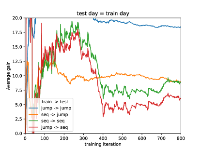
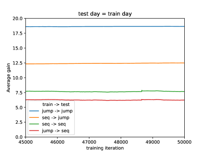
Figure 1: Average total gain of a market maker agent as a function of agent’s number of update for various combinations of train / test time evolution scheme; test on the same day as the training, after training. Left plot: zoom on the start of the testing periods; right plot: zoom over the last part of the testing periods. 48 agents were trained for each day and for each time evolution scheme; 15,000 training iterations. Data: Total Energies 2016-01-05 to 2016-01-08.

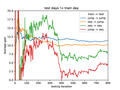
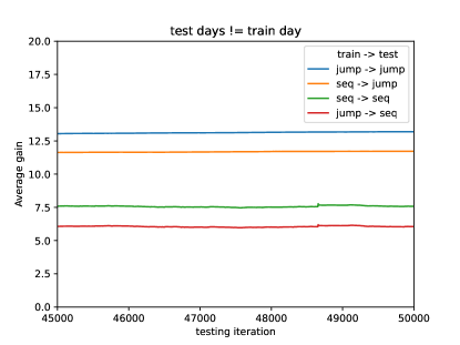
Figure 2: Average total gain of a market maker agent as a function of agent’s number of iterations for various train / test time evolution types. Left plot: zoom on the start of the testing periods; right plot: zoom over the last part of the testing periods. Cross-validation over 5 days; 48 runs per day and time evolution type; 15,000 training iterations. Data: Total Energies 2016-01-05 to 2016-01-08.

Finally, we compute the signal-to-noise ratio of the reward per update (Fig. 3), which is mechanically larger when there are more test days (right hand side plot). One first sees that using data time travel yields a better risk-adjusted reward when train in the same way, and eventually for the agents trained with sequential data. For intermediate times, the signal-to-noise ratio is essentially the same for this kind of agents when tested on either sequential data or with data time travel. However, during the first $\sim$5000 updates, the signal-to-noise ratios of their gains are the same for either time dynamics in the test phase; we interpret this as the time needed to learn how to exploit the new type of time dynamics

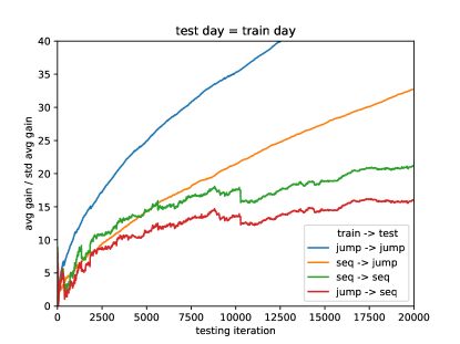
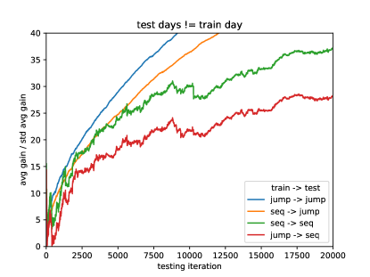
Figure 3: Signal-to-noise ratio of the gain of a market maker agent as a function of agent’s number of update for various combinations of train / test time evolution scheme; test on the same day as the training, after training. Left plot: testing on the same day as training; right plot: testing on non-training days. 48 agents were trained for each day and for each time evolution scheme; 15,000 training iterations. Data: Total Energies 2016-01-05 to 2016-01-08.

6 Discussion

Using anonymous data for offline RL in a competitive multi-agent system is possible, provided that one cares to use them in a consistent way, which naturally suggests to exploit data time travel in order to find consistent trajectories. While we used limit order books as a textbook example of such systems, the validity of our approach is not restricted to financial markets. Market making in limit order books provided indeed an ideal application of data time travel. Compared to the usual naive zero-impact sequential way, data time travel yields a better signal-to-noise ratio and a more consistent loss of gains between the test and the train periods. The importance of taking one’s impact, however small, in a competitive multi-agent competitive system was investigated in simple games, which clearly shows that it leads to qualitatively different global and individual behaviour, incidentally by also increasing the signal-to-noise ratio of agent payoffs (Marsili et al., 2000; Challet et al., 2004).

The clear difference of outcomes between agents trained and tested on either sequential data or with date time travel shows that the agents learn a different dynamics. In our opinion, using data in a more consistent way takes more consistent paths, i.e., paths closer to those that the system would have taken if the agents had been playing against it. This is probably why the gain seems to be larger for agents trained and tested on consistently jumping data. The fact that the payoff is larger when using data time travel suggests that wrong conclusions about the difficulty of training market maker with RL may be inferred, for example the difficulty of achieving positive payoffs.

We have also emphasized the importance of accounting for the facts that the actions of a RL agent do not translate into the same set of effective actions on the system, and that accounting explicitly for the influence of the different types of latency make the whole problem of consistent dynamics more intricate.

While conceptually data time travel makes better use of the available data, its level of consistency depends on how well the system dynamics is encoded by the chosen system state encoding and influence matching. For example, we neglected the dynamics of the system before the current time when looking for compatible jump times, which can be remedied in a straightforward way for example by include an encoding of the last few events in the limit order book. More generally, we chose a fairly simplified setup here which has the advantage of speed. A more realistic approach would require to use continuous variables and computing distances between dim indices, with partial and possibly expanding index sampling. This is left for future work. Finally, we plan to investigate data time travel for training a RL speculative agent acting at a high enough frequency.

References

- Abergel et al. (2016) Frédéric Abergel, Marouane Anane, Anirban Chakraborti, Aymen Jedidi, and Ioane Muni Toke. Limit order books. Cambridge University Press, 2016.
- Barzykin et al. (2023) Alexander Barzykin, Philippe Bergault, and Olivier Guéant. Algorithmic market making in dealer markets with hedging and market impact. Mathematical Finance, 33(1):41–79, 2023.
- Bergault et al. (2021) Philippe Bergault, David Evangelista, Olivier Guéant, and Douglas Vieira. Closed-form approximations in multi-asset market making. Applied Mathematical Finance, 28(2):101–142, 2021.
- Bouchaud et al. (2018) Jean-Philippe Bouchaud, Julius Bonart, Jonathan Donier, and Martin Gould. Trades, quotes and prices: financial markets under the microscope. Cambridge University Press, 2018.
- Challet et al. (2004) Damien Challet, Matteo Marsili, and Yi-Cheng Zhang. Minority games: interacting agents in financial markets. OUP Oxford, 2004.
- Chiarella (1992) Carl Chiarella. The dynamics of speculative behaviour. Annals of operations research, 37(1):101–123, 1992.
- Eisler et al. (2012) Zoltan Eisler, Jean-Philippe Bouchaud, and Julien Kockelkoren. The price impact of order book events: market orders, limit orders and cancellations. Quantitative Finance, 12(9):1395–1419, 2012.
- Frey et al. (2023) Sascha Yves Frey, Kang Li, Peer Nagy, Silvia Sapora, Christopher Lu, Stefan Zohren, Jakob Foerster, and Anisoara Calinescu. Jax-lob: A gpu-accelerated limit order book simulator to unlock large scale reinforcement learning for trading. In Proceedings of the Fourth ACM International Conference on AI in Finance, pages 583–591, 2023.
- Guéant (2017) Olivier Guéant. Optimal market making. Applied Mathematical Finance, 24(2):112–154, 2017.
- Hambly et al. (2023) Ben Hambly, Renyuan Xu, and Huining Yang. Recent advances in reinforcement learning in finance. Mathematical Finance, 33(3):437–503, 2023.
- Kumar (2020) Pankaj Kumar. Deep reinforcement learning for market making. In Proceedings of the 19th International Conference on Autonomous Agents and MultiAgent Systems, pages 1892–1894, 2020.
- Lehalle and Laruelle (2018) Charles-Albert Lehalle and Sophie Laruelle. Market microstructure in practice. World Scientific, 2018.
- Levine et al. (2020) Sergey Levine, Aviral Kumar, George Tucker, and Justin Fu. Offline reinforcement learning: Tutorial, review, and perspectives on open problems. arXiv preprint arXiv:2005.01643, 2020.
- Lillo and Farmer (2004) Fabrizio Lillo and J Doyne Farmer. The long memory of the efficient market. Studies in Nonlinear Dynamics & Econometrics, 8(3), 2004.
- Marsili et al. (2000) Matteo Marsili, Damien Challet, and Riccardo Zecchina. Exact solution of a modified el farol’s bar problem: Efficiency and the role of market impact. Physica A: Statistical Mechanics and its Applications, 280(3-4):522–553, 2000.
- Mnih et al. (2015) Volodymyr Mnih, Koray Kavukcuoglu, David Silver, Andrei A Rusu, Joel Veness, Marc G Bellemare, Alex Graves, Martin Riedmiller, Andreas K Fidjeland, Georg Ostrovski, et al. Human-level control through deep reinforcement learning. Nature, 518(7540):529–533, 2015.
- Schrittwieser et al. (2020) Julian Schrittwieser, Ioannis Antonoglou, Thomas Hubert, Karen Simonyan, Laurent Sifre, Simon Schmitt, Arthur Guez, Edward Lockhart, Demis Hassabis, Thore Graepel, et al. Mastering atari, go, chess and shogi by planning with a learned model. Nature, 588(7839):604–609, 2020.
- Spooner et al. (2018) Thomas Spooner, John Fearnley, Rahul Savani, and Andreas Koukorinis. Market making via reinforcement learning. In Proceedings of the 17th International Conference on Autonomous Agents and MultiAgent Systems, pages 434–442, 2018.
- Sutton and Barto (2018) Richard S Sutton and Andrew G Barto. Reinforcement learning: An introduction. MIT press, 2018.