Network Fission Ensembles for Low-Cost Self-Ensembles

Abstract

Recent ensemble learning methods for image classification have been shown to improve classification accuracy with low extra cost. However, they still require multiple trained models for ensemble inference, which eventually becomes a significant burden when the model size increases. In this paper, we propose a low-cost ensemble learning and inference, called Network Fission Ensembles (NFE), by converting a conventional network itself into a multi-exit structure. Starting from a given initial network, we first prune some of the weights to reduce the training burden. We then group the remaining weights into several sets and create multiple auxiliary paths using each set to construct multi-exits. We call this process Network Fission. Through this, multiple outputs can be obtained from a single network, which enables ensemble learning. Since this process simply changes the existing network structure to multi-exits without using additional networks, there is no extra computational burden for ensemble learning and inference. Moreover, by learning from multiple losses of all exits, the multi-exits improve performance via regularization, and high performance can be achieved even with increased network sparsity. With our simple yet effective method, we achieve significant improvement compared to existing ensemble methods. The code is available at https://github.com/hjdw2/NFE.

1 Introduction

Forming an ensemble of multiple neural networks is one of the easiest and most effective ways to enhance the performance of deep neural networks for image classification [8, 15, 16]. Simple combination, such as majority vote or averaging the outputs of multiple models, can significantly improve the generalization performance [2, 5]. Despite its simplicity, however, it is difficult to use such a method when the model size or the number of training data increases since it requires a significant amount of computational resources.

In order to overcome this limitation, several ensemble learning methods with low extra computational costs have recently been proposed. To reduce the training burden of ensemble learning, these methods obtain multiple trained models using efficient approaches, such as exploiting smaller pruned sub-networks instead of intact original networks [30, 22], obtaining multiple models through a single learning process using a cyclic learning rate schedule [13, 7], or training a single network structure that embeds multiple ensemble members [28, 9]. However, although the additional cost of obtaining multiple trained models is diminished, the ensemble inference process still requires computation through multiple models. Thus, if the sizes of the neural networks increase, these methods suffer from computational burdens, especially memory complexity for loading the models. Pruned sub-networks can be employed to alleviate the problem, but their performance usually decreases with increasing the sparsity (i.e., the ratio of the removed weights), making it difficult to achieve high ensemble performance.

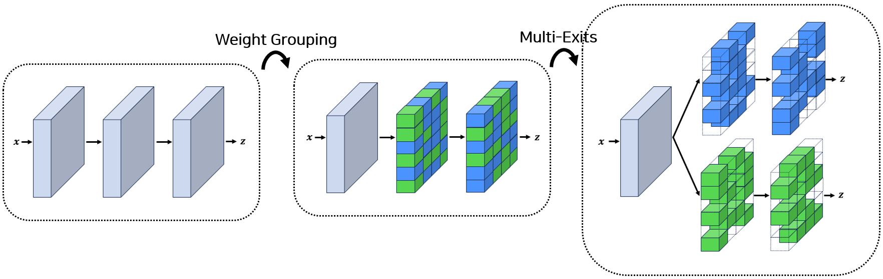
(a) Illustration of the Network Fission process

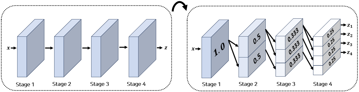
(b) Example of Network Fission with a balanced weight grouping strategy to obtain four exits. On the right side, the sparsity of layers in each stage is also shown.

Figure 1: We group the weights of layers in the stage into several sets and create multiple auxiliary classifier paths (exits) to construct multi-exits. This Network Fission enables us to obtain multiple outputs with a single network for ensemble learning at almost zero-cost.

In this paper, we propose a new ensemble learning method to obtain multiple outputs with a single conventional network (e.g., ResNet [10]) without additional modules, which is free from the above fundamental problems of ensemble learning and inference. To obtain multiple outputs constructing an ensemble, our method turns the network into a structure having multi-exits. First, weight pruning is performed on the network to reduce the training burden. Then, we group the weight parameters in each ‘stage’ (referring to the layer block repeatedly used multiple times in the network) and create multiple auxiliary paths using each of them as shown in Figure 1, which we call Network Fission. By the Network Fission process, the network becomes multi-exits with multiple auxiliary paths, which yield different outputs. After training the multi-exits, the outputs of all exits are combined for ensemble inference. Thus, ensemble inference can be performed only with one network without the need to load multiple models. We call our method Network Fission Ensembles (NFE).

Our NFE does not use additional networks for both training and inference and only changes the network structure (computation process) using the existing weights. Therefore, there is no addition in the number of parameters and memory usage, which means that it enables ensemble learning and inference at almost zero-cost. In addition, NFE can also benefit from multi-exit learning. Since the training losses of all exits are optimized together, it converges to a better optimum that can satisfy all losses via regularization. Therefore, the performance of each path itself is improved, and consequently the performance of the ensemble is also enhanced compared to the ensemble of individual networks trained separately. Thus, although the sparsity of the entire network is increased by pruning to reduce the computational burden, NFE can achieve high performance. Moreover, to simplify the pruning process, we use the pruning-at-initialization (PaI) method, which incurs an almost negligible amount of operation and requires no extra process after training begins. We show that NFE achieves highly satisfactory performance at low cost and is also effective compared to other state-of-the-art ensemble methods.

To sum up, our contributions are as follows: We propose a new low-cost ensemble learning method, NFE, by grouping weights into several sets and creating multiple paths to construct multi-exits, which enables to obtain multiple outputs for ensemble learning. We demonstrate that NFE achieves better results than previous state-of-the-art low-cost ensemble methods.

The remainder of the paper is organized as follows. Section 2 reviews the related work. In Section 3, the proposed NFE method is described in detail. Section 4 presents experimental results. Finally, conclusions are made in Section 5.

2 Related Work

2.1 Ensemble Learning

Various methods have been proposed to reduce the computational burden of ensemble learning. There are three types of research streams for low-cost ensemble learning.

The first type applies some modification to the network itself to obtain several different outputs and construct ensembles. TreeNet [21] adds several additional branches in the middle of the network, but spends significant computational and memory cost due to the increased model size. Monte Carlo Dropout [6] uses dropout [25] not only at the training phase but also at the inference phase for uncertainty estimation. BatchEnsemble [28] changes each weight matrix to the product of a shared weight and an individual rank-one matrix. Multi-Input Multi-Output Ensembles (MIMO) [9] introduces a multi-input multi-output configuration in the network. These can be memory-efficient, but the diversity among the ensemble members is limited since most parts of the network are shared among the ensemble members, which results in the limitation in the ensemble performance.

The second type uses different learning configurations to obtain differently trained models having the same structure. An example is the method of training the same network multiple times with different initialization, which is one of the simplest forms of an ensemble [3]. Snapshot Ensembles (SSE) [13] and Fast Geometric Ensembles (FGE) [7] use cyclic learning rate schedules and save multiple checkpoints that correspond to ensemble members. HyperEnsembles [29] uses different hyperparameter configurations to obtain different models. Since these methods need to use multiple models for ensemble inference, as the model size increases, they suffer from increased memory complexity for loading the models.

The third type exploits smaller pruned sub-models for ensembles. FreeTickets Ensembles [22] obtains sub-models during the training of a main dense network by pruning. Prune and Tune Ensembles (PAT) [30] obtains sub-models by pruning a trained main dense network. However, there is a trade-off between sparsity and performance in these methods. As sparsity increases to improve efficiency, the number of sub-models needed to maintain performance increases, which deteriorates the low-cost advantage.

To overcome the limitations of the existing methods, we propose a more efficient way to enable high-performance ensemble inference only with a single model.

2.2 Multi-Exits

A multi-exit structure refers to a model having one or more auxiliary classifiers (exits) in addition to the main network classifier, where parts of the network are shared among the exits. Neural networks having multi-exits have been used for different purposes, such as anytime prediction [12], performance improvement [19], structural optimization [18], etc. The multi-exit structures can be broadly categorized into two types. The first type is a specially designed network considering the multi-output structure with a specific purpose, such as anytime prediction or low computational budget [12, 24], which is less versatile. The other type attaches auxiliary classifiers to a conventional network [32, 19], which is applicable to diverse model structures. However, in the latter approach, there is no general criterion to determine the structure of exits, and it is usually designed heuristically. In [19], it is attempted to develop a criterion for constructing the exits for performance maximization. However, it is applicable to only certain kinds of networks. In our method, there is no need to determine the structures of the exits a priori, which provides a more consistent and simpler solution.

2.3 Network Pruning

Pruning is a method of compressing neural networks by removing the weight parameters that have less significance to the accuracy. There exist two approaches depending on whether pruning is performed after training begins or before training begins. However, since the former approach does not reduce the training burden, it is not suitable for low-cost ensemble learning [11]. Thus, we rely on the latter approach, i.e., the PaI method. Single-shot Network Pruning (SNIP) [20] and Gradient Signal Preservation (GraSP) [27] use the gradients of the training loss as a pruning criterion in a single-shot way. These single-shot methods have an undesirable possibility to eliminate all the weights in a particular layer, inducing layer-collapse when the sparsity is high [26]. Iterative Synaptic Flow Pruning (SynFlow) [26] alleviates this problem using iterative magnitude-based pruning. Recent work shows that simple random pruning without a pruning criterion can also achieve high performance just with a certain pre-defined layer-wise sparsity [23].

3 Proposed Method

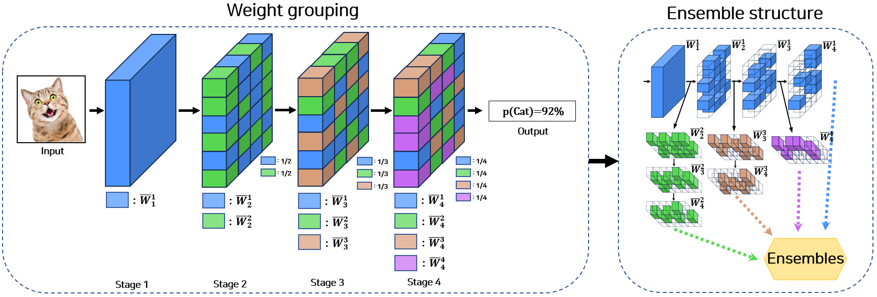
Figure 2: Illustration of the proposed Network Fission Ensembles. On the left side, weight grouping is performed considering the number of ensemble members (exits) to use ($N=4$ here). Then, the network is converted into a multi-exit structure using the grouped weights and the ensemble of the exits is obtained, as depicted on the right side. Since only the computation process is changed without any explicit structural changes, no additional training and inference burden is incurred.

3.1 Network Fission

Ensemble learning basically needs multiple outputs that can be combined for performance improvement. To achieve this, we convert a conventional network to a multi-exit structure without any additional networks. We first prune the initial network using the PaI method in order to reduce the computational burden. Then, to enable low-cost ensemble learning, we group the weights in each stage into several sets. Each set is turned into an auxiliary path (i.e., exit) that produces its own classification outputs, so a mult-exit structure is obtained as shown in Figure 2. We call this process Network Fission.

Let $W_{i}$ be the weight matrix in the $i$th stage ($i=1,...,K$) in the network and $M_{i}$ be the pruning mask for $W_{i}$ obtained by applying the PaI method to the network. $M_{i}$ is a binary matrix consisting of 0s and 1s, where each value indicates whether the weight at the corresponding location is pruned (0) or unpruned (1). Then, the remaining weights after pruning $\hbox to0.0pt{\hskip 2.91666pt\leavevmode\hbox{\set@color$\overline{\hbox{}}$}\hss}{\leavevmode\hbox{\set@color$W$}}_{i}$ is obtained by the element-wise product of $W_{i}$ and $M_{i}$.

$$\hbox to0.0pt{\hskip 2.91666pt\leavevmode\hbox{\set@color$\overline{\hbox{}}$}\hss}{\leavevmode\hbox{\set@color$W$}}_{i}=W_{i}\circ M_{i}.$$ (1)

Let $N$ be the number of ensemble members (exits) to use. For weight grouping, the weights of the last stage $\hbox to0.0pt{\hskip 2.91666pt\leavevmode\hbox{\set@color$\overline{\hbox{}}$}\hss}{\leavevmode\hbox{\set@color$W$}}_{K}$ are grouped into $N$ sets. To this end, we obtain a random number $j$ drawn from the categorical distribution ($1\leq j\leq N$) for each element for which the value of $M_{K}$ is 1. Here, the probabilities of each outcome determine the relative sizes of the exits; we observe that it is beneficial to use the same probabilities for all outcomes for balanced weight grouping to make all exits have the same size (see Section 4.1.2). Then, the grouping matrix $r^{j}_{K}$ is created, whose element is 1 if the random number is $j$ at the corresponding location and 0 otherwise. Now, the grouped weights $\hbox to0.0pt{\hskip 2.91666pt\leavevmode\hbox{\set@color$\overline{\hbox{}}$}\hss}{\leavevmode\hbox{\set@color$W$}}_{K}^{j}$ is obtained by the element-wise product of $\hbox to0.0pt{\hskip 2.91666pt\leavevmode\hbox{\set@color$\overline{\hbox{}}$}\hss}{\leavevmode\hbox{\set@color$W$}}_{K}$ and $r^{j}_{K}$.

$$\hbox to0.0pt{\hskip 2.91666pt\leavevmode\hbox{\set@color$\overline{\hbox{}}$}\hss}{\leavevmode\hbox{\set@color$W$}}_{K}^{j}=\hbox to0.0pt{\hskip 2.91666pt\leavevmode\hbox{\set@color$\overline{\hbox{}}$}\hss}{\leavevmode\hbox{\set@color$W$}}_{K}\circ r^{j}_{K}.$$ (2)

Next, the same process is performed for the weights in the penultimate stage $\hbox to0.0pt{\hskip 2.91666pt\leavevmode\hbox{\set@color$\overline{\hbox{}}$}\hss}{\leavevmode\hbox{\set@color$W$}}_{K-1}$ to obtain $N-1$ weight groups; for $\hbox to0.0pt{\hskip 2.91666pt\leavevmode\hbox{\set@color$\overline{\hbox{}}$}\hss}{\leavevmode\hbox{\set@color$W$}}_{K-2}$, $N-2$ weight groups are obtained. This process is repeated until the stage after the location at which the first exit is formed.

The reason for reducing the number of divided groups progressively by one at each stage from the last $N$th stage is to ensure that each pathway consists of a different weight composition while retaining as many weight parameters as possible. For example, if we divide only the last stage into $N$ groups while sharing all other stages among pathways, the outputs from the exits will exhibit large similarity, producing minimal ensemble impact. Conversely, if we split all stages into $N$ groups, the number of weights comprising each pathway becomes too small for each exit to have enough learning capability, which results in reduced ensemble performance. Thus, the current method is proposed to assign a sufficient number of weight parameters for each pathway and, at the same time, to maintain a certain level of diversity in outputs.

Once the grouped weights in each stage are obtained, we construct multi-exits using them. We form the exit by combining grouped weights $\hbox to0.0pt{\hskip 2.91666pt\leavevmode\hbox{\set@color$\overline{\hbox{}}$}\hss}{\leavevmode\hbox{\set@color$W$}}_{i}^{j}$ ($i=1,...,K$) having the same value of $j$. If there is no weight corresponding to the value of $j$ in the stage, the weights with $j=1$ in that stage are used. For example, when $N=4$, the input-to-output paths of the four exits are as follows (Figure 2):

• $\hbox to0.0pt{\hskip 2.91666pt\leavevmode\hbox{\set@color$\overline{\hbox{}}$}\hss}{\leavevmode\hbox{\set@color$W$}}_{1}^{1}$ $\rightarrow$ $\hbox to0.0pt{\hskip 2.91666pt\leavevmode\hbox{\set@color$\overline{\hbox{}}$}\hss}{\leavevmode\hbox{\set@color$W$}}_{2}^{1}$ $\rightarrow$ $\hbox to0.0pt{\hskip 2.91666pt\leavevmode\hbox{\set@color$\overline{\hbox{}}$}\hss}{\leavevmode\hbox{\set@color$W$}}_{3}^{1}$ $\rightarrow$ $\hbox to0.0pt{\hskip 2.91666pt\leavevmode\hbox{\set@color$\overline{\hbox{}}$}\hss}{\leavevmode\hbox{\set@color$W$}}_{4}^{1}$

• $\hbox to0.0pt{\hskip 2.91666pt\leavevmode\hbox{\set@color$\overline{\hbox{}}$}\hss}{\leavevmode\hbox{\set@color$W$}}_{1}^{1}$ $\rightarrow$ $\hbox to0.0pt{\hskip 2.91666pt\leavevmode\hbox{\set@color$\overline{\hbox{}}$}\hss}{\leavevmode\hbox{\set@color$W$}}_{2}^{2}$ $\rightarrow$ $\hbox to0.0pt{\hskip 2.91666pt\leavevmode\hbox{\set@color$\overline{\hbox{}}$}\hss}{\leavevmode\hbox{\set@color$W$}}_{3}^{2}$ $\rightarrow$ $\hbox to0.0pt{\hskip 2.91666pt\leavevmode\hbox{\set@color$\overline{\hbox{}}$}\hss}{\leavevmode\hbox{\set@color$W$}}_{4}^{2}$

• $\hbox to0.0pt{\hskip 2.91666pt\leavevmode\hbox{\set@color$\overline{\hbox{}}$}\hss}{\leavevmode\hbox{\set@color$W$}}_{1}^{1}$ $\rightarrow$ $\hbox to0.0pt{\hskip 2.91666pt\leavevmode\hbox{\set@color$\overline{\hbox{}}$}\hss}{\leavevmode\hbox{\set@color$W$}}_{2}^{1}$ $\rightarrow$ $\hbox to0.0pt{\hskip 2.91666pt\leavevmode\hbox{\set@color$\overline{\hbox{}}$}\hss}{\leavevmode\hbox{\set@color$W$}}_{3}^{3}$ $\rightarrow$ $\hbox to0.0pt{\hskip 2.91666pt\leavevmode\hbox{\set@color$\overline{\hbox{}}$}\hss}{\leavevmode\hbox{\set@color$W$}}_{4}^{3}$

• $\hbox to0.0pt{\hskip 2.91666pt\leavevmode\hbox{\set@color$\overline{\hbox{}}$}\hss}{\leavevmode\hbox{\set@color$W$}}_{1}^{1}$ $\rightarrow$ $\hbox to0.0pt{\hskip 2.91666pt\leavevmode\hbox{\set@color$\overline{\hbox{}}$}\hss}{\leavevmode\hbox{\set@color$W$}}_{2}^{1}$ $\rightarrow$ $\hbox to0.0pt{\hskip 2.91666pt\leavevmode\hbox{\set@color$\overline{\hbox{}}$}\hss}{\leavevmode\hbox{\set@color$W$}}_{3}^{1}$ $\rightarrow$ $\hbox to0.0pt{\hskip 2.91666pt\leavevmode\hbox{\set@color$\overline{\hbox{}}$}\hss}{\leavevmode\hbox{\set@color$W$}}_{4}^{4}$

Using this Network Fission process, we can obtain multiple outputs for ensemble inference using a conventional single network without any additional computational cost, and ensemble inference can be performed with a much smaller amount of computation as sparsity increases.

3.2 Training

In order to train multi-exits effectively, most of the recent works apply knowledge distillation [24, 32, 19]. Since the main network (original path) usually shows the highest performance in multi-exits, it is used as a teacher to propagate its knowledge to the other exits (students) [24, 32]. In that case, the training loss is typically given by

$$L=\sum_{n=1}^{N}CE(q_{n},y)+\alpha\sum_{n=1}^{N-1}KL(q_{n},q_{N}),$$ (3)

where $CE$ is the cross entropy, $KL$ is the Kullback-Leibler (KL) divergence, $q_{n}$ is the softmax output of the $n$th exit, $y$ is the true label, and $\alpha$ is a coefficient.

In [19], however, it is shown that combining the exits can form a powerful ensemble teacher even better than the main network teacher, called exit ensemble distillation (EED). We adopt this idea with modifications. First, the original EED employs feature distillation along with output distillation, whereas we do not use the former based on our observation that it is not essential for performance improvement. Second, the original EED considers the case where the exits inherently have different sizes (thus different performance), and therefore applies unequal contributions of the exits to the ensemble. However, since all exits have the same size in our case, we treat them equally in composing the ensemble teacher signal. Thus, the training loss in our method is written as

$$L =\sum_{n=1}^{N}\bigg{\{}CE(q_{n},y)+\alpha KL(q_{n},q_{E})\bigg{\}},$$ (4)

where $q_{E}$ is the ensemble teacher signal given by

$$q_{E} =\text{softmax}\left(\frac{z_{E}}{T}\right),$$ (5)

Here, $T$ is a temperature parameter and $z_{E}$ is obtained by

$$z_{E}=\frac{1}{N}\sum_{n=1}^{N}z_{n},$$ (6)

where $z_{n}$ is the output of the $n$th exit.

After training, we first average the outputs of all exits and then perform softmax for ensemble inference. We call our method Network Fission Ensembles (NFE).

3.3 Remarks

Since our NFE does not use any additional networks and only changes the computation process of learning and inference, there is no increase in the number of parameters or memory usage. When the computational perspective is considered, there may be a very slight increase in the amount of computation due to the use of multiple training losses instead of a single training loss, which is negligible. Therefore, NFE can be called an almost zero-cost ensemble learning method compared to other low-cost ensemble learning methods in terms of the computational burden.

4 Experiments

In this section, we thoroughly evaluate our proposed NFE. First, we perform an ablation study to confirm which configuration achieves higher accuracy with respect to the PaI method and the weight grouping strategy. Second, we evalaute the accuracy of NFE with respect to the sparsity of the whole network. Third, we evalaute the accuracy and the performance of uncertainty estimation of NFE compared to state-of-the-art low-cost ensemble learning methods. Lastly, we analyze the diversity among exits and investigate how the ensemble gain is achieved in NFE.

To this end, we evaluate the methods with ResNet and Wide-ResNet [31] for the CIFAR100 [14] and Tiny ImageNet [17] datasets. We follow the network configuration and training setting in [30]. Thus, for ResNet, we modify the configuration of the first convolution layer, including kernel size (7$\times$7 $\rightarrow$ 3$\times$3), stride (2 $\rightarrow$ 1), and padding (3 $\rightarrow$ 1), and remove the max-pooling operation. For Wide-ResNet, we do not use the dropout.

Detailed training hyperparameters are as follows. We use the stochastic gradient descent (SGD) with a momentum of 0.9 and an initial learning rate of 0.1. The batch size is set to 128 and the maximum training epoch is set to 200 for CIFAR100 and 100 for Tiny ImageNet. For CIFAR100 with ResNet, the learning rate decreases by an order of magnitude after 75, 130, and 180 epochs. For all other cases, the learning rate is decayed by a factor of 10 at half of the total number of epochs and then linearly decreases until 90% of the total number of epochs, so that the final learning rate is 0.01 of the initial value. The L2 regularization is used with a fixed constant of $5\times 10^{-4}$. $\alpha$ in Eq. (4) is set to 1. The temperature ($T$) in Eq. (5) is set to 3. For Tiny ImageNet, we initialize the network using the model pre-trained for CIFAR100. All experiments are performed using Pytorch with NVIDIA RTX 8000 graphics processing units (GPUs). We conduct all experiments three times with different random seeds and report the average results.

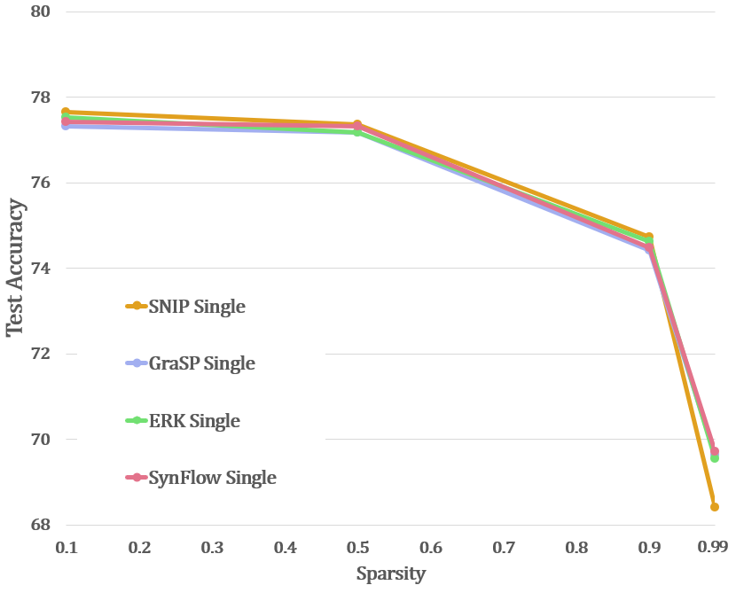
(a) Single Path

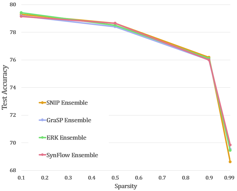
(b) Ensemble

Figure 3: Test accuracy (%) of different PaI methods with ResNet18 for CIFAR100 with respect to the sparsity.

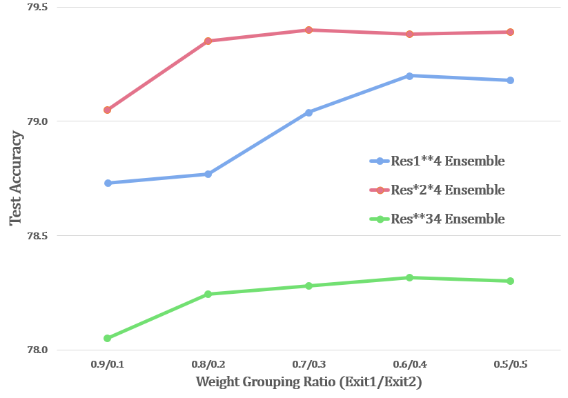
Figure 4: Test accuracy (%) for different weight grouping ratios with ResNet18 for CIFAR100.

Table 1: Comparison of the test accuracy for CIFAR100 with respect to the sparsity when ResNet18 is used as the initial network structure. The best performance at each sparsity level is marked in red.

	Accuracy (%)
Sparsity	Single	TreeNet [21] ($N$=4)	NFE ($N$=2)	NFE ($N$=4)
0	77.64	79.41	80.68	79.73
0.25	77.44	79.16	80.54	79.59
0.50	77.36	78.59	80.01	79.14
0.75	76.41	77.64	79.13	77.62

4.1 Ablation Study

We first investigate the difference in performance with respect to different types of PaI methods and weight grouping strategies. Through this, we determine which pruning method and weight grouping strategy are the best, and then set them as the learning configuration for performance comparison in the following sections. In this study, we evaluate the performance of NFE using ResNet18 trained with the cross-entropy loss for CIFAR100.

4.1.1 Pruning-at-Initialization

In order to determine which PaI method to use, we compare four PaI methods, SNIP [20], GraSP [27], Erdős-Rényi-Kernel (ERK) [23], and SynFlow [26]. As a criterion for weight pruning, SNIP and GraSP use the gradients of the training loss with respect to the weights, ERK uses a random topology with higher sparsity in larger layers, and SynFlow uses the magnitudes of the weights considering the adjacent layers’ weights. The pruning mask $M_{i}$ is generated by each method, and the performance of NFE having four exits is compared. When applying the pruning mask, we exclude the last fully-connected layer as done in [23], and also the convolution layers used for down-sampling in the residual path. These layers are highly small in size compared to the whole network, but greatly significant for performance. Thus, we do not perform pruning for these layers in all experiments.

The results are shown in Figure 3. We compare the accuracy achieved from the single main network path and the ensemble of all exits. We evaluate the four cases of sparsity: 0.1, 0.5, 0.9, and 0.99. The results show that there is no significant difference in the accuracy of both the main network and the ensemble among the PaI methods. When we extremely increase the sparsity (i.e., 0.99), differences among the methods become noticeable. However, the performance degradation is severe in all PaI methods, so this case does not have practical usage for ensemble learning. When the sparsity is below 0.99, we can get the benefit of a multi-exit ensemble. Since all the methods perform similarly in the range of sparsity (from 0.0 to 0.9) we are interested in, we choose the computationally simplest one, i.e., SNIP, as the pruning method in all of the following experiments.

4.1.2 Weight Grouping

For the Network Fission process, it is necessary to assign the proportion of weights to each exit. We compare the accuracy by varying the weight grouping ratio for each exit. To simplify the procedure, we use the multi-exits having only two exits without pruning. In this case, three kinds of network are possible, where one exit corresponds to the blue path (original main network) and the other (auxiliary exit) is one among the green, orange, and purple paths in Figure 2. We denote each network as Res1**4, Res*2*4, and Res**34, respectively.

Table 2: Comparison of the test accuracy for CIFAR100 with respect to the sparsity when Wide-ResNet28-10 is used as the initial network structure. The best performance at each sparsity level is marked in red.

	Accuracy (%)
Sparsity	Single	TreeNet [21] ($N$=3)	NFE ($N$=2)	NFE ($N$=3)
0	81.5	82.5	83.5	83.5
0.25	81.4	81.9	83.4	83.2
0.50	81.3	81.1	83.4	83.1
0.75	80.9	80.5	83.0	80.7

Figure 4 shows that the accuracy increases as the grouping ratios get more similar. When the proportions of weights in the two exits are largely unbalanced and many weights are assigned to one exit, the exit with a smaller number of weights performs poor, which contributes to the ensemble inference negligibly or even adversely. Thus, the balanced weight grouping strategy is advantageous by distributing the weights equally to all exits to prevent performance degradation of any exit and improve ensemble performance. Therefore, all following experiments use the balanced weight grouping strategy.

Table 3: Comparison of the test accuracy for Tiny ImageNet with respect to the sparsity when Wide-ResNet28-10 is used as the initial network structure. The best performance at each sparsity level is marked in red.

	Accuracy (%)
Sparsity	Single	TreeNet [21] ($N$=3)	NFE ($N$=2)	NFE ($N$=3)
0	68.2	69.0	71.0	70.6
0.25	67.9	68.5	71.0	70.2
0.50	67.4	66.9	70.9	67.7
0.75	65.0	65.3	68.4	66.6

4.2 Sparsity vs. Performance

We evaluate the performance of NFE with respect to the sparsity of the network. Although ensemble inference is an effective approach to improve performance, it is desirable to reduce the computational burden further to use it over a wide range of computational environments. Even though NFE does not introduce additional computation compared to the single network, we show that NFE can achieve high performance even when the sparsity increases.

Tables 1 and 2 show the test accuracy for CIFAR100, when ResNet18 and WRN28-10 are used as the initial network, respectively. Table 3 shows the test accuracy for Tiny ImageNet, when WRN28-10 is used as the initial network. We consider four sparsity levels (0, 0.25, 0.5, 0.75). In the tables, “Single” denotes the case when the given network structure is used without Network Fission. TreeNet [21] is included in our comparison since it is similar to our NFE in that it also performs ensemble learning by constructing multi-exits. In order to examine the effectiveness of NFE depending on the number of ensemble members (i.e., $N$), the tables present the results of NFE with the minimum and maximum numbers of members for each initial network structure. When the number of ensemble members is minimum ($N$=2), we use Res*2*4 and WRN1*3 for each network, respectively, because this setting achieves better performance.

Table 4: Performance comparison for CIFAR10 with Wide-ResNet28-10. We mark the best ensemble results in red and the second-best results in blue. The results of the methods marked with * are from [22, 30].

Method	Acc (%) $\uparrow$	NLL $\downarrow$	ECE $\downarrow$	FLOPs $\downarrow$	Epochs $\downarrow$
Single Model	96.2	0.132	0.017	3.6$\times 10^{17}$	200
Monte Carlo Dropout* [6]	95.9	0.160	0.024	1.00x	200
SSE [13] ($N$=5)*	96.3	0.131	0.015	1.00x	200
FGE [7] ($N$=12)*	96.3	0.126	0.015	1.00x	200
PAT [30] ($N$=6)*	96.5	0.113	0.005	0.85x	200
TreeNet [21] ($N$=3)	96.3	0.128	0.016	2.53x	200
BatchEnsemble [28] ($N$=4)*	96.2	0.143	0.021	4.40x	250
MIMO [9] ($N$=3)*	96.4	0.123	0.010	4.00x	250
EDST [22] ($N$=7)*	96.4	0.127	0.012	0.57x	850
DST [22] ($N$=3)*	96.4	0.124	0.011	1.01x	750
Independent Models ($N$=3)	96.5	0.122	0.016	3.00x	600
NFE ($N$=2, no pruning)	96.6	0.121	0.015	1.01x	200
NFE ($N$=2, sparsity=0.5)	96.5	0.123	0.016	0.52x	200
NFE ($N$=3, no pruning)	96.5	0.126	0.016	1.02x	200
NFE ($N$=3, sparsity=0.5)	96.3	0.137	0.017	0.53x	200

Table 5: Performance comparison for CIFAR100 with Wide-ResNet28-10. We mark the best ensemble results in red and the second-best results in blue. The results of the methods marked with * are from [22, 30].

Method	Acc (%) $\uparrow$	NLL $\downarrow$	ECE $\downarrow$	FLOPs $\downarrow$	Epochs $\downarrow$
Single Model	81.5	0.741	0.047	3.6$\times 10^{17}$	200
Monte Carlo Dropout* [6]	79.6	0.830	0.050	1.00x	200
SSE [13] ($N$=5)*	82.1	0.661	0.040	1.00x	200
FGE [7] ($N$=12)*	82.3	0.653	0.038	1.00x	200
PAT [30] ($N$=6)*	82.7	0.634	0.013	0.85x	200
TreeNet [21] ($N$=3)	82.5	0.681	0.043	2.53x	200
BatchEnsemble [28] ($N$=4)*	81.5	0.740	0.056	4.40x	250
MIMO [9] ($N$=3)*	82.0	0.690	0.022	4.00x	250
EDST [22] ($N$=7)*	82.6	0.653	0.036	0.57x	850
DST [22] ($N$=3)*	82.8	0.633	0.026	1.01x	750
Independent Models ($N$=3)	83.0	0.676	0.037	3.00x	600
NFE ($N$=2, no pruning)	83.5	0.656	0.044	1.01x	200
NFE ($N$=2, sparsity=0.5)	83.4	0.649	0.039	0.52x	200
NFE ($N$=3, no pruning)	83.5	0.658	0.061	1.02x	200
NFE ($N$=3, sparsity=0.5)	83.1	0.669	0.045	0.53x	200

In the tables, our NFE achieves significantly enhanced accuracy compared to the single model and TreeNet for both datasets. When the sparsity increases, the improvement by ensembles is maintained. Even when a half of the weights in the network are pruned, we can still obtain performance improvement by about 2% for CIFAR100 and 3% for Tiny ImageNet compared to the single model. This improvement can be attributed largely to the training loss. Although weight grouping causes partial loss of the weights in each path, distillation using the ensemble teacher can compensate for this deficiency. When the maximum possible number of ensemble members is used in NFE ($N$=3), the accuracy is slightly lowered. This is because the Network Fission process is repeated more for a larger $N$ and the number of weights in each path decreases. The performance decline is larger for a higher sparsity. Nevertheless, NFE outperforms both the single model and TreeNet in most cases.

4.3 Performance Comparison

Next, we compare the performance of NFE with other state-of-the-art low-cost ensemble learning methods, including Monte Carlo Dropout [6], SSE [13], FGE [7], PAT [30], TreeNet [21], BatchEnsemble [28], MIMO [9], and FreeTickets (Dynamic Sparse Training (DST), Efficient Dynamic Sparse Training (EDST)) [22]. We also consider the case where multiple models are independently trained and ensembled. Following [9, 22, 30], we compare the accuracy, negative log-likelihood (NLL), and expected calibration error (ECE) for CIFAR10 and CIFAR100 when the initial network structure is Wide-ResNet28-10. We also report the relative ratio of the total number of floating point operations (FLOPs) for training compared to the single model and the number of training epochs for each method.

The results for CIFAR10 and CIFAR100 are shown in Tables 4 and 5, respectively. In each table, we divide the previous methods to be compared with NFE into two categories. The methods in the first category need similar training costs to that of the single model, while the methods in the second category require much higher training costs than the first category. In order to demonstrate the performance of NFE in various cases as in the previous experiment, we show the performance of NFE when the number of ensemble members is both two and three with both the unpruned model (no pruning) and pruned model (sparsity=0.5).

Table 6: Prediction disagreement (PD) and cosine similarity (CS) between two ensemble members, and accuracy (%) of each ensemble member and the ensemble for CIFAR10 with Wide-ResNet28-10.

Method	PD	CS	Acc 1	Acc 2	Acc Ens
TreeNet [21] ($N$=2)	0.0269	0.9835	96.2	96.1	96.3
Independent Ensemble ($N$=2)	0.0274	0.9825	96.2	96.2	96.4
NFE with CE ($N$=2, no pruning)	0.0280	0.9821	96.1	96.0	96.3
NFE with CE ($N$=2, sparsity=0.5)	0.0281	0.9818	96.0	95.8	96.2
NFE with CE+KL ($N$=2, no pruning)	0.0275	0.9838	96.4	96.3	96.6
NFE with CE+KL ($N$=2, sparsity=0.5)	0.0261	0.9857	96.3	96.2	96.5

Our NFE achieves significantly enhanced accuracy compared to the other state-of-the-art low-cost ensemble methods for both datasets. Moreover, despite drastically reduced FLOPs by pruning, our method outperforms the best-performing existing methods. Even without pruning, our method shows almost no increase in FLOPs and does not require additional training epochs beyond those needed for the single model. In terms of NLL, our NFE achieves the second-best result for CIFAR10, and the difference from the best is only marginal. Similarly, for CIFAR100, our method achieves a satisfactory result with only a slight difference of 0.015 (corresponding to a relative difference of 2.37%) from the best. Although the ECE performance of our method is slightly lower compared to the best performance, our method is still comparable to most of the compared methods.

Table 7: Prediction disagreement (PD) and cosine similarity (CS) between two ensemble members, and accuracy (%) of each ensemble member and the ensemble for CIFAR100 with Wide-ResNet28-10.

Method	PD	CS	Acc 1	Acc 2	Acc Ens
TreeNet [21] ($N$=2)	0.1020	0.9470	81.3	81.2	82.4
Independent Ensemble ($N$=2)	0.1530	0.9035	81.6	81.5	82.9
NFE with CE ($N$=2, no pruning)	0.1540	0.9059	80.9	80.8	82.6
NFE with CE ($N$=2, sparsity=0.5)	0.1570	0.8983	80.8	80.5	82.5
NFE with CE+KL ($N$=2, no pruning)	0.1042	0.9410	82.8	82.7	83.5
NFE with CE+KL ($N$=2, sparsity=0.5)	0.0972	0.9491	82.7	82.6	83.4

4.4 Diversity Analysis

In general, the diversity among the ensemble members contributes to the improved classification performance of the ensemble [4, 30, 22]. To analyze the performance improvement of NFE, we evaluate the diversity of the exits in the NFE structure. As in [22, 19], we measure the pairwise diversity among ensemble members using two metrics: prediction disagreement and cosine similarity. The prediction disagreement is defined as the ratio of the number of test samples that two ensemble members classify differently [4]. The cosine similarity is measured between the softmax outputs of two ensemble members [1]. The results for $N$=2 are shown in Tables 6 and 7.

We note that the training loss directly affects the diversity in NFE. Our training loss in Eq. (4) includes the KL divergence (in addition to CE), which performs knowledge distillation for all exits using the same ensemble teacher. This would reduce the diversity among the exits compared to the case where only CE is used, which can be observed in the tables. Nevertheless, the case using both CE and KL shows higher ensemble accuracy than the case using only CE. This is because the performance of each ensemble member is greatly improved in the former case, which can be also observed in the tables. This brings an additional advantage of NFE that, even when the ensemble inference is not feasible due to certain computational constraints, it is still possible to obtain high classification accuracy using only one exit.

5 Conclusion

We proposed a new approach to ensemble learning with no additional cost, which converts the network structure into a multi-exit configuration. By grouping weights and creating auxiliary paths, our NFE constructs a multi-exit structure that learns from multiple losses, which enables effective training of the sparsified network via regularization. With the help of knowledge distillation, our method achieves improved performance by refining individual exits with the knowledge from the ensemble teacher. It was demonstrated that compared to existing low-cost ensemble learning methods, our method achieves the highest accuracy.

References

- [1] N. Dvornik, J. Mairal, and C. Schmid. Diversity with cooperation: Ensemble methods for few-shot classification. In Proceedings of the IEEE/CVF International Conference on Computer Vision (ICCV), pages 3722–3730, 2019.
- [2] S. Džeroski and B. Ženko. Is combining classifiers with stacking better than selecting the best one? Machine learning, 54:255–273, 2004.
- [3] S. Fort, H. Hu, and B. Lakshminarayanan. Deep ensembles: A loss landscape perspective. arXiv preprint arXiv:1912.02757, 2019.
- [4] S. Fort, H. Hu, and B. Lakshminarayanan. Deep ensembles: A loss landscape perspective. arXiv preprint arXiv:1912.02757, 2019.
- [5] T. M. Fragoso, W. Bertoli, and F. Louzada. Bayesian model averaging: A systematic review and conceptual classification. International Statistical Review, 86(1):1–28, 2018.
- [6] Y. Gal and Z. Ghahramani. Dropout as a bayesian approximation: Representing model uncertainty in deep learning. In Proceedings of the International Conference on Machine Learning (ICML), pages 1050–1059, 2016.
- [7] T. Garipov, P. Izmailov, D. Podoprikhin, D. P. Vetrov, and A. G. Wilson. Loss surfaces, mode connectivity, and fast ensembling of dnns. In Proceedings of the Neural Information Processing Systems (NeurIPS), volume 31, 2018.
- [8] L.K. Hansen and P. Salamon. Neural network ensembles. IEEE Transactions on Pattern Analysis and Machine Intelligence, 12(10):993–1001, 1990.
- [9] M. Havasi, R. Jenatton, S. Fort, J. Z. Liu, J. Snoek, B. Lakshminarayanan, A. M. Dai, and D. Tran. Training independent subnetworks for robust prediction. In Proceedings of the International Conference on Learning Representations (ICLR), 2021.
- [10] K. He, X. Zhang, S. Ren, and J. Sun. Deep residual learning for image recognition. In Proceedings of the IEEE/CVF Conference on Computer Vision and Pattern Recognition (CVPR), pages 770–778, 2016.
- [11] T. Hoefler, D. Alistarh, T. Ben-Nun, N. Dryden, and A. Peste. Sparsity in deep learning: Pruning and growth for efficient inference and training in neural networks. The Journal of Machine Learning Research, 22(1):10882–11005, 2021.
- [12] G. Huang, D. Chen, T. Li, F. Wu, L. v. d. Maaten, and K. Q. Weinberger. Multi-scale dense networks for resource efficient image classification. In Proceedings of the International Conference on Learning Representations (ICLR), 2018.
- [13] G. Huang, Y. Li, G. Pleiss, Z. Liu, J. E. Hopcroft, and K. Q. Weinberger. Snapshot ensembles: Train 1, get m for free. In Proceedings of the International Conference on Learning Representations (ICLR), 2017.
- [14] A. Krizhevsky. Learning multiple layers of features from tiny images. Master’s thesis, Department of Computer Science, University of Toronto, 2009.
- [15] A. Krogh and J. Vedelsby. Neural network ensembles, cross validation and active learning. In Proceedings of the Neural Information Processing Systems (NeurIPS), pages 231–238, 1994.
- [16] B. Lakshminarayanan, A. Pritzel, and C. Blundell. Simple and scalable predictive uncertainty estimation using deep ensembles. In Proceedings of the Neural Information Processing Systems (NeurIPS), volume 30, 2017.
- [17] Y. Le and X. Yang. Tiny imagenet visual recognition challenge. CS 231N, 7(7):3, 2015.
- [18] H. Lee, C.-J. Hsieh, and J.-S. Lee. Local critic training for model-parallel learning of deep neural networks. IEEE Transactions on Neural Networks and Learning Systems, 33(9):4424–4436, 2022.
- [19] H. Lee and J.-S. Lee. Rethinking online knowledge distillation with multi-exits. In Proceedings of the Asian Conference on Computer Vision (ACCV), pages 2289–2305, 2022.
- [20] N. Lee, T. Ajanthan, and P. H. S. Torr. Snip: Single-shot network pruning based on connection sensitivity. In Proceedings of the International Conference on Learning Representations (ICLR), 2019.
- [21] S. Lee, S. Purushwalkam, M. Cogswell, D. Crandall, and D. Batra. Why m heads are better than one: Training a diverse ensemble of deep networks. arXiv preprint arXiv:1511.06314, 2015.
- [22] S Liu, T Chen, Z Atashgahi, X Chen, G Sokar, E Mocanu, M Pechenizkiy, Z Wang, and D. C. Mocanu. Deep ensembling with no overhead for either training or testing: The all-round blessings of dynamic sparsity. In Proceedings of the International Conference on Learning Representations (ICLR), 2022.
- [23] S. Liu, T. Chen, X. Chen, L. Shen, D. C. Mocanu, Z. Wang, and M. Pechenizkiy. The unreasonable effectiveness of random pruning: Return of the most naive baseline for sparse training. In Proceedings of the International Conference on Learning Representations (ICLR), 2022.
- [24] M. Phuong and C. Lampert. Distillation-based training for multi-exit architectures. In Proceedings of the IEEE/CVF International Conference on Computer Vision (ICCV), pages 1355–1364, 2019.
- [25] N. Srivastava, G. Hinton, A. Krizhevsky, I. Sutskever, and R. Salakhutdinov. Dropout: A simple way to prevent neural networks from overfitting. Journal of Machine Learning Research, 15(56):1929–1958, 2014.
- [26] H. Tanaka, D. Kunin, D. L. Yamins, and S. Ganguli. Pruning neural networks without any data by iteratively conserving synaptic flow. In Proceedings of the Neural Information Processing Systems (NeurIPS), volume 33, pages 6377–6389, 2020.
- [27] C. Wang, G. Zhang, and R. Grosse. Picking winning tickets before training by preserving gradient flow. In Proceedings of the International Conference on Learning Representations (ICLR), 2020.
- [28] Y. Wen, D. Tran, and J. Ba. Batchensemble: an alternative approach to efficient ensemble and lifelong learning. In Proceedings of the International Conference on Learning Representations (ICLR), 2020.
- [29] F. Wenzel, J. Snoek, D. Tran, and R. Jenatton. Hyperparameter ensembles for robustness and uncertainty quantification. In Proceedings of the Neural Information Processing Systems (NeurIPS), volume 33, pages 6514–6527, 2020.
- [30] T. Whitaker and D. Whitley. Prune and tune ensembles: low-cost ensemble learning with sparse independent subnetworks. In Proceedings of the Association for the Advancement of Artificial Intelligence (AAAI), volume 36, pages 8638–8646, 2022.
- [31] S. Zagoruyko and N. Komodakis. Wide residual networks. In Proceedings of the British Machine Vision Conference (BMVC), 2016.
- [32] L. Zhang, J. Song, A. Gao, J. Chen, C. Bao, and K. Ma. Be your own teacher: Improve the performance of convolutional neural networks via self distillation. In Proceedings of the IEEE/CVF International Conference on Computer Vision (ICCV), pages 3712–3721, 2019.