Various Properties of Various Ultrafilters, Various Graph Width Parameters, and Various Connectivity Systems

Abstract

Filters are collections of sets that are closed under supersets and finite intersections, serving as fundamental tools in topology and set theory. An ultrafilter, a maximal filter on a set, plays a crucial role in these fields by rigorously handling limits, convergence, and compactness. A connectivity system is defined as a pair $(X,f)$, where $X$ is a finite set and $f$ is a symmetric submodular function. Understanding the duality in these parameters elucidates the relationship between different decompositions and measures of a graph’s complexity. In this paper, we delve into ultrafilters on connectivity systems, applying Tukey’s Lemma to these systems. Additionally, we explore prefilters, ultra-prefilters, and subbases within the context of connectivity systems. Furthermore, we introduce and investigate new parameters related to width, length, and depth, enhancing our understanding of these mathematical structures. We also investigate and compare various graph width parameters and their related parameters. (It also includes information similar to that found in surveys, aiming to promote future research on graph width parameters.)

1 Introduction

1.1 Filter and Graph width parameters

Filters are essential collections of sets in topology and set theory, characterized by their closure under supersets and finite intersections. They can be viewed as a way to "focus" on certain subsets of a space, much like a lens that sharpens specific details while filtering out others. An ultrafilter, being a maximal filter on a set, is particularly significant for addressing fundamental concepts such as limits, convergence, and compactness. Its unique properties render it indispensable in various fields, including non-standard analysis, model theory, social choice theory (social judgments), group theory, boolean algebra, geometry, probability theory, vector theory, semigroup theory, abstract algebra, topology, set theory, infinite combinatorics, fuzzy theory, graph theory, matroid theory, lattice theory, and first-order logic, where it provides powerful tools for both mathematical and logical applications[373, 370, 903, 481, 347, 4, 208, 418, 591, 807, 99, 177, 678, 361, 175, 364, 250].

Graph theory, a key branch of mathematics, delves into the study of networks consisting of nodes and edges, with a focus on their paths, structures, and properties [878, 237, 123]. Among the critical metrics in this field is the "graph width parameter," which measures the maximum width across all cuts or layers within a hierarchical decomposition of the graph. This metric is crucial for analyzing a graph’s complexity and structure, serving as a primary factor in transforming computationally hard graph problems into more tractable ones when the graph class is restricted to having bounded width. Various width parameters have been rigorously explored and are widely recognized in the literature [407, 716, 285, 295, 373, 23, 759, 604, 455, 525, 339, 603, 502, 362, 836, 365]. For further information, see Appendix A, “Various Width Parameters,” and Appendix C, “Comparing Various Graph Parameters (Over 70 Parameters).”

Branch-width is an important graph width parameter, defined through branch decomposition where the leaves correspond to the graph’s edges [407, 716, 105]. It is closely related to tree-width, another significant graph width parameter. Tree-width is determined by a tree decomposition, which represents the graph as a tree structure, grouping vertices into "bags," with the tree-width being the size of the largest bag minus one [759, 754]. Conversely, branch-width involves a branch decomposition where the graph is segmented into a tree-like structure, with the branch-width representing the maximum size of the minimum cut between two parts of the graph. The relationship between branch-width (bw(G)) and tree-width (tw(G)) is given by the inequalities: bw(G) $\leq$ tw(G)+1 $\leq$ $\frac{3}{2}$ $\cdot$ bw(G) for a graph $G$ with bw(G) $\geq$ 2 [105]. This relationship shows that both parameters are linked, with tree-width generally being larger, but not excessively so. Extending tree-width to the connectivity system framework leads to the concept of branch-width, highlighting their conceptual connection.

Graph width parameters offer several significant advantages in both theoretical and practical contexts:

1. Foundational Role in Theoretical Graph Theory: Graph width parameters play a critical role in the Graph Minors project serving as a fundamental combinatorial tool [407, 716]. This project, which is pivotal in the structure theory of graphs, uses graph width parameters to explore graph properties and their relationships through a series of influential theorems and algorithms.

2. Algorithmic Efficiency: Graph width parameters are conducive to algorithmic applications, particularly in the field of fixed-parameter tractable (FPT) algorithms [325, 375, 313, 798]. Algorithms that are parameterized by Graph width parameters often demonstrate superior efficiency and are widely utilized in computational graph theory. This aspect is particularly valuable in optimizing complex computations and in the development of algorithms that can efficiently solve problems considered intractable by other means.

3. Practical Applicability: In real-world applications, graphs derived from various domains such as programming language [173, 833], road networks [909, 874], and organizational structures [700] often exhibit small width. This characteristic simplifies complex problems, making them more manageable and allowing for the application of advanced graph algorithms. As a result, studying graph width parameters can directly impact the effectiveness and efficiency of practical solutions in engineering, software development, and logistics [868, 185, 891, 791, 173, 236, 545, 239].

A pair $(X,f)$, consisting of a finite set $X$ and a symmetric submodular function $f$, is recognized as a connectivity system [407]. This concept is widely utilized in the analysis of graph structures, particularly in relation to graph width parameters such as branch-width and tree-width [407, 716, 373]. Exploring the duality (the min-max theorem) within these parameters enhances our understanding of the relationships among various graph decompositions and measures of graph complexity. In this context, "duality" refers to a theorem or relationship where the presence (or absence) of one entity implies the absence (or presence) of its corresponding dual entity, often referred to as a minmax theorem [780]. Ultrafilters on connectivity systems are known to exhibit such a dual relationship with branch-width [373]. Concepts like ultrafilters, often termed as obstructions, play a crucial role in determining the values of graph width parameters.

1.2 Our Contribution

This paper outlines our contributions as follows:

• Section 2: We primarily explain the basic concepts of ultrafilters on connectivity systems and graph-width parameters, along with previously known concepts. We discuss the relationship between ultrafilters on connectivity systems and well-known concepts like Tangle from Graph Minor theory and Matroid commonly used in optimization theory.

• Section 3: We delve into ultrafilters on connectivity systems, considering Tukey’s Lemma for these systems. Tukey’s Lemma asserts that every non-empty collection of sets, closed under supersets, contains a maximal element. This fundamental result in set theory is often used to prove the existence of ultrafilters and related concepts [903, 481, 4]. Additionally, we explore chains and antichains on connectivity systems.

• Section 4: We discuss prefilters, ultra-prefilters, and subbases on connectivity systems. Prefilters, ultra-prefilters, and subbases are known concepts used to generate filters and are studied in various fields. This exploration enhances our understanding of these concepts in Set Theory and their significance in different mathematical and logical contexts.

• Section 5: We examine the connectivity system discussed for finite sets from the perspective of infinite connectivity systems and countable connectivity systems. We analyze the properties of ultrafilters on these connectivity systems.

• Section 6: We investigate new many parameters such as width, length, and depth, as well as the Ultrafilter game on connectivity systems, ultraproduct on connectivity systems, and the Axiom of Choice on connectivity systems. We also consider a Small Set Expansion [885, 48, 897, 168, 305, 89].

• Appendix: This section presents an investigation and comparison of various graph width parameters and their related parameters. It also includes information similar to that found in surveys, aiming to promote future research on graph width parameters.

We aim to make new contributions to the study of Graph Width Parameters and Graph Algorithms by interpreting key concepts like Tree-decomposition, Branch-decomposition, Tangles, and their related graph parameters through the lens of various mathematical disciplines. For instance, in this paper, we explore concepts from Set Theory (Ultrafilter, prefilter), Lattice Theory (chain, antichain), Model Theory (Ultraproduct), Hypergraph Theory (clutter), Matroid Theory (Matroid Path-width, single-element-extension), Fuzzy Theory (Fuzzy Tree-width), First-order Logic (weak ultrafilter), Social Judgment (Quasi Ultrafilter), Game Theory (cops and robbers, simple game), and Sperner Theory (Sperner system and trace), among others.

Note 1.1.

Please note that preprints and early-stage research may not have undergone peer review. Additionally, as I am an independent researcher, please understand. Sorry.

Contents

1. 1 Introduction
   1. 1.1 Filter and Graph width parameters
   2. 1.2 Our Contribution
2. 2 Definitions and Notations in this paper
   1. 2.1 Notation in this paper
      1. 2.1.1 Notation for Set theory
      2. 2.1.2 Notation for undirected graph
      3. 2.1.3 Notation for directed graph
   2. 2.2 Symmetric Submodular Function and Connectivity System
   3. 2.3 Ultrafilter on Connectivity System
      1. 2.3.1 Ultrafilter for set theory
      2. 2.3.2 Ultrafilter on Connectivity system
      3. 2.3.3 Relation between Tangle and Ultrafilter
      4. 2.3.4 Bramble and Ultrafilter
      5. 2.3.5 Other concepts related to filters on a connectivity system
   4. 2.4 Branch width on Connectivity System
      1. 2.4.1 Branch width
      2. 2.4.2 Linear Branch width
3. 3 Tukey’s Lemma and Chain for Connectivity Systems
   1. 3.1 Chain for Connectivity Systems
   2. 3.2 Tukey’s Lemma for Connectivity System
   3. 3.3 Antichain for Connectivity Systems: Relationship among Ultrafilter, Chain, and Antichain
   4. 3.4 Sequence of connectivity system
   5. 3.5 Other concepts on connectivity system
      1. 3.5.1 Separation chain on connectivity system
      2. 3.5.2 Sperner system on connectivity system
      3. 3.5.3 Chain-Decomposition on connectivity system
      4. 3.5.4 Operation and Single-element-chain on a Connectivity System
4. 4 Prefilter and Filter Subbase on a Connectivity System
   1. 4.1 Prefilter on a Connectivity System
   2. 4.2 Filter Subbase on a Connectivity System
   3. 4.3 Ultrafilter Number
5. 5 Ultrafilter on Infinite Connectivity System and Countable Connectivity System
   1. 5.1 Ultrafilter on Infinite Connectivity System
      1. 5.1.1 P-point and Q-point on an infinite connectivity system
   2. 5.2 Ultrafilter on Countable Connectivity System
   3. 5.3 Elimination Games with an Invisible Robber on a Countable Connectivity System
   4. 5.4 Ultrafilter on Maximum-Connectivity System
6. 6 Future Tasks
   1. 6.1 New Width/Length/Depth Parameters and Obstructions
      1. 6.1.1 Consideration about a Branch Distance Decomposition
      2. 6.1.2 Consideration about a Directed Tree Distance Decomposition
      3. 6.1.3 New Linear Width Parameter
      4. 6.1.4 Matroid Length Parameters
      5. 6.1.5 Branch-breadth and Linear-Breadth
      6. 6.1.6 Examination for Directed proper-path-width
      7. 6.1.7 Fuzzy Tree-width
      8. 6.1.8 Graph parameters for Fuzzy HyperGraph
      9. 6.1.9 Directed Hypertree Width
      10. 6.1.10 Weighted Width
      11. 6.1.11 Directed Linear-width
      12. 6.1.12 Directed Connectivity system
      13. 6.1.13 DAG-PathWidth and Related Parameter
   2. 6.2 Consideration about Property of an Ultrafilter
      1. 6.2.1 Simple Game on a Connectivity System
      2. 6.2.2 The Axiom of Choice in the Context of Connectivity Systems
      3. 6.2.3 Ultraproducts and Ultrapowers on Connectivity Systems
      4. 6.2.4 Algorithm of Constructing an Ultrafilter on a Connectivity System
      5. 6.2.5 Ultrafilter Width under Small Set Connectivity Expansion Hypothesis
      6. 6.2.6 Various Ultrafilters on a Connectivity System
   3. 6.3 Other research Themes for graph width parameters
7. 7 Acknowledgments
8. 8 Conflict of Interest
9. A Various Width Parameters
   1. A.1 Tree-width
      1. A.1.1 Hierarchy for treewidth
      2. A.1.2 Related concepts for tree-width
      3. A.1.3 Application aspect for tree-width
   2. A.2 Path-width
      1. A.2.1 Hierarchy for path-width
      2. A.2.2 Related concepts for path-width
      3. A.2.3 Application aspect for path-width
   3. A.3 Cut-width
      1. A.3.1 Hierarchy for cut-width
      2. A.3.2 Related concepts for cut-width
      3. A.3.3 Application aspect for cut-width
   4. A.4 MIM-width
      1. A.4.1 Hierarchy for MIM-width
      2. A.4.2 Related concepts for MIM-width
   5. A.5 Linear MIM-width
      1. A.5.1 Related concepts for Linear-MIM-width
   6. A.6 Boolean-width
   7. A.7 Linear-Boolean-width
   8. A.8 Band-width
      1. A.8.1 Hierarchy for Band-width
   9. A.9 Boundary-width
   10. A.10 Carving-width
       1. A.10.1 Related concept for Carving-width
       2. A.10.2 Application for carving-width
   11. A.11 Branch-width
       1. A.11.1 Hierarchy for branch-width
   12. A.12 Linear Branch-width
       1. A.12.1 Hierarchy for Linear-branch-width
   13. A.13 Rank-width
       1. A.13.1 Hierarchy for rank-width
       2. A.13.2 Related concept for rank-width
   14. A.14 Clique-width
       1. A.14.1 Hierarchy for clique-width
       2. A.14.2 Related concepts for clique-width
   15. A.15 Linear-Clique-width
       1. A.15.1 Hierarchy for Linear-Clique-width
   16. A.16 NLC-width
       1. A.16.1 Hierarchy for NLC-width
   17. A.17 Linear NLC-width
       1. A.17.1 Hierarchy for Linear-NLC-width
   18. A.18 Hypertree-width
       1. A.18.1 Related concepts for Hypertree-width
       2. A.18.2 Applications for Hypertree-width
   19. A.19 Modular-width
       1. A.19.1 Hierarchy for Modular-width
   20. A.20 Submodular-width
   21. A.21 Amalgam-width
   22. A.22 Kelly-width
       1. A.22.1 Hierarchy for Kelly-width
   23. A.23 Monoidal Width
   24. A.24 Tree-cut Width
       1. A.24.1 Related Concepts for tree-cut width
   25. A.25 Resolution width
   26. A.26 Twin-width
       1. A.26.1 Hierarchy for Twin-width
       2. A.26.2 Related concepts for Twin-width
   27. A.27 Decomposition width
   28. A.28 Minor-matching hypertree width
   29. A.29 Tree-clique width
   30. A.30 Tree-distance-width
       1. A.30.1 Hierarchy for Tree-distance-width
   31. A.31 Path-distance-width
       1. A.31.1 Hierarchy for Path-distance-width
   32. A.32 Tree-partition-width
       1. A.32.1 Hierarchy for Tree-partition-width
   33. A.33 Path-partition-width
       1. A.33.1 Hierarchy for Path-partition-width
   34. A.34 CV-width
   35. A.35 Dominating-set-width
   36. A.36 Point width
   37. A.37 Neighbourhood width
   38. A.38 Fusion-width
       1. A.38.1 Hierarchy for Fusion-width
   39. A.39 Directed NLC width
   40. A.40 Directed Tree-width
       1. A.40.1 Hierarchy for Directed Tree-width
   41. A.41 Directed path-width
       1. A.41.1 Hierarchy for Directed Path-width
   42. A.42 Directed Branch-width
   43. A.43 Directed Cut-width
   44. A.44 Directed Clique-width
   45. A.45 Directed Linear-NLC-width
       1. A.45.1 Hierarchy for Linear-NLC-width
   46. A.46 Directed Neighbourhood width
       1. A.46.1 Hierarchy for Neighbourhood width
   47. A.47 Directed Rank-width
   48. A.48 Directed Linear-Rank-width
       1. A.48.1 Hierarchy for Directed Linear-Rank-width
   49. A.49 Elimination width
   50. A.50 Flip-width
       1. A.50.1 Hierarchy for Flip-width
   51. A.51 Stretch-width
       1. A.51.1 Hierarchy for Stretch-width
   52. A.52 Cops-width
       1. A.52.1 Hierarchy for cops-width
       2. A.52.2 Related concepts for cops-width
   53. A.53 Perfect matching width
   54. A.54 Bisection-width
   55. A.55 Maximum matching width
       1. A.55.1 Hierarchy for Maximum matching width
   56. A.56 Linear Maximum Matching width
       1. A.56.1 Hierarchy for Linear-Maximum matching width
   57. A.57 Clustering-width
   58. A.58 Query-width
   59. A.59 Universal width
       1. A.59.1 Related concepts for Universal width
   60. A.60 Degree-width
   61. A.61 Median-width
       1. A.61.1 Related concepts for Median-width
   62. A.62 Directed Modular-width
   63. A.63 Cycle-width
   64. A.64 Arc-width
       1. A.64.1 Related concepts for arc-width
   65. A.65 Match width and braid width
   66. A.66 Clique cover width
   67. A.67 Questionable-width
   68. A.68 plane-width
   69. A.69 Scan-width
   70. A.70 v-width
   71. A.71 Cross-width
   72. A.72 Guidance-width
10. B Various Length Parameters
    1. B.1 Tree-length and Branch-length
    2. B.2 Future tasks for length parameters
11. C Comparing Various Graph Parameters (Over 70 Parameters)
12. D Various Graph Depth Parameters
    1. D.1 Tree-depth
       1. D.1.1 Hierarchy for Tree Depth
    2. D.2 Branch-depth
       1. D.2.1 Hierarchy for branch-depth
       2. D.2.2 Related Parameters for Branch-depth
    3. D.3 Rank-depth
    4. D.4 Shrub-depth
       1. D.4.1 Hierarchy for Shrub-depth
    5. D.5 Directed Tree-depth
13. E Proposal for Width-Parameters for Handling Uncertainty
    1. E.1 SuperHyperTree-width
    2. E.2 Neutrosophictree-width
    3. E.3 Rough Tree-width from an Information System

2 Definitions and Notations in this paper

This section provides mathematical definitions for each concept. Before delving into specific definitions, let’s outline the basic mathematical concepts used in this text.

2.1 Notation in this paper

We explain the notation used in this paper.

2.1.1 Notation for Set theory

In set theory, a set is a collection of distinct elements or objects, considered as an entity and often denoted with curly braces. A subset is a set where all elements are also contained within another set. Boolean algebra $(X,\cup,\cap)$ is a mathematical structure with a set $X$, union $(\cup)$, and intersection $(\cap)$, satisfying specific axioms for operations. In this paper, we consider finite sets (except in Section 5).

Note 2.1.

In this paper, we use expressions like $A\subseteq X$ to indicate that $A$ is a subset of $X$, $A\cup B$ to represent the union of two subsets $A$ and $B$ (both of which are subsets of $X$), and $A=\emptyset$ to signify an empty set. Specifically, $A\cap B$ denotes the intersection of subsets $A$ and $B$. Similarly, $A\setminus B$ represents the difference between subsets $A$ and $B$.

Definition 2.2.

The powerset of a set $A$, denoted as $2^{A}$, is the set of all possible subsets of $A$, including the empty set and $A$ itself.

Definition 2.3.

In set theory, a partition of a set is a way of dividing the set into non-overlapping, non-empty subsets, such that every element of the original set is included in exactly one subset. These subsets are called the "blocks" or "parts" of the partition (cf.[696]).

Definition 2.4.

In set theory, a separation of a set $X$ is a partition of $X$ into two disjoint, non-empty subsets $A$ and $B$ such that their union equals $X$ (i.e., $A\cup B=X$ and $A\cap B=\emptyset$). The subsets $A$ and $B$ are often referred to as the separated components of $X$.

Definition 2.5.

In set theory, the cardinality of a set refers to the number of elements in the set. For finite sets, the cardinality is simply the count of elements in the set.

Formally, the cardinality of a set $A$ is denoted by $|A|$. If there exists a bijection (a one-to-one correspondence) between two sets $A$ and $B$, they are said to have the same cardinality, i.e., $|A|=|B|$.

For more detailed information on set theory, please refer to surveys and lecture notes (ex.[617, 851, 331, 601]).

2.1.2 Notation for undirected graph

Except appendix and section 6, we consider a simple undirected graph $G$, where the vertex set is denoted by $V(G)$ and the edge set by $E(G)$. For simplicity, we will often write $G=(V,E)$, with $V$ representing the vertices and $E$ the edges. If $X$ is a subset of the vertices $V(G)$ (or the edges $E(G)$), then $X^{c}$ represents the complement set $V(G)\setminus X$ (or $E(G)\setminus X$, respectively), which includes all elements not in $X$.

Definition 2.6.

The degree of a vertex refers to the number of edges connected to it. For example, if a vertex has three edges connected to it, its degree is three.

Definition 2.7.

A path graph is a type of tree that consists of a sequence of vertices where each vertex is connected to exactly two others, except for the two endpoints, which are connected to only one other vertex. A linear ordering of a graph’s vertices is an arrangement of the vertices in a linear sequence in such a way that each vertex comes before all vertices to which it is connected by edges in the sequence, except possibly the previous vertex.

Example 2.8.

Consider the path graph $P_{4}$ consisting of four vertices $v_{1},v_{2},v_{3},v_{4}$ and three edges $\{v_{1},v_{2}\},\{v_{2},v_{3}\},\{v_{3},v_{4}\}$. The vertices can be arranged linearly as $v_{1},v_{2},v_{3},v_{4}$, which respects the edge connections, making it a valid path graph. The endpoints $v_{1}$ and $v_{4}$ are connected to only one other vertex, while the intermediate vertices $v_{2}$ and $v_{3}$ are each connected to two vertices.

Definition 2.9.

A tree is a connected, acyclic graph where any two vertices are connected by exactly one path, symbolizing hierarchical relationships. The root of a tree is the topmost node from which all other nodes descend. In a tree, vertices with a degree of 1 are called leaves, while all other vertices are referred to as inner vertices. A ternary tree is a specific type of tree where all inner vertices have a degree of 3.

Example 2.10.

Consider a tree with 7 vertices, labeled $v_{1}$ to $v_{7}$, where $v_{1}$ is the root. The edges of the tree are $\{v_{1},v_{2}\}$, $\{v_{1},v_{3}\}$, $\{v_{1},v_{4}\}$, $\{v_{2},v_{5}\}$, $\{v_{2},v_{6}\}$, and $\{v_{3},v_{7}\}$. This forms a ternary tree, as the root $v_{1}$ has three children $v_{2}$, $v_{3}$, and $v_{4}$, making it an inner vertex with degree 3. The vertices $v_{5}$, $v_{6}$, $v_{7}$, and $v_{4}$ are leaves with a degree of 1.

Definition 2.11.

A subgraph is a graph formed from a subset of a graph’s vertices and edges. A subpath is a continuous segment of a path, consisting of consecutive edges and vertices from the original path, and is useful for analyzing specific portions of larger paths.

Example 2.12.

Consider the original graph $G$ with vertices $V(G)=\{v_{1},v_{2},v_{3},v_{4},v_{5}\}$ and edges $E(G)=\{\{v_{1},v_{2}\},\{v_{2},v_{3}\},\{v_{3},v_{4}\},\{v_{4},v_{5}\}\}$. A subgraph $H$ can be formed by selecting the subset of vertices $V(H)=\{v_{2},v_{3},v_{4}\}$ and the corresponding edges $E(H)=\{\{v_{2},v_{3}\},\{v_{3},v_{4}\}\}$. This subgraph $H$ represents a subpath of the original path in $G$, highlighting a specific segment of the larger path.

Definition 2.13.

The distance between two vertices $u$ and $v$ in a graph $G=(V,E)$ is defined as the length of the shortest path connecting $u$ and $v$ in $G$. Formally, the distance $d_{G}(u,v)$ is given by:

$d_{G}(u,v)=\min\{\ell(P)\mid P\text{ is a path in }G\text{ connecting }u\text{ and }v\}$

where $\ell(P)$ denotes the length of the path $P$, which is the number of edges in $P$.

Example 2.14.

Consider the graph $G$ with vertices $V(G)=\{v_{1},v_{2},v_{3},v_{4},v_{5}\}$ and edges $E(G)=\{\{v_{1},v_{2}\},\{v_{2},v_{3}\},\{v_{3},v_{4}\},\{v_{4},v_{5}\},\{v_{1},v_{3}\}\}$.

To find the distance $d_{G}(v_{1},v_{4})$, observe that there are two paths connecting $v_{1}$ and $v_{4}$:

• Path 1: $v_{1}\to v_{2}\to v_{3}\to v_{4}$, with a length of 3 edges.

• Path 2: $v_{1}\to v_{3}\to v_{4}$, with a length of 2 edges.

The shortest path is Path 2, so the distance $d_{G}(v_{1},v_{4})$ is 2.

For more detailed information on graphs, please refer to surveys and lecture notes (ex.[747, 122, 238, 858, 121]).

2.1.3 Notation for directed graph

We define a directed graph $D$, where the vertex set is denoted by $V(D)$ and the edge set by $E(D)$. For clarity, we will use the notation $D=(V,E)$, where $V$ represents the vertices and $E$ represents the directed edges. If $X$ is a subset of either the vertex set $V(D)$ or the edge set $E(D)$, then $X^{c}$ denotes the complement, $V(D)\setminus X$ or $E(D)\setminus X$, respectively, consisting of all elements not contained in $X$.

Definition 2.15.

The degree of a vertex in a directed graph is defined by the number of directed edges incident to it, separated into in-degree and out-degree. For example, a vertex with three incoming edges has an in-degree of three.

Definition 2.16.

A path in a directed graph is a sequence of vertices where each vertex is connected to the next by a directed edge. A linear ordering of the vertices of a directed graph arranges them in a sequence such that, for each directed edge, the source vertex precedes the target vertex in the sequence.

Definition 2.17.

A tree in the context of directed graphs is a directed acyclic graph (DAG) that is connected and contains no directed cycles. A directed tree with $n$ vertices always has $n-1$ directed edges. A leaf in a directed tree is a vertex with exactly one incoming or outgoing edge, making it a terminal vertex. In this context, a node is any vertex, which can be either a leaf or an internal vertex depending on its degree. A subcubic directed tree is one in which every vertex has a total degree (in-degree plus out-degree) of at most three, meaning no vertex is connected by more than three directed edges.

For more detailed information on directed graphs, please refer to surveys and lecture notes (ex.[53, 52]).

2.2 Symmetric Submodular Function and Connectivity System

The definition of a symmetric submodular function is presented below. This concept is extensively used and discussed in numerous scholarly articles [595, 506, 51]. While symmetric submodular functions are generally defined over real numbers, this paper specifically considers those restricted to natural numbers. This submodular function is also sometimes referred to as the connectivity function [407]. Additionally, a variant of submodular function known as the submodular partition function is also well-known [29, 921]. Also, $k$-Submodular [496, 872, 871], two-dimensional submodular [663], monotone-submodular [304], and maximum-submodular [319] are also known.

Definition 2.18.

Let $X$ be a finite set. A function $f:2^{X}\rightarrow\mathbb{N}$ is called symmetric submodular if it satisfies the following conditions:

• $\forall A\subseteq X,\ f(A)=f(X\setminus A)$.

• $\forall A,B\subseteq X,\ f(A)+f(B)\geq f(A\cap B)+f(A\cup B)$.

In this paper, a pair $(X,f)$ of a finite set $X$ and a symmetric submodular function $f$ is called a connectivity system. This concept is frequently used in discussions of graph width parameters, such as branch-width and tree-width, to analyze graph structures (e.g., [244, 358, 354, 407]).

The following is an example illustrating the concept of a symmetric submodular function.

Example 2.19.

Consider a simple undirected graph $G=(V,E)$ where $V$ is the set of vertices and $E$ is the set of edges. Let $V=\{1,2,3,4\}$ and the edges $E=\{(1,2),(2,3),(3,4),(4,1)\}$, forming a cycle. Define a function $f:2^{V}\rightarrow\mathbb{N}$ as follows:

$$f(A)=|E(A,V\setminus A)|$$

where $E(A,V\setminus A)$ is the set of edges with one endpoint in $A$ and the other endpoint in $V\setminus A$. The symmetric submodularity condition is satisfied.

Example 2.20.

For a set of random variables $X_{1},X_{2},\dots,X_{n}$, the entropy function $H(S)$ for a subset $S\subseteq\{X_{1},X_{2},\dots,X_{n}\}$ is defined as the joint entropy of the variables in $S$. This function is known to be submodular and symmetric. Generally, the entropy function $H(S)$ itself is not symmetric, as it depends on the specific set of variables $S$. However, the mutual information between sets of variables, which is related to entropy, is symmetric. And note that entropy, in information theory, measures the uncertainty or randomness of a random variable’s outcomes. It quantifies the average amount of information produced by a stochastic source of data (cf.[793, 430]).

Example 2.21.

In the context of network flow, the cut-value function $f(S)$ for a subset $S\subseteq V$ (where $V$ is the set of vertices) is the total capacity of edges crossing from $S$ to $V\setminus S$. This is an example of a symmetric submodular function.

Example 2.22.

Let $\Omega=\{v_{1},v_{2},\dots,v_{n}\}$ be the set of vertices of a directed graph. For any set of vertices $S\subseteq\Omega$, define the function $f(S)$ to denote the number of edges $e=(u,v)$ such that $u\in S$ and $v\in\Omega\setminus S$. This function counts the number of edges leaving the set $S$.

The function $f(S)$ is submodular, meaning that for any two sets $A$ and $B$ with $A\subseteq B\subseteq\Omega$ and any vertex $x\in\Omega\setminus B$, it holds that:

$$f(A\cup\{x\})-f(A)\geq f(B\cup\{x\})-f(B).$$

However, $f(S)$ is not symmetric. Specifically, $f(S)$ depends on the direction of the edges, so in general, $f(S)\neq f(\Omega\setminus S)$. This asymmetry arises because the number of edges leaving $S$ is typically different from the number of edges entering $S$.

Moreover, this function can be generalized by assigning non-negative weights to the directed edges. In this case, $f(S)$ would represent the total weight of the edges leaving the set $S$, which still maintains the submodular property without being symmetric.

It is known that a symmetric submodular function $f$ satisfies the following useful properties:

Lemma 2.23.

[407] Let $X$ be a finite set. A symmetric submodular function $f$ satisfies:

1. $\forall A\subseteq X,\ f(A)\geq f(\emptyset)=f(X)=0$.

2. $\forall A,B\subseteq X,\ f(A)+f(B)\geq f(A\setminus B)+f(B\setminus A)$.

Proof 2.24.

The following results can be obtained:

1. $f(A)+f(A)=f(A)+f(A)\geq f(A\cup A)+f(A\cap A)=f(X)+f(\emptyset)=f(\emptyset)+f(\emptyset)$.

2. $f(A)+f(B)=f(A)+f(B)\geq f(A\cup B)+f(A\cap B)=f(B\setminus A)+f(A\setminus B)$.

Thus, the proof is completed.

2.3 Ultrafilter on Connectivity System

In this subsection. we consider about ultrafilter on Connectivity System. First, we consider about ultrafilter for set theory.

2.3.1 Ultrafilter for set theory

First, let’s introduce the general concept of an Ultrafilter in set theory. The definition of an Ultrafilter in Set Theory is described as follows.

Definition 2.25.

Let $X$ be a set. A collection $\mathcal{F}\subseteq 2^{X}$ is called a filter on $X$ if it satisfies the following conditions:

1. If $A$ and $B$ are both in $\mathcal{F}$, then their intersection $A\cap B$ is also in $\mathcal{F}$.

2. If $A$ is in $\mathcal{F}$ and $A\subseteq B\subseteq X$, then $B$ is also in $\mathcal{F}$.

3. The empty set $\emptyset$ is not in $\mathcal{F}$.

Definition 2.26.

A maximal filter, which cannot be extended any further while still being a filter, is called an ultrafilter. An ultrafilter satisfies an additional condition:

1. For any subset $A\subseteq X$, either $A$ is in $\mathcal{F}$ or its complement $X\setminus A$ is in $\mathcal{F}$, but not both.

Example 2.27.

Consider the set $X=\{1,2,3\}$. The collection $\mathcal{F}=\{\{1,2,3\},\{1,2\},\{2,3\},\{2\}\}$ is a filter on $X$. It satisfies all the conditions of a filter:

• The intersection of any two sets in $\mathcal{F}$ is also in $\mathcal{F}$.

• If $A$ is in $\mathcal{F}$ and $A\subseteq B\subseteq X$, then $B$ is also in $\mathcal{F}$.

• The empty set is not in $\mathcal{F}$.

Example 2.28.

Example of a filter is the Fréchet filter on an infinite set $X$. The Fréchet filter consists of all cofinite subsets of $X$ (i.e., subsets whose complements are finite). This collection forms a filter because:

• The intersection of two cofinite sets is also cofinite.

• Any superset of a cofinite set is cofinite.

• The empty set is not cofinite, so it is not in the filter.

Example 2.29.

Consider the set $X=\mathbb{R}$, the set of all real numbers. The collection $\mathcal{F}=\{A\subseteq\mathbb{R}\mid\exists M\in\mathbb{R},\ A\supseteq[M,\infty)\}$ is a filter on $\mathbb{R}$. This collection forms a filter because:

• The intersection of any two sets that contain some $[M,\infty)$ also contains a set of the form $[M^{\prime},\infty)$ for some $M^{\prime}\geq\max\{M_{1},M_{2}\}$, so it is in $\mathcal{F}$.

• If $A\in\mathcal{F}$ and $A\subseteq B\subseteq\mathbb{R}$, then $B\in\mathcal{F}$.

• The empty set does not contain any interval of the form $[M,\infty)$, so it is not in the filter.

Example 2.30.

Consider a topological space $(X,\tau)$. The collection of all dense open sets in $X$ forms a filter. This is because the intersection of two dense open sets is also a dense open set, and any superset of a dense open set is dense and open. The empty set is not dense, so it is not in the filter.

Example 2.31.

In a measure space $(X,\mathcal{M},\mu)$, where $\mu$ is a measure on the sigma-algebra $\mathcal{M}$, the collection of all subsets of $X$ that have positive measure (i.e., $\mu(A)>0$) forms a filter. This filter includes all sets with non-zero measure, and satisfies the filter conditions.

Example 2.32 (Voting system).

Consider a set $X$ that represents a collection of voters $X=\{v_{1},v_{2},\dots,v_{n}\}$. Each voter has a preference for a particular candidate in an election. We define a collection $\mathcal{F}$ of subsets of $X$ as follows (cf.[439, 49, 204, 643]):

• A subset $A\subseteq X$ belongs to $\mathcal{F}$ if the majority of voters in $A$ support a particular candidate, say Candidate $C$.

This collection $\mathcal{F}$ satisfies the properties of an ultrafilter:

1. Non-emptiness and Completeness: The set $\mathcal{F}$ is non-empty because there exists at least one subset of voters (e.g., the entire set $X$) that supports Candidate $C$.

2. Closure under Intersection: If two subsets $A$ and $B$ are in $\mathcal{F}$, meaning that the majority in both $A$ and $B$ supports Candidate $C$, then their intersection $A\cap B$ also belongs to $\mathcal{F}$ because the majority in $A\cap B$ still supports Candidate $C$.

3. Closure under Supersets: If $A$ is in $\mathcal{F}$ and $A\subseteq B\subseteq X$, then $B$ is also in $\mathcal{F}$. This is because if the majority of $A$ supports Candidate $C$, and $B$ includes all of $A$, then the majority in $B$ still supports $C$.

4. Decisiveness: For any subset $A\subseteq X$, either $A$ or its complement $X\setminus A$ is in $\mathcal{F}$. This corresponds to the idea that, in any group of voters, either the majority supports $C$ or the majority does not, with no undecided or neutral outcomes.

This voting system example illustrates an ultrafilter by capturing the idea of a decisive majority in a set of voters. In this context, the ultrafilter $\mathcal{F}$ helps identify the subsets of voters that consistently support a particular candidate across various possible groupings.

Several related concepts to Filters and Ultrafilters have been proposed. Here, we introduce just one: the Weak Filter. This concept, discussed in the field of logic, is used to interpret defaults through a generalized "most" quantifier in first-order logic [592, 774, 43, 593, 174]. The definition and an example are provided below.

Definition 2.33.

[592] Let $A,B$ be a set. A weak filter over a non-empty set $X$ is a collection $\mathcal{F}_{w}\subseteq 2^{X}$ that satisfies the following conditions:

1. If $A\in\mathcal{F}_{w}$ and $A\subseteq B\subseteq X$, then $B\in\mathcal{F}_{w}$.

2. If $A,B\in\mathcal{F}_{w}$, then $A\cap B\neq\emptyset$.

3. $X\in\mathcal{F}_{w}$.

Definition 2.34.

[592] Let $A,B$ be a set. A weak ultrafilter over a non-empty set $X$ is a complete weak filter, meaning it additionally satisfies the following condition:

1. For every $A\subseteq X$, $A\notin\mathcal{F}_{w}$ if and only if $X\setminus A\in\mathcal{F}_{w}$.

Example 2.35.

Let $I=\{1,2,3\}$. Consider the collection $\mathcal{F}_{w}=\{\{1,2,3\},\{1,2\},\{2,3\},\{1,3\}\}$. This collection $\mathcal{F}_{w}$ is a weak filter over $X$ because it satisfies the following:

• For any $A\in\mathcal{F}_{w}$ and any $A\subseteq B\subseteq X$, we have $B\in\mathcal{F}_{w}$.

• The intersection of any two sets in $\mathcal{F}_{w}$ is non-empty.

• The entire set $X=\{1,2,3\}$ is in $\mathcal{F}_{w}$.

For more detailed information for ultrafilter, please refer to surveys and lecture notes (ex.[418, 807]).

2.3.2 Ultrafilter on Connectivity system

We introduce some properties of the ultrafilter on the connectivity system $(X,f)$ as an extension of the Ultrafilter on Boolean Algebras. First, we introduce definitions of a filter and an ultrafilter on a connectivity system [373]. These concepts extend the traditional notions of filter and ultrafilter from set theory by incorporating the condition of symmetric submodularity. Also, an ultrafilter on the connectivity system $(X,f)$ is co-Maximal ideal [896] on the connectivity system $(X,f)$.

Definition 2.36 ([373]).

Let $X$ be a finite set and $f$ be a symmetric submodular function. In a connectivity system, the set family $F\subseteq 2^{X}$ is called a filter of order $k+1$ if the following axioms hold true:

• $\forall A\in F,\ f(A)\leq k$

• $A\in F,\ B\in F,\ f(A\cap B)\leq k\Rightarrow A\cap B\in F$

• $A\in F,\ A\subseteq B\subseteq X,\ f(B)\leq k\Rightarrow B\in F$

• $\emptyset\notin F$

An Ultrafilter on a connectivity system is a filter on a connectivity system that satisfies the following condition $(Q4)$. The Ultrafilter on a Connectivity System has a dual relationship with branch-width, a graph width parameter [373]. Note that an ultrafilter on a connectivity system is a non-empty and proper (i.e., $\emptyset\notin F$) family.

• $\forall A\subseteq X,\ f(A)\leq k\Rightarrow\text{either }A\in F\text{ or }X\setminus A\in F$

Definition 2.37.

[373] A filter is principal if the filter satisfies the following axiom $(QP5)$ [373]:

• $A\in F$ for all $A\subseteq X$ with $|A|=1$ and $f(A)\leq k$.

A filter is non-principal if the filter satisfies the following axiom $(Q5)$ [373]:

• $A\notin F$ for all $A\subseteq X$ with $|A|=1$.

Non-principal refers to a filter or ideal that does not contain any singletons (i.e., sets with exactly one element). It is not generated by any finite set.

If a filter is weak [351, 591, 44], the following axiom $(QW1^{\prime})$ holds instead of axiom $(Q1)$. Note that weak filter aims at interpreting defaults via a generalized ‘most’ quantifier in first-order logic [591, 44, 775, 336]. A weak filter on a connectivity system is co-Weak Ideal on a connectivity system:

• $A\in F,\ B\in F,\ f(A\cap B)\leq k\Rightarrow A\cap B\neq\emptyset$

If a filter is quasi [359, 176], the following axiom $(QQ1^{\prime})$ holds instead of axiom $(Q1)$. Note that a quasi-Ultrafilter is used to do an axiomatic analysis of incomplete social judgments [176]:

• $A\subseteq X,\ B\subseteq X,\ A\notin F,\ B\notin F\Rightarrow A\cup B\notin F$

If a filter is single [354], the following axiom $(\text{QS1})$ holds instead of axiom $(\text{Q1})$:

• For any $A\in F$, $e\in X$, if $f(\{e\})\leq k$ and $f(A\cap(X\setminus\{e\}))\leq k$, then $A\cap(X\setminus\{e\})\in F$.

In fact, by replacing the axiom $(\text{QS1})$ with the following $(\text{QSD1})$ [354]. This axiom aligns perfectly with the concept of single-element deletion [36, 887, 886] (co-operation of single-element extension [214, 37, 796, 816, 691], near to single-vertex-deletion and single-element-deletion (cf. [628, 899, 655])):

• For $A\in F$, $e\in X$, if $f(A\setminus\{e\})\leq k$, then $A\setminus\{e\}\in F$.

If a filter on a connectivity system is connected, the following holds true [355].

• For any $A,A^{\prime}\in\mathcal{F}$ with $A\cup A^{\prime}\neq X$, also $A\cap A^{\prime}$ is an element of $\mathcal{F}$.

• $\{s\}\notin\mathcal{F}$ for any $s\in X$ such that $f(\{s\})\leq k$ and $\emptyset\notin\mathcal{F}$.

Note that an equivalent form of a given ultrafilter $U\subseteq 2^{X}$ on a connectivity system is manifested as a two-valued morphism. This relationship is defined through a function $m$ where $m(A)=1$ if $A$ is an element of $U$, and $m(A)=0$ otherwise. Additionally, the function $m$ holds the value 1 for subsets where the value of the submodular function is at most $k$. This suggests that ultrafilters are well-suited for use in two-player games [42, 771], such as Cops and Robbers. Indeed, in literature [373], an ultrafilter on a connectivity system is employed as a winning strategy.

2.3.3 Relation between Tangle and Ultrafilter

A concept closely related to ultrafilters on a connectivity system is the tangle. Tangles are known to be dual to the concepts of tree-decomposition and branch-decomposition, and they are extensively used in the study of graph width parameters [407, 716, 759, 373, 760]. Tangles have played a significant role in algorithms across various fields, including graph minors, width parameters, and graph isomorphism problems. The definition of a tangle in a graph is provided below [760].

Definition 2.38.

[760] A tangle in a graph $G$ of order $k$ is a set $T$ of separations of $G$, each of order less than $k$, such that:

1. For every separation $(A,B)$ of $G$ of order less than $k$, one of $(A,B)$ or $(B,A)$ is an element of $T$.

2. If $(A_{1},B_{1}),(A_{2},B_{2}),(A_{3},B_{3})\in T$, then $A_{1}\cup A_{2}\cup A_{3}\neq G$.

3. If $(A,B)\in T$, then $V(A)\neq V(G)$.

Several related concepts to tangles have been proposed, including Directed Tangle (obstruction of Directeded Tree-width) [414], Hypertangle[13], Connected Tangle (obstruction of Connected Tree-width) [345], Distance-Tangle (obstruction of tree-distance-width) [342], Edge-Tangle[624], Matching Tangle[326], and Linear Tangle (Obstruction of Linear-width)[371].

Subsequently, the concept of a tangle in graphs was extended to matroids and connectivity systems[407]. The definition of a tangle on a connectivity system is provided below.

Definition 2.39 ([407]).

Let $X$ be a finite set and $f$ be a symmetric submodular function. A family $T\subseteq 2^{X}$ is a tangle of order $k+1$ on a connectivity system $(X,f)$ if $T$ satisfies the following axioms:

• $\forall A\in T,\ f(A)\leq k$,

• $A\subseteq X,\ f(A)\leq k\Rightarrow\text{either }(A\in T)\text{ or }(X\setminus A\in T)$,

• $A,B,C\in T\Rightarrow A\cup B\cup C\neq X$,

• $\forall e\in X,\ X\setminus\{e\}\notin T$.

A tangle of order $k+1$ is also a tangle of order $k$. Moreover, if $k$ is too large, a tangle cannot exist. The maximum $k$ for which a tangle can exist is called the tangle number, which coincides with the branch-width. The same principle applies to ultrafilters. (cf.[360, 407]) Actually, in an ultrafilter on a connectivity system, the following properties hold.

Theorem 2.40.

Let $(X,f)$ be a connectivity system. An ultrafilter of order $k+1$ on a connectivity system $(X,f)$ is also an ultrafilter of order $k$ on a connectivity system $(X,f)$.

Proof 2.41.

An ultrafilter of order $k+1$ on a connectivity system $(X,f)$ obviously holds axioms of an ultrafilter of order $k$ on a connectivity system $(X,f)$.

Given a set $Y\subseteq X$, the collection $\{A\subseteq X\mid A\subseteq Y,f(A)\leq k\}$ forms a tangle. This tangle is referred to as a principal tangle generated by the set $Y$ [435]. The set $Y$ is called the generator of this tangle [241].

A family $F$ on a connectivity system $(X,f)$ is a co-tangle if there is a tangle $T$ such that $A\in F$ if and only if $X\setminus A\in T$. Filter on a connectivity system is a co-tangle on the connectivity system. A filter on a connectivity system also satisfies the following conditions [373]:

• $A,B,C\in F\Rightarrow A\cap B\cap C\neq\emptyset$.

A Single-Filter on a connectivity system is a co-linear tangle on that system. It is important to note that a linear tangle is a concept dual to linear-width, which will be discussed later. The main difference between a linear tangle and a co-linear tangle lies in one of the sets in axiom (T2), which is replaced by a singleton set $\{e\}$. A linear tangle of order $k+1$ is also a linear tangle of order $k$. Furthermore, if $k$ is too large, a linear tangle cannot exist. In this paper, the largest possible $k$ for which a linear tangle can exist is referred to as the linear tangle number.

Single-Filter on a connectivity system also satisfies the following conditions [354]:

• $A,B\in F,\ e\in X,\ f(\{e\})\leq k\Rightarrow A\cap B\cap(X\setminus\{e\})\neq\emptyset$.

If single-filter is restricted [346], the following axiom $(\text{FLTR1})$ holds instead of axiom $(\text{FLT1})$:

• $A,B\in F,\ |A|\neq|B|,\ e\in X,\ f(\{e\})\leq k\Rightarrow A\cap B\cap(X\setminus\{e\})\neq\emptyset$.

Additionally, concepts such as Directed Ultrafilter [367] , defined on directed graphs, Edge-Ultrafilter [356], and Ultrafilter Tangle [603, 602, 605, 286], on the Abstract separation system, which abstracts the Connectivity system, have also been studied. It is fascinating to see the connection between seemingly unrelated concepts of Ultrafilter and Tangle when the condition of symmetric submodularity is applied.

2.3.4 Bramble and Ultrafilter

It is known that a Bramble can be constructed using a concept essentially equivalent to an Ultrafilter on separation [244]. A Bramble (cf. Strict Bramble[611]) is recognized in graph game theory, particularly in the Cops and Robbers game, as an obstruction to well-known graph width parameters such as escape routes and tree-width [474].

For reference, the definition of a bramble in a graph is introduced below[779, 114].

Definition 2.42.

[779, 114] Let $G=(V,E)$ be a graph. Two subsets $W_{1},W_{2}\subseteq V$ are said to touch if they share at least one vertex or if there is an edge in $E$ connecting them (i.e., $W_{1}\cap W_{2}\neq\emptyset$ or there is an edge $\{w_{1},w_{2}\}\in E$ with $w_{1}\in W_{1}$ and $w_{2}\in W_{2}$). A set $B$ of mutually touching connected vertex sets is called a bramble. A subset of $V$ is said to cover $B$ if it is a hitting set for $B$ (i.e., a set that intersects every element of $B$). The order of a bramble $B$ is the minimum size of a hitting set for $B$. The bramble number of $G$ is the maximum order of all brambles in $G$.

Theorem 2.43.

[779] Let $k$ be a non-negative integer. A graph has treewidth $k$ if and only if it has bramble number $k+1$.

2.3.5 Other concepts related to filters on a connectivity system

We consider about $\pi$-system, $\lambda$-system, superfilter on a connectivity system.

• $\pi$-system: A collection of subsets closed under intersection, ensuring that the intersection of any two subsets remains within the system[197, 533, 275].

• $\lambda$-system ($d$-system): A collection of subsets closed under complement and countable unions, often used in measure theory to prove the uniqueness of measures[443, 852, 533].

• Superfilter: A collection of subsets containing all supersets of its elements and closed under finite unions, generalizing the concept of a filter[768, 840, 841].

Definition 2.44.

Let $(X,f)$ be a connectivity system, where $X$ is a finite set and $f:2^{X}\rightarrow\mathbb{N}$ is a symmetric submodular function. A $\pi$-system of order $k+1$ on $(X,f)$ is a collection $P\subseteq 2^{X}$ of subsets of $X$ such that:

1. $P$ is non-empty.

2. If $A,B\in P$ and $f(A\cap B)\leq k$, then $A\cap B\in P$, where $k$ is a fixed integer.

Theorem 2.45.

A filter of order $k+1$ on $(X,f)$ is a $\pi$-system of order $k+1$ on $(X,f)$.

Proof 2.46.

This is evident.

Definition 2.47.

Let $(X,f)$ be a connectivity system, where $X$ is a finite set and $f:2^{X}\rightarrow\mathbb{N}$ is a symmetric submodular function. A $\lambda$-system of order $k+1$ on $(X,f)$ is a collection $D\subseteq 2^{X}$ of subsets of $X$ satisfying the following conditions:

1. $X\in D$ and $f(X)\leq k$.

2. If $A\in D$ and $f(X\setminus A)\leq k$, then $X\setminus A\in D$.

3. If $\{A_{n}\}$ is a sequence of pairwise disjoint subsets in $D$ and $f\left(\bigcup_{n=1}^{\infty}A_{n}\right)\leq k$, then $\bigcup_{n=1}^{\infty}A_{n}\in D$.

Theorem 2.48.

A $\pi$-system of order $k+1$ is not a $\lambda$-system of order $k+1$ on $(X,f)$.

Proof 2.49.

This is evident.

Corollary 2.50.

A filter of order $k+1$ on $(X,f)$ is not a $\lambda$-system of order $k+1$ on $(X,f)$.

Definition 2.51 (Superfilter on a Connectivity System).

Let $(X,f)$ be a connectivity system, where $X$ is a finite set and $f:2^{X}\rightarrow\mathbb{N}$ is a symmetric submodular function. A nonempty family $S\subseteq 2^{X}$ is called a superfilter on the connectivity system $(X,f)$ if it satisfies the following conditions:

• $\forall A\in S,\ f(A)\leq k$.

• If $A\in S$ and $B\supseteq A$ with $f(B)\leq k$, then $B\in S$.

• If $A\cup B\in S$ with $f(A)\leq k$ and $f(B)\leq k$, then $A\in S$ or $B\in S$.

Theorem 2.52.

An ultrafilter of order $k+1$ on $(X,f)$ is a Superfilter of order $k+1$ on $(X,f)$.

Proof 2.53.

Let $F$ be an ultrafilter of order $k+1$ on the connectivity system $(X,f)$. We need to show that $F$ satisfies the conditions (SUF1), (SUF2), and (SUF3) for a superfilter.

1. Condition (SUF1): By definition of an ultrafilter (Q0), for every $A\in F$, we have $f(A)\leq k$. This directly satisfies (SUF1).

2. Condition (SUF2): Suppose $A\in F$ and $B\supseteq A$ with $f(B)\leq k$. By the condition (Q2) of the ultrafilter, since $A\subseteq B$ and $f(B)\leq k$, it follows that $B\in F$. This satisfies (SUF2).

3. Condition (SUF3): We prove this by contradiction. Assume $A\cup B\in F$, with $f(A)\leq k$ and $f(B)\leq k$, but that $A\notin F$ and $B\notin F$.

   Since $F$ is an ultrafilter, by condition (Q4), for any subset $C\subseteq X$ with $f(C)\leq k$, either $C\in F$ or $X\setminus C\in F$. Thus, if $A\notin F$, then $X\setminus A\in F$. Similarly, since $B\notin F$, $X\setminus B\in F$.

   Now, consider the intersection of the complements:

   $$(X\setminus A)\cap(X\setminus B)=X\setminus(A\cup B).$$

   By the intersection property of filters (Q1), we have:

   $$X\setminus(A\cup B)\in F.$$

   However, $A\cup B\in F$ and $X\setminus(A\cup B)\in F$ cannot both be true in an ultrafilter, as this would contradict the maximality condition (Q4).

   Therefore, our assumption that $A\notin F$ and $B\notin F$ must be false. Thus, at least one of $A\in F$ or $B\in F$ must hold, satisfying (SUF3).

It is also known that Filters are equivalent to concepts like Grills and Primals, or their complementary equivalents, within a Connectivity system[355]. Note that Grills [832, 656, 499, 765, 544] and Primals [254], which are related to filters, serve similar purposes but under different constraints and applications, particularly in topology. And it is also known that Weak-Filters are equivalent to concepts like weak-Grills and weak-Primals, or their complementary equivalents, within a Connectivity system[355].

2.4 Branch width on Connectivity System

In this section, we consider about branch width on connectivity system.

2.4.1 Branch width

Branch width is a significant graph width parameter that involves a branch decomposition where the leaves correspond to the graph’s edges. Each edge is assigned a value from a symmetric submodular function, measuring connectivity. Branch width generalizes the width of symmetric submodular functions on graphs, making it crucial in graph theory (e.g., [407, 373]).

First, we introduce the definition of a branch decomposition for undirected graphs [118].

Definition 2.54.

[118] A branch decomposition of a graph $G$ is a pair $(T,\tau)$, where $T$ is a tree whose vertices have degree 1 or 3, and $\tau$ is a bijection from the set of leaves of $T$ to the set of edges $E(G)$. The order of an edge $e$ in $T$ is defined as the number of vertices $v\in V(G)$ such that there exist leaves $\tau_{1},\tau_{2}$ in $T$ lying in different components of $T-e$, with both $\tau(\tau_{1})$ and $\tau(\tau_{2})$ incident to $v$ in $G$. The width of the branch decomposition $(T,\tau)$ is the maximum order of any edge in $T$. The branchwidth of $G$ is the minimum width over all possible branch decompositions of $G$.

In cases where $|E(G)|=1$, the branchwidth of $G$ is defined to be 0; if $|E(G)|=0$, then $G$ has no branch decomposition. For a graph $G$ with $|E(G)|=1$, the branch decomposition consists of a tree with a single vertex, and the width of this branch decomposition is also considered to be 0.

Note that tree-width[760] is a measure that is based on a tree decomposition of the graph, which involves grouping vertices into "bags" and examining how these bags connect. But branch-width is related to a branch decomposition of the graph, which involves splitting the graph into parts and looking at how the edges connect across these parts. Both concepts are related to the idea of how "complicated" the graph’s structure is, but they approach this complexity from slightly different angles: tree-width from the perspective of vertices and their connectivity, and branch-width from the perspective of edges.

The definition of branch decomposition generalized to a connectivity system is provided below.

Definition 2.55 ([716]).

Let $X$ be a finite set and $f$ be a symmetric submodular function. Let $(X,f)$ be a connectivity system. The pair $(T,\mu)$ is a branch decomposition tree of $(X,f)$ if $T$ is a ternary tree such that $|L(T)|=|X|$ and $\mu$ is a bijection from $L(T)$ to $X$, where $L(T)$ denotes the leaves in $T$. For each $e\in E(T)$, we define $\text{bw}(T,\mu,e)$ as $f\left(\bigcup_{v\in L(T_{1})}\mu(v)\right)$, where $T_{1}$ is a tree obtained by removing $e$ from $T$ (taking into account the symmetry property of $f$). The width of $(T,\mu)$ is defined as the maximum value among $\text{bw}(T,\mu,e)$ for all $e\in E(T)$. The branch-width of $X$, denoted by $\text{bw}(X)$, is defined as the minimum width among all possible branch decomposition trees of $X$.

Example 2.56.

Consider the connectivity system $(X,f)$ where $X=\{a,b,c,d\}$ and $f$ is defined as follows: for any subset $S\subseteq X$, $f(S)$ equals the number of elements in $S$. We construct a branch decomposition tree $T$ as follows:

• $T$ is a ternary tree with leaves $L(T)=\{v_{a},v_{b},v_{c},v_{d}\}$.

• The bijection $\mu$ maps $v_{a}$ to $a$, $v_{b}$ to $b$, $v_{c}$ to $c$, and $v_{d}$ to $d$.

To define the width of this branch decomposition tree, we consider each edge $e\in E(T)$ and the corresponding tree $T_{1}$ obtained by removing $e$ from $T$. For instance, remove an edge $e$ that splits $T$ into subtrees $T_{1}$ and $T_{2}$ where $T_{1}$ contains leaves $\{v_{a},v_{b}\}$ and $T_{2}$ contains leaves $\{v_{c},v_{d}\}$. In this case, $\mu(\{v_{a},v_{b}\})=\{a,b\}$ and $\mu(\{v_{c},v_{d}\})=\{c,d\}$. The width $\text{bw}(T,\mu,e)$ is then calculated as:

$$\text{bw}(T,\mu,e)=f(\{a,b\})=2$$

Repeating this process for all edges $e$ in $T$, we determine the maximum width among all these values. In this simple example, the width $\text{bw}(T,\mu)$ is the maximum value of $f(S)$ for any partition $S$ of $X$, which is 2. Finally, the branch-width $\text{bw}(X)$ of the connectivity system $(X,f)$ is the minimum width among all possible branch decomposition trees of $X$. Here, the minimum width is achieved by our constructed tree $T$, and thus $\text{bw}(X)=2$.

In graph theory, the duality theorem for width parameters, such as tree-width and branch-width, is discussed, highlighting their dual concepts like tangles and branch decompositions[407, 716, 140, 354, 373, 23]. Additionally, obstructions are minimal structures or subgraphs that prevent a graph from having a width parameter below a certain threshold, providing insight into the graph’s complexity. The following duality theorem is known for the branch-width of the connectivity system $(X,f)$ and the ultrafilter of the connectivity system $(X,f)$.

Theorem 2.57 ([373]).

Let $X$ be a finite set and $f$ be a symmetric submodular function. The branch-width of the connectivity system $(X,f)$ is at most $k$ if and only if no (non-principal) ultrafilter of order $k+1$ exists.

Also, the following duality theorem is known for the branch-width of the connectivity system $(X,f)$ and the tangle of the connectivity system $(X,f)$ [407]. The following duality theorem is also known for the branch-width of the connectivity system $(X,f)$ and the tangle of the connectivity system $(X,f)$ [407]. Additionally, a concept similar to the tangle, known as a loose tangle, is also recognized to have a duality relationship [716]. It is known that a loose tangle has a complementary equivalence relationship with a filter [364].

Theorem 2.58 ([407]).

Let $X$ be a finite set and $f$ be a symmetric submodular function. The branch-width of the connectivity system $(X,f)$ is at most $k$ if and only if no tangle of order $k+1$ exists.

2.4.2 Linear Branch width

Here, we introduce the concept of linear decomposition, which is a linear version of branch decomposition. Like branch decomposition, linear branch decomposition has been the subject of extensive research [454, 371, 368]. Focusing on linear structures often facilitates deriving results for both general width parameters and linear width parameters.

Definition 2.59.

(cf.[369]) Let $X$ be a finite set and $f$ be a symmetric submodular function. Let $C$ be a caterpillar, defined as a tree where interior vertices have a degree of 3 and leaves have a degree of 1. Consider $C$ as the path $(l_{1},b_{2},b_{3},\ldots,b_{n-1},l_{n})$. For $2\leq i\leq n-1$, the subgraph of $C$ induced by $\{b_{i-1},b_{i},b_{i+1}\}$ forms a connectivity system $(X,f)$. The Linear Decomposition of $C$ is a process that partitions the elements of $X$ into the sets $\{e_{1}\},\{e_{2}\},\ldots,\{e_{n-1}\},\{e_{n}\}$. For each $1\leq i\leq n-1$, define $w_{i}:=f(\{e_{1},\ldots,e_{i}\})$. The width of the Linear Decomposition is given by $\max\{w_{1},\ldots,w_{n-1},f(e_{1}),\ldots,f(e_{n-1}),f(e_{n})\}$. The linear width of $(X,f)$ is the smallest width among all Linear Decompositions of $(X,f)$.

Example 2.60.

Consider a finite set $X=\{a,b,c,d\}$ and a symmetric submodular function $f$ defined on $2^{X}$. Suppose $C$ is a caterpillar tree, where the path is represented by vertices $l_{1},b_{2},b_{3},l_{n}$ with edges between them. Let’s assume the caterpillar has 4 vertices with the structure $l_{1}-b_{2}-b_{3}-l_{n}$, where $l_{1}$ and $l_{n}$ are leaves, and $b_{2}$ and $b_{3}$ are interior vertices. In this scenario, we define a Linear Decomposition of $X$ by partitioning it into individual elements $\{a\},\{b\},\{c\},\{d\}$. For each partition step $i$, where $1\leq i\leq 3$, the width $w_{i}$ is calculated using the submodular function $f$.

• For example, $w_{1}=f(\{a\})$, $w_{2}=f(\{a,b\})$, $w_{3}=f(\{a,b,c\})$.

• If the subgraph of $C$ induced by $\{b_{2},b_{3}\}$ forms the connectivity system with the function $f(\{b_{2}\})=2$, $f(\{b_{3}\})=3$, and $f(\{b_{2},b_{3}\})=2$, then the width of this Linear Decomposition would be the maximum value among these: $\max\{w_{1},w_{2},w_{3},f(\{b_{2}\}),f(\{b_{3}\})\}$.

Finally, the linear branch width of $(X,f)$ is the smallest width obtained by considering all possible Linear Decompositions of $(X,f)$. In this case, the linear width would be determined by minimizing the maximum width $w_{i}$ across different decompositions of the caterpillar tree.

A single filter on a connectivity system is known to have a dual relationship with linear-width[361]. Similarly, both linear tangles[372] and linear loose tangles[358] are also known to exhibit this duality.

Theorem 2.61 ([354]).

Let $X$ be a finite set and $f$ be a symmetric submodular function. The linear-branch-width of the connectivity system $(X,f)$ is at most $k$ if and only if no (non-principal) Single-Ultrafilter of order $k+1$ exists.

Based on the above, the relationships shown in the following diagram become clear.

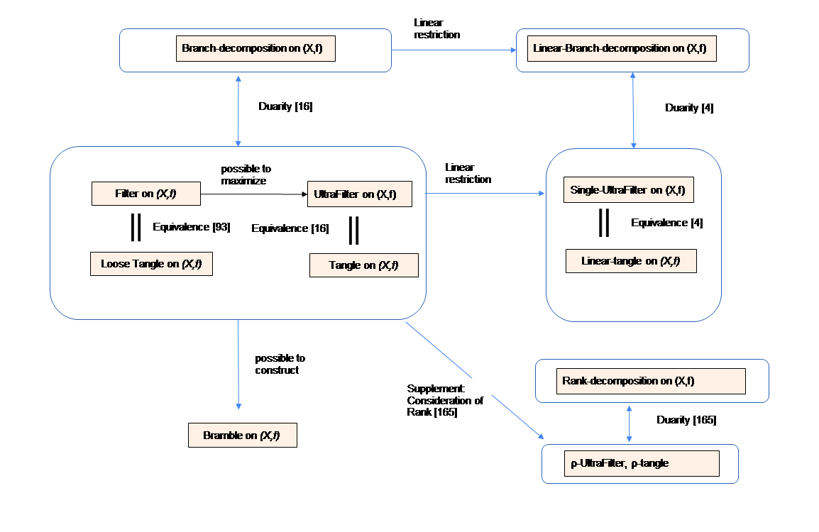
Figure 1: Relation about Width Parameter and Obstruction on Connectivity system

3 Tukey’s Lemma and Chain for Connectivity Systems

In this section, we explain some properties of ultrafilters on connectivity systems.

3.1 Chain for Connectivity Systems

First, let’s consider a chain on a connectivity system. Note that a chain in mathematics is crucial because it represents a totally ordered sequence of elements, which is fundamental in studying hierarchical structures, lattice theory, and optimization problems [64, 630, 262, 631, 472, 222, 416, 332].

Definition 3.1.

Let $X$ be a finite set and $f$ be a symmetric submodular function. A chain of order $k+1$ on a connectivity system is a sequence of subsets $\{A_{1},A_{2},\dots,A_{m}\}$ of $X$ such that:

1. $A_{1}\subseteq A_{2}\subseteq\dots\subseteq A_{m}$.

2. For each $i$ $(1\leq i\leq m)$, the symmetric submodular function $f$ evaluated at $A_{i}$ satisfies $f(A_{i})\leq k$.

3.2 Tukey’s Lemma for Connectivity System

We demonstrate the theorem (Tukey’s Lemma for Connectivity Systems) by using a chain of order $k+1$ on a connectivity system. Tukey’s Lemma states that in any non-empty collection of sets closed under taking supersets, there exists a maximal set within that collection. Intuitively, this means you can always find the largest possible set that cannot be expanded further while staying within the collection. Additionally, in set theory, Tukey’s Lemma is known to be closely related to Zorn’s Lemma (e.g., [618, 165, 66]). These lemmas are also widely recognized for their broad range of applications.

Theorem 3.2.

Let $X$ be a finite set and $f$ be a symmetric submodular function. Any filter on a connectivity system $(X,f)$, where $f$ is a symmetric submodular function and $X$ is a non-empty finite set, can be extended to an ultrafilter. Specifically, for any $k$-efficient subset $A\subseteq X$ (i.e., $f(A)\leq k$), there exists an ultrafilter containing the filter.

Proof 3.3.

Let $X$ be a finite set and $f$ be a symmetric submodular function. Here, we consider chains composed of $k$-efficient subsets.

First, we define the initial filter. Let $Q_{0}$ be a filter on the connectivity system $(X,f)$ where $f$ is a symmetric submodular function and $X$ is a non-empty finite set that satisfies the axioms $Q_{0}$ through $Q_{3}$.

Next, define the collection $\mathcal{F}$ as the set of all filters on $(X,f)$ that contain $Q_{0}$. This means $\mathcal{F}$ is the set of all sets $Q$ such that:

• $Q_{0}\subseteq Q$

• $Q$ satisfies axioms $Q_{0}$ through $Q_{3}$

$\mathcal{F}$ is partially ordered by inclusion. We need to show that every chain on $(X,f)$ (totally ordered subset on $(X,f)$) in $\mathcal{F}$ has an upper bound in $\mathcal{F}$.

Let $C\subseteq\mathcal{F}$ be a chain in $\mathcal{F}$, where each element of $C$ is a filter that respects the $k$-efficiency condition, meaning $f(A)\leq k$ for every $A$ in the filter.

Define $Q_{C}=\bigcup C$. We need to show that $Q_{C}$ is a filter and an element of $\mathcal{F}$.

Axiom (Q0): This axiom obviously holds.

Axiom (Q2): For any $A,B\in Q_{C}$, there exist $Q_{A},Q_{B}\in C$ such that $A\in Q_{A}$ and $B\in Q_{B}$. Since $C$ is a chain on the connectivity system, one of these filters contains the other; assume without loss of generality that $Q_{A}\subseteq Q_{B}$. Thus, $A,B\in Q_{B}$, and because $Q_{B}$ is a filter, $A\cap B\in Q_{B}\subseteq Q_{C}$. Additionally, since both $A$ and $B$ are in $Q_{C}$, $f(A)\leq k$ and $f(B)\leq k$ by Axiom (Q0). Therefore, $f(A\cap B)\leq k$ must hold because if it did not, $A\cap B$ would not be in $Q_{B}$, contradicting the closure under intersection in Axiom (Q1).

Axiom (Q1): For any $A\in Q_{C}$ and $A\subseteq B\subseteq X$, there exists $Q_{A}\in C$ such that $A\in Q_{A}$. Since $Q_{A}$ is a filter and $f(B)\leq k$, $B\in Q_{A}\subseteq Q_{C}$.

Axiom (Q3): Since $\emptyset\notin Q$ for any $Q\in C$, we have $\emptyset\notin Q_{C}$.

Thus, $Q_{C}$ is a filter on the connectivity system and $Q_{C}\in\mathcal{F}$.

$\mathcal{F}$ contains a maximal element $Q$. This maximal filter $Q$ satisfies axioms (Q0) through (Q3).

To show $Q$ is an ultrafilter, we need to verify Axiom (Q4): For any $A\subseteq X$ such that $f(A)\leq k$, suppose $A\notin Q$. We must show $X\setminus A\in Q$.

Assume $A\notin Q$. If $X\setminus A\notin Q$, then we will show that this leads to a contradiction, meaning $Q$ must contain either $A$ or $X\setminus A$.

1. Constructing $Q^{\prime}=Q\cup\{A\}$: If $A\notin Q$, consider adding $A$ to $Q$. This new set $Q^{\prime}=Q\cup\{A\}$ must be checked against the filter axioms.

2. Closed under Intersection: For $Q^{\prime}$, consider any $B\in Q$:

   • If $A$ were added to $Q$, $B\cap A$ might violate the $k$-efficiency condition. Specifically, since $A\notin Q$ and $Q$ is maximal, there could be an element $B\in Q$ such that $B\cap A$ does not satisfy $f(B\cap A)\leq k$. Since $B\cap A\notin Q$, this would violate Axiom (Q1), meaning $Q^{\prime}$ cannot be a filter.

3. Constructing $Q^{\prime\prime}=Q\cup\{X\setminus A\}$: If $X\setminus A\notin Q$, consider adding $X\setminus A$ to $Q$. This new set $Q^{\prime\prime}=Q\cup\{X\setminus A\}$ must also be checked against the filter axioms.

4. Closed under Intersection: For $Q^{\prime\prime}$, consider any $B\in Q$:

   • If $X\setminus A\notin Q$, then there must exist some $B\in Q$ such that $B\cap(X\setminus A)$ does not satisfy $f(B\cap(X\setminus A))\leq k$. Since $Q$ is maximal, adding $X\setminus A$ would create a set that fails to be closed under intersection, as $B\cap(X\setminus A)\notin Q$. This violates Axiom (Q1), meaning $Q^{\prime\prime}$ cannot be a filter.

Therefore, the assumption that both $A\notin Q$ and $X\setminus A\notin Q$ leads to contradictions. Hence, $Q$ must contain either $A$ or $X\setminus A$. This proof is completed.

We gain the following property of an ultrafilter on a connectivity system.

Theorem 3.4.

Let $X$ be a finite set and $f$ be a symmetric submodular function. In any finite non-empty connectivity system $(X,f)$ where $f$ is a symmetric submodular function, there exists at least one ultrafilter.

Proof 3.5.

Consider the collection $\mathcal{F}$ of all filters on $(X,f)$. This collection is non-empty because the trivial filter $\{X\}$ exists. By Tukey’s Lemma for Connectivity Systems, every filter can be extended to an ultrafilter. Thus, there exists at least one maximal element in $\mathcal{F}$ under inclusion that satisfies all the filter axioms and the ultrafilter condition $(Q4)$. This proof is completed.

3.3 Antichain for Connectivity Systems: Relationship among Ultrafilter, Chain, and Antichain

We consider an antichain on a connectivity system. An antichain is a collection of elements in a partially ordered set where no element is comparable to another, meaning no element in the set precedes or follows any other element in the ordering (cf. [64, 630, 262, 631, 472, 416, 332]).

Definition 3.6.

Let $X$ be a finite set and $f$ a symmetric submodular function. An antichain of order $k+1$ on a connectivity system is defined as a collection of subsets $\{A_{1},A_{2},\dots,A_{m}\}$ of $X$ such that:

1. Antichain Condition: For any two distinct subsets $A_{i}$ and $A_{j}$ in the collection, neither is a subset of the other, i.e., $A_{i}\not\subseteq A_{j}$ and $A_{j}\not\subseteq A_{i}$ for all $1\leq i,j\leq m$ with $i\neq j$.

2. Submodular Condition: For each $i$ $(1\leq i\leq m)$, the symmetric submodular function $f$ evaluated at $A_{i}$ satisfies $f(A_{i})\leq k$.

The relationship between chains and antichains is established by the following theorem. In this paper, the following theorem is called Dilworth’s Theorem [720, 69, 383, 672] on a connectivity system.

Theorem 3.7 (Dilworth’s Theorem for Connectivity Systems).

Let $(X,f)$ be a connectivity system with a symmetric submodular function $f$ and let $\mathcal{A}\subseteq 2^{X}$ be a family of subsets of $X$ such that $f(A)\leq k$ for all $A\in\mathcal{A}$. Then, the size of the largest antichain in $\mathcal{A}$ is equal to the minimum number of chains of order $k+1$ needed to cover $\mathcal{A}$.

Proof 3.8.

Let $X$ be a finite set and $f$ a symmetric submodular function. We proceed by induction on the number of elements in $X$.

For $|X|=1$, the statement trivially holds because any non-empty subset $\mathcal{A}$ of $X$ is both a chain and an antichain.

Assume the statement holds for all connectivity systems with less than $|X|$ elements. Consider a connectivity system $(X,f)$ with $|X|$ elements. Let $\mathcal{A}$ be a family of subsets of $X$ such that $f(A)\leq k$ for all $A\in\mathcal{A}$. We need to prove that the size of the largest antichain in $\mathcal{A}$ is equal to the minimum number of chains required to cover $\mathcal{A}$.

• Let $\mathcal{A}$ be an antichain such that no element in $\mathcal{A}$ is a subset of any other. Due to the submodularity condition, the maximum value of $f(A\cap B)$ for any $A,B\in\mathcal{A}$ is less than or equal to $k$, ensuring the sets in the antichain are maximally disconnected.

• Given any partition of $X$ into chains, by the pigeonhole principle, there is at least one element $A$ in $\mathcal{A}$ that intersects every chain. Each of these chains has an associated subset $A$ that satisfies $f(A)\leq k$, ensuring that the number of chains required to cover $\mathcal{A}$ is equal to the largest antichain.

By induction, the theorem holds for all finite connectivity systems. This proof is completed.

The relationship between ultrafilters and antichains is established by the following theorem.

Theorem 3.9.

Let $X$ be a finite set and $f$ be a symmetric submodular function. A maximal antichain on a connectivity system $(X,f)$ intersects with every ultrafilter of order $k+1$.

Proof 3.10.

Let $X$ be a finite set and $f$ a symmetric submodular function. Suppose $\{B_{1},B_{2},\dots,B_{n}\}$ is a maximal antichain of order $k+1$ on the connectivity system $(X,f)$. Let $U$ be an ultrafilter of order $k+1$ on $(X,f)$. Note that by definition, an ultrafilter $U$ satisfies: For any $A\subseteq X$ such that $f(A)\leq k$, either $A\in U$ or $X\setminus A\in U$ (this is the defining property of an ultrafilter on a connectivity system).

Now, consider each set $B_{i}$ in the antichain. Since $B_{i}$ are mutually incomparable and $f(B_{i})\leq k$ for all $i$, at least one of the sets $B_{i}$ must belong to the ultrafilter $U$, otherwise, the union $X\setminus\bigcup_{i=1}^{n}B_{i}$ would belong to $U$, which contradicts the maximality of the antichain (since $U$ would then not intersect with any $B_{i}$).

Hence, every ultrafilter of order $k+1$ intersects with the maximal antichain $\{B_{1},B_{2},\dots,B_{n}\}$. This proof is completed.

The relationship between ultrafilters and chains is established by the following theorem.

Theorem 3.11.

Let $X$ be a finite set and $f$ be a symmetric submodular function. In a chain of order $k+1$ on a connectivity system $(X,f)$, every ultrafilter of order $k+1$ contains exactly one set from the chain.

Proof 3.12.

Let $X$ be a finite set and $f$ a symmetric submodular function. Let $\{A_{1},A_{2},\dots,A_{m}\}$ be a chain of order $k+1$ on the connectivity system $(X,f)$, and let $U$ be an ultrafilter of order $k+1$ on $(X,f)$. By the properties of the chain, we have $A_{1}\subseteq A_{2}\subseteq\cdots\subseteq A_{m}$ with $f(A_{i})\leq k$ for each $i$. By the properties of the ultrafilter, for each set $A_{i}$, either $A_{i}\in U$ or $X\setminus A_{i}\in U$. Since the sets in the chain are nested, the ultrafilter cannot contain two different sets $A_{i}$ and $A_{j}$ with $i\neq j$ without violating the ultrafilter condition. Therefore, there must be a unique $A_{j}$ such that $A_{j}\in U$ and for all $i<j$, $A_{i}\notin U$. This proof is completed.

Theorem 3.13.

Let $(X,f)$ be a connectivity system with $X$ as a finite set and $f$ as a symmetric submodular function. The following holds:

1. Chain Extension: Every chain in the set of subsets of $X$, where $f(A)\leq k$ for all $A$ in the chain, can be extended to an ultrafilter on the connectivity system $(X,f)$.

2. Ultrafilter Inducing a Chain: Conversely, every ultrafilter on the connectivity system $(X,f)$ induces a maximal chain in the set of subsets of $X$.

Proof 3.14.

1. Chain Extension to Ultrafilter: Let $X$ be a finite set and $f$ a symmetric submodular function. Given a chain $C=\{A_{1}\subseteq A_{2}\subseteq\cdots\subseteq A_{m}\}$ where $f(A_{i})\leq k$ for each $i$, we want to show that this chain can be extended to an ultrafilter on the connectivity system $(X,f)$. Consider the filter $F$ generated by the chain $C$. This filter includes all supersets of elements in $C$ that satisfy $f(A)\leq k$. The symmetric submodular condition ensures that the intersection of any two sets in $F$ also belongs to $F$, maintaining the filter structure. By Theorem 3.2, this filter $F$ can be extended to a maximal filter, which is an ultrafilter $U$. This ultrafilter $U$ satisfies the condition that for any set $B\subseteq X$, either $B\in U$ or $X\setminus B\in U$, ensuring that $f(B)\leq k$ for all $B\in U$. Therefore, every chain $C$ in the set of subsets of $X$ can be extended to an ultrafilter $U$ on the connectivity system $(X,f)$.

2. Ultrafilter Inducing a Maximal Chain: Let $X$ be a finite set and $f$ a symmetric submodular function. Given an ultrafilter $U$ on the connectivity system $(X,f)$, we aim to show that $U$ induces a maximal chain in the set of subsets of $X$. For any set $A\in U$, consider the collection of subsets of $A$ that are also in $U$. This collection forms a chain because $U$ is a maximal filter, meaning that for any subset $A\subseteq B\subseteq X$, $B\in U$ if $A\in U$ and $f(B)\leq k$. The ultrafilter $U$ ensures that for any set $B\subseteq X$, either $B\in U$ or $X\setminus B\in U$, which means that the chain induced by $U$ cannot be extended further within $U$. This guarantees that the chain is maximal.

This proof is completed.

Theorem 3.15.

Let $X$ be a finite set and $f$ be a symmetric submodular function. In a chain of order $k+1$ on a connectivity system $(X,f)$, every ultrafilter of order $k$ does not contain a maximal set from the chain of order $k+1$.

Proof 3.16.

Consider a chain $\{A_{1}\subseteq A_{2}\subseteq\cdots\subseteq A_{m}\}$ in the connectivity system $(X,f)$, where $f(A_{i})\leq k$ for all $i$. This chain is said to be of order $k+1$ if $f(A_{i})\leq k$ for all sets in the chain. An ultrafilter of order $k$ on $(X,f)$ is a maximal filter where $f(A)<k$ for all $A$ in the ultrafilter. Suppose there exists an ultrafilter $U$ of order $k$ that contains the maximal set $A_{m}$ from the chain $\{A_{1}\subseteq A_{2}\subseteq\cdots\subseteq A_{m}\}$. Since $f$ is symmetric and submodular, $f(A_{m})\leq k$ holds because the chain is of order $k+1$. However, if $f(A_{m})=k$, then $A_{m}$ cannot belong to the ultrafilter $U$ of order $k$, because by definition, $U$ only contains sets where $f(A)<k$. This contradiction implies that the ultrafilter $U$ of order $k$ cannot contain the maximal set $A_{m}$. Therefore, every ultrafilter of order $k$ does not contain a maximal set from a chain of order $k+1$.

Theorem 3.17.

Let $X$ be a finite set and $f$ be a symmetric submodular function. In a chain of order $k$ on a connectivity system $(X,f)$, if no chain of order $k+1$ exists, then no ultrafilter of order $k+1$ exists.

Proof 3.18.

Let $\{A_{1}\subseteq A_{2}\subseteq\cdots\subseteq A_{m}\}$ be a chain of order $k$ in the connectivity system $(X,f)$, where $f(A_{i})\leq k$ for all $i$. Suppose no chain of order $k+1$ exists, meaning there is no set $A\subseteq X$ such that $f(A)\leq k$. Assume there exists an ultrafilter $U$ of order $k+1$ on $(X,f)$. By definition, an ultrafilter of order $k+1$ contains sets $B\subseteq X$ where $f(B)\leq k$. If such a set $B$ exists in $U$, then $B$ should be part of a chain of order $k+1$. However, since we assumed that no chain of order $k+1$ exists, no set $B\subseteq X$ can satisfy $f(B)\leq k$. This proof is completed.

In the future, we will consider the relationship between a chain on a connectivity system and branch-width on a connectivity system.

3.4 Sequence of connectivity system

Next, we consider about sequence chain (strong chain).

Definition 3.19.

Let $X$ be a finite set and $f$ be a symmetric submodular function. A sequence chain of order $k+1$ on a connectivity system $(X,f)$ is a sequence chain of subsets $\{A_{0},A_{1},\dots,A_{m}\}$ of $X$ such that:

1. $A_{0}=\emptyset$ and $A_{m}=X$.

2. $A_{0}\subseteq A_{1}\subseteq\dots\subseteq A_{m}$.

3. For each $i$ $(0\leq i\leq m)$, the symmetric submodular function $f$ evaluated at $A_{i}$ satisfies $f(A_{i})\leq k$.

Theorem 3.20.

Given a finite set $X$ and a symmetric submodular function $f:2^{X}\rightarrow\mathbb{N}$, if there exists a sequence chain $\{A_{0},A_{1},\dots,A_{m}\}$ of order $k+1$ on the connectivity system $(X,f)$, then no antichain of order $k+1$ can exist on the same system.

Proof 3.21.

Assume that there exists a sequence chain $\{A_{0},A_{1},\dots,A_{m}\}$ of order $k+1$ on the connectivity system $(X,f)$. By the definition of a sequence chain:

1. The sequence chain is a nested chain of subsets:

   $$A_{0}\subseteq A_{1}\subseteq\dots\subseteq A_{m},$$

   where $A_{0}=\emptyset$, $A_{m}=X$, and for each $i$, $f(A_{i})\leq k$.

Now, suppose, for the sake of contradiction, that an antichain $\{B_{1},B_{2},\dots,B_{n}\}$ of order $k+1$ also exists on the same connectivity system. By the definition of an antichain:

1. The antichain is a collection of subsets where no two distinct subsets are comparable by inclusion:

   $$B_{i}\not\subseteq B_{j}\text{ and }B_{j}\not\subseteq B_{i}\quad\text{for all }1\leq i,j\leq n,\ i\neq j,$$

   and for each $i$, $f(B_{i})\leq k$.

Since $\{A_{0},A_{1},\dots,A_{m}\}$ is a sequence chain, for each $B_{i}$ in the antichain, it must relate to the sets in the sequence chain in the following way:

• Comparability by Inclusion: Since the sequence chain $\{A_{0},A_{1},\dots,A_{m}\}$ is a chain, each $B_{i}$ in the antichain must be comparable by inclusion with each set in the sequence chain. Specifically, for each $B_{i}$, there must exist some $A_{j}$ in the sequence chain such that either: $B_{i}\subseteq A_{j}\quad\text{or}\quad A_{j}\subseteq B_{i}.$

  • If $B_{i}\subseteq A_{j}$: Then $B_{i}$ is contained within $A_{j}$, and since $A_{j}$ is part of the sequence chain, this violates the antichain condition because $B_{i}$ is now comparable to $A_{j}$ by inclusion.

  • If $A_{j}\subseteq B_{i}$: Then $A_{j}$ is contained within $B_{i}$, and similarly, this violates the antichain condition because $B_{i}$ is now comparable to $A_{j}$ by inclusion.

Given that the sequence chain imposes a strict order by inclusion on the subsets, any subset $B_{i}$ in the antichain would necessarily have to be either a subset of some $A_{j}$ or a superset of some $A_{j}$. This directly contradicts the requirement that no two distinct subsets in an antichain are comparable by inclusion.

Theorem 3.22.

Given a finite set $X$ and a symmetric submodular function $f:2^{X}\rightarrow\mathbb{N}$, if there exists a sequence chain $\{A_{0},A_{1},\dots,A_{m}\}$ of order $k+1$ on the connectivity system $(X,f)$, then no non-principal ultrafilter of order $k+1$ can exist on the same system.

Proof 3.23.

Since $F$ is a non-principal ultrafilter, it does not contain any singleton sets. Consider the following two cases:

• Case 1: $A_{i}\in F$ for some $A_{i}$ in the sequence chain.

  By the ultrafilter condition (Q4), since $A_{0}\subseteq A_{1}\subseteq\dots\subseteq A_{m}$ and $A_{i}\in F$, all supersets of $A_{i}$ must also be in $F$ (including $A_{m}=X$). However, $X$ cannot be in $F$ because $f(X)\leq k$ would imply that the entire set $X$ is part of the filter, which contradicts the non-principal nature of $F$, as non-principal filters do not include all of $X$ unless $X$ is trivial.

• Case 2: $A_{i}\notin F$ for all $A_{i}$ in the sequence chain.

  Since $A_{0}=\emptyset$ and $A_{m}=X$, by the ultrafilter condition (Q4), if $A_{i}\notin F$, then $X\setminus A_{i}\in F$. However, because the sequence chain is nested, if $A_{i}\notin F$, then $X\setminus A_{i}$ must be included in $F$. This contradicts the chain structure since, for some $j>i$, $A_{j}\subseteq X\setminus A_{i}$, and hence $A_{j}$ should be in $F$, contradicting the assumption that $A_{j}\notin F$.

Theorem 3.24.

Let $X$ be a finite set, and let $f:2^{X}\to\mathbb{N}$ be a symmetric submodular function. If there exists a sequence chain $\{A_{0},A_{1},\dots,A_{m}\}$ of order $k$ on the connectivity system $(X,f)$, then there exists a branch decomposition of the connectivity system $(X,f)$ with width at most $k$.

Proof 3.25.

Given the existence of a sequence chain $\{A_{0},A_{1},\dots,A_{m}\}$ of order $k$, we will construct a branch decomposition of $(X,f)$.

Start with a binary tree structure corresponding to the nested sequence chain $\{A_{0},A_{1},\dots,A_{m}\}$. For each subset $A_{i}$, assign a node $t_{i}$ in the tree such that $t_{0}$ corresponds to $A_{0}=\emptyset$, $t_{m}$ corresponds to $A_{m}=X$, and for all other $t_{i}$, $t_{i}$ corresponds to $A_{i}$.

Construct a tree $T$ such that each node $t_{i}$ is associated with a subset $A_{i}$ from the sequence chain. The leaves of $T$ are bijectively mapped to the elements of $X$. For every edge $e$ in $T$, define its width as the connectivity function $f$ evaluated on the set of vertices corresponding to the subtree induced by removing $e$ from $T$.

Since $f(A_{i})\leq k$ for each $i$, the width of each edge $e$ in the tree $T$ is at most $k$. Therefore, the branch-width of the constructed tree $(T,\mu)$ is at most $k$.

Theorem 3.26.

If there exists a sequence chain $\{A_{0},A_{1},\dots,A_{m}\}$ of order $k+1$ on the connectivity system $(X,f)$, then

• No antichain of order $k+1$ can exist.

• No non-principal ultrafilter of order $k+1$ can exist on the same system.

• No maximal ideal of order $k+1$ can exist on the same system [349].

• No tangle of order $k+1$ can exist on the same system [373].

• No (Maximal) loose tangle of order $k+1$ can exist on the same system [364].

• There exists a branch decomposition of the connectivity system $(X,f)$ with width at most $k$.

3.5 Other concepts on connectivity system

3.5.1 Separation chain on connectivity system

In graph theory, the concept of a separation chain is also utilized, particularly in proving graph width parameters such as path-width and cut-width[326, 732, 572]. We define the separation chain and separation sequence chain within a connectivity system. These concepts are essentially equivalent to their non-separation counterparts but incorporate the perspective of separations.

Definition 3.27.

Let $X$ be a finite set, and let $f:2^{X}\rightarrow\mathbb{N}$ be a symmetric submodular function. A separation chain of order $k+1$ on a connectivity system $(X,f)$ is a sequence of separations $\{(A_{1},B_{1}),(A_{2},B_{2}),\dots,(A_{m},B_{m})\}$ where $A_{i}\subseteq X$ and $B_{i}=X\setminus A_{i}$ for each $i$, such that:

1. $A_{1}\subseteq A_{2}\subseteq\dots\subseteq A_{m}$ and $B_{1}\supseteq B_{2}\supseteq\dots\supseteq B_{m}$.

2. For each $i$ $(1\leq i\leq m)$, the symmetric submodular function $f$ evaluated at $A_{i}$ satisfies $f(A_{i})\leq k$.

3. The width of the separation chain is defined as $\max_{1\leq i\leq m}|A_{i}\cap B_{i-1}|-1$.

Definition 3.28.

Let $X$ be a finite set, and let $f:2^{X}\rightarrow\mathbb{N}$ be a symmetric submodular function. A separation sequence chain of order $k+1$ on a connectivity system $(X,f)$ is a sequence of separations $\{(A_{0},B_{0}),(A_{1},B_{1}),\dots,(A_{m},B_{m})\}$ where $A_{i}\subseteq X$ and $B_{i}=X\setminus A_{i}$ for each $i$, such that:

1. $A_{0}=\emptyset$, $B_{0}=X$, $A_{m}=X$, and $B_{m}=\emptyset$.

2. $A_{0}\subseteq A_{1}\subseteq\dots\subseteq A_{m}$ and $B_{0}\supseteq B_{1}\supseteq\dots\supseteq B_{m}$.

3. For each $i$ $(0\leq i\leq m)$, the symmetric submodular function $f$ evaluated at $A_{i}$ satisfies $f(A_{i})\leq k$.

4. The width of the separation sequence chain is defined as $\max_{1\leq i\leq m}|A_{i}\cap B_{i-1}|-1$.

3.5.2 Sperner system on connectivity system

Concepts closely related to chains and antichains include the Sperner system and trace. We aim to explore the concept of a Sperner system within a connectivity system. A Sperner system is a collection of subsets where no subset is entirely contained within another. It is significant in combinatorics and other mathematical fields for studying set systems and their properties, such as in Boolean lattices and set theory [662, 428, 724, 374, 298, 682]. In set theory, a trace refers to the intersection of a set system with a subset, capturing how the system "traces" the structure of that subset [787, 772, 850, 724]. Although still in the conceptual stage, we outline the related definitions below.

Definition 3.29 (Sperner System on a Connectivity System).

Let $(X,f)$ be a connectivity system, where $X$ is a finite set and $f:2^{X}\rightarrow\mathbb{N}$ is a symmetric submodular function.

A Sperner system on $(X,f)$ is a collection $\mathcal{F}\subseteq 2^{X}$ such that there do not exist subsets $A,B\in\mathcal{F}$ with $A\subsetneq B$ and $f(A)\leq k$ and $f(B)\leq k$ for some $k$.

Definition 3.30 ($l$-Chain of Order $k+1$ on a Connectivity System).

An $l$-chain of order $k+1$ on a connectivity system $(X,f)$ is a subcollection $\{A_{1},A_{2},\dots,A_{l}\}\subseteq 2^{X}$ such that:

1. $A_{1}\subsetneq A_{2}\subsetneq\dots\subsetneq A_{l}$.

2. For each $i$ $(1\leq i\leq l)$, the symmetric submodular function $f$ evaluated at $A_{i}$ satisfies $f(A_{i})\leq k$.

Definition 3.31 ($l$-Sperner System on a Connectivity System).

An $l$-Sperner system on a connectivity system $(X,f)$ is a collection $\mathcal{F}\subseteq 2^{X}$ such that no $l$-chain of order $k+1$ exists within $\mathcal{F}$.

We say that an $l$-Sperner system on $(X,f)$ is saturated if, for every set $S\in 2^{X}\setminus\mathcal{F}$, the collection $\mathcal{F}\cup\{S\}$ contains an $l$-chain of order $k+1$ on $(X,f)$.

Definition 3.32 (Trace on a Connectivity System of Order $k+1$).

[724] Let $(X,f)$ be a connectivity system, where $X$ is a finite set and $f:2^{X}\rightarrow\mathbb{N}$ is a symmetric submodular function. For a set $F\subseteq 2^{X}$ and a subset $Y\subseteq X$, the trace of $F$ on $Y$ of order $k+1$ is defined as:

$$F|Y=\{F\cap Y:F\in F\text{ and }f(F\cap Y)\leq k\},$$

where $k$ is a fixed integer. This trace represents the collection of subsets of $Y$ formed by intersecting $Y$ with each subset in $F$, ensuring that the submodular function evaluated on these intersections remains within the desired bound.

Definition 3.33 (Strong Trace on a Connectivity System of Order $k+1$).

[724] A set $F\subseteq 2^{X}$ strongly traces a subset $Y\subseteq X$ of order $k+1$ if there exists a set $B\subseteq Y$ such that for any subset $Z\subseteq Y$, we have $B\cup Z\in F$ and $f(B\cup Z)\leq k$. The set $B$ is called the support of $Y$ by $F$, and the set of all such supports is denoted by $S_{F}(Y)$.

A concept related to the Sperner system is the clutter[517]. A clutter is a family of subsets (or hyperedges) in a hypergraph where no subset is contained within another, and it is frequently used in combinatorial optimization.

3.5.3 Chain-Decomposition on connectivity system

In the study of chains, concepts such as chain decomposition[834, 522], antichain decomposition[671, 279], and symmetric chains[33, 877, 854] have been extensively researched. These concepts are commonly utilized in partially ordered sets theory.

By adapting and defining these ideas within the context of connectivity systems, we aim to explore whether any interesting properties emerge. A chain decomposition breaks down a collection of subsets into disjoint chains. A symmetric chain extends the chain concept to include subsets of every size within a specified range, and a symmetric chain decomposition divides a collection into disjoint symmetric chains. An antichain decomposition partitions a collection into disjoint antichains. While still in the conceptual stage, the definitions are provided below.

Definition 3.34 (Disjoint Chains on a Connectivity System).

Two chains $\{A_{1},A_{2},\dots,A_{m}\}$ and $\{B_{1},B_{2},\dots,B_{n}\}$ on a connectivity system $(X,f)$ are said to be disjoint if no subset in one chain is a subset of any subset in the other chain. Formally, for all $i$ and $j$, $A_{i}\cap B_{j}=\emptyset$ or $A_{i}\not\subseteq B_{j}$ and $B_{j}\not\subseteq A_{i}$.

Definition 3.35 (Chain Decomposition on a Connectivity System).

A chain decomposition on a connectivity system $(X,f)$ is a partition of a collection of subsets $F\subseteq 2^{X}$ into disjoint chains of order $k+1$, where each chain satisfies the conditions specified in the chain definition.

Definition 3.36 (Symmetric Chain on a Connectivity System).

A symmetric chain on a connectivity system $(X,f)$ is a chain $\{A_{1},A_{2},\dots,A_{m}\}$ such that:

1. The chain contains subsets of every cardinality $i$ for $i\in\{k,k+1,\dots,|X|-k\}$, where $0\leq k\leq|X|/2$.

2. For each $i$ in the chain, the symmetric submodular function $f(A_{i})$ satisfies $f(A_{i})\leq k$.

Definition 3.37 (Symmetric Chain Decomposition on a Connectivity System).

A symmetric chain decomposition of a collection $F\subseteq 2^{X}$ on a connectivity system $(X,f)$ is a partition of $F$ into disjoint symmetric chains, where each symmetric chain satisfies the conditions specified in the symmetric chain definition.

Question 3.38.

How does the size of a symmetric chain relate to the order on a Connectivity System?

Definition 3.39 (Disjoint Antichains on a Connectivity System).

Two antichains $\{A_{1},A_{2},\dots,A_{m}\}$ and $\{B_{1},B_{2},\dots,B_{n}\}$ on a connectivity system $(X,f)$ are said to be disjoint if no subset in one antichain is a subset of any subset in the other antichain. Formally, for all $i$ and $j$, $A_{i}\cap B_{j}=\emptyset$ or $A_{i}\not\subseteq B_{j}$ and $B_{j}\not\subseteq A_{i}$.

Definition 3.40 (Antichain Decomposition on a Connectivity System).

An antichain decomposition on a connectivity system $(X,f)$ is a partition of a collection of subsets $F\subseteq 2^{X}$ into disjoint antichains of order $k+1$, where each antichain satisfies the conditions specified in the antichain definition.

3.5.4 Operation and Single-element-chain on a Connectivity System

In the future, we will delve into the concepts of operations and single-element-chains. We anticipate that the relationships observed between general chains, sequences, and ultrafilters will similarly apply to single-element structures, such as single-element-chains, single-element-sequences, single ultrafilters, and linear-width. The single-element extension (cf.[214, 210, 797, 816, 691]) on a connectivity system is also referred to as a one-point extension (cf.[589, 590]) or one-element lifting(cf.[381, 627, 382]) on the connectivity system. We also consider about single-element-coextension(cf.[685, 563, 808]) on a connectivity system.

Definition 3.41.

Given a chain $\{A_{1},A_{2},\dots,A_{m}\}$ of order $k+1$ on a connectivity system $(X,f)$, where $A_{1}\subseteq A_{2}\subseteq\dots\subseteq A_{m}$ and for each $i$, $f(A_{i})\leq k$:

1. Extension of the Chain: The extension of the chain by adding a new subset $A_{m+1}$ is defined as follows: Let $A_{m+1}\subseteq X$ be a subset such that $A_{m}\subseteq A_{m+1}$ and $f(A_{m+1})\leq k$. The resulting extended chain is $\{A_{1},A_{2},\dots,A_{m},A_{m+1}\}$.

2. Deletion of a Subset: The deletion of a subset $A_{i}$ from the chain is defined as follows: Remove $A_{i}$ from the chain, resulting in the chain $\{A_{1},\dots,A_{i-1},A_{i+1},\dots,A_{m}\}$. The condition that $f(A_{j})\leq k$ for all $j$ in the modified chain must still hold.

Definition 3.42.

A single-element-chain is a special case of a chain where each subset $A_{i}$ in the chain differs from the previous subset $A_{i-1}$ by exactly one element. Formally, a single-element-chain of order $k+1$ is defined as a sequence of subsets $\{A_{1},A_{2},\dots,A_{m}\}$ such that:

1. $A_{1}\subseteq A_{2}\subseteq\dots\subseteq A_{m}$.

2. For each $i$ $(1\leq i\leq m)$, $f(A_{i})\leq k$.

3. $|A_{i}\setminus A_{i-1}|=1$ for each $i$ $(2\leq i\leq m)$.

Definition 3.43.

A single-element-sequence chain is a specific type of sequence chain on a connectivity system $(X,f)$, where $f$ is a symmetric submodular function, and $X$ is a finite set. A single-element-sequence chain of order $k+1$ is defined as a sequence chain of subsets $\{A_{0},A_{1},\dots,A_{m}\}$ of $X$ such that:

1. $A_{0}=\emptyset$ and $A_{m}=X$.

2. $A_{0}\subseteq A_{1}\subseteq\dots\subseteq A_{m}$.

3. For each $i$ $(0\leq i\leq m)$, the symmetric submodular function $f$ evaluated at $A_{i}$ satisfies $f(A_{i})\leq k$.

4. For each $i$ $(1\leq i\leq m)$, $|A_{i}\setminus A_{i-1}|=1$, meaning that each subset $A_{i}$ in the sequence chain differs from the previous subset $A_{i-1}$ by exactly one element.

Definition 3.44.

The single-element-extension of a chain $\{A_{1},A_{2},\dots,A_{m}\}$ involves adding a new subset $A_{m+1}$ such that $A_{m+1}=A_{m}\cup\{e\}$, where $e\in X\setminus A_{m}$ and $f(A_{m+1})\leq k$. The new chain is $\{A_{1},A_{2},\dots,A_{m},A_{m+1}\}$.

Definition 3.45.

The single-element-deletion of a subset $A_{i}$ from the chain involves removing one element $e$ from $A_{i}$, resulting in $A_{i}^{\prime}=A_{i}\setminus\{e\}$. The new chain, after performing the deletion, must still satisfy the condition $f(A_{j})\leq k$ for all $j$. The resulting chain is $\{A_{1},\dots,A_{i-1},A_{i}^{\prime},A_{i+1},\dots,A_{m}\}$.

Definition 3.46.

Let $(X,f)$ be a connectivity system, and let ${A_{1},A_{2},\dots,A_{m}}$ be a chain of order $k+1$ within this system. Consider a set $X\cup{e}$, where $e\notin X$. The connectivity system $(X\cup{e},f^{\prime})$ is a single-element coextension of $(X,f)$ if for every subset $A\subseteq X$, the function $f^{\prime}$ satisfies $f^{\prime}(A)=f(A\cup{e})$. In this way, the function $f^{\prime}$ on the coextended system $(X\cup{e},f^{\prime})$ reduces to $f$ on the original system $(X,f)$ when the element $e$ is contracted.

4 Prefilter and Filter Subbase on a Connectivity System

We explain Prefilter and Filter Subbase on a connectivity system $(X,f)$. Prefilters and filter subbases, like ultrafilters, are crucial in set theory and topology for studying limits, convergence, and compactness. Prefilters are non-empty collections of sets closed under finite intersections, forming the basis for constructing filters. Filter subbases are non-empty collections of sets that generate filters by taking finite intersections, aiding in the study of convergence, limits, and compactness [844, 686, 318]. In this section, we add the condition of symmetric submodularity to prefilters and filter subbases and then perform verification.

4.1 Prefilter on a Connectivity System

First, we explain the definition of a prefilter and ultra-prefilter on a connectivity system $(X,f)$.

Definition 4.1.

Let $X$ be a finite set and $f$ be a symmetric submodular function. A prefilter of order $k+1$ on a connectivity system $(X,f)$ is a non-empty proper set family $P\subseteq 2^{X}$ that satisfies:

1. $\emptyset\notin P$ (Proper).

2. For any $A\in P$, $f(A)\leq k$ (k-efficiency).

3. For any $B,C\in P$, there exists some $A\in P$ such that $A\subseteq B\cap C$ and $f(A)\leq k$ (Downward Directed under k-efficiency).

Definition 4.2.

Let $X$ be a finite set and $f$ be a symmetric submodular function. An ultra-prefilter $P\subseteq 2^{X}$ on a connectivity system $(X,f)$ is a prefilter of order $k+1$ that satisfies the following additional property:

1. $\forall A\subseteq X,f(A)\leq k\Rightarrow\exists B\in P$ such that $B\subseteq A$ or $B\subseteq X\setminus A$ and $f(B)\leq k$.

Next, we demonstrate that a filter on a connectivity system can be considered a prefilter on that system. This concept extends the notions of prefilters and ultra-prefilters from set theory by incorporating the condition of symmetric submodularity.

Theorem 4.3.

Let $X$ be a finite set and $f$ be a symmetric submodular function. Any filter of order $k+1$ on a connectivity system $(X,f)$ is also a prefilter of order $k+1$ on the same connectivity system $(X,f)$.

Proof 4.4.

To prove that a filter $Q$ on a connectivity system is also a prefilter, we need to show that $Q$ satisfies all the conditions of a prefilter.

1. Axiom (P1): By definition, a filter $Q$ is non-empty because it contains subsets of $X$ that satisfy the given conditions. And by Axiom (Q3), $\emptyset\notin Q$. Therefore, $Q$ is a proper set family.

2. Axiom (P2): By Axiom (Q0), $\forall A\in Q,f(A)\leq k$. Therefore, every element in $Q$ satisfies the k-efficiency condition.

3. Axiom (P3): For any $B,C\in Q$ such that $f(B)\leq k$ and $f(C)\leq k$, we need to show there exists some $A\in Q$ such that $A\subseteq B\cap C$ and $f(A)\leq k$.

   • Given $B,C\in Q$, by Axiom (Q1), $f(B\cap C)\leq k\Rightarrow B\cap C\in Q$.

   • Since $B\cap C\in Q$ and by the definition of $Q$, $f(B\cap C)\leq k$, we can choose $A=B\cap C$.

   • Therefore, $A\in Q$, $A\subseteq B\cap C$, and $f(A)\leq k$.

Hence, $Q$ satisfies all the conditions of a prefilter. This proof is completed.

Next, we show that an ultrafilter on a connectivity system is also an ultra-prefilter on a connectivity system.

Theorem 4.5.

Let $X$ be a finite set and $f$ be a symmetric submodular function. Any ultrafilter of order $k+1$ on a connectivity system $(X,f)$ is also an ultra-prefilter of order $k+1$ on the same connectivity system $(X,f)$.

Proof 4.6.

Let $X$ be a finite set and $f$ be a symmetric submodular function. To prove that an ultrafilter $Q$ on a connectivity system is also an ultra-prefilter of order $k+1$ on a connectivity system, we need to show that $Q$ satisfies all the conditions of an ultra-prefilter of order $k+1$. Axioms (P1)-(P3) hold obviously. So we show that axiom (P4) holds.

For any $A\subseteq X$ such that $f(A)\leq k$, we need to show there exists some $B\in Q$ such that $B\subseteq A$ or $B\subseteq X\setminus A$ and $f(B)\leq k$. Given $A\subseteq X$ such that $f(A)\leq k$, by Axiom (Q4), either $A\in Q$ or $X\setminus A\in Q$. If $A\in Q$, then we can choose $B=A$, and $B\subseteq A$ with $f(B)\leq k$. If $X\setminus A\in Q$, then we can choose $B=X\setminus A$, and $B\subseteq X\setminus A$ with $f(B)\leq k$.

Hence, $Q$ satisfies all the conditions of an ultra-prefilter. This proof is completed.

4.2 Filter Subbase on a Connectivity System

Next, we introduce the definitions of filter subbase and ultrafilter subbase. These concepts extend the traditional notions of filter subbases and ultrafilter subbases from set theory by incorporating the condition of symmetric submodularity.

Definition 4.7.

Let $X$ be a finite set and $f$ be a symmetric submodular function. In a connectivity system $(X,f)$, a set family $S\subseteq 2^{X}$ is called a filter subbase of order $k+1$ if it satisfies the following conditions:

1. $S\neq\emptyset$.

2. $\emptyset\notin S$.

3. $\forall A\in S$, $f(A)\leq k$.

Definition 4.8.

Let $X$ be a finite set and $f$ be a symmetric submodular function. In a connectivity system $(X,f)$, a set family $S\subseteq 2^{X}$ is called an ultrafilter subbase of order $k+1$ if it satisfies the following conditions:

1. $S\neq\emptyset$.

2. $\emptyset\notin S$.

3. $\forall A\in S$, $f(A)\leq k$.

4. $\forall A\subseteq X$ such that $f(A)\leq k$, there exists $B\in S$ such that either $B\subseteq A$ or $B\subseteq X\setminus A$ and $f(B)\leq k$.

We now explore the relationship between a subbase on a connectivity system and a filter on a connectivity system. The following theorem establishes this relationship.

Theorem 4.9.

Let $X$ be a finite set and $f$ be a symmetric submodular function. Given a filter subbase $S$ of order $k+1$ on a connectivity system $(X,f)$, we can generate a filter $Q$ of order $k+1$ as follows: The filter $Q$ of order $k+1$ on a connectivity system $(X,f)$ generated by $S$ is the set of all subsets of $X$ that can be formed by finite intersections of elements of $S$. Formally,

$$Q=\{A\subseteq X\mid\exists A_{1},A_{2},\dots,A_{n}\in S\text{ such that }A=A_{1}\cap A_{2}\cap\dots\cap A_{n}\text{ and }f(A)\leq k\}.$$

Proof 4.10.

To prove that $Q$ is a filter of order $k+1$, we need to show that $Q$ satisfies the conditions of a filter of order $k+1$.

Axiom (Q0): This axiom obviously holds. By construction, every element in $Q$ is formed by finite intersections of elements in $S$. Since $S$ is a filter subbase of order $k+1$, all elements $A_{i}$ in $S$ satisfy $f(A_{i})\leq k$. By the submodularity of $f$, for any intersection $A=A_{1}\cap A_{2}\cap\dots\cap A_{n}$, we have $f(A)=f(A_{1}\cap A_{2}\cap\dots\cap A_{n})\leq\min(f(A_{1}),f(A_{2}),\dots,f(A_{n}))\leq k$.

Axiom (Q3): Since $S$ is a filter subbase of order $k+1$ on a connectivity system $(X,f)$, it is non-empty. Suppose $S=\{A_{1},A_{2},\dots,A_{m}\}$. Consider any single element $A_{i}\in S$. Since $S$ is non-empty, $A_{i}$ exists, and $f(A_{i})\leq k$. Therefore, $A_{i}\in Q$, implying $Q$ is non-empty. And by the definition of a filter subbase, $\emptyset\notin S$. Since $Q$ is generated by finite intersections of elements of $S$, and $\emptyset$ cannot be formed by any finite intersection of non-empty sets, $\emptyset\notin Q$. Therefore, $Q$ is proper.

Axiom (Q1): By construction, $Q$ consists of all subsets of $X$ that can be formed by finite intersections of elements of $S$ and satisfy $f(A)\leq k$. Thus, by definition, $Q$ satisfies the k-efficiency condition. Let $A,B\in Q$. Then there exist $A_{1},A_{2},\dots,A_{n}\in S$ and $B_{1},B_{2},\dots,B_{m}\in S$ such that $A=A_{1}\cap A_{2}\cap\dots\cap A_{n}$ and $f(A)\leq k$, $B=B_{1}\cap B_{2}\cap\dots\cap B_{m}$ and $f(B)\leq k$. Consider the intersection $A\cap B$:

$$A\cap B=(A_{1}\cap A_{2}\cap\dots\cap A_{n})\cap(B_{1}\cap B_{2}\cap\dots\cap B_{m}).$$

Since $S$ is a filter subbase and contains $A_{i}$ and $B_{j}$ for all $i,j$, $A\cap B$ is formed by the finite intersection of elements of $S$. Moreover, because $f$ is submodular and symmetric, $f(A\cap B)\leq\min(f(A),f(B))\leq k$. Thus, $A\cap B\in Q$.

Axiom (Q2): Let $A\in Q$ and $A\subseteq B\subseteq X$. By definition, there exist $A_{1},A_{2},\dots,A_{n}\in S$ such that $A=A_{1}\cap A_{2}\cap\dots\cap A_{n}$ and $f(A)\leq k$. If $f(B)\leq k$, we need to show $B\in Q$. Since $A\subseteq B$ and $f(B)\leq k$, $B$ can be considered as a superset satisfying the condition for being in $Q$.

Therefore, $Q$ is a filter of order $k+1$ generated by the filter subbase $S$. This proof is completed.

Theorem 4.11.

Let $X$ be a finite set and $f$ be a symmetric submodular function. Given a filter subbase $S$ of order $k+1$ on a connectivity system $(X,f)$, we can generate a prefilter $Q$ of order $k+1$ as follows:

$$Q=\{A\subseteq X\mid\exists A_{1},A_{2},\dots,A_{n}\in S\text{ such that }A=A_{1}\cap A_{2}\cap\dots\cap A_{n}\text{ and }f(A)\leq k\}.$$

Proof 4.12.

To demonstrate that $Q$ is a prefilter of order $k+1$, we need to verify that $Q$ satisfies the conditions of a prefilter as defined by axioms (P1) to (P3).

Axiom (P1): Since $S$ is a non-empty filter subbase, by definition, $S$ does not contain $\emptyset$. $Q$ is formed by finite intersections of elements in $S$, and because $\emptyset$ cannot be formed by such intersections, $\emptyset\notin Q$. Therefore, $Q$ is proper and non-empty, satisfying axiom (P1).

Axiom (P2): By construction, each element $A\in Q$ is the intersection of a finite number of sets $A_{1},A_{2},\dots,A_{n}\in S$ such that $f(A)\leq k$. Since $S$ is a filter subbase of order $k+1$, all elements $A_{i}\in S$ satisfy $f(A_{i})\leq k$. The submodularity of function $f$ ensures that $f(A_{1}\cap A_{2}\cap\dots\cap A_{n})\leq\min(f(A_{1}),f(A_{2}),\dots,f(A_{n}))\leq k$. Therefore, every element $A\in Q$ satisfies $f(A)\leq k$, ensuring k-efficiency as required by axiom (P2).

Axiom (P3): For any $B,C\in Q$, there exist sets $B_{1},B_{2},\dots,B_{m}\in S$ and $C_{1},C_{2},\dots,C_{n}\in S$ such that $B=B_{1}\cap B_{2}\cap\dots\cap B_{m}$ and $C=C_{1}\cap C_{2}\cap\dots\cap C_{n}$, with $f(B)\leq k$ and $f(C)\leq k$. Consider the intersection $A=B\cap C$. Since $A=(B_{1}\cap B_{2}\cap\dots\cap B_{m})\cap(C_{1}\cap C_{2}\cap\dots\cap C_{n})$, $A$ is formed by a finite intersection of elements in $S$. The submodularity and symmetry of function $f$ imply that $f(A)=f(B\cap C)\leq\min(f(B),f(C))\leq k$. Therefore, $A\in Q$, satisfying axiom (P3).

Given that $Q$ satisfies all the conditions (P1)-(P3) of a prefilter, we conclude that $Q$ is indeed a prefilter of order $k+1$ generated by the filter subbase $S$. This completes the proof.

Theorem 4.13.

Let $X$ be a finite set and $f$ be a symmetric submodular function. Given an ultrafilter subbase $S$ of order $k+1$ on a connectivity system $(X,f)$, we can generate an ultrafilter $Q$ of order $k+1$ as follows: The filter $Q$ of order $k+1$ on a connectivity system $(X,f)$ generated by $S$ is the set of all subsets of $X$ that can be formed by finite intersections of elements of $S$. Formally,

$$Q=\{A\subseteq X\mid\exists A_{1},A_{2},\dots,A_{n}\in S\text{ such that }A=A_{1}\cap A_{2}\cap\dots\cap A_{n}\text{ and }f(A)\leq k\}.$$

Proof 4.14.

The proof can be established using a method nearly identical to that used in Theorem 4.9. This completes the proof.

Theorem 4.15.

Let $X$ be a finite set and $f$ be a symmetric submodular function. Given an ultrafilter subbase $S$ of order $k+1$ on a connectivity system $(X,f)$, we can generate an ultra-prefilter $Q$ of order $k+1$ as follows:

$$Q=\{A\subseteq X\mid\exists A_{1},A_{2},\dots,A_{n}\in S\text{ such that }A=A_{1}\cap A_{2}\cap\dots\cap A_{n}\text{ and }f(A)\leq k\}.$$

Proof 4.16.

The proof can be established using a method nearly identical to that used in Theorem 4.11. This completes the proof.

Based on the above, the relationships shown in the following diagram become clear.

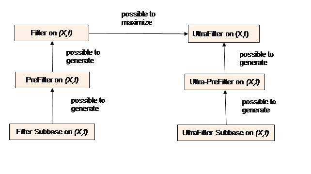
Figure 2: Relation about generating a filter

4.3 Ultrafilter Number

In set theory and various mathematical fields, the concept of the Ultrafilter Number (Cardinality) is frequently discussed (ex.[406, 745, 166]). We plan to explore whether this can be extended to Connectivity Systems and, if so, what characteristics can be derived from such an extension.

Definition 4.17 (Ultrafilter Number on a Connectivity System).

Let $(X,f)$ be a finite connectivity system, where $X$ is a finite set and $f:2^{X}\rightarrow\mathbb{N}$ is a symmetric submodular function. The Ultrafilter Number $u(X,f)$ on this connectivity system is defined as the minimum size of a set $B\subseteq X$ such that $B$ forms a ultra prefilter for a non-principal ultrafilter on $(X,f)$. Formally,

$$u(X,f)=\min\{|B|:B\text{ is a ultra prefilter for a non-principal ultrafilter on }(X,f)\}.$$

Question 4.18.

How does the Ultrafilter Number relate to the order on a Connectivity System?

5 Ultrafilter on Infinite Connectivity System and Countable Connectivity System

5.1 Ultrafilter on Infinite Connectivity System

Until now, we have considered ultrafilters on finite sets, but now we turn our attention to ultrafilters on infinite sets. First, let’s define what an infinite connectivity system is.

Definition 5.1 ([157, 290, 205]).

Consider an infinite set $X$ equipped with a symmetric submodular function $f$ mapping from the set of subsets of $X$ to $\mathbb{N}\cup\{\infty\}$. This function satisfies the following conditions for all subsets $A$ and $B$ of $X$:

1. Symmetry: $f(A)=f(X\setminus A)$.

2. Submodularity: $f(A)+f(B)\geq f(A\cup B)+f(A\cap B)$.

In the context of infinite sets, we also require $f$ to be $k$-limit-closed. Specifically, if $k\in\mathbb{N}$ and $(A_{i})_{i\in I}$ is a chain of subsets of $X$ each with connectivity at most $k$, then the union $\bigcup_{i\in I}A_{i}$ also has connectivity at most $k$. It is important to note that the ground set of a (possibly infinite) matroid, along with its connectivity function, constitutes a connectivity system, and the connectivity function is defined to be $k$-limit-closed. A pair $(X,f)$ is called an infinite connectivity system.

Given the known lemma, it is reasonable to consider a deep relationship between finite sets and infinite sets.

Lemma 5.2 ([157]).

Let $X$ be an infinite set and $f$ be a symmetric submodular function. Let $k\in\mathbb{N}$, and let $A\subseteq X$ be a set such that all finite subsets have connectivity at most $k$. Then also $f(A)\leq k$.

Following the model of ultrafilters on finite sets, we define ultrafilters on infinite sets as follows [373].

Definition 5.3 (cf. [373]).

Let $X$ be an infinite set and $f$ be a symmetric submodular function. In an infinite connectivity system $(X,f)$, the set family $F\subseteq 2^{X}$ is called a filter of order $k+1$ if the following axioms hold true:

1. $\forall A\in F,f(A)\leq k$.

2. $A\in F,B\in F,f(A\cap B)\leq k\Rightarrow A\cap B\in F$.

3. $A\in F,A\subseteq B\subseteq X,f(B)\leq k\Rightarrow B\in F$.

4. $\emptyset\notin F$.

An ultrafilter of order $k+1$ on an infinite connectivity system $(X,f)$ is a filter of order $k+1$ on an infinite connectivity system $(X,f)$ which satisfies the following additional axiom:

1. $\forall A\subseteq X,f(A)\leq k\Rightarrow\text{either }A\in F\text{ or }X\setminus A\in F$.

A filter of order $k+1$ on an infinite connectivity system $(X,f)$ is principal if the filter satisfies the following axiom [373]:

1. $A\in F$ for all $A\subseteq X$ with $|A|=1$ and $f(A)\leq k$.

A filter of order $k+1$ on an infinite connectivity system $(X,f)$ is non-principal if the filter satisfies the following axiom [373]:

1. $A\notin F$ for all $A\subseteq X$ with $|A|=1$.

Non-principal refers to a filter or ideal that does not contain any singletons (i.e., sets with exactly one element).

If a filter on an infinite connectivity system is weak [351, 591, 44], the following axiom holds instead of axiom (Q1):

1. $A\in F,B\in F,f(A\cap B)\leq k\Rightarrow A\cap B\neq\emptyset$.

Note that weak filters aim at interpreting defaults via a generalized ‘most’ quantifier in first-order logic [591, 44, 775, 336]. A weak filter on an infinite connectivity system is a co-Weak Ideal on an infinite connectivity system.

If a filter on an infinite connectivity system is quasi [359, 176], the following axiom holds instead of axiom (Q1):

1. $A\subseteq X,B\subseteq X,A\notin F,B\notin F\Rightarrow A\cup B\notin F$.

Note that a quasi-Ultrafilter is used to perform an axiomatic analysis of incomplete social judgments [176].

The following also holds for infinite connectivity systems, just as it does for finite connectivity systems.

Theorem 5.4.

Consider an infinite set $X$ equipped with a symmetric submodular function $f:2^{X}\to\mathbb{N}\cup\{\infty\}$. Note that Limit-Closed means that for any $k\in\mathbb{N}$ and any chain $(A_{i})_{i\in I}$ of subsets of $X$, each with connectivity at most $k$, the union $\bigcup_{i\in I}A_{i}$ also has connectivity at most $k$. An ultrafilter of order $k+1$ on an infinite connectivity system $(X,f)$ is also an ultrafilter of order $k$ on an infinite connectivity system $(X,f)$.

Proof 5.5.

By using the symmetric submodular function, an ultrafilter of order $k+1$ on an infinite connectivity system $(X,f)$ obviously holds the axioms of an ultrafilter of order $k$ on an infinite connectivity system $(X,f)$. This proof is completed.

Here are some properties that hold for filters and ultrafilters of order $k+1$ on an infinite connectivity system.

Lemma 5.6.

Consider an infinite set $X$ equipped with a symmetric submodular function $f:2^{X}\to\mathbb{N}\cup\{\infty\}$. Suppose an infinite connectivity system $(X,f)$ satisfies $k$-Limit-Closed. If a filter of order $k+1$ on an infinite connectivity system $(X,f)$ is maximal, it satisfies the following additional axiom:

• $\forall A\subseteq X$, if $f(A)\leq k$, then either $A\in F$ or $X\setminus A\in F$.

Proof 5.7.

Assume that there exists a maximal filter $F$ of order $k+1$ on $(X,f)$ that does not satisfy axiom (Q4). That is, there exists a subset $A\subseteq X$ such that $f(A)\leq k$, but neither $A\in F$ nor $X\setminus A\in F$. Since $F$ is maximal, the addition of $A$ or $X\setminus A$ to $F$ would result in a filter that still respects the conditions of $f(A)\leq k$. Therefore, $F\cup\{A\}$ or $F\cup\{X\setminus A\}$ would also be a valid filter, contradicting the maximality of $F$. Thus, the assumption that $F$ does not satisfy (Q4) leads to a contradiction. Therefore, any maximal filter $F$ of order $k+1$ must satisfy axiom (Q4). This proof is completed.

Definition 5.8 (cf. [312]).

Consider an infinite set $X$ equipped with a symmetric submodular function $f:2^{X}\to\mathbb{N}\cup\{\infty\}$. We will say that a family $F$ of order $k+1$ on an infinite connectivity system is nice if it is nonempty, closed under intersections (i.e., if $A,B\in F$ and $f(A\cap B)\leq k$, then $A\cap B\in F$), and $\emptyset\notin F$.

Lemma 5.9.

Consider an infinite set $X$ equipped with a symmetric submodular function $f:2^{X}\to\mathbb{N}\cup\{\infty\}$. Suppose an infinite connectivity system $(X,f)$ satisfies $k$-Limit-Closed. A family of subsets of $X$ is maximal nice of order $k+1$ on an infinite connectivity system if and only if it is an ultrafilter of order $k+1$ on an infinite connectivity system.

Proof 5.10.

Let’s first recall that a family $F$ of order $k+1$ on an infinite connectivity system is called nice if it is nonempty, closed under intersections (i.e., if $A,B\in F$ and $f(A\cap B)\leq k$, then $A\cap B\in F$), and $\emptyset\notin F$.

Assume that $F$ is a maximal nice family of order $k+1$. We want to show that $F$ is an ultrafilter of order $k+1$, i.e., it satisfies axiom (Q4): $\forall A\subseteq X$, if $f(A)\leq k$, then either $A\in F$ or $X\setminus A\in F$. Suppose $F$ is maximal nice, but there exists a subset $A\subseteq X$ such that $f(A)\leq k$, and neither $A\in F$ nor $X\setminus A\in F$. Since $F$ is maximal, we can extend $F$ by adding either $A$ or $X\setminus A$ to form a new family $F^{\prime}$. But this contradicts the maximality of $F$, as it can still be extended. Therefore, $F$ must satisfy (Q4), and hence it is an ultrafilter of order $k+1$.

Now assume $F$ is an ultrafilter of order $k+1$. We need to show that $F$ is maximal nice. Suppose $F$ is not maximal nice. Then there exists a family $F^{\prime}$ such that $F\subsetneq F^{\prime}$ and $F^{\prime}$ is nice. But since $F$ is an ultrafilter, it cannot be extended by adding more sets without violating the conditions for an ultrafilter. This contradicts the assumption that $F$ is not maximal nice. Hence, $F$ must be maximal nice. This proof is completed.

In this paper, let $\text{Fr}=\{A\subseteq X\mid f(A)\leq k,X\setminus A\text{ is finite}\}$ be the Frechet filter of order $k+1$ on an infinite connectivity system $(X,f)$. We consider the following lemma.

Lemma 5.11.

Consider an infinite set $X$ equipped with a symmetric submodular function $f:2^{X}\to\mathbb{N}\cup\{\infty\}$. Suppose an infinite connectivity system $(X,f)$ satisfies $k$-Limit-Closed. If there exists a Frechet filter of order $k+1$ on an infinite connectivity system $(X,f)$, then there exists a nonprincipal ultrafilter of order $k+1$ on an infinite connectivity system $(X,f)$.

Proof 5.12.

Assume that there does not exist a nonprincipal ultrafilter of order $k+1$ on $(X,f)$. This implies that every ultrafilter on $(X,f)$ must be principal. If Fr can be extended to an ultrafilter, this ultrafilter would be principal. A principal ultrafilter contains a set $\{x\}$ for some $x\in X$ with $f(\{x\})\leq k$. However, by definition, in a Frechet filter, $X\setminus\{x\}$ is finite, and thus $X$ cannot have only principal ultrafilters if it contains elements for which $f(\{x\})\leq k$. This contradicts the assumption that every ultrafilter is principal. Thus, there must exist a nonprincipal ultrafilter of order $k+1$ on $(X,f)$. This proof is completed.

We consider the following extended Ramsey’s Theorem on an infinite connectivity system. Note that Ramsey’s Theorem states that for any given positive integers $k$ and $r$, there is a minimum number $R(k,r)$ such that any graph with $R(k,r)$ vertices, colored with $r$ colors, contains a monochromatic clique of size $k$. Note that a monochromatic clique is a subset of vertices where all edges connecting them are the same color. This theorem can also be considered in terms of partitions, ensuring any partition of edges or vertices leads to a monochromatic subset.

Theorem 5.13.

Consider an infinite set $X$ equipped with a symmetric submodular function $f:2^{X}\to\mathbb{N}\cup\{\infty\}$. Suppose an infinite connectivity system $(X,f)$ satisfies $k$-Limit-Closed. Then for any infinite partition $P=\{A_{1},A_{2},\dots\}$ of $X$, there exists an infinite subset $Y\subseteq X$ such that all subsets of $Y$ are contained within a single block of the partition and have connectivity at most $k$.

Proof 5.14.

Let $X$ be an infinite set with the symmetric submodular function $f$ as defined. Let $P=\{A_{1},A_{2},\dots\}$ be a partition of $X$. We want to find an infinite subset $Y\subseteq X$ such that all subsets of $Y$ are contained within a single block of $P$ and have connectivity at most $k$.

Consider an increasing chain of subsets $(A_{i})_{i\in I}$ of $X$, where each $A_{i}$ has connectivity at most $k$. By the limit-closed property of function $f$, the union $\bigcup_{i\in I}A_{i}$ also has connectivity at most $k$.

Using the classical form of Ramsey’s Theorem, we know that for any infinite set $X$ and any partition of $X$ into finitely many pieces, there exists an infinite subset $Y\subseteq X$ such that all pairs in $Y$ lie within the same piece of the partition. To apply Ramsey’s Theorem in the context of the connectivity system $(X,f)$, we need to ensure that the infinite subset $Y$ not only lies within a single block of the partition but also maintains the connectivity condition $f(Y)\leq k$.

Start with an infinite subset $Y_{0}\subseteq X$. Partition $Y_{0}$ into blocks $A_{i}$ according to the given partition $P$. Select a block $A_{j}$ that contains an infinite subset $Y_{1}\subseteq A_{j}$. By the symmetry and submodularity of function $f$, ensure $f(Y_{1})\leq k$.

By iterating the process, we can construct a nested sequence of infinite subsets $Y_{0}\supseteq Y_{1}\supseteq Y_{2}\supseteq\dots$, each lying within a single block of the partition and maintaining the connectivity condition $f(Y_{i})\leq k$.

Let $Y=\bigcap_{i=0}^{\infty}Y_{i}$. Since each $Y_{i}$ is infinite and lies within a single block of the partition, $Y$ is also infinite and lies within a single block of the partition. Moreover, by the limit-closed property of the infinite connectivity system, we obtain $f(Y)\leq k$.

Thus, we have shown that for any infinite partition $P$ of $X$, there exists an infinite subset $Y\subseteq X$ such that all subsets of $Y$ lie within a single block of the partition and have connectivity at most $k$. This completes the proof of the extended Ramsey’s Theorem on an infinite connectivity system.

Theorem 5.15.

Let $(X,f)$ be an infinite connectivity system with $f$ a symmetric submodular function satisfying $k$-Limit-Closed. A set family $U\subseteq 2^{X}$ is a weak ultrafilter of order $k+1$ if and only if it is a maximal weak filter of order $k+1$ on $(X,f)$.

Proof 5.16.

Assume that $U$ satisfies the definition of a weak ultrafilter but is not maximal. This means there exists a weak filter $G$ such that $U\subset G$ and $G$ contains an additional set $A\subset X$ where $A\in G$ but $A\notin U$. Since $U$ is a weak ultrafilter, by its definition, for any subset $A\subseteq X$ with $f(A)\leq k$, it must hold that either $A\in U$ or $X\setminus A\in U$.

Now, because $U\subset G$, every element of $U$ is also an element of $G$. Specifically, since $X\setminus A\in U$ and $U\subset G$, it follows that $X\setminus A$ must also be in $G$. However, $G$ already contains $A$ by assumption, and now it also contains $X\setminus A$. For $G$ to be a consistent weak filter, it cannot contain both $A$ and $X\setminus A$ because that would violate the condition of non-empty intersection. This leads to a contradiction because if $G$ contains both $A$ and $X\setminus A$, it would mean that $G$ is no longer a valid weak filter due to inconsistency, which contradicts the assumption that $G$ is a weak filter.

Hence, $U$ must be maximal because extending $U$ to any larger set $G$ results in an inconsistency, proving that $U$ cannot be properly contained in any larger weak filter.

We need to prove that $U$ is a weak ultrafilter of order $k+1$. Specifically, for any subset $A\subset X$ with $f(A)\leq k$ and $A\notin U$, we must show $X\setminus A\in U$.

Let $G$ be the upward closure of $U\cup\{A\}$, meaning $G$ includes all sets in $U$ as well as any sets that can be formed by taking unions of elements from $U$ and $A$.

By the assumption that $U$ is maximal, $G$ cannot form a weak filter. If $G$ were a weak filter, it would contradict the maximality of $U$.

The fact that $G$ cannot be a weak filter means that there must exist some set $Z\subseteq X$ in $G$ such that $Z\supset A$, and for some $Y\in U$, we have $Z\cap Y=\emptyset$. This condition arises because if $Z$ and $Y$ were both in $G$, it would imply that $Z$ and $Y$ must intersect, which they do not in this scenario.

The existence of such a $Z$ means that the complement $X\setminus A$ must be in $U$ to maintain the weak ultrafilter property (since $U$ must contain the complement if it does not contain the original set).

This confirms that $U$ must contain $X\setminus A$, proving that $U$ behaves like a weak ultrafilter of order $k+1$. This proof is completed.

In the future, we plan to further investigate the theorems related to ultrafilters on infinite connectivity systems. For example, we will consider the following definitions of Selective and Weakly Selective Ultrafilters on a Connectivity System (cf. [100, 97, 328, 167]).

Definition 5.17.

Consider an infinite set $X$ equipped with a symmetric submodular function $f:2^{X}\to\mathbb{N}\cup\{\infty\}$. Suppose an infinite connectivity system $(X,f)$ satisfies $k$-Limit-Closed. Assume that for all $x\in X$, $f(\{x\})\leq k$. An ultrafilter $F$ on $(X,f)$ is called selective if for every function $g:X\to X$, there exists a subset $A\in F$ such that $g\mid A$ is either:

• Constant: $g(x)=c$ for all $x\in A$, or

• One-to-One: $g(x_{1})\neq g(x_{2})$ for all distinct $x_{1},x_{2}\in A$.

Definition 5.18.

Consider an infinite set $X$ equipped with a symmetric submodular function $f:2^{X}\to\mathbb{N}\cup\{\infty\}$. Suppose an infinite connectivity system $(X,f)$ satisfies $k$-Limit-Closed. An ultrafilter $F$ on $(X,f)$ is called quasi-selective if for every function $g:X\to X$ with $g(x)\leq x$ for all $x\in X$ where $f(\{x\})\leq k$, there exists a subset $A\in F$ such that $g\mid A$ is a non-decreasing function.

5.1.1 P-point and Q-point on an infinite connectivity system

A P-Point is an ultrafilter such that for any partition of a set into subsets not in the ultrafilter, there exists a subset with finite intersections. A Q-Point is an ultrafilter where, for any partition of a set into finite pieces, there exists a subset with intersections of at most one element. P-Points and Q-Points are studied in fields such as topology [98, 215, 731, 657]. We explore P-Points and Q-Points within the context of an infinite connectivity system.

Definition 5.19.

Consider an infinite set $X$ equipped with a symmetric submodular function $f:2^{X}\to\mathbb{N}\cup\{\infty\}$. Suppose an infinite connectivity system $(X,f)$ satisfies $k$-Limit-Closed. Additionally, let $\{X_{n}\}_{n<\omega}$ be a symmetric submodular partition of $X$ such that $f(X_{n})\leq k$ for all $n$.

Ramsey (Selective) Point of Order $k+1$: A subset $A\subseteq X$ is called a Ramsey Point of order $k+1$ if for every symmetric submodular partition $\{X_{n}\}_{n<\omega}$ of $X$ such that $f(X_{n})\leq k$ and $X_{n}\notin F$ for all $n$, there exists an $A\in F$ such that:

$$|A\cap X_{n}|\leq 1,\quad f(A\cap X_{n})\leq k,\quad\text{and}\quad f(A)\leq k\quad\text{for all }n<\omega.$$

P-Point (Weakly Selective Point) of Order $k+1$: A subset $A\subseteq X$ is called a P-Point of order $k+1$ if for every symmetric submodular partition $\{X_{n}\}_{n<\omega}$ of $X$ such that $f(X_{n})\leq k$ and $X_{n}\notin F$ for all $n$, there exists an $A\in F$ such that:

$$|A\cap X_{n}|<\omega,\quad f(A\cap X_{n})\leq k,\quad\text{and}\quad f(A)\leq k\quad\text{for all }n<\omega.$$

Q-Point of Order $k+1$: A subset $A\subseteq X$ is called a Q-Point of order $k+1$ if for every symmetric submodular partition $\{X_{n}\}_{n<\omega}$ of $X$ into finite sets, such that $f(X_{n})\leq k$ and $X_{n}\notin F$ for all $n$, there exists an $A\in F$ such that:

$$|A\cap X_{n}|\leq 1,\quad f(A\cap X_{n})\leq k,\quad\text{and}\quad f(A)\leq k\quad\text{for all }n<\omega.$$

Semi-Q-Point (Rapid Point) of Order $k+1$: A subset $A\subseteq X$ is called a Semi-Q-Point of order $k+1$ if for every symmetric submodular partition $\{X_{n}\}_{n<\omega}$ of $X$ into finite sets, such that $f(X_{n})\leq k$ and $X_{n}\notin F$ for all $n$, there exists an $A\in F$ such that:

$$|A\cap X_{n}|\leq n,\quad f(A\cap X_{n})\leq k,\quad\text{and}\quad f(A)\leq k\quad\text{for all }n<\omega.$$

Theorem 5.20.

Consider an infinite set $X$ equipped with a symmetric submodular function $f:2^{X}\to\mathbb{N}\cup\{\infty\}$. Suppose an infinite connectivity system $(X,f)$ satisfies $k$-Limit-Closed. An ultrafilter $F$ on an infinite connectivity system $(X,f)$ is Ramsey (Selective) of order $k+1$ if and only if it is both a P-Point and a Q-Point of order $k+1$.

Proof 5.21.

Assume $F$ is a Ramsey ultrafilter of order $k+1$. By definition:

1. Since $F$ is Ramsey, for every symmetric submodular partition $\{X_{n}\}_{n<\omega}$ of $X$, there exists an $A\in F$ such that $|A\cap X_{n}|\leq 1$ and $f(A\cap X_{n})\leq k$ for all $n<\omega$.

   • This directly implies that $A$ also satisfies the conditions for a Q-Point, as it meets the finite intersection condition $|A\cap X_{n}|\leq 1$.

2. Similarly, the condition $|A\cap X_{n}|\leq 1$ (from being Ramsey) trivially implies $|A\cap X_{n}|<\omega$, satisfying the requirement for a P-Point.

Thus, every Ramsey ultrafilter of order $k+1$ is also a P-Point and a Q-Point of the same order.

Now, assume $F$ is both a P-Point and a Q-Point of order $k+1$. We need to show that $F$ is Ramsey of order $k+1$.

Let $\{X_{n}\}_{n<\omega}$ be a symmetric submodular partition of $X$ such that $X_{n}\notin F$ and $f(X_{n})\leq k$ for all $n$.

1. Since $F$ is a P-Point of order $k+1$, we can choose a set $A_{0}\in F$ such that $|A_{0}\cap X_{n}|<\omega$ and $f(A_{0}\cap X_{n})\leq k$ for all $n<\omega$.

2. Enumerate the elements of $X\setminus\bigcup_{n<\omega}(A_{0}\cap X_{n})=\{a_{n}\}_{n<\omega}$ and define new sets $Y_{2n}:=A_{0}\cap X_{n}$ and $Y_{2n+1}:=\{a_{n}\}$.

3. Since $F$ is a Q-Point of order $k+1$, we can choose a set $A_{1}\in F$ such that $|A_{1}\cap Y_{n}|\leq 1$ and $f(A_{1}\cap Y_{n})\leq k$ for all $n<\omega$.

4. Define $A:=A_{0}\cap A_{1}$. Then $A\in F$, and for each $n<\omega$, we have:

   $$|A\cap X_{n}|=|(A_{0}\cap X_{n})\cap A_{1}|=|Y_{2n}\cap A_{1}|\leq 1$$

   and $f(A\cap X_{n})\leq k$.

Since $A$ satisfies the condition $|A\cap X_{n}|\leq 1$ for all $n$, and $f(A)\leq k$, $F$ is a Ramsey ultrafilter of order $k+1$.

5.2 Ultrafilter on Countable Connectivity System

We consider ultrafilters on countable (infinite) connectivity systems. Let $X$ be a countable set, which means it can be put into a one-to-one correspondence with the set of natural numbers $\mathbb{N}$.

In mathematics, some researchers focus on the study of games used to model situations with multiple adversaries who have conflicting interests (e.g., [178, 206, 865, 584, 289, 124, 336, 713]). We consider the investigation of the Ultrafilter Game [144, 216, 65] on a countable connectivity system. This game is an analogy of the well-known ultrafilter game in the context of countable set theory.

Game 5.22 (Ultrafilter Game on a Countable Connectivity System).

Let $X$ be a finite set and $D\subseteq X^{\mathbb{N}}$. We define a two-player game $G(D)$ as follows:

1. Players and Moves: Player I and Player II take turns playing elements from $X$.

   • Player I starts by playing $a_{0}\in X$.

   • Player II responds with $a_{1}\in X$.

   • Player I then plays $a_{2}\in X$, and the game continues in this alternating fashion.

2. Rounds: The game is played for countably many rounds, resulting in a sequence $a=(a_{0},a_{1},a_{2},\ldots)\in X^{\mathbb{N}}$.

3. Winning Condition:

   • Player I wins if the sequence $a$ belongs to $D$ and satisfies the condition $f(\{a\})\leq k$.

   • Player II wins if either the sequence $a$ does not belong to $D$ or $f(\{a\})>k$.

4. Strategies:

   • Strategy for Player I: A strategy for Player I is a rule determining Player I’s moves based on the history of the game. A winning strategy guarantees that Player I can always produce a sequence $a$ such that $a\in D$ and $f(\{a\})\leq k$, regardless of Player II’s moves.

   • Strategy for Player II: Similarly, a strategy for Player II is a rule determining Player II’s responses based on the history of the game. A winning strategy for Player II ensures that the resulting sequence $a$ either does not belong to $D$ or violates the condition $f(\{a\})\leq k$.

5. Determination: We say that $D\subseteq X^{\mathbb{N}}$ is determined if one of the two players has a winning strategy for the game $G(D)$. This means there exists a strategy such that either Player I or Player II can always secure a win, ensuring the game is resolved definitively in favor of one player.

We now consider the winning strategy and determination.

Lemma 5.23.

Let $X$ be a finite set and $f$ be a symmetric submodular function. For the ultrafilter game on a countable connectivity system $(X,f)$, Player I has a winning strategy by following a linear decomposition strategy.

Proof 5.24.

Consider a caterpillar tree $C$ as a path $(l_{1},b_{2},b_{3},\ldots,b_{n-1},l_{n})$, where the subgraph of $C$ induced by $\{b_{i-1},b_{i},b_{i+1}\}$ forms a connectivity system.

If $X$ has only one element, $e_{1}$, Player I starts by choosing $a_{0}=e_{1}$. Since there are no other elements, $f(\{e_{1}\})\leq k$. Player I wins because the sequence $(e_{1})$ belongs to the set $D$ and satisfies $f((e_{1}))\leq k$.

Assume that for a caterpillar tree with $n-1$ elements, Player I has a winning strategy by choosing elements according to the linear decomposition. For a caterpillar tree with $n$ elements, let the linear decomposition partition $X$ into $\{e_{1},e_{2},\ldots,e_{n}\}$.

At each turn $i$, Player I chooses $a_{i}=e_{i+1}$. This ensures that the partial sequence $(a_{0},a_{1},\ldots,a_{i})$ satisfies $f((a_{0},a_{1},\ldots,a_{i}))\leq k$.

Since the linear decomposition ensures the sequence adheres to the symmetric submodular condition, and Player I can choose elements to keep $f((a_{0},a_{1},\ldots,a_{i}))\leq k$, the sequence $a$ will belong to the set $D$.

By induction, Player I has a winning strategy for any $n$ elements by following the linear decomposition. Therefore, Player I can systematically choose elements according to the linear decomposition strategy, ensuring the sequence meets the conditions required for victory. This proof is completed.

Lemma 5.25.

Let $X$ be a finite set and $f$ be a symmetric submodular function. For the ultrafilter game on a countable connectivity system $(X,f)$, a non-principal ultrafilter does not result in a determined game.

Proof 5.26.

If $X$ has only one element, it cannot form a non-principal ultrafilter since the ultrafilter would include singletons, which contradicts the non-principal property.

Assume that for any set of size $n-1$, the non-principal ultrafilter does not lead to a determined game. For a set $X$ with $n$ elements, the non-principal ultrafilter excludes all singletons, making it impossible for Player I to use single elements to form a winning strategy.

Player II also cannot formulate a winning strategy because the non-principal nature prevents clear counteractions based on singletons or small subsets.

The lack of singletons in the ultrafilter means that neither player can systematically form a winning sequence based on single elements or small subsets.

Both players are left without a structured method to guarantee victory, leading to a non-determined game.

By induction, the non-principal ultrafilter does not lead to a determined game for any finite $n$. The exclusion of singletons and the lack of structured strategies ensure that neither player can develop a definitive winning strategy. This proof is completed.

5.3 Elimination Games with an Invisible Robber on a Countable Connectivity System

We consider another game called "elimination games" (cf. [311]). We propose the definition of the elimination games with an invisible robber on a countable connectivity system.

Game 5.27 (Elimination Game with an Invisible Robber).

[337] Let $(X,f)$ be a countable connectivity system equipped with a symmetric submodular function $f$, and let $k$ be an integer. The elimination game on this system is a pursuit-evasion game between a cop and a robber, with the following rules:

1. Players and Pieces:

   • The cop controls one or more tokens (representing cops).

   • The robber controls a single token (representing the robber).

   • Both the cops and the robber move on the elements of $X$.

2. Initial Setup:

   • Initially, no tokens occupy any elements of $X$.

   • The game begins with the cop placing some tokens on the elements of $X$ according to the function $f$.

   • The robber then chooses an initial position $r\in X$ without being seen by the cop, ensuring that $f(\{r\})\leq k$.

3. Moves:

   • In each round, the cop announces a new position $C_{i}$ by moving the tokens to a set of elements $C_{i+1}\subseteq X$, ensuring that $f(C_{i+1})\leq k$.

   • The robber, while invisible to the cop, can move from their current position $r$ along or against a directed path not containing any element of $C_{i+1}$ to a new position $r^{\prime}$, ensuring $f(\{r^{\prime}\})\leq k$.

4. Movement Rules:

   • The robber can move to any element $r^{\prime}$ within the connected component of $X\setminus C_{i+1}$ containing $r$, under the condition that $f(\{r^{\prime}\})\leq k$.

   • The cop cannot see the robber’s moves, so their strategy must account for all possible positions the robber might occupy, taking into account the submodularity condition: $f(A)+f(B)\geq f(A\cup B)+f(A\cap B)$ for any subsets $A,B\subseteq X$.

5. Winning Conditions:

   • The cop wins if they place a token on the element currently occupied by the robber, and the robber is unable to escape to a safe place within the connectivity constraints $f$.

   • The robber wins if they can always elude capture, continuously finding a path $r^{\prime}$ that satisfies the connectivity condition $f(\{r^{\prime}\})\leq k$ within the connected components of $X\setminus C_{i+1}$.

We can represent a cop’s strategy on a connectivity system $(X,f)$ by a finite or infinite sequence $S$ of cop positions: $S:=\{C_{0},C_{1},C_{2},\ldots\}$ where $C_{i}$ denotes the set of elements occupied by the cops at the $i$-th move.

Conjecture 5.28.

The robber’s winning strategy can be characterized as a (non-principal) single ultrafilter if the robber can always find a path to escape from the cops’ positions within the connected components of $X\setminus C_{i+1}$.

In the future, we plan to further investigate the theorems related to ultrafilters on countable connectivity systems.

5.4 Ultrafilter on Maximum-Connectivity System

We introduce a property similar to submodularity, which supports the development of corresponding theories for connectivity functions.

Definition 5.29 (cf. [319]).

A set function $\kappa$ on a finite underlying set $X$ is defined as maximum-submodular if, for all subsets $A,B\subseteq X$,

$$\max(\kappa(A),\kappa(B))\geq\max(\kappa(A\cap B),\kappa(A\cup B)).$$

According to [319], a set function that is normalized, symmetric, and maximum-submodular is referred to as a maximum-submodular connectivity function. A maximum-connectivity system consists of a pair $(U,\kappa)$, where $U$ is a finite set and $\kappa$ is a maximum-submodular connectivity function.

We plan to define an ultrafilter on a maximum-connectivity system and explore its relationship with tangles on maximum-connectivity systems in future research.

6 Future Tasks

This section outlines future perspectives for this study and related research. Although still in the conceptual stage or under review for submission, I aim to outline these ideas to help advance future research on graph width parameters and ultrafilters.

6.1 New Width/Length/Depth Parameters and Obstructions

In this paper, we discussed an ultrafilter that serves as an obstruction to branch-width and linear branch-width. In the future, we will consider the following width parameters. As noted in Appendix A, various width parameters are well-known. Our goal is to examine these width parameters from multiple perspectives, including their corresponding decompositions, related length [845, 251, 233] and depth parameters [277, 231, 699] and Appendix D, linear concepts, directed graph concepts, and their extensions from graphs to connectivity systems [407] and abstract separation systems [245, 235]. For a detailed discussion on length, refer to Appendix B. Additionally, we plan to define and explore the characteristics of directed branch depth, similar to directed tree depth [596], and Directed Rank-depth, similar to Rank-depth [527, 707, 562, 528]. Furthermore, we aim to investigate the relationships with ultrafilters and related definitions.

6.1.1 Consideration about a Branch Distance Decomposition

First, let’s consider the concept of a branch distance decomposition. Intuitively, this is a branch decomposition that integrates the concept of distance. This idea originates from exploring how extending tree-distance-width [898] and path-distance-width [898] to branch decompositions might work.

Definition 6.1 (Branch Distance Decomposition).

A branch distance decomposition is a branch decomposition with an additional distance function and a root. A branch decomposition of a graph $G=(V,E)$ is a pair $B=(T,\mu)$, where $T$ is a tree and $\mu$ is a bijection from the edges of $G$ to the leaves of $T$. In a branch distance decomposition, we add a distance function $d:E(T)\rightarrow\mathbb{N}$, which assigns a distance to each edge in $T$, and a root $r\in V(T)$.

For an edge $e\in E(T)$, let $T_{1}$ and $T_{2}$ be the two subtrees obtained by deleting $e$ from $T$. Let $G_{1}$ and $G_{2}$ be the subgraphs of $G$ induced by the edges mapped by $\mu$ to the leaves of $T_{1}$ and $T_{2}$, respectively. The vertices $V(G_{1})\cap V(G_{2})$ are denoted by $\text{mid}_{B}(e)$.

The branch distance width of $B$ is $\max_{e\in E(T)}(\lvert\text{mid}_{B}(e)\rvert+d(e))$. The branch distance width of $G$, denoted by $\text{BDW}(G)$, is the minimum width over all branch distance decompositions of $G$.

A linear distance decomposition of a graph $G=(V,E)$ is a triple $(P,\mu,d)$, where:

• $P=(v_{1},v_{2},\dots,v_{n})$ is a path graph, represented as a sequence of vertices.

• $\mu$ is a bijection from the edges of $G$ to the vertices of $P$.

• $d:V(P)\rightarrow\mathbb{N}$ is a function assigning a distance to each vertex in $P$.

For a vertex $v_{i}\in V(P)$, let $P_{i}$ be the subpath consisting of vertices $v_{i-1},v_{i},v_{i+1}$. Let $G_{i}$ be the subgraph of $G$ induced by the edges mapped by $\mu$ to the vertices in $P_{i}$. The set of vertices $V(G_{i})$ is denoted by $\text{mid}_{L}(v_{i})$.

The width of a linear distance decomposition is defined as:

$$\text{ldw}(P,\mu,d)=\max_{v_{i}\in V(P)}(\lvert\text{mid}_{L}(v_{i})\rvert+d(v_{i})).$$

The linear distance width of $G$, denoted by $\text{LDW}(G)$, is the minimum width over all linear distance decompositions of $G$:

$$\text{LDW}(G)=\min_{(P,\mu,d)}\text{ldw}(P,\mu,d).$$

Conjecture 6.2.

For any connected graph $G$ with $\text{bw}(G)\geq 2$, $\text{TDW}(G)=\text{BDW}(G)$. Also, for any connected graph $G$ with $\text{lw}(G)\geq 2$, $\text{PDW}(G)=\text{LDW}(G)$.

Next, we consider an algorithm for constructing a branch distance decomposition. The following algorithm has significant room for improvement, and we plan to continue refining it.

Algorithm 6.3 (Constructing Branch Distance Decomposition).

• Input: A graph $G=(V,E)$.

• Output: A branch distance decomposition $(T,\{X_{i}\})$.

1. Initialization:

   • Let $T$ be a tree with a single node $r$ (the root).

   • Initialize $X_{r}=V(G)$.

2. Iterative Decomposition:

   • While $\lvert X_{r}\rvert>1$:

     1. Select a vertex $v\in X_{r}$.

     2. Find the shortest path $P$ in $G$ that includes $v$ and other vertices in $X_{r}$.

     3. Partition $X_{r}$ into two sets $X_{1}$ and $X_{2}$ based on the vertices on either side of $P$ such that:

        • $X_{1}\cup X_{2}=X_{r}$,

        • $X_{1}\cap X_{2}$ contains the vertices on $P$.

     4. Add two new nodes $i$ and $j$ to $T$ as children of $r$, and set:

        • $X_{i}=X_{1}$,

        • $X_{j}=X_{2}$.

     5. Update $T$ and the corresponding sets $X_{i}$ and $X_{j}$.

3. Ensuring Distance Constraints:

   • For each vertex $v\in V(G)$, ensure that if $v\in X_{i}$, then $\text{dist}_{G}(X_{r},v)=\text{dist}_{T}(r,i)$.

   • Adjust $X_{i}$ and $X_{j}$ to meet this distance constraint by reassigning vertices if necessary.

4. Repeat: Continue decomposing each subset $X_{i}$ recursively, applying the above steps until each $X_{i}$ contains a single vertex or a base case is met.

5. Output the Decomposition: Once the tree $T$ and the subsets $\{X_{i}\}$ satisfy all the constraints, output the branch distance decomposition $(T,\{X_{i}\})$.

Lemma 6.4.

Above algorithm is correct.

Proof 6.5.

1. The decomposition process ensures that $T$ remains a tree, as new nodes are added as children to existing nodes, maintaining the tree structure.

2. Each vertex $v\in V(G)$ is included in at least one subset $X_{i}$ throughout the decomposition, ensuring $\bigcup_{i\in V(T)}X_{i}=V(G)$.

3. For each edge $\{u,v\}\in E(G)$, the decomposition ensures there are nodes $i,j\in V(T)$ such that $u\in X_{i}$ and $v\in X_{j}$, and either $i=j$ or $\{i,j\}\in E(T)$.

4. The algorithm maintains the distance constraint by ensuring $\text{dist}_{G}(X_{r},v)=\text{dist}_{T}(r,i)$ for each vertex $v\in V(G)$, adjusting subsets as necessary to maintain this property.

5. The iterative and recursive nature of the algorithm ensures that the decomposition process will terminate, as each step reduces the size of the subsets until the base case is reached.

Therefore, the lemma is proved.

Lemma 6.6.

The total time complexity of Algorithm 6.4 is $O((V+E)\log V)$.

Proof 6.7.

• Initialization: The initialization step takes $O(1)$ time.

• Iterative Decomposition: Each iteration involves selecting a vertex $v\in X_{r}$ and finding a shortest path $P$. Finding a shortest path can be done in $O(V+E)$ time using breadth-first search (BFS) or depth-first search (DFS). Partitioning $X_{r}$ into $X_{1}$ and $X_{2}$ based on the shortest path takes $O(V)$ time. Adding new nodes to the tree $T$ and updating the corresponding sets $X_{i}$ and $X_{j}$ takes $O(1)$ time.

• Ensuring Distance Constraints: Adjusting subsets $X_{i}$ and $X_{j}$ to meet distance constraints might involve checking distances for all vertices, which can be done in $O(V)$ time.

• Recursive Decomposition: The recursive decomposition process continues until each subset $X_{i}$ contains a single vertex, resulting in a tree of height $O(\log V)$.

Total Time Complexity: The total time complexity for the entire algorithm can be expressed as a sum of the time complexities of the individual steps. Each step involves $O(V+E)$ time for finding the shortest path, and there are $O(\log V)$ levels of recursion. Therefore, the lemma is proved.

And we will consider a game called Cops and Robbers with Speed $d$. The definition of the game is as follows:

Game 6.8.

Cops and Robbers with Speed $d$

In the "cops and robbers with speed $d$" game, the graph $G=(V,E)$ is endowed with a distance function that affects movement capabilities. The players consist of a single robber and multiple cops.

• Players: One robber and $k$ cops.

• Positions: Defined by a tuple $(r,C)$, where $r\in V$ is the robber’s position and $C\subseteq V$ with $|C|\leq k$ represents the positions of the cops.

• Initial Position: The robber chooses an initial position $r_{0}\in V$, and the cops collectively choose their initial positions as a set $C$ where $|C|\leq k$.

• Movement: Each round consists of the cops moving to a new set of positions $C^{\prime}$ followed by the robber moving to a new position $r^{\prime}$. The robber can move to any vertex $r^{\prime}$ that is reachable from $r$ within distance $d$ in $G\setminus(C\cap C^{\prime})$, reflecting the robber’s speed and the obstruction caused by the cops.

• Winning Conditions: The cops win if they can move into the robber’s position, i.e., if a situation $(r,C)$ with $r\in C$ is achieved; otherwise, the robber wins if he remains uncaught indefinitely.

Conjecture 6.9.

Branch-distance-decomposition is a winning strategy for Cops and Robbers with Speed $d$.

6.1.2 Consideration about a Directed Tree Distance Decomposition

Next, we will consider a directed tree distance decomposition[340]. This idea also originates from exploring how extending tree-distance-width [898] and path-distance-width [898] to branch decompositions might work.

Definition 6.10.

[340] Let $G=(V,E)$ be a directed graph. A directed tree-distance decomposition of $G$ is a triple $(R,\{X_{i}\mid i\in V(R)\},r)$, where:

• $R$ is an arborescence (a directed tree with a designated root $r$ such that there is a unique directed path from $r$ to any vertex in $V(R)$).

• $\{X_{i}\mid i\in V(R)\}$ is a family of subsets of $V(G)$ satisfying the following properties:

  • (Partition Property): $\bigcup_{i\in V(R)}X_{i}=V(G)$ and $X_{i}\cap X_{j}=\emptyset$ for $i\neq j$.

  • (Distance Property): For each vertex $v\in V(G)$, if $v\in X_{i}$, then the directed distance from $X_{r}$ (the set associated with the root $r$) to $v$ in $G$ is equal to the directed distance from $r$ to $i$ in $R$. Formally, $d_{G}(X_{r},v)=d_{R}(r,i)$.

  • (Edge Coverage Property): For each edge $(u,v)\in E(G)$, there exist vertices $i,j\in V(R)$ such that $u\in X_{i}$, $v\in X_{j}$, and either $i=j$ or $(i,j)\in E(R)$.

The width of the directed tree-distance decomposition is defined as $\max_{i\in V(R)}|X_{i}|$. The directed tree-distance width of a directed graph $G$, denoted by $\text{DTDW}(G)$, is the minimum width over all possible directed tree-distance decompositions of $G$.

A directed path-distance decomposition of a directed graph $G=(V,E)$ is a special case of the directed tree-distance decomposition where the tree $T$ is a directed path. Formally, a directed path-distance decomposition is a sequence of subsets $(X_{1},X_{2},\dots,X_{t})$ of the vertex set $V$, satisfying the following conditions:

1. $\bigcup_{i=1}^{t}X_{i}=V$, meaning that the union of all subsets $X_{i}$ covers the entire vertex set $V$,

2. For each vertex $v\in V$, if $v\in X_{i}$, then the directed distance $d_{G}(X_{1},v)$ from the root set $X_{1}$ in the directed graph $G$ to $v$ corresponds to the position of $X_{i}$ in the sequence, i.e., $d_{G}(X_{1},v)=i-1$,

3. For each directed edge $(u,v)\in E$, there exist indices $i$ and $j$ such that $u\in X_{i}$, $v\in X_{j}$, and either $i=j$ or $|i-j|=1$, indicating that the vertices $u$ and $v$ must either be in the same subset or in consecutive subsets.

The width of a directed path-distance decomposition $(X_{1},X_{2},\dots,X_{t})$ is defined as the maximum size of any set $X_{i}$ in the decomposition, i.e.,

$$\text{width}\left((X_{1},X_{2},\dots,X_{t})\right)=\max_{1\leq i\leq t}|X_{i}|.$$

The directed path-distance width (DPDW) of the directed graph $G$ is defined as the minimum width over all possible directed path-distance decompositions of $G$.

In the future, we will investigate the relationships with ultrafilters and these distance widths.

6.1.3 New Linear Width Parameter

As discussed in Appendix A, various graph width parameters have been defined and extensively studied. Our goal is to introduce new linear versions of some of these width parameters and explore their relationships with other graph parameters. Specifically, we plan to define Linear-Amalgam-Decomposition, the linear version of Amalgam-Decomposition [642], Linear-Modular-Decomposition, the linear version of Modular-Decomposition [3], Linear-Tree-Cut-Decomposition, the linear version of Tree-Cut Decomposition, and Direct Linear-Branch-Decomposition, the linear version of Direct Branch-Decomposition, and analyze their interconnections. It’s important to note that for any general width parameter, it holds that (general width parameter) $\leq$ (linear width parameter); for instance, Amalgam-width $\leq$ Linear-Amalgam-width.

These restrictions to underlying path structures are often advantageous in establishing results for general parameters. Moreover, these linear parameters provide valuable structural insights, particularly in the study of special graph classes. Additionally, the relationship between path-structured graph width parameters and game theory, specifically in the context of the "invisible cops and robbers" game, is frequently discussed [557, 229, 894]. This is a game where the cops can catch the robber even without knowing the exact location of the robber. We also aim to explore potential connections between these widths and ultrafilters, further enriching the theoretical framework.

6.1.4 Matroid Length Parameters

We will explore new matroid length parameters [846, 344]. The most well-known length parameter already established is tree-length. Tree-length measures the maximum distance between any two vertices within a single bag of a tree-decomposition, minimized over all possible decompositions [211, 256, 257]. Although still in the conceptual stage, the definitions are outlined below[344].

Definition 6.11.

[344] A tree decomposition of a matroid $M$ on the ground set $E=E(M)$ is a pair $(T,\tau)$, where $T$ is a tree and $\tau:E\to V(T)$ is a mapping from the elements of $E$ to the nodes of $T$. For each node $i\in V(T)$, let $X_{i}=\tau^{-1}(i)$ be the set of elements of $E$ mapped to $i$.

For each $X_{i}$, consider the rank function $r_{M}$ of the matroid $M$. The diameter of $X_{i}$ is defined as:

$$\text{diam}_{M}(X_{i})=\max_{x,y\in X_{i}}\left(r_{M}(\{x,y\})-\min(r_{M}(\{x\}),r_{M}(\{y\}))\right).$$

The tree-length of the decomposition $(T,\tau)$, denoted by $\text{tl}(T,\tau)$, is defined as the maximum diameter of $X_{i}$ over all nodes $i$ in $T$:

$$\text{tl}(T,\tau)=\max_{i\in V(T)}\text{diam}_{M}(X_{i}).$$

The tree-length of the matroid $M$, denoted by $\text{tl}(M)$, is the minimum tree-length over all possible tree decompositions of $M$:

$$\text{tl}(M)=\min_{(T,\tau)}\text{tl}(T,\tau).$$

Definition 6.12.

[344] A branch decomposition of a matroid $M=(E,I)$ is a pair $(T,\mu)$, where $T$ is a subcubic tree without degree-2 nodes, and $\mu$ is a bijection from the elements of $E$ to the leaves of $T$. For each edge $e\in E(T)$, let $T_{1}$ and $T_{2}$ be the two subtrees obtained by deleting $e$ from $T$, and let $E_{1}$ and $E_{2}$ be the sets of elements of $E$ corresponding to the leaves in $T_{1}$ and $T_{2}$, respectively. The set $E_{1}\cap E_{2}$ is denoted by $\text{mid}_{B}(e)$.

For each $\text{mid}_{B}(e)$, consider the rank function $r_{M}$. The diameter of $\text{mid}_{B}(e)$ is defined as:

$$\text{diam}_{M}(\text{mid}_{B}(e))=\max_{x,y\in\text{mid}_{B}(e)}\left(r_{M}(\{x,y\})-\min(r_{M}(\{x\}),r_{M}(\{y\}))\right).$$

The branch-length of the decomposition $(T,\mu)$, denoted by $\text{bl}(T,\mu)$, is defined as the maximum diameter of $\text{mid}_{B}(e)$ over all edges $e$ in $T$:

$$\text{bl}(T,\mu)=\max_{e\in E(T)}\text{diam}_{M}(\text{mid}_{B}(e)).$$

The branch-length of the matroid $M$, denoted by $\text{bl}(M)$, is the minimum branch-length over all possible branch decompositions of $M$:

$$\text{bl}(M)=\min_{(T,\mu)}\text{bl}(T,\mu).$$

6.1.5 Branch-breadth and Linear-Breadth

We will explore the concepts of branch-breadth and linear-breadth for graphs. A parameter closely related to tree-length is tree-breadth, which measures how closely the vertices in each bag of a tree-decomposition can be clustered around a central vertex within a specific radius, minimized over all possible decompositions [616, 615]. A path-based version of this parameter, known as path-breadth, is also well-established. We are currently investigating the corresponding versions for branch-decompositions[616, 615]. Although still in the conceptual stage, the definitions are outlined below [338].

Definition 6.13.

[338] A branch decomposition of a graph $G=(V,E)$ is a pair $(T,\sigma)$, where $T$ is a tree with vertices of degree at most 3, and $\sigma$ is a bijection from the set of leaves of $T$ to $E$. For an edge $e$ in $T$, consider the two subtrees $T_{1}$ and $T_{2}$ obtained by removing $e$ from $T$. Let $V_{1}$ and $V_{2}$ be the sets of vertices in $G$ that are incident to edges corresponding to leaves in $T_{1}$ and $T_{2}$, respectively.

The breadth of an edge $e$ in $T$ is defined as the minimum $\rho$ such that for each $v\in V_{1}\cap V_{2}$, the set of vertices $\{v\}\cup(V_{1}\setminus V_{2})\cup(V_{2}\setminus V_{1})$ is contained within the closed neighborhood $N_{\rho}(v)$ of some vertex $v$ in $G$. The branch-breadth of a graph $G$, denoted as $\text{bb}(G)$, is the minimum breadth over all possible branch decompositions of $G$.

Definition 6.14.

[338] A linear decomposition of a graph $G=(V,E)$ is a linear ordering of the edges $(e_{1},e_{2},\dots,e_{m})$. For each index $i$ between 1 and $m-1$, let $V_{1}$ be the set of vertices incident to edges in $\{e_{1},\dots,e_{i}\}$, and $V_{2}$ be the set of vertices incident to edges in $\{e_{i+1},\dots,e_{m}\}$.

The breadth of the linear decomposition is the minimum $\rho$ such that for each vertex $v$ in $V_{1}\cap V_{2}$, the set $V_{1}\cup V_{2}$ is contained within the closed neighborhood $N_{\rho}(v)$ of some vertex $v$ in $G$. The linear-breadth of a graph $G$, denoted as $\text{lb}(G)$, is the minimum breadth over all possible linear decompositions of $G$.

6.1.6 Examination for Directed proper-path-width

We will explore the concept of proper-path-width for graphs. Proper-path-width [822, 821, 824] measures how "tightly" a graph can be decomposed into overlapping vertex subsets, ensuring that no two subsets are identical while maintaining specific connectivity constraints. We are interested in extending this definition to directed graphs. Although still in the conceptual stage, the definition is outlined below [340].

Definition 6.15.

[340] Let $\mathcal{P}=(X_{1},X_{2},\dots,X_{r})$ be a sequence of subsets of vertices of a directed graph $G=(V,E)$. The width of $\mathcal{P}$ is defined as $\max_{1\leq i\leq r}|X_{i}|-1$. The sequence $\mathcal{P}$ is called a directed-proper-path-decomposition of $G$ if the following conditions are satisfied:

1. For any distinct $i$ and $j$, $X_{i}\neq X_{j}$.

2. $\bigcup_{i=1}^{r}X_{i}=V(G)$.

3. For any edge $(u,v)\in E(G)$, there exists an $i$ such that $u,v\in X_{i}$.

4. For all $1\leq l<m<n\leq r$, $X_{l}\cap X_{n}\subseteq X_{m}$.

5. For all $1\leq l<m<n\leq r$, $|X_{l}\cap X_{n}|\leq|X_{m}|-2$.

The directed-proper-path-width of $G$, denoted by $\text{dppw}(G)$, is the minimum width over all directed-proper-path-decompositions of $G$. If a sequence $\mathcal{P}$ satisfies only conditions (i)-(iv), it is called a directed-path-decomposition of $G$, and the directed-path-width of $G$, denoted by $\text{dpw}(G)$, is the minimum width over all directed-path-decompositions of $G$. A (directed-proper-)path-decomposition with width $k$ is called a $k$-(directed-proper-)path-decomposition.

6.1.7 Fuzzy Tree-width

We will delve into the concept of tree-width as it applies to fuzzy graphs. Fuzzy set theory, introduced in 1965, was developed to capture the nuances of partial truth, bridging the gap between absolute truth and falsehood [905]. Building on classical graph theory, fuzzy graphs introduce uncertainty by assigning a membership degree to each edge [763]. This rapidly advancing field offers intriguing theoretical challenges and significant practical applications [659, 681, 86, 721, 727, 255, 680]. Our goal is to extend the concept of tree-width to fuzzy graphs. The formal definition of a fuzzy graph is presented below.

Definition 6.16.

[763] A fuzzy graph $G=(\sigma,\mu)$ with $V$ as the underlying set is defined as follows:

• $\sigma:V\rightarrow[0,1]$ is a fuzzy subset of vertices, where $\sigma(x)$ represents the membership degree of vertex $x\in V$.

• $\mu:V\times V\rightarrow[0,1]$ is a fuzzy relation on $\sigma$, such that $\mu(x,y)\leq\sigma(x)\wedge\sigma(y)$ for all $x,y\in V$, where $\wedge$ denotes the minimum operation.

The underlying crisp graph of $G$ is denoted by $G^{*}=(\sigma^{*},\mu^{*})$, where:

• $\sigma^{*}=\sup p(\sigma)=\{x\in V:\sigma(x)>0\}$

• $\mu^{*}=\sup p(\mu)=\{(x,y)\in V\times V:\mu(x,y)>0\}$

A fuzzy subgraph $H=(\sigma^{\prime},\mu^{\prime})$ of $G$ is defined as follows:

• There exists $X\subseteq V$ such that $\sigma^{\prime}:X\rightarrow[0,1]$ is a fuzzy subset.

• $\mu^{\prime}:X\times X\rightarrow[0,1]$ is a fuzzy relation on $\sigma^{\prime}$, satisfying $\mu^{\prime}(x,y)\leq\sigma^{\prime}(x)\wedge\sigma^{\prime}(y)$ for all $x,y\in X$.

For more detailed information about fuzzy set and fuzzy graph, please refer to lecture notes or surveys[914, 316, 914, 681].

Now, We consider about the definitions of fuzzy-tree-decomposition and fuzzy-path-decomposition[348]. This definition generalizes the classical concept of tree-width by incorporating the fuzzy nature of the graph. Although still in the conceptual stage, the definitions are outlined below.

Definition 6.17.

[348] Let $G=(\sigma,\mu)$ be a fuzzy graph, where $\sigma:V\rightarrow[0,1]$ is a fuzzy subset representing vertex membership, and $\mu:V\times V\rightarrow[0,1]$ is a fuzzy relation on $\sigma$. A fuzzy tree-decomposition of $G$ is a pair $(T,\{B_{t}\}_{t\in T})$, where:

• $T=(I,F)$ is a tree with nodes $I$ and edges $F$.

• $\{B_{t}\}_{t\in T}$ is a collection of fuzzy subsets of $V$ (called bags) associated with the nodes of $T$ such that:

  1. For each vertex $v\in V$, the set $\{t\in I:v\in B_{t}\}$ is connected in the tree $T$.

  2. For each edge $(u,v)\in V\times V$ with membership degree $\mu(u,v)\leq\sigma(u)\wedge\sigma(v)$, there exists some node $t\in I$ such that both $u$ and $v$ are in $B_{t}$, and the membership degree of $u$ and $v$ in $B_{t}$ is at least $\mu(u,v)$.

The width of a fuzzy tree-decomposition $(T,\{B_{t}\}_{t\in T})$ is defined as

$$\max_{t\in I}\left(\sup_{v\in B_{t}}\mu(v,B_{t})-1\right),$$

where $\mu(v,B_{t})$ represents the maximum membership degree of vertex $v$ in the fuzzy set $B_{t}$. The Fuzzy-Tree-Width of the fuzzy graph $G$ is the minimum width among all possible fuzzy tree-decompositions of $G$.

Definition 6.18.

[348] Let $G=(\sigma,\mu)$ be a fuzzy graph, where $\sigma:V\rightarrow[0,1]$ is a fuzzy subset representing vertex membership, and $\mu:V\times V\rightarrow[0,1]$ is a fuzzy relation on $\sigma$. A fuzzy path-decomposition of $G$ is a pair $(P,\{B_{p}\}_{p\in P})$, where:

• $P$ is a path with nodes $I$ and edges $F$.

• $\{B_{p}\}_{p\in P}$ is a collection of fuzzy subsets of $V$ (called bags) associated with the nodes of $P$ such that:

  1. For each vertex $v\in V$, the set $\{p\in I:v\in B_{p}\}$ is connected in the path $P$.

  2. For each edge $(u,v)\in V\times V$ with membership degree $\mu(u,v)\leq\sigma(u)\wedge\sigma(v)$, there exists some node $p\in I$ such that both $u$ and $v$ are in $B_{p}$, and the membership degree of $u$ and $v$ in $B_{p}$ is at least $\mu(u,v)$.

The width of a fuzzy path-decomposition $(P,\{B_{p}\}_{p\in P})$ is defined as

$$\max_{p\in I}\left(\sup_{v\in B_{p}}\mu(v,B_{p})-1\right),$$

where $\mu(v,B_{p})$ represents the maximum membership degree of vertex $v$ in the fuzzy set $B_{p}$. The Fuzzy-Path-Width of the fuzzy graph $G$ is the minimum width among all possible fuzzy path-decompositions of $G$.

And in the future, we will consider about following definitions for fuzzy-graph.

Definition 6.19 (Fuzzy Bandwidth).

Let $G=(\sigma,\mu)$ be a fuzzy graph, where $\sigma:V\rightarrow[0,1]$ is a fuzzy subset representing the membership degree of vertices, and $\mu:V\times V\rightarrow[0,1]$ is a fuzzy relation on $V$ representing the membership degree of edges. A layout of the graph $G$ is a bijection $f:V\rightarrow\{1,2,\dots,|V|\}$. The fuzzy bandwidth of the layout $f$ is defined as:

$$\max_{\{u,v\}\in E}\left(\mu(u,v)\cdot|f(u)-f(v)|\right).$$

The fuzzy bandwidth of the fuzzy graph $G$, denoted $\text{fbw}(G)$, is the minimum fuzzy bandwidth over all possible layouts $f$ of $G$.

Definition 6.20 (Fuzzy Path Distance-Width).

Let $G=(\sigma,\mu)$ be a fuzzy graph, where $\sigma:V\rightarrow[0,1]$ is a fuzzy subset representing the membership degree of vertices, and $\mu:V\times V\rightarrow[0,1]$ is a fuzzy relation on $\sigma$. A fuzzy path-distance decomposition of $G$ is a sequence of fuzzy subsets $(B_{1},B_{2},\dots,B_{r})$ of $V$, called bags, such that:

1. $B_{1}\cup B_{2}\cup\dots\cup B_{r}=V$,

2. For each edge $(u,v)\in E$ with membership degree $\mu(u,v)>0$, there exists an index $i\leq j$ such that $u\in B_{i}$ and $v\in B_{j}$, and the membership degree of $u$ and $v$ in $B_{i}$ and $B_{j}$ is at least $\mu(u,v)$.

3. For all indices $1\leq i<j<\ell\leq r$, $B_{i}\cap B_{\ell}\subseteq B_{j}$.

The width of a fuzzy path-distance decomposition $(B_{1},B_{2},\dots,B_{r})$ is defined as:

$$\max_{1\leq i\leq r}\sup_{v\in B_{i}}\mu(v,B_{i})-1.$$

The fuzzy path-distance width of $G$, denoted by $\text{fpdw}(G)$, is the minimum width over all possible fuzzy path-distance decompositions of $G$.

Definition 6.21 (Fuzzy Tree-length).

Let $G=(\sigma,\mu)$ be a fuzzy graph, where $\sigma:V\rightarrow[0,1]$ is a fuzzy subset representing vertex membership, and $\mu:V\times V\rightarrow[0,1]$ is a fuzzy relation on $\sigma$. A fuzzy tree-decomposition of $G$ is a pair $(T,\{B_{t}\}_{t\in I})$, where:

• $T=(I,F)$ is a tree with nodes $I$ and edges $F$.

• $\{B_{t}\}_{t\in I}$ is a collection of fuzzy subsets of $V$ (called bags) associated with the nodes of $T$.

The fuzzy length of a tree-decomposition $T(G)$ is defined as:

$$\lambda(T)=\max_{t\in I}\max_{u,v\in B_{t}}d_{G^{*}}(u,v),$$

where $d_{G^{*}}(u,v)$ denotes the distance between vertices $u$ and $v$ in the underlying crisp graph $G^{*}$. The fuzzy tree-length of $G$, denoted by $\text{ftl}(G)$, is the minimum length over all possible fuzzy tree-decompositions of $G$.

Definition 6.22 (Fuzzy Tree-Breadth).

Let $G=(\sigma,\mu)$ be a fuzzy graph, where $\sigma:V\rightarrow[0,1]$ is a fuzzy subset representing vertex membership, and $\mu:V\times V\rightarrow[0,1]$ is a fuzzy relation on $\sigma$. A fuzzy tree-decomposition of $G$ is a pair $(T,\{B_{t}\}_{t\in I})$, where:

• $T=(I,F)$ is a tree with nodes $I$ and edges $F$.

• $\{B_{t}\}_{t\in I}$ is a collection of fuzzy subsets of $V$ (called bags) associated with the nodes of $T$.

The fuzzy breadth of a tree-decomposition $T(G)$ is the minimum integer $r$ such that for every $t\in I$, there exists a vertex $v_{t}\in V(G^{*})$ with $B_{t}\subseteq D_{r}(v_{t},G^{*})$, where $D_{r}(v_{t},G^{*})$ is the disk of radius $r$ centered at $v_{t}$ in the underlying crisp graph $G^{*}$. The fuzzy tree-breadth of $G$, denoted by $\text{ftb}(G)$, is the minimum breadth over all possible fuzzy tree-decompositions of $G$.

We will also consider about directed fuzzy graph[652, 645, 444].

Definition 6.23.

[645] A directed fuzzy graph is a quadruple $\xi=(V,\sigma,\mu,E)$, where:

• $V$ is a non-empty set of vertices.

• $\sigma:V\to[0,1]$ is the membership function for vertices, where $\sigma(a)$ represents the membership value of vertex $a$.

• $E$ is the set of all directed edges between vertices in $V$.

• $\mu:E\to[0,1]$ is the membership function for edges, where $\mu(a,b)$ represents the membership value of the directed edge $(a,b)$.

These functions must satisfy the following condition:

$$\mu(a,b)\leq\sigma(a)\wedge\sigma(b),$$

where $\wedge$ denotes the minimum operation, ensuring that the membership value of an edge cannot exceed the membership values of the vertices it connects.

Given a directed fuzzy graph $\xi=(V,\sigma,\mu,E)$, the measure of influence between two vertices $a,b\in V$ is denoted by $\phi(a,b)$ and is defined as:

$$\phi(a,b)\leq|\sigma(a)-\sigma(b)|,$$

where $\phi(a,b)$ quantifies the influence based on the difference in their membership values.

Although still in the conceptual stage, the definitions are outlined below (cf.[353]).

Definition 6.24 (Fuzzy Directed Tree-Decomposition).

(cf.[353]) Let $\xi=(V,\sigma,\mu,E)$ be a directed fuzzy graph. A fuzzy directed tree-decomposition of $\xi$ is a triple $(T,X,W)$, where:

• $T=(V_{T},E_{T})$ is a directed tree,

• $X=\{X_{e}\mid e\in E_{T}\}$ is a set of fuzzy subsets of $V$ (called bags) associated with the edges of $T$,

• $W=\{W_{r}\mid r\in V_{T}\}$ is a set of fuzzy subsets of $V$ associated with the vertices of $T$, satisfying the following conditions:

  1. $W=\{W_{r}\mid r\in V_{T}\}$ is a partition of $V$,

  2. For every edge $e=(u,v)\in E_{T}$, the fuzzy set $W_{v}$ is $X_{e}$-normal, meaning $\mu(u,v)\leq\min(\sigma(u),\sigma(v))$.

The width of a fuzzy directed tree-decomposition $(T,X,W)$ is defined as:

$$\max_{r\in V_{T}}\left(\sup_{v\in W_{r}\cup\bigcup_{e\sim r}X_{e}}\mu(v,W_{r})-1\right),$$

where $e\sim r$ means that $r$ is one of the endpoints of the arc $e$. The fuzzy directed tree-width of $\xi$, denoted by $\text{fdtw}(\xi)$, is the minimum width over all possible fuzzy directed tree-decompositions of $\xi$.

Definition 6.25 (Fuzzy Directed Path-Decomposition).

(cf.[353]) Let $\xi=(V,\sigma,\mu,E)$ be a directed fuzzy graph. A fuzzy directed path-decomposition of $\xi$ is a sequence $(X_{1},\dots,X_{r})$ of fuzzy subsets of $V$, called bags, that satisfies the following conditions:

1. $X_{1}\cup\dots\cup X_{r}=V$,

2. For each directed edge $(u,v)\in E$ with membership degree $\mu(u,v)>0$, there exists a pair $i\leq j$ such that $u\in X_{i}$ and $v\in X_{j}$, and the membership degree of $u$ and $v$ in $X_{i}$ and $X_{j}$ is at least $\mu(u,v)$.

3. For all indices $1\leq i<j<\ell\leq r$, it holds that $X_{i}\cap X_{\ell}\subseteq X_{j}$.

The width of a fuzzy directed path-decomposition $(X_{1},\dots,X_{r})$ is defined as:

$$\max_{1\leq i\leq r}\sup_{v\in X_{i}}\mu(v,X_{i})-1.$$

The fuzzy directed path-width of $\xi$, denoted by $\text{fd-pw}(\xi)$, is the smallest integer $w$ such that there exists a fuzzy directed path-decomposition of $\xi$ with width $w$.

Definition 6.26 (Fuzzy Directed Cut-Width).

Let $\xi=(V,\sigma,\mu,E)$ be a directed fuzzy graph. The fuzzy directed cut-width of $\xi$ is defined as:

$$\text{fd-cutw}(\xi)=\min_{\varphi\in\Phi(\xi)}\max_{1\leq i\leq|V|}\sum_{(u,v)\in E}\mu(u,v)\cdot\left|\{(u,v)\in E\mid u\in L(i,\varphi,\xi),v\in R(i,\varphi,\xi)\}\right|,$$

where $\Phi(\xi)$ denotes the set of all linear layouts of $\xi$, $L(i,\varphi,\xi)$ represents the set of vertices mapped to positions $\leq i$ by the linear layout $\varphi$, and $R(i,\varphi,\xi)$ represents the set of vertices mapped to positions $>i$.

Definition 6.27 (Fuzzy Directed Bandwidth).

(cf.[353]) Let $\xi=(V,\sigma,\mu,E)$ be a directed fuzzy graph. A layout of $\xi$ is a bijection $f:V\rightarrow\{1,2,\dots,|V|\}$. The fuzzy directed bandwidth of the layout $f$ is defined as:

$$\max_{\{u,v\}\in E}\left(\mu(u,v)\cdot|f(u)-f(v)|\right).$$

The fuzzy directed bandwidth of the fuzzy directed graph $\xi$, denoted by $\text{fdbw}(\xi)$, is the minimum fuzzy bandwidth over all possible layouts $f$ of $\xi$.

Definition 6.28 (Fuzzy Directed Tree-Length).

Let $\xi=(V,\sigma,\mu,E)$ be a directed fuzzy graph. A fuzzy directed tree-decomposition of $\xi$ is a pair $(T,\{B_{t}\}_{t\in I})$, where:

• $T=(I,F)$ is a directed tree with nodes $I$ and edges $F$,

• $\{B_{t}\}_{t\in I}$ is a collection of fuzzy subsets of $V$ (called bags) associated with the nodes of $T$.

The fuzzy directed tree-length of a tree-decomposition $T(\xi)$ is defined as:

$$\lambda(T)=\max_{t\in I}\max_{u,v\in B_{t}}d_{G^{*}}(u,v),$$

where $d_{G^{*}}(u,v)$ denotes the distance between vertices $u$ and $v$ in the underlying crisp graph $G^{*}$. The fuzzy directed tree-length of $\xi$, denoted by $\text{fdtl}(\xi)$, is the minimum length over all possible fuzzy directed tree-decompositions of $\xi$.

Definition 6.29 (Fuzzy Directed Tree-Breadth).

Let $\xi=(V,\sigma,\mu,E)$ be a directed fuzzy graph. A fuzzy directed tree-decomposition of $\xi$ is a pair $(T,\{B_{t}\}_{t\in I})$, where:

• $T=(I,F)$ is a directed tree with nodes $I$ and edges $F$,

• $\{B_{t}\}_{t\in I}$ is a collection of fuzzy subsets of $V$ (called bags) associated with the nodes of $T$.

The fuzzy directed tree-breadth of a tree-decomposition $T(\xi)$ is defined as the minimum integer $r$ such that for every $t\in I$, there exists a vertex $v_{t}\in V(G^{*})$ with $B_{t}\subseteq D_{r}(v_{t},G^{*})$, where $D_{r}(v_{t},G^{*})$ is the disk of radius $r$ centered at $v_{t}$ in the underlying crisp graph $G^{*}$. The fuzzy directed tree-breadth of $\xi$, denoted by $\text{fdtb}(\xi)$, is the minimum breadth over all possible fuzzy directed tree-decompositions of $\xi$.

6.1.8 Graph parameters for Fuzzy HyperGraph

In fuzzy graph theory, the concept of a fuzzy hypergraph is well-known. It extends the notion of a hypergraph by incorporating the concepts of fuzzy sets and fuzzy graphs. Numerous studies have explored its applications in real-world scenarios[681, 76, 21, 635, 614, 867, 641, 637].

Definition 6.30.

A fuzzy hypergraph on a non-empty set $X$ is defined as a pair $H=(\mu,\rho)$, where:

• $\mu=\{\mu_{1},\mu_{2},\dots,\mu_{r}\}$ is a collection of fuzzy subsets on $X$, where each $\mu_{i}:X\rightarrow[0,1]$ represents the membership degree of elements in $X$ to the fuzzy subset $\mu_{i}$. It is required that the union of the supports of all fuzzy subsets covers the entire set $X$, i.e., $\bigcup_{i=1}^{r}\text{supp}(\mu_{i})=X$.

• $\rho$ is a fuzzy relation on the fuzzy subsets $\mu_{i}$, which assigns a membership degree $\rho(E_{i})$ to each hyperedge $E_{i}=\{x_{1},x_{2},\dots,x_{s}\}\subseteq X$. The membership degree $\rho(E_{i})$ is constrained by the condition:

  $$\rho(E_{i})\leq\min\{\mu_{i}(x_{1}),\mu_{i}(x_{2}),\dots,\mu_{i}(x_{s})\},$$

  for all elements $x_{1},x_{2},\dots,x_{s}\in X$ and for each fuzzy subset $\mu_{i}\in\mu$.

We are interested in exploring whether new insights can be gained by extending the graph width parameter known as hypertree-width to fuzzy hypergraphs. Given the vast range of applications for fuzzy hypergraphs, such an extension could potentially accelerate the development of real-world applications[21, 637, 856, 76, 866, 194]. For further information on Tree-width and Width Parameters related to other real-world uncertainties, please refer to Appendix E.

Definition 6.31 (Fuzzy Hypertree-width).

[353] Let $H=(\mu,\rho)$ be a fuzzy hypergraph defined on a non-empty set $X$, where:

• $\mu=\{\mu_{1},\mu_{2},\dots,\mu_{r}\}$ is a collection of fuzzy subsets on $X$, with each $\mu_{i}:X\rightarrow[0,1]$ representing the membership degree of elements in $X$ to the fuzzy subset $\mu_{i}$. The union of the supports of all fuzzy subsets covers the entire set $X$, i.e., $\bigcup_{i=1}^{r}\text{supp}(\mu_{i})=X$.

• $\rho$ is a fuzzy relation on the fuzzy subsets $\mu_{i}$, assigning a membership degree $\rho(E_{i})$ to each hyperedge $E_{i}=\{x_{1},x_{2},\dots,x_{s}\}\subseteq X$. The membership degree $\rho(E_{i})$ satisfies:

  $$\rho(E_{i})\leq\min\{\mu_{i}(x_{1}),\mu_{i}(x_{2}),\dots,\mu_{i}(x_{s})\},$$

  for all elements $x_{1},x_{2},\dots,x_{s}\in X$ and each fuzzy subset $\mu_{i}\in\mu$.

A fuzzy hypertree decomposition of a fuzzy hypergraph $H=(\mu,\rho)$ is a triple $D=(T,\chi,\lambda)$, where:

• $T=(V_{T},E_{T})$ is a tree.

• $\chi:V_{T}\rightarrow 2^{X}$ is a function that assigns to each tree node $t\in V_{T}$ a fuzzy subset $\chi(t)\subseteq X$, known as a fuzzy bag.

• $\lambda:V_{T}\rightarrow 2^{\mu}$ is a function that assigns to each tree node $t\in V_{T}$ a collection of fuzzy hyperedges, known as a fuzzy edge cover of the fuzzy bag $\chi(t)$.

The decomposition must satisfy the following conditions:

1. Fuzzy Edge Cover Condition: For every fuzzy hyperedge $E_{i}$ in $H$, there exists a tree node $t\in V_{T}$ such that $\rho(E_{i})\leq\min_{x\in E_{i}}\chi(t)(x)$.

2. Fuzzy Connectedness Condition: For every vertex $x\in X$, the set of tree nodes $t\in V_{T}$ with $\chi(t)(x)>0$ induces a connected subtree of $T$.

3. Fuzzy Special Condition: For any two nodes $t,t^{\prime}\in V_{T}$ where $t^{\prime}$ is a descendant of $t$ in $T$, and for every fuzzy hyperedge $E_{i}\in\lambda(t)$, it holds that $(E_{i}\setminus\chi(t))\cap\chi(t^{\prime})=\emptyset$.

The fuzzy hypertree-width of a fuzzy hypergraph $H=(\mu,\rho)$ is defined as the minimum width over all possible fuzzy hypertree decompositions of $H$, where the width of a fuzzy hypertree decomposition $D=(T,\chi,\lambda)$ is given by the maximum value of the sum of the membership degrees $\sum_{x\in\chi(t)}\chi(t)(x)$ over all tree nodes $t\in V_{T}$.

6.1.9 Directed Hypertree Width

A directed hypergraph, which is an extension of the undirected hypergraph, has been studied for its practical applications[838, 46, 749, 855, 47, 634]. This structure has proven useful in various real-world scenarios. The definition is provided below.

Definition 6.32.

[838] Given a directed hypergraph $H=(V,E)$, where $V$ represents the set of vertices and $E$ denotes the set of hyper-arcs. Each hyper-arc $e\in E$ is defined as $e=(e_{\text{Tail}},e_{\text{Head}})$, where:

• $e_{\text{Tail}}$ is the tail of the hyper-arc $e$, and $e_{\text{Head}}$ is the head of the hyper-arc $e$.

• The vertices associated with the hyper-arc $e$ are denoted by $\mathcal{E}=e_{\text{Tail}}\cup e_{\text{Head}}$.

• It is required that $e_{\text{Tail}}\neq\emptyset$, $e_{\text{Head}}\neq\emptyset$, and $e_{\text{Tail}}\cap e_{\text{Head}}=\emptyset$.

The directed hypergraph $H=(V,E)$ can be represented using two incidence matrices: $H_{\text{Tail}}$ and $H_{\text{Head}}$. These incidence matrices are defined as follows:

$$h_{\text{Tail}}(v,e)=\begin{cases}1&\text{if }v\in e_{\text{Tail}},\\ 0&\text{otherwise}.\end{cases}$$

$$h_{\text{Head}}(v,e)=\begin{cases}1&\text{if }v\in e_{\text{Head}},\\ 0&\text{otherwise}.\end{cases}$$

Here, $h_{\text{Tail}}$ and $h_{\text{Head}}$ are the incidence matrices corresponding to the tail and head of the hyper-arcs, respectively, with $v$ representing a vertex and $e$ representing a hyper-arc in $H$.

We are interested in exploring whether new insights can be gained by extending the graph width parameter known as hypertree-width to directed hypergraphs (cf.[766]). We will also explore the concept of fuzzy directed hypertree-width. Given the active research on the real-world applications of fuzzy directed hypergraphs (ex.[20, 636, 687, 689, 688]), studying fuzzy directed hypertree-width is both meaningful and timely.

We will also explore tree-width and other width parameters on symmetric matroids[531]. Symmetric matroids are closely related to hypergraphs.

6.1.10 Weighted Width

A weighted graph assigns a numerical value, known as a weight, to each edge, and sometimes to each vertex. These graphs are widely used in applications such as network design[189], routing algorithms[494], optimization problems[773], and in modeling real-world systems like transportation networks[459, 673, 458] and social networks[744, 188, 906, 698, 911, 647, 861], where the strengths or values of relationships vary. Notably, concepts such as Weighted Tree-width[535], Weighted Path-width[669], and Weighted Cut-width[111] have already been established.

Although still in the conceptual stage, the definitions for weighted graph are outlined below.

Definition 6.33.

The weighted bandwidth of a weighted graph $G=(V,E,w)$ is defined as follows:

Consider an ordering $\varphi$ of the vertices of $G$, and let $d_{G}(u,v)$ denote the distance between vertices $u$ and $v$ in $G$ under the ordering $\varphi$.

The weighted bandwidth of $G$, denoted by $\text{w-bw}(G)$, is defined as:

$$\text{w-bw}(G)=\min_{\varphi\in\Phi(G)}\max_{(u,v)\in E}w(u)\cdot w(v)\cdot d_{G}(u,v),$$

where $w(u)$ and $w(v)$ are the weights of vertices $u$ and $v$, respectively.

Definition 6.34.

Given a weighted graph $G=(V,E,w)$ where $w:V\to\mathbb{N}$ assigns a weight to each vertex, the weighted clique-width is defined as follows:

The weighted clique-width of $G$ is the minimum number of labels needed to construct the graph using the following operations:

1. Creation of a vertex: Create a new vertex with a specific label.

2. Disjoint union: Take the disjoint union of two labeled graphs.

3. Edge insertion: Connect all vertices with label $i$ to all vertices with label $j$ (for $i\neq j$).

4. Relabeling: Change the label of all vertices with label $i$ to label $j$.

The weight of the graph is considered in the relabeling and edge insertion steps, ensuring that the structure reflects the weighted nature of the graph. The weighted clique-width, denoted by $\text{w-cw}(G)$, is the minimum number of labels required to construct the graph $G$.

Definition 6.35.

The weighted linear-clique-width of a weighted graph $G=(V,E,w)$ is defined similarly to weighted clique-width, with the following modification:

• The operations to construct the graph must follow a linear order, meaning each step adds to a single sequence of vertices.

The weighted linear-clique-width, denoted by $\text{w-lcw}(G)$, is the minimum number of labels required to construct the graph $G$ under this linear constraint.

Definition 6.36.

Given a weighted graph $G=(V,E,w)$, where $w:V\to\mathbb{N}$ assigns a weight to each vertex, the weighted path-distance-width is defined based on a path distance decomposition of the graph.

A path distance decomposition of a graph $G$ is a tuple $(\{X_{i}\mid i\in I\},T=(I,F),r)$, where:

• $T=(I,F)$ is a path (a tree where each node has at most two neighbors).

• $\{X_{i}\mid i\in I\}$ is a family of subsets of $V(G)$, called bags, such that:

  1. $\bigcup_{i\in I}X_{i}=V(G)$ and for all $i\neq j$, $X_{i}\cap X_{j}=\emptyset$, meaning the bags partition the vertex set $V(G)$.

  2. For each vertex $v\in V(G)$, if $v\in X_{i}$, then $d_{G}(X_{r},v)=d_{T}(r,i)$, where $X_{r}$ is the root set and $d_{G}$ and $d_{T}$ are the distances in $G$ and $T$, respectively.

  3. For each edge $\{v,w\}\in E(G)$, there exist $i,j\in I$ such that $v\in X_{i}$, $w\in X_{j}$, and either $i=j$ or $\{i,j\}\in F$.

The width of a path distance decomposition $(\{X_{i}\mid i\in I\},T,r)$ is defined as:

$$\text{width}(T)=\max_{i\in I}\sum_{v\in X_{i}}w(v),$$

where $w(v)$ is the weight of vertex $v$.

The weighted path-distance-width of $G$, denoted by $\text{w-pdw}(G)$, is the minimum width over all possible path distance decompositions of $G$.

Definition 6.37.

Given a weighted graph $G=(V,E,w)$, where $w:E\to\mathbb{N}$ assigns a weight to each edge, the weighted carving-width is defined as follows:

A call routing tree (or a carving) of a graph $G$ is a tree $T$ with internal vertices of degree 3 whose leaves correspond to the vertices of $G$. The congestion of an edge $e$ in $T$ is defined as the sum of the weights of the edges in $G$ that have endpoints in different connected components of $T-e$.

The weighted carving-width of $G$, denoted by $\text{w-cvw}(G)$, is the minimum congestion $k$ for which there exists a call routing tree $T$ with congestion bounded by $k$.

We also plan to explore width parameters such as Weighted Directed Tree-width, Weighted Directed cut-width, Weighted Directed Tree-breadth, Weighted Directed Hypertree-width and Weighted Directed Path-width in the context of weighted digraphs. Given that weighted digraphs are practical and versatile graph classes with a wide range of applications[740, 85, 683, 16, 429], defining these width parameters is both meaningful and valuable for various fields. Also we plan to explore about width-paremeters on Weighted hypergraph (cf.[792, 664, 790]).

6.1.11 Directed Linear-width

We will consider about Directed Linear-width[343]. Although still in the conceptual stage, the definitions are outlined below. This is the linear version of the Branch-width of a directed graph[160] and is also an extension of the Linear-width of an undirected graph[826, 831].

Definition 6.38.

[343] Let $D=(V,E)$ be a digraph. The function $f_{D}:2^{E(D)}\to\mathbb{N}$ is defined as:

$$f_{D}(X)=\left|S_{V}(X)\cup S_{V}(E(D)\setminus X)\right|,$$

where $S_{V}(X)$ and $S_{V}(E(D)\setminus X)$ are the directed vertex-separators corresponding to the edge subsets $X$ and $E(D)\setminus X$, respectively.

A directed branch-decomposition of $D$ is any layout of $f_{D}$ on $E(D)$ using a tree $T$ where the vertices correspond to subsets of $E(D)$. The width of this decomposition is the maximum value of $f_{D}(X)$ over all edges $e$ in $T$.

A directed linear-branch-decomposition is a specific type of directed branch-decomposition where the edges $E(D)$ are arranged in a linear ordering $(e_{1},e_{2},\dots,e_{m})$. The function $f_{D}(X)$ is then evaluated for each possible cut in this ordering, corresponding to the sets $\{e_{1},\dots,e_{i}\}$ and $\{e_{i+1},\dots,e_{m}\}$ for $1\leq i\leq m-1$.

The directed linear-branch width of $D$ is defined as the maximum value of $f_{D}(X)$ over all possible cuts in the linear ordering of the edges of $D$.

6.1.12 Directed Connectivity system

In the literature [742], the concepts of Directed subset and Directed Submodular Function were defined. The definitions are provided below. We intend to explore whether these concepts can be used to characterize Directed Tree-width and Directed Width parameters in the future.

Definition 6.39.

[742] Suppose that $S$ is a finite set, $s=|S|$. A directed subset $X$ of $S$ is a collection of elements of $S$, where the elements of $X$ are distinguished between forward and backward elements. We identify $X$ with an $s$-dimensional vector, its incidence vector. For an element $e\in S$, let

$$X(e)=1,\quad\text{if }e\text{ is a forward element of }X;$$

$$X(e)=-1,\quad\text{if }e\text{ is a backward element of }X;$$

$$X(e)=0,\quad\text{if }e\text{ is not in }X.$$

Define $-X$ by $-X(e)=-X(e)$, and $\text{abs}(X)$ by $\text{abs}(X)(e)=|X(e)|$.

Suppose that $X$ and $Y$ are two directed subsets of $S$. If all forward elements of $X$ are forward elements of $Y$ and all backward elements of $X$ are backward elements of $Y$, then we say that $X$ is contained in $Y$ and denote this fact as $X\subseteq Y$. An element $e$ is a forward element of $X\cap Y$ if and only if it is a forward element of both $X$ and $Y$. Similarly, an element $e$ is a backward element of $X\cap Y$ if and only if it is a backward element of both $X$ and $Y$. An element $e$ is a forward element of $X\cup Y$ if and only if it is a forward element of one of $X$ and $Y$ and not a backward element of another. Similarly, an element $e$ is a backward element of $X\cup Y$ if and only if it is a backward element of one of $X$ and $Y$ and not a forward element of another. Equivalently,

$$(X\cup Y)(e)=\begin{cases}1,&\text{if }X(e)+Y(e)>0,\\ -1,&\text{if }X(e)+Y(e)<0,\\ 0,&\text{if }X(e)+Y(e)=0.\end{cases}$$

$$(X\cap Y)(e)=\begin{cases}1,&\text{if }X(e)=Y(e)=1,\\ -1,&\text{if }X(e)=Y(e)=-1,\\ 0,&\text{otherwise}.\end{cases}$$

Definition 6.40.

[742] Suppose that $\mathcal{S}$ is an interesting family of directed subsets of a finite set $S$. A set-function $f:\mathcal{S}\to\mathbb{R}$ is called a directed submodular function on $\mathcal{S}$ if for all interesting directed subsets $X$ and $Y$ in $\mathcal{S}$,

$$f(X)+f(Y)\geq f(X\cap Y)+f(X\cup Y).\quad\text{(2)}$$

We are considering whether the Directed Connectivity System, based on the above Directed Subset and Directed Submodular Function, can be used for any characterizations. Additionally, we are also exploring the possibility of further extending this framework using bisubmodular functions [497, 34] or other related concepts.

Furthermore, we are interested in exploring whether Tree-width, Path-width, Branch-width, Rank-width, Linear-width, and other related parameters can be defined on a ditroid (the directed set version of a matroid). The definition of a ditroid is provided below [742]. Also we are interested in width-parameters on fuzzy matroids [788, 620, 417, 789] or connectoids[138, 139].

Definition 6.41.

[742] Let $X$ a finite set. Two directed subsets $A$ and $B$ of $X$ are called non-cancelling if there is no $e$ in $X$ such that $A(e)=-B(e)\neq 0$. Otherwise, $A$ and $B$ are called cancelling.

Suppose that $\mathcal{M}$ is a family of directed subsets of $X$. We call $D=(X,\mathcal{M})$ a ditroid if the following conditions are satisfied:

1. $\emptyset\in\mathcal{M}$,

2. If $A\in\mathcal{M}$ and $B\subseteq A$, then $B\in\mathcal{M}$,

3. If $A$ and $B\in\mathcal{M}$ are non-cancelling with $|A|=|B|+1$, then there exists $e$ in $X$ and $C$ in $\mathcal{M}$ such that $B(e)=0$, $C(e)=A(e)\neq 0$, and $C(e^{\prime})=B(e^{\prime})$ for all $e^{\prime}\neq e$.

A directed subset in $\mathcal{M}$ is called an independent directed subset of $D$. A maximal independent directed subset is called a base of $D$. The rank function of $D$ is a set-function $r:D(X)\rightarrow\mathbb{R}$ defined by

$$r(A)=\max\{|B|:B\subseteq A,B\in\mathcal{M}\},\quad\text{for }A\in D(X).$$

In the future, we aim to explore the results when extending to variants of directed graphs. Similar to undirected graphs, directed graphs have various proposed classes such as directed multigraphs[220], complete directed graphs[28], quasi-transitive digraphs [54], semicomplete multipartite digraphs[901], and tournaments[56]. We plan to investigate how these results might apply when extended to these classes.

And the graph class known as Bidirected Graphs [134, 893] has also been a subject of study. Since it generalizes the concept of Directed Graphs, we anticipate that research in this area will continue to grow. In fact, Bidirected Tree-width has already been defined in the literature [880]. Therefore, defining parameters such as Bidirected Path-width (the path version of Bidirected Tree-width), Bidirected Cut-width, Bidirected Branch-width, Bidirected Linear-width, and Bidirected Connectivity system and exploring their relationships, would be highly meaningful. Additionally, extending these concepts to bidirected hypergraphs is another avenue worth exploring (cf.[811]).

6.1.13 DAG-PathWidth and Related Parameter

A Directed Acyclic Graph (DAG) is a graph with directed edges and no cycles, commonly used in blockchains[479, 549, 547, 477]. While DAG-width is the most well-known width parameter related to DAGs[78, 55, 79, 708], the concept of DAG-pathwidth has recently been proposed[549, 547]. In light of this, we aim to explore obstructions to DAG-pathwidth and define various parameters on DAGs. Although still in the conceptual stage, the anticipated definitions are provided below.

Definition 6.42.

The DAG-cut-width of a directed acyclic graph (DAG) $D=(V,E)$ is defined as:

$$\text{DAG-cutw}(D)=\min_{\varphi\in\Phi(D)}\max_{1\leq i\leq|V|}\left|\{(u,v)\in E\mid u\in L(i,\varphi,D),v\in R(i,\varphi,D)\}\right|,$$

where:

• $\Phi(D)$ is the set of all linear layouts (topological orderings) of $D$.

• $L(i,\varphi,D)$ represents the set of vertices mapped to positions $\leq i$ by the linear layout $\varphi$.

• $R(i,\varphi,D)$ represents the set of vertices mapped to positions $>i$ by the linear layout $\varphi$.

The DAG-cut-width measures the maximum number of edges that must be "cut" when partitioning the vertices in a given topological order. It quantifies the complexity of the DAG in terms of edge connectivity across different partitions of the vertex set.

Definition 6.43.

The DAG-band-width of a directed acyclic graph $D=(V,E)$ is defined as:

$$\text{DAG-bw}(D)=\min_{f\in\mathcal{F}(D)}\max_{(u,v)\in E}\left|f(u)-f(v)\right|,$$

where:

• $\mathcal{F}(D)$ is the set of all bijective mappings $f:V\rightarrow\{1,2,\dots,|V|\}$, representing different vertex orderings.

• $f(u)$ and $f(v)$ are the positions of vertices $u$ and $v$ in the layout defined by $f$.

We also consider tree-width, path-width, cut-width, and other parameters on a directed acyclic hypergraph (DAH). A directed acyclic hypergraph is a generalization of a directed acyclic graph, where each hyperedge can have multiple tails and heads [735, 778]. Since the concept of directed acyclic hypergraphs is applied in areas such as graphical modeling, extending these width parameters to DAHs is meaningful.

6.2 Consideration about Property of an Ultrafilter

We will explore additional properties of an ultrafilter on a connectivity system, including game-theoretical interpretations of ultrafilters and ultraproducts within such systems.

6.2.1 Simple Game on a Connectivity System

A simple game is a mathematical model of voting systems where a coalition of agents wins if it belongs to a specified set of “winning” coalitions, adhering to certain conditions like monotonicity (cf. [333, 679, 221, 825]). These simple games model voting power and provide a generalized interpretation of the notion of what is “majority.” This game is well-known to be closely related to ultrafilters.

A simple game on a connectivity system can be modeled similarly to the simple game in the context of voting systems, but within the framework of connectivity systems, incorporating the constraint $f(A)\leq k$. In the future, we will consider a simple game on a connectivity system.

Game 6.44.

Simple Game on a Connectivity System

Let $X$ be a finite set, $f$ be a symmetric submodular function, and $W\subseteq 2^{X}$ be any collection that satisfies the following monotonicity condition (M1). The triple $(X,W,f)$ is called a simple game on a connectivity system if for every $A\in W$, $f(A)\leq k$.

Basic Definitions of a Simple Game:

1. Connectivity System:

   • A connectivity system is defined as a pair $(X,f)$, where $X$ is a finite set and $f:2^{X}\to\mathbb{N}$ is a symmetric submodular function.

2. Winning Coalition:

   • Let $X$ be a set of agents and $W\subseteq 2^{X}$ be a collection of subsets that represent the majorities or winning coalitions of $X$.

Conditions of a Simple Game:

1. Monotonicity Condition (M1) on a Connectivity System:

   • The collection $W$ is closed under supersets: If $A\in W$ and $A\subseteq B\subseteq X$ with $f(B)\leq k$, then $B\in W$.

2. Proper Simple Game on a Connectivity System:

   • A simple game is called proper if it satisfies: $A\in W$ implies $X\setminus A\notin W$, provided $f(A)\leq k$.

3. Strong Simple Game on a Connectivity System:

   • A simple game is called strong if it satisfies: $A\notin W$ implies $X\setminus A\in W$, provided $f(A)\leq k$.

Conjecture 6.45.

An ultrafilter on a connectivity system is a simple game on a connectivity system.

6.2.2 The Axiom of Choice in the Context of Connectivity Systems

The Axiom of Choice states that for any set of nonempty sets, there exists a function selecting one element from each set, ensuring the product is nonempty. The Axiom of Choice is widely used in real-world applications, such as in optimization, decision theory, and economics, where selecting elements from sets is essential for solving complex problems [515, 462, 514, 335, 482, 484, 158].

In the future, we will consider the Axiom of Choice within the context of connectivity systems. To consider the Axiom of Choice within a connectivity system, we need to translate the concepts into the framework of connectivity systems:

• Set of Nonempty Subsets:
  Let $\{S_{\alpha}:\alpha\in A\}$ be a collection of nonempty subsets of $X$ within the connectivity system $(X,f)$. Each $S_{\alpha}$ is a nonempty subset of $X$, and $f(S_{\alpha})\leq k$ for some $k$.

• Product of Sets:
  The product $\prod_{\alpha\in A}S_{\alpha}$ represents the Cartesian product of the sets $S_{\alpha}$. In the context of a connectivity system, this product can be interpreted as a selection of one element from each $S_{\alpha}$.

• Nonemptiness of the Product:
  The Axiom of Choice asserts that there exists a function $g:A\to X$ such that $g(\alpha)\in S_{\alpha}$ for all $\alpha\in A$. This means there is a way to select one element from each subset $S_{\alpha}$ while maintaining the constraints imposed by the connectivity system.

Additionally, we will consider selective (Ramsey) ultrafilters and $P$-ultrafilters on a connectivity system [839, 670, 728, 329].

6.2.3 Ultraproducts and Ultrapowers on Connectivity Systems

Ultraproducts combine structures using ultrafilters, allowing the creation of a new structure that retains properties from the original structures. This is often used in model theory to study logical consistency [582, 480, 478, 776, 282, 513]. We will extend the construction of ultraproducts to the context of a symmetric submodular function $f$.

Although it is still in the conceptual stage, the ultraproduct on a connectivity system can be described as follows. Let $\{M_{i}\}_{i\in I}$ be a collection of sets indexed by $I$, and let $U$ be an ultrafilter on a connectivity system on $I$. We consider the direct product $\prod_{i\in I}M_{i}$, which consists of all possible combinations of elements from each $M_{i}$. Instead of simply considering the direct product, we now define a set of subsets $A\subseteq\prod_{i\in I}M_{i}$ such that $f(A)\leq k$. This ensures that the subsets considered in the product adhere to the submodular constraints.

Using the ultrafilter $U$ on the connectivity system, we select subsets of $\prod_{i\in I}M_{i}$ that are included in the ultrafilter. This step filters the product to only include elements in subsets dictated by $U$.

Finally, we take the direct limit:

$$\lim_{J\in U}\left\{A\subseteq\prod_{i\in J}M_{i}\mid f(A)\leq k\right\}.$$

This limit considers the stable elements in the context of the ultrafilter $U$, yielding the ultraproduct

$$\left(\prod_{i\in J}M_{i}\right)/U.$$

6.2.4 Algorithm of Constructing an Ultrafilter on a Connectivity System

We will consider an algorithm for constructing an ultrafilter on a connectivity system. The algorithm is as follows.

Algorithm 6.46.

• Input: A finite set $X$ with $\lvert X\rvert=n$. A symmetric submodular function $f:2^{X}\rightarrow\mathbb{N}$.

• Output: An ultrafilter $U$ of order $k+1$ on the connectivity system $(X,f)$.

Algorithm:

1. Initialization: Start with an empty set collection $U=\emptyset$. Let $L$ be the list of all subsets $A\subseteq X$ such that $f(A)\leq k$.

2. Step 1: Generate Candidate Sets:

   • Enumerate all subsets $A\subseteq X$ such that $f(A)\leq k$. Store these subsets in $L$.

   • Note: The condition $f(A)\leq k$ ensures that the function values are bounded, adhering to the order $k+1$.

3. Step 2: Construct the Filter:

   • Select the first non-empty subset $A_{0}$ from $L$ and include it in $U$, i.e., $U=\{A_{0}\}$.

   • For each subsequent subset $A_{i}\in L$, do the following:

     • Intersection Check: Check whether for all sets $B\in U$, the intersection $A_{i}\cap B$ satisfies $f(A_{i}\cap B)\leq k$.

     • If the condition is met, include $A_{i}$ in $U$; otherwise, discard $A_{i}$.

4. Step 3: Extend to an Ultrafilter:

   • For each subset $A\subseteq X$ not yet in $U$ with $f(A)\leq k$, perform the following:

     • If adding $A$ maintains the properties of $U$, include $A$ in $U$.

     • If adding $A$ violates the properties of $U$, include $X\setminus A$ instead, ensuring the maximality of $U$.

5. Termination:

   • Continue the above steps until every subset $A\subseteq X$ with $f(A)\leq k$ is either in $U$ or its complement $X\setminus A$ is in $U$.

   • The process ends when $L$ is exhausted, ensuring that $U$ is maximal and satisfies the ultrafilter conditions.

   • Return the collection $U$, which is the desired ultrafilter of order $k+1$.

Lemma 6.47.

Above algorithm is correct.

Proof 6.48.

1. The construction of $U$ begins with a non-empty set $A_{0}$, ensuring that $U$ is non-empty. Additionally, $f(A_{0})\leq k$ guarantees that the initial set satisfies the $k$-efficiency condition.

2. Every subset $A$ included in $U$ is selected based on the condition $f(A)\leq k$. Therefore, $U$ inherently satisfies the $k$-efficiency condition.

3. Closed under Finite Intersections: For each new set $A_{i}$ considered, it is included in $U$ only if $A_{i}\cap B$ for all $B\in U$ also satisfies $f(A_{i}\cap B)\leq k$. This ensures closure under finite intersections.

4. Maximality: The final step in the algorithm ensures that for every subset $A\subseteq X$, either $A$ or $X\setminus A$ is included in $U$. This guarantees the ultrafilter’s maximality, as no additional subsets can be added without violating the ultrafilter conditions. Therefore, the lemma is proved.

Lemma 6.49.

The total time complexity of above algorithm is $O(2^{2n})$.

Proof 6.50.

The algorithm must consider every possible subset of the finite set $X$ to construct the ultrafilter $U$. Since $X$ contains $n$ elements, the power set $2^{X}$ consists of $2^{n}$ subsets. Therefore, generating all subsets of $X$ requires $O(2^{n})$ operations.

For each subset $A_{i}$ in $2^{X}$, the algorithm checks its intersection with every other subset $B$ already included in $U$ to ensure that the submodular condition $f(A_{i}\cap B)\leq k$ is satisfied.

In the worst-case scenario, this operation could involve checking intersections with up to $2^{n}$ subsets, which adds another factor of $O(2^{n})$ to the time complexity. Therefore, for each subset $A_{i}$, the total time complexity for evaluating all intersection properties is $O(2^{n})\times O(2^{n})=O(2^{2n})$.

Considering both the generation of subsets and the intersection evaluation, the overall time complexity of the algorithm is $O(2^{2n})$. Therefore, the lemma is proved.

Lemma 6.51.

The space complexity of the algorithm is $O(2^{n})$.

Proof 6.52.

The filter $U$ and the list $L$ both store collections of subsets of $X$. Since there are $2^{n}$ possible subsets, the space required to store either $U$ or $L$ is $O(2^{n})$. The total space complexity is thus $O(2^{n})$. Therefore, the lemma is proved.

We believe there is still room for improvement in the aforementioned algorithm. Additionally, we plan to investigate efficient algorithms tailored specifically to certain graphs, such as planar graphs, in the future.

6.2.5 Ultrafilter Width under Small Set Connectivity Expansion Hypothesis

In computational complexity theory, a computational hardness assumption posits that a specific problem cannot be solved efficiently. One such pivotal assumption is the Small Set Expansion Hypothesis (SSEH), introduced by Raghavendra and Steurer, which plays a critical role in understanding the hardness of approximation algorithms [746]. The SSEH asserts that it is NP-hard to differentiate between small sets of vertices in a graph with low edge expansion (few edges leaving the set) and those with high edge expansion (many edges leaving the set). This hypothesis has become fundamental in analyzing the complexity of various graph algorithms. Since its inception, SSEH has led to numerous inapproximability results, including those documented in [885, 48, 897, 168, 305, 89].

We will consider the concept of Ultrafilter Width. The Ultrafilter Width of a graph $G$ is the maximum order of an ultrafilter in $G$. Similarly, the Ultrafilter Width of a connectivity system is the maximum order of an ultrafilter in the connectivity system.

Conjecture 6.53.

Under the Small Set Expansion Hypothesis (SSEH), it is NP-hard to approximate the Ultrafilter width of a graph within a constant factor in polynomial time.

We will also introduce a new notion called Small Set Connectivity Expansion (SSCE). The definition is as follows. The transformation of the SSEH to apply to connectivity systems rather than simple graphs extends its applicability to more complex and abstract structures, allowing for the examination of expansion properties beyond traditional vertex-edge models.

Definition 6.54.

Let $(X,f)$ be a connectivity system, with $X$ a finite set and $f$ a symmetric submodular function as defined. Consider the analogy of edge expansion in a graph to the concept of a “boundary” in a connectivity system.

• Connectivity Expansion: For a subset $S\subseteq X$, define the connectivity expansion, $\Psi_{f}(S)$, as:

  $$\Psi_{f}(S)=\min\{\text{vol}_{f}(S),\text{vol}_{f}(X\setminus S)\}\cdot f(S)$$

  where $f(S)$ quantifies the “connectivity boundary” of $S$, and $\text{vol}_{f}(S)=\sum_{x\in S}f(\{x\})$ represents the volume of $S$ in terms of connectivity, analogous to the sum of degrees in graph theory.

• For any given small constant $\epsilon>0$, it is computationally challenging to find a non-trivial subset $S\subseteq X$ of the connectivity system such that $\Psi_{f}(S)<\epsilon$.

Question 6.55.

Is it NP-hard to approximate the Ultrafilter width of a graph within a constant factor in polynomial time, under the Small Set Connectivity Expansion Hypothesis (SSCEH)?

6.2.6 Various Ultrafilters on a Connectivity System

Ultrafilters are of interest due to their practical applications and mathematical properties, prompting the proposal of various similar concepts across different fields. Going forward, we aim to define concepts such as Partition-filter [465], uniform-ultrafilters [694], weak normal-ultrafilter [536], gw-ultrafilters [591], subuniform ultrafilters [693], Fuzzy-ultrafilter [812], Regular-ultrafilters [623], Good-ultrafilters [207], Semi-ultrafilters [646], Dfin-ultrafilter [594], $I$-Ultrafilter [317], Open-Ultrafilter [171], Closed-Ultrafilter [70], Linear-ultrafilters [73, 466], OK-ultrafilters [258], Club-Ultrafilter [730], neutrosophic-ultrafilters [767, 904], complete-ultrafilters [739], Ramsey-ultrafilters [729], and Selective-ultrafilters [729] within the frameworks of Undirected Graph, Directed Graph, Infinite Graph, Connectivity Systems and Infinite Connectivity Systems. Additionally, we plan to explore their relationships with graph width parameters.

6.3 Other research Themes for graph width parameters

In the field of graph width parameters, research has been conducted on the following topics. Moving forward, I hope to contribute to the advancement of graph theory by exploring these aspects.

• Analysis of hierarchies and graph problems within restricted and extended states of specific graphs (ex.[133, 163, 449]).

  • Hierarchies and graph problems restricted to graph width parameters [15, 59].

  • Example of specific graphs: Line Graph[473, 475], planar graph[234, 433, 757, 30], AT-Free Graph[420, 723, 135], chordal graph[456, 253, 142], and sequence Graph[326, 453], etc…

• Algorithms under constraints imposed by graph width parameters [870, 551, 607, 116].

• Structural properties of generalized or restricted graph width parameters.

  • Example of width: Connected Width[247, 467, 684], Directed Width[341, 296, 8, 58, 160, 526], Layered Width[130, 625, 57, 263], Linear Width[369, 450], Infinite Width[598, 23, 419].

• Interpretation of graph width parameters using game theory[588, 806, 440, 373].

• The relationship between forbidden minors and graph width parameters[451, 821, 568, 820].

7 Acknowledgments

I humbly express my sincere gratitude to all those who have extended their invaluable support, enabling me to successfully accomplish this paper.

8 Conflict of Interest

The author declares no conflicts of interest.

Appendix A Various Width Parameters

Numerous graph width parameters have been identified and studied extensively. As illustrated, many of these parameters have significant applications in real-world scenarios and other fields of research, which suggests that the study of graph width parameters will continue to grow in importance. Examining the relationships among these parameters, such as inequalities, upper bounds, and lower bounds, is a well-established research topic (cf. Appendix C). Additionally, we aim to explore the potential connections between these width parameters and ultrafilters in future studies.

Note that unless otherwise specified, we consider any graph when comparing graph parameters. We say that a parameter $p$ upper bounds a parameter $q$ if there exists a non-decreasing function $f$ such that $f(p(G))\geq q(G)$ for all graphs $G$. Conversely, if $p$ does not upper bound $q$, then $q$ is considered unbounded with respect to $p$. Additionally, if value $a$ upper bounds value $b$ and $b$ upper bounds value $c$, then value $a$ upper bounds $c$.

A.1 Tree-width

Tree-width is a measure of how tree-like a graph is, defined by its minimum tree decomposition width [759, 105, 754, 755, 779, 488, 758]. The definitions of Tree-width on a graph are provided below.

Definition A.1.

A tree-decomposition of a graph $G=(V,E)$ is a pair $(\{X_{i}\mid i\in I\},T=(I,F))$, where:

• $\{X_{i}\mid i\in I\}$ is a collection of subsets of $V$, known as bags.

• $T=(I,F)$ is a tree whose nodes correspond to the bags $X_{i}$.

The tree-decomposition must satisfy the following conditions:

1. $\bigcup_{i\in I}X_{i}=V$, meaning every vertex of $G$ appears in at least one bag.

2. For every edge $uv\in E$, there is a bag $X_{i}$ such that $u,v\in X_{i}$.

3. For all $i,j,k\in I$, if $j$ lies on the path from $i$ to $k$ in $T$, then $X_{i}\cap X_{k}\subseteq X_{j}$. Equivalently, for every vertex $v\in V$, the set of bags containing $v$ forms a connected subtree of $T$.

Definition A.2.

The width of a tree-decomposition $(\{X_{i}\mid i\in I\},T=(I,F))$ is defined as:

$$\text{width}(T)=\max_{i\in I}|X_{i}|-1.$$

The tree-width of a graph $G$, denoted by $\text{tw}(G)$, is the minimum width over all possible tree-decompositions of $G$. A graph has tree-width 1 if and only if it is a tree.

Example A.3.

(cf.[363]) Consider a complete graph $K_{n}$ with $n$ vertices. Every pair of vertices is connected by an edge, so $E(K_{n})=\{(v_{i},v_{j})\mid 1\leq i<j\leq n\}$.

• Nodes and Bags:

  • A tree-decomposition of $K_{n}$ can consist of a single node tree $T$ with one bag containing all vertices:

    $$W=\{v_{1},v_{2},\dots,v_{n}\}.$$

• Tree $T$:

  • $T$ has only one node associated with the bag $W=V(K_{n})$.

• Properties Verification:

  • Vertex Containment (T1):

    $$\bigcup_{t\in V(T)}W=V(K_{n}).$$

  • Edge Containment (T2):

    • For each edge $(v_{i},v_{j})\in E(K_{n})$, both $v_{i}$ and $v_{j}$ are in the bag $W$.

  • Vertex Connectivity (T3):

    • There is only one bag, so this condition is trivially satisfied.

• Width Calculation:

  • The size of the bag $W$ is $|W|=n$.

  • The width of this tree-decomposition is $n-1$.

  • Since no tree-decomposition can have a smaller width, the Tree-width of $K_{n}$ is:

    $$\text{TreeWidth}(K_{n})=n-1.$$

Examples of obstructions for tree-decomposition are Tangle [759], Ultrafilter [349], and Bramble [187, 115, 113, 610]. For more detailed information, please refer to lecture notes or surveys [91, 575, 106, 150].

A.1.1 Hierarchy for treewidth

We consider about Hierarchy for treewidth.

Theorem A.4.

The relationships between tree-width and other parameters are as follows:

• If $G$ has tree-width $k$, then $G$ is a subgraph of a chordal graph with maximum clique size $k+1$ [106].

• Let $G$ be a connected graph with treewidth $tw(G)$ and gonality $dgon(G)$. Then $tw(G)\leq dgon(G)$ [849].

• If $G$ has tree-width $k$, the dimension of $G$ is at most $k$ [106].

• If $G$ has tree-width $k$, $G$ is $k$-decomposable [106].

• If $G$ has tree-width $k-1$, $G$ has haven $k$ [780].

• If $G$ has tree-width $k$, $G$ has no screen of thickness at least $k+2$ [106].

• If $G$ has tree-width $k$, $k+1$ cops can search $G$ in the Seymour-Thomas search game [106].

• If $G$ has tree-width $k$, $k+1$ cops can monotonely search $G$ in the Seymour-Thomas search game [106].

• If $G$ has tree-width $k$, the number of searchers needed to search $G$ in the fugitive search game with an inert fugitive is at most $k+1$ [106].

• If $G$ has tree-width $k$, the number of searchers needed to monotonically search $G$ in the fugitive search game with an inert fugitive is at most $k+1$ [106].

• If $r$ is the degeneracy of a graph $G$, then $\text{tree-width}\geq r$ [183].

• If $G$ is a graph with average degree $d$, then $\text{tree-width}\geq d/2$ [183].

• $G$ is a partial strict $k$-tree [266].

• $qn(G)\leq pw(G)\leq(tw(G)+1)\log n$ (queue-number $qn(G)$, path-width $pw$) [400].

• The stack-number $sn(G)\leq tw(G)+1$ [400].

• The track number $\text{track number}(G)\leq\text{path-width}(G)+1\leq 1+(\text{tree-width}(G)+1)\log n$ [266].

• The tree-width of a graph is a lower bound on the positive semidefinite zero forcing number $Z^{+}(G)$ [283].

• $tw(G)\leq la(G)\leq tw(G)+1$ ($la(G)$: Largeur d’arborescence. Also called Two-sided tree-width) [848, 225].

• The spanheight of a graph upper-bounds the treewidth of a graph [762].

• Ultrafilter on a graph is an obstacle of tree-width [350].

• Let $G$ be any non-complete graph. Then toughness $\leq tw(G)/2$ [409].

• $\text{treewidth}(G)\leq\text{pathwidth}(G)\leq(\text{treewidth}(G)+1)\log(n)$.

• $\text{bw}(G)\leq\text{tw}(G)+1\leq\frac{3}{2}\cdot\text{bw}(G)$ for a graph $G$ with $\text{bw}(G)\geq 2$ (bw: branch-width) [105].

• $\text{tw}(G)\leq 2\cdot\text{tcw}(G)^{2}+3\cdot\text{tcw}(G)$ (tcw: Tree-cut-width) [395].

• $\text{boow}(G)\leq\text{tw}(G)+1$ (boow: Boolean-width) [395].

• If a graph $G$ has bounded tree-width, then it also has bounded sparse twin-width, bounded clique-width, and bounded twin-width [6].

• If a graph $G$ has bounded Tree-distance-width, then it also has bounded Tree-width [898].

• If a graph $G$ has bounded tree-width, then it also has bounded Maximum clique number, and chromatic number [913, 770].

• If a graph $G$ has bounded tree-width, then it also has bounded Bramble Number (bn), Tangle Number, Lexicographic Tree Product Number (LTP), Linkedness Number (link), Cartesian Tree Product Number (ctp), and Well-Linked Number (wl). The converse is also true [474].

• $\text{Tree-width}(G)\leq\text{Special Tree-width}(G)\leq\text{Spaghetti Tree-width}(G)$ [110].

• $\text{carw}(G)\cdot\Delta(G)\leq\text{tw}(G)\leq 2\times\text{carw}(G)$ (where $\Delta(G)$ is the maximum degree of $G$ and $\text{carw}(G)$ is carving width) [828, 88, 697].

• Minimal upper bounds for tree-width is distance to outerplanar [105].

• Tree-width is a minimal upper bound for book thickness (page number [75]) and acyclic chromatic number [442, 274, 270, 271].

• If a graph $G$ has bounded Vertex-Cover Number, then it also has bounded tree-width.

• If a graph $G$ has bounded Tree-width, then it also has bounded Degeneracy, Average Degree, Minimum Degree, Domatic Number [303], and Distance to Disconnected [837].

• For any graph $G$, $\text{box}(G)\leq\text{tw}(G)+2$, where $\text{box}(G)$ and $\text{tw}(G)$ denote the boxicity and treewidth of $G$, respectively [182].

• Every graph of tree-width $k$ has a balanced vertex cut of size at most $k+1$ [761].

• Every graph of tree width $k$ is $k$-degenerate [131].

• Every graph of tree-width $k$ admits a 2-balanced binary tree-decomposition of width at most $3k+2$ [102].

• Let $G$ be a graph. Then $\text{tw}(G)\geq$ minimum degree [410].

• Let $G$ be a graph on $n$ vertices. Then $\text{tw}(G)\leq n-$ maximum independent set [410].

• Let $G$ be a graph and $m\geq k\geq 1$ integers. If $\text{tw}(G)\geq k+m-1$, then $G$ has a $k$-mesh of order $m$ [246].

• If $G$ is a $k$-outerplanar graph, then $\text{tw}(G)\leq 3k-1$ [101].

Proof A.5.

Please refer to each reference.

A.1.2 Related concepts for tree-width

Related concepts include maximum order of a grid minor, maximum order of a grid-like-minor, Hadwiger number, fractional Hadwiger number, domino treewidth [109, 107], and the following concepts [442].

• Local Tree-width [435]: A graph width parameter that associates with every natural number $r$ the maximum tree-width of an $r$-neighborhood in $G$.

• Linear Local Tree-width: A linear variation of Local Tree-width.

• Simple Tree-width:

  • For every $G$, we have $tw(G)\leq stw(G)\leq tw(G)+1$ [576].

  • A simple $k$-tree is a $k$-tree with the extra requirement that there is a construction sequence in which no two vertices are attached to the same $k$-clique.

• Bag-connected Tree-width [529]: A graph width parameter that considers tree-decompositions where each cluster is connected.

• Circuit Tree-width [751, 137]:

  • Circuit Tree-width or Expression width [519] measures, for any Boolean function, the smallest treewidth of a circuit computing the function when considering an ordered binary decision diagram (OBDD).

  • Related parameters are OBDD width [520] and SDD width [137].

• Stacked Treewidth [888]: Width related to stacked $k$-tree.

  • A $k$-tree is called a stacked $k$-tree if during its construction no two vertices are stacked onto the same $k$-clique.

• Edge-tree Width [644]: A graph width parameter that serves as the tree-like analogue of cut-width, or as an edge-analogue of tree-width.

• Layered Treewidth [132, 267]: The minimum integer $k$ such that $G$ has a tree-decomposition and layering where each bag has at most $k$ vertices in each layer. $\text{The minimum degree }\leq 3\quad ltw(G)\leq 1.$ [268]. $ltw(G)\leq 2g+3,\text{ for any genus }g\text{ graph}$.

• Weighted Tree-width: The weighted treewidth of a weighted graph is defined analogously to the (unweighted) treewidth [535].

• 2-dimensional treewidth: Width defined as the minimum integer $k$ such that $G$ has two $k$-orthogonal tree decompositions $S$ and $T$.

  • $2\text{-}tw(G)\geq\text{tree-chromatic number}$ [265].

• Row Treewidth [132, 264]: The minimum integer $k$ such that $G$ is isomorphic to a subgraph of some graph $H$ with tree-width at most $k$ and for some path $P$.

• Connected Tree-width [248, 690]: The minimum width of a tree-decomposition whose parts induce connected subgraphs.

• Triangular Tree-width [665]: A graph width parameter known for making the computation of permanents of matrices with bounded width efficient.

• Special Tree-width [212]: A complexity measure of graphs, positioned between path-width and tree-width.

• Spaghetti Tree-width [597, 110]: A graph width parameter similar to Special Tree-width. Related concepts include strongly chordal tree-width and Directed Spaghetti Tree-width [110].

• Pared Tree Width and Acceptance Width [553, 554]: Graph width parameters relevant to the computation of an alternating finite automaton.

• Co-treewidth [261]: The tree-width of the complement of the input graph.

• Constant Treewidth [38, 143]: A graph width parameter characteristic of control flow graphs in most programs.

• Dynamic Treewidth [27, 586]: A graph width parameter designed to be computed for a dynamic graph $G$.

• Project-join Tree Width [750]: A graph width parameter linked to weighted projected model counting with graded project-join trees.

• Semantic Tree-width [315]: This parameter determines whether a query is equivalent to a query of tree-width $k$, applicable to the class of Unions of Conjunctive Regular Path Queries with two-way navigation.

• Induced Tree Width [853]: A graph width parameter where the complexity of algorithms is dictated by the highest-dimensional factor across computations.

• Free-connex Tree-width [273, 126]: A graph width parameter that requires a connected set of nodes, including the root, containing exactly the output variables.

• Effective Width [299]: A graph width parameter for Partially Ordered Time, positioned between the well-known properties of width and dimension.

• Embedded Width [873]: Embedded width is a variation on tree-width, which is restricted to surface-embedded graphs.

• Backdoor-tree-width [278, 398]: Backdoor-tree-width combines backdoor and tree-width approaches to create a fixed-parameter tractable framework for abstract argumentation, ensuring manageable parameter values. Related concept is C-backdoor tree-width [260].

• Dual Tree-width [799]: The Tree-width of the dual of a graph.

• Singly-crossing treewidth [725]: Singly-crossing treewidth has been explored in algorithmic applications in [725] where the structure of a planar graph is integrated with a tree decomposition that includes clique-sums of bounded-size non-planar components.

• linear tree-width [401, 860]: Linear layout width of tree-width.

• VF-tree-width [11] :VF-tree-width is a graph width parameter defined using vertex-free tree decompositions, focusing on edges instead of vertices, useful in analyzing the complexity of cycle matroids[11].

• Branched treewidth [322] : Branched treewidth is a graph width parameter defined by limiting the number of branching nodes in a tree decomposition path[322].

A.1.3 Application aspect for tree-width

We consider about application aspect for tree-width. Due to the versatility of tree structures in handling various types of data, tree-width has numerous applications across different fields.

• Research on proteins is thriving in the field of medicine. Protein structure refers to the three-dimensional arrangement of amino acids in a protein. It can be modeled as a graph where nodes represent amino acids, and edges represent bonds or interactions, capturing the protein’s complex folding and connectivity(cf.[507, 741]). Applications have also been studied in the context of tree-width[892, 726, 495, 890].

• Research on RNA and DNA is also thriving in the field of medicine. RNA and DNA are molecules that store genetic information. DNA is double-stranded and stable, forming a double helix, while RNA is single-stranded and more flexible, often acting in protein synthesis. Applications have also been studied in the context of tree-width[447, 900, 910, 306].

• Metabolic networks are interconnected pathways within cells that convert nutrients into energy and essential molecules, supporting life processes. Applications have also been studied in the context of tree-width[196]. In addition, the application of Tree-width is being researched from biological and medical perspectives[722, 81].

• A social network is a structure of individuals or organizations connected by social relationships, like friendships or collaborations. Applications have also been studied in the context of tree-width[5, 445, 653].

• A Bayesian network is a graphical model representing probabilistic relationships among variables using nodes and directed edges (cf.[737]).Tree-width relates to Bayesian networks by measuring the complexity of inference; lower tree-width allows more efficient probabilistic computations and algorithms[287, 835, 748, 606, 701, 702].

• Neural networks are computational models inspired by the human brain, consisting of interconnected nodes that process data and learn patterns. A related concept is graph neural networks [912]. Applications have also been studied in the context of tree-width[60].

• Applications for Database have also been studied in the context of tree-width[314, 437, 427, 423].

• Applications for Internet have also been studied in the context of tree-width[224].

• Markov networks, or Markov random fields, are undirected graphical models representing the joint distribution of variables. They are used in applications like image processing and statistical physics, emphasizing local dependencies (cf.[859]). Applications for Markov network have also been studied in the context of tree-width[810, 622, 543].

• Tensor networks are mathematical structures used to efficiently represent and compute high-dimensional data. They are applied in quantum physics, machine learning, and compressing large datasets by capturing complex relationships among variables(cf.[521]). Applications for Tensor network have also been studied in the context of tree-width[272].

For those interested in a more detailed understanding of tree-width, I recommend consulting lecture notes and surveys. Fortunately, there are many excellent books and survey papers available on the topic [104, 91, 488, 106, 575, 474, 108, 117].

A.2 Path-width

Path-width [564, 565, 457, 548] quantifies how similar a graph is to a path by determining the minimum width of its path decomposition. An example of an obstruction to low path-width is blockage [92]. Path-width is notably applied in VLSI design [710]. Path-width is also called interval-width [570, 323].

As an example, the definition of Path-width in the context of matroids is provided. For the definition of a matroid, please refer to Definition A.25 and related references.

Definition A.6.

[548] Given an ordering $(e_{1},e_{2},\dots,e_{n})$ of the elements of $M$, define the width of the ordering as:

$$w_{M}(e_{1},e_{2},\dots,e_{n})=\max_{i\in[n]}f_{M}(e_{1},e_{2},\dots,e_{i}).$$

For simplicity, we use $f_{M}(e_{1},e_{2},\dots,e_{i})$ instead of $f_{M}(\{e_{1},e_{2},\dots,e_{i}\})$.

The pathwidth of $M$ is defined as:

$$\text{pw}(M)=\min w_{M}(e_{1},e_{2},\dots,e_{n}),$$

where the minimum is taken over all orderings $(e_{1},e_{2},\dots,e_{n})$ of $E(M)$. An ordering $(e_{1},e_{2},\dots,e_{n})$ of $E(M)$ such that $w_{M}(e_{1},e_{2},\dots,e_{n})=\text{pw}(M)$ is called an optimal ordering.

A.2.1 Hierarchy for path-width

We consider about Hierarchy for path-width.

Theorem A.7.

The relationships between path-width and other graph parameters are as follows:

• If a graph $G$ has bounded Path-width, then it also has bounded Tree-width (Trivially).

• The path-width of any graph is equal to one less than the smallest clique number of an interval graph [105].

• If a graph $G$ has bounded Tree-depth, then it also has bounded Path-width [770].

• If a graph $G$ has bounded Path-width, then it also has bounded linear-rank-width [15].

• If a graph $G$ has bounded Path-width, then it also has bounded linear-clique-width and linear NLC-width [454].

• If $G$ has path-width $k$, the interval thickness of $G$ is at most $k+1$ [106].

• If $G$ has path-width $k$, the minimum progressive black pebble demand over all directives of $G$ is at most $k+1$ [106].

• If $G$ has path-width $k$, the minimum progressive black and white pebble demand over all directives of $G$ is at most $k+1$ [106].

• Vertex separation number is equivalent to path-width [288].

• Node search number is also equal to path-width [571].

• Path-width is less than or equal to cut-width [585].

• If a graph $G$ has bounded Path-width, then it also has bounded clique-width [309].

• If a graph $G$ has bounded Band-width, then it also has bounded path-width [6].

• If $G$ has $T_{h}$-witness, then $pw(G)\geq h$[434].

Proof A.8.

Please refer to each reference.

A.2.2 Related concepts for path-width

Related concepts for path-width are following:

• DAG-path-width [546]: Linear layout parameter of DAG-tree-width.

• Layered path-width [132, 267]: Linear layout parameter of Layered tree-width. For any graph, layered treewidth (pathwidth) $\leq$ treewidth (pathwidth) (trivially). And queue number is bounded by layered pathwidth [266]. $\text{Every graph with pathwidth }k\text{ has layered pathwidth at most }\frac{k+1}{2}.$ $\text{Every graph with layered pathwidth }\lambda\text{ has track-number at most }3\lambda.$

• Circuit Pathwidth: Path version of Circuit Tree-width [751, 137].

  • Related parameters are OBDD width [520] and SDD width [137].

• Simple Pathwidth: The simple pathwidth of $G$ is the smallest $w$ such that $G$ has a $w$-simple path decomposition of width $\leq w$ [90].

• Row path-width [132, 264]: Linear layout parameter of Row tree-width.

• Linear Local path-width [263] : A path variation of Linear Local Tree-width.

• D-path-width and clique preserving d-path-width [750]: A graph width parameter that has the splitting power of branching programs of bounded repetition and CNFs of bounded width.

• Semantic path-width [315]: Linear layout parameter of Semantic tree-width.

• Proper-path-width [823, 820, 824, 822, 821, 661, 660]: Path-width that relates to mixed search game (A pursuit-evasion game on graphs where a searcher combines edge and node searches to capture a hidden intruder).

  • For any graph $G$, $pw(G)\leq ppw(G)\leq pw(G)+1$ [822, 821].

  • For any simple graph $G$ and an integer $k$, $ppw(G)\leq k$ if and only if $G$ is a partial $k$-path [822, 821].

  • For any simple graph $G$, Mixed Search Number = Proper-path-width [822, 821].

  • $\text{edge search number}(G)-1\leq\text{Proper-path-width}(G)\leq\text{edge search number}(G)$ [822, 821].

  • $\text{node search number}(G)-1\leq\text{Proper-path-width}(G)\leq\text{node search number}(G)$ [822, 821].

• Connected path-width [227]: Linear layout parameter of Connected tree-width. Connected pathwidth of any graph $G$ is at most $2\times pw(G)+1$ [228].

• Persistence path-width [259]: Persistence path-width refers to a graph path decomposition with width $k$, where each vertex of the graph is contained in at most $l$ nodes of the path.

• Linked path decompositions [412]: Weaker variant of lean path decomposition (cf. [829, 67]).

• Dual path-width [799]: The path-width of the dual of a graph (cf. [179]).

A.2.3 Application aspect for path-width

We consider about application aspect for path-width.

• VLSI (Very Large Scale Integration) refers to the process of integrating thousands to millions of transistors onto a single semiconductor chip (cf.[530, 676, 50]). It’s crucial for developing modern electronic devices, enabling complex circuits and high-performance computing. Applications for VLSI have also been studied in the context of path-width [709, 677, 675].

• Applications for Compiler have also been studied in the context of path-width[103, 209].

• Applications for blockchain have also been studied in the context of path-width[549, 547].

• Applications for Natural Language have also been studied in the context of path-width[587].

A.3 Cut-width

Cut-width (also called folding number[202]), referenced in sources [203, 649, 648], measures the minimum number of edges crossing any vertical cut in a linear layout of a graph’s vertices. Related concepts include page-width [442].

Definition A.9.

Let $G=(V,E)$ be an undirected graph, where $V$ is the set of vertices and $E$ is the set of edges. The cutwidth of $G$ is the smallest integer $k$ such that there exists an ordering of the vertices $v_{1},v_{2},\dots,v_{n}$ in $V$, where for every $\ell=1,2,\dots,n-1$, the number of edges $(v_{i},v_{j})\in E$ with $i\leq\ell$ and $j>\ell$ is at most $k$.

A.3.1 Hierarchy for cut-width

We consider about Hierarchy for cut-width.

Theorem A.10.

The relationships between cut-width and other graph parameters are as follows:

• If a graph $G$ has bounded cut-width, it also has bounded carving-width [184].

• The cut-width of a graph can provide a lower bound on another parameter, the crossing number [252].

• In subcubic graphs (graphs with a maximum degree of three), the cut-width equals the path-width plus one [650].

• $\text{Cut-width}(G)\leq\text{neighborhood diversity}(G)+1$ [608].

Proof A.11.

Please refer to each reference.

A.3.2 Related concepts for cut-width

Related parameter is Weighted cut-width.

• Cut-width which considers the weight of the graph[149, 148].

• Circuit cut-width is a graph-width of circuits that characterizes the complexity of solving ATPG (Automatic Test Pattern Generation), demonstrating that circuits with smaller cut-widths can be solved more efficiently [738, 200].

A.3.3 Application aspect for cut-width

We consider about application aspect for cut-width.

• Applications for VLSI have been studied in the context of cut-width [71].

A.4 MIM-width

MIM-width (maximum induced matching width) [509, 510] measures the largest induced matching in any bipartite graph induced by the cuts in the decomposition.

Definition A.12.

[509, 510] A branch decomposition is a pair $(T,L)$, where $T$ is a subcubic tree and $L$ is a bijection from $V(G)$ to the set of leaves of $T$. For each edge $e$ of $T$, let $T^{e}_{1}$ and $T^{e}_{2}$ be the two connected components of $T-e$. Define $(A^{e}_{1},A^{e}_{2})$ as the vertex bipartition of $G$ such that, for each $i\in\{1,2\}$, the set $A^{e}_{i}$ contains all vertices in $G$ that are mapped by $L$ to leaves within $T^{e}_{i}$.

For a vertex set $A\subseteq V(G)$, let $\text{mim}(A)$ denote the maximum size of an induced matching in $G[A,V(G)\setminus A]$. The mim-width of $(T,L)$, denoted by $\text{mimw}(T,L)$, is defined as $\max_{e\in E(T)}\text{mim}(A^{e}_{1})$. The minimum mim-width over all branch decompositions of $G$ is referred to as the mim-width of $G$. If $|V(G)|\leq 1$, then $G$ does not admit a branch decomposition, and the mim-width of $G$ is defined to be 0.

A.4.1 Hierarchy for MIM-width

Theorem A.13.

The relationships between MIM-width and other graph parameters are as follows:

• If a graph $G$ has bounded MIM-width, then it also has bounded Sim-width [770].

• If a graph $G$ has bounded Independent set or Dominating Number, then it also has bounded MIM-width [770].

• If a graph $G$ has bounded Boolean-width, then it also has bounded MIM-width [509, 510].

• If a graph $G$ has bounded Clique-width, then it also has bounded MIM-width [508].

Proof A.14.

Please refer to each reference.

A.4.2 Related concepts for MIM-width

Related concepts are following:

• One-sided maximum induced matching-width [74]: Graph width parameters which solves maximum independent set problem. Any graph with tree-independence number $k$ has o-mim-width at most $k$ [74].

• SIM width [539, 321]: Graph width parameters which is a more useful parameter of MIM-width. Any graph with minor-matching hypertree-width $k$ has sim-width at most $k$ [74].

A.5 Linear MIM-width

Linear MIM-width [509, 510] is the linear restriction of MIM-width. If a graph $G$ has bounded linear-MIM-width, then it also has bounded MIM-width (trivially).

A.5.1 Related concepts for Linear-MIM-width

Related concept is following:

• Linear SIM width [539]: Linear layout parameter of SIM width. If a graph $G$ has bounded linear-SIM-width, then it also has bounded SIM-width (trivially).

A.6 Boolean-width

Boolean-width [159] measures the width of a graph decomposition based on the number of different unions of neighborhoods across cuts.

Definition A.15.

[159] A decomposition tree of a graph $G$ is a pair $(T,\delta)$, where $T$ is a tree with internal nodes of degree three, and $\delta$ is a bijection between the leaves of $T$ and the vertices of $G$. Removing an edge from $T$ yields two subtrees, and correspondingly, a cut $\{A,\bar{A}\}$ of $G$, where $A\subseteq V(G)$ corresponds to the leaves of one subtree.

Let $f:2^{V(G)}\rightarrow\mathbb{R}$ be a symmetric cut function, meaning $f(A)=f(\bar{A})$ for all $A\subseteq V(G)$. The f-width of $(T,\delta)$ is defined as the maximum value of $f(A)$ over all cuts $\{A,\bar{A}\}$ corresponding to the removal of an edge from $T$.

For rooted trees, subdivide an edge of $T$ to introduce a new root $r$, yielding a binary tree $T_{r}$. The subtree of $T_{r}$ rooted at a node $u$ corresponds to a subset $A_{u}^{r}\subseteq V(G)$, denoted simply by $A_{u}$ when the root is clear. For an edge $\{u,v\}$ with $u$ as a child of $v$ in $T_{r}$, the associated cut is denoted $\{A_{u},\bar{A}_{u}\}$.

A divide-and-conquer approach on $(T,\delta)$, following the edges of $T_{r}$ bottom-up, solves the problem recursively by combining solutions from the cuts given by edges from parent nodes to their children. In the context of independent sets, if two sets $X\subseteq A$ and $X^{\prime}\subseteq A$ have identical neighborhood unions across the cut (i.e., $N(X)\cap\bar{A}=N(X^{\prime})\cap\bar{A}$), they can be treated equivalently, suggesting the minimization of distinct neighborhood unions across cuts.

Definition A.16 (Boolean-Width).

[159] Given a graph $G$ and a subset $A\subseteq V(G)$, define the set of neighborhood unions across the cut $\{A,\bar{A}\}$ as:

$$U(A)=\{Y\subseteq\bar{A}:\exists X\subseteq A\text{ such that }Y=N(X)\cap\bar{A}\}.$$

The bool-dim function for $G$ is defined by:

$$\text{bool-dim}(A)=\log_{2}|U(A)|.$$

The boolean-width of a decomposition tree $(T,\delta)$, denoted by $\text{boolw}(T,\delta)$, and the boolean-width of a graph $G$, denoted by $\text{boolw}(G)$, are defined using the bool-dim function as $f$.

The relationships between boolean-width and other graph parameters are as follows:

• If a graph $G$ has bounded Tree-width, then it also has bounded Boolean-width [509, 510].

A.7 Linear-Boolean-width

Linear Boolean-width [159] is the linear restriction of Boolean-width. If a graph $G$ has bounded Linear Boolean-width, then it also has bounded Boolean-width (trivially).

For any graph $G$, it holds that $\text{lboolw}(G)\leq\text{pw}(G)+1$ (Path-width) [147].

A.8 Band-width

Band-width [199, 847] measures the minimum width of a band or interval in an optimal linear arrangement of a graph’s vertices. It is a width parameter introduced from VLSI design and networking. Related concepts include split-band-width [321].

Definition A.17.

[199, 847] Let $f:V(G)\to\mathbb{Z}$ be a layout of a graph $G=(V,E)$. The bandwidth of this layout $f$ is defined as $\max_{\{u,v\}\in E(G)}|f(u)-f(v)|$. The bandwidth of the graph $G$ is the minimum bandwidth over all possible layouts of $G$, and this graph parameter is denoted by $\text{BW}(G)$.

A.8.1 Hierarchy for Band-width

We consider about hierarchy for Band-width.

Theorem A.18.

The relationships between band-width(bw) and other graph parameters are as follows:

• $\text{ppw}(G)\leq\text{bw}(G)\leq 2\times\text{ppw}(G)$ (ppw: path-partition-width)

• Max-leaf number is a minimal upper bound for band-width [837].

• $\text{bw}(G)\leq 2\times\text{pdw}(G)$ (pdw: path-distance-width)

• If a graph $G$ has bounded band-width, then it also has bounded maximum degree, $c$-closure [580] , acyclic chromatic number, and $h$-index [293] [837] .

• Treespan is less than or equal to band-width [324].

• The slope number $\text{sn}(G)$ satisfies: $\text{sn}(G)\leq\frac{1}{2}\text{bw}(G)\cdot(\text{bw}(G)+1)+1.$[269]

Proof A.19.

Please refer to each reference.

A.9 Boundary-width

Vertex-boundary-width [715] measures the minimum boundary of vertices in a discrete isoperimetric problem. Also edge-boundary-width [715] measures the minimum boundary of edges in a discrete isoperimetric problem.

A.10 Carving-width

Carving-width [781, 827, 632] measures a graph’s complexity by focusing on edge cuts, similar to tree-width, but with an emphasis on edges rather than vertices.

Definition A.20.

[781, 827, 632] A tree $T$ is called a carving of a graph $G$, and the pair $(T,w)$ is referred to as a carving decomposition of $G$, where $w(e)$ is a weight function defined on the edges $e\in E(T)$. The width of a carving decomposition $(T,w)$ is the maximum weight $w(e)$ over all edges $e$ in $T$. The carving-width of $G$, denoted by $\text{cw}(G)$, is the minimum width among all possible carving decompositions of $G$. If $|V(G)|=1$, we define $\text{cw}(G)=0$.

A.10.1 Related concept for Carving-width

Related concept is following:

Dual Carving-width [633]: The carving-width of the dual of a graph.

A.10.2 Application for carving-width

Carving-width is closely related to the concept of congestion in network theory. For example, consider a real-world scenario where a network with low performance is used—this often leads to frequent delays and congestion. The level of congestion experienced in such cases is analogous to the carving-width. Extensive research has been conducted to minimize delays and congestion, making this measure particularly relevant in network optimization studies [781]. This graph width parameter is a minimal upper bound for maximum degree and tree-width [770, 68].

A.11 Branch-width

Branch-width [407, 716, 759, 118] measures the smallest width of a branch decomposition of a graph. The width is the minimum number of edges connecting subgraph pairs. This graph width parameter is known to be extendable to matroids and connectivity systems. Examples of obstructions are Tangle [407, 485], Profile [242, 243, 291, 240, 249], $k$-block [284, 297, 577], Ultrafilter [373], Maximal ideal [896], loose tangle [716], loose tangle kit [716], Quasi-Ultrafilter [359], Weak-Ultrafilter [351], tangle kit[504], Bramble[640, 31], (k,m)-obstacle [327]. Related concepts include sphere-cut width [95] and Rooted Branch-width[518].

A.11.1 Hierarchy for branch-width

We consider about Hierarchy for branch-width.

Theorem A.21.

The relationships between branch-width and other graph parameters are as follows:

• For all matroids $M$, $\text{bw}(M)\leq\text{bd}(M)$ (Branch-depth) [711].

• $\text{bw}(M)\leq\text{cdd}(M)\leq\text{cd}(M)$ and $\text{bw}(M)\leq\text{cdd}(M)\leq\text{dd}(M)$ [770] (cdd:contraction-deletion-depth, cd:contraction-depth, and dd:deletion-depth).

• $\text{bw}(G)\leq\text{tw}(G)+1\leq\frac{3}{2}\cdot\text{bw}(G)$ for a graph $G$ with $\text{bw}(G)\geq 2$ (tree-width) [105].

• For every graph $G$ with $\text{bw}(G)\neq 0$, $\text{boolw}(G)\leq\text{bw}(G)$ (Boolean-width) [6].

• The branch-width of a graph is a lower bound on the zero-forcing number [302].

• $bw(G)\leq tw(G)+1\leq Z(G)+1$ ($Z(G)$: zero-forcing number)[302].

Proof A.22.

Please refer to each reference.

A.12 Linear Branch-width

Linear Branch-width (Also called Linear-width[369] or caterpillar width[96]) is the linear restriction of Branch-width. This graph width parameter is known to be extendable to matroids and connectivity systems. Examples of obstructions are Linear Tangle [371], Single Ideal [368], Linear Loose Tangle [358], Linear-obstacle [327], Ultra Matroid [346], Ultra Antimatroid [354], Ultra Greedoid [354], Ultra Quasi-matroid [352] (cf. [550]).

A.12.1 Hierarchy for Linear-branch-width

We consider about Hierarchy for Linear-branch-width.

Theorem A.23.

The relationships between Linear Branch-width and other graph parameters are as follows:

• $\text{pw}(G)\leq\text{lbw}(G)\leq 1+\text{pw}(G)$ (path-width) [706].

• If a graph $G$ has bounded Linear Branch-width, then it also has bounded Branch-width (trivially).

Proof A.24.

Please refer to each reference.

A.13 Rank-width

Rank-width [501] measures the complexity of a graph based on the rank of adjacency matrices over cuts, closely linked to Matroid theory [717, 876, 881] and the Rank function. Examples of obstructions are $\rho$-Tangle [500].

The concept of a rank function is introduced from the world of matroids, and parameters such as Branch-width, Tree-width, and Tangles have been extended from graphs to matroids[407, 716, 373, 486, 487]. Therefore, we will briefly introduce the concept of matroids. For those interested in learning more about matroids, please refer to books, lecture notes, or surveys on the topic[718, 879, 753, 882, 403].

Definition A.25 (Matroid).

(cf.[718, 879]) A matroid is a collection of subsets $\mathcal{F}$ of a set $E$ that satisfies the following conditions:

1. $E\in\mathcal{F}$,

2. If $F_{1},F_{2}\in\mathcal{F}$, then $F_{1}\cap F_{2}\in\mathcal{F}$,

3. If $F\in\mathcal{F}$ and $\{F_{1},F_{2},\ldots,F_{k}\}$ is the set of minimal members of $\mathcal{F}$ that properly contain $F$, then the sets $F_{1}\setminus F,F_{2}\setminus F,\ldots,F_{k}\setminus F$ partition $E\setminus F$.

Matroid can also be defined as follows[718, 879].

Definition A.26 (Matroid of Rank $d+1$).

(cf.[718, 879])

A matroid on $E$ of rank $d+1$ is a function $r:2^{E}\rightarrow\mathbb{Z}$ satisfying the following conditions:

1. $0\leq r(S)\leq|S|$ for any $S\subseteq E$,

2. If $S\subseteq U\subseteq E$, then $r(S)\leq r(U)$,

3. $r(S\cup U)+r(S\cap U)\leq r(S)+r(U)$ for any $S,U\subseteq E$,

4. $r(\{0,\ldots,n\})=d+1$.

Based on the above, we define Rank-width as follows [501] .

Definition A.27.

[501] Let $G=(V,E)$ be a graph. The cut-rank function $\rho_{G}$ is defined for any subset $X\subseteq V$ as the rank of the $|X|\times|V\setminus X|$ binary matrix $A_{X}$, where the entry at position $(i,j)$ is 1 if and only if the $i$-th vertex in $X$ is adjacent to the $j$-th vertex in $V\setminus X$. We set $\rho_{G}(X)=0$ when $X=\emptyset$ or $X=V$.

A rank-decomposition of $G$ is a pair $(T,L)$, where $T$ is a subcubic tree and $L:V\to\text{Leaves}(T)$ is a bijection. For each edge $e\in E(T)$, removing $e$ partitions the leaves of $T$ into two sets $A_{e}$ and $B_{e}$. The width of $e$ is defined as $\rho_{G}(L^{-1}(A_{e}))$. The width of the rank-decomposition $(T,L)$ is the maximum width over all edges $e\in E(T)$.

The rank-width of $G$, denoted by $\text{rw}(G)$, is the minimum width over all rank-decompositions of $G$. If $|V|<2$, we define $\text{rw}(G)=0$.

A.13.1 Hierarchy for rank-width

We consider about hierarchy for rank-width.

Theorem A.28.

The relationships between rank-width and other graph parameters are as follows:

• $\text{rw}(G)\leq\text{tw}(G)+1\leq\text{pw}(G)+1$ (tw: tree-width and pw: path-width) [828].

• Neighborhood Diversity is greater than or equal to rank-width [386].

Proof A.29.

Please refer to each reference.

A.13.2 Related concept for rank-width

Related concept is following:

• Bi-rank-width [540]: A graph width parameter that discusses possible extensions of the notion of rank-width to colored graphs.

• Signed-rank-width [384, 399, 390, 394]: Rank-width used for model counting.

• $\mathbb{Q}$-Rank-Width [505]: A modified width parameter that utilizes the rank function over the rational field, as opposed to the binary field traditionally used. The $\mathbb{Q}$-rank-width does not exceed its corresponding clique-width. Furthermore, the $\mathbb{Q}$-rank-width is consistently less than or equal to the rank-width.

And Linear Rank-width is the linear restriction of Rank-width. If a graph G has bounded Linear Rank-width, then it also has bounded Rank-width (trivially).

A.14 Clique-width

Clique-width [503] measures the complexity of a graph based on a composition mechanism using vertex labels. Note that a clique in a graph is a subset of vertices where every pair of distinct vertices is connected by an edge, forming a complete subgraph (cf.[819]).

Definition A.30 (Clique-width).

Let $k$ be a positive integer. A $k$-graph $(G,\text{lab})$ consists of a graph $G$ and a labeling function $\text{lab}:V(G)\rightarrow\{1,2,\ldots,k\}$, which assigns one of $k$ labels to each vertex in $G$. In this context, all graphs are finite, undirected, and do not contain loops or parallel edges. The label of a vertex $v$ is denoted by $\text{lab}(v)$.

We define the following operations on $k$-graphs:

1. For $i\in\{1,\ldots,k\}$, $\cdot_{i}$ denotes an isolated vertex labeled by $i$.

2. For $i,j\in\{1,2,\ldots,k\}$ with $i\neq j$, the unary operator $\eta_{i,j}$ adds edges between all vertices labeled $i$ and all vertices labeled $j$. Formally, if $(G,\text{lab})$ is a $k$-graph, then $\eta_{i,j}(G,\text{lab})=(G^{\prime},\text{lab})$, where $V(G^{\prime})=V(G)$ and $E(G^{\prime})=E(G)\cup\{vw:\text{lab}(v)=i,\text{lab}(w)=j\}$.

3. The unary operator $\rho_{i\rightarrow j}$ relabels all vertices labeled $i$ to $j$. Formally, if $(G,\text{lab})$ is a $k$-graph, then $\rho_{i\rightarrow j}(G,\text{lab})=(G,\text{lab}^{\prime})$, where

   $$\text{lab}^{\prime}(v)=\begin{cases}j&\text{if }\text{lab}(v)=i,\\ \text{lab}(v)&\text{otherwise}.\end{cases}$$

4. The binary operation $\oplus$ denotes the disjoint union of two $k$-graphs. If $G_{1}$ and $G_{2}$ are two graphs, then $G_{1}\oplus G_{2}$ is their disjoint union.

A well-formed expression $t$ using these operations is called a $k$-expression. The value $\text{val}(t)$ of a $k$-expression $t$ is the $k$-graph produced by performing the operations in $t$. If $\text{val}(t)=(G,\text{lab})$, we say that $t$ is a $k$-expression of $G$.

The clique-width of a graph $G$, denoted by $\text{cwd}(G)$, is the minimum $k$ such that there exists a $k$-expression for $G$.

A.14.1 Hierarchy for clique-width

We consider about hierarchy for clique-width.

Theorem A.31.

The relationships between clique-width and other graph parameters are as follows:

• If a graph $G$ has bounded Clique-width, then it also has bounded twin-width [379].

• $\text{Clique-width}(G)\leq k$ if $G$ is given by a $k$-expression [503].

• Neighborhood Diversity is greater than or equal to clique-width [386].

• If a graph $G$ has bounded Twin-cover, then it also has bounded Rank-width/Clique-width [385].

• For any graph $G$, For any graph $G$, $\text{sd}(G)\leq 2\text{clique-width}(G)-2$. (sd: symmetric difference). [24]

• For any graph $G$, $\text{fun}(G)\leq 2\text{clique-width}(G)-1$. (fun: functionality). [24, 276]

Proof A.32.

Please refer to each reference.

A.14.2 Related concepts for clique-width

Related concepts are following:

• H-Clique-Width [490]: A graph width parameter which aims to bridge the gap between classical hereditary width measures and the recently introduced graph product structure theory [470].

• Signed Clique-width [817]: Clique-width used for model counting.

• Multi-Clique-Width (MCW) [377]: A graph width parameter that provides a natural extension of tree-width. For every graph $G$, it holds that $\text{mcw}(G)\leq\text{tw}(G)+2$ [377] (tw:Tree-width), $\text{boolw}(G)\leq\text{mcw}(G)\leq 2^{\text{boolw}(G)}$ [377] (boolw:Boolean-width), and $\text{mcw}(G)\leq\text{cw}(G)$ [377] (cw:Clique-width).

• Clique-Partitioned Treewidth [408]: A parameter for graphs that is similar to tree-width but additionally considers the structure (clique) of each bag.

• courcelle2004clique: Symmetric clique-width is a graph parameter that measures complexity using equivalence classes of vertex adjacency relationships within subsets.

A.15 Linear-Clique-width

Linear Clique-width (Also called Sequential clique-width[307, 308]) is the linear restriction of Clique-width.

A.15.1 Hierarchy for Linear-Clique-width

The relationships between Linear Clique-width and other graph parameters are as follows:

• If a graph $G$ has bounded linear clique-width, then it also has bounded clique-width (trivially).

• If a graph $G$ has bounded shrub-depth, then it also has bounded linear clique-width [509, 510].

• If a graph $G$ has bounded linear clique-width, then it also has bounded clique-tree-width [454].

A.16 NLC-width

NLC-width and NLCT-width [454, 869] measure the complexity of a graph based on a composition mechanism similar to clique-width.

Definition A.33.

[454, 869] Let $k$ be a positive integer. The class $\text{NLC}_{k}$ of labeled graphs is defined recursively as follows:

1. A single vertex graph labeled $a$, where $a\in[k]$, belongs to $\text{NLC}_{k}$.

2. Let $G=(V_{G},E_{G},\text{lab}_{G})$ and $J=(V_{J},E_{J},\text{lab}_{J})$ be two vertex-disjoint labeled graphs in $\text{NLC}_{k}$, and let $S\subseteq[k]\times[k]$ be a relation. The graph $G\times_{S}J$ is defined as $(V^{\prime},E^{\prime},\text{lab}^{\prime})$, where:

   $$V^{\prime}:=V_{G}\cup V_{J},$$

   $$E^{\prime}:=E_{G}\cup E_{J}\cup\{\{u,v\}\mid u\in V_{G},v\in V_{J},(\text{lab}_{G}(u),\text{lab}_{J}(v))\in S\},$$

   and the labeling function $\text{lab}^{\prime}$ is given by:

   $$\text{lab}^{\prime}(u):=\begin{cases}\text{lab}_{G}(u)&\text{if }u\in V_{G},\\ \text{lab}_{J}(u)&\text{if }u\in V_{J}.\end{cases}$$

   Then, $G\times_{S}J$ is in $\text{NLC}_{k}$.

3. Let $G=(V_{G},E_{G},\text{lab}_{G})$ be a labeled graph in $\text{NLC}_{k}$, and let $R:[k]\to[k]$ be a function. The graph $\circ R(G)$ is defined as $(V_{G},E_{G},\text{lab}^{\prime})$, where the labeling function $\text{lab}^{\prime}$ is given by:

   $$\text{lab}^{\prime}(u):=R(\text{lab}_{G}(u))\quad\text{for all }u\in V_{G}.$$

   Then, $\circ R(G)$ is in $\text{NLC}_{k}$.

The NLC-width of a labeled graph $G$ is the smallest integer $k$ such that $G\in\text{NLC}_{k}$.

A.16.1 Hierarchy for NLC-width

We consider about hierarchy for NLC-width.

Theorem A.34.

The relationships between NLC-width and other graph parameters are as follows:

• $\text{NLC-width}(G)\leq\text{clique-width}(G)\leq 2\cdot\text{NLC-width}(G)$ [454].

• $\text{NLC-width}(G)$ is less than or equal to $\text{NLCT-width}(G)$ [454].

• $\text{NLC-width}(G)$ is less than or equal to $\text{clique-tree-width}(G)$ [454].

• $\text{NLCT-width}(G)\leq\text{clique-tree-width}(G)\leq 1+\text{NLCT-width}(G)$ [454].

Proof A.35.

Please refer to each reference.

A.17 Linear NLC-width

Linear NLC-width [454] is the linear restriction of NLC-width.

A.17.1 Hierarchy for Linear-NLC-width

We consider about Hierarchy for Linear-NLC-width.

Theorem A.36.

The relationships between Linear NLC-width and other graph parameters are as follows:

• If a graph $G$ has bounded linear NLC-width, then it also has bounded NLC-width (trivially).

• If a graph $G$ has bounded linear NLC-width, then it also has bounded NLCT-width [454].

• $\text{Linear-NLC-width}(G)\leq\text{Linear-Clique-width}\leq 1+\text{Linear-NLC-width}(G)$ [454].

Proof A.37.

Please refer to each reference.

A.18 Hypertree-width

Hypertree-width [14] measures the complexity of hypergraphs by extending tree-width concepts to cover hyperedges.

First, we introduce the concept of a hypergraph [146]. Hypergraphs have numerous real-world applications across various fields. For readers interested in more detailed information or exploring these applications, we recommend consulting lecture notes, surveys, or books on the subject (e.g., [146, 310, 556, 35, 681, 145, 72]).

Definition A.38 (Hypergraph).

[146] A hypergraph $H=(V,E)$ consists of a finite set $V$ of vertices and a finite family $E=\{e_{i}\}_{i\in I}$ of non-empty subsets of $V$, called hyperedges, where $I$ is a finite index set. The set $V$ is also denoted by $V(H)$, and the family $E$ is denoted by $E(H)$.

The order of the hypergraph $H$, denoted by $|V|$, is the cardinality of the vertex set $V$. The size of the hypergraph, denoted by $|E|$, is the cardinality of the hyperedge family $E$.

• The empty hypergraph is defined as the hypergraph where:

  • $V=\emptyset$,

  • $E=\emptyset$.

• A trivial hypergraph is defined as a hypergraph where:

  • $V\neq\emptyset$,

  • $E=\emptyset$.

Next, we introduce the concept of a hypertree-width.

Definition A.39.

[14] A hypertree decomposition of a hypergraph $H=(V,E)$ is a triple $D=(T,\chi,\lambda)$, where:

• $T$ is a tree,

• $\chi$ is a function that assigns each tree node $t\in V(T)$ a set $\chi(t)\subseteq V$, known as a bag,

• $\lambda$ is a function that maps each tree node $t\in V(T)$ to a set $\lambda(t)\subseteq E$, known as an edge cover of the bag $\chi(t)$.

The decomposition must satisfy the following conditions:

1. Edge Cover Condition (P1): For every hyperedge $e\in E(H)$, there exists a tree node $t\in V(T)$ such that $e\subseteq\chi(t)$.

2. Connectedness Condition (P2): For every vertex $v\in V(H)$, the set of tree nodes $t\in V(T)$ with $v\in\chi(t)$ induces a connected subtree of $T$.

3. Special Condition (P3): For any two nodes $t,t^{\prime}\in V(T)$ where $t^{\prime}$ is a descendant of $t$ in $T$, and for every hyperedge $e\in\lambda(t)$, it holds that $(e\setminus\chi(t))\cap\chi(t^{\prime})=\emptyset$.

The width of a hypertree decomposition $D=(T,\chi,\lambda)$ is defined as the maximum size of any edge cover $\lambda(t)$ over all tree nodes $t\in V(T)$. The hypertree width $\text{htw}(H)$ of the hypergraph $H$ is the minimum width over all possible hypertree decompositions of $H$.

The known obstructions are Hypertangles [13] and Hyperbrambles [13]. In the future, we will consider a hyperultrafilter analogous to [373] (cf.[651, 357]).

A.18.1 Related concepts for Hypertree-width

Related concepts are following:

• Hyperbranch width [13]: A generalized graph width parameter that extends the concept of hypertree-width.

• Hyper-T-width and Hyper-D-width [766]: These graph width parameters were introduced as the first stable connectivity measures for hypergraphs, providing tools for designing algorithms to address various problems in hypergraph theory. They are closely related to Hyper-Directed-width.

• Fractional hypertree-width [654]: A hypergraph measure that is analogous to tree-width and hypertree-width.

• FAQ-width [1, 561] : FAQ-width is a width parameter used to optimize the evaluation of functional aggregate queries (FAQs) with free variables over semirings, generalizing fractional hypertree width[1, 561].

• m-width [524] : m-width is a graph width parameter used in join processing, often smaller than fractional hypertree width, aiding in identifying subquadratically solvable joins[524].

• Hyperpath-width and Hypertree-depth [12]: Path-width and tree-depth in hypergraph.

• Closure tree-width and Closure hypertree-width [10] : This is a width parameter used for applications in databases and similar fields.

• Biconnected width [334]: Biconnected width measures the maximum vertex count in biconnected components of a hypergraph’s primal graph.

• TCLUSTER-width [226, 425]: TCLUSTER-width measures the tree-likeness of a hypergraph, defined as the maximum clique size in its chordal graph representation.

• Hinge-width [460, 461]: Hinge-width measures a hypergraph’s complexity by generalizing acyclic hypergraphs, computable in polynomial time.

• Hierarchical hypertree width [493]: Hierarchical hypertree width measures how far a join query is from being hierarchical, influencing the complexity of temporal join algorithms [493].

• Nest set-width [609] : Nest set-width is a graph width parameter defined by the smallest width of a nest set elimination order, which organizes vertices into subsets ordered by inclusion[609].

• $\beta$-Hyperorder width [426, 169]: $\beta$-Hyperorder width is a graph width parameter that generalizes hypertree width, tailored for analyzing the complexity of negative conjunctive queries [426, 169]. A related parameter is $\beta$-fractional hyperorder width.

• # hypertree-width [192, 432] : # hypertree-width is a structural measure of query instances that determines the tractability of counting solutions in conjunctive queries and constraint satisfaction problems[192, 432].

• Primal treewidth [40] : Primal treewidth is the treewidth of the primal graph of a CSP instance, where vertices represent variables and edges connect variables appearing together in constraints[40]. Related parameters are Incidence tree-width, Incidence clique-width, Incidence MIM-width[818, 883].

Question A.40.

Is there any new characteristic that emerges by extending each of these width parameters to SuperHyperGraphs? (cf.[366, 357])

A.18.2 Applications for Hypertree-width

We consider about Applications for Hypertree-width.

• Similar to tree-width, the concept of hypertree-width is applied in the techniques and concepts of artificial intelligence that utilize graphs[281, 712].

• The relationship between queries and hypertree-width has been particularly studied in the context of databases[411, 842, 421, 431, 523].

A.19 Modular-width

Modular-width [3] is defined using modular decompositions of the graph.

Definition A.41.

[3] A graph $G$ is said to have a tree-model with $m$ colors and depth $d\geq 1$ if there exists a rooted tree $T$ of height $d$ such that:

1. The set of leaves of $T$ is exactly $V(G)$.

2. Every root-to-leaf path in $T$ has length exactly $d$.

3. Each leaf of $T$ is assigned one of $m$ colors (this is not a graph coloring in the traditional sense).

4. The existence of an edge between $u,v\in V(G)$ depends only on the colors of $u$ and $v$, and the distance between $u$ and $v$ in $T$.

The class of all graphs that have a tree-model with $m$ colors and depth $d$ is denoted by $\text{TM}_{m}(d)$.

Definition A.42.

[3] A class of graphs $\mathcal{G}$ has shrub-depth $d$ if there exists some $m$ such that $\mathcal{G}\subseteq\text{TM}_{m}(d)$, and for every natural number $m$, we have $\mathcal{G}\nsubseteq\text{TM}_{m}(d-1)$.

A.19.1 Hierarchy for Modular-width

We consider about hierarchy for Modular-width.

Theorem A.43.

The relationships between modular-width and other graph parameters are as follows:

• If a graph $G$ has bounded Modular-width, then it also has bounded Clique-width [378].

• If a graph $G$ has bounded vertex cover or neighborhood diversity, then it also has bounded Modular-width [378].

• If a graph $G$ has bounded twin-cover, then it also has bounded Modular-width [378].

Proof A.44.

Please refer to each reference.

A.20 Submodular-width

Submodular-width [422] is defined using the submodular condition property. And sharp submodular width is a graph width parameter that refines submodular width, allowing improved algorithm runtimes for evaluating queries on arbitrary semirings[560].

A.21 Amalgam-width

Amalgam-width [642] is a new matroid width parameter based on matroid amalgamation. Note that matroid amalgamation is a process of combining two matroids on overlapping ground sets into a single matroid, preserving their independent sets while maintaining matroid properties, particularly submodularity (cf.[734, 695]).

A.22 Kelly-width

Kelly-width [666, 569] is a parameter for directed graphs, analogous to tree-width. Related concepts include Kelly-path-width [566].

Definition A.45.

[666] A Kelly-decomposition of a directed graph $G$ is a triple $D:=(D,(B_{t})_{t\in V(D)},(W_{t})_{t\in V(D)})$ that satisfies the following conditions:

• $D$ is a directed acyclic graph (DAG) and $(B_{t})_{t\in V(D)}$ is a partition of $V(G)$.

• For all $t\in V(D)$, $W_{t}\subseteq V(G)$ is a set of vertices that guards $B_{t}^{\downarrow}:=\bigcup_{t^{\prime}\leq_{D}t}B_{t^{\prime}}$, where $\leq_{D}$ denotes the partial order induced by $D$.

• For each node $s\in V(D)$, there exists a linear order on its children $t_{1},\ldots,t_{p}$ such that for all $1\leq i\leq p$, $W_{t_{i}}\subseteq B_{s}\cup W_{s}\cup\bigcup_{j<i}B_{t_{j}}^{\downarrow}$. Similarly, there is a linear order on the roots such that $W_{r_{i}}\subseteq\bigcup_{j<i}B_{r_{j}}^{\downarrow}$.

The width of $D$ is defined as $\max\{|B_{t}\cup W_{t}|:t\in V(D)\}$. The Kelly-width of $G$ is the minimum width over all possible Kelly-decompositions of $G$.

A.22.1 Hierarchy for Kelly-width

We consider about hierarchy for Kelly-width.

Theorem A.46.

The relationships between Kelly-width and other graph parameters are as follows:

• A directed graph $G$ has directed elimination width $\leq k$ if and only if $G$ has Kelly-width $\leq k+1$.[666]

• The Kelly-width is less than or equal to the Directed Path-width plus one [392].

• If a digraph $G$ has bounded Kelly-width, then it also has bounded Directed Tree-width [77, 32].

• If a graph has bounded Kelly-path-width, then it has also bounded Kelly-width (trivially).

Proof A.47.

Please refer to each reference.

A.23 Monoidal Width

Monoidal Width [612] measures the complexity of morphisms in monoidal categories. Note that monoidal categories are categories equipped with a binary operation (tensor product) and an identity object, allowing the composition of objects and morphisms, similar to how multiplication works in algebra (cf.[843]) .

A.24 Tree-cut Width

Tree-cut width [396] is a graph width parameter that serves as an analogue to tree-width, specifically for edge cuts. This concept is accompanied by related width parameters, including 0-Tree-cut width [397].

Definition A.48.

[396] A tree-cut decomposition of a graph $G$ is a pair $(T,\mathcal{X})$, where $T$ is a tree and $\mathcal{X}=\{X_{t}\subseteq V(G):t\in V(T)\}$ is a near-partition of $V(G)$. Each set $X_{t}$ is called a bag.

For an edge $e=(u,v)$ in $T$, let $T_{u}$ and $T_{v}$ be the two connected components of $T-e$ containing $u$ and $v$, respectively. The corresponding partition of $V(G)$ is $(\bigcup_{t\in T_{u}}X_{t},\bigcup_{t\in T_{v}}X_{t})$, and the set of edges with one endpoint in each part is denoted by $\text{cut}(e)$.

A tree-cut decomposition is rooted if one node $r\in V(T)$ is designated as the root. For any $t\in V(T)\setminus\{r\}$, let $e(t)$ be the unique edge on the path from $r$ to $t$. The adhesion of $t$, denoted $\text{adh}(t)$, is defined as $|\text{cut}(e(t))|$. For the root $r$, set $\text{adh}(r)=0$.

The torso of a tree-cut decomposition $(T,\mathcal{X})$ at a node $t$ is the graph $H_{t}$ obtained as follows: if $T$ has a single node, then $H_{t}=G$. Otherwise, for each component $T_{i}$ of $T-t$, define the vertex set $Z_{i}=\bigcup_{b\in V(T_{i})}X_{b}$. The torso $H_{t}$ is formed by contracting each $Z_{i}$ into a single vertex $z_{i}$, adding an edge between $z_{i}$ and any vertex $v\in V(G)\setminus Z_{i}$ that was adjacent to a vertex in $Z_{i}$. This may create parallel edges.

The 3-center of $(G,X)$ is obtained by repeatedly suppressing vertices in $V(G)\setminus X$ with degree at most 2. For a node $t$, the 3-center of its torso $H_{t}$ with respect to $X_{t}$ is denoted $\widetilde{H}_{t}$, and the torso-size is defined as $\text{tor}(t)=|\widetilde{H}_{t}|$.

The width of a tree-cut decomposition $(T,\mathcal{X})$ is defined as $\max_{t\in V(T)}\{\text{adh}(t),\text{tor}(t)\}$. The tree-cut width of $G$, denoted $\text{tcw}(G)$, is the minimum width over all tree-cut decompositions of $G$.

A.24.1 Related Concepts for tree-cut width

Several related concepts further explore the idea of tree-cut width:

• Slim Tree-cut Width [397]: Slim tree-cut width is a graph width parameter that meets all structural and algorithmic criteria for an edge-cut-based analogue of tree-width, while being less restrictive than edge-cut width.

  • If a graph $G$ has bounded slim tree-cut width, then it also has bounded tree-cut width [397].

• Edge-crossing Width and $\alpha$-Edge-crossing Width [186, 613]: These parameters are defined by the number of edges that cross a bag in a tree-cut decomposition.

• Edge-cut Width [141]: Edge-cut width is an algorithmically driven analogue of tree-width that focuses on edge cuts.

  • If a graph $G$ has bounded feedback edge set number, then it also has bounded edge-cut width [186].

• Edge-Tangle [356]: Edge-Tangle is another related concept that further refines the understanding of edge cuts in graph decompositions.

A.25 Resolution width

Resolution width [45] measures proof complexity using the existential pebble game in finite model theory.

Related concept is Linear Resolution width. This width is linear layout of Resolution width.

A.26 Twin-width

Twin-width [916, 920, 918, 919, 917, 127] is a graph width parameter that measures the complexity of graphs by evaluating their ability to avoid a fixed minor. Intuitively, twin-width reflects the extent to which a graph resembles a cograph—a type of graph that can be reduced to a single vertex by repeatedly merging twin vertices, which are vertices sharing the same neighbors. This width includes classes such as planar graphs and graphs with bounded tree-width or clique-width.

Definition A.49.

(cf.[916, 920, 918, 919, 917, 127] ) Let $G=(V,E,R)$ be a trigraph, where $V$ is the vertex set, $E$ is the set of black edges, and $R$ is the set of red edges. For any two vertices $u,v\in V$, the contraction of $u$ and $v$ in $G$, denoted $G/u,v=(V^{\prime},E^{\prime},R^{\prime})$, is defined as follows:

• The vertex set is $V^{\prime}=(V\setminus\{u,v\})\cup\{w\}$, where $w$ is the new vertex representing the contracted pair $u,v$.

• The edges of $G/u,v$ are defined such that:

  $$wx\in E^{\prime}\quad\text{if and only if}\quad ux\in E\ \text{and}\ vx\in E,$$

  $$wx\notin E^{\prime}\cup R^{\prime}\quad\text{if and only if}\quad ux\notin E\cup R\ \text{and}\ vx\notin E\cup R,$$

  $$wx\in R^{\prime}\quad\text{otherwise}.$$

In other words, contracting $u$ and $v$ results in red edges for any vertex $x$ that is not consistently adjacent to both $u$ and $v$. The trigraph $G/u,v$ is called a d-contraction if both $G$ and $G/u,v$ are $d$-trigraphs.

A trigraph $G$ on $n$ vertices is said to be d-collapsible if there exists a sequence of $d$-contractions that reduces $G$ to a single vertex. Formally, this means there is a sequence of trigraphs $G=G_{n},G_{n-1},\dots,G_{2},G_{1}$, where each $G_{i-1}$ is a contraction of $G_{i}$, and $G_{1}$ is a single vertex graph.

The minimum $d$ for which $G$ is $d$-collapsible is called the twin-width of $G$, denoted by $\text{tww}(G)$.

A.26.1 Hierarchy for Twin-width

We consider about hierarchy for Twin-width.

Theorem A.50.

The relationships between Twin-width and other graph parameters are as follows:

• Every graph class of bounded Genus has bounded Twin-width [837].

• Every graph of bounded rank-width, also has bounded twin-width[129].

• Every graph of bounded stack number or bounded queue number also has bounded twin-width[128]

• Every graph class of bounded Distance to Planar, Sparse-Twin-width, or Feedback Edge Set has bounded Twin-width [837] .

• If a graph $G$ has bounded Clique-width, then it also has bounded Twin-width [379].

• If a graph $G$ has bounded Twin-width, then it also has bounded monadically dependent [379].

Proof A.51.

Please refer to each reference.

A.26.2 Related concepts for Twin-width

Related concepts for Twin-width are the following:

• Sparse Twin-width [380, 127]: A graph width parameter that generalizes results for classes with bounded linear clique-width and clique-width. If a graph $G$ has bounded Sparse Twin-width, then it also has bounded nowhere dense [379].

• Signed Twin-width [391]: A graph width parameter specifically applied to CNF formulas, demonstrating that BWMC (Bounded Width Monotone Circuits) is fixed-parameter tractable.

A.27 Decomposition width

Decomposition width [599] is related to matroid theory and second-order logic.

A.28 Minor-matching hypertree width

Minor-matching hypertree width [902] measures the complexity of a tree decomposition for graphs and hypergraphs, ensuring polynomially-sized independent sets in each decomposition bag.

A.29 Tree-clique width

Tree-clique width [39] extends the algorithmic benefits of tree-width to more structured and dense graphs.

A.30 Tree-distance-width

Tree distance width (TDW) [898] measures the width from a distance perspective, restricted by tree-width. Related concepts are Rooted Tree-distance-width (RTDW) [898] and Connected Tree-distance-width [629, 714].

Definition A.52.

[898] A tree distance decomposition of a graph $G=(V,E)$ is a triple $(\{X_{i}\}_{i\in I},T=(I,F),r)$ where:

• $\bigcup_{i\in I}X_{i}=V(G)$ and $X_{i}\cap X_{j}=\emptyset$ for all $i\neq j$.

• For each vertex $v\in V$, if $v\in X_{i}$, then the distance from $v$ to the root set $X_{r}$ in $G$ is equal to the distance from $i$ to the root $r$ in the tree $T$.

• For each edge $\{v,w\}\in E$, there exist $i,j\in I$ such that $v\in X_{i}$, $w\in X_{j}$, and either $i=j$ or $\{i,j\}\in F$.

The node $r$ is called the root of the tree $T$, and $X_{r}$ is called the root set of the tree distance decomposition.

The width of a tree distance decomposition $(\{X_{i}\}_{i\in I},T,r)$ is defined as $\max_{i\in I}|X_{i}|$. The tree distance width of a graph $G$ is the minimum width over all possible tree distance decompositions of $G$, denoted by $\text{TDW}(G)$.

A rooted tree distance decomposition of $G$ is a tree distance decomposition where the root set $X_{r}$ contains exactly one vertex (i.e., $|X_{r}|=1$). The rooted tree distance width of a graph $G$ is the minimum width over all rooted tree distance decompositions of $G$, denoted by $\text{RTDW}(G)$.

A.30.1 Hierarchy for Tree-distance-width

We consider about Hierarchy for Tree-distance-width

Theorem A.53.

The relationships between Tree-distance-width and other graph parameters are as follows:

• $\text{Tree-width}\leq 2\times\text{TDW}(G)-1$.

• $\text{TDW}(G)\leq\text{RTDW}(G)$  (RTDW: Rooted Tree-distance width).

• $\text{TDW}(G)\leq\text{PDW}(G)\leq\text{RPDW}(G)$  (PDW: Path-distance-width and RPDW: Rooted Path Distance width).

Proof A.54.

Please refer to each reference.

A.31 Path-distance-width

Path distance width (PDW) [898] measures the width from a distance perspective, constrained by bandwidth. Related concepts include Rooted Path Distance width (RPDW) [898], Connected Path-distance-width, and c-connected Path-distance-width [629, 714]. Distance width is particularly useful in problems like Graph Isomorphism, where the goal is to determine if two graphs are identical by checking if there is a one-to-one correspondence between their vertices and edges that preserves the connections (cf.[752, 438, 619]).

Definition A.55.

[898] A (rooted) path distance decomposition of a graph $G=(V,E)$ is defined similarly to the (rooted) tree distance decomposition and (rooted) tree distance width, but with the requirement that the tree $T$ is a path.

For simplicity, a (rooted) path distance decomposition is denoted by $(X_{1},X_{2},\dots,X_{t})$, where $X_{1}$ is the root set of the decomposition.

The corresponding graph parameters are the path distance width (PDW) and rooted path distance width (RPDW).

A.31.1 Hierarchy for Path-distance-width

We consider about Hierarchy for Path-distance-width.

Theorem A.56.

The relationships between Path-distance-width and other graph parameters are as follows:

• $\text{bandwidth}(G)\leq 2\times\text{Path-distance-width}(G)-1$

• If a graph $G$ has bounded Path distance width, then it also has bounded Tree distance width (trivially).

• If a graph $G$ has bounded Rooted Path distance width, then it also has bounded Rooted Tree distance width (trivially).

Proof A.57.

Please refer to each reference.

A.32 Tree-partition-width

Tree-partition-width [884] is the minimum width of a tree-partition of a graph. This width is also called 0-quasi-tree-partitions-width [626].

Definition A.58.

[884] Let $G$ be a graph. A graph $H$ is called a partition of $G$ if the following conditions hold:

1. Each vertex of $H$ is a subset of the vertices of $G$, referred to as a bag.

2. Every vertex of $G$ belongs to exactly one bag in $H$.

3. Two bags $A$ and $B$ in $H$ are adjacent if and only if there is an edge in $G$ with one endpoint in $A$ and the other endpoint in $B$.

The width of a partition is defined as the maximum number of vertices in any bag.

Informally, the graph $H$ is obtained from a proper partition of $V(G)$ by identifying the vertices in each bag, deleting loops, and replacing parallel edges with a single edge.

If a forest $T$ is a partition of a graph $G$, then $T$ is called a tree-partition of $G$. The tree-partition width of $G$, denoted by $\text{tpw}(G)$, is the minimum width of a tree-partition of $G$.

A.32.1 Hierarchy for Tree-partition-width

We consider about Hierarchy for Tree-partition-width .

Theorem A.59.

The relationships between Tree-partition-width and other graph parameters are as follows:

• $\text{Domino Tree-width}(G)\geq\text{Tree partition width}(G)-1$ [884].

• $2\times\text{Tree partition width}(G)\geq\text{Tree-width}(G)+1$ [884].

Proof A.60.

Please refer to each reference.

Related concepts are Directed Tree partition width [512], which considers Tree partition width in Digraphs.

A.33 Path-partition-width

Path-partition-width is the minimum width of a path-partition of a graph. This width is also called 0-quasi-path-partitions-width [626]. Related concepts are Directed Path partition width [512], which considers Path partition width in Digraphs.

A.33.1 Hierarchy for Path-partition-width

We consider about Hierarchy for Path-partition-width.

Theorem A.61.

• For any graph $G$: $\frac{1}{2}(\text{bw}(G)+1)\leq\text{ppw}(G)\leq\text{bw}(G).$ ($bw$:Band-width)[269]

• If a graph $G$ has bounded Path partition width, then it also has bounded Tree partition width (trivially).

Proof A.62.

Please refer to each reference.

A.34 CV-width

CV-width [719] is specific to CNFs and dominates the tree-width of the CNF incidence graph. CNFs, or Conjunctive Normal Forms, are Boolean formulas expressed as a conjunction (AND) of clauses, where each clause is a disjunction (OR). And linear CV width is the linear restriction of CV width.

A.35 Dominating-set-width

Dominating-set-width [668] measures the number of different dominating sets on a subgraph.

A.36 Point width

Point width [170] for hypergraphs provides a condition for the tractability of Max-CSPs, generalizing bounded MIM-width and $\beta$-acyclicity.

A.37 Neighbourhood width

Neighbourhood width [448, 446] considers all neighborhoods of the vertices. Neighbourhood width is less than path-width plus one[448, 446].

Definition A.63.

[448, 446] A linear layout for a graph $G=(V,E)$ is a bijection $\varphi:V\rightarrow\{1,\dots,|V|\}$. We denote the set of all linear layouts for $G$ by $\Phi(G)$. For a given $\varphi\in\Phi(G)$ and $1\leq i\leq|V|$, we define the left and right sets as follows:

$$L(i,\varphi,G)=\{u\in V\mid\varphi(u)\leq i\}\quad\text{and}\quad R(i,\varphi,G)=\{u\in V\mid\varphi(u)>i\}.$$

Let $G=(V,E)$ be a graph, and let $U,W\subseteq V$ be two disjoint vertex sets. The restricted neighborhood of a vertex $u$ in $W$ is denoted by $N_{W}(u)=\{v\in W\mid\{u,v\}\in E\}$. The set of all neighborhoods of the vertices in $U$ with respect to $W$ is denoted by $N(U,W)=\{N_{W}(u)\mid u\in U\}$.

This allows us to define the neighborhood-width of a graph $G$, denoted by $\text{nw}(G)$, as follows:

$$\text{nw}(G)=\min_{\varphi\in\Phi(G)}\max_{1\leq i\leq|V|-1}|N(L(i,\varphi,G),R(i,\varphi,G))|.$$

A.38 Fusion-width

Fusion-width [376] generalizes tree-width and encompasses graphs of bounded tree-width and clique-width.

Definition A.64.

[376] A k-fusion-tree expression is an expression constructed from the following elements:

• $i^{(m)}$, which creates a graph consisting of $m$ isolated vertices labeled $i$, where $i$ is an element of the set $\{1,\dots,k\}$.

• $\eta_{i,j}$, a unary operation that creates an edge between every vertex labeled $i$ and every vertex labeled $j$ for $i\neq j$.

• $\rho_{i\rightarrow j}$, a unary operation that changes all labels $i$ to $j$.

• $\theta_{i}$, a unary operation that merges all vertices labeled $i$ into a single vertex. The new vertex is labeled $i$ and is adjacent to every vertex not labeled $i$ that was adjacent to any vertex labeled $i$ before the operation.

• $\oplus$, a binary operation that forms the disjoint union of two graphs.

Finally, the generated graph is obtained by deleting all labels.

Definition A.65.

[376] The fusion-width $\text{fw}(G)$ of a graph $G$ is the smallest $k$ such that there exists a $k$-fusion-tree expression that generates $G$.

A.38.1 Hierarchy for Fusion-width

We consider about Hierarchy for Fusion-width.

Theorem A.66.

The relationships between Fusion-width and other graph parameters are as follows:

• Fusion-width(G) $\leq$ Tree-width(G) + 2 [376],

• Fusion-width(G) $\leq$ Clique-width(G) [376].

A.39 Directed NLC width

Directed NLC width [455] is NLC width on directed graphs.

Definition A.67 (Directed NLC-width).

[455] Let $k$ be a positive integer. And the new operation $\otimes(\overrightarrow{S},\overleftarrow{S})$ utilizes two relations $\overrightarrow{S}$ and $\overleftarrow{S}$ for label pairs, where $\overrightarrow{S}$ defines the arcs directed from left to right and $\overleftarrow{S}$ defines the arcs directed from right to left. The class $\text{dNLC}_{k}$ of labeled digraphs is defined recursively as follows:

1. The single vertex digraph $\bullet_{a}$ for some $a\in[k]$ is in $\text{dNLC}_{k}$.

2. Let $G=(V_{G},E_{G},\text{lab}_{G})\in\text{dNLC}_{k}$ and $J=(V_{J},E_{J},\text{lab}_{J})\in\text{dNLC}_{k}$ be two vertex-disjoint labeled digraphs, and let $\overrightarrow{S},\overleftarrow{S}\subseteq[k]^{2}$ be two relations. Then the operation $G\otimes(\overrightarrow{S},\overleftarrow{S})J:=(V^{\prime},E^{\prime},\text{lab}^{\prime})$ is defined by:

   $$V^{\prime}:=V_{G}\cup V_{J},$$

   $$E^{\prime}:= \,E_{G}\cup E_{J}\cup\{(u,v)\mid u\in V_{G},v\in V_{J},(\text{lab}_{G}(u),\text{lab}_{J}(v))\in\overrightarrow{S}\}$$

   $$\,\cup\{(v,u)\mid u\in V_{G},v\in V_{J},(\text{lab}_{G}(u),\text{lab}_{J}(v))\in\overleftarrow{S}\},$$

   $$\text{lab}^{\prime}(u):=\begin{cases}\text{lab}_{G}(u)&\text{if }u\in V_{G},\\ \text{lab}_{J}(u)&\text{if }u\in V_{J},\end{cases}$$

   for every $u\in V^{\prime}$, which results in a digraph in $\text{dNLC}_{k}$.

3. Let $G=(V_{G},E_{G},\text{lab}_{G})\in\text{dNLC}_{k}$ and $R:[k]\rightarrow[k]$ be a function. Then the operation $\circ_{R}(G):=(V_{G},E_{G},\text{lab}^{\prime})$ is defined by:

   $$\text{lab}^{\prime}(u):=R(\text{lab}_{G}(u))$$

   for every $u\in V_{G}$, resulting in a digraph in $\text{dNLC}_{k}$.

The directed NLC-width of a labeled digraph $G$ is the smallest integer $k$ such that $G\in\text{dNLC}_{k}$. For an unlabeled digraph $G=(V,E)$, the directed NLC-width, denoted by $\text{d-nlcw}(G)$, is the minimum integer $k$ such that there exists a labeling function $\text{lab}:V\rightarrow[k]$ for which the labeled digraph $(V,E,\text{lab})$ has directed NLC-width at most $k$.

A.40 Directed Tree-width

Directed Tree-width [525, 9] is Tree-width on directed graphs. Examples of obstructions are directed tangle [413] and directed ultrafilter [367].

Definition A.68 (Directed Tree-width, [525, 9] ).

A (arboreal) tree-decomposition of a digraph $G=(V_{G},E_{G})$ is a triple $(T,X,W)$, where:

• $T=(V_{T},E_{T})$ is an out-tree,

• $X=\{X_{e}\mid e\in E_{T}\}$ and $W=\{W_{r}\mid r\in V_{T}\}$ are sets of subsets of $V_{G}$,

such that the following conditions hold:

1. $W=\{W_{r}\mid r\in V_{T}\}$ is a partition of $V_{G}$ into non-empty subsets.

2. For every $(u,v)\in E_{T}$, the set $\bigcup_{r\in V_{T},v\leq r}W_{r}$ is $X_{(u,v)}$-normal.

The width of an arboreal tree-decomposition $(T,X,W)$ is defined as:

$$\max_{r\in V_{T}}\left\{|W_{r}\cup\bigcup_{e\sim r}X_{e}|\right\}-1,$$

where $e\sim r$ means that $r$ is one of the endpoints of the arc $e$.

The directed tree-width of $G$, denoted by $\text{d-tw}(G)$, is the smallest integer $k$ such that there exists an arboreal tree-decomposition $(T,X,W)$ of $G$ with width $k$.

A.40.1 Hierarchy for Directed Tree-width

We consider about Hierarchy for Directed Tree-width .

Theorem A.69.

The relationships between Directed Tree-width and other graph parameters are as follows:

• If a digraph $G$ has bounded DAG-width, then it also has bounded Directed Tree-width [77] .

• If a digraph $G$ has bounded Kelly-width, then it also has bounded Directed Tree-width [77, 32].

• For every digraph $D$, it holds that $\text{dtw}(D)\geq\text{cycle-degeneracy}(D)$.

Proof A.70.

Please refer to each reference.

A.41 Directed path-width

Directed Path-width (d-pw) [61, 452] is Path-width on directed graphs.

Definition A.71 (Directed Path-width).

[61, 452] Let $G=(V,E)$ be a digraph. A directed path-decomposition of $G$ is a sequence $(X_{1},\dots,X_{r})$ of subsets of $V$, called bags, that satisfies the following conditions:

1. $X_{1}\cup\dots\cup X_{r}=V$,

2. For each edge $(u,v)\in E$, there exists a pair $i\leq j$ such that $u\in X_{i}$ and $v\in X_{j}$,

3. For all indices $1\leq i<j<\ell\leq r$, it holds that $X_{i}\cap X_{\ell}\subseteq X_{j}$.

The width of a directed path-decomposition $X=(X_{1},\dots,X_{r})$ is defined as:

$$\max_{1\leq i\leq r}|X_{i}|-1.$$

The directed path-width of $G$, denoted by $\text{d-pw}(G)$, is the smallest integer $w$ such that there exists a directed path-decomposition of $G$ with width $w$.

A.41.1 Hierarchy for Directed Path-width

We consider about Hierarchy for Directed Path-width .

Theorem A.72.

[341] Let $D$ be a directed graph. The Directed Path-width $\text{dpw}(D)$ has the following relationships with various other graph parameters:

1. Directed Vertex Separation Number: The Directed Path-width is equal to the Directed Vertex Separation Number [103].

   $$\text{dpw}(D)=\text{Directed Vertex Separation Number}(D)$$

2. Kelly-width: The Kelly-width is less than or equal to the Directed Path-width plus one [392].

   $$\text{Kelly-width}(D)\leq\text{dpw}(D)+1$$

3. Entanglement: The entanglement of $D$ is less than or equal to the Directed Path-width [743] .

   $$\text{entanglement}(D)\leq\text{dpw}(D)$$

4. Cycle Rank: The Directed Path-width is less than or equal to the Cycle Rank of $D$ [441].

   $$\text{dpw}(D)\leq\text{Cycle Rank}(D)$$

5. Kelly Path-width: The Kelly Path-width of $D$ is equal to its Directed Path-width [567].

   $$\text{Kelly Path-width}(D)=\text{dpw}(D)$$

6. DAG-path-width: The Directed Path-width is less than or equal to the DAG-path-width [547].

   $$\text{dpw}(D)\leq\text{DAG-path-width}(D)$$

7. Diblockage: A directed graph has Directed Path-width $\geq k-1$ if and only if it has a diblockage of order $\geq k$ [296].

   $$\text{dpw}(D)\geq k-1\iff\text{diblockage order}(D)\geq k$$

8. Directed Path-Distance-Width: The Directed Path-width is bounded above by twice the Directed Path-Distance-Width minus one [341].

   $$\text{dpw}(D)\leq 2\times\text{DPDW}(D)-1$$

9. Directed Proper-Path-Width: The Directed Proper-Path-Width is bounded by the Directed Path-width and is at most one greater [341].

   $$\text{dpw}(D)\leq\text{dppw}(D)\leq\text{dpw}(D)+1$$

10. Directed Tree-width: The Directed Path-width is greater than or equal to the Directed Tree-width [450].

    $$\text{dtw}(D)\leq\text{dpw}(D)$$

11. Directed Cut-width: The Directed Path-width is less than or equal to the Directed Cut-width [450].

    $$\text{dpw}(D)\leq\text{dcw}(D)$$

12. Linear Width Parameters: For any directed graph $G$, the Directed Path-width is related to various linear width parameters as follows [450]:

    $$\text{dpw}(G)\leq\min(\Delta^{-}(G),\Delta^{+}(G))\cdot\text{d-nw}(G),$$

    $$\text{dpw}(G)\leq\min(\Delta^{-}(G),\Delta^{+}(G))\cdot\text{d-lnlcw}(G),$$

    $$\text{dpw}(G)\leq\min(\Delta^{-}(G),\Delta^{+}(G))\cdot\text{d-lcw}(G),$$

    where: $\text{d-nw}(G)$ represents the Directed Neighborhood-width of $G$, $\text{d-lnlcw}(G)$ stands for the Directed Linear-NLC-width, and $\text{d-lcw}(G)$ denotes the Directed Linear Clique-width

Proof A.73.

Please refer to each reference.

A.42 Directed Branch-width

Directed Branch-width [161] is Branch-width on directed graphs.

A.43 Directed Cut-width

Directed Cut-width (d-cutw) [449, 452] is Cut-width on directed graphs. For every digraph $G$, we have d-pw($G$) $\leq$ d-cutw($G$) (d-pw: Directed Path-width) [449]. And for every digraph $G$, it holds that $\text{d-nlcw}(G)\leq\text{d-cw}(G)\leq 2\cdot\text{d-nlcw}(G).$ [455] (d-nlcw: Directed NLC-width)

Definition A.74.

[201] The directed cut-width of a digraph $G=(V,E)$ is defined as:

$$\text{d-cutw}(G)=\min_{\varphi\in\Phi(G)}\max_{1\leq i\leq|V|}\left|\{(u,v)\in E\mid u\in L(i,\varphi,G),v\in R(i,\varphi,G)\}\right|,$$

where $\Phi(G)$ denotes the set of all linear layouts of $G$, $L(i,\varphi,G)$ represents the set of vertices mapped to positions $\leq i$ by the linear layout $\varphi$, and $R(i,\varphi,G)$ represents the set of vertices mapped to positions $>i$.

A.44 Directed Clique-width

Directed Clique-width [213, 455] is clique width on directed graphs. And Directed Linear-Clique-width (d-lcw) [455] is linear-concept of clique width on directed graphs. We introduce about the definitions of directed clique-width and directed linear-clique-width.

Definition A.75.

[455] Directed Clique-width. Let $k$ be a positive integer. The class $\text{dCW}_{k}$ of labeled digraphs is defined recursively as follows:

1. A single vertex digraph $\bullet_{a}$ for some $a\in[k]$ is in $\text{dCW}_{k}$.

2. Let $G=(V_{G},E_{G},\text{lab}_{G})\in\text{dCW}_{k}$ and $J=(V_{J},E_{J},\text{lab}_{J})\in\text{dCW}_{k}$ be two vertex-disjoint labeled digraphs. Then the disjoint union $G\oplus J:=(V^{\prime},E^{\prime},\text{lab}^{\prime})$ defined by:

   $$V^{\prime}:=V_{G}\cup V_{J},$$

   $$E^{\prime}:=E_{G}\cup E_{J},$$

   $$\text{lab}^{\prime}(u):=\begin{cases}\text{lab}_{G}(u)&\text{if }u\in V_{G},\\ \text{lab}_{J}(u)&\text{if }u\in V_{J},\end{cases}$$

   for every $u\in V^{\prime}$, is in $\text{dCW}_{k}$.

3. Let $a,b\in[k]$ be two distinct integers, and let $G=(V_{G},E_{G},\text{lab}_{G})\in\text{dCW}_{k}$ be a labeled digraph.

   1. The operation $\rho_{a\rightarrow b}(G):=(V_{G},E_{G},\text{lab}^{\prime})$ defined by:

      $$\text{lab}^{\prime}(u):=\begin{cases}\text{lab}_{G}(u)&\text{if }\text{lab}_{G}(u)\neq a,\\ b&\text{if }\text{lab}_{G}(u)=a,\end{cases}$$

      for every $u\in V_{G}$, results in a digraph in $\text{dCW}_{k}$.

   2. The operation $\alpha_{a,b}(G):=(V_{G},E^{\prime},\text{lab}_{G})$ defined by:

      $$E^{\prime}:=E_{G}\cup\{(u,v)\mid u,v\in V_{G},u\neq v,\text{lab}(u)=a,\text{lab}(v)=b\},$$

      results in a digraph in $\text{dCW}_{k}$.

The directed clique-width of a labeled digraph $G$ is the smallest integer $k$ such that $G\in\text{dCW}_{k}$. For an unlabeled digraph $G=(V,E)$, the directed clique-width, denoted by $\text{d-cw}(G)$, is the smallest integer $k$ such that there exists a labeling function $\text{lab}:V\rightarrow[k]$ for which the labeled digraph $(V,E,\text{lab})$ has directed clique-width at most $k$.

Definition A.76 (Directed Linear Clique-width).

[455] The directed linear clique-width of a digraph $G$, denoted by $\text{d-lcw}(G)$, is the minimum number of labels required to construct $G$ using the following four operations:

1. Creation of a new vertex with label $a$ (denoted by $\bullet_{a}$).

2. Disjoint union of a labeled digraph $G$ and a single vertex labeled $a$ (denoted by $G\oplus\bullet_{a}$).

3. Inserting an arc from every vertex with label $a$ to every vertex with label $b$ (where $a\neq b$, denoted by $\alpha_{a,b}$).

4. Changing label $a$ to label $b$ (denoted by $\rho_{a\rightarrow b}$).

A.45 Directed Linear-NLC-width

Directed Linear NLC-width (d-lnlcw) [455, 449] is Linear NLC width on directed graphs.

A.45.1 Hierarchy for Linear-NLC-width

We consider about Hierarchy for Linear-NLC-width.

Theorem A.77.

The relationships between Directed Linear NLC-width and other graph parameters are as follows:

• If a graph $G$ has bounded Directed Linear NLC-width, then it also has bounded Directed NLC-width (trivially).

• For every digraph $G$, we have d-lnlcw($G$) $\leq$ d-lcw($G$) $\leq$ d-lnlcw($G$) + 1 (Directed Linear-Clique-width) [449].

A.46 Directed Neighbourhood width

Directed Neighbourhood width (d-nw) [449] is Neighbourhood width on directed graphs.

Definition A.78.

[449] Let $G=(V,E)$ be a digraph, and let $U,W\subseteq V$ be two disjoint vertex sets. The set of all out-neighbors of $u$ into the set $W$ is defined by $N^{+}_{W}(u)=\{v\in W\mid(u,v)\in E\}$, and the set of all in-neighbors of $u$ from the set $W$ is defined by $N^{-}_{W}(u)=\{v\in W\mid(v,u)\in E\}$. The directed neighborhood of a vertex $u$ into the set $W$ is given by $N_{W}(u)=(N^{+}_{W}(u),N^{-}_{W}(u))$. The set of all directed neighborhoods of the vertices in the set $U$ into the set $W$ is denoted by $N(U,W)=\{N_{W}(u)\mid u\in U\}$.

For a layout $\varphi\in\Phi(G)$, we define

$$\text{d-nw}(\varphi,G)=\max_{1\leq i\leq|V|}|N(L(i,\varphi,G),R(i,\varphi,G))|.$$

The directed neighborhood-width of a digraph $G$ is given by

$$\text{d-nw}(G)=\min_{\varphi\in\Phi(G)}\text{d-nw}(\varphi,G).$$

A.46.1 Hierarchy for Neighbourhood width

We consider about Hierarchy for Neighbourhood width.

Theorem A.79.

For every digraph $G$, we have:

• d-nw($G$) $\leq$ d-lnlcw($G$) $\leq$ d-nw($G$) + 1 (Directed Linear NLC-width) [449],

• d-nw($G$) $\leq$ d-lcw($G$) $\leq$ d-nw($G$) + 1 (Directed Linear-Clique-width) [449].

Proof A.80.

Please refer to each reference.

A.47 Directed Rank-width

Directed Rank-width [541] is Rank-width on directed graphs.

A.48 Directed Linear-Rank-width

Directed Linear Rank-width (d-lrw) [449] is Linear rank width on directed graphs.

Definition A.81.

[449] Let $G=(V,E)$ be a digraph, and let $V_{1},V_{2}\subseteq V$ be a disjoint partition of the vertex set of $G$. Define the adjacency matrix $M^{V_{1}}_{V_{2}}=(m_{ij})$ over the four-element field $\mathbb{GF}(4)$ for the partition $V_{1}\cup V_{2}$, where

$$m_{ij}=\begin{cases}0&\text{if }(v_{i},v_{j})\notin E\text{ and }(v_{j},v_{i})\notin E,\\ a&\text{if }(v_{i},v_{j})\in E\text{ and }(v_{j},v_{i})\notin E,\\ a^{2}&\text{if }(v_{i},v_{j})\notin E\text{ and }(v_{j},v_{i})\in E,\\ 1&\text{if }(v_{i},v_{j})\in E\text{ and }(v_{j},v_{i})\in E.\end{cases}$$

In $\mathbb{GF}(4)$, the field elements are $\{0,1,a,a^{2}\}$, with the properties $1+a+a^{2}=0$ and $a^{3}=1$.

A directed linear rank decomposition of a digraph $G=(V,E)$ is a pair $(T,f)$, where $T$ is a caterpillar (i.e., a path with pendant vertices), and $f$ is a bijection between $V$ and the leaves of $T$. Each edge $e$ of $T$ divides the vertex set $V$ of $G$ by $f$ into two disjoint sets $A_{e}$ and $B_{e}$. For an edge $e$ in $T$, the width of $e$ is defined as the rank $\text{rg}_{\mathbb{GF}(4)}(M^{B_{e}}_{A_{e}})$ of the matrix $M$. The width of a directed linear rank decomposition $(T,f)$ is the maximum width of all edges in $T$. The directed linear rank-width of a digraph $G$, denoted $\text{d-lrw}(G)$, is the minimum width over all directed linear rank decompositions for $G$.

A.48.1 Hierarchy for Directed Linear-Rank-width

We consider about Hierarchy for Directed Linear-Rank-width.

Theorem A.82.

The relationships between Directed Linear Rank-width and other graph parameters are as follows:

• If a graph $G$ has bounded Directed Linear Rank-width, then it also has bounded Directed Rank-width (trivially).

• For every digraph $G$, we have d-lrw($G$) $\leq$ d-nw($G$) [449] (d-nw: Directed Neighbourhood width).

Proof A.83.

Please refer to each reference.

A.49 Elimination width

Elimination width os a graph width parameter to address issues with acyclic digraphs [311].

A.50 Flip-width

The flip-width [125] parameters are defined using variants of the Cops and Robber game. Related concepts include radius-one flip-width [836].

A.50.1 Hierarchy for Flip-width

We consider about Hierarchy for Flip-width.

Theorem A.84.

The relationships between Flip-width (or radius-one flip-width) and other graph parameters are as follows:

• Every class of bounded twin-width has bounded flip-width [836].

• If a graph $G$ has bounded radius-one flip-width, then it also has bounded symmetric difference, functionality, and VC-dimension [836].

Proof A.85.

Please refer to each reference.

A.51 Stretch-width

Stretch-width [915] lies strictly between clique-width and twin-width.

A.51.1 Hierarchy for Stretch-width

We consider about Hierarchy for Stretch-width.

Theorem A.86.

The relationships between Stretch-width and other graph parameters are as follows:

• The stretch-width of any graph is at most twice its clique-width.

• There is a constant $c$ such that for every graph $G$, $\text{tw}(G)\leq c\Delta(G)^{4}\text{stw}(G)^{2}\log|V(G)|$. (Tree-width and maximal degree)

Proof A.87.

Please refer to each reference.

A.52 Cops-width

The Cop-width [125, 483, 2] parameters are defined using variants of the Cops and Robber game.

A.52.1 Hierarchy for cops-width

We consider about Hierarchy for cops-width.

Theorem A.88.

The relationships between (radius-)cop-width and other graph parameters are as follows:

• $\text{Cop-width}_{r}(G)=\text{tree-width}(G)+1$ [125, 483, 2]

• $\text{Cop-width}_{1}(G)=\text{degeneracy}(G)+1$ [365]

Proof A.89.

Please refer to each reference.

A.52.2 Related concepts for cops-width

Related concepts are the following:

• Marshal width and Monotone marshal width [7]: Graph width parameters related to a winning strategy in the Cops and Robber game.

• Game-width [779, 292]: A graph width parameter of the Cops and Robber game. The game width of a graph equals its tree-width plus 1 [779].

A.53 Perfect matching width

Perfect matching width [415] is a width parameter for matching covered graphs based on a branch decomposition.

Definition A.90 (Matching-Porosity).

[476] Let $G$ be a matching covered graph and $X\subseteq V(G)$. We define the matching-porosity of $\partial(X)$ as follows:

$$\text{mp}(\partial(X)):=\max_{M\in\mathcal{M}(G)}|M\cap\partial(X)|.$$

A perfect matching $M\in\mathcal{M}(G)$ is maximal with respect to a cut $\partial(X)$ if there is no perfect matching $M^{\prime}\in\mathcal{M}(G)$ such that $\partial(X)\cap M\subset\partial(X)\cap M^{\prime}$.

A perfect matching $M\in\mathcal{M}(G)$ maximizes a cut $\partial(X)$ if $\text{mp}(\partial(X))=|M\cap\partial(X)|$.

Definition A.91 (Perfect Matching Width).

[476] Let $G$ be a matching covered graph. A perfect matching decomposition of $G$ is a tuple $(T,\delta)$, where $T$ is a cubic tree and $\delta:L(T)\to V(G)$ is a bijection. The width of $(T,\delta)$ is given by $\max_{e\in E(T)}\text{mp}(e)$ and the perfect matching width of $G$ is then defined as

$$\text{pmw}(G):=\min_{\begin{subarray}{c}(T,\delta)\\ \text{perfect matching}\\ \text{decomposition of }G\end{subarray}}\max_{e\in E(T)}\text{mp}(\partial(e)).$$

A.54 Bisection-width

The Bisection problem seeks to partition the vertices of a graph into two equally sized sets while minimizing the cut size. The Bisection Width is a width parameter closely related to this Bisection problem [82, 809, 84]. If a graph G has bounded Band-width, then it also has bounded bisection-width [837].

Definition A.92.

[84]. A bisection $\xi$ of an undirected graph $G=(V,E)$, where $|V|=n$, is a partition $V=V_{0}\cup V_{1}$ such that $|V_{0}|,|V_{1}|\in\left\{\left\lfloor\frac{n}{2}\right\rfloor,\left\lceil\frac{n}{2}\right\lceil\right\}$. For simplicity, we assume that $n$ is even throughout this paper. The number of edges between $V_{0}$ and $V_{1}$ for a given bisection $\xi$ is called the cut size of $\xi$. The minimum cut size among all possible bisections of $G$ is called the bisection width of $G$ and is denoted by $\text{bw}(G)$. Formally, this is defined as

$$\text{bw}(G):=\min\{|\{\{v,w\}\in E\mid\xi(v)\neq\xi(w)\}|\mid\xi\text{ is a bisection of }G\}.$$

A.55 Maximum matching width

Maximum matching width is a graph width parameter used to consider fast algorithms for the dominating set problem [518].

Definition A.93.

A rooted branch decomposition is a branch decomposition $(T,\delta)$ where an edge of $T$ is subdivided to create a root $r$. For an internal vertex $v\in V(T)$, $\delta(v)$ is the union of $\delta(l)$ for all leaves $l$ that have $v$ as an ancestor.

Given a symmetric function $f:2^{X}\to\mathbb{R}$, the $f$-value of an edge $e$ in $(T,\delta)$ is $f(A)=f(B)$, where $A$ and $B$ are the parts of the partition induced by $e$. The $f$-width of $(T,\delta)$ is the maximum $f$-value over all edges of $T$, denoted by $f(T,\delta)$. The $f$-width of $X$ is the minimum $f$-width over all branch decompositions of $X$. If $|X|\leq 1$, the $f$-width is defined as $f(\emptyset)$.

For a graph $G$ and a subset $S\subseteq E(G)$, the branchwidth $\text{bw}(G)$ is the $f$-width of $E(G)$ for $f(S)$, defined as the number of vertices incident with edges in both $S$ and $E(G)\setminus S$.

The maximum matching-width of a graph $G$, denoted by $\text{mmw}(G)$, is defined as the $f$-width of $V(G)$ for $f=\text{mm}$, where $\text{mm}(S)$ is the size of the maximum matching in $G[S,V(G)\setminus S]$.

A.55.1 Hierarchy for Maximum matching width

We consider about Hierarchy for Maximum matching width.

Theorem A.94.

The relationships between Maximum matching width and other graph parameters are as follows:

• If a graph $G$ has bounded Maximum matching width, then it also has bounded tree-depth [770].

• If a graph $G$ has bounded Maximum matching width, then it also has bounded Maximum induced matching-width [770].

• For any graph $G$, we have $\text{mmw}(G)\leq\text{branch-width}(G)\leq\text{tree-width}(G)+1\leq 3\cdot\text{mmw}(G).$

Proof A.95.

Please refer to each reference.

A.56 Linear Maximum Matching width

Linear Maximum Matching width is the linear restriction of Maximum Matching width.

A.56.1 Hierarchy for Linear-Maximum matching width

We consider about Hierarchy for Linear-Maximum matching width.

Theorem A.96.

The relationships between Linear MIM-width and other graph parameters are as follows:

• $\text{lmmw}(G)\leq\text{pw}(G)\leq 2\times\text{lmmw}(G)$. (Path width) [706].

• If a graph $G$ has bounded Linear MIM-width, then it also has bounded MIM-width (trivially).

Proof A.97.

Please refer to each reference.

A.57 Clustering-width

Clustering-width is graph width parameter of the smallest number of variables whose deletion results in a variable-disjoint union of hitting formulas[704].

A.58 Query-width

Query-width is a graph width parameter that generalizes both acyclicity and tree-width, measuring the complexity of hypergraphs through restricted hypertree-width[119, 320, 424, 190].

A.59 Universal width

Universal width [552, 471] is a width parameter for an alternating finite automaton (AFA). Note that an alternating finite automaton (AFA) is a computational model where states can make simultaneous existential or universal transitions, allowing parallel computation paths.

A.59.1 Related concepts for Universal width

Related concepts are the following:

• Maximal universal width [552]: Maximal Graph width parameter of universal width.

• Combined width [555]: Width parameter for an alternating finite automaton (AFA).

• Maximal combined width [555]: Maximal Graph width parameter of combined width.

• Split-width [18, 219]: Width parameter for an alternating finite automaton (AFA). Also Split-width is a graph parameter used to measure the complexity of the behavior graphs of computational models, aiding in decidability results for systems like multi-pushdown systems [218, 217, 19].

A.60 Degree-width

Degree-width [223] is graph width parameter for tournaments that we can be seen as a measure of how far is the tournament from being acyclic.

A.61 Median-width

Median-width [813, 814] is a graph width parameter used for median graphs (A median graph is an undirected graph where any three vertices have a unique median vertex that lies on the shortest paths between each pair [579, 573].) as the underlying graph of the decomposition. For any graph $G$, Median-width(G) $\leq$ Tree-width(G) + 1 [814].

A.61.1 Related concepts for Median-width

Lattice-width [814] refers to a parameter that constrains the median graph of a decomposition to be isometrically embeddable into the Cartesian product of $i$ paths.

A.62 Directed Modular-width

Directed Modular-width [815] is Modular-width on directed graphs.

A.63 Cycle-width

Cycle-width [476, 875] measures graph complexity, focusing on cycle structures and highlighting differences between directed and undirected tree-width by emphasizing local graph properties.

Question A.98.

Is there a corresponding width parameter for Walk-width and Circuit-width? If not, can it be defined?

Question A.99.

Can Cycle-width be extended to Fuzzy Graphs or similar structures?

A.64 Arc-width

Arc-width [62, 41] is the maximum number of arcs.

Definition A.100.

[62, 41] The arc-representation of a graph $G$ is a mapping $\phi$ from the vertex set $V(G)$ to the set of arcs on a base circle, such that adjacent vertices of $G$ are mapped to intersecting arcs. The width (in a representation) of a point $P$ on the base circle is the number of representing arcs containing $P$. The width of $\phi$ is the maximum width of the points on the base circle. The arc-width of a graph $G$ is the minimal possible width of such arc-representations, denoted as $\text{aw}(G)$.

A.64.1 Related concepts for arc-width

Vortex-width [756, 830] measures how closely a graph can be "nearly drawn" on a surface with respect to a given cyclic ordering of vertices. Vortex-width is equal to Arc-width.

A.65 Match width and braid width

Match width and braid width [162] are parameters used to measure structural complexity in XML documents; they help determine XPath satisfiability based on document depth.

A.66 Clique cover width

The clique cover width of $G$, denoted by $ccw(G)$, is the minimum value of the bandwidth of all graphs that are obtained by contracting the cliques in a clique cover of G into a single vertex [783, 784, 782].

A.67 Questionable-width

Questionable-width [638, 639] relates to graph width measurements concerning questionable-width. A “question” identifies the initial divergence between two sequences of elements from orders or sets, indexed ordinally. In a questionable representation with finite width of an order $O$, comparisons are resolved by examining the “question” that evaluates elements within the finite order $O$ [638, 639].

A.68 plane-width

The plane-width of a graph is defined as the minimum diameter of the image of the graph’s vertex set [534, 534].

A.69 Scan-width

Scan-width[492, 491] is a width parameter for directed acyclic graphs (DAGs) that measures their tree-likeness by considering the direction of arcs(cf.[777]).

A.70 v-width

v-width is a complexity measure in graph structures that is smaller than, and potentially much smaller than, the maximum clique size and the maximum number of parents per node in a DAG[198].

A.71 Cross-width

Cross-width is a graph parameter used in kernelization, particularly in analyzing the complexity of reducing problems, often related to polynomial equivalence relations[511].

A.72 Guidance-width

Guidance-width measures the minimal number of colors needed to color a guidance system in a tree, ensuring that conflicting guides are distinctly colored [120].

Appendix B Various Length Parameters

In this section, we consider about various length parameters.

B.1 Tree-length and Branch-length

We begin by discussing Tree-length and other well-known parameters. Tree-length measures the maximum distance between any two vertices within a single bag of a tree-decomposition, minimized over all possible decompositions[211, 256, 257]. The formal definition is provided below.

Definition B.1.

[211, 256, 257] The length of a tree-decomposition $T(G)=(\{X_{i}\mid i\in I\},T=(I,F))$ of a graph $G$ is defined as:

$$\lambda(T)=\max_{i\in I}\max_{u,v\in X_{i}}d_{G}(u,v),$$

where $d_{G}(u,v)$ denotes the distance between vertices $u$ and $v$ in the graph $G$. The tree-length of a graph $G$, denoted by $\text{tl}(G)$, is the minimum length over all possible tree-decompositions of $G$. Chordal graphs have tree-length 1.

A parameter closely related to tree-length is tree-breadth. Tree-breadth measures how tightly the vertices in each bag of a tree-decomposition can be clustered around a central vertex within a specific radius, minimized over all decompositions[616, 615]. The formal definition is provided below.

Definition B.2.

[616, 615] The breadth of a tree-decomposition $T(G)=(\{X_{i}\mid i\in I\},T=(I,F))$ of a graph $G$ is the minimum integer $r$ such that for every $i\in I$, there exists a vertex $v_{i}\in V(G)$ with $X_{i}\subseteq D_{r}(v_{i},G)$, where $D_{r}(v_{i},G)=\{u\in V(G)\mid d_{G}(u,v_{i})\leq r\}$ is the disk of radius $r$ centered at $v_{i}$ in $G$. The tree-breadth of $G$, denoted by $\text{tb}(G)$, is the minimum breadth over all possible tree-decompositions of $G$.

It is known that for any graph $G$:

$$1\leq\text{tb}(G)\leq\text{tl}(G)\leq 2\cdot\text{tb}(G).$$

A similar concept known as Branch-length is equivalent to Tree-length [846]. Additionally, linear-length is equal to path-length [846].

Definition B.3.

[846] Let $B=(T,\mu)$ be a branch decomposition of a graph $G$. The branch-length of $B$, denoted by $\text{bl}(B)$, is defined as

$$\text{bl}(B)=\max_{e\in E(T)}\text{diam}_{G}(\text{mid}_{B}(e)).$$

The branch-length of $G$, denoted by $\text{bl}(G)$, is defined as

$$\text{bl}(G)=\min_{B}\text{bl}(B),$$

where the minimum is taken over all branch decompositions of $G$.

B.2 Future tasks for length parameters

We will consider the following length parameters. These are merely suggestions, and we plan to explore them further in the future. Mathematical verification of these parameters is forthcoming.

• Directed tree length: The length of a directed tree decomposition is the largest diameter of the subgraphs induced by the vertex subsets used in the decomposition. The directed tree length of a graph $G$ is the minimum length over all directed tree decompositions of $G$.

• Directed Path length: The length of a directed path decomposition is the largest diameter of the subgraphs induced by the vertex subsets used in the decomposition. The directed path length of a graph $G$ is the minimum length over all directed path decompositions of $G$.

• Rank length: The length of a rank decomposition is the largest diameter of the subgraphs induced by the vertex subsets used in the decomposition. The rank length of a graph $G$ is the minimum length over all rank decompositions of $G$.

• Linear Rank length: The length of a linear rank decomposition is the largest diameter of the subgraphs induced by the vertex subsets used in the decomposition. The linear rank length of a graph $G$ is the minimum length over all linear rank decompositions of $G$.

• Boolean length: The length of a boolean decomposition is the largest diameter of the subgraphs induced by the vertex subsets used in the decomposition. The boolean length of a graph $G$ is the minimum length over all boolean decompositions of $G$.

• Linear Boolean length: The length of a linear boolean decomposition is the largest diameter of the subgraphs induced by the vertex subsets used in the decomposition. The linear boolean length of a graph $G$ is the minimum length over all linear boolean decompositions of $G$.

• Hypertree length: The length of a hypertree decomposition is the largest diameter of the subgraphs induced by the vertex subsets used in the decomposition. The hypertree length of a graph $G$ is the minimum length over all hypertree decompositions of $G$.

• Carving length: The length of a carving decomposition is the largest diameter of the subgraphs induced by the vertex subsets used in the decomposition. The carving length of a graph $G$ is the minimum length over all carving decompositions of $G$.

• Cut length: The length of a cut decomposition is the largest diameter of the subgraphs induced by the vertex subsets used in the decomposition. The cut length of a graph $G$ is the minimum length over all cut decompositions of $G$.

• Tree-cut length: The length of a tree-cut decomposition is the largest diameter of the subgraphs induced by the vertex subsets used in the decomposition. The tree-cut length of a graph $G$ is the minimum length over all tree-cut decompositions of $G$.

• Tree distance length: The length of a tree distance decomposition is the largest diameter of the subgraphs induced by the vertex subsets used in the decomposition. The tree distance length of a graph $G$ is the minimum length over all tree distance decompositions of $G$.

• Path distance length: The length of a path distance decomposition is the largest diameter of the subgraphs induced by the vertex subsets used in the decomposition. The path distance length of a graph $G$ is the minimum length over all path distance decompositions of $G$.

• Clique length: The length of a clique decomposition is the largest diameter of the subgraphs induced by the vertex subsets used in the decomposition. The clique length of a graph $G$ is the minimum length over all clique decompositions of $G$.

• Linear Clique length: The length of a linear clique decomposition is the largest diameter of the subgraphs induced by the vertex subsets used in the decomposition. The linear clique length of a graph $G$ is the minimum length over all linear clique decompositions of $G$.

• NLC length: The length of a NLC decomposition is the largest diameter of the subgraphs induced by the vertex subsets used in the decomposition. The NLC length of a graph $G$ is the minimum length over all NLC decompositions of $G$.

• Linear NLC length: The length of a linear NLC decomposition is the largest diameter of the subgraphs induced by the vertex subsets used in the decomposition. The linear NLC length of a graph $G$ is the minimum length over all linear NLC decompositions of $G$.

• Modular length: The length of a modular decomposition is the largest diameter of the subgraphs induced by the vertex subsets used in the decomposition. The modular length of a graph $G$ is the minimum length over all modular decompositions of $G$.

Appendix C Comparing Various Graph Parameters (Over 70 Parameters)

We examine the relationships among various graph parameters. Please refer to the supplemental file “Supplemental Figure: Comparing Graph Width Parameters” for more details. Understanding these relationships is highly beneficial for developing algorithms.

https://www.researchgate.net/publication/383432866_Supplemental_Figure_Comparing_Graph_Width_Parameter_Graph_Parameter_Hierarchy

Note C.1.

Note that unless otherwise specified, we consider any graph when comparing graph parameters. We say that a parameter $p$ upper bounds a parameter $q$ if there exists a non-decreasing function $f$ such that $f(p(G))\geq q(G)$ for all graphs $G$. Conversely, if $p$ does not upper bound $q$, then $q$ is considered unbounded with respect to $p$. Additionally, if value $a$ upper bounds value $b$ and $b$ upper bounds value $c$, then value $a$ upper bounds $c$.

Note C.2.

Comparing graph width parameters mathematically means evaluating how different measures of graph complexity, such as tree-width, path-width, and clique-width, relate to each other. These comparisons help in determining which parameter is more restrictive or more general, and thus, influence the choice of techniques and tools in algorithm design.

Appendix D Various Graph Depth Parameters

Many graph depth parameters are known. Examining the relationships among these depth parameters, such as inequalities, upper bounds, and lower bounds, is a well-known research topic.

D.1 Tree-depth

Tree-depth is a graph depth parameter introduced under several names as a measure of the sparsity of a graph [277, 699, 436, 489, 180].

Definition D.1.

The tree-depth of a graph $G$, denoted by $\text{td}(G)$, is defined based on the concept of a rooted forest. A rooted forest is a collection of trees where each tree has a designated root and all edges are directed away from the root. The closure of a rooted forest is the undirected graph obtained by connecting two vertices if there is a directed path between them in the forest. The height of a rooted forest is the length of the longest directed path from any root. The tree-depth of $G$ is the minimum height of a rooted forest whose closure contains $G$ as a subgraph.

D.1.1 Hierarchy for Tree Depth

We coinsider about hierarchy for Tree Depth.

Theorem D.2.

The relationships between Tree-depth and other graph parameters are as follows:

• Cluster vertex deletion number is greater than or equal to Tree-depth [147].

• Bridge-depth (a graph width parameter which measures the kernelization complexity of structural parameterizations of the Vertex Cover problem) is less than or equal to Tree-depth [136].

• If a graph $G$ has bounded Tree-depth, then it also has bounded Path-width [770].

• , For any graph, $\text{track-number}(G)\leq\text{tree-depth}(G)$

Proof D.3.

Please refer to each reference.

D.2 Branch-depth

Branch-depth is a graph depth parameter generalizing tree-depth of graphs [231]. Note that the radius of a tree is the minimum integer $r$ such that there exists a node in the tree with a distance of at most $r$ from every other node.

Definition D.4.

[231] A decomposition of a connectivity function on a set $V$ is a pair $(T,\phi)$, where $T$ is a tree with at least one internal node, and $\phi$ is a bijection from $V$ to the set of leaves of $T$. The radius of a decomposition $(T,\phi)$ is defined as the radius of the tree $T$. For an internal node $v$ of $T$, the components of the graph induced by $v$ result in a partition $\{V_{i}\}$ of $V$ by removing $v$. The width of $v$ is defined as $\max_{i}|V_{i}|$. The width of the decomposition $(T,\phi)$ is the maximum width among all internal nodes of $T$. We say that a decomposition $(T,\phi)$ is an $(r,d)$-decomposition of $V$ if its width is at most $d$ and its radius is at most $r$. The branch-depth of $V$ is the minimum integer $r$ such that there exists an $(r,d)$-decomposition of $V$.

D.2.1 Hierarchy for branch-depth

We coinsider about hierarchy for branch-depth.

Theorem D.5.

The relationships between branch-depth and other graph parameters are as follows:

• The branch-width is less than or equal to its branch-depth [231].

• The branch-depth of a connected graph is less than or equal to its tree-depth [231].

• Let $G$ be a graph, $k$ be its branch-depth, and $t$ be its tree-depth. Then $k-1\leq t\leq\max(2k^{2}-k+1,2)$ [231].

• For all matroids $M$, the branch-depth of $M$ is less than or equal to contraction-deletion depth of $M$. And

  $$\text{contraction-deletion depth}(M)\leq\min(\text{contraction-depth}(M),\text{deletion depth}(M))$$

  [231].

• Let $t$ be the tree-depth of a graph $G$. Then, $\text{branch-depth}(M(G))\leq\text{branch-depth}(G)-1\leq t$ [231].

Proof D.6.

Please refer to each reference.

D.2.2 Related Parameters for Branch-depth

Deletion-depth [231], Contraction-depth [231], Contraction-deletion Depth [231], Contraction*-depth [542], and Contraction^∗-deletion Depth [542] are graph depth parameters analogous to operations on matroids.

D.3 Rank-depth

Rank depth [231] is a graph depth parameter defined by the Rank depth-decomposition. Note that Rank depth-decomposition of a graph $G$ is a branch-depth-decomposition of the cut-rank function [527, 707, 562, 528]. A class of simple graphs has bounded rank-depth if and only if it has bounded shrub-depth [231].

Definition D.7.

[231] The cut-rank function of a simple graph $G=(V,E)$ is a function $\rho_{G}$ defined on the subsets of $V$. For a subset $X\subseteq V$, $\rho_{G}(X)$ is the rank of the $X\times(V\setminus X)$ matrix $A_{X}=(a_{ij})_{i\in X,j\in V\setminus X}$ over the binary field. Here, $a_{ij}=1$ if and only if vertices $i$ and $j$ are adjacent, and $a_{ij}=0$ otherwise. This cut-rank function serves as an instance of a connectivity function on the vertex set of a simple graph, as discussed in a paper by Oum and Seymour [30]. We define the rank-depth of a simple graph $G$, denoted by $rd(G)$, as the branch-depth of $\rho_{G}$.

D.4 Shrub-depth

Shrub-depth is a graph depth parameter that captures the height of dense graphs [527, 389]. A related parameter is SC-depth [527, 389].

D.4.1 Hierarchy for Shrub-depth

We consider about Hierarchy for Shrub-depth.

Theorem D.8.

The relationships between Shrub-depth and other graph parameters are as follows:

• If $G$ is of tree-depth $\leq k$, then $G$ is of shrub-depth $\leq k$ [388].

• If $G$ is of bounded shrub-depth, then $G$ is of bounded clique-width [388].

• If $G$ is of bounded twin-cover, then $G$ is of bounded Shrub-depth [378].

Proof D.9.

Please refer to each reference.

D.5 Directed Tree-depth

Directed Tree-depth is tree-depth on directed graphs [596].

Related parameter is DAG-depth. DAG-depth is a structural depth measure of directed graphs, which naturally extends the tree-depth of ordinary graphs [83, 393]. Definition of DAG-depth is following.

Definition D.10 (DAG-depth).

[83, 393] Let $D$ be a digraph, and let $R_{1},\ldots,R_{p}$ be the reachable fragments of $D$. The DAG-depth $\text{dd}_{p}(D)$ is defined inductively as follows:

$$\text{dd}_{p}(D)=\begin{cases}1&\text{if }|V(D)|=1,\\ 1+\min_{v\in V(D)}(\text{dd}_{p}(D-v))&\text{if }p=1\text{ and }|V(D)|>1,\\ \max_{1\leq i\leq p}\text{dd}_{p}(R_{i})&\text{otherwise}.\end{cases}$$

Appendix E Proposal for Width-Parameters for Handling Uncertainty

In the real world, Tree-width and related parameters are often adapted and applied in more suitable forms. Concepts such as Fuzzy Graphs[641, 94, 794, 736], SuperHyperGraphs[800, 804, 405, 402, 469, 802, 468], Fuzzy Directed Graphs[63], Fuzzy HyperGraphs[856], Rough Graphs[191, 674, 769, 692, 658, 87, 621], and Neutrosophic Graphs[404, 498, 537, 154, 22, 152, 232, 803, 156] are used to address uncertainties and probabilistic aspects. We are conducting studies and investigations into Width Parameters for these concepts, and an introduction to these is provided.

E.1 SuperHyperTree-width

A Superhypergraph is a generalization of the concept of a hypergraph. The definition of SuperHypergraph is as follows [800, 405, 402, 469, 468]. Similarly, Tree-width has been extended to SuperHypertree-width, as detailed in the literature [357, 366]. Please refer to these sources as necessary.

Definition E.1.

[801] A SuperHyperGraph (SHG) is an ordered pair $\text{SHG}=(G\subseteq P(V),E\subseteq P(V))$, where:

1. $V=\{V_{1},V_{2},\dots,V_{m}\}$ is a finite set of $m\geq 0$ vertices, or an infinite set.

2. $P(V)$ is the power set of $V$ (all subsets of $V$). Therefore, an SHG-vertex may be a single (classical) vertex, a super-vertex (a subset of many vertices) that represents a group (organization), or even an indeterminate-vertex (unclear, unknown vertex); $\emptyset$ represents the null-vertex (a vertex that has no element).

3. $E=\{E_{1},E_{2},\dots,E_{m}\}$, for $m\geq 1$, is a family of subsets of $V$, and each $E_{j}$ is an SHG-edge, $E_{i}\in P(V)$. An SHG-edge may be a (classical) edge, a super-edge (an edge between super-vertices) that represents connections between two groups (organizations), a hyper-super-edge that represents connections between three or more groups (organizations), a multi-edge, or even an indeterminate-edge (unclear, unknown edge); $\emptyset$ represents the null-edge (an edge that means there is no connection between the given vertices).

E.2 Neutrosophictree-width

In recent years, Neutrosophic Graphs[404, 153, 151, 154, 22, 152, 232, 803, 155, 600, 907] have been actively studied within Neutrosophic Set Theory[26, 25]. Neutrosophic[863] refers to a mathematical framework that generalizes classical and fuzzy logic[574, 464, 667, 764], simultaneously handling degrees of truth, indeterminacy, and falsity within an interval. These graphs, as generalizations of Fuzzy Graphs[763, 681], have garnered attention for their potential applications similar to those of Fuzzy Graphs.

The definition of Neutrosophic graph is as follows. Similarly, Tree-width has been extended to Neutrosophictree-width, as detailed in the literature [366]. Please refer to these sources as necessary.

Definition E.2.

A neutrosophic graph $NTG=(V,E,\sigma=(\sigma_{1},\sigma_{2},\sigma_{3}),\mu=(\mu_{1},\mu_{2},\mu_{3}))$ is defined as a graph where $\sigma_{i}:V\rightarrow[0,1]$, $\mu_{i}:E\rightarrow[0,1]$, and for every $v_{i}v_{j}\in E$, the following condition holds: $\mu(v_{i}v_{j})\leq\sigma(v_{i})\land\sigma(v_{j})$.

1. $\sigma$ is called the neutrosophic vertex set.

2. $\mu$ is called the neutrosophic edge set.

3. $|V|$ is called the order of $NTG$, and it is denoted by $O(NTG)$.

4. $\sum_{v\in V}\sigma(v)$ is called the neutrosophic order of $NTG$, and it is denoted by $On(NTG)$.

5. $|E|$ is called the size of $NTG$, and it is denoted by $S(NTG)$.

6. $\sum_{e\in E}\mu(e)$ is called the neutrosophic size of $NTG$, and it is denoted by $Sn(NTG)$.

Definition E.3.

1. A sequence of vertices $P:x_{0},x_{1},\cdots,x_{n}$ is called a path where $x_{i}x_{i+1}\in E$, $i=0,1,\cdots,n-1$.

2. The strength of the path $P:x_{0},x_{1},\cdots,x_{n}$ is $\bigwedge_{i=0,\cdots,n-1}\mu(x_{i}x_{i+1})$.

3. The connectedness between vertices $x_{0}$ and $x_{n}$ is defined as:

   $$\mu_{\infty}(x,y)=\bigwedge_{P:x_{0},x_{1},\cdots,x_{n}}\bigwedge_{i=0,\cdots,n-1}\mu(x_{i}x_{i+1}).$$

E.3 Rough Tree-width from an Information System

A rough graph represents relationships between objects, utilizing rough set theory to handle uncertainty, with edges determined by the rough membership values of vertices[191, 674, 908, 769, 692, 658, 87, 621, 193]. The definition of rough graph in information system [230] is as follows. Similarly, Tree-width has been extended to Roughtree-width, as detailed in the literature [363]. Please refer to these sources as necessary.

Definition E.4.

[230] Assume $\mathbb{M}=(U,F)$ is an information system, and let $\emptyset=G\subseteq U$. The rough membership function for the set $\omega_{G}$ is defined as:

$$\omega_{G}^{F}=\frac{|[f]_{G}\cap G|}{|[f]_{F}|}$$

for some $f\in U$.

Definition E.5.

[230] Let $\mathcal{U}=\{V,E,\omega\}$ be a triple consisting of a non-empty set $V=\{v_{1},v_{2},\dots,v_{n}\}=\mathcal{U}$, where $\mathcal{U}$ is a universe, $E=\{e_{1},e_{2},\dots,e_{n}\}$ is a set of unordered pairs of distinct elements of $V$, and $\omega$ is a function $\omega:V\rightarrow[0,1]$. A Rough graph is defined as:

$$(v_{i},v_{j})=\begin{cases}\text{edge}&\text{if }\max\left(\omega_{V}^{G}(v_{i}),\omega_{V}^{G}(v_{j})\right)>0,\\ \text{no edge}&\text{if }\max\left(\omega_{V}^{G}(v_{i}),\omega_{V}^{G}(v_{j})\right)=0.\end{cases}$$

References

- [1] Mahmoud Abo Khamis, Hung Q Ngo, and Atri Rudra. Faq: questions asked frequently. In Proceedings of the 35th ACM SIGMOD-SIGACT-SIGAI Symposium on Principles of Database Systems, pages 13–28, 2016.
- [2] Ittai Abraham et al. Cops, robbers, and threatening skeletons: Padded decomposition for minor-free graphs. In Proceedings of the forty-sixth annual ACM symposium on Theory of computing, 2014.
- [3] Faisal N. Abu-Khzam et al. Modular-width: An auxiliary parameter for parameterized parallel complexity. In Frontiers in Algorithmics: 11th International Workshop, FAW 2017, volume 11 of Proceedings, Chengdu, China, 2017. Springer International Publishing.
- [4] Iain T. Adamson and Iain T. Adamson. Equivalents of the Axiom of Choice. A Set Theory Workbook, 1998.
- [5] Aaron B Adcock, Blair D Sullivan, and Michael W Mahoney. Tree-like structure in large social and information networks. In 2013 IEEE 13th international conference on data mining, pages 1–10. IEEE, 2013.
- [6] I. Adler, B.M. Bui-Xuan, Y. Rabinovich, G. Renault, J.A. Telle, and M. Vatshelle. On the boolean-width of a graph: Structure and applications. In Proceedings of the 36th International Workshop on Graph-Theoretic Concepts in Computer Science, pages 159–170, Zarós, Greece.
- [7] Isolde Adler. Marshals, monotone marshals, and hypertree-width. Journal of Graph Theory, 47(4):275–296, 2004.
- [8] Isolde Adler. Directed tree-width examples. Journal of Combinatorial Theory, Series B, 97(5):718–725, 2007.
- [9] Isolde Adler. Directed tree-width examples. Journal of Combinatorial Theory, Series B, 97(5):718–725, 2007.
- [10] Isolde Adler. Tree-width and functional dependencies in databases. In Proceedings of the twenty-seventh ACM SIGMOD-SIGACT-SIGART symposium on Principles of database systems, pages 311–320, 2008.
- [11] Isolde Adler. Games for width parameters and monotonicity. arXiv preprint arXiv:0906.3857, 2009.
- [12] Isolde Adler, Tomáš Gavenčiak, and Tereza Klimošová. Hypertree-depth and minors in hypergraphs. Theoretical Computer Science, 463:84–95, 2012.
- [13] Isolde Adler, Georg Gottlob, and Martin Grohe. Hypertree width and related hypergraph invariants. European Journal of Combinatorics, 28(8):2167–2181, 2007.
- [14] Isolde Adler, Georg Gottlob, and Martin Grohe. Hypertree width and related hypergraph invariants. European Journal of Combinatorics, 28(8):2167–2181, 2007.
- [15] Isolde Adler and Mamadou Moustapha Kanté. Linear rank-width and linear clique-width of trees. Theoretical Computer Science, 589:87–98, 2015.
- [16] Rafig Pashaevich Agaev and P Yu Chebotarev. Spanning forests of a digraph and their applications. Automation and Remote Control, 62:443–466, 2001.
- [17] Akanksha Agrawal, Fahad Panolan, Saket Saurabh, and Meirav Zehavi. Simultaneous feedback edge set: A parameterized perspective. Algorithmica, 83:753 – 774, 2016.
- [18] C. Aiswarya, Paul Gastin, and K. Narayan Kumar. Verifying communicating multipushdown systems via split-width. In Automated Technology for Verification and Analysis - 12th International Symposium, ATVA 2014, volume 8837 of Lecture Notes in Computer Science, pages 1–17. Springer, 2014.
- [19] Cyriac Aiswarya, Paul Gastin, and K Narayan Kumar. Verifying communicating multi-pushdown systems via split-width. In Automated Technology for Verification and Analysis: 12th International Symposium, ATVA 2014, Sydney, NSW, Australia, November 3-7, 2014, Proceedings 12, pages 1–17. Springer, 2014.
- [20] Muhammad Akram and Anam Luqman. Certain concepts of bipolar fuzzy directed hypergraphs. Mathematics, 5(1):17, 2017.
- [21] Muhammad Akram and Anam Luqman. Fuzzy hypergraphs. In Fuzzy Hypergraphs and Related Extensions, pages 1–75. Springer, 2020.
- [22] Muhammad Akram, Musavarah Sarwar, Wieslaw A Dudek, Muhammad Akram, Musavarah Sarwar, and Wieslaw A Dudek. Bipolar neutrosophic graph structures. Graphs for the Analysis of Bipolar Fuzzy Information, pages 393–446, 2021.
- [23] Sandra Albrechtsen. Tangle-tree duality in infinite graphs. arXiv preprint arXiv:2405.06756, 2024.
- [24] Bogdan Alecu, Aistis Atminas, and Vadim Lozin. Graph functionality. Journal of Combinatorial Theory, Series B, 147:139–158, 2021.
- [25] Mumtaz Ali and Florentin Smarandache. Complex neutrosophic set. Neural computing and applications, 28:1817–1834, 2017.
- [26] Shawkat Alkhazaleh. Neutrosophic vague set theory. Critical Review, 10:29–39, 2015.
- [27] Josh Alman, Matthias Mnich, and Virginia Vassilevska Williams. Dynamic parameterized problems and algorithms. ACM Trans. Algorithms, 16(4):45:1–45:46, 2020.
- [28] Brian Alspach, Heather Gavlas, Mateja Šajna, and Helen Verrall. Cycle decompositions iv: complete directed graphs and fixed length directed cycles. Journal of Combinatorial Theory, Series A, 103(1):165–208, 2003.
- [29] Omid Amini et al. Submodular partition functions. Discrete Mathematics, 309(20):6000–6008, 2009.
- [30] Omid Amini, Florian Huc, and Stéphane Pérennes. On the path-width of planar graphs. SIAM Journal on Discrete Mathematics, 23(3):1311–1316, 2009.
- [31] Omid Amini, Frédéric Mazoit, Nicolas Nisse, and Stéphan Thomassé. Submodular partition functions. Discrete Mathematics, 309(20):6000–6008, 2009.
- [32] S.A. Amiri, L. Kaiser, S. Kreutzer, R. Rabinovich, and S. Siebertz. Graph searching games and width measures for directed graphs. In 32nd International Symposium on Theoretical Aspects of Computer Science (STACS), Leibniz International Proceedings in Informatics (LIPIcs), pages 34–47. Schloss Dagstuhl Leibniz-Zentrum fuer Informatik, 2015.
- [33] Ian Anderson. Combinatorics of finite sets. Courier Corporation, 2002.
- [34] Kazutoshi Ando, Satoru Fujishige, and Takeshi Naitoh. A characterization of bisubmodular functions. Discret. Math., 148:299–303, 1996.
- [35] Alessia Antelmi, Gennaro Cordasco, Mirko Polato, Vittorio Scarano, Carmine Spagnuolo, and Dingqi Yang. A survey on hypergraph representation learning. ACM Computing Surveys, 56(1):1–38, 2023.
- [36] Jayant Apte, Congduan Li, and John MacLaren Walsh. Algorithms for computing network coding rate regions via single element extensions of matroids. In 2014 IEEE International Symposium on Information Theory. IEEE, 2014.
- [37] Jayant Apte, Congduan Li, and John MacLaren Walsh. Algorithms for computing network coding rate regions via single element extensions of matroids. In 2014 IEEE International Symposium on Information Theory. IEEE, 2014.
- [38] S. Arnborg, J. Lagergren, and D. Seese. Easy problems for tree-decomposable graphs. J. Algorithms, 12:308–340, 1991.
- [39] Chris Aronis. The algorithmic complexity of tree-clique width. arXiv preprint arXiv:2111.02200, 2021.
- [40] Noel Arteche Echeverría. Parameterized compilability. 2022.
- [41] David Arthur. The restricted arc-width of a graph. The Electronic Journal of Combinatorics, 2003. R41.
- [42] Masanari Asano, Masanori Ohya, and Andrei Khrennikov. Quantum-like model for decision making process in two players game: a non-kolmogorovian model. Foundations of Physics, 41:538–548, 2011.
- [43] Dimitris Askounis, Costas D Koutras, and Yorgos Zikos. Knowledge means ‘all’, belief means ‘most’. Journal of Applied Non-Classical Logics, 26(3):173–192, 2016.
- [44] Dimitris Askounis, Costas D. Koutras, and Yorgos Zikos. Knowledge means ‘all’, belief means ‘most’. Journal of Applied Non-Classical Logics, 26(3):173–192, 2016.
- [45] Albert Atserias and Víctor Dalmau. A combinatorial characterization of resolution width. Journal of Computer and System Sciences, 74(3):323–334, 2008.
- [46] Giorgio Ausiello. Directed hypergraphs: Data structures and applications. In CAAP’88: 13th Colloquium on Trees in Algebra and Programming Nancy, France, March 21–24, 1988 Proceedings 13, pages 295–303. Springer, 1988.
- [47] Giorgio Ausiello and Luigi Laura. Directed hypergraphs: Introduction and fundamental algorithms—a survey. Theoretical Computer Science, 658:293–306, 2017.
- [48] Per Austrin, Toniann Pitassi, and Yu Wu. Inapproximability of treewidth, one-shot pebbling, and related layout problems. In International Workshop on Approximation Algorithms for Combinatorial Optimization, Berlin, Heidelberg, 2012. Springer Berlin Heidelberg.
- [49] Moshe Babaioff, Moran Feldman, and Moshe Tennenholtz. Mechanism design with strategic mediators. ACM Transactions on Economics and Computation (TEAC), 4(2):1–48, 2016.
- [50] Rassul Bairamkulov and Eby G Friedman. Graphs in VLSI. Springer, 2023.
- [51] Eric Balkanski and Yaron Singer. The adaptive complexity of maximizing a submodular function. In Proceedings of the 50th annual ACM SIGACT symposium on theory of computing, 2018.
- [52] Jørgen Bang-Jensen and Gregory Gutin. Classes of directed graphs, volume 11. Springer, 2018.
- [53] Jørgen Bang-Jensen and Gregory Z Gutin. Digraphs: theory, algorithms and applications. Springer Science & Business Media, 2008.
- [54] Jørgen Bang-Jensen and Jing Huang. Quasi-transitive digraphs. Journal of Graph Theory, 20(2):141–161, 1995.
- [55] Jørgen Bang-Jensen and Tilde My Larsen. Dag-width and circumference of digraphs. Journal of Graph Theory, 82(2):194–206, 2016.
- [56] Jørgen Bangjensen, Jing Huang, and Erich Prisner. In-tournament digraphs. Journal of Combinatorial Theory, Series B, 59(2):267–287, 1993.
- [57] Michael J Bannister, William E Devanny, Vida Dujmović, David Eppstein, and David R Wood. Track layouts, layered path decompositions, and leveled planarity. Algorithmica, 81:1561–1583, 2019.
- [58] János Barát. Directed path-width and monotonicity in digraph searching. Graphs and Combinatorics, 22(2):161–172, 2006.
- [59] János Barát, Péter Hajnal, Yixun Lin, and Aifeng Yang. On the structure of graphs with path-width at most two. Studia Scientiarum Mathematicarum Hungarica, 49(2):211–222, 2012.
- [60] Pablo Barceló, Floris Geerts, Juan Reutter, and Maksimilian Ryschkov. Graph neural networks with local graph parameters. Advances in Neural Information Processing Systems, 34:25280–25293, 2021.
- [61] János Barát. Directed path-width and monotonicity in digraph searching. Graphs and Combinatorics, 22(2):161–172, 2006.
- [62] János Barát and Péter Hajnal. The arc-width of a graph. The Electronic Journal of Combinatorics, 2001. R34.
- [63] Tahira Batool and Uzma Ahmad. A new approximation technique based on central bodies of rough fuzzy directed graphs for agricultural development. Journal of Applied Mathematics and Computing, 70(2):1673–1705, 2024.
- [64] James E. Baumgartner. Chains and antichains in. The Journal of Symbolic Logic, 45(1):85–92, 1980.
- [65] József Beck and László Csirmaz. Variations on a game. Journal of Combinatorial Theory, Series A, 33(3):297–315, 1982.
- [66] John L. Bell. Zorn’s lemma and complete boolean algebras in intuitionistic type theories. The Journal of Symbolic Logic, 62(4):1265–1279, 1997.
- [67] P. Bellenbaum and R. Diestel. Two short proofs concerning tree-decompositions. Combinatorics, Probability and Computing, 11(6):541–547, 2002.
- [68] R. Belmonte, P. van ’t Hof, M. Kaminski, D. Paulusma, and D.M. Thilikos. Characterizing graphs of small carving-width. Discrete Applied Mathematics, 161(13-14):1888–1893, 2013.
- [69] András A. Benczúr, Jörg Förster, and Zoltán Király. Dilworth’s theorem and its application for path systems of a cycle—implementation and analysis. In European Symposium on Algorithms, Berlin, Heidelberg, 1999. Springer Berlin Heidelberg.
- [70] HL Bentley and H Herrlich. A characterization of the prime closed filter compactification of a topological space. Quaestiones Mathematicae, 25(3):381–396, 2002.
- [71] Daniel Berend, Ephraim Korach, and Vladimir Lipets. Minimal cutwidth linear arrangements of abelian cayley graphs. Discret. Math., 308:4670–4695, 2008.
- [72] Claude Berge. Hypergraphs: combinatorics of finite sets, volume 45. Elsevier, 1984.
- [73] George M. Bergman. Linear ultrafilters. 2007.
- [74] Benjamin Bergougnoux, Tuukka Korhonen, and Igor Razgon. New width parameters for independent set: One-sided-mim-width and neighbor-depth. In International Workshop on Graph-Theoretic Concepts in Computer Science. Springer Nature Switzerland, 2023.
- [75] Frank Bernhart and Paul C. Kainen. The book thickness of a graph. Journal of Combinatorial Theory, Series B, 27(3):320–331, 1979.
- [76] Leonid S Bershtein and Alexander V Bozhenyuk. Fuzzy graphs and fuzzy hypergraphs. In Encyclopedia of Artificial Intelligence, pages 704–709. IGI Global, 2009.
- [77] D. Berwanger, A. Dawar, P. Hunter, S. Kreutzer, and J. Obdrzálek. The dag-width of directed graphs. Journal of Combinatorial Theory, Series B, 102(4):900–923, 2012.
- [78] Dietmar Berwanger, Anuj Dawar, Paul Hunter, and Stephan Kreutzer. Dag-width and parity games. In STACS 2006: 23rd Annual Symposium on Theoretical Aspects of Computer Science, Marseille, France, February 23-25, 2006. Proceedings 23, pages 524–536. Springer, 2006.
- [79] Dietmar Berwanger, Anuj Dawar, Paul Hunter, Stephan Kreutzer, and Jan Obdržálek. The dag-width of directed graphs. Journal of Combinatorial Theory, Series B, 102(4):900–923, 2012.
- [80] Dietmar Berwanger and Erich Grädel. Entanglement–a measure for the complexity of directed graphs with applications to logic and games. In Logic for Programming, Artificial Intelligence, and Reasoning: 11th International Conference, LPAR 2004, Montevideo, Uruguay, March 14-18, 2005. Proceedings 11, pages 209–223. Springer, 2005.
- [81] Nadja Betzler. Steiner tree problems in the analysis of biological networks. Masters thesis, 2006.
- [82] René Van Bevern et al. On the parameterized complexity of computing graph bisections. In Graph-Theoretic Concepts in Computer Science: 39th International Workshop, WG 2013, volume 39 of Revised Papers, Lübeck, Germany, 2013. Springer Berlin Heidelberg.
- [83] Matúš Bezek. Characterizing dag-depth of directed graphs, 2016.
- [84] Sergej Bezrukov, Robert Elsässer, Burkhard Monien, Robert Preis, and J-P Tillich. New spectral lower bounds on the bisection width of graphs. Theoretical Computer Science, 320(2-3):155–174, 2004.
- [85] Mushtaq A Bhat. Energy of weighted digraphs. Discrete Applied Mathematics, 223:1–14, 2017.
- [86] Anushree Bhattacharya and Madhumangal Pal. Fuzzy tree covering number for fuzzy graphs with its real-life application in electricity distribution system. Sādhanā, 47(4):280, 2022.
- [87] Mathew Bibin, John Sunil Jacob, and Garg Harish. Vertex rough graphs. Complex & Intelligent Systems, 6(2):347–353, 2020.
- [88] T. Biedl and M. Vatshelle. The point-set embeddability problem for plane graphs. In Proceedings of the 28th Annual Symposium on Computational Geometry, pages 41–50, Chapel Hill, NC, USA.
- [89] Therese Biedl, David Eppstein, and Torsten Ueckerdt. On the complexity of embedding in graph products, 2023.
- [90] Therese Biedl, David Eppstein, and Torsten Ueckerdt. On the complexity of embedding in graph products. arXiv preprint arXiv:2303.17028, 2023.
- [91] Daniel Bienstock. Graph searching, path-width, tree-width and related problems (a survey). Reliability of computer and communication networks, 5:33–50, 1989.
- [92] Daniel Bienstock et al. Quickly excluding a forest. Journal of Combinatorial Theory, Series B, 52(2):274–283, 1991.
- [93] Anand Bihari, Sudhakar Tripathi, and Akshay Deepak. A review on h-index and its alternative indices. Journal of Information Science, 49(3):624–665, 2023.
- [94] M. Binu, Sunil C. Mathew, and John N. Mordeson. Connectivity index of a fuzzy graph and its application to human trafficking. Fuzzy Sets Syst., 360:117–136, 2019.
- [95] Carla Binucci et al. Upward book embeddings of st-graphs, 2019.
- [96] Samson Black, Iain Crump, Matt DeVos, and Karen A. Yeats. Forbidden minors for graphs with no first obstruction to parametric feynman integration. Discret. Math., 338:9–35, 2013.
- [97] Andreas Blass. Selective ultrafilters and homogeneity. Annals of Pure and Applied Logic, 38(3):215–255, 1988.
- [98] Andreas Blass, Natasha Dobrinen, and Dilip Raghavan. The next best thing to a p-point. The Journal of Symbolic Logic, 80(3):866–900, 2015.
- [99] Andreas Blass et al. Ultrafilters and set theory. Ultrafilters across mathematics, 2010.
- [100] Andreas Blass, Mauro Di Nasso, and Marco Forti. Quasi-selective ultrafilters and asymptotic numerosities. Advances in Mathematics, 231(3-4):1462–1486, 2012.
- [101] H. L. Bodlaender. Planar graphs with bounded treewidth, 1988. RUU-CS, (88-14).
- [102] H. L. Bodlaender. Nc-algorithms for graphs with small tree-width. In Graph-Theoretic Concepts in Computer Science (WG’88), volume 344 of Lecture Notes in Computer Science, pages 1–10. Springer-Verlag, 1989.
- [103] Hans Bodlaender, Jens Gustedt, and Jan Arne Telle. Linear-time register allocation for a fixed number of registers. In SODA, volume 98, pages 574–583, 1998.
- [104] Hans L. Bodlaender. A tourist guide through treewidth. Acta Cybern., 11:1–21, 1993.
- [105] Hans L. Bodlaender. A partial k-arboretum of graphs with bounded treewidth. Theoretical computer science, 209(1-2):1–45, 1998.
- [106] Hans L Bodlaender. A partial k-arboretum of graphs with bounded treewidth. Theoretical computer science, 209(1-2):1–45, 1998.
- [107] Hans L. Bodlaender. A note on domino treewidth. Discrete Mathematics & Theoretical Computer Science, 3, 1999.
- [108] Hans L. Bodlaender. Treewidth: Structure and algorithms. In Colloquium on Structural Information & Communication Complexity, 2007.
- [109] Hans L. Bodlaender and Joost Engelfriet. Domino treewidth. In Graph-Theoretic Concepts in Computer Science: 20th International Workshop, WG’94, Herrsching, Germany, 1994. Springer Berlin Heidelberg.
- [110] Hans L. Bodlaender et al. Characterizing width two for variants of treewidth. Discrete Applied Mathematics, 216:29–46, 2017.
- [111] Hans L. Bodlaender, Michael R. Fellows, and Dimitrios M. Thilikos. Derivation of algorithms for cutwidth and related graph layout parameters. J. Comput. Syst. Sci., 75:231–244, 2002.
- [112] Hans L Bodlaender, Michael R Fellows, and Dimitrios M Thilikos. Derivation of algorithms for cutwidth and related graph layout parameters. Journal of Computer and System Sciences, 75(4):231–244, 2009.
- [113] Hans L. Bodlaender, Alexander Grigoriev, and Arie MCA Koster. Treewidth lower bounds with brambles. In Algorithms-ESA 2005: 13th Annual European Symposium, volume 13, Palma de Mallorca, Spain, 2005. Springer Berlin Heidelberg.
- [114] Hans L. Bodlaender, Alexander Grigoriev, and Arie MCA Koster. Treewidth lower bounds with brambles. Algorithmica, 51(1):81–98, 2008.
- [115] Hans L. Bodlaender, Alexander Grigoriev, and Arie MCA Koster. Treewidth lower bounds with brambles. Algorithmica, 51(1):81–98, 2008.
- [116] Hans L Bodlaender and Torben Hagerup. Parallel algorithms with optimal speedup for bounded treewidth. SIAM Journal on Computing, 27(6):1725–1746, 1998.
- [117] Hans L. Bodlaender and Arie M. C. A. Koster. Combinatorial optimization on graphs of bounded treewidth. Comput. J., 51:255–269, 2008.
- [118] Hans L. Bodlaender and Dimitrios M. Thilikos. Graphs with branchwidth at most three. Journal of Algorithms, 32(2):167–194, 1999.
- [119] H.L. Bodlaender. A linear-time algorithm for finding tree-decompositions of small treewidth. SIAM Journal on Computing, 25:1305–1317.
- [120] Mikołaj Bojańczyk and Sławomir Lasota. An extension of data automata that captures xpath. Logical Methods in Computer Science, 8, 2012.
- [121] Béla Bollobás. Graph theory: an introductory course, volume 63. Springer Science & Business Media, 2012.
- [122] Béla Bollobás. Modern graph theory, volume 184. Springer Science & Business Media, 2013.
- [123] Béla Bollobás. Modern graph theory, volume 184. Springer Science & Business Media, 2013.
- [124] Anthony Bonato and Ehsan Chiniforooshan. Pursuit and evasion from a distance: algorithms and bounds. In Proceedings of the Sixth Workshop on Analytic Algorithmics and Combinatorics (ANALCO). Society for Industrial and Applied Mathematics, 2009.
- [125] Anthony Bonato, Ehsan Chiniforooshan, and Paweł Prałat. Cops and robbers from a distance. Theoretical Computer Science, 411(43):3834–3844, 2010.
- [126] Angela Bonifati et al. Threshold queries. ACM SIGMOD Record, 52(1):64–73, 2023.
- [127] Edouard Bonnet et al. Twin-width. In Algebras, Graphs and Ordered Sets (ALGOS 2020), page 219, 2020.
- [128] Édouard Bonnet, Colin Geniet, Eun Jung Kim, Stéphan Thomassé, and Rémi Watrigant. Twin-width ii: small classes. In Proceedings of the 2021 ACM-SIAM Symposium on Discrete Algorithms (SODA), pages 1977–1996. SIAM, 2021.
- [129] Édouard Bonnet, Eun Jung Kim, Stéphan Thomassé, and Rémi Watrigant. Twin-width i: tractable fo model checking. 2020 IEEE 61st Annual Symposium on Foundations of Computer Science (FOCS), pages 601–612, 2020.
- [130] Prosenjit Bose, Vida Dujmović, Mehrnoosh Javarsineh, Pat Morin, and David R Wood. Separating layered treewidth and row treewidth. Discrete Mathematics & Theoretical Computer Science, 24(Graph Theory), 2022.
- [131] Prosenjit Bose et al. Separating layered treewidth and row treewidth. Discrete Mathematics & Theoretical Computer Science, 24, 2022.
- [132] Prosenjit Bose et al. Separating layered treewidth and row treewidth. Discrete Mathematics & Theoretical Computer Science, 24, 2022.
- [133] Julia Böttcher, Klaas P Pruessmann, Anusch Taraz, and Andreas Würfl. Bandwidth, expansion, treewidth, separators and universality for bounded-degree graphs. European Journal of Combinatorics, 31(5):1217–1227, 2010.
- [134] Andr Bouchet. Nowhere-zero integral flows on a bidirected graph. J. Comb. Theory B, 34:279–292, 1983.
- [135] Vincent Bouchitté and Ioan Todinca. Approximating the treewidth of at-free graphs. Discrete Applied Mathematics, 131(1):11–37, 2003.
- [136] Marin Bougeret, Bart MP Jansen, and Ignasi Sau. Bridge-depth characterizes which structural parameterizations of vertex cover admit a polynomial kernel, 2020.
- [137] Simone Bova and Stefan Szeider. Circuit treewidth, sentential decision, and query compilation. In Proceedings of the 36th ACM SIGMOD-SIGACT-SIGAI Symposium on Principles of Database Systems, pages 233–246, 2017.
- [138] Nathan Bowler and Florian Reich. Connectoids i: a universal end space theory. 2024.
- [139] Nathan Bowler and Florian Reich. Connectoids ii: existence of normal trees. 2024.
- [140] Łukasz Bożyk, Oscar Defrain, Karolina Okrasa, and Michał Pilipczuk. On objects dual to tree-cut decompositions. Journal of Combinatorial Theory, Series B, 157:401–428, 2022.
- [141] Cornelius Brand et al. Edge-cut width: An algorithmically driven analogue of treewidth based on edge cuts. In International Workshop on Graph-Theoretic Concepts in Computer Science, Cham, 2022. Springer International Publishing.
- [142] Andreas Brandstädt, Konrad K Dabrowski, Shenwei Huang, and Daniël Paulusma. Bounding the clique-width of h-free chordal graphs. Journal of Graph Theory, 86(1):42–77, 2017.
- [143] Broňa Brejová et al. Maximum-scoring path sets on pangenome graphs of constant treewidth. Frontiers in Bioinformatics, 4:1391086, 2024.
- [144] Jörg Brendle, Michael Hrušák, and Víctor Torres-Pérez. Construction with opposition: cardinal invariants and games. Archive for Mathematical Logic, 58(7):943–963, 2019.
- [145] Alain Bretto. Introduction to hypergraph theory and its use in engineering and image processing. ADVANCES IN IMAGING AND ELECTRON PHYSICS., 131:3–64, 2004.
- [146] Alain Bretto. Hypergraph theory. An introduction. Mathematical Engineering. Cham: Springer, 1, 2013.
- [147] Chiel B. Ten Brinke, Frank JP van Houten, and Hans L. Bodlaender. Practical algorithms for linear boolean-width, 2015.
- [148] Elizabeth Broering and Satyanarayana V. Lokam. Circuit-sat, 2004.
- [149] Elizabeth Broering and Satyanarayana V. Lokam. Width-based algorithms for sat and circuit-sat. In Theory and Applications of Satisfiability Testing: 6th International Conference, SAT 2003, volume 6 of Selected Revised Papers, Santa Margherita Ligure, Italy, 2004. Springer Berlin Heidelberg.
- [150] Daniela Bronner and Bernard Ries. An introduction to treewidth. Technical report, Technical report, EPFL, 2006.
- [151] Said Broumi, Arindam Dey, Assia Bakali, Mohamed Talea, Florentin Smarandache, Le Hoang Son, and Dipak Koley. Uniform single valued neutrosophic graphs. viXra, 2017.
- [152] Said Broumi, Swaminathan Mohanaselvi, Tomasz Witczak, Mohamed Talea, Assia Bakali, and Florentin Smarandache. Complex fermatean neutrosophic graph and application to decision making. Decision Making: Applications in Management and Engineering, 6(1):474–501, 2023.
- [153] Said Broumi, Swaminathan Mohanaselvi, Tomasz Witczak, Mohamed Talea, Assia Bakali, and Florentin Smarandache. Complex fermatean neutrosophic graph and application to decision making. Decision Making: Applications in Management and Engineering, 2023.
- [154] Said Broumi, Florentin Smarandache, Mohamed Talea, and Assia Bakali. An introduction to bipolar single valued neutrosophic graph theory. Applied Mechanics and Materials, 841:184–191, 2016.
- [155] Said Broumi, Florentin Smarandache, Mohamed Talea, and Assia Bakali. Single valued neutrosophic graphs: Degree, order and size. 2016 IEEE International Conference on Fuzzy Systems (FUZZ-IEEE), pages 2444–2451, 2016.
- [156] Said Broumi, M Talea, A Bakali, and F Smarandache. Operations on interval valued neutrosophic graphs. Infinite Study, 2016.
- [157] Henning Bruhn and Paul Wollan. Finite connectivity in infinite matroids. European Journal of Combinatorics, 33(8):1900–1912, 2012.
- [158] Norbert Brunner. The axiom of choice in topology. Notre Dame Journal of Formal Logic, 24(3):305–317, 1983.
- [159] Binh-Minh Bui-Xuan, Jan Arne Telle, and Martin Vatshelle. Boolean-width of graphs. Theoretical Computer Science, 412(39):5187–5204, 2011.
- [160] Benjamin Merlin Bumpus, Kitty Meeks, and William Pettersson. Directed branch-width: A directed analogue of tree-width. arXiv preprint arXiv:2009.08903, 2020.
- [161] Benjamin Merlin Bumpus, Kitty Meeks, and William Pettersson. Directed branch-width: A directed analogue of tree-width. arXiv preprint arXiv:2009.08903, 2020.
- [162] Vince Bárány et al. Decidable classes of documents for xpath. In IARCS Annual Conference on Foundations of Software Technology and Theoretical Computer Science (FSTTCS), volume 18, 2012.
- [163] Sergio Cabello, Éric Colin de Verdière, and Francis Lazarus. Algorithms for the edge-width of an embedded graph. Computational Geometry, 45(5-6):215–224, 2012.
- [164] Jian-sheng Cai and Xu-ding Zhu. Improved upper bound for generalized acyclic chromatic number of graphs. Acta Mathematicae Applicatae Sinica, English Series, 34(4):798–800, 2018.
- [165] Paul J. Campbell. The origin of “zorn’s lemma”. Historia Mathematica, 5(1):77–89, 1978.
- [166] Jonathan Cancino, Osvaldo Guzman, and Arnold W Miller. Ideal independent families and the ultrafilter number. The Journal of Symbolic Logic, 86(1):128–136, 2021.
- [167] R. Michael Canjar. On the generic existence of special ultrafilters. Proceedings of the American Mathematical Society, 110(1):233–241, 1990.
- [168] Yixin Cao and R. B. Sandeep. Minimum fill-in: Inapproximability and almost tight lower bounds. Information and Computation, 271:104514, 2020.
- [169] Florent Capelli and Oliver Irwin. Direct access for conjunctive queries with negation. arXiv preprint arXiv:2310.15800, 2023.
- [170] Clément Carbonnel, Miguel Romero, and Stanislav Živný. Point-width and max-csps. ACM Transactions on Algorithms (TALG), 16(4):1–28, 2020.
- [171] Nathan A Carlson and Jack R Porter. On open ultrafilters and maximal points. Topology and its Applications, 156(14):2317–2325, 2009.
- [172] Johannes Carmesin and Jan Kurkofka. Entanglements. Journal of Combinatorial Theory, Series B, 164:17–28, 2024.
- [173] Stephen P. Carroll. Domain Specific Language for Dynamic Programming on Nice Tree Decompositions. PhD thesis, Ohio University, 2013.
- [174] Louis Castricato, Stella Biderman, David Thue, and Rogelio Cardona-Rivera. Towards a model-theoretic view of narratives. In Proceedings of the Third Workshop on Narrative Understanding, pages 95–104, 2021.
- [175] Susumu Cato. Quasi-decisiveness, quasi-ultrafilter, and social quasi-orderings. Social Choice and Welfare, 41(1):169–202, 2013.
- [176] Susumu Cato. Quasi-decisiveness, quasi-ultrafilter, and social quasi-orderings. Social Choice and Welfare, 41(1):169–202, 2013.
- [177] Susumu Cato. Social choice, the strong pareto principle, and conditional decisiveness. Theory and decision, 75:563–579, 2013.
- [178] Jérémie Chalopin et al. Cop and robber games when the robber can hide and ride. SIAM Journal on Discrete Mathematics, 25(1):333–359, 2011.
- [179] Timothy F. Chan et al. Matrices of optimal tree-depth and a row-invariant parameterized algorithm for integer programming. SIAM Journal on Computing, 51(3):664–700, 2022.
- [180] Timothy F. Chan et al. Matrices of optimal tree-depth and a row-invariant parameterized algorithm for integer programming. SIAM Journal on Computing, 51(3):664–700, 2022.
- [181] L Sunil Chandran, Rogers Mathew, and Naveen Sivadasan. Boxicity of line graphs. Discrete Mathematics, 311(21):2359–2367, 2011.
- [182] L. Sunil Chandran and Naveen Sivadasan. Boxicity and treewidth. Journal of Combinatorial Theory, Series B, 97(5):733–744, 2007.
- [183] L Sunil Chandran and CR Subramanian. Girth and treewidth. Journal of combinatorial theory, Series B, 93(1):23–32, 2005.
- [184] L.S. Chandran and T. Kavitha. The carvingwidth of hypercubes. Discrete Mathematics, 306:2270–2274, 2006.
- [185] Fu Chang et al. Tree decomposition for large-scale svm problems. The Journal of Machine Learning Research, 11:2935–2972, 2010.
- [186] Yeonsu Chang, O joung Kwon, and Myounghwan Lee. A new width parameter of graphs based on edge cuts: Edge-crossing width. In International Workshop on Graph-Theoretic Concepts in Computer Science, Cham, 2023. Springer Nature Switzerland.
- [187] Mathieu Chapelle, Frédéric Mazoit, and Ioan Todinca. Constructing brambles. In International Symposium on Mathematical Foundations of Computer Science, Berlin, Heidelberg, 2009. Springer Berlin Heidelberg.
- [188] Nassira Chekkai, Salim Chikhi, and Hamamache Kheddouci. Weighted graph-based methods for identifying the most influential actors in trust social networks. International journal of networking and virtual organisations, 13(2):101–128, 2013.
- [189] Chandra Chekuri, Alina Ene, and Ali Vakilian. Node-weighted network design in planar and minor-closed families of graphs. ACM Transactions on Algorithms (TALG), 17(2):1–25, 2021.
- [190] Chandra Chekuri and Anand Rajaraman. Conjunctive query containment revisited. Theoretical Computer Science, 239(2):211–229, 2000.
- [191] S Robinson Chellathurai and L Jesmalar. Core in rough graph and weighted rough graph. International Journal of Contemporary Mathematical Sciences, 11(6):251–265, 2016.
- [192] Hubie Chen, Gianluigi Greco, Stefan Mengel, and Francesco Scarcello. Counting solutions to conjunctive queries: Structural and hybrid tractability. arXiv preprint arXiv:2311.14579, 2023.
- [193] Jinkun Chen and Jinjin Li. An application of rough sets to graph theory. Inf. Sci., 201:114–127, 2012.
- [194] Shyi-Ming Chen. Interval-valued fuzzy hypergraph and fuzzy partition. IEEE Transactions on Systems, Man, and Cybernetics, Part B (Cybernetics), 27(4):725–733, 1997.
- [195] Daizhan Cheng, Hongsheng Qi, and Yin Zhao. An introduction to semi-tensor product of matrices and its applications. World Scientific, 2012.
- [196] Qiong Cheng, Piotr Berman, Rob Harrison, and Alex Zelikovsky. Efficient alignments of metabolic networks with bounded treewidth. In 2010 IEEE International Conference on Data Mining Workshops, pages 687–694. IEEE, 2010.
- [197] Alexander Georgievich Chentsov. Some ultrafilter properties connected with extension constructions. Vestnik Udmurtskogo Universiteta. Matematika. Mekhanika. Komp’yuternye Nauki, (1):87–101, 2014.
- [198] David Maxwell Chickering and Christopher Meek. Selective greedy equivalence search: Finding optimal bayesian networks using a polynomial number of score evaluations. arXiv preprint arXiv:1506.02113, 2015.
- [199] Phyllis Z. Chinn et al. The bandwidth problem for graphs and matrices—a survey. Journal of Graph Theory, 6(3):223–254, 1982.
- [200] Philip Chong and Mukul Prasad. Satisfiability for atpg: Is it easy? 1998.
- [201] Maria Chudnovsky, Alexandra Fradkin, and Paul Seymour. Tournament immersion and cutwidth. Journal of Combinatorial Theory, Series B, 102(1):93–101, 2012.
- [202] Fan R. K. Chung. On the cutwidth and the topological bandwidth of a tree. Siam Journal on Algebraic and Discrete Methods, 6:268–277, 1985.
- [203] Fan RK Chung and Paul D. Seymour. Graphs with small bandwidth and cutwidth. Discrete Mathematics, 75(1-3):113–119, 1989.
- [204] Krzysztof Ciesielski. On some paradoxes in voting theory. 2021.
- [205] Ben Clark and Geoff Whittle. Tangles, trees, and flowers. Journal of Combinatorial Theory, Series B, 103(3):385–407, 2013.
- [206] Nancy E. Clarke and Richard J. Nowakowski. Cops, robber and traps. Utilitas Mathematica, pages 91–98, 2001.
- [207] W. Wistar Comfort et al. Good Ultrafilters. 1974.
- [208] William Wistar Comfort and Stylianos Negrepontis. The theory of ultrafilters, volume 211. Springer Science & Business Media, 2012.
- [209] Giovanna Kobus Conrado, Amir Kafshdar Goharshady, and Chun Kit Lam. The bounded pathwidth of control-flow graphs. Proceedings of the ACM on Programming Languages, 7:292 – 317, 2023.
- [210] CH Cooke. The hadamard matroid and an anomaly in its single element extensions. Computers & Mathematics with Applications, 33(7):115–120, 1997.
- [211] David Coudert, Guillaume Ducoffe, and Nicolas Nisse. To approximate treewidth, use treelength! SIAM Journal on Discrete Mathematics, 30(3):1424–1436, 2016.
- [212] Bruno Courcelle. Special tree-width and the verification of monadic second-order graph properties. In IARCS Annual Conference on Foundations of Software Technology and Theoretical Computer Science (FSTTCS 2010). Schloss-Dagstuhl-Leibniz Zentrum für Informatik, 2010.
- [213] Bruno Courcelle and Stephan Olariu. Upper bounds to the clique width of graphs. Discrete Applied Mathematics, 101(1-3):77–114, 2000.
- [214] Henry H. Crapo. Single-element extensions of matroids. J. Res. Nat. Bur. Standards Sect. B, 69(1-2):55–65, 1965.
- [215] Jane Cronin. Fixed points and topological degree in nonlinear analysis, volume 11. American Mathematical Soc., 1995.
- [216] Laszlo Csirmaz and Zalán Gyenis. Mathematical logic, 1993. Lecture Notes (in Hungarian).
- [217] Aiswarya Cyriac. Verification of communicating recursive programs via split-width. PhD thesis, École normale supérieure de Cachan-ENS Cachan, 2014.
- [218] Aiswarya Cyriac, Paul Gastin, and K Narayan Kumar. Mso decidability of multi-pushdown systems via split-width. In International Conference on Concurrency Theory, pages 547–561. Springer, 2012.
- [219] Aiswarya Cyriac, Paul Gastin, and K. Narayan Kumar. Mso decidability of multipushdown systems via split-width. In CONCUR 2012 - Concurrency Theory - 23rd International Conference, volume 7454 of Lecture Notes in Computer Science, pages 547–561, Newcastle upon Tyne, UK, 2012. Springer.
- [220] Robert Dąbrowski, Krzysztof Stencel, and Grzegorz Timoszuk. Software is a directed multigraph. In Software Architecture: 5th European Conference, ECSA 2011, Essen, Germany, September 13-16, 2011. Proceedings 5, pages 360–369. Springer, 2011.
- [221] Tijmen R. Daniëls. Social choice and logic via simple games, 2007.
- [222] Shagnik Das, Roman Glebov, Benny Sudakov, and Tuan Tran. Colouring set families without monochromatic k-chains. Journal of Combinatorial Theory, Series A, 168:84–119, 2019.
- [223] T. Davot, L. Isenmann, S. Roy, and J. Thiebaut. Degreewidth: A new parameter for solving problems on tournaments. In International Workshop on Graph-Theoretic Concepts in Computer Science, pages 246–260. Springer Nature Switzerland, 2023.
- [224] Fabien de Montgolfier, Mauricio Soto, and Laurent Viennot. Treewidth and hyperbolicity of the internet. 2011 IEEE 10th International Symposium on Network Computing and Applications, pages 25–32, 2011.
- [225] Yves Colin De Verdière. Multiplicities of eigenvalues and tree-width of graphs. Journal of Combinatorial Theory, Series B, 74(2):121–146, 1998.
- [226] Rina Dechter and Judea Pearl. Tree clustering for constraint networks. Artificial Intelligence, 38(3):353–366, 1989.
- [227] Dariusz Dereniowski. From pathwidth to connected pathwidth. SIAM Journal on Discrete Mathematics, 26(4):1709–1732, 2012.
- [228] Dariusz Dereniowski. From pathwidth to connected pathwidth. SIAM Journal on Discrete Mathematics, 26(4):1709–1732, 2012.
- [229] Dariusz Dereniowski, Danny Dyer, Ryan M Tifenbach, and Boting Yang. Zero-visibility cops and robber and the pathwidth of a graph. Journal of Combinatorial Optimization, 29:541–564, 2015.
- [230] R Aruna Devi and K Anitha. Construction of rough graph to handle uncertain pattern from an information system. arXiv preprint arXiv:2205.10127, 2022.
- [231] Matt DeVos, O joung Kwon, and Sang il Oum. Branch-depth: Generalizing tree-depth of graphs. European Journal of Combinatorics, 90:103186, 2020.
- [232] PM Dhanya and PB Ramkumar. Text analysis using morphological operations on a neutrosophic text hypergraph. Neutrosophic Sets and Systems, 61:337–364, 2023.
- [233] Youssou Dieng and Cyril Gavoille. On the tree-width of planar graphs. Electronic Notes in Discrete Mathematics, 34:593–596, 2009.
- [234] Youssou Dieng and Cyril Gavoille. On the tree-width of planar graphs. Electronic Notes in Discrete Mathematics, 34:593–596, 2009.
- [235] Reinhard Diestel. Abstract separation systems. Order, 35:157–170, 2018.
- [236] Reinhard Diestel. Tangles in the social sciences, 2019.
- [237] Reinhard Diestel. Graph theory. Springer (print edition); Reinhard Diestel (eBooks), 2024.
- [238] Reinhard Diestel. Graph theory. Springer (print edition); Reinhard Diestel (eBooks), 2024.
- [239] Reinhard Diestel. Tangles: A Structural Approach to Artificial Intelligence in the Empirical Sciences. Cambridge University Press, 2024.
- [240] Reinhard Diestel, Philipp Eberenz, and Joshua Erde. Duality theorems for blocks and tangles in graphs. SIAM Journal on Discrete Mathematics, 31(3):1514–1528, 2017.
- [241] Reinhard Diestel, Joshua Erde, and Daniel Weißauer. Structural submodularity and tangles in abstract separation systems. Journal of Combinatorial Theory, Series A, 167:155–180, 2019.
- [242] Reinhard Diestel et al. Duality and tangles of set separations, 2021.
- [243] Reinhard Diestel, Fabian Hundertmark, and Sahar Lemanczyk. Profiles of separations: in graphs, matroids, and beyond. Combinatorica, 39:37–75, 2019.
- [244] Reinhard Diestel and Sang il Oum. Tangle-tree duality: in graphs, matroids and beyond. Combinatorica, 39(4):879–910, 2019.
- [245] Reinhard Diestel and Sang il Oum. Tangle-tree duality in abstract separation systems. Advances in Mathematics, 377:107470, 2021.
- [246] Reinhard Diestel, Tommy R. Jensen, Konstantin Yu. Gorbunov, and Carsten Thomassen. Highly connected sets and the excluded grid theorem. Journal of Combinatorial Theory, Series B, 75(1):61–73, 1999.
- [247] Reinhard Diestel and Malte Müller. Connected tree-width. Combinatorica, 38:381–398, 2018.
- [248] Reinhard Diestel and Malte Müller. Connected tree-width. Combinatorica, 38:381–398, 2018.
- [249] Reinhard Diestel and Geoff Whittle. Tangles and the mona lisa, 2016.
- [250] Felix Dilke. Graphs, ultrafilters and colourability. arXiv: Category Theory, 2018.
- [251] Thomas Dissaux et al. Treelength of series-parallel graphs. Procedia Computer Science, 195:30–38, 2021.
- [252] Hristo N. Djidjev and Imrich Vrt’o. Crossing numbers and cutwidths. Journal of Graph Algorithms and Applications, 7(3):245–251, 2003.
- [253] Juan Antonio Doldan, Bi Li, Fatima Zahra Moataz, and Nicolas Nisse. Heuristic for the pathwidth on chordal graphs. 2014.
- [254] Szymon Dolecki and Frédéric Mynard. Hyperconvergences. Applied General Topology, 4(2):391–419, 2003.
- [255] Yihong Dong, Yueting Zhuang, Ken Chen, and Xiaoying Tai. A hierarchical clustering algorithm based on fuzzy graph connectedness. Fuzzy sets and Systems, 157(13):1760–1774, 2006.
- [256] Yon Dourisboure. Compact routing schemes for bounded tree-length graphs and for k-chordal graphs. In Distributed Computing: 18th International Conference, DISC 2004, Amsterdam, The Netherlands, October 4-7, 2004. Proceedings 18, pages 365–378. Springer, 2004.
- [257] Yon Dourisboure, Feodor F Dragan, Cyril Gavoille, and Chenyu Yan. Spanners for bounded tree-length graphs. Theoretical Computer Science, 383(1):34–44, 2007.
- [258] Alan Dow. Good and ok ultrafilters. Transactions of the American Mathematical Society, 290(1):145–160, 1985.
- [259] Rodney G. Downey and Catherine McCartin. Bounded persistence pathwidth. In Proceedings of the 2005 Australasian symposium on Theory of computing-Volume 41, 2005.
- [260] Jan Dreier, Sebastian Ordyniak, and Stefan Szeider. Sat backdoors: Depth beats size, 2022.
- [261] Gabriel Duarte, Mateus De Oliveira Oliveira, and Uéverton S. Souza. Co-degeneracy and co-treewidth: using the complement to solve dense instances, 2021.
- [262] Dwight Duffus, Bill Sands, and Peter Winkler. Maximal chains and antichains in boolean lattices. SIAM Journal on Discrete Mathematics, 3(2):197–205, 1990.
- [263] Vida Dujmović, David Eppstein, Gwenaël Joret, Pat Morin, and David R. Wood. Minor-closed graph classes with bounded layered pathwidth. SIAM J. Discret. Math., 34:1693–1709, 2018.
- [264] VIDA DUJMOVIC, GWENAEL JORET, PIOTR MICEK, PAT MORIN, TORSTEN UECKERDT, and DAVID R. WOOD. Planar graphs have bounded queue-number. Journal of the ACM, 67(4):22, 2020.
- [265] Vida Dujmovic, Gwenaël Joret, Pat Morin, Sergey Norin, and David R Wood. Orthogonal tree decompositions of graphs. SIAM Journal on Discrete Mathematics, 32(2):839–863, 2018.
- [266] Vida Dujmovic, Pat Morin, and David R Wood. Layout of graphs with bounded tree-width. SIAM Journal on Computing, 34(3):553–579, 2005.
- [267] VIDA DUJMOVIC, PAT MORIN, and DAVID R. WOOD. Layered separators in minor-closed graph classes with applications. Journal of Combinatorial Theory, Series B, 127:111–147, 2017.
- [268] Vida Dujmović, Pat Morin, and David R Wood. Layered separators in minor-closed graph classes with applications. Journal of Combinatorial Theory, Series B, 127:111–147, 2017.
- [269] Vida Dujmović, Matthew Suderman, and David R Wood. Graph drawings with few slopes. Computational Geometry, 38(3):181–193, 2007.
- [270] Vida Dujmovic and David R. Wood. Graph treewidth and geometric thickness parameters. Discrete & Computational Geometry, 37:641–670, 2007.
- [271] Vida Dujmović, Attila Pór, and David R. Wood. Track layouts of graphs. Discrete Mathematics & Theoretical Computer Science, 6, 2004.
- [272] Eugene F. Dumitrescu, Allison L. Fisher, Timothy D. Goodrich, T. Humble, Blair D. Sullivan, and Andrew L. Wright. Benchmarking treewidth as a practical component of tensor network simulations. PLoS ONE, 13, 2018.
- [273] A. Durand and S. Mengel. Structural tractability of counting of solutions to conjunctive queries. Theory Comput. Syst., 57(4):1202–1249, 2015.
- [274] Stephane Durocher and Debajyoti Mondal. Relating graph thickness to planar layers and bend complexity. SIAM Journal on Discrete Mathematics, 32(4):2703–2719, 2018.
- [275] Rick Durrett. Probability: theory and examples, volume 49. Cambridge university press, 2019.
- [276] Pavel Dvořák, Lukáš Folwarcznỳ, Michal Opler, Pavel Pudlák, Robert Šámal, and Tung Anh Vu. Bounds on functionality and symmetric difference–two intriguing graph parameters. In International Workshop on Graph-Theoretic Concepts in Computer Science, pages 305–318. Springer, 2023.
- [277] Zdenek Dvorák, Martin Kupec, and Vojtech Tuma. Dynamic data structure for tree-depth decomposition. arXiv preprint arXiv:1307.2863, 2013.
- [278] Wolfgang Dvořák et al. Tractable abstract argumentation via backdoor-treewidth. In Proceedings of the AAAI Conference on Artificial Intelligence, volume 36, 2022.
- [279] Edward Fielding Early. Chain and antichain enumeration in posets, and b-ary partitions. PhD thesis, Massachusetts Institute of Technology, 2004.
- [280] Christina J Edholm, Leslie Hogben, My Huynh, Joshua LaGrange, and Darren D Row. Vertex and edge spread of zero forcing number, maximum nullity, and minimum rank of a graph. Linear Algebra and its Applications, 436(12):4352–4372, 2012.
- [281] Thomas Eiter and Georg Gottlob. Hypergraph transversal computation and related problems in logic and ai. In European Workshop on Logics in Artificial Intelligence, pages 549–564. Springer, 2002.
- [282] Paul C. Eklof. Ultraproducts for algebraists, volume 90, pages 105–137. Elsevier, 1977.
- [283] Jason Ekstrand, Craig Erickson, H Tracy Hall, Diana Hay, Leslie Hogben, Ryan Johnson, Nicole Kingsley, Steven Osborne, Travis Peters, Jolie Roat, et al. Positive semidefinite zero forcing. Linear Algebra and its Applications, 439(7):1862–1874, 2013.
- [284] Christian Elbracht, Jakob Kneip, and Maximilian Teegen. Tangles are decided by weighted vertex sets, 2018.
- [285] Christian Elbracht, Jakob Kneip, and Maximilian Teegen. Trees of tangles in abstract separation systems. J. Comb. Theory A, 180:105425, 2019.
- [286] Christian Elbracht, Jakob Kneip, and Maximilian Teegen. Trees of tangles in infinite separation systems. Mathematical Proceedings of the Cambridge Philosophical Society, 173(2), 2022.
- [287] Gal Elidan and Stephen Gould. Learning bounded treewidth bayesian networks. Advances in neural information processing systems, 21, 2008.
- [288] J. A. Ellis, I. H. Sudborough, and J. S. Turner. Graph separation and search number. In Proc. 1983 Allerton Conf. on Communication, Control, and Computing, 1983.
- [289] David Ellison. Cops, robbers and firefighters on graphs, 2018.
- [290] Ann-Kathrin Elm. Pseudoflowers in infinite connectivity systems. arXiv preprint arXiv:2302.01852, 2023.
- [291] Ann-Kathrin Elm and Hendrik Heine. Limit-closed profiles, 2023.
- [292] Viktor Engelmann, Stephan Kreutzer, and Sebastian Siebertz. First-order and monadic second-order model-checking on ordered structures. In 2012 27th Annual IEEE Symposium on Logic in Computer Science. IEEE, 2012.
- [293] David Eppstein and Emma S. Spiro. The h-index of a graph and its application to dynamic subgraph statistics. In Workshop on Algorithms and Data Structures, Berlin, Heidelberg, 2009. Springer Berlin Heidelberg.
- [294] David Eppstein and Emma S Spiro. The h-index of a graph and its application to dynamic subgraph statistics. In Workshop on Algorithms and Data Structures, pages 278–289. Springer, 2009.
- [295] Joshua Erde. Refining a tree-decomposition which distinguishes tangles. SIAM J. Discret. Math., 31:1529–1551, 2015.
- [296] Joshua Erde. Directed path-decompositions. SIAM Journal on Discrete Mathematics, 34(1):415–430, 2020.
- [297] Joshua Erde and Daniel Weißauer. A short derivation of the structure theorem for graphs with excluded topological minors. SIAM Journal on Discrete Mathematics, 33(3):1654–1661, 2019.
- [298] Péter L Erdős, Dániel Gerbner, Nathan Lemons, Dhruv Mubayi, Cory Palmer, and Balázs Patkós. Two-part set systems. the electronic journal of combinatorics, pages P52–P52, 2012.
- [299] Leif Eriksson and Victor Lagerkvist. A multivariate complexity analysis of qualitative reasoning problems, 2022.
- [300] Louis Esperet. Boxicity of graphs with bounded degree. European Journal of Combinatorics, 30(5):1277–1280, 2009.
- [301] Martin Farach-Colton and Meng-Tsung Tsai. Tight approximations of degeneracy in large graphs. In LATIN 2016: Theoretical Informatics: 12th Latin American Symposium, Ensenada, Mexico, April 11-15, 2016, Proceedings 12, pages 429–440. Springer, 2016.
- [302] Caleb C Fast and Illya V Hicks. Effects of vertex degrees on the zero-forcing number and propagation time of a graph. Discrete Applied Mathematics, 250:215–226, 2018.
- [303] Uriel Feige, Magnús M. Halldórsson, and Guy Kortsarz. Approximating the domatic number. In Proceedings of the thirty-second annual ACM symposium on Theory of computing, 2000.
- [304] Uriel Feige, Vahab S. Mirrokni, and Jan Vondrák. Maximizing non-monotone submodular functions. SIAM Journal on Computing, 40(4):1133–1153, 2011.
- [305] Andreas Emil Feldmann, Euiwoong Lee, and Pasin Manurangsi. A survey on approximation in parameterized complexity: Hardness and algorithms. Algorithms, 13(6):146, 2020.
- [306] Michael R Fellows, Michael T Hallett, and H Todd Wareham. Dna physical mapping: Three ways difficult. In Algorithms—ESA’93: First Annual European Symposium Bad Honnef, Germany September 30–October 2, 1993 Proceedings 1, pages 157–168. Springer, 1993.
- [307] Michael R Fellows, Frances A Rosamond, Udi Rotics, and Stefan Szeider. Proving np-hardness for clique-width i: non-approximability of sequential clique-width. In Electronic Colloquium on Computational Complexity, Technical Report TR05-081, Revision, volume 1, 2005.
- [308] Michael R Fellows, Frances A Rosamond, Udi Rotics, and Stefan Szeider. Proving np-hardness for clique-width ii: non-approximability of clique-width. In Electronic Colloquium on Computational Complexity, volume 81, 2005.
- [309] M.R. Fellows, F.A. Rosamond, U. Rotics, and S. Szeider. Clique-width is np-complete. SIAM Journal on Discrete Mathematics, 23:909–939, 2009.
- [310] Yifan Feng, Haoxuan You, Zizhao Zhang, Rongrong Ji, and Yue Gao. Hypergraph neural networks. In Proceedings of the AAAI conference on artificial intelligence, volume 33, pages 3558–3565, 2019.
- [311] Henning Fernau and Daniel Meister. Digraphs of bounded elimination width. Discrete Applied Mathematics, 168:78–87, 2014.
- [312] David J. Fernández-Bretón. Using ultrafilters to prove ramsey-type theorems. The American Mathematical Monthly, 129(2):116–131, 2022.
- [313] Johannes K. Fichte, Markus Hecher, and Andreas Pfandler. Lower bounds for qbfs of bounded treewidth. In Proceedings of the 35th Annual ACM/IEEE Symposium on Logic in Computer Science, 2020.
- [314] Johannes K Fichte, Markus Hecher, Patrick Thier, and Stefan Woltran. Exploiting database management systems and treewidth for counting. Theory and Practice of Logic Programming, 22(1):128–157, 2022.
- [315] Diego Figueira and Rémi Morvan. Semantic tree-width and path-width of conjunctive regular path queries, 2022.
- [316] Dimitar Filev. Fuzzy sets and fuzzy logic. 1996.
- [317] Rafał Filipów, Krzysztof Kowitz, and Adam Kwela. Characterizing existence of certain ultrafilters. Annals of Pure and Applied Logic, 173(9):103157, 2022.
- [318] Peter Fletcher and William F. Lindgren. Orthocompactness and strong čech completeness in moore spaces. pages 753–766, 1972.
- [319] Eva Fluck. Tangles and hierarchical clustering. SIAM Journal on Discrete Mathematics, 38(1):75–92, 2024.
- [320] Jörg Flum, Markus Frick, and Martin Grohe. Query evaluation via tree-decompositions. In International Conference on Database Theory, Berlin, Heidelberg, 2001. Springer Berlin Heidelberg.
- [321] Fedor V. Fomin. Helicopter search problems, bandwidth and pathwidth. Discrete Applied Mathematics, 85(1):59–70, 1998.
- [322] Fedor V Fomin, Pierre Fraigniaud, and Nicolas Nisse. Nondeterministic graph searching: From pathwidth to treewidth. Algorithmica, 53:358–373, 2009.
- [323] Fedor V. Fomin and Petr A. Golovach. Graph searching and interval completion. SIAM Journal on Discrete Mathematics, 13(4):454–464, 2000.
- [324] Fedor V. Fomin, Pinar Heggernes, and Jan Arne Telle. Graph searching, elimination trees, and a generalization of bandwidth. Algorithmica, 41:73–87, 2005.
- [325] Fedor V. Fomin and Tuukka Korhonen. Fast fpt-approximation of branchwidth. In Proceedings of the 54th Annual ACM SIGACT Symposium on Theory of Computing, 2022.
- [326] Fedor V Fomin and Michał Pilipczuk. On width measures and topological problems on semi-complete digraphs. Journal of Combinatorial Theory, Series B, 138:78–165, 2019.
- [327] Fedor V. Fomin and Dimitrios M. Thilikos. On the monotonicity of games generated by symmetric submodular functions. Discrete Applied Mathematics, 131(2):323–335, 2003.
- [328] Marco Forti. Quasi-selective and weakly ramsey ultrafilters, 2010.
- [329] Marco Forti. Quasi-selective and weakly ramsey ultrafilters, 2010.
- [330] Jacob Fox, Tim Roughgarden, C Seshadhri, Fan Wei, and Nicole Wein. Finding cliques in social networks: A new distribution-free model. SIAM journal on computing, 49(2):448–464, 2020.
- [331] Abraham Adolf Fraenkel, Yehoshua Bar-Hillel, and Azriel Levy. Foundations of set theory. Elsevier, 1973.
- [332] András Frank. On chain and antichain families of a partially ordered set. Journal of Combinatorial Theory, Series B, 29(2):176–184, 1980.
- [333] Josep Freixas and Xavier Molinero. Simple games and weighted games: a theoretical and computational viewpoint. Discrete Applied Mathematics, 157(7):1496–1508, 2009.
- [334] Eugene C Freuder. A sufficient condition for backtrack-bounded search. Journal of the ACM (JACM), 32(4):755–761, 1985.
- [335] Peter Freyd. The axiom of choice. Journal of Pure and Applied Algebra, 19:103–125, 1980.
- [336] Drew Fudenberg and Jean Tirole. Game theory. MIT press, 1991.
- [337] Takaaki Fujita. Algorithm and game of ultra matroid and linear tangle on connectivity system. Preprint.
- [338] Takaaki Fujita. Branch-distance-width and branch-breadth: Analogous concept of tree-distance-width and tree-breadth for graphs. Discussiones Mathematicae Graph Theory, submitted.
- [339] Takaaki Fujita. Brief discussion on maximal edge-ideal in graph theory. Preprint.
- [340] Takaaki Fujita. Directed proper-path-width and directed path-distance-width. Theory and Applications of Graphs, submitted.
- [341] Takaaki Fujita. Directed proper-path-width and directed path-distance-width. Theory and Applications of Graphs, submitted.
- [342] Takaaki Fujita. Distance width and related graph parameters. Informatica, submitted.
- [343] Takaaki Fujita. Linear-branch-decomposition of digraph. Theory and Applications of Graphs, submitted.
- [344] Takaaki Fujita. Matroid tree-length and matroid branch-length. Contributions to Discrete Mathematics, submitted.
- [345] Takaaki Fujita. Obstruction for connected tree-width and connected path-width. Informatica, submitted.
- [346] Takaaki Fujita. Relation between ultra matroid and linear decomposition. Italian Journal of Pure and Applied Mathematics. Accepted.
- [347] Takaaki Fujita. Some property of an ultrafilter and graph parameters on connectivity system. Archivum Mathematicum, submitted.
- [348] Takaaki Fujita. Tree-decomposition on fuzzy graph. Theory and Applications of Graphs, submitted.
- [349] Takaaki Fujita. Ultrafilter in graph theory: Relationship to tree-decomposition. Preprint.
- [350] Takaaki Fujita. Ultrafilter in graph theory: Relationship to tree-decomposition.
- [351] Takaaki Fujita. Exploring two concepts: branch decomposition and weak ultrafilter on connectivity system. arXiv preprint arXiv:2306.14147, 2023.
- [352] Takaaki Fujita. Quasi-matroid on connectivity system, 2023. Preprint.
- [353] Takaaki Fujita. Fuzzy directed tree-width and fuzzy hypertree-width. preprint(researchgate), 2024.
- [354] Takaaki Fujita. Matroid, ideal, ultrafilter, tangle, and so on: Reconsideration of obstruction to linear decomposition. International Journal of Mathematics Trends and Technology, 70(7):18–29, 2024.
- [355] Takaaki Fujita. A note on grill and primal: Relationship to branch-width. preprint(researchgate), 2024.
- [356] Takaaki Fujita. Novel idea on edge-ultrafilter and edge-tangle. Asian Research Journal of Mathematics, 20(4):18–22, 2024.
- [357] Takaaki Fujita. Obstruction for hypertree width and superhypertree width. preprint(researchgate), 2024.
- [358] Takaaki Fujita. Proving maximal linear loose tangle as a linear tangle. Asian Research Journal of Mathematics, 20(2):48–54, 2024.
- [359] Takaaki Fujita. Quasi-ultrafilter on the connectivity system: Its relationship to branch-decomposition. International Journal of Mathematics Trends and Technology, 70(3):13–16, 2024.
- [360] Takaaki Fujita. Reconsideration of tangle and ultrafilter using separation and partition. International Journal of Mathematics Trends and Technology, 70(7):5–12, 2024.
- [361] Takaaki Fujita. Reevaluating the complementary relationship between single ultrafilters and linear obstacles in connectivity systems. Asian Research Journal of Mathematics, 20(8):69–75, 2024.
- [362] Takaaki Fujita. Short note: Exploring ideals in graph theory. International Journal of Advanced Multidisciplinary Research and Studies, 4(4), 2024.
- [363] Takaaki Fujita. Short note of rough tree-width from an information system. preprint(researchgate), 2024.
- [364] Takaaki Fujita. A short note of the relationship between loose tangles and filters. International Journal of Mathematics Trends and Technology (IJMTT), 70(7):1–4, 2024.
- [365] Takaaki Fujita. Short survey of obstruction to rank-width and linear rank width. International Journal of Advanced Multidisciplinary Research and Studies, 4(4), 2024.
- [366] Takaaki Fujita. Superhypertree-width and neutrosophictree-width. preprint(researchgate), 2024.
- [367] Takaaki Fujita. Ultrafilter in digraph: Directed tangle and directed ultrafilter. Journal of Advances in Mathematics and Computer Science, 39(3):37–42, 2024.
- [368] Takaaki Fujita and Koichi Yamazaki. Linear width and single ideal. IEICE Technical Report; IEICE Tech. Rep., 117(269):21–27, 2017.
- [369] Takaaki Fujita and Koichi Yamazaki. Linear width and single ideal. IEICE Technical Report; IEICE Tech. Rep., 117(269):21–27, 2017.
- [370] Takaaki Fujita and Koichi Yamazaki. Tangle and ultrafilter: Game theoretic interpretation. In The Japan Conference on Discrete and Computational Geometry, Graphs, and Games, 2017.
- [371] Takaaki Fujita and Koichi Yamazaki. Equivalence between linear tangle and single ideal. Open Journal of Discrete Mathematics, 9(01):7, 2018.
- [372] Takaaki Fujita and Koichi Yamazaki. Equivalence between linear tangle and single ideal. Open Journal of Discrete Mathematics, 9(01):7, 2018.
- [373] Takaaki Fujita and Koichi Yamazaki. Tangle and ultrafilter: Game theoretical interpretation. Graphs and Combinatorics, 36(2):319–330, 2020.
- [374] Zoltán Füredi, Jerrold R. Griggs, Andrew M. Odlyzko, and James B. Shearer. Ramsey-sperner theory. Discret. Math., 63:143–152, 1987.
- [375] Tommy Färnqvist and Peter Jonsson. Bounded tree-width and csp-related problems. In International Symposium on Algorithms and Computation, Berlin, Heidelberg, 2007. Springer Berlin Heidelberg.
- [376] Martin Fürer. A natural generalization of bounded tree-width and bounded clique-width. In LATIN 2014: Theoretical Informatics LNCS 8392, page 72, 2014.
- [377] Martin Fürer. Multi-clique-width, 2015.
- [378] Jakub Gajarský, Michael Lampis, and Sebastian Ordyniak. Parameterized algorithms for modular-width. In Parameterized and Exact Computation: 8th International Symposium, IPEC 2013, Sophia Antipolis, France, 2013. Springer International Publishing.
- [379] Jakub Gajarský, Michał Pilipczuk, and Szymon Toruńczyk. Stable graphs of bounded twin-width, 2022.
- [380] Jakub Gajarský, Michał Pilipczuk, and Szymon Toruńczyk. Stable graphs of bounded twin-width. In Proceedings of the 37th Annual ACM/IEEE Symposium on Logic in Computer Science, 2022.
- [381] Pavel Galashin and Alexander Postnikov. Purity and separation for oriented matroids. arXiv preprint arXiv:1708.01329, 2017.
- [382] Pavel Galashin and Alexander Postnikov. Purity and Separation for Oriented Matroids, volume 289. American Mathematical Society, 2023.
- [383] Fred Galvin. A proof of dilworth’s chain decomposition theorem. The American Mathematical Monthly, 101(4):352–353, 1994.
- [384] R. Ganian, P. Hlinený, and J. Obdrz̆álek. Better algorithms for satisfiability problems for formulas of bounded rank-width. Fundamenta Informaticae, 123(1):59–76, 2013.
- [385] Robert Ganian. Twin-cover: Beyond vertex cover in parameterized algorithmics. In International Symposium on Parameterized and Exact Computation, Berlin, Heidelberg, 2011. Springer Berlin Heidelberg.
- [386] Robert Ganian. Using neighborhood diversity to solve hard problems, 2012.
- [387] Robert Ganian. Using neighborhood diversity to solve hard problems. arXiv preprint arXiv:1201.3091, 2012.
- [388] Robert Ganian et al. When trees grow low: shrubs and fast mso 1. In Mathematical Foundations of Computer Science 2012: 37th International Symposium, MFCS 2012, Bratislava, Slovakia, 2012. Springer Berlin Heidelberg.
- [389] Robert Ganian et al. Shrub-depth: Capturing height of dense graphs. Logical Methods in Computer Science, 15, 2019.
- [390] Robert Ganian et al. Weighted model counting with twin-width, 2022.
- [391] Robert Ganian et al. Weighted model counting with twin-width, 2022.
- [392] Robert Ganian, Petr Hliněnỳ, Joachim Kneis, Alexander Langer, Jan Obdržálek, and Peter Rossmanith. Digraph width measures in parameterized algorithmics. Discrete applied mathematics, 168:88–107, 2014.
- [393] Robert Ganian, Petr Hliněný, Joachim Kneis, and etc Alexander Langer. Digraph width measures in parameterized algorithmics. Discret. Appl. Math., 168:88–107, 2014.
- [394] Robert Ganian, Petr Hliněný, and Jan Obdržálek. Better algorithms for satisfiability problems for formulas of bounded rank-width. Fundamenta Informaticae, 123(1):59–76, 2013.
- [395] Robert Ganian, Eun Jung Kim, and Stefan Szeider. Algorithmic applications of tree-cut width. In International Symposium on Mathematical Foundations of Computer Science, Berlin, Heidelberg, 2015. Springer Berlin Heidelberg.
- [396] Robert Ganian, Eun Jung Kim, and Stefan Szeider. Algorithmic applications of tree-cut width. In International Symposium on Mathematical Foundations of Computer Science, Berlin, Heidelberg, 2015. Springer Berlin Heidelberg.
- [397] Robert Ganian and Viktoriia Korchemna. Slim tree-cut width. Algorithmica, pages 1–25, 2024.
- [398] Robert Ganian, M. S. Ramanujan, and Stefan Szeider. Backdoor treewidth for sat. In International Conference on Theory and Applications of Satisfiability Testing, Cham, 2017. Springer International Publishing.
- [399] Robert Ganian and Stefan Szeider. New width parameters for model counting. In International Conference on Theory and Applications of Satisfiability Testing, Cham, 2017. Springer International Publishing.
- [400] Joseph L Ganley and Lenwood S Heath. The pagenumber of k-trees is o (k). Discrete Applied Mathematics, 109(3):215–221, 2001.
- [401] Yong Gao. On the threshold of having a linear treewidth in random graphs. In Computing and Combinatorics: 12th Annual International Conference, COCOON 2006, Taipei, Taiwan, August 15-18, 2006. Proceedings 12, pages 226–234. Springer, 2006.
- [402] H Garrett. Neutrosophic 1-failed superhyperforcing in the superhyperfunction to use neutrosophic superhypergraphs on cancer’s neutrosophic recognition and beyond. J Math Techniques Comput Math, 2(6):221–307, 2023.
- [403] Henry Garrett. Matroid and its outlines. 2021.
- [404] Henry Garrett. Some superhyperdegrees and co-superhyperdegrees on neutrosophic superhypergraphs and superhypergraphs alongside applications in cancer’s treatments. 2022.
- [405] Henry Garrett. New ideas in recognition of cancer and neutrosophic superhypergraph as hyper tool on super toot. Curr Trends Mass Comm, 2(1):32–55, 2023.
- [406] Shimon Garti and Saharon Shelah. The ultrafilter number for singular cardinals. arXiv preprint arXiv:1201.1713, 2012.
- [407] J. Geelen et al. Obstructions to branch-decomposition of matroids. Journal of Combinatorial Theory, Series B, 96(4):560–570, 2006.
- [408] Sven Geißler. Exploring clique-partitioned treewidth.
- [409] Konstantinos Gerakios and Lefteris Kirousis. On the relation between treewidth and toughness. 2012.
- [410] Konstantinos Gerakios and Lefteris Kirousis. On the relation between treewidth and toughness, 2012.
- [411] Lucantonio Ghionna, Luigi Granata, Gianluigi Greco, and Francesco Scarcello. Hypertree decompositions for query optimization. In 2007 IEEE 23rd International Conference on Data Engineering, pages 36–45. IEEE, 2006.
- [412] A. C. Giannopoulou, M. Pilipczuk, J. F. Raymond, D. M. Thilikos, and M. Wrochna. Cutwidth: Obstructions and algorithmic aspects. Algorithmica, 81:557–588, 2019.
- [413] Archontia C. Giannopoulou et al. Directed tangle tree-decompositions and applications. In Proceedings of the 2022 Annual ACM-SIAM Symposium on Discrete Algorithms (SODA). Society for Industrial and Applied Mathematics, 2022.
- [414] Archontia C Giannopoulou, Ken-ichi Kawarabayashi, Stephan Kreutzer, and O-joung Kwon. Directed tangle tree-decompositions and applications. In Proceedings of the 2022 Annual ACM-SIAM Symposium on Discrete Algorithms (SODA), pages 377–405. SIAM, 2022.
- [415] Archontia C. Giannopoulou, Stephan Kreutzer, and Sebastian Wiederrecht. Matching connectivity: On the structure of graphs with perfect matchings. Electronic Notes in Discrete Mathematics, 61:505–511, 2017.
- [416] J. Ginsburg, I. Rival, and B. Sands. Antichains and finite sets that meet all maximal chains. Canadian Journal of Mathematics, 38(3):619–632, 1986.
- [417] Roy Goetschel and William Voxman. Bases of fuzzy matroids. Fuzzy Sets and Systems, 31:253–261, 1989.
- [418] Isaac Goldbring. Ultrafilters throughout mathematics, volume 220. American Mathematical Society, 2022.
- [419] James Gollin and Jakob Kneip. Representations of infinite tree sets. Order, 38:79–96, 2019.
- [420] Petr Golovach, Pinar Heggernes, Dieter Kratsch, Daniel Lokshtanov, Daniel Meister, and Saket Saurabh. Bandwidth on at-free graphs. Theoretical computer science, 412(50):7001–7008, 2011.
- [421] Georg Gottlob, Gianluigi Greco, Nicola Leone, and Francesco Scarcello. Hypertree decompositions: Questions and answers. In Proceedings of the 35th ACM SIGMOD-SIGACT-SIGAI Symposium on Principles of Database Systems, pages 57–74, 2016.
- [422] Georg Gottlob, Gianluigi Greco, and Francesco Scarcello. Treewidth and hypertree width, volume 1. Tractability: Practical Approaches to Hard Problems, 2014.
- [423] Georg Gottlob, Stephanie Tien Lee, Gregory Valiant, and Paul Valiant. Size and treewidth bounds for conjunctive queries. Journal of the ACM (JACM), 59(3):1–35, 2012.
- [424] Georg Gottlob, Nicola Leone, and Francesco Scarcello. Hypertree decompositions and tractable queries. In Proceedings of the eighteenth ACM SIGMOD-SIGACT-SIGART symposium on Principles of database systems, pages 21–32, 1999.
- [425] Georg Gottlob, Nicola Leone, and Francesco Scarcello. A comparison of structural csp decomposition methods. Artificial Intelligence, 124(2):243–282, 2000.
- [426] Georg Gottlob and Reinhard Pichler. Hypergraphs in model checking: Acyclicity and hypertree-width versus clique-width. SIAM Journal on Computing, 33(2):351–378, 2004.
- [427] Georg Gottlob, Reinhard Pichler, and Fang Wei. Tractable database design through bounded treewidth. In Proceedings of the twenty-fifth ACM SIGMOD-SIGACT-SIGART symposium on Principles of database systems, pages 124–133, 2006.
- [428] Adam Gowty and Daniel Horsley. More constructions for sperner partition systems. Journal of Combinatorial Designs, 29:579 – 606, 2020.
- [429] Ilaria Granata, Mario Rosario Guarracino, Lucia Maddalena, and Ichcha Manipur. Network distances for weighted digraphs. In International Conference on Mathematical Optimization Theory and Operations Research, pages 389–408. Springer, 2020.
- [430] Robert M. Gray. Entropy and information theory. In Springer: New York, 1990.
- [431] Gianluigi Greco, Nicola Leone, Francesco Scarcello, and Giorgio Terracina. Structural decomposition methods: Key notions and database applications. A Comprehensive Guide Through the Italian Database Research Over the Last 25 Years, pages 253–267, 2018.
- [432] Gianluigi Greco and Francesco Scarcello. Counting solutions to conjunctive queries: structural and hybrid tractability. In Proceedings of the 33rd ACM SIGMOD-SIGACT-SIGART symposium on Principles of database systems, pages 132–143, 2014.
- [433] Alexander Grigoriev. Tree-width and large grid minors in planar graphs. Discrete Mathematics & Theoretical Computer Science, 13(Graph and Algorithms), 2011.
- [434] Carla Groenland, Gwenaël Joret, Wojciech Nadara, and Bartosz Walczak. Approximating pathwidth for graphs of small treewidth. ACM transactions on algorithms, 19(2):1–19, 2023.
- [435] Martin Grohe. Local tree-width, excluded minors, and approximation algorithms. arXiv preprint math/0001128, 2000.
- [436] Martin Grohe. Counting bounded tree depth homomorphisms. In Proceedings of the 35th Annual ACM/IEEE Symposium on Logic in Computer Science, 2020.
- [437] Martin Grohe and Julian Marino. Definability and descriptive complexity on databases of bounded tree-width. In International Conference on Database Theory, pages 70–82. Springer, 1999.
- [438] Martin Grohe and Pascal Schweitzer. The graph isomorphism problem. Communications of the ACM, 63:128 – 134, 2020.
- [439] Davide Grossi. Lecture notes on voting theory. arXiv preprint arXiv:2105.00216, 2021.
- [440] Hermann Gruber. On the d-width of directed graphs. Manuskript, February, 2008.
- [441] Hermann Gruber. Digraph complexity measures and applications in formal language theory. Discrete Mathematics & Theoretical Computer Science, 14(Automata, Logic and Semantics), 2012.
- [442] Xiaxia Guan et al. A survey on book-embedding of planar graphs. Frontiers of Mathematics in China, 17(2):255–273, 2022.
- [443] A Hitchhiker’s Guide. Infinite dimensional analysis. Springer, 2006.
- [444] Sanjun Guo, Wanchun Dou, and Shaokun Fan. A fuzzy directed graph-based qos model for service composition. Wuhan University Journal of Natural Sciences, 12(5):861–865, 2007.
- [445] Sushmita Gupta, Saket Saurabh, and Meirav Zehavi. On treewidth and stable marriage: parameterized algorithms and hardness results (complete characterization). SIAM Journal on Discrete Mathematics, 36(1):596–681, 2022.
- [446] Frank Gurski. Linear layouts measuring neighbourhoods in graphs. Discrete Mathematics, 306(15):1637–1650, 2006.
- [447] Frank Gurski. Polynomial algorithms for protein similarity search for restricted mrna structures. Information processing letters, 105(5):170–176, 2008.
- [448] Frank Gurski, Stefan Neidig, and Eda Yilmaz. Neighbourhood-width of trees. Discrete Mathematics, 339(1):222–226, 2016.
- [449] Frank Gurski and Carolin Rehs. Comparing linear width parameters for directed graphs. Theory of Computing Systems, 63:1358–1387, 2019.
- [450] Frank Gurski and Carolin Rehs. Comparing linear width parameters for directed graphs. Theory of Computing Systems, 63:1358–1387, 2019.
- [451] Frank Gurski and Carolin Rehs. Forbidden directed minors, directed path-width and directed tree-width of tree-like digraphs. In Conference on Current Trends in Theory and Practice of Informatics, 2019.
- [452] Frank Gurski, Carolin Rehs, and Jochen Rethmann. Characterizations and directed path-width of sequence digraphs. Theory of Computing Systems, 67(2):310–347, 2023.
- [453] Frank Gurski, Jochen Rethmann, and Egon Wanke. Integer programming models and parameterized algorithms for controlling palletizers. arXiv preprint arXiv:1509.07278, 2015.
- [454] Frank Gurski and Egon Wanke. On the relationship between nlc-width and linear nlc-width. Theoretical Computer Science, 347(1-2):76–89, 2005.
- [455] Frank Gurski, Egon Wanke, and Eda Yilmaz. Directed nlc-width. Theoretical Computer Science, 616:1–17, 2016.
- [456] Jens Gustedt. On the pathwidth of chordal graphs. Discret. Appl. Math., 45(3):233–248, 1993.
- [457] Jens Gustedt. On the pathwidth of chordal graphs. Discrete Applied Mathematics, 45(3):233–248, 1993.
- [458] S Guze. Review of methods and algorithms for modelling transportation networks based on graph theory. Zeszyty Naukowe Akademii Morskiej w Gdyni, (107):25–39, 2018.
- [459] Sambor Guze. Graph theory approach to the vulnerability of transportation networks. Algorithms, 12(12):270, 2019.
- [460] Marc Gyssens, Peter G Jeavons, and David A Cohen. Decomposing constraint satisfaction problems using database techniques. Artificial intelligence, 66(1):57–89, 1994.
- [461] Marc Gyssens and Jan Paredaens. A decomposition methodology for cyclic databases. Springer, 1984.
- [462] Kurt Gödel. The consistency of the axiom of choice and of the generalized continuum-hypothesis with the axioms of set theory. Number 3. Princeton University Press, 1940.
- [463] Roman Haag, Hendrik Molter, Rolf Niedermeier, and Malte Renken. Feedback edge sets in temporal graphs. ArXiv, abs/2003.13641, 2020.
- [464] Petr Hájek. Metamathematics of fuzzy logic. In Trends in Logic, 1998.
- [465] Lorenz Halbeisen. Ramseyan ultrafilters, 2001.
- [466] Alfred W. Hales. Linear analogues of ultrafilters. Bulletin of the American Mathematical Society, 82:311–313, 1976.
- [467] Matthias Hamann and Daniel Weißauer. Bounding connected tree-width. SIAM Journal on Discrete Mathematics, 30(3):1391–1400, 2016.
- [468] Mohammad Hamidi, Florentin Smarandache, and Mohadeseh Taghinezhad. Decision Making Based on Valued Fuzzy Superhypergraphs. Infinite Study, 2023.
- [469] Mohammad Hamidi and Mohadeseh Taghinezhad. Application of Superhypergraphs-Based Domination Number in Real World. Infinite Study, 2023.
- [470] Richard H. Hammack et al. Handbook of product graphs, volume 2. CRC press, 2011.
- [471] Yo-Sub Han et al. Existential and universal width of alternating finite automata. In International Conference on Descriptional Complexity of Formal Systems, Cham, 2023. Springer Nature Switzerland.
- [472] Valentina S. Harizanov, Carl G. Jockusch Jr, and Julia F. Knight. Chains and antichains in partial orderings. Archive for Mathematical Logic, 48(1):39–53, 2009.
- [473] Daniel J Harvey and David R Wood. Treewidth of the line graph of a complete graph. Journal of Graph Theory, 79(1):48–54, 2015.
- [474] Daniel J. Harvey and David R. Wood. Parameters tied to treewidth. Journal of Graph Theory, 84(4):364–385, 2017.
- [475] Daniel J Harvey and David R Wood. The treewidth of line graphs. Journal of Combinatorial Theory, Series B, 132:157–179, 2018.
- [476] M. Hatzel, R. Rabinovich, and S. Wiederrecht. Cyclewidth and the grid theorem for perfect matching width of bipartite graphs. In Graph-Theoretic Concepts in Computer Science: 45th International Workshop, WG 2019, pages 53–65, Vall de Núria, Spain, 2019. Springer International Publishing.
- [477] Meike Hatzel. Dualities in graphs and digraphs. Universitätsverlag der Technischen Universität Berlin, 2023.
- [478] Stefan Heinrich. Ultraproducts in banach space theory. pages 72–104, 1980.
- [479] Houssein Hellani, Layth Sliman, Abed Ellatif Samhat, and Ernesto Exposito. Tangle the blockchain: towards connecting blockchain and dag. In 2021 IEEE 30th International Conference on Enabling Technologies: Infrastructure for Collaborative Enterprises (WETICE), pages 63–68. IEEE, 2021.
- [480] C. Ward Henson and Jose Iovino. Ultraproducts in analysis. Cambridge University Press, Cambridge, 2002.
- [481] Hugo Herbelin. On the logical structure of some maximality and well-foundedness principles equivalent to choice principles. arXiv preprint arXiv:2405.09946, 2024.
- [482] Horst Herrlich. Axiom of choice, volume 1876. Springer, Berlin, 2006.
- [483] Robert Hickingbotham. Cop-width, flip-width and strong colouring numbers, 2023.
- [484] J. L. Hickman. The construction of groups in models of set theory that fail the axiom of choice. Bulletin of the Australian Mathematical Society, 14(2):199–232, 1976.
- [485] Illya V. Hicks. Graphs, branchwidth, and tangles! oh my! Networks, 45, 2005.
- [486] Petr Hliněnỳ and Geoff Whittle. Matroid tree-width. European Journal of Combinatorics, 27(7):1117–1128, 2006.
- [487] Petr Hliněnỳ and Geoff Whittle. Addendum to matroid tree-width. European Journal of Combinatorics, 30(4):1036–1044, 2009.
- [488] Petr Hliněný et al. Width parameters beyond tree-width and their applications. The Computer Journal, 51(3):326–362, 2008.
- [489] Petr Hliněný et al. Tree-depth and vertex-minors. European Journal of Combinatorics, 56:46–56, 2016.
- [490] Petr Hliněný and Jan Jedelský. H-clique-width and a hereditary analogue of product structure. arXiv preprint arXiv:2403.16789, 2024.
- [491] Niels Holtgrefe. Computing the scanwidth of directed acyclic graphs. 2023.
- [492] Niels Holtgrefe, Leo van Iersel, and Mark Jones. Exact and heuristic computation of the scanwidth of directed acyclic graphs. arXiv preprint arXiv:2403.12734, 2024.
- [493] Xiao Hu, Stavros Sintos, Junyang Gao, Pankaj K Agarwal, and Jun Yang. Computing complex temporal join queries efficiently. In Proceedings of the 2022 International Conference on Management of Data, pages 2076–2090, 2022.
- [494] Renxiang Huang, Huibin Jia, and Xing Huang. A routing algorithm based on weighted graph for power distribution network. In Simulation Tools and Techniques: 11th International Conference, SIMUtools 2019, Chengdu, China, July 8–10, 2019, Proceedings 11, pages 104–114. Springer, 2019.
- [495] Xiaoqiang Huang, Robin Pearce, and Yang Zhang. Faspr: an open-source tool for fast and accurate protein side-chain packing. Bioinformatics, 36(12):3758–3765, 2020.
- [496] Anna Huber and Vladimir Kolmogorov. Towards minimizing k-submodular functions. In Combinatorial Optimization: Second International Symposium, ISCO 2012, Athens, Greece, 2012. Springer Berlin Heidelberg.
- [497] Anna Huber, Andrei A. Krokhin, and Robert Powell. Skew bisubmodularity and valued csps. SIAM J. Comput., 43:1064–1084, 2013.
- [498] S Satham Hussain, R Hussain, and Florentin Smarandache. Domination number in neutrosophic soft graphs. Neutrosophic Sets and Systems, 28:228–244, 2019.
- [499] I Ibedou, SE Abbas, and S Jafari. Ideals and grills associated with a rough set. In Advances in Topology and Their Interdisciplinary Applications, pages 167–181. Springer, 2023.
- [500] Sang il Oum. Introduction to rank-width. Presented at the Third workshop on graph classes, optimization, and width parameters, Eugene, 2007.
- [501] Sang il Oum. Rank-width and vertex-minors. Journal of Combinatorial Theory, Series B, 95(1):79–100, 2005.
- [502] Sang il Oum. Rank-width: Algorithmic and structural results. Discrete Applied Mathematics, 231:15–24, 2017.
- [503] Sang il Oum and Paul Seymour. Approximating clique-width and branch-width. Journal of Combinatorial Theory, Series B, 96(4):514–528, 2006.
- [504] Sang il Oum and Paul D. Seymour. Certifying large branch-width. In ACM-SIAM Symposium on Discrete Algorithms, 2006.
- [505] Sang il Oum, Sigve Hortemo Sæther, and Martin Vatshelle. Faster algorithms for vertex partitioning problems parameterized by clique-width. Theoretical Computer Science, 535:16–24, 2014.
- [506] Satoru Iwata and Kiyohito Nagano. Submodular function minimization under covering constraints. In 2009 50th Annual IEEE Symposium on Foundations of Computer Science. IEEE, 2009.
- [507] Donald J Jacobs, Andrew J Rader, Leslie A Kuhn, and Michael F Thorpe. Protein flexibility predictions using graph theory. Proteins: Structure, Function, and Bioinformatics, 44(2):150–165, 2001.
- [508] Lars Jaffke et al. Mim-width iii. graph powers and generalized distance domination problems. Theoretical Computer Science, 796:216–236, 2019.
- [509] Lars Jaffke, O joung Kwon, and Jan Arne Telle. Mim-width i. induced path problems. Discrete Applied Mathematics, 278:153–168, 2020.
- [510] Lars Jaffke, O joung Kwon, and Jan Arne Telle. Mim-width ii. the feedback vertex set problem. Algorithmica, 82(1):118–145, 2020.
- [511] Bart MP Jansen. On sparsification for computing treewidth. Algorithmica, 71(3):605–635, 2015.
- [512] Simon Jantsch, Jakob Piribauer, and Christel Baier. Witnessing subsystems for probabilistic systems with low tree width, 2021.
- [513] Krzysztof Jarosz. Ultraproducts and small bound perturbations. Pacific Journal of Mathematics, 148(1):81–88, 1991.
- [514] Thomas J. Jech. About the axiom of choice, volume 90, pages 345–370. Elsevier, 1977.
- [515] Thomas J. Jech. The axiom of choice. Courier Corporation, 2008.
- [516] Vít Jelínek, Eva Jelínková, Jan Kratochvíl, Bernard Lidickỳ, Marek Tesař, and Tomáš Vyskočil. The planar slope number of planar partial 3-trees of bounded degree. Graphs and Combinatorics, 29(4):981–1005, 2013.
- [517] Ray E. Jennings and Yue Chen. Fde: A logic of clutters. In Paraconsistency: Logic and Applications, 2013.
- [518] Jisu Jeong, Sigve Hortemo Sæther, and Jan Arne Telle. Maximum matching width: New characterizations and a fast algorithm for dominating set. Discrete Applied Mathematics, 248:114–124, 2018.
- [519] Abhay Jha and Dan Suciu. On the tractability of query compilation and bounded treewidth. In Proceedings of the 15th International Conference on Database Theory, pages 249–261, 2012.
- [520] Abhay Jha and Dan Suciu. On the tractability of query compilation and bounded treewidth. In Proceedings of the 15th International Conference on Database Theory, pages 249–261, 2012.
- [521] Yuwang Ji, Qiang Wang, Xuan Li, and Jie Liu. A survey on tensor techniques and applications in machine learning. IEEE Access, 7:162950–162990, 2019.
- [522] Zongliang Jiang et al. Symmetric chain decompositions and independent families of curves. 2003.
- [523] Manas Joglekar, Rohan Puttagunta, and Christopher Ré. Aggregations over generalized hypertree decompositions. arXiv preprint arXiv:1508.07532, 2015.
- [524] Manas Joglekar and Christopher Ré. It’s all a matter of degree: Using degree information to optimize multiway joins. arXiv preprint arXiv:1508.01239, 2015.
- [525] Thor Johnson et al. Directed tree-width. Journal of Combinatorial Theory, Series B, 82(1):138–154, 2001.
- [526] Thor Johnson, Neil Robertson, Paul D Seymour, and Robin Thomas. Directed tree-width. Journal of Combinatorial Theory, Series B, 82(1):138–154, 2001.
- [527] O joung Kwon et al. Obstructions for bounded shrub-depth and rank-depth. Journal of Combinatorial Theory, Series B, 149:76–91, 2021.
- [528] O joung Kwon and Sang il Oum. Scattered classes of graphs. SIAM Journal on Discrete Mathematics, 34(1):972–999, 2020.
- [529] Philippe Jégou and Cyril Terrioux. Bag-connected tree-width: A new parameter for graph decomposition, 2014. ISAIM 2014.
- [530] Andrew B Kahng, Jens Lienig, Igor L Markov, and Jin Hu. VLSI physical design: from graph partitioning to timing closure, volume 312. Springer, 2011.
- [531] Gil Kalai. Symmetric matroids. J. Comb. Theory B, 50:54–64, 1990.
- [532] Thomas Kalinowski, Nina Kamcev, and Benny Sudakov. The zero forcing number of graphs. SIAM journal on discrete mathematics, 33(1):95–115, 2019.
- [533] Olav Kallenberg and Olav Kallenberg. Foundations of modern probability, volume 2. Springer, 1997.
- [534] Marcin Jakub Kaminski, Paul Medvedev, and Martin Milani. The plane-width of graphs. Journal of Graph Theory, 68, 2008.
- [535] Frank Kammer and Torsten Tholey. Approximate tree decompositions of planar graphs in linear time. Theoretical Computer Science, 645:60–90, 2016.
- [536] Akihiro Kanamori. Weakly normal filters and irregular ultrafilters. Transactions of the American Mathematical Society, 220:393–399, 1976.
- [537] WB Vasantha Kandasamy, K Ilanthenral, and Florentin Smarandache. Strong neutrosophic graphs and subgraph topological subspaces. Infinite Study, 2016.
- [538] Lawqueen Kanesh, Jayakrishnan Madathil, Sanjukta Roy, Abhishek Sahu, and Saket Saurabh. Further exploiting c-closure for fpt algorithms and kernels for domination problems. In 39th International Symposium on Theoretical Aspects of Computer Science (STACS 2022). Schloss-Dagstuhl-Leibniz Zentrum für Informatik, 2022.
- [539] Dong Yeup Kang et al. Sim-width and induced minors (full version).
- [540] Mamadou Moustapha Kanté and Michael Rao. The rank-width of edge-coloured graphs. Theory of Computing Systems, 52(4):599–644, 2013.
- [541] Mamadou Moustapha Kanté and Michaël Rao. Directed rank-width and displit decomposition. In International Workshop on Graph-Theoretic Concepts in Computer Science, Berlin, Heidelberg, 2009. Springer Berlin Heidelberg.
- [542] František Kardoš, Anita Liebenau, and Lukáš Mach. First order convergence of matroids. European Journal of Combinatorics, 59:150–168, 2017.
- [543] David R Karger and Nathan Srebro. Learning markov networks: maximum bounded tree-width graphs. In ACM-SIAM Symposium on Discrete Algorithms, 2001.
- [544] A Karthik and I Arockiarani. A generalization of compactness by grills. International Journal of Engineering, Mathematics and Computer, 3(8):5–6, 2014.
- [545] Shoji Kasahara et al. Dag-pathwidth: graph algorithmic analyses of dag-type blockchain networks. IEICE TRANSACTIONS on Information and Systems, 106(3):272–283, 2023.
- [546] Shoji Kasahara et al. Dag-pathwidth: graph algorithmic analyses of dag-type blockchain networks. IEICE TRANSACTIONS on Information and Systems, 106(3):272–283, 2023.
- [547] Shoji Kasahara, Jun Kawahara, Shin-ichi Minato, and Jumpei Mori. Dag-pathwidth: graph algorithmic analyses of dag-type blockchain networks. IEICE TRANSACTIONS on Information and Systems, 106(3):272–283, 2023.
- [548] Navin Kashyap. Matroid pathwidth and code trellis complexity. SIAM Journal on Discrete Mathematics, 22(1):256–272, 2008.
- [549] Jun Kawahara. Graph optimization problems and algorithms for dag-type blockchains. In Advanced Mathematical Science for Mobility Society, pages 109–124. Springer Nature Singapore Singapore, 2024.
- [550] Yukihito Kawahara. On matroids and orlik-solomon algebras. Annals of Combinatorics, 8:63–80, 2004.
- [551] Ken-ichi Kawarabayashi, Bojan Mohar, and Bruce Reed. A simpler linear time algorithm for embedding graphs into an arbitrary surface and the genus of graphs of bounded tree-width. In 2008 49th Annual IEEE Symposium on Foundations of Computer Science, pages 771–780. IEEE, 2008.
- [552] Casey Keeler and Kai Salomaa. Maximal existential and universal width. Scientific Annals of Computer Science, 33(1), 2023.
- [553] Chris Keeler and Kai Salomaa. Alternating finite automata with limited universal branching. In International Conference on Language and Automata Theory and Applications, Cham, 2020. Springer International Publishing.
- [554] Chris Keeler and Kai Salomaa. Check for updates alternating finite automata. In Language and Automata Theory and Applications: 14th International Conference, LATA 2020, Milan, Italy, March 4-6, 2020, Proceedings, volume 12038. Springer Nature, 2020.
- [555] Chris Keeler and Kai Salomaa. Combining limited parallelism and nondeterminism in alternating finite automata. In International Conference on Descriptional Complexity of Formal Systems, Cham, 2020. Springer International Publishing.
- [556] Peter Keevash. Hypergraph turan problems. Surveys in combinatorics, 392:83–140, 2011.
- [557] Athanasios Kehagias, Dieter Mitsche, and Paweł Prałat. Cops and invisible robbers: The cost of drunkenness. Theoretical Computer Science, 481:100–120, 2013.
- [558] Jeroen JA Keiren. Benchmarks for parity games (extended version). arXiv preprint arXiv:1407.3121, 2014.
- [559] Jeroen JA Keiren. Benchmarks for parity games. In Fundamentals of Software Engineering: 6th International Conference, FSEN 2015, Tehran, Iran, April 22-24, 2015. Revised Selected Papers, pages 127–142. Springer, 2015.
- [560] Mahmoud Abo Khamis, Ryan R Curtin, Benjamin Moseley, Hung Q Ngo, XuanLong Nguyen, Dan Olteanu, and Maximilian Schleich. Functional aggregate queries with additive inequalities. ACM Transactions on Database Systems (TODS), 45(4):1–41, 2020.
- [561] Mahmoud Abo Khamis, Hung Q Ngo, and Atri Rudra. Faq: questions asked frequently. arXiv preprint arXiv:1504.04044, 2015.
- [562] Donggyu Kim and Sang il Oum. Vertex-minors of graphs, 2023.
- [563] SR Kingan. On seymour’s decomposition theorem. Annals of Combinatorics, 19(1):171–185, 2015.
- [564] Nancy G. Kinnersley. The vertex separation number of a graph equals its path-width. Information Processing Letters, 42(6):345–350, 1992.
- [565] Nancy G. Kinnersley. The vertex separation number of a graph equals its path-width. Information Processing Letters, 42(6):345–350, 1992.
- [566] Shiva Kintali, Nishad Kothari, and Akash Kumar. Approximation algorithms for directed width parameters, 2011. Preprint.
- [567] Shiva Kintali, Nishad Kothari, and Akash Kumar. Approximation algorithms for digraph width parameters. Theoretical Computer Science, 562:365–376, 2015.
- [568] Shiva Kintali and Qiuyi Zhang. Forbidden directed minors and kelly-width. arXiv preprint arXiv:1308.5170, 2013.
- [569] Shiva Kintali and Qiuyi Zhang. Forbidden directed minors and kelly-width. Theoretical Computer Science, 662:40–47, 2017.
- [570] L. Kirousis and C. Papadimitriou. Interval graphs and searching. Discrete Mathematics, 55:181–184, 1985.
- [571] Lefteris M. Kirousis and Christos H. Papadimitriou. Interval graphs and searching. Discrete Mathematics, 55(2):181–184, 1985.
- [572] Kenta Kitsunai, Yasuaki Kobayashi, and Hisao Tamaki. On the pathwidth of almost semicomplete digraphs. In Algorithms-ESA 2015: 23rd Annual European Symposium, Patras, Greece, September 14-16, 2015, Proceedings, pages 816–827. Springer, 2015.
- [573] Sandi Klavzar and Henry Martyn Mulder. Median graphs: characterizations, location theory and related structures. Journal of Combinatorial Mathematics and Combinatorial Computing, 30:103–128, 1999.
- [574] George J. Klir and Bo Yuan. Fuzzy sets and fuzzy logic - theory and applications. 1995.
- [575] Ton Kloks. Treewidth: computations and approximations. Springer, 1994.
- [576] Kolja Knauer and Torsten Ueckerdt. Simple treewidth. In Midsummer Combinatorial Workshop Prague, volume 17, 2012.
- [577] Jakob Kneip. Ends as tangles, 2019.
- [578] Dušan Knop, Martin Kouteckỳ, Tomáš Masařík, and Tomáš Toufar. Simplified algorithmic metatheorems beyond mso: treewidth and neighborhood diversity. Logical Methods in Computer Science, 15, 2019.
- [579] Donald E. Knuth. Median Algebras and Median Graphs. Addison-Wesley, 2008.
- [580] Tomohiro Koana, Christian Komusiewicz, and Frank Sommer. Exploiting c-closure in kernelization algorithms for graph problems. SIAM Journal on Discrete Mathematics, 36(4):2798–2821, 2022.
- [581] Tomohiro Koana, Christian Komusiewicz, and Frank Sommer. Exploiting c-closure in kernelization algorithms for graph problems. SIAM Journal on Discrete Mathematics, 36(4):2798–2821, 2022.
- [582] Simon Kochen. Ultraproducts in the theory of models. Annals of Mathematics, 74(2):221–261, 1961.
- [583] Petr Kolman and Jiřı Matoušek. Crossing number, pair-crossing number, and expansion. Journal of Combinatorial Theory, Series B, 92(1):99–113, 2004.
- [584] Georgios Konstantinidis and Ath Kehagias. Simultaneously moving cops and robbers. Theoretical Computer Science, 645:48–59, 2016.
- [585] Ephraim Korach and Nir Solel. Tree-width, path-width, and cutwidth. Discrete Applied Mathematics, 43(1):97–101, 1993.
- [586] Tuukka Korhonen et al. Dynamic treewidth. In 2023 IEEE 64th Annual Symposium on Foundations of Computer Science (FOCS). IEEE, 2023.
- [587] András Kornai and Zsolt Tuza. Narrowness, path-width, and their application in natural language processing. Discrete Applied Mathematics, 36(1):87–92, 1992.
- [588] Adrian Kosowski, Bi Li, Nicolas Nisse, and Karol Suchan. k-chordal graphs: From cops and robber to compact routing via treewidth. Algorithmica, 72(3):758–777, 2015.
- [589] MR Koushesh. The partially ordered set of one-point extensions. Topology and its Applications, 158(3):509–532, 2011.
- [590] MR Koushesh. One-point extensions and local topological properties. Bulletin of the Australian Mathematical Society, 88(1):12–16, 2013.
- [591] Costas D. Koutras et al. On weak filters and ultrafilters: Set theory from (and for) knowledge representation. Logic Journal of the IGPL, 31(1):68–95, 2023.
- [592] Costas D Koutras, Christos Moyzes, Christos Nomikos, Konstantinos Tsaprounis, and Yorgos Zikos. On weak filters and ultrafilters: Set theory from (and for) knowledge representation. Logic Journal of the IGPL, 31(1):68–95, 2023.
- [593] Costas D Koutras, Christos Moyzes, and Yorgos Zikos. A modal logic of knowledge, belief, and estimation. In Logics in Artificial Intelligence: 14th European Conference, JELIA 2014, Funchal, Madeira, Portugal, September 24-26, 2014. Proceedings 14, pages 637–646. Springer, 2014.
- [594] Krzysztof Kowitz. The relationship between dfin-ultrafilter and q-point. Topology and its Applications, 335:108597, 2023.
- [595] Andreas Krause and Daniel Golovin. Submodular function maximization, volume 3. Tractability, 2014.
- [596] Stephan Kreutzer et al. Algorithmic properties of sparse digraphs, 2017.
- [597] V. J. C. Kreuzen. Kernelization rules for special treewidth and spaghetti treewidth, 2012. MS thesis.
- [598] Igor Kríz and Robin Thomas. The menger-like property of the tree-width of infinite graphs. J. Comb. Theory B, 52:86–91, 1991.
- [599] Daniel Král’. Decomposition width of matroids. Discrete Applied Mathematics, 160(6):913–923, 2012.
- [600] Ranjan Kumar, S A Edaltpanah, Sripati Jha, Said Broumi, and Arindam Dey. Neutrosophic shortest path problem. viXra, 2018.
- [601] Kazimierz Kuratowski. Introduction to set theory and topology. Elsevier, 2014.
- [602] Jan Kurkofka. On the tangle compactification of infinite graphs. arXiv preprint arXiv:1908.10212, 2019.
- [603] Jan Kurkofka. Ends and tangles, stars and combs, minors and the Farey graph. PhD thesis, Staats-und Universitätsbibliothek Hamburg Carl von Ossietzky, 2020.
- [604] Jan Kurkofka and Max Pitz. Ends, tangles and critical vertex sets. Mathematische Nachrichten, 292:2072 – 2091, 2018.
- [605] Jan Kurkofka and Max Pitz. Tangles and the stone-čech compactification of infinite graphs. Journal of Combinatorial Theory, Series B, 146:34–60, 2021.
- [606] Johan Kwisthout. Tree-width and the computational complexity of map approximations in bayesian networks. Journal of Artificial Intelligence Research, 53:699–720, 2015.
- [607] Jens Lagergren. Efficient parallel algorithms for graphs of bounded tree-width. Journal of Algorithms, 20(1):20–44, 1996.
- [608] Michael Lampis. Algorithmic meta-theorems for restrictions of treewidth. Algorithmica, 64:19–37, 2012.
- [609] Matthias Lanzinger. Tractability beyond -acyclicity for conjunctive queries with negation and sat. Theoretical Computer Science, 942:276–296, 2023.
- [610] Emmanouil Lardas et al. On strict brambles. Graphs and Combinatorics, 39(2):24, 2023.
- [611] Emmanouil Lardas, Evangelos Protopapas, Dimitrios M. Thilikos, and Dimitris Zoros. On strict brambles. Graphs and Combinatorics, 39:1–26, 2022.
- [612] Elena Di Lavore and Paweł Sobociński. Monoidal width. Logical Methods in Computer Science, 19, 2023.
- [613] Myounghwan Lee. -edge-crossing width and its applications. Diss. 2023.
- [614] Hyung Lee-Kwang and Keon-Myung Lee. Fuzzy hypergraph and fuzzy partition. IEEE transactions on systems, man, and cybernetics, 25(1):196–201, 1995.
- [615] Arne Leitert. Tree-Breadth of Graphs with Variants and Applications. PhD thesis, Kent State University, 2017.
- [616] Arne Leitert and Feodor F Dragan. On strong tree-breadth. In International Conference on Combinatorial Optimization and Applications, pages 62–76. Springer, 2016.
- [617] Azriel Levy. Basic set theory. Courier Corporation, 2012.
- [618] Jonathan Lewin. A simple proof of zorn’s lemma. The American Mathematical Monthly, 98(4):353–354, 1991.
- [619] Caiheng Li. On isomorphisms of finite cayley graphs–a survey. Discret. Math., 256:301–334, 2002.
- [620] Xiaonan Li and Huangjian Yi. Intuitionistic fuzzy matroids. J. Intell. Fuzzy Syst., 33:3653–3663, 2017.
- [621] Meilian Liang, Binmei Liang, Linna Wei, and Xiaodong Xu. Edge rough graph and its application. In 2011 Eighth International Conference on Fuzzy Systems and Knowledge Discovery (FSKD), volume 1, pages 335–338. IEEE, 2011.
- [622] Percy Liang and Nathan Srebro. Methods and experiments with bounded tree-width markov networks. 2004.
- [623] Paolo Lipparini. Every (+, k+)-regular ultrafilter is (, k)-regular. Proc. Amer. Math. Soc., 128, 1999.
- [624] Chun-Hung Liu. A global decomposition theorem for excluding immersions in graphs with no edge-cut of order three. Journal of Combinatorial Theory, Series B, 154:292–335, 2022.
- [625] Chun-Hung Liu and David R Wood. Clustered coloring of graphs with bounded layered treewidth and bounded degree. European Journal of Combinatorics, page 103730, 2023.
- [626] Chun-Hung Liu and David R. Wood. Quasi-tree-partitions of graphs with an excluded subgraph, 2024.
- [627] Gaku Liu. A counterexample to the extension space conjecture for realizable oriented matroids. Journal of the London Mathematical Society, 101(1):175–193, 2020.
- [628] Yunlong Liu et al. Edge deletion problems: Branching facilitated by modular decomposition. Theoretical Computer Science, 573:63–70, 2015.
- [629] Daniel Lokshtanov et al. Fixed-parameter tractable canonization and isomorphism test for graphs of bounded treewidth. SIAM Journal on Computing, 46(1):161–189, 2017.
- [630] Zbigniew Lonc. On complexity of some chain and antichain partition problems. In Graph-Theoretic Concepts in Computer Science: 17th International Workshop, WG’91, volume 17, Fischbachau, Germany, 1992. Springer Berlin Heidelberg.
- [631] Zbigniew Lonc and Ivan Rival. Chains, antichains, and fibres. Journal of Combinatorial Theory, Series A, 44(2):207–228, 1987.
- [632] Giordano Da Lozzo et al. C-planarity testing of embedded clustered graphs with bounded dual carving-width. Algorithmica, 83(8):2471–2502, 2021.
- [633] Giordano Da Lozzo et al. C-planarity testing of embedded clustered graphs with bounded dual carving-width. Algorithmica, 83(8):2471–2502, 2021.
- [634] Xiaoyi Luo, Jiaheng Peng, and Jun Liang. Directed hypergraph attention network for traffic forecasting. IET Intelligent Transport Systems, 16(1):85–98, 2022.
- [635] Anam Luqman, Muhammad Akram, Ahmad N Al-Kenani, and José Carlos R Alcantud. A study on hypergraph representations of complex fuzzy information. Symmetry, 11(11):1381, 2019.
- [636] Anam Luqman, Muhammad Akram, and Bijan Davvaz. q-rung orthopair fuzzy directed hypergraphs: A new model with applications. Journal of Intelligent & Fuzzy Systems, 37(3):3777–3794, 2019.
- [637] Anam Luqman, Muhammad Akram, and Ali NA Koam. An m-polar fuzzy hypergraph model of granular computing. Symmetry, 11(4):483, 2019.
- [638] Laurent Lyaudet. On finite width questionable representations of orders. arXiv preprint arXiv:1903.02028, 2019.
- [639] Laurent Lyaudet. First difference principle applied to modular/questionable-width, clique-width, and rank-width of binary structures. preprint, 2020.
- [640] Laurent Lyaudet, Frédéric Mazoit, and Stéphan Thomassé. Partitions versus sets: A case of duality. Eur. J. Comb., 31:681–687, 2009.
- [641] Xiang Ma, Tianlong Zhao, Qiang Guo, Xuemei Li, and Caiming Zhang. Fuzzy hypergraph network for recommending top-k profitable stocks. Information Sciences, 613:239–255, 2022.
- [642] Lukáš Mach and Tomáš Toufar. Amalgam width of matroids. In Parameterized and Exact Computation: 8th International Symposium, IPEC 2013, volume 8 of Revised Selected Papers, Sophia Antipolis, France, 2013. Springer International Publishing.
- [643] Moshé Machover and Simon D Terrington. Mathematical structures of simple voting games. Mathematical Social Sciences, 71:61–68, 2014.
- [644] Loïc Magne et al. Edge-treewidth: Algorithmic and combinatorial properties. Discrete Applied Mathematics, 341:40–54, 2023.
- [645] Rupkumar Mahapatra, Sovan Samanta, Madhumangal Pal, Jeong-Gon Lee, Shah Khalid Khan, Usman Naseem, and Robin Singh Bhadoria. Colouring of covid-19 affected region based on fuzzy directed graphs. Computers, Materials & Continua, 68(1):1219–1233, 2021.
- [646] Giuseppe Di Maio and Somashekhar Amrith Naimpally. $d$-proximity spaces. Czechoslovak Mathematical Journal, 41:232–248, 1991.
- [647] Maya Mairisha and GA Putri Saptawati. Improved modularity for community detection analysis in weighted graph. In 2016 4th International Conference on Information and Communication Technology (ICoICT), pages 1–6. IEEE, 2016.
- [648] F. S. Makedon and Ivan Hal Sudborough. Minimizing width in linear layouts. In Automata, Languages and Programming: 10th Colloquium, volume 10, Barcelona, Spain, 1983. Springer Berlin Heidelberg.
- [649] Fillia Makedon and Ivan Hal Sudborough. On minimizing width in linear layouts. Discrete Applied Mathematics, 23(3):243–265, 1989.
- [650] Fillia Makedon and Ivan Hal Sudborough. On minimizing width in linear layouts. Discrete Applied Mathematics, 23(3):243–265, 1989.
- [651] Maryanthe Malliaris. Hypergraph sequences as a tool for saturation of ultrapowers. The Journal of Symbolic Logic, 77:195 – 223, 2012.
- [652] Balakrishnan Maneckshaw and GS Mahapatra. Novel fuzzy matrix swap algorithm for fuzzy directed graph on image processing. Expert Systems with Applications, 193:116291, 2022.
- [653] Silviu Maniu, Pierre Senellart, and Suraj Jog. An experimental study of the treewidth of real-world graph data (extended version). In International Conference on Database Theory, 2019.
- [654] Dániel Marx. Approximating fractional hypertree width. ACM Transactions on Algorithms (TALG), 6(2):1–17, 2010.
- [655] Dániel Marx and Ildikó Schlotter. Obtaining a planar graph by vertex deletion. Algorithmica, 62(3):807–822, 2012.
- [656] Milan Matejdes. On induced topologies by ideal, primal, filter and grill. 2024.
- [657] Pierre Matet and Janusz Pawlikowski. Q-pointness, p-pointness and feebleness of ideals. The Journal of Symbolic Logic, 68(1):235–261, 2003.
- [658] Bibin Mathew, Sunil Jacob John, and Harish Garg. Vertex rough graphs. Complex & Intelligent Systems, 6:347–353, 2020.
- [659] Sunil Mathew and MS Sunitha. Types of arcs in a fuzzy graph. Information sciences, 179(11):1760–1768, 2009.
- [660] Akira Matsubayashi and Shuichi Ueno. On the complexity of embedding of graphs into grids with minimum congestion. IEICE transactions on fundamentals of electronics, communications and computer sciences, 79(4):469–476, 1996.
- [661] Akira Matsubayashi and Shuichi Ueno. A linear time algorithm for constructing proper-path-decomposition of width two. IEICE TRANSACTIONS on Fundamentals of Electronics, Communications and Computer Sciences, 81(5):729–737, 1998.
- [662] Karen Meagher, Lucia Moura, and Brett Stevens. A sperner-type theorem for set-partition systems. the electronic journal of combinatorics, 12(1):N20, 2005.
- [663] Hugh Medal and Izuwa Ahanor. A spatial branch-and-bound approach for maximization of non-factorable monotone continuous submodular functions, 2022.
- [664] Klaus Meer. Tree-width in algebraic complexity. Fundamenta Informaticae, 98(4):391–409, 2010.
- [665] Klaus Meer. An extended tree-width notion for directed graphs related to the computation of permanents. Theory of Computing Systems, 55:330–346, 2014.
- [666] Daniel Meister, Jan Arne Telle, and Martin Vatshelle. Recognizing digraphs of kelly-width 2. Discrete Applied Mathematics, 158(7):741–746, 2010.
- [667] Jerry M. Mendel. Uncertain rule-based fuzzy logic systems: Introduction and new directions. 2001.
- [668] Ruben Henri Meuwese. A search for the dominating-set-width. MS thesis, 2020.
- [669] Rodica Mihai and Ioan Todinca. Pathwidth is np-hard for weighted trees. In Frontiers in Algorithmics, 2009.
- [670] José G. Mijares. A notion of selective ultrafilter corresponding to topological ramsey spaces. Mathematical Logic Quarterly, 53(3):255–267, 2007.
- [671] EC MILNER and M POUZET. Antichain decompositions of a partially ordered.
- [672] Leon Mirsky. A dual of dilworth’s decomposition theorem. The American Mathematical Monthly, 78(8):876–877, 1971.
- [673] Dhanya Menoth Mohan, Muhammad Tayyab Asif, Nikola Mitrovic, Justin Dauwels, and Patrick Jaillet. Wavelets on graphs with application to transportation networks. In 17th International IEEE Conference on Intelligent Transportation Systems (ITSC), pages 1707–1712. IEEE, 2014.
- [674] SP Mohanty, S Biswal, and G Pradhan. Minimum spanning tree in fuzzy weighted rough graph. International Journal of Engineering Research and Development, 1(10):23–28, 2012.
- [675] Rolf H. Möhring. Graph problems related to gate matrix layout and pla folding. 1990.
- [676] Rolf H Möhring and Dorothea Wagner. 24 combinatorial topics in vlsi design. 1996.
- [677] Rolf H Möhring, Dorothea Wagner, and Frank Wagner. Vlsi network design. Handbooks in Operations Research and Management Science, 8:625–712, 1995.
- [678] Zal’an Moln’ar. Ultrafilter extensions of bounded graphs are elementary. 2024.
- [679] Bernard Monjardet. On the use of ultrafilters in social choice theory. Social choice and welfare, 5:73–78, 1983.
- [680] John N Mordeson, Sunil Mathew, and Davender S Malik. Fuzzy graph theory with applications to human trafficking, volume 365. Springer, 2018.
- [681] John N Mordeson and Premchand S Nair. Fuzzy graphs and fuzzy hypergraphs, volume 46. Physica, 2012.
- [682] Natasha Morrison, Jonathan A Noel, and Alex Scott. On saturated -sperner systems. arXiv preprint arXiv:1402.5646, 2014.
- [683] Dwaipayan Mukherjee and Daniel Zelazo. Robustness of consensus over weighted digraphs. IEEE Transactions on Network Science and Engineering, 6(4):657–670, 2018.
- [684] Malte Müller. Connected Tree-width and Infinite Gammoids. PhD thesis, Staats-und Universitätsbibliothek Hamburg Carl von Ossietzky, 2014.
- [685] Ganesh Mundhe and YM Borse. Connectivity of single-element coextensions of a binary matroid. arXiv preprint arXiv:1812.01218, 2018.
- [686] Muraleetharan Murugiah. Generalisations of filters and uniform spaces. PhD thesis, Rhodes University, 1997.
- [687] KK Myithili. Transversals of intuitionistic fuzzy directed hypergraphs. Notes on Intuitionistic Fuzzy Sets, 21(3):66–79, 2015.
- [688] KK Myithili and R Keerthika. Types of intuitionistic fuzzy k-partite hypergraphs. In AIP Conference Proceedings, volume 2261. AIP Publishing, 2020.
- [689] KK Myithili, Rangasamy Parvathi, and Muhammad Akram. Certain types of intuitionistic fuzzy directed hypergraphs. International Journal of Machine Learning and Cybernetics, 7(2):287–295, 2016.
- [690] Malte Müller. Connected Tree-width and Infinite Gammoids. PhD thesis, Staats-und Universitätsbibliothek Hamburg Carl von Ossietzky, 2014.
- [691] Masataka Nakamura. A single-element extension of antimatroids. Discrete Applied Mathematics, 120(1-3):159–164, 2002.
- [692] Iqra Nawaz and Uzma Ahmad. Certain concepts in directed rough fuzzy graphs and application to mergers of companies. Fuzzy Information and Engineering, 15(3):248–273, 2023.
- [693] S. Negrepontis. The growth of subuniform ultrafilters. Transactions of the American Mathematical Society, 175:155–165, 1973.
- [694] Stylianos Negrepontis. The existence of certain uniform ultrafilters. Annals of Mathematics, 90(1):23–32, 1969.
- [695] Jaroslav Nesetril, Svatopluk Poljak, and Daniel Turzík. Amalgamation of matroids and its applications. J. Comb. Theory B, 31:9–22, 1981.
- [696] Jaroslav Nesetril and Vojtéch Rődl. Surveys in combinatorics: Partition theory and its applications. 1979.
- [697] N.V. Nestoridis and D.M. Thilikos. Square roots of minor closed graph classes. Discrete Applied Mathematics, 168:34–39, 2014.
- [698] David F Nettleton. Data mining of social networks represented as graphs. Computer Science Review, 7:1–34, 2013.
- [699] Jaroslav Nešetřil and P. Ossona de Mendez. A distributed low tree-depth decomposition algorithm for bounded expansion classes. Distributed Computing, 29(1):39–49, 2016.
- [700] J. K. C. Ng, W. H. Ip, and T. C. Lee. A paradigm for erp and bpr integration. International Journal of Production Research, 37(9):2093–2108, 1999.
- [701] Siqi Nie, Cassio de Campos, and Qiang Ji. Learning bayesian networks with bounded tree-width via guided search. In Proceedings of the AAAI Conference on Artificial Intelligence, volume 30, 2016.
- [702] Siqi Nie, Denis D Mauá, Cassio P De Campos, and Qiang Ji. Advances in learning bayesian networks of bounded treewidth. Advances in neural information processing systems, 27, 2014.
- [703] Giannis Nikolentzos, Polykarpos Meladianos, Stratis Limnios, and Michalis Vazirgiannis. A degeneracy framework for graph similarity. In IJCAI, pages 2595–2601, 2018.
- [704] N. Nishimura, P. Ragde, and S. Szeider. Solving sat using vertex covers. Acta Informatica, 44(7-8):509–523, 2007.
- [705] Nicolas Nisse, Lucas Picasarri-Arrieta, and Ignasi Sau. Redicolouring digraphs: directed treewidth and cycle-degeneracy. Discrete Applied Mathematics, 356:191–208, 2024.
- [706] Joakim Alme Nordstrand. Exploring graph parameters similar to tree-width and path-width, 2017. MS thesis. The University of Bergen.
- [707] Tomáš Novotný. Obstructions for graphs of low rank-depth, 2016. Bachelor’s Thesis, Masaryk University.
- [708] Jan Obdrzálek. Dag-width: connectivity measure for directed graphs. In SODA, volume 6, pages 814–821, 2006.
- [709] Tatsuo Ohtsuki, Hajimu Mori, E Kuh, Toshinobu Kashiwabara, and Toshio Fujisawa. One-dimensional logic gate assignment and interval graphs. IEEE Transactions on Circuits and Systems, 26(9):675–684, 1979.
- [710] Tatsuo Ohtsuki, Hajimu Mori, Ernest S. Kuh, Toshinobu Kashiwabara, and Toshio Fujisawa. One-dimensional logic gate assignment and interval graphs. IEEE Transactions on Circuits and Systems, 26(9):675–684, 1979.
- [711] Sarolta Oláh. Matroid parameters.
- [712] Luis Ortiz and Mohammad Irfan. Tractable algorithms for approximate nash equilibria in generalized graphical games with tree structure. In Proceedings of the AAAI Conference on Artificial Intelligence, volume 31, 2017.
- [713] Martin J. Osborne. An introduction to game theory, volume 3. Oxford university press, New York, 2004.
- [714] Yota Otachi. Isomorphism for graphs of bounded connected-path-distance-width. In International Symposium on Algorithms and Computation, Berlin, Heidelberg, 2012. Springer Berlin Heidelberg.
- [715] Yota Otachi and Koichi Yamazaki. A lower bound for the vertex boundary-width of complete k-ary trees. Discrete Mathematics, 308(12):2389–2395, 2008.
- [716] S.-I. Oum and P. Seymour. Testing branch-width. Journal of Combinatorial Theory, Series B, 97(3):385–393, 2007.
- [717] James G. Oxley. Matroid theory, volume 3. Oxford University Press, USA, 2006.
- [718] James G Oxley. Matroid theory, volume 3. Oxford University Press, USA, 2006.
- [719] Umut Oztok and Adnan Darwiche. Cv-width: A new complexity parameter for cnfs. In ECAI 2014, pages 675–680. IOS Press, 2014.
- [720] János Pach and Jenő Tőrőcsik. Some geometric applications of dilworth’s theorem. In Proceedings of the ninth annual symposium on Computational geometry, 1993.
- [721] Madhumangal Pal, Sovan Samanta, and Ganesh Ghorai. Modern trends in fuzzy graph theory. Springer, 2020.
- [722] Simona Panni and Simona E Rombo. Searching for repetitions in biological networks: methods, resources and tools. Briefings in bioinformatics, 16(1):118–136, 2015.
- [723] Andreas Parra and Petra Scheffler. Treewidth equals bandwidth for AT-free claw-free graphs. Citeseer, 1995.
- [724] Balázs Patkós. l-trace k-sperner families of sets. Journal of Combinatorial Theory, Series A, 116(5):1047–1055, 2009.
- [725] Christophe Paul, Evangelos Protopapas, and Dimitrios M. Thilikos. Universal obstructions of graph parameters. ArXiv, abs/2304.14121, 2023.
- [726] Jian Peng, Raghavendra Hosur, Bonnie Berger, and Jinbo Xu. itreepack: Protein complex side-chain packing by dual decomposition. arXiv preprint arXiv:1504.05467, 2015.
- [727] Yong Peng, Xin Zhu, Feiping Nie, Wanzeng Kong, and Yuan Ge. Fuzzy graph clustering. Information Sciences, 571:38–49, 2021.
- [728] Oleksandr Petrenko and Igor Protasov. Selective and ramsey ultrafilters on g-spaces. pages 453–459, 2017.
- [729] Oleksandr Petrenko and Igor Protasov. Selective and ramsey ultrafilters on g-spaces. pages 453–459, 2017.
- [730] Oleksandr Petrenko, Igor Protasov, and Sergii Slobodianiuk. Asymptotic structures of cardinals. arXiv preprint arXiv:1310.1828, 2013.
- [731] Oleksandr Petrenko and IV Protasov. Thin ultrafilters. 2012.
- [732] Michał Pilipczuk. Computing cutwidth and pathwidth of semi-complete digraphs via degree orderings. arXiv preprint arXiv:1210.5363, 2012.
- [733] Shariefuddin Pirzada, Hilal A Ganie, and Uma Tul Samee. On graph energy, maximum degree and vertex cover number. Le Matematiche, 74(1):163–172, 2019.
- [734] Svatopluk Poljak and Daniel Turzík. Amalgamation over uniform matroids. Czechoslovak Mathematical Journal, 34:239–246, 1984.
- [735] Merten Popp, Sebastian Schlag, Christian Schulz, and Daniel Seemaier. Multilevel acyclic hypergraph partitioning. In 2021 Proceedings of the Workshop on Algorithm Engineering and Experiments (ALENEX), pages 1–15. SIAM, 2021.
- [736] Soumitra Poulik and Ganesh Ghorai. Detour g-interior nodes and detour g-boundary nodes in bipolar fuzzy graph with applications. Hacettepe Journal of Mathematics and Statistics, 2019.
- [737] Olivier Pourret, Patrick Na, Bruce Marcot, et al. Bayesian networks: a practical guide to applications. John Wiley & Sons, 2008.
- [738] Mukul R Prasad, Philip Chong, and Kurt Keutzer. Why is atpg easy? In Proceedings of the 36th Annual ACM/IEEE Design Automation Conference, pages 22–28, 1999.
- [739] Karel Prikry. On descendingly complete ultrafilters. In Cambridge Summer School in Mathematical Logic: Held in Cambridge/England, August 1-21, 1971, pages 459–488, Berlin, Heidelberg, 2006. Springer Berlin Heidelberg.
- [740] Attilio Priolo, Andrea Gasparri, Eduardo Montijano, and Carlos Sagues. A decentralized algorithm for balancing a strongly connected weighted digraph. In 2013 American Control Conference, pages 6547–6552. IEEE, 2013.
- [741] Nataša Pržulj. Protein-protein interactions: making sense of networks via graph-theoretic modeling. Bioessays, 33(2):115–123, 2011.
- [742] Liqun Qi. Directed submodularity, ditroids and directed submodular flows. Mathematical Programming, 42:579–599, 1988.
- [743] Roman Rabinovich and Lehr-und Forschungsgebiet. Complexity measures of directed graphs. Diss., Rheinisch-Westfälische Technische Hochschule Aachen, page 123, 2008.
- [744] Zudha Aulia Rachman, Warih Maharani, et al. The analysis and implementation of degree centrality in weighted graph in social network analysis. In 2013 International conference of information and communication technology (ICoICT), pages 72–76. IEEE, 2013.
- [745] Dilip Raghavan and Saharon Shelah. A small ultrafilter number at smaller cardinals. Archive for Mathematical Logic, 59(3):325–334, 2020.
- [746] P. Raghavendra and D. Steurer. Graph expansion and the unique games conjecture. In Proceedings of the 42nd ACM Symposium on Theory of Computing, pages 755–764, Cambridge, MA, USA, June 2010.
- [747] Md Saidur Rahman et al. Basic graph theory, volume 9. Springer, 2017.
- [748] Vaidyanathan Peruvemba Ramaswamy and Stefan Szeider. Turbocharging treewidth-bounded bayesian network structure learning. In Proceedings of the AAAI Conference on Artificial Intelligence, volume 35, pages 3895–3903, 2021.
- [749] Stephen Ranshous, Cliff A Joslyn, Sean Kreyling, Kathleen Nowak, Nagiza F Samatova, Curtis L West, and Samuel Winters. Exchange pattern mining in the bitcoin transaction directed hypergraph. In Financial Cryptography and Data Security: FC 2017 International Workshops, WAHC, BITCOIN, VOTING, WTSC, and TA, Sliema, Malta, April 7, 2017, Revised Selected Papers 21, pages 248–263. Springer, 2017.
- [750] Igor Razgon. The splitting power of branching programs of bounded repetition and cnfs of bounded width, 2022.
- [751] Igor Razgon and Justyna Petke. Cliquewidth and knowledge compilation. In Theory and Applications of Satisfiability Testing–SAT 2013: 16th International Conference, Helsinki, Finland, July 8-12, 2013. Proceedings 16, pages 335–350. Springer, 2013.
- [752] Ronald C. Read and Derek G. Corneil. The graph isomorphism disease. J. Graph Theory, 1:339–363, 1977.
- [753] András Recski. Matroid theory and its applications in electric network theory and in statics, volume 6. Springer Science & Business Media, 2013.
- [754] N. Robertson and P. Seymour. Graph minors. ii. algorithmic aspects of tree-width. Journal of Algorithms, 7:309–322, 1986.
- [755] N. Robertson and P. Seymour. Graph minors. iv. tree-width and well-quasi-ordering. Journal of Combinatorial Theory, Series B, 48:227–254, 1990.
- [756] N. Robertson and P. D. Seymour. Graph minors xvi. excluding a non-planar graph.
- [757] Neil Robertson and Paul D. Seymour. Graph minors. iii. planar tree-width. Journal of Combinatorial Theory, Series B, 36(1):49–64, 1984.
- [758] Neil Robertson and Paul D. Seymour. Graph minors. iii. planar tree-width. Journal of Combinatorial Theory, Series B, 36(1):49–64, 1984.
- [759] Neil Robertson and Paul D. Seymour. Graph minors. x. obstructions to tree-decomposition. Journal of Combinatorial Theory, Series B, 52(2):153–190, 1991.
- [760] Neil Robertson and Paul D. Seymour. Graph minors. x. obstructions to tree-decomposition. Journal of Combinatorial Theory, Series B, 52(2):153–190, 1991.
- [761] Neil Robertson and Paul D. Seymour. Graph minors xiii. the disjoint paths problem. Journal of Combinatorial Theory, Series B, 63:65–110, 1995.
- [762] N van Roden et al. Spanheight, a natural extension of bandwidth and treedepth. Master’s thesis, 2015.
- [763] Azriel Rosenfeld. Fuzzy graphs. In Fuzzy sets and their applications to cognitive and decision processes, pages 77–95. Elsevier, 1975.
- [764] Timothy J. Ross. Fuzzy logic with engineering applications. 1994.
- [765] B Roy and MN Mukherjee. On a typical topology induced by a grill. Soochow Journal of Mathematics, 33(4):771, 2007.
- [766] MohammadAli Safari. Hyper-t-width and hyper-d-width: Stable connectivity measures for hypergraphs. Theoretical Computer Science, 463:26–34, 2012.
- [767] AA Salama and H Elagamy. Neutrosophic filters. International Journal of Computer Science Engineering and Information Technology Reseearch (IJCSEITR), 3(1):307–312, 2013.
- [768] Nadav Samet and Boaz Tsaban. Superfilters, ramsey theory, and van der waerden’s theorem. Topology and its Applications, 156(16):2659–2669, 2009.
- [769] Musavarah Sarwar. A theoretical investigation based on the rough approximations of hypergraphs. Journal of Mathematics, 2022(1):1540004, 2022.
- [770] Robert Sasak. Comparing 17 graph parameters, 2010. MS thesis. The University of Bergen.
- [771] Atsuhiro Satoh and Yasuhito Tanaka. Maximin and minimax strategies in two-players game with two strategic variables. International Game Theory Review, 20(01):1750030, 2018.
- [772] Norbert Sauer. On the density of families of sets. J. Comb. Theory A, 13:145–147, 1972.
- [773] Christian Schellewald, Stefan Roth, and Christoph Schnörr. Evaluation of convex optimization techniques for the weighted graph-matching problem in computer vision. In Pattern Recognition: 23rd DAGM Symposium Munich, Germany, September 12–14, 2001 Proceedings 23, pages 361–368. Springer, 2001.
- [774] Karl Schlechta. Defaults as generalized quantifiers. Journal of Logic and Computation, 5(4):473–494, 1995.
- [775] Karl Schlechta. A reduction of the theory of confirmation to the notions of distance and measure. Logic Journal of IGPL, 5(1):49–64, 1997.
- [776] Hans Schoutens. The use of ultraproducts in commutative algebra. Springer, 2010.
- [777] Celine Scornavacca and Mathias Weller. Treewidth-based algorithms for the small parsimony problem on networks. Algorithms for Molecular Biology, 17(1):15, 2022.
- [778] Daniel Seemaier, Sebastian Schlag, and PDDC Schulz. Acyclic n-Level Hypergraph Partitioning. PhD thesis, Karlsruher Institut für Technologie (KIT), 2020.
- [779] P. Seymour and R. Thomas. Graph searching and a min-max theorem for tree-width. Journal of Combinatorial Theory, Series B, 58:22–33, 1993.
- [780] Paul D Seymour and Robin Thomas. Graph searching and a min-max theorem for tree-width. Journal of Combinatorial Theory, Series B, 58(1):22–33, 1993.
- [781] Paul D. Seymour and Robin Thomas. Call routing and the ratcatcher. Combinatorica, 14:217–241, 1994.
- [782] Farhad Shahrokhi. Bounds for the clique cover width of factors of the apex graph of the planar grid. arXiv preprint arXiv:1506.06813, 2015.
- [783] Farhad Shahrokhi. Clique cover width and clique sum. arXiv preprint arXiv:1502.06165, 2015.
- [784] Farhad Shahrokhi. Unit incomparability dimension and clique cover width in graphs. arXiv preprint arXiv:1705.04395, 2017.
- [785] Farhad Shahrokhi, László A Székely, Ondrej Sỳkora, and Imrich Vrt’o. The book crossing number of a graph. Journal of Graph Theory, 21(4):413–424, 1996.
- [786] Ahmad Sharieh, Wagdi Al Rawagepfeh, M Mahafzah, and Ayman Al Dahamsheh. An algorithm for finding maximum independent set in a graph. European Journal of Scientific Research, 23(4):586–596, 2008.
- [787] Saharon Shelah. A combinatorial problem; stability and order for models and theories in infinitary languages. Pacific Journal of Mathematics, 41:247–261, 1972.
- [788] Fugui Shi. (l, m)-fuzzy matroids. Fuzzy Sets Syst., 160:2387–2400, 2009.
- [789] Fugui Shi. A new approach to the fuzzification of matroids. Fuzzy Sets Syst., 160:696–705, 2009.
- [790] Gholam Hassan Shirdel and B Vaez-Zadeh. Finding a minimal spanning hypertree of a weighted hypergraph. Journal of Combinatorial Optimization, 44(1):894–904, 2022.
- [791] H. Shirzad, H. Hajimirsadeghi, A. H. Abdi, and G. Mori. Td-gen: graph generation using tree decomposition. In International Conference on Artificial Intelligence and Statistics, pages 5518–5537. PMLR, 2022.
- [792] Sunil Simon and Dominik Wojtczak. Synchronisation games on hypergraphs. In IJCAI, pages 402–408, 2017.
- [793] Vijay P. Singh. Entropy theory in hydraulic engineering: An introduction. 2014.
- [794] Muzzamal Sitara, Muhammad Akram, and Muhammad Riaz. Decision-making analysis based on q-rung picture fuzzy graph structures. Journal of Applied Mathematics and Computing, 67:541 – 577, 2021.
- [795] Martin Škoviera. The maximum genus of graphs of diameter two. Discrete Mathematics, 87(2):175–180, 1991.
- [796] Daniel Slilaty and Thomas Zaslavsky. Cobiased graphs: Single-element extensions and elementary quotients of graphic matroids, 2024.
- [797] Daniel Slilaty and Thomas Zaslavsky. Cobiased graphs: Single-element extensions and elementary quotients of graphic matroids. arXiv preprint arXiv:2401.17616, 2024.
- [798] Friedrich Slivovsky and Stefan Szeider. A faster algorithm for propositional model counting parameterized by incidence treewidth. In International Conference on Theory and Applications of Satisfiability Testing, Cham, 2020. Springer International Publishing.
- [799] Friedrich Slivovsky and Stefan Szeider. A faster algorithm for propositional model counting parameterized by incidence treewidth. In International Conference on Theory and Applications of Satisfiability Testing, Cham, 2020. Springer International Publishing.
- [800] Florentin Smarandache. n-superhypergraph and plithogenic n-superhypergraph. Nidus Idearum, 7:107–113, 2019.
- [801] Florentin Smarandache. Extension of HyperGraph to n-SuperHyperGraph and to Plithogenic n-SuperHyperGraph, and Extension of HyperAlgebra to n-ary (Classical-/Neutro-/Anti-) HyperAlgebra. Infinite Study, 2020.
- [802] Florentin Smarandache. Introduction to the n-SuperHyperGraph-the most general form of graph today. Infinite Study, 2022.
- [803] Florentin Smarandache and Said Broumi. Neutrosophic graph theory and algorithms. IGI Global, 2019.
- [804] Florentin Smarandache and Nivetha Martin. Plithogenic n-super hypergraph in novel multi-attribute decision making. Infinite Study, 2020.
- [805] Paul Smolensky. Tensor product variable binding and the representation of symbolic structures in connectionist systems. Artificial intelligence, 46(1-2):159–216, 1990.
- [806] Ronan Soares. Pursuit-evasion, decompositions and convexity on graphs. 2013.
- [807] Antonín Sochor and Petr Vopěnka. Ultrafilters of sets. Commentationes Mathematicae Universitatis Carolinae, 22(4):689–699, 1981.
- [808] Shital Dilip Solanki, Ganesh Mundhe, and SB Dhotre. Elementary lift and single element coextension of a binary gammoid. AKCE International Journal of Graphs and Combinatorics, pages 1–6, 2023.
- [809] K. Soumyanath and Jitender S. Deogun. On the bisection width of partial k-trees. Congressus Numerantium, 74:45–51, 1990.
- [810] Nathan Srebro. Maximum likelihood bounded tree-width markov networks. ArXiv, abs/1301.2311, 2001.
- [811] Sakhinana Sagar Srinivas, Rajat Kumar Sarkar, and Venkataramana Runkana. Hypergraph learning based recommender system for anomaly detection, control and optimization. 2022 IEEE International Conference on Big Data (Big Data), pages 1922–1929, 2022.
- [812] Praveen Ranjan Srivastava and R. L Gupta. Fuzzy proximity structures and fuzzy ultrafilters. Journal of Mathematical Analysis and Applications, 94:297–311, 1983.
- [813] Konstantinos Stavropoulos. On the medianwidth of graphs, 2015.
- [814] Konstantinos Stavropoulos. Cops, robber and medianwidth parameters, 2016.
- [815] Raphael Steiner and Sebastian Wiederrecht. Parameterized algorithms for directed modular width. In Conference on Algorithms and Discrete Applied Mathematics. Springer International Publishing, 2020.
- [816] Ting Su. Extensions of weak matroids over skew tracts and strong matroids over stringent skew hyperfields, 2020.
- [817] S. Szeider. On fixed-parameter tractable parameterizations of SAT, volume 2919 of LNCS, pages 188–202. Springer, Heidelberg, 2004.
- [818] Stefan Szeider. On fixed-parameter tractable parameterizations of sat. In International Conference on Theory and Applications of Satisfiability Testing, pages 188–202. Springer, 2003.
- [819] Jayme L Szwarcfiter. A survey on clique graphs. In Recent advances in algorithms and combinatorics, pages 109–136. Springer, 2003.
- [820] Atsushi Takahashi, Shuichi Ueno, and Yoji Kajitani. Minimal acyclic forbidden minors for the family of graphs with bounded path-width. Discrete Mathematics, 127(1-3):293–304, 1994.
- [821] Atsushi Takahashi, Shuichi Ueno, and Yoji Kajitani. Minimal forbidden minors for the family of graphs with proper-path-width at most two. IEICE transactions on fundamentals of electronics, communications and computer sciences, 78(12):1828–1839, 1995.
- [822] Atsushi Takahashi, Shuichi Ueno, and Yoji Kajitani. Mixed searching and proper-path-width. Theoretical Computer Science, 137(2):253–268, 1995.
- [823] Atsushi Takahashi, Shuichi Ueno, and Yoji Kajitani. Mixed searching and proper-path-width. Theoretical Computer Science, 137(2):253–268, 1995.
- [824] Atsushi TAKAHASHI, Shuichi UENO, and Yoji KAJITANI. On the proper-path-decomposition of trees. IEICE transactions on fundamentals of electronics, communications and computer sciences, 78(1):131–136, 1995.
- [825] A. D. Taylor and W. S. Zwicker. Simple Games. Desirability Relations, Trading and Pseudoweightings. Princeton University Press, Princeton, 1999.
- [826] Dimitrios M Thilikos. Algorithms and obstructions for linear-width and related search parameters. Discrete Applied Mathematics, 105(1-3):239–271, 2000.
- [827] Dimitrios M. Thilikos, Maria J. Serna, and Hans L. Bodlaender. Constructive linear time algorithms for small cutwidth and carving-width. In International Symposium on Algorithms and Computation, Berlin, Heidelberg, 2000. Springer Berlin Heidelberg.
- [828] D.M. Thilikos, M.J. Serna, and H.L. Bodlaender. Constructive linear time algorithms for small cutwidth and carving-width. In Proceedings of the 11th International Symposium on Algorithms and Computation, pages 192–203, Taipei, Taiwan.
- [829] R. Thomas. A menger-like property of tree-width: the finite case. Journal of Combinatorial Theory, Series B, 48(1):67–76, 1990.
- [830] R. Thomas. Recent excluded minor theorems for graphs. In Surveys in Combinatorics, pages 201–222, 1999.
- [831] Robin Thomas. Tree-decompositions of graphs (lecture notes). School of Mathematics. Georgia Institute of Technology, Atlanta, Georgia, 30332, 1996.
- [832] Wolfgang Joseph Thron. Proximity structures and grills. Mathematische Annalen, 206:35–62, 1973.
- [833] Zhenzhou Tian et al. Enhancing vulnerability detection via ast decomposition and neural sub-tree encoding. Expert Systems with Applications, 238:121865, 2024.
- [834] Stevo Todorcevic. A chain decomposition theorem. Journal of Combinatorial Theory, Series A, 48(1):65–76, 1988.
- [835] Pablo Torrijos, José A Gámez, and José M Puerta. Structural fusion of bayesian networks with limited treewidth using genetic algorithms. In 2024 IEEE Congress on Evolutionary Computation (CEC), pages 1–8. IEEE, 2024.
- [836] Szymon Toruńczyk. Flip-width: Cops and robber on dense graphs. In 2023 IEEE 64th Annual Symposium on Foundations of Computer Science (FOCS). IEEE, 2023.
- [837] Duc Long Tran. Expanding the Graph Parameter Hierarchy. PhD thesis, Institute of Software, 2022.
- [838] Loc Hoang Tran and Linh Hoang Tran. Directed hypergraph neural network. arXiv preprint arXiv:2008.03626, 2020.
- [839] Timothy Trujillo. Selective but not ramsey. Topology and its Applications, 202:61–69, 2016.
- [840] BOAZ TSABAN. Algebra in the stone–ˇcech compactification, selections, and coloring theorems. arXiv preprint arXiv:1407.7437, 2014.
- [841] Boaz Tsaban. Algebra, selections, and additive ramsey theory. arXiv preprint arXiv:1407.7437, 2014.
- [842] Susan Tu and Christopher Ré. Duncecap: Query plans using generalized hypertree decompositions. In Proceedings of the 2015 ACM SIGMOD International Conference on Management of Data, pages 2077–2078, 2015.
- [843] Vladimir Turaev and Alexis Virelizier. Monoidal categories and topological field theory. 2017.
- [844] Jason Turner. Ultrafilters as propositional theories, 2021.
- [845] Kaori Umezawa and Koichi Yamazaki. Tree-length equals branch-length. Discrete Mathematics, 309(13):4656–4660, 2009.
- [846] Kaori Umezawa and Koichi Yamazaki. Tree-length equals branch-length. Discrete Mathematics, 309(13):4656–4660, 2009.
- [847] Walter Unger. The complexity of the approximation of the bandwidth problem. In Proceedings 39th Annual Symposium on Foundations of Computer Science (Cat. No. 98CB36280). IEEE, 1998.
- [848] Hein van der Holst. On the “largeur d’arborescence”. Journal of Graph Theory, 41(1):24–52, 2002.
- [849] Josse van Dobben de Bruyn and Dion Gijswijt. Treewidth is a lower bound on graph gonality. Algebraic Combinatorics, 3(4):941–953, 2020.
- [850] Vladimir Naumovich Vapnik and Alexey Ya. Chervonenkis. On the uniform convergence of the frequencies of occurrence of events to their probabilities. In Empirical Inference, 2013.
- [851] Robert L Vaught. Set theory: an introduction. Springer Science & Business Media, 2001.
- [852] Eric M Vestrup. The theory of measures and integration. John Wiley & Sons, 2009.
- [853] Martin Roa Villescas et al. Scaling probabilistic inference through message contraction optimization. In 2023 Congress in Computer Science, Computer Engineering, & Applied Computing (CSCE). IEEE, 2023.
- [854] Frank Vogt and Bernd Voigt. Symmetric chain decompositions of linear lattices. Combinatorics, Probability and Computing, 6(2):231–245, 1997.
- [855] Antonio P Volpentesta. Hypernetworks in a directed hypergraph. European Journal of Operational Research, 188(2):390–405, 2008.
- [856] Michael G Voskoglou and Tarasankar Pramanik. Fuzzy graphs and fuzzy hypergraphs. In Handbook of Research on Advanced Applications of Graph Theory in Modern Society, pages 437–468. IGI Global, 2020.
- [857] Greg A Wade and J-H Chu. Drawability of complete graphs using a minimal slope set. The Computer Journal, 37(2):139–142, 1994.
- [858] Walter Denis Wallis. A beginner’s guide to graph theory. Springer, 2007.
- [859] Chaohui Wang, Nikos Komodakis, and Nikos Paragios. Markov random field modeling, inference & learning in computer vision & image understanding: A survey. Comput. Vis. Image Underst., 117:1610–1627, 2013.
- [860] Chaoyi Wang, Tian Liu, Peng Cui, and Ke Xu. A note on treewidth in random graphs. In Combinatorial Optimization and Applications: 5th International Conference, COCOA 2011, Zhangjiajie, China, August 4-6, 2011. Proceedings 5, pages 491–499. Springer, 2011.
- [861] Dan Wang and Shigong Long. Boosting the accuracy of differentially private in weighted social networks. Multimedia tools and applications, 78(24):34801–34817, 2019.
- [862] Guanghui Wang, Guiying Yan, Jiguo Yu, and Xin Zhang. The r r-acyclic chromatic number of planar graphs. Journal of Combinatorial Optimization, 29:713–722, 2015.
- [863] Haibin Wang, Florentin Smarandache, Yanqinq Zhang, and Rajshekhar Sunderraman. Single valued neutrosophic sets. viXra, 2010.
- [864] Long Wang and Xiaobin Ma. Bounds of graph energy in terms of vertex cover number. Linear Algebra and its Applications, 517:207–216, 2017.
- [865] Lusheng Wang and Boting Yang. The one-cop-moves game on graphs with some special structures. Theoretical Computer Science, 847:17–26, 2020.
- [866] Qian Wang and Zeng-Tai Gong. Structural centrality in fuzzy social networks based on fuzzy hypergraph theory. Computational and Mathematical Organization Theory, 26(2):236–254, 2020.
- [867] Qian Wang and Zengtai Gong. An application of fuzzy hypergraphs and hypergraphs in granular computing. Information Sciences, 429:296–314, 2018.
- [868] Yu Wang and Tyler Derr. Tree decomposed graph neural network. In Proceedings of the 30th ACM international conference on information & knowledge management, 2021.
- [869] E. Wanke. k-nlc graphs and polynomial algorithms. Discrete Applied Mathematics, 54:251–266, 1994.
- [870] Egon Wanke. Bounded tree-width and logcfl. Journal of Algorithms, 16(3):470–491, 1994.
- [871] Justin Ward and Stanislav Živný. Maximizing bisubmodular and k-submodular functions. In Proceedings of the twenty-fifth annual ACM-SIAM symposium on Discrete algorithms. Society for Industrial and Applied Mathematics, 2014.
- [872] Justin Ward and Stanislav Živný. Maximizing k-submodular functions and beyond. ACM Transactions on Algorithms (TALG), 12(4):1–26, 2016.
- [873] Robert Weber. Embedded width, a variation of treewidth for planar graphs.
- [874] Fang Wei-Kleiner. Finding nearest neighbors in road networks: a tree decomposition method. In Proceedings of the Joint EDBT/ICDT 2013 Workshops, 2013.
- [875] NICOLE WEIN. Cyclewidth: An analogy of treewidth.
- [876] Dominic JA Welsh. Matroid theory. Courier Corporation, 2010.
- [877] Douglas B West. A symmetric chain decomposition of l (4, n). European Journal of Combinatorics, 1(4):379–383, 1980.
- [878] Douglas Brent West. Introduction to graph theory, volume 2. Prentice hall, Upper Saddle River, 2001.
- [879] Neil White. Theory of matroids. Number 26. Cambridge University Press, 1986.
- [880] Sebastian Wiederrecht. Matching Minors in Bipartite Graphs. Universitätsverlag der Technischen Universität Berlin, 2022.
- [881] Robin J. Wilson. An introduction to matroid theory. The American Mathematical Monthly, 80(5):500–525, 1973.
- [882] Robin J Wilson. An introduction to matroid theory. The American Mathematical Monthly, 80(5):500–525, 1973.
- [883] Stefan Woltran. Computational argumentation–formal models and complexity results. In Proceedings of the 35th Italian Conference on Computational Logic-CILC 2020, Rende, Italy, October 13-15, 2020, pages 1–2, 2020.
- [884] David R. Wood. On tree-partition-width. European Journal of Combinatorics, 30(5):1245–1253, 2009.
- [885] Yu Wu et al. Inapproximability of treewidth and related problems. Journal of Artificial Intelligence Research, 49:569–600, 2014.
- [886] Zhaoyang Wu. Spikes in matroid theory. PhD thesis, Louisiana State University and Agricultural & Mechanical College, 1998.
- [887] Zhaoyang Wu. On extremal connectivity properties of unavoidable matroids. Journal of Combinatorial Theory, Series B, 75(1):19–45, 1999.
- [888] Lasse Wulf. Stacked treewidth and the colin de verdiére number. Bachelorthesis, Karlsruhe Institute of Technology, 17, 2016.
- [889] Mingyu Xiao and Hiroshi Nagamochi. Exact algorithms for maximum independent set. Information and Computation, 255:126–146, 2017.
- [890] Jinbo Xu. Rapid protein side-chain packing via tree decomposition. In Annual International Conference on Research in Computational Molecular Biology, pages 423–439. Springer, 2005.
- [891] Jinbo Xu, Feng Jiao, and Bonnie Berger. A tree-decomposition approach to protein structure prediction. In 2005 IEEE Computational Systems Bioinformatics Conference (CSB’05). IEEE, 2005.
- [892] Jinbo Xu, Feng Jiao, and Bonnie Berger. A tree-decomposition approach to protein structure prediction. In 2005 IEEE Computational Systems Bioinformatics Conference (CSB’05), pages 247–256. IEEE, 2005.
- [893] Rui Xu and Cun-Quan Zhang. On flows in bidirected graphs. Discret. Math., 299:335–343, 2005.
- [894] Yuan Xue, Boting Yang, Farong Zhong, and Sandra Zilles. A partition approach to lower bounds for zero-visibility cops and robber. In Combinatorial Algorithms: 30th International Workshop, IWOCA 2019, Pisa, Italy, July 23–25, 2019, Proceedings 30, pages 442–454. Springer, 2019.
- [895] Nguyen Huy Xuong. How to determine the maximum genus of a graph. Journal of Combinatorial Theory, Series B, 26(2):217–225, 1979.
- [896] Koichi Yamazaki. Tangle and maximal ideal. In WALCOM: Algorithms and Computation: 11th International Conference and Workshops, WALCOM 2017, volume 11 of Proceedings, Hsinchu, Taiwan, 2017. Springer International Publishing.
- [897] Koichi Yamazaki. Inapproximability of rank, clique, boolean, and maximum induced matching-widths under small set expansion hypothesis. Algorithms, 11(11):173, 2018.
- [898] Koichi Yamazaki et al. Isomorphism for graphs of bounded distance width. Algorithmica, 24:105–127, 1999.
- [899] Mihalis Yannakakis. Edge-deletion problems. SIAM Journal on Computing, 10(2):297–309, 1981.
- [900] Hua-Ting Yao, Bertrand Marchand, Sarah J Berkemer, Yann Ponty, and Sebastian Will. Infrared: a declarative tree decomposition-powered framework for bioinformatics. Algorithms for Molecular Biology, 19(1):13, 2024.
- [901] Anders Yeo. Semicomplete multipartite digraphs. Springer, 2018.
- [902] Nikola Yolov. Minor-matching hypertree width. In Proceedings of the Twenty-Ninth Annual ACM-SIAM Symposium on Discrete Algorithms. Society for Industrial and Applied Mathematics, 2018.
- [903] Tian yu SUN and Wen sheng YU. A mechanized proof of equivalence between the axiom of choice and tukey’s lemma. Journal of Beijing University of Posts and Telecommunications, 42(5):1, 2019.
- [904] Fu Yuhua. Neutrosophic examples in physics. Neutrosophic Sets and Systems, 1:26–33, 2013.
- [905] Lotfi A Zadeh. Fuzzy sets. Information and control, 8(3):338–353, 1965.
- [906] Hédia Zardi, Lotfi Ben Romdhane, and Zahia Guessoum. Efficiently mining community structures in weighted social networks. International Journal of Data Mining, Modelling and Management, 8(1):32–61, 2016.
- [907] Jianming Zhan, Muhammad Akram, and Muzzamal Sitara. Novel decision-making method based on bipolar neutrosophic information. Soft Computing, 23:9955 – 9977, 2018.
- [908] Jianming Zhan, Hafsa Masood Malik, and Muhammad Akram. Novel decision-making algorithms based on intuitionistic fuzzy rough environment. International Journal of Machine Learning and Cybernetics, 10:1459 – 1485, 2018.
- [909] U. Zhang et al. Efficient label-constrained shortest path queries on road networks: A tree decomposition approach. In Proceedings of the VLDB Endowment, 2021.
- [910] Jizhen Zhao, Dongsheng Che, and Liming Cai. Comparative pathway annotation with protein-dna interaction and operon information via graph tree decomposition. In Biocomputing 2007, pages 496–507. World Scientific, 2007.
- [911] Juan-li Zheng, Fu-yi Wei, and Xiao-feng Hu. Social network user feature recognition method based on weighted graph and fuzzy set. In Fuzzy Sets and Operations Research 9, pages 166–178. Springer, 2019.
- [912] Xin Zheng, Yi Wang, Yixin Liu, Ming Li, Miao Zhang, Di Jin, Philip S Yu, and Shirui Pan. Graph neural networks for graphs with heterophily: A survey. arXiv preprint arXiv:2202.07082, 2022.
- [913] Xuding Zhu. Circular chromatic number: a survey. Discrete Mathematics, 229(1-3):371–410, 2001.
- [914] Hans-Jürgen Zimmermann. Fuzzy set theory - and its applications. 1985.
- [915] Édouard Bonnet and Julien Duron. Stretch-width, 2023.
- [916] Édouard Bonnet et al. Twin-width ii: small classes. In Proceedings of the 2021 ACM-SIAM Symposium on Discrete Algorithms (SODA). Society for Industrial and Applied Mathematics, 2021.
- [917] Édouard Bonnet et al. Twin-width vi: the lens of contraction sequences. In Proceedings of the 2022 Annual ACM-SIAM Symposium on Discrete Algorithms (SODA). Society for Industrial and Applied Mathematics, 2022.
- [918] Édouard Bonnet et al. Twin-width vii: groups. arXiv preprint arXiv:2204.12330, 2022.
- [919] Édouard Bonnet et al. Twin-width viii: delineation and win-wins. arXiv preprint arXiv:2204.00722, 2022.
- [920] Édouard Bonnet et al. Twin-width iv: ordered graphs and matrices. Journal of the ACM, 71(3):1–45, 2024.
- [921] Petr Škoda. Computability of width of submodular partition functions. In International Workshop on Combinatorial Algorithms, Berlin, Heidelberg, 2009. Springer Berlin Heidelberg.