Generalized Gaussian Temporal Difference Error
For Uncertainty-aware Reinforcement Learning
Abstract
Conventional uncertainty-aware temporal difference (TD) learning methods often rely on simplistic assumptions, typically including a zero-mean Gaussian distribution for TD errors. Such oversimplification can lead to inaccurate error representations and compromised uncertainty estimation. In this paper, we introduce a novel framework for generalized Gaussian error modeling in deep reinforcement learning, applicable to both discrete and continuous control settings. Our framework enhances the flexibility of error distribution modeling by incorporating higher-order moments, particularly kurtosis, thereby improving the estimation and mitigation of data-dependent noise, i.e., aleatoric uncertainty. We examine the influence of the shape parameter of the generalized Gaussian distribution (GGD) on aleatoric uncertainty and provide a closed-form expression that demonstrates an inverse relationship between uncertainty and the shape parameter. Additionally, we propose a theoretically grounded weighting scheme to fully leverage the GGD. To address epistemic uncertainty, we enhance the batch inverse variance weighting by incorporating bias reduction and kurtosis considerations, resulting in improved robustness. Extensive experimental evaluations using policy gradient algorithms demonstrate the consistent efficacy of our method, showcasing significant performance improvements.
1 Introduction
Deep reinforcement learning (RL) has demonstrated promising potential across various real-world applications, e.g., finance [7, 45, 56], and autonomous driving [17, 30, 27]. One critical avenue for improving the performance and robustness of RL agents in these complex, high-dimensional environments is the quantification and integration of uncertainty associated with the decisions made by agents or the environment [36]. Effective management of uncertainty promotes the agents to make more informed decisions leading to enhanced sample efficiency in RL context, which is particularly beneficial in unseen or ambiguous situations.
Temporal difference (TD) learning is a fundamental component of many RL algorithms, facilitating value function estimation and policy derivation through iterative updates [57]. Traditionally, these TD updates are typically grounded in loss, corresponding to maximum likelihood estimation (MLE) under the assumption of Gaussian error. Such simplification may be overly restrictive, especially considering the noisy nature of TD errors, which are based on constantly changing estimates of value functions and policies. This assumption compromises sample efficiency, necessitating the incorporation of additional distributional parameters for flexible but computationally efficient TD error modeling.
In statistics and probability theory, distributions are typically characterized by their central tendency, variability, and shape [12, 41]. Traditional deep RL methods, however, effectively exploit on the variance of the error distribution through the scale parameter, yet they often disregard its shape. This oversight hinders these methods from fully capturing the true underlying uncertainty. The kurtosis, the scale-independent moment, does significantly influence both inferential and descriptive statistics [2], and the reliability of uncertainty estimation.
Therefore, it is essential to incorporate the shape of the error distribution into TD learning to better reflect uncertainties present in RL environments, enabling more robust and reliable decision-making processes in dynamic and complex scenarios.
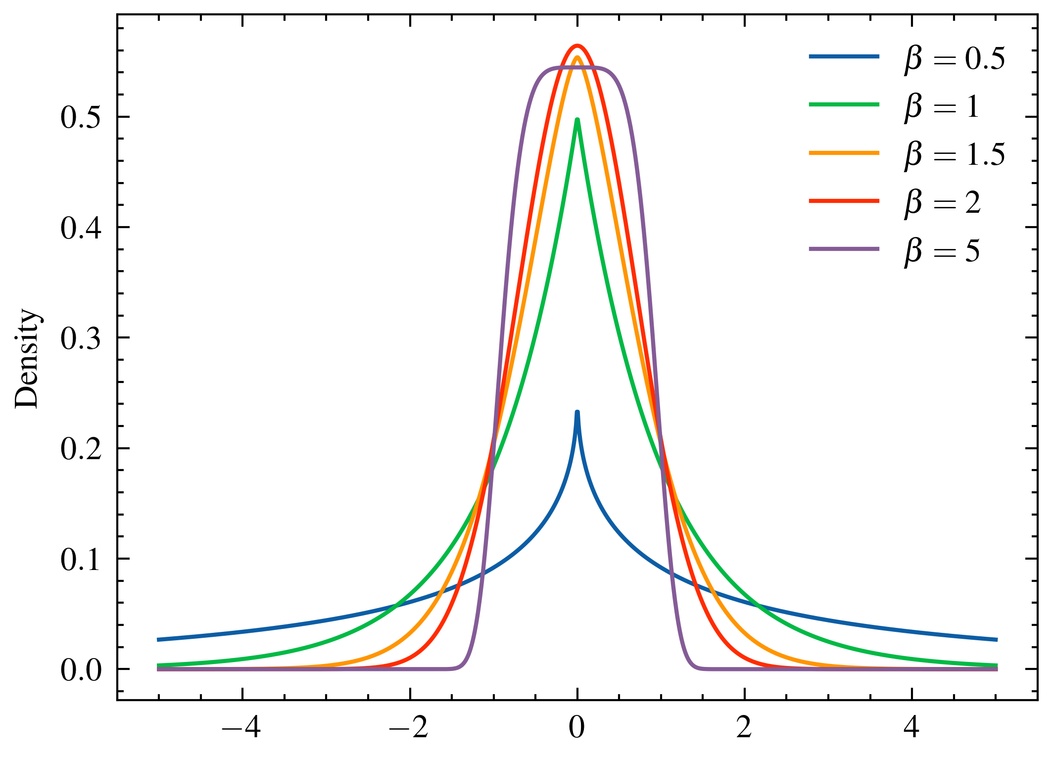
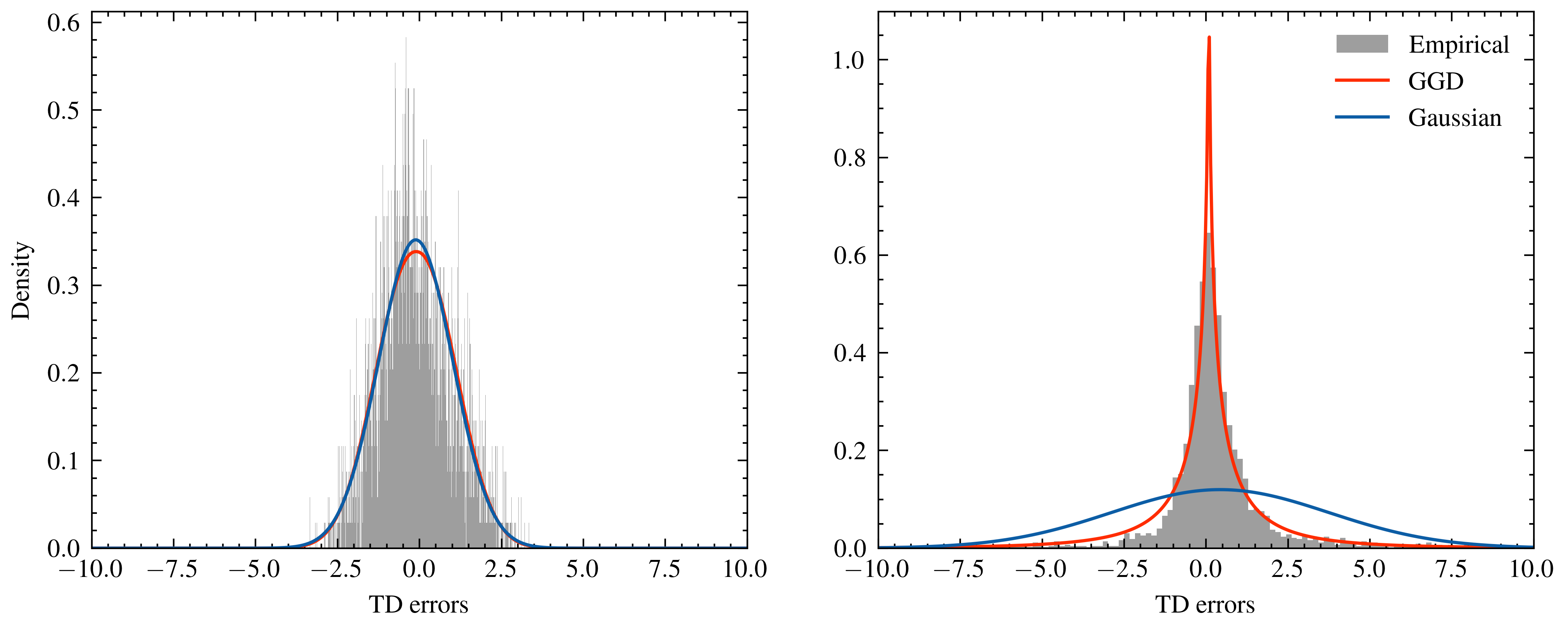
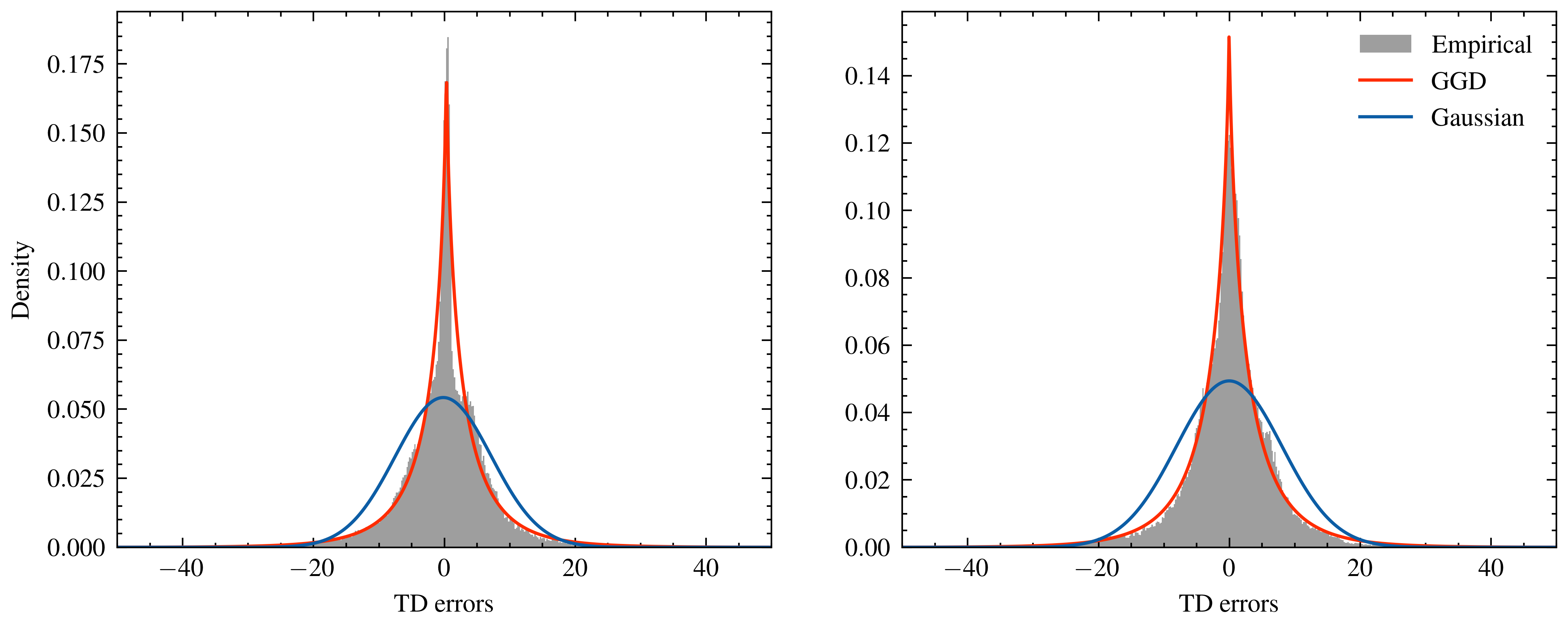
A notable enhancement to the normality hypothesis is the use of the generalized Gaussian distribution (GGD), also known as the generalized error distribution or exponential power distribution. This flexible family of symmetric distributions, as depicted in Figure 1, encompasses a wide range of classical distributions, including Gaussian, Laplacian, and uniform distributions, all adjustable via a shape parameter [5]. This specific parameter allows for fine-tuning the distribution to match the characteristics of TD error distribution, providing a more reliable representation of uncertainty.
Contributions
Our primary contribution is the introduction of a novel framework of generalized Gaussian error modeling in deep RL, enabling robust training methodologies by incorporating the distribution’s shape. This approach addresses both data-dependent noise, i.e., aleatoric uncertainty, and the variance of model estimates, i.e., epistemic uncertainty, ultimately enhancing model stability and performance.
The key contributions of our work are as follows:
-
1.
Empirical investigations (Section 3.1.1): We conduct empirical investigations of TD error distributions, revealing substantial deviations from the Gaussian distribution, particularly in terms of tailedness. These findings underscore the limitations of conventional Gaussian assumptions.
-
2.
Theoretical exploration (Section 3.1.2): Building on empirical insights, we explore the theoretical suitability of modeling TD errors with a GGD. Theorem 1 demonstrates the effectiveness and well-definedness of the proposed method under leptokurtic error distributions, characterized by . Our experimental results suggest that the estimates of mostly converge within this range, aligning with the empirical findings.
-
3.
Aleatoric uncertainty mitigation (Section 3.1): We investigate the implications of the distribution shape on the estimation and mitigation of aleatoric uncertainty. GGD error modeling enables the quantification of aleatoric uncertainty in a closed form, indicating a negative relation to the shape parameter on an exponential scale, with a constant scale parameter . We also leverage the second-order stochastic dominance of GGD to weight error terms proportional to , enhancing the model’s robustness to heteroscedastic aleatoric noise by focusing on less spread-out samples.
-
4.
Epistemic uncertainty mitigation (Section 3.2): We introduce the batch inverse error variance weighting scheme, adapted from the batch inverse variance scheme [38], to account for both variance and kurtosis of the estimation error distribution. This scheme down-weights high-variance samples to prevent noisy data and improves model robustness by focusing on reliable error estimates.
-
5.
Experimental evaluations (Section 4): We conduct extensive experimental evaluations using policy gradient algorithms, demonstrating the consistent efficacy of our method and significant performance enhancements.
2 Background
We consider a Markov decision process (MDP) governed by state transition probability , with and represent the state and action at step , respectively [58]. Within this framework, an agent interacts with the environment via a policy , leading to the acquisition of rewards .
Numerous model-free deep RL algorithms leverage TD updates for value function approximation [21, 26, 42, 43, 52]. In these methods, neural networks parameterized by are trained to approximate the state-action value by minimizing the error between the target and predicted value:
| (1) |
where the target is computed according to Bellman’s equation:
| (2) |
Typically, TD updates involve minimizing the mean squared error (MSE) loss through stochastic gradient descent. This minimization implicitly presumes that errors conform to a Gaussian distribution with zero-mean, consistent with the principles of MLE.
For clarity, we henceforth omit the learnable parameter and adopt subscript notation for function arguments, e.g., .
2.1 Uncertainty
Uncertainty in neural networks is commonly decomposed into two sources: aleatoric and epistemic [13, 14, 31, 63]. Epistemic uncertainty arises from limitations within the neural network and can potentially be reduced through further learning or model improvements. In contrast, aleatoric uncertainty stems from the inherent stochasticity of the environment or the dynamics of the agent-environment interactions and is fundamentally irreducible.
This distinction is crucial in the context of RL, where areas with high epistemic uncertainty need to be explored, whereas exploring areas with high aleatoric uncertainty may lead to ineffective training, since the agent might have adequate knowledge but insufficient information for decisive actions. Quantifying aleatoric uncertainty is known to facilitate learning dynamics of stochastic processes and enables risk-sensitive decision making [10, 54, 65].
To address aleatoric uncertainty, variance networks, denoted by to distinguish them from the value approximation head , are frequently employed [3, 31, 33, 38, 40, 47]. The estimated variance from is utilized for heteroscedastic Gaussian error modeling, with , thereby quantifying aleatoric uncertainty [54]. This network is trained by maximizing the log likelihood function of the Gaussian distribution or minimizing the Gaussian negative log likelihood (NLL) loss. The variance of estimated values is also used for batch inverse variance (BIV) weighting in inverse-variance RL [38]. This regularization effectively captures epistemic uncertainty with a regularizing temperature :
| (3) | ||||
where the BIV weight with empirical variance , and is either a hyperparameter or numerically computed to ensure a sufficient effective batch size. In the official implementation, the sample variance with Bessel’s correction is used as a variance estimator, which is particularly apparent given a small sample size, i.e., an ensemble number of five.
2.2 Tailedness
While mainstream machine learning literature often prioritizes on capturing central tendencies, the significance of extreme events residing in the tails for enhancing performance and gaining a deeper understanding of learning dynamics cannot be overlooked. This is especially relevant for MLE base on the normality assumption, which is commonly applied in variance network frameworks. Focusing solely on averages or even deviations is proven to be inadequate in the presence of outlier samples [11, 23].
For instance, consider the impact of non-normal samples on the estimate of the variance, as described in 1 with proof presented in Section B.1.
Proposition 1 (Biased variance estimator [68]).
Let be a sequence of independent, non-normally distributed random variables from a population with mean , variance , and kurtosis . Then, with the MLE estimators under normality assumption, i.e., for mean and for variance, the variance estimator exhibits bias. Specifically, it will be negatively biased when and positively biased when .
1 elucidates that the standard error of estimated TD error variance is a function of kurtosis . With heavy-tail distributions, the standard error of variance estimates, through networks trained by Gaussian NLL [47, 3], may also be underestimated, highlighting the influence of kurtosis on variance estimation. Furthermore, it is shown that the likelihood ratio statistics for variance estimator depends on kurtosis even for large [68]. This emphasizes the necessity of accounting for tailedness to derive robust variance estimates confidently.
Remark 1 (Varietal variance estimator [6]).
The dependence of the standard error of the variance estimator on kurtosis impacts both the bias and variance of variance estimation. Specifically, when the kurtosis of the underlying distribution exceeds zero, assuming normality tends to result in an underestimation of the confidence interval of variance estimation.
Gumbel error modeling
Recent applications of Gumbel distribution closely related to TD learning have emerged for estimating the maximum value in the Bellman update process [22, 28]. These approaches capitalize on the foundation of the extreme value theorem, which states that maximal values drawn from any exponential-tailed distribution follow the Gumbel distribution [19, 44]. Compared to conventional distributional RL algorithms employing Gaussian mixture or quantile regression [10, 55], this approach showcases superior control performance. However, it has been observed that while Gumbel modeling initially aligns with the error distribution propagated through the chain of operations, its Gumbel-like attribute may diminish over the course of training [22]. We instead propose a novel approach utilizing GGD, which offers flexibility in expressing the tail behavior of diverse distributions. This method is adaptable to wider range of MDPs, even those without operators.
3 Methods
Our approach introduces enhancements to the loss function derived from (3), incorporateing tailedness into both loss attenuation and regularization terms:
| (4) | ||||
where and represent the alpha and beta networks, respectively. Here, , and . These dual loss terms effectively capture aleatoric and epistemic uncertainties, respectively. The subsequent subsections provide a detailed rationale for this modification.
3.1 Generalized Gaussian error modeling
One simple yet promising approach to address non-normal heteroscedastic error distributions involves modeling the per-error distribution using a zero-mean symmetric GGD [9, 24, 61, 69]:
| (5) |
where and represent the scale and shape parameter, respectively. This method not only allows for modeling each non-identical error by parameterizing the GGD with different and at step , but also offers a flexible parametric form that adapts across a spectrum of classical distributions from Gaussian to uniform as increases to infinity [16, 25, 46, 48].
The shape parameter serves as a crucial structure characteristic, distinguishing underlying mechanisms. The kurtosis , commonly used to discern different distribution shapes, is solely a function of and is defined as Pearson’s kurtosis minus three to emphasize the difference from Gaussian distribution [12]:
| (6) |
This implies that distributions with are leptokurtic, i.e., , indicating a higher frequency of outlier errors compared to the normal error distribution. With only one additional parameter to characterize the distribution, GGD effectively expresses differences in tail behavior, a capability distributions dependent solely on location or scale parameters lack.
Remark 2.
Despite the GGD having three parameters, we only employ the estimation for GGD error modeling to minimize computational overhead, setting the scale parameter to one. While this may slightly limit the expressivity of the error model, it significantly enhances training stability. The impact of omitting the parameter is minimal, as moments influenced by can also be represented by . Additionally, this simplification offers implementation advantages, requiring only a slight change in the loss function to migrate from variance networks, i.e., from Gaussian to GGD NLL.
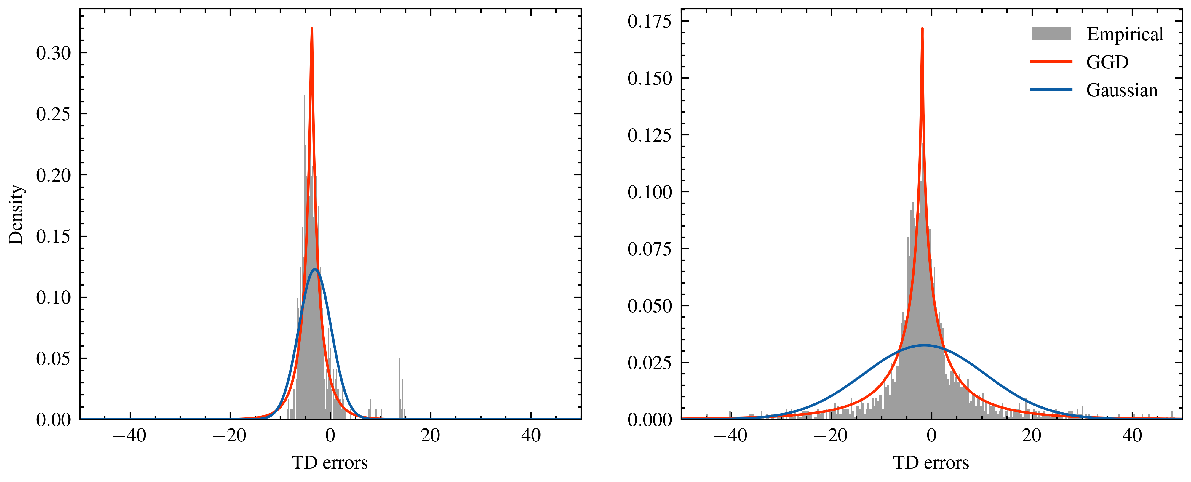
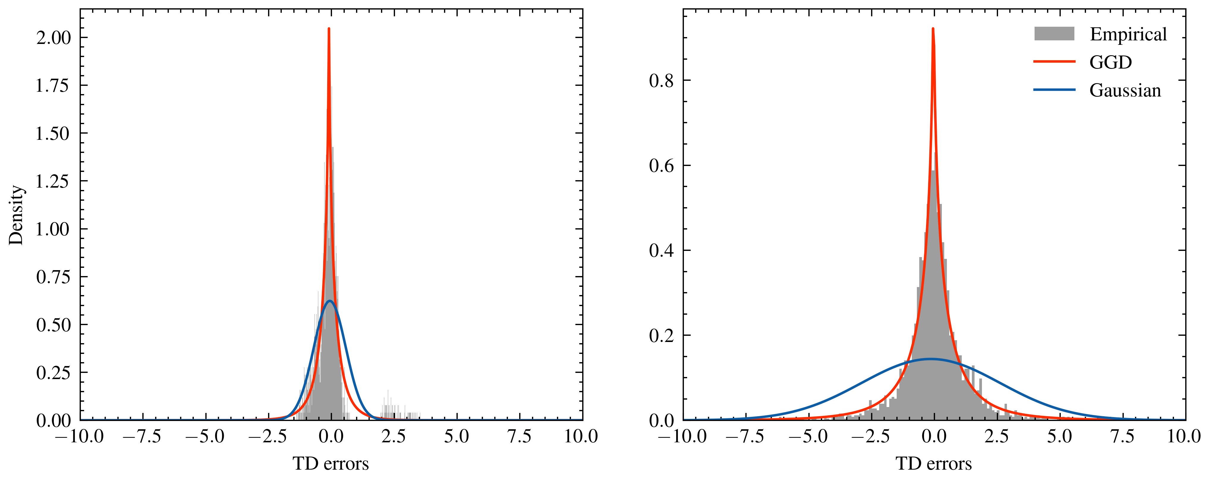
3.1.1 Empirical evidence
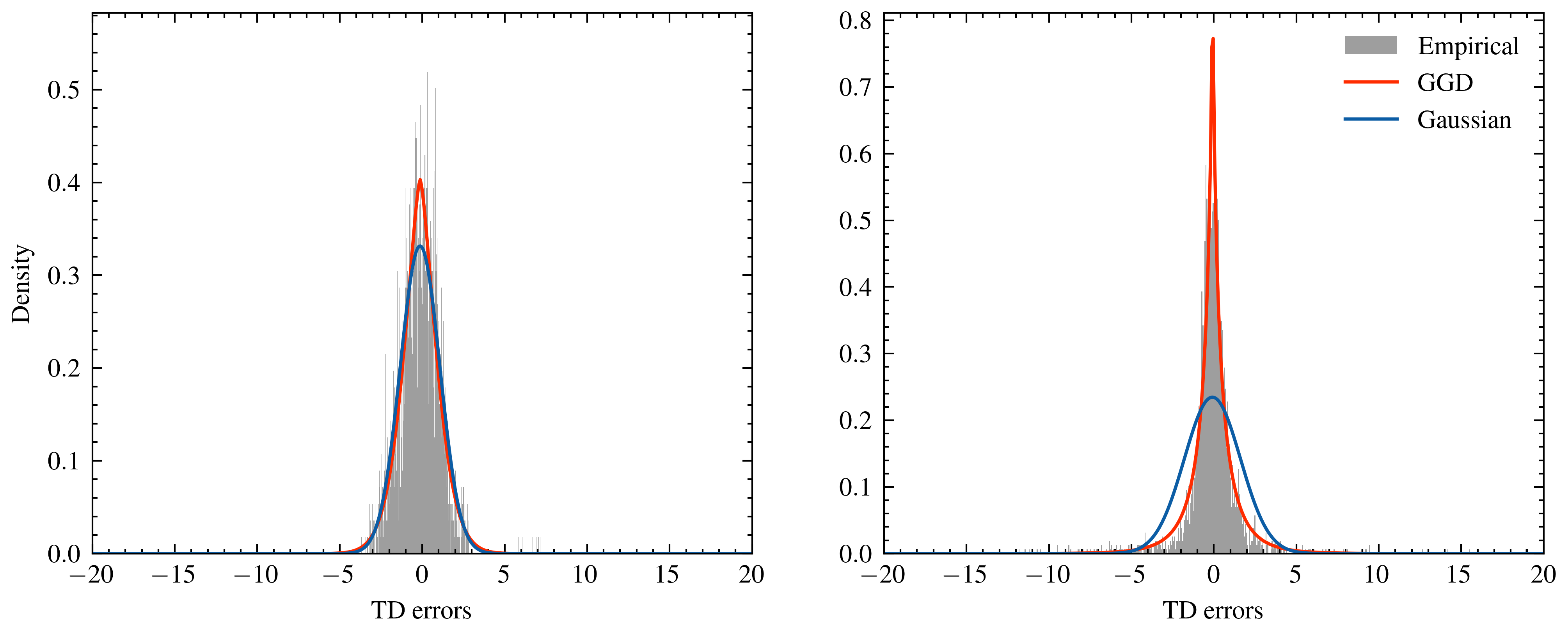
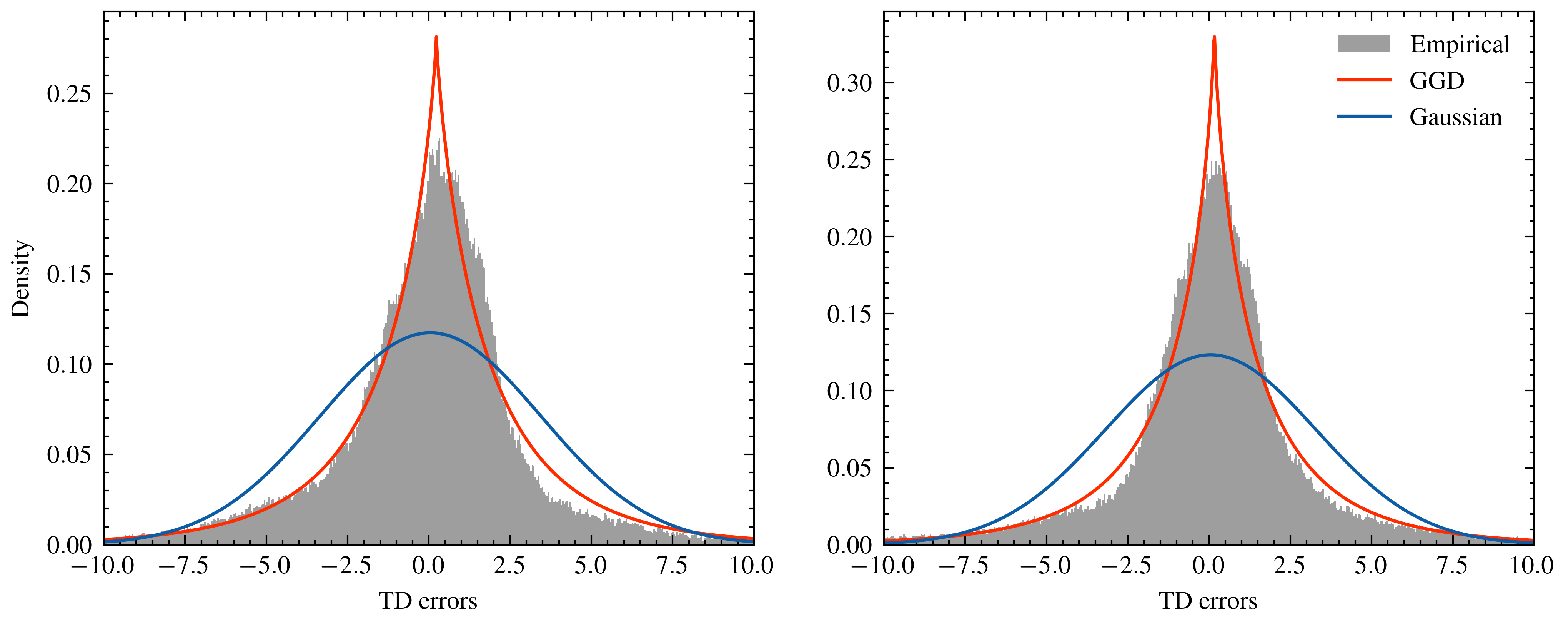
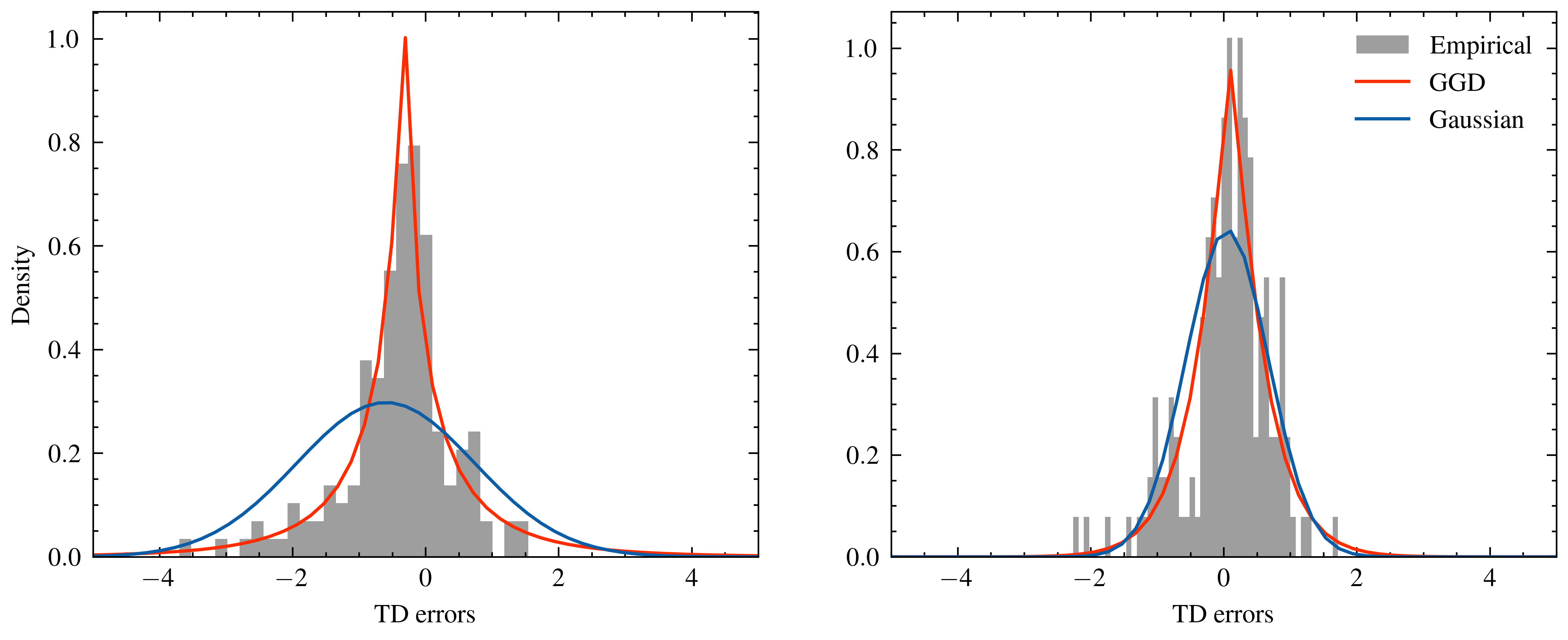
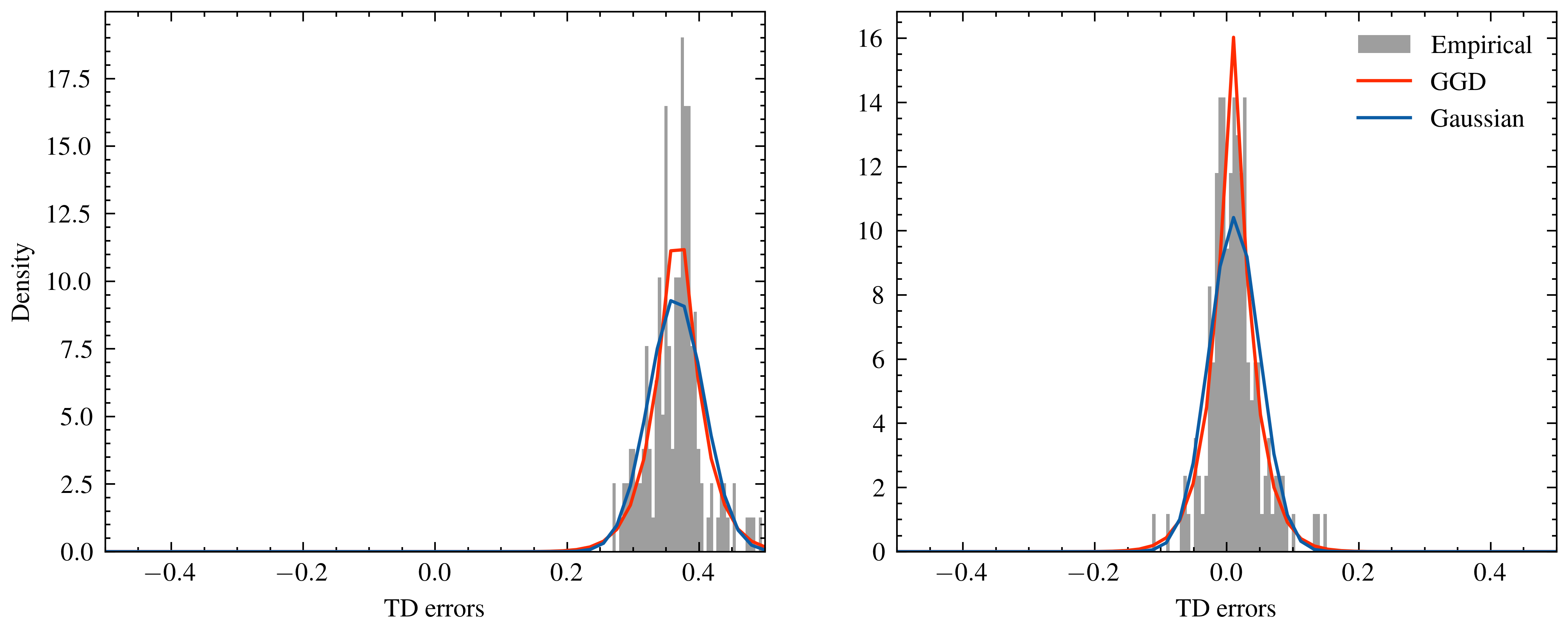
Figure 2 presents empirical findings that reveal a departure from Gaussian distribution in TD errors, evidenced by well-fitted GGDs and pronounced differences in the shape of distributions. This non-normality is particularly notable when contrasting initial and final evaluations, suggesting an escalating significance of tailedness throughout the training process. We hypothesize that such divergence from normality stems from the exploratory nature of agent behavior. During exploration, agents often encounter unexpected states and rewards, leading to a broader spectrum of TD errors than those seen in purely exploitative scenarios. Consequently, increased variability contributes to the emergence of non-normal distributions, notably with heavier tails.
Furthermore, the observed evolution in TD error tails underscores the shifting interplay between aleatoric and epistemic uncertainties. As training progresses, the influence of aleatoric errors increases as epistemic uncertainty diminishes, potentially resulting in non-normally distributed errors with heavier tails.
3.1.2 Theoretical analysis
Given the empirical suitability of GGD for modeling TD errors, we conduct an in-depth theoretical examination of GGD. We begin by demonstrating the well-definedness of GGD regression, with a specific emphasis on the positive-definiteness of its PDF under certain conditions.
This theorem guarantees the well-definedness of the NLL of the GGD. It ensures that the PDF is guaranteed to be positive everywhere under highly probable conditions of , thus affirming the suitability of the NLL as a loss function for a valid probability distribution. In fact, it is known that parameter estimation for GGD can also be numerically accomplished by minimizing the NLL function, with asymptotic normality, consistency, and efficiency of the estimates ensured under suitable regularity conditions [1]. This positive-definiteness not only implies a theoretical property but also has practical implications in deep RL, where ensuring stability and convergence is crucial. The positive-definiteness of the PDF of GGD shown in the proof, elaborated in Section B.2, also assures that the function integrates to one.
The shape parameter also introduces a desirable property of risk-aversion to GGD, which can be mathematically formulated by stochastic dominance [34, 39]. Stochastic dominance, a concept assessing random variables via a stochastic order, reflects the shared preferences of rational decision-makers.
Theorem 2 (Second-order stochastic dominance [16]).
Consider two random variables and , where and . If , then exhibits second-order stochastic dominance over . This dominance implies, for all ,
| (7) |
where denotes the cumulative distribution function.
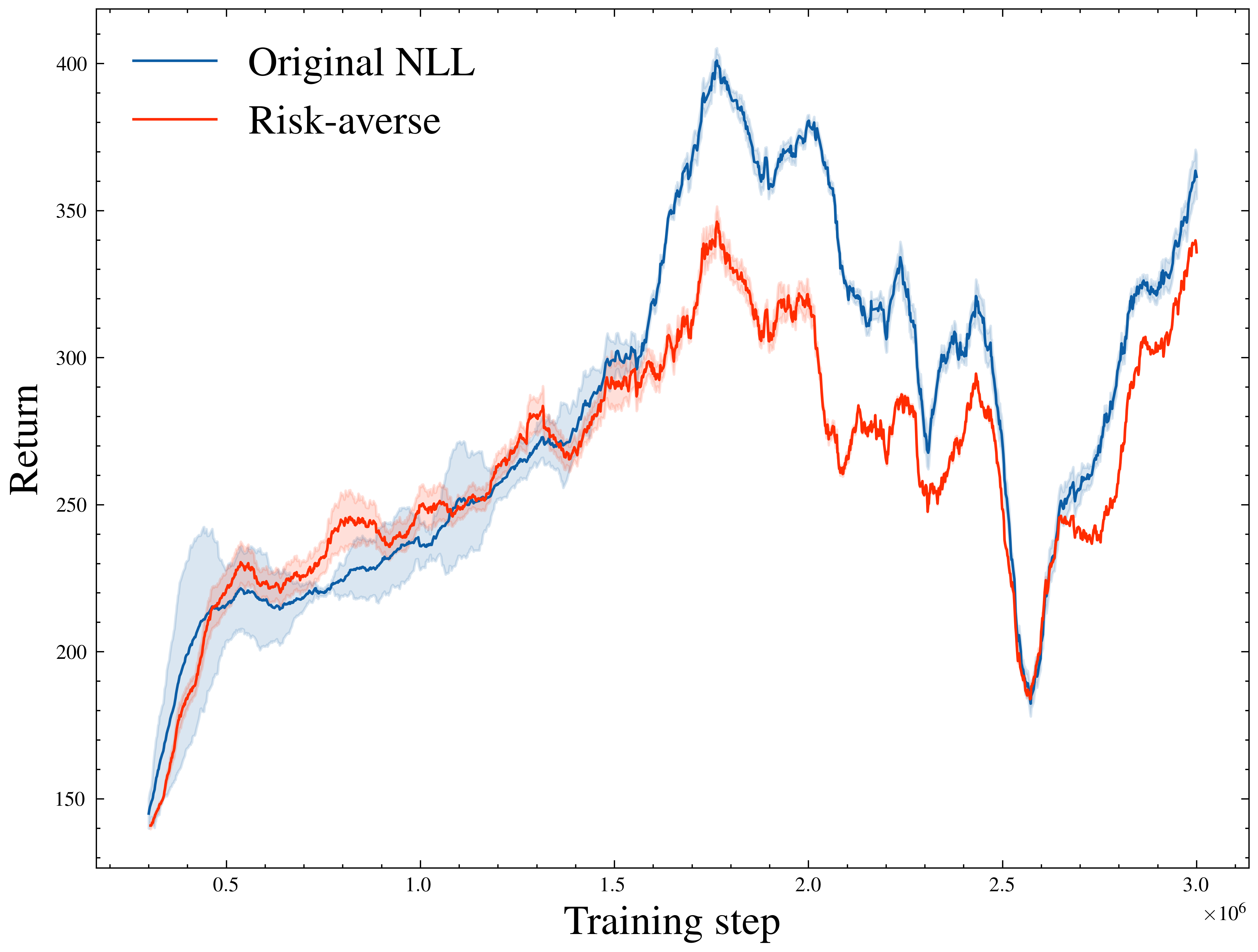
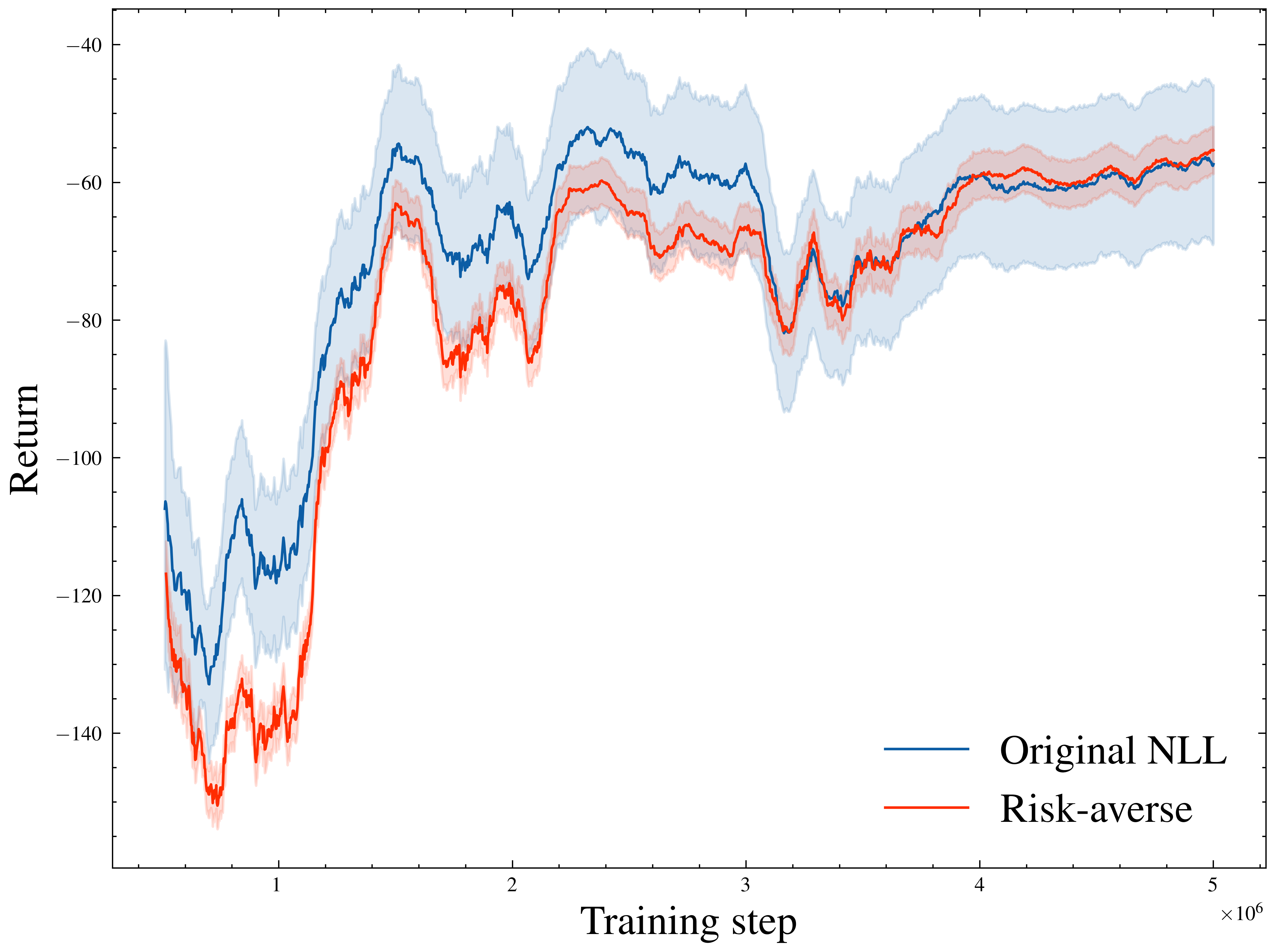
The above theorem, with its proof detailed in Section B.3, suggests second-order stochastic dominance of TD errors. This dominance signifies a preference for risk-aversion, wherein the dominant variable exhibits greater predictability and maintains expectations that are equal to or higher than those of for all concave and non-decreasing functions [49]. Formally, for such a function , we have , with denoting expectation.
The dominance relationship among GGD random variables, determined by the shape parameter , reinforces the suitability of GGD for modeling errors in TD learning. Leveraging this risk-aversion, the application of the risk-averse weighting in capitalizes on the tendency of GGD to learn from relatively less spread-out samples, thereby enhancing robustness to heteroscedastic noise.
Remark 3.
The training of the critic is more directly influenced by aleatoric uncertainty, since only the critic loss is a direct function of the state, action, and reward, with the actor being downstream of the critic in uncertainty propagation. GGD error modeling enables us to quantify aleatoric uncertainty as a closed form, i.e., [61]. Remarkably, aleatoric uncertainty exhibits a negative proportionality to the shape parameter on an exponential scale, with a constant scale parameter adopted in our implementation employing a beta head exclusively. Building on this, risk-averse weighting mitigates the negative impacts of noisy supervision by assigning higher weights to errors with lower aleatoric uncertainty for the loss attenuation term.
3.2 Batch inverse error variance regularization
When estimating the uncertainty of target estimates, as employed in BIV weighting, potential bias can arise [29, 35]. Conversely, the bias of TD errors remains notably small with the assumption of constant value approximation bias [20]. Motivated by this, we propose the batch inverse error variance (BIEV) weighting:
| (8) |
incorporating the concept of error variance explicitly into BIV weighting.
Recent investigations have explored advancements in variance estimation, particularly through a constant multiplier, i.e., [32, 67], where denotes sample variance, the MLE estimator of variance. Although non-standard weights may introduce bias in variance estimation, the estimation of inverse variance remains biased due to Jensen’s inequality, even with the use of the unbiased estimator [66]. Consequently, our focus shifts to relative efficiency (RE), where we derive the MSE-best biased estimator (MBBE) in 2.
Proposition 2 (MBBE of variance [53, 67]).
Let be the adjusted variance estimator, with the sample variance and the weight being a function of the sample size and the population kurtosis . Then, the estimator with the least MSE is given by:
| (9) |
Additionally, MBBE of variance has consistent superior efficiency over the sample variance , i.e.:
| (10) |
The reciprocal relationship between sample size and the impact of kurtosis on variance estimation is intuitive, especially for small samples where kurtosis is much more significant. Consequently, we advocate for the adoption of the MBBE in epistemic uncertainty estimation. It’s worth noting that while the derivation of improved estimators presupposes known kurtosis, our method differs by utilizing estimated kurtosis.
As BIV weighting, the BIEV weighting plays a crucial role in enhancing the robustness and efficiency TD updates. By normalizing the weight of each sample in a batch relative to the scale of its epistemic uncertainty compared to other samples, BIEV weighting ensures that the model appropriately accounts for the reliability of the estimate from each data point, resulting in robustness against inaccuracies in variance estimate calibration.
4 Experiments
We conduct a comprehensive evaluation of our proposed method across well-established benchmarks, including MuJoCo [59], and discrete control environments from Gymnasium [60]. Notably, we augment the discrete control environments through the introduction of supplementary uniform action noise to enhance environmental fidelity.
To underscore the versatility and robustness of our approach, we deliberately choose baseline algorithms that cover a wide spectrum of RL paradigms. Specifically, we employ soft actor-critic (SAC) [26], an off-policy -based policy gradient algorithm, and proximal policy optimization (PPO) [52], an on-policy -based method. We focus on adversaries limited to variance networks due to the use of separate target networks in previously mentioned Gumbel error modeling methods. This constraint is intended to focus on computationally efficient algorithms that only incorporate an additional layer, referred to as a head.
The algorithms are implemented using PyTorch [50], within the Stable-Baselines3 framework [51]. We use default configurations from Stable-Baselines3, with adaptations limited to newly introduced hyperparameters. For both PPO and SAC, along with their variants, we employ five ensembled critics. The parameter from (4) is computed with a minimum batch size of 16, and the regularizing temperature is set to . Additional experimental details are provided in Appendix C.
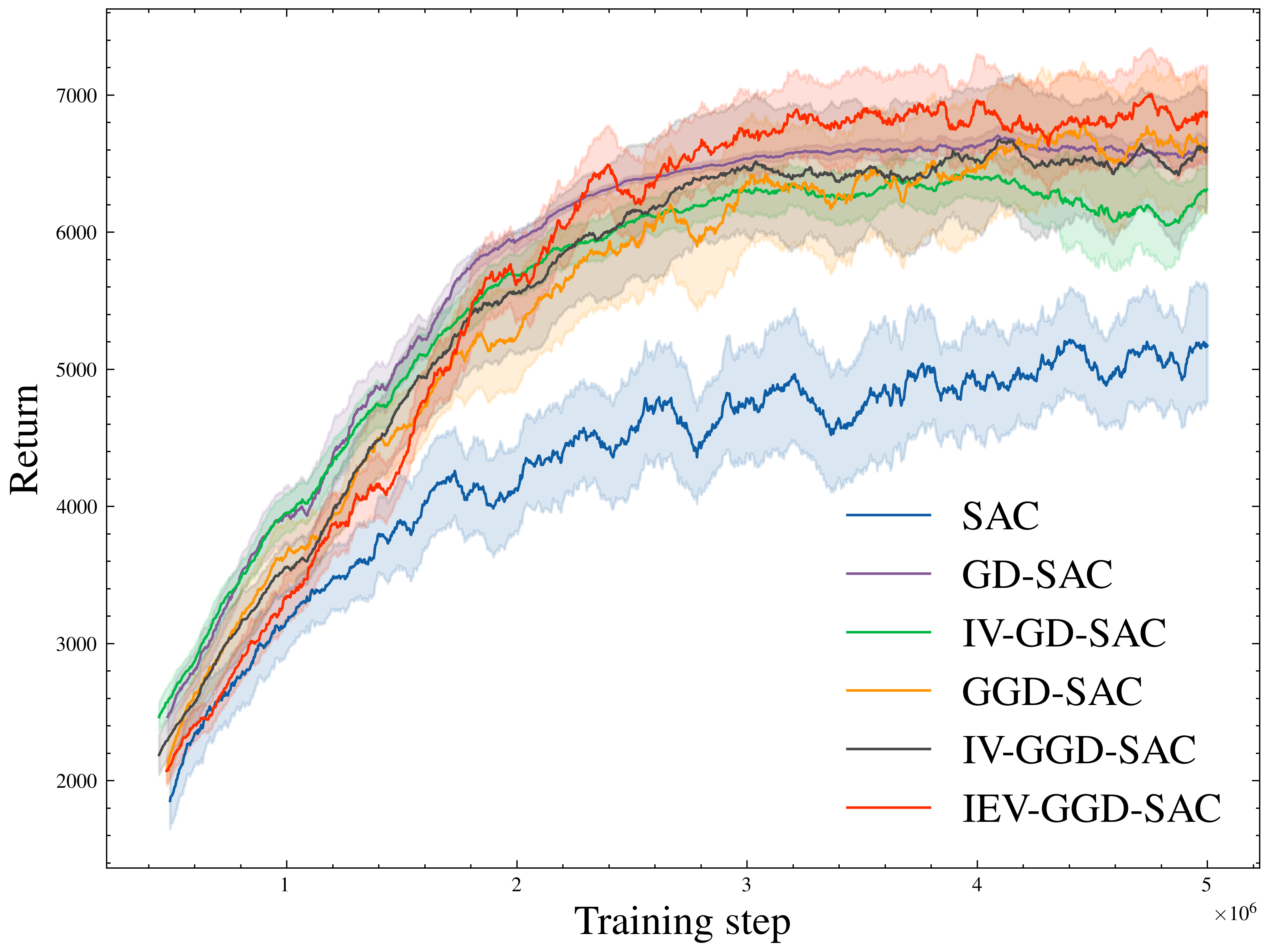
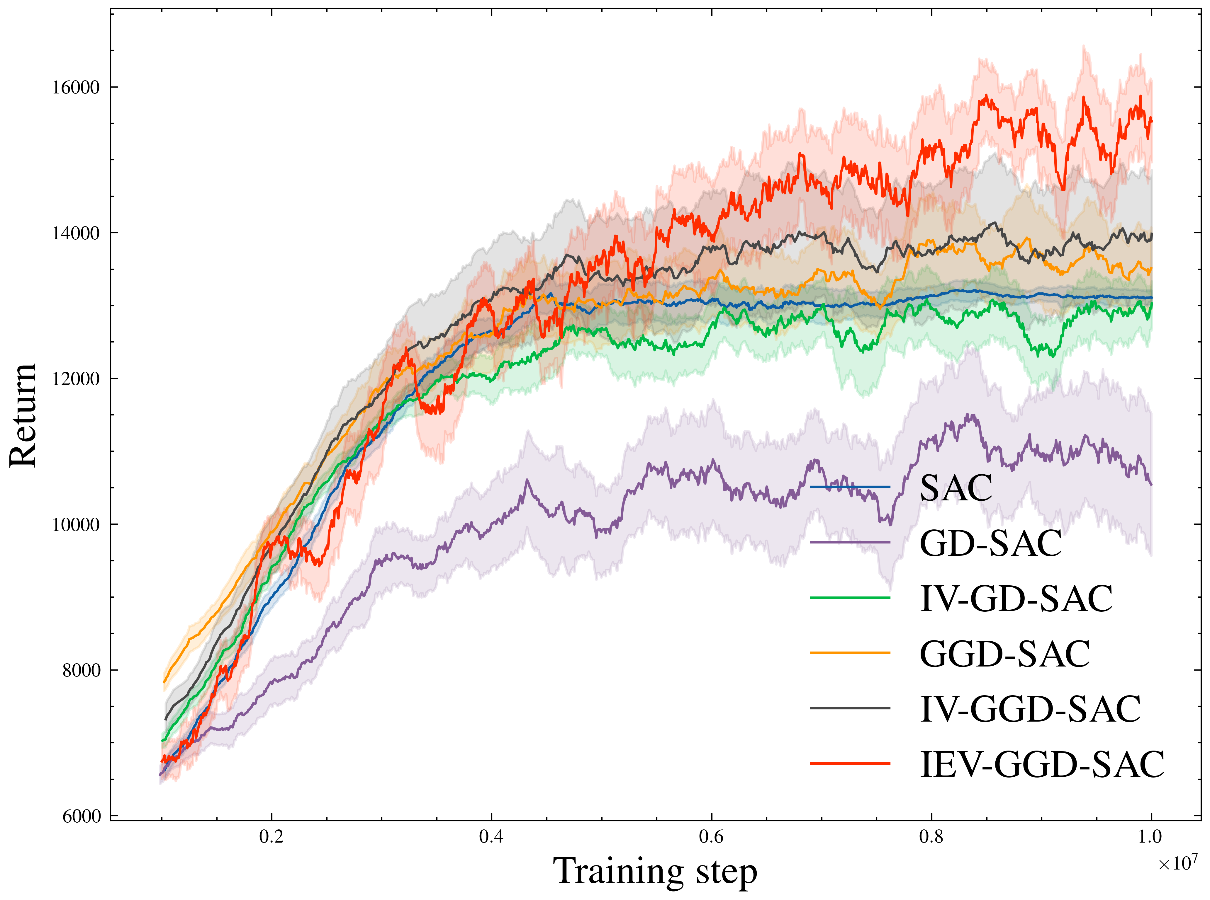
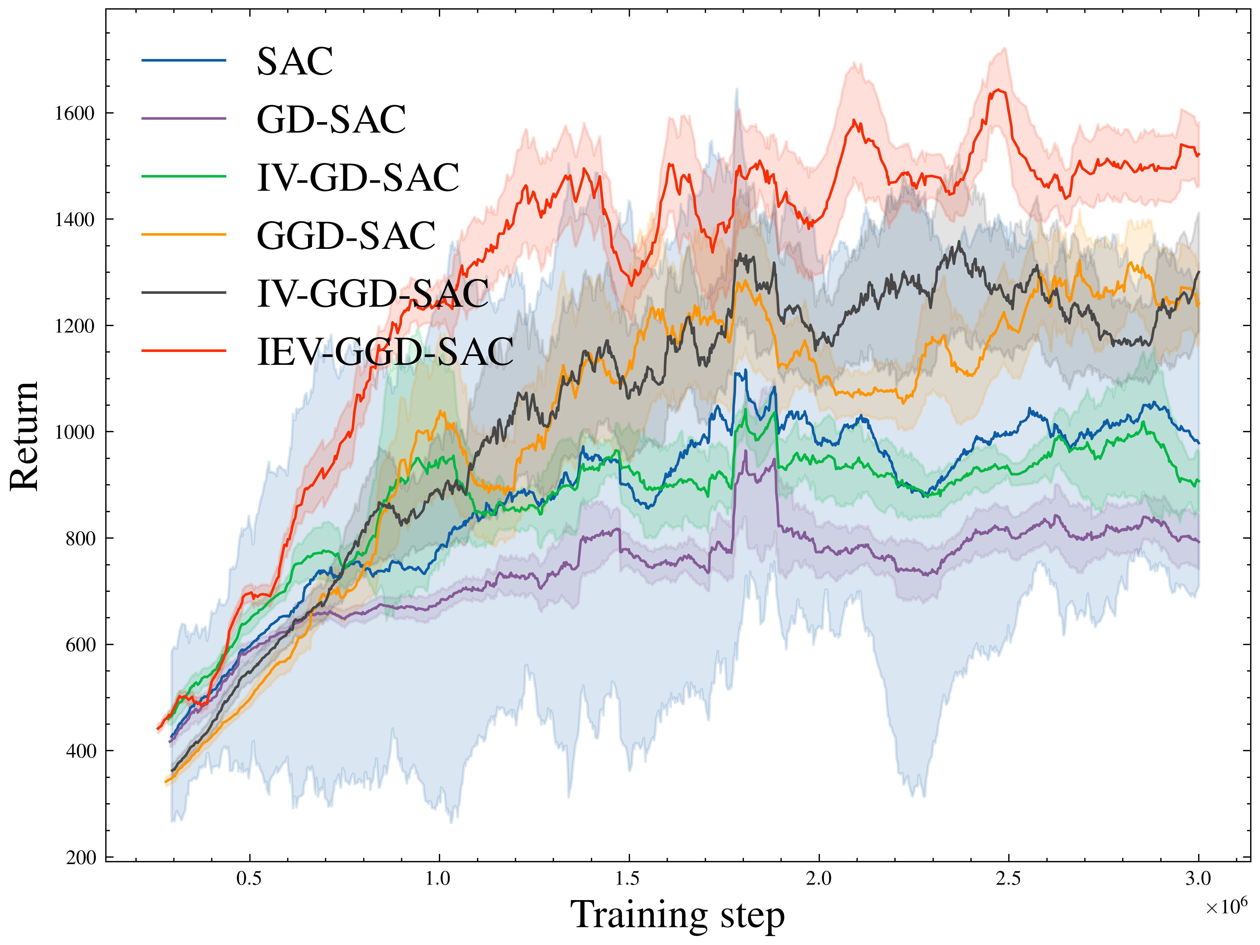
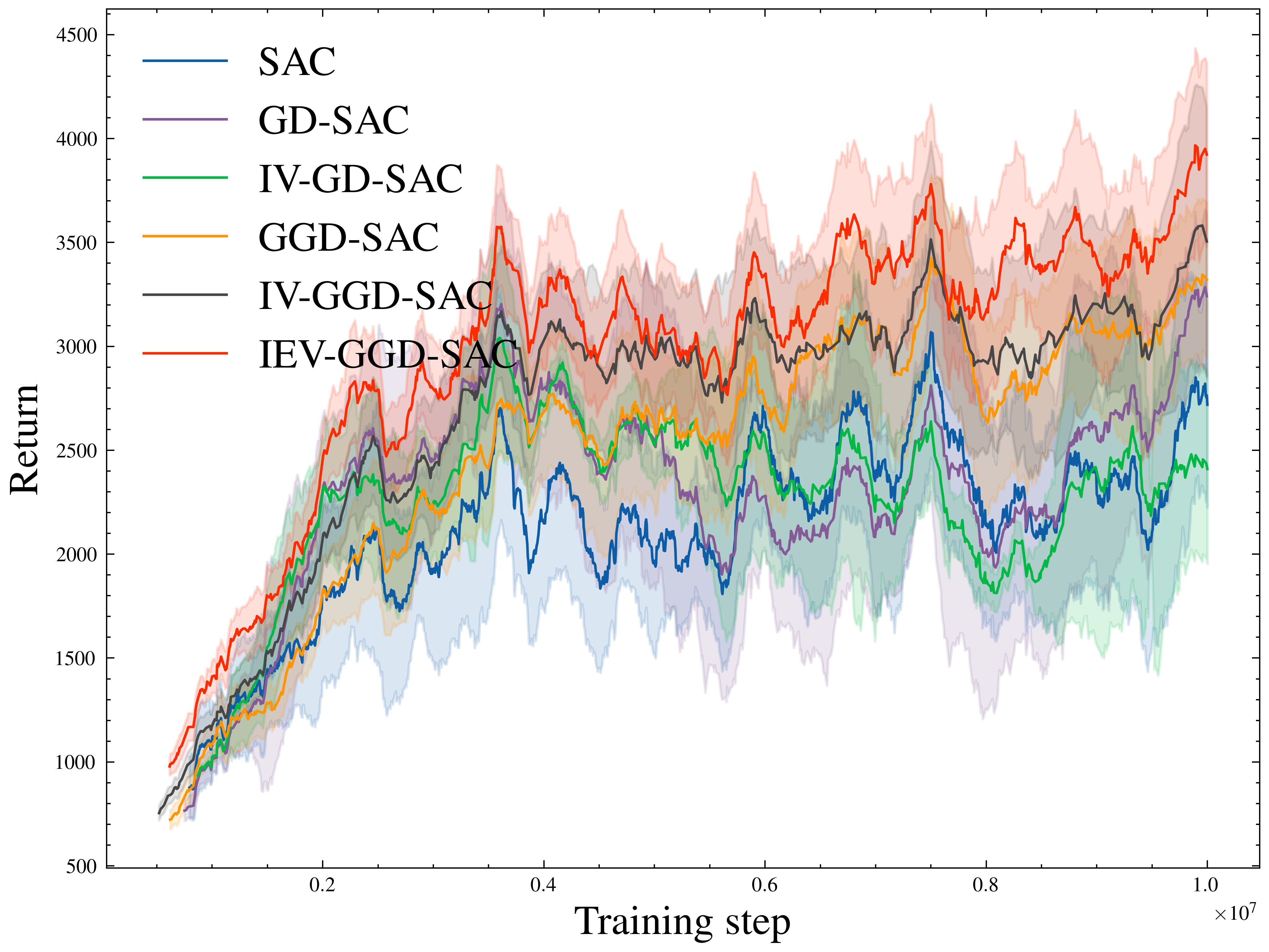
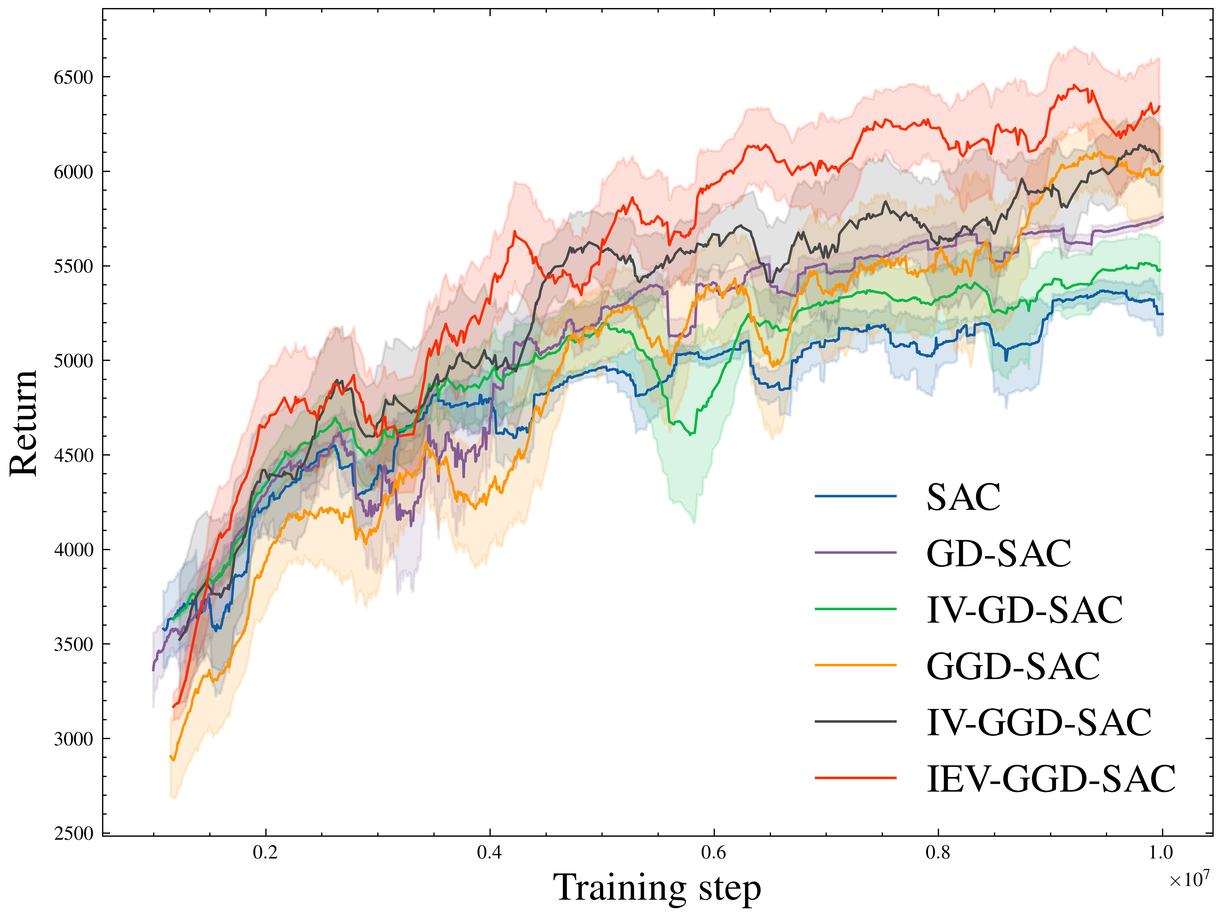
The performance of SAC across different MuJoCo environments is presented in Figure 3. While the variance head degrades performance in certain scenarios, SAC variants employing the beta head consistently lead to better sample efficiency and asymptotic performance. Notable improvements are observed in the HalfCheetah-v4 and Hopper-v4 environments, where the variance head substantially reduces sample efficiency. This suggests that the TD error distributions in these environments may exhibit heavy tails. The impact of BIEV regularization varies by environment but generally performs at least as well as BIV regularization.
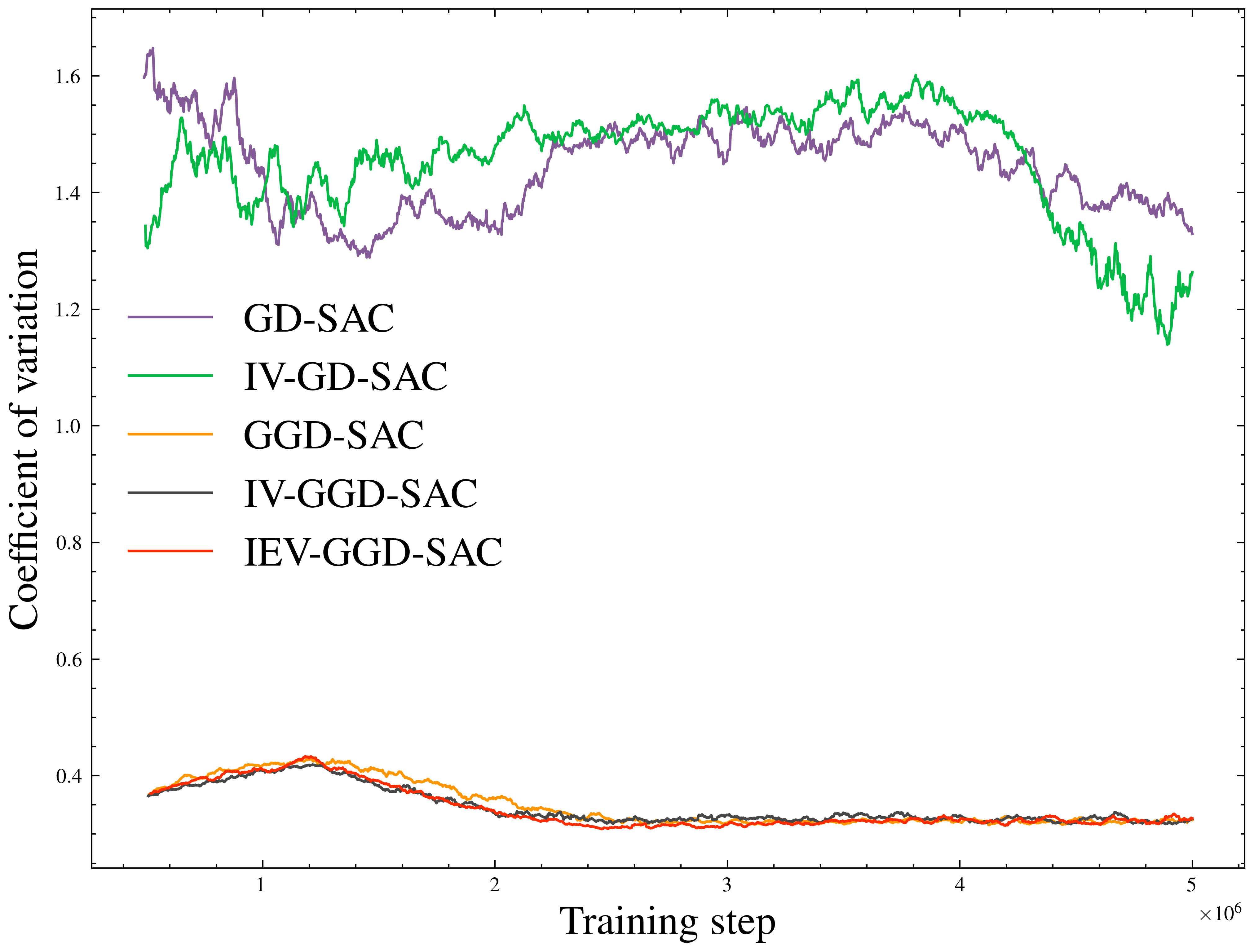
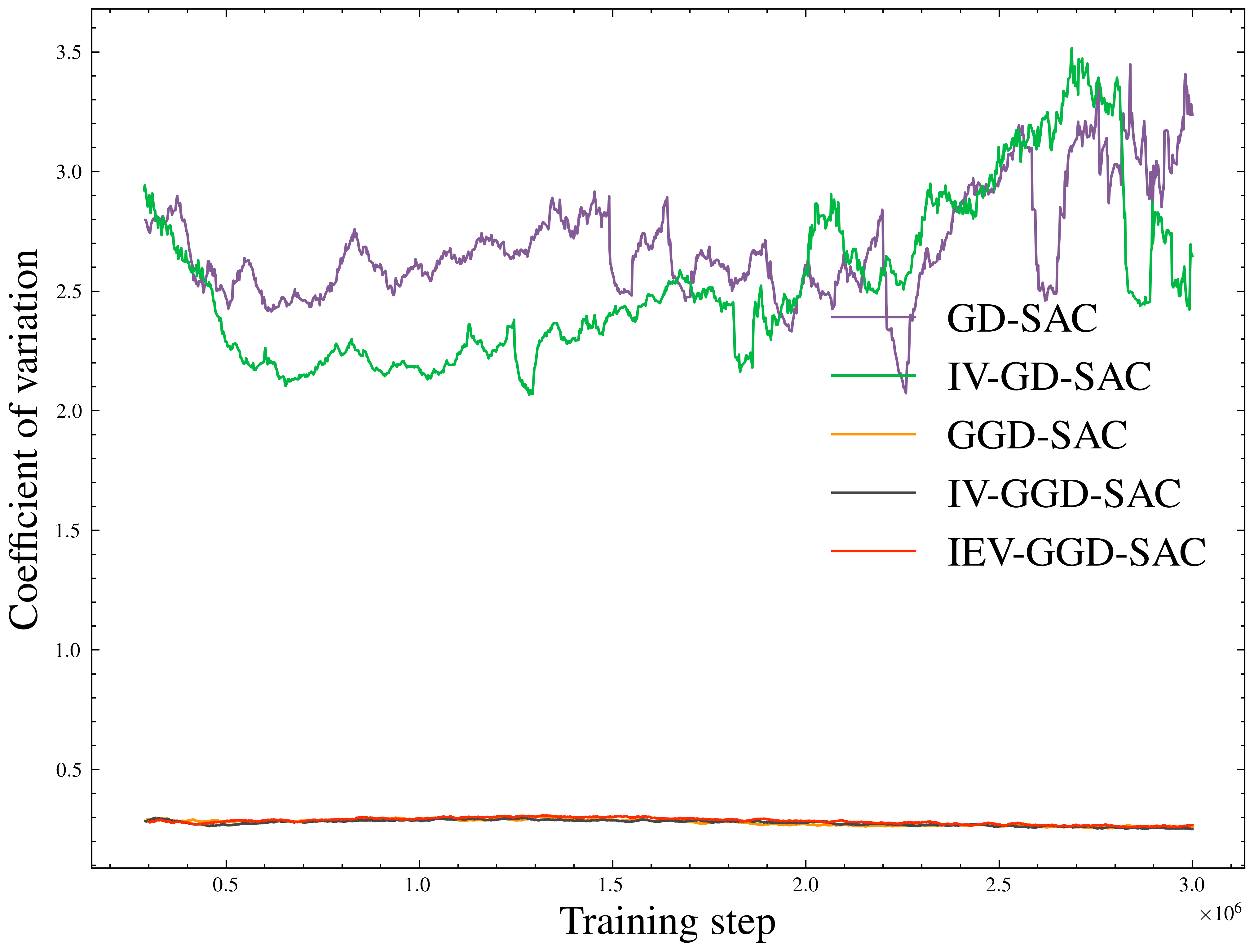
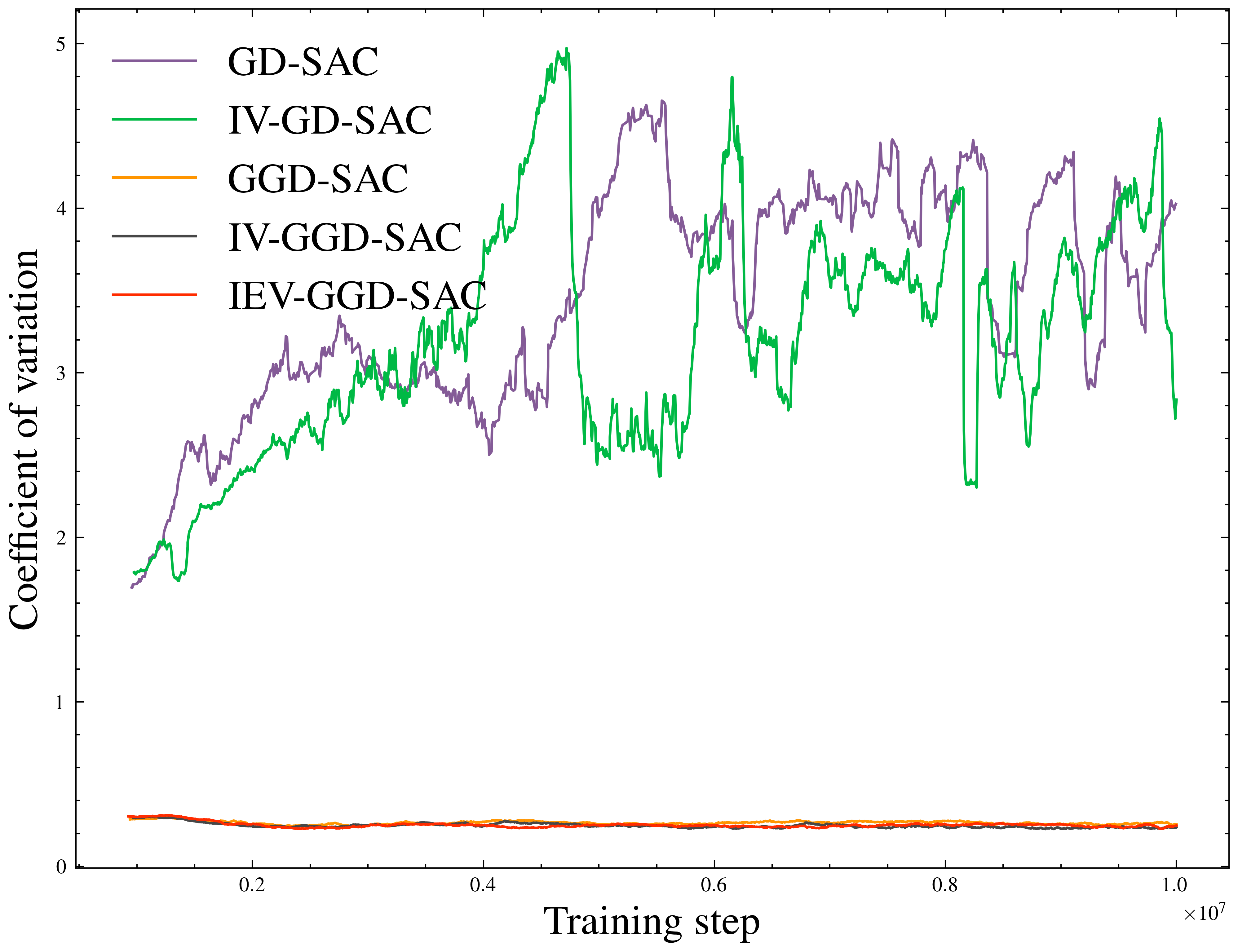
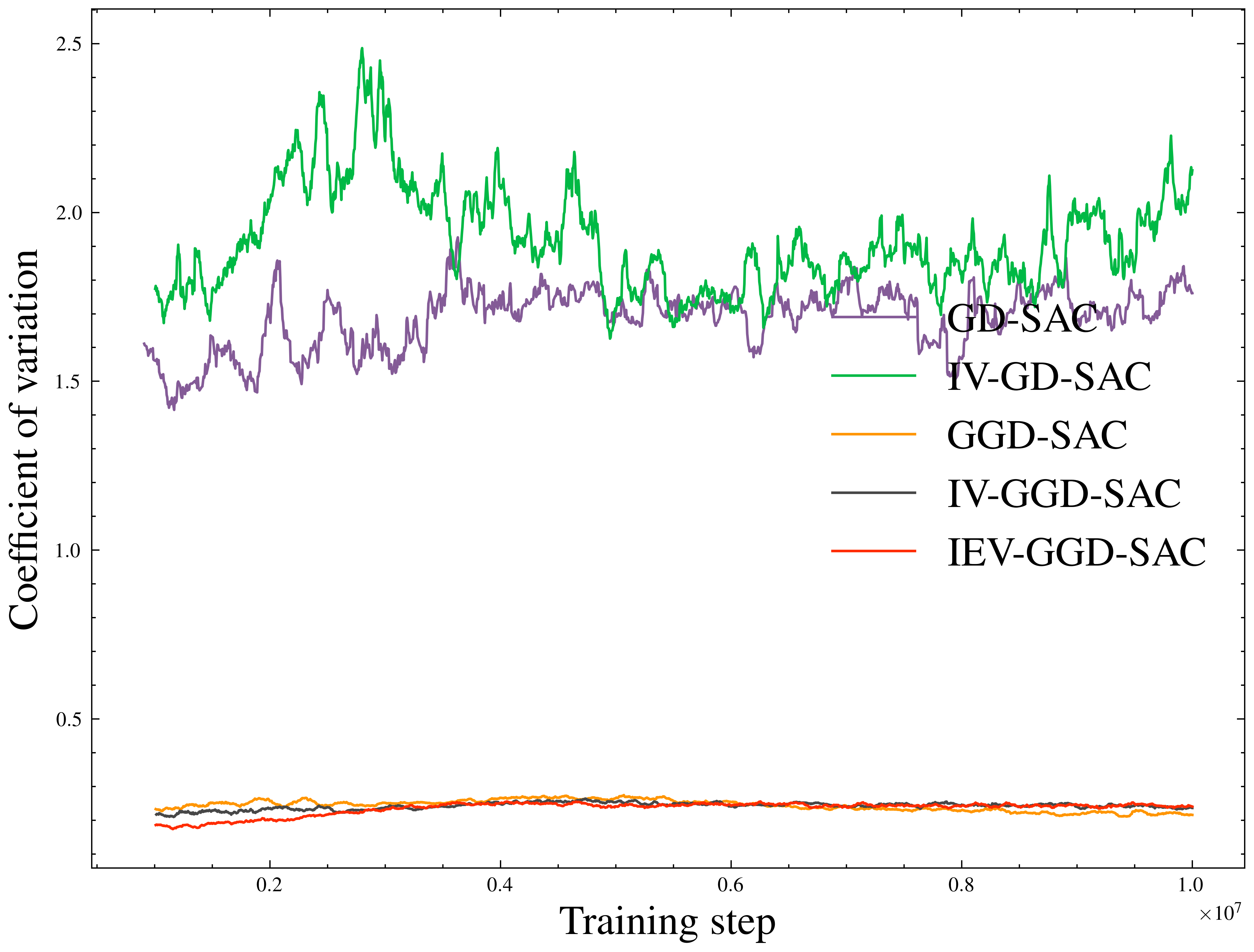
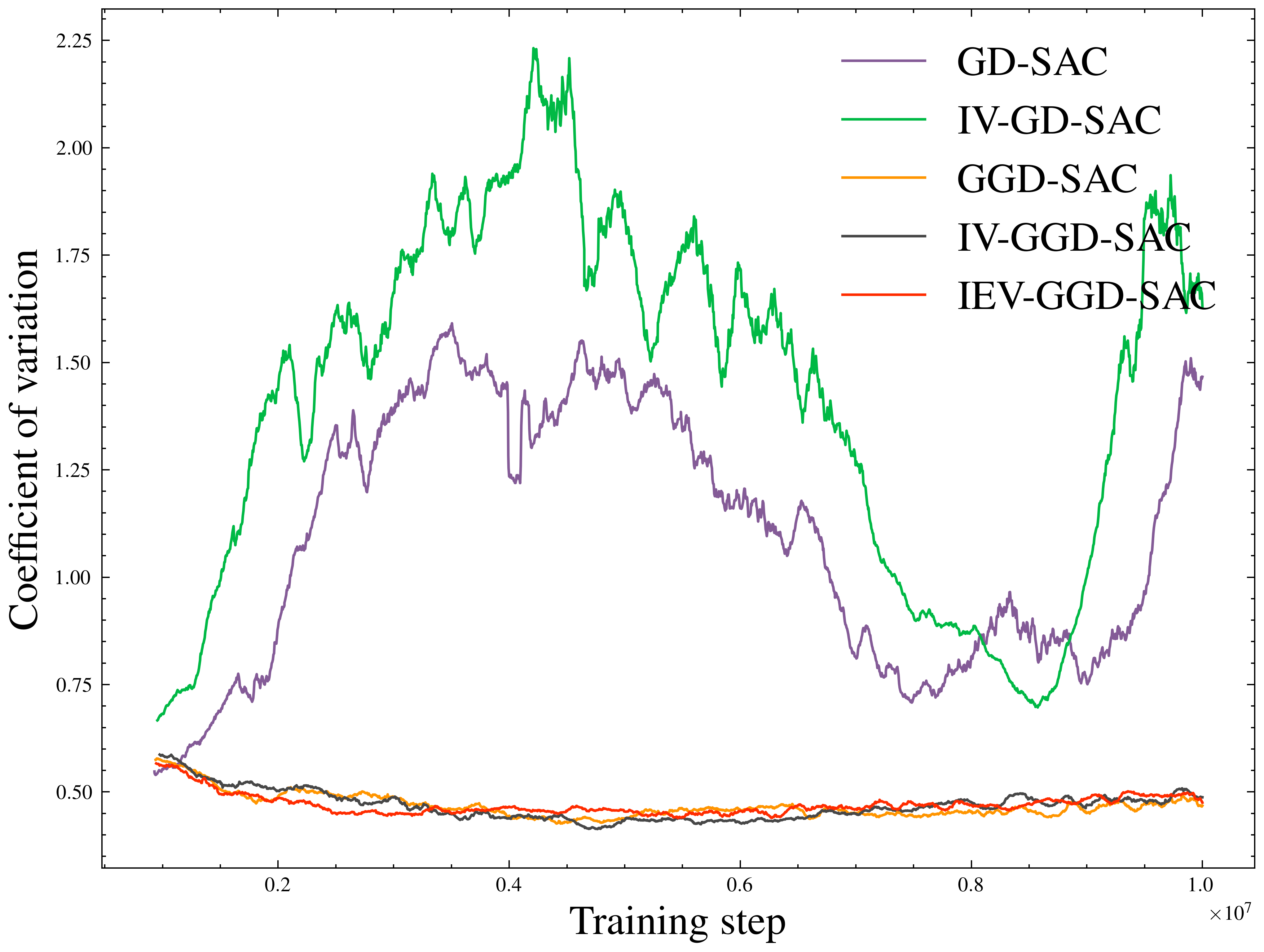
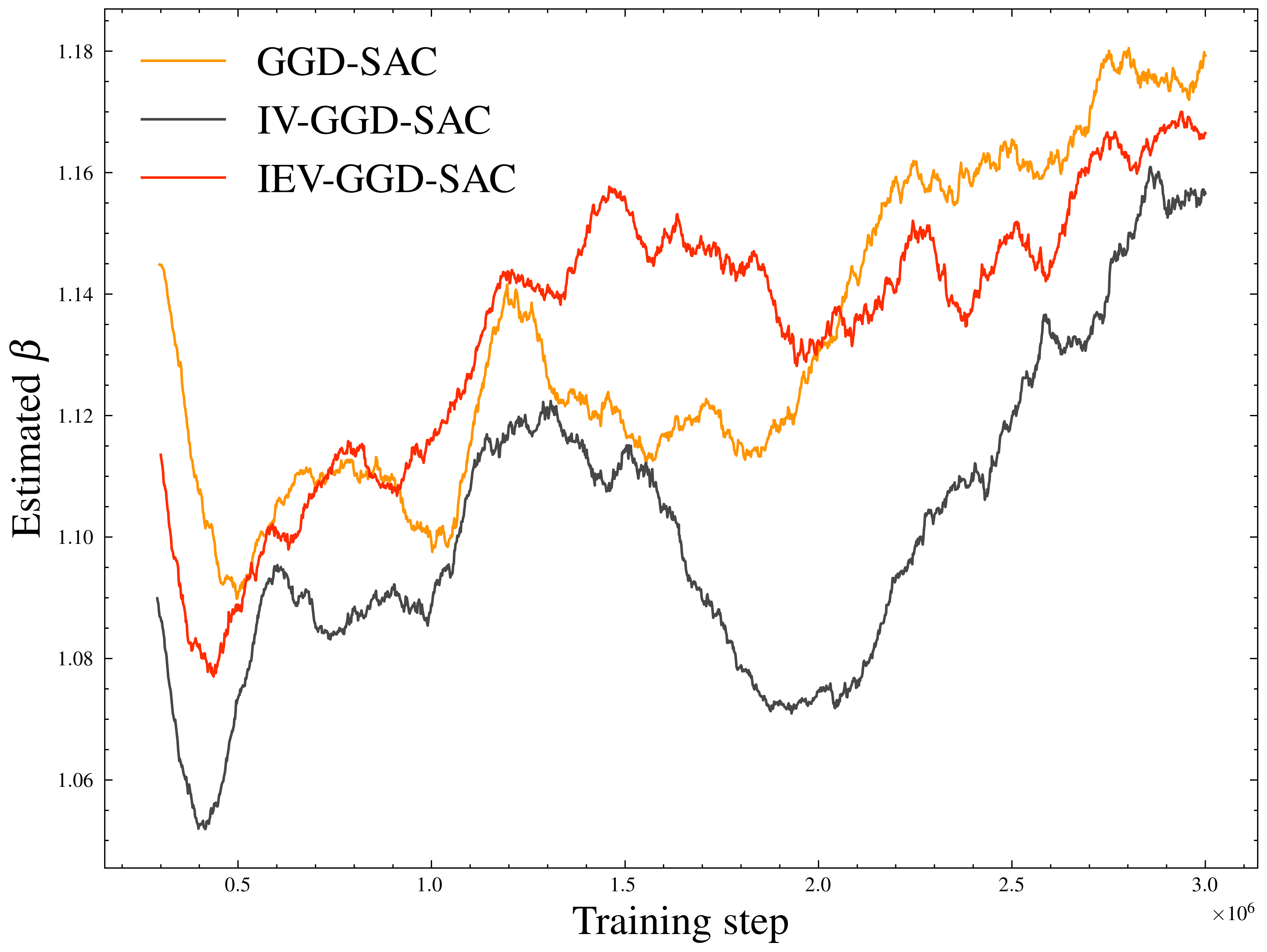
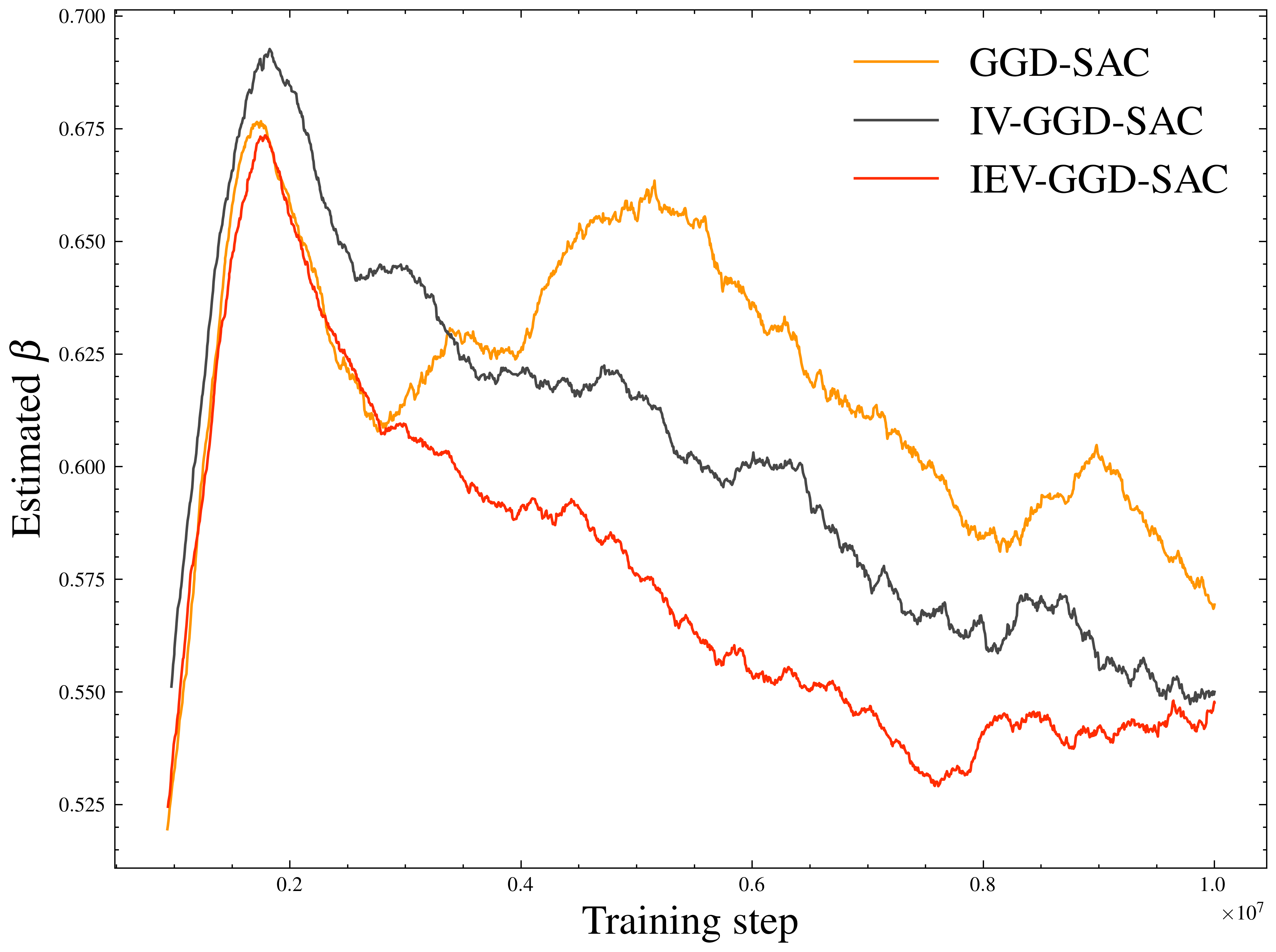
Figure 4 shows the coefficients of variation, defined as the ratio of the standard deviation to the mean, i.e., , for the variance and estimates. This statistic demonstrates the scale-invariant volatility of the parameter estimation, given that the scale of the estimated variance is significantly larger than that of the estimates. A lower coefficient of variation in estimation indicates greater stability compared to variance estimation.
The convergence of estimation is also more stable than variance estimation. This observation aligns with 1, suggesting a potential underestimation of confidence intervals in variance estimation. Considering the susceptibility of variance estimates to extreme values, such underestimation introduces considerable uncertainty in parameter estimation. Our hypothesis regarding the escalating impact of extreme TD errors throughout training is consistent with this findings, as it exacerbates the challenge in variance estimation, leading to volatility or divergence of the variance head.
These findings support that utilizing the beta head results in lower and converging coefficients of variation in parameter estimation.
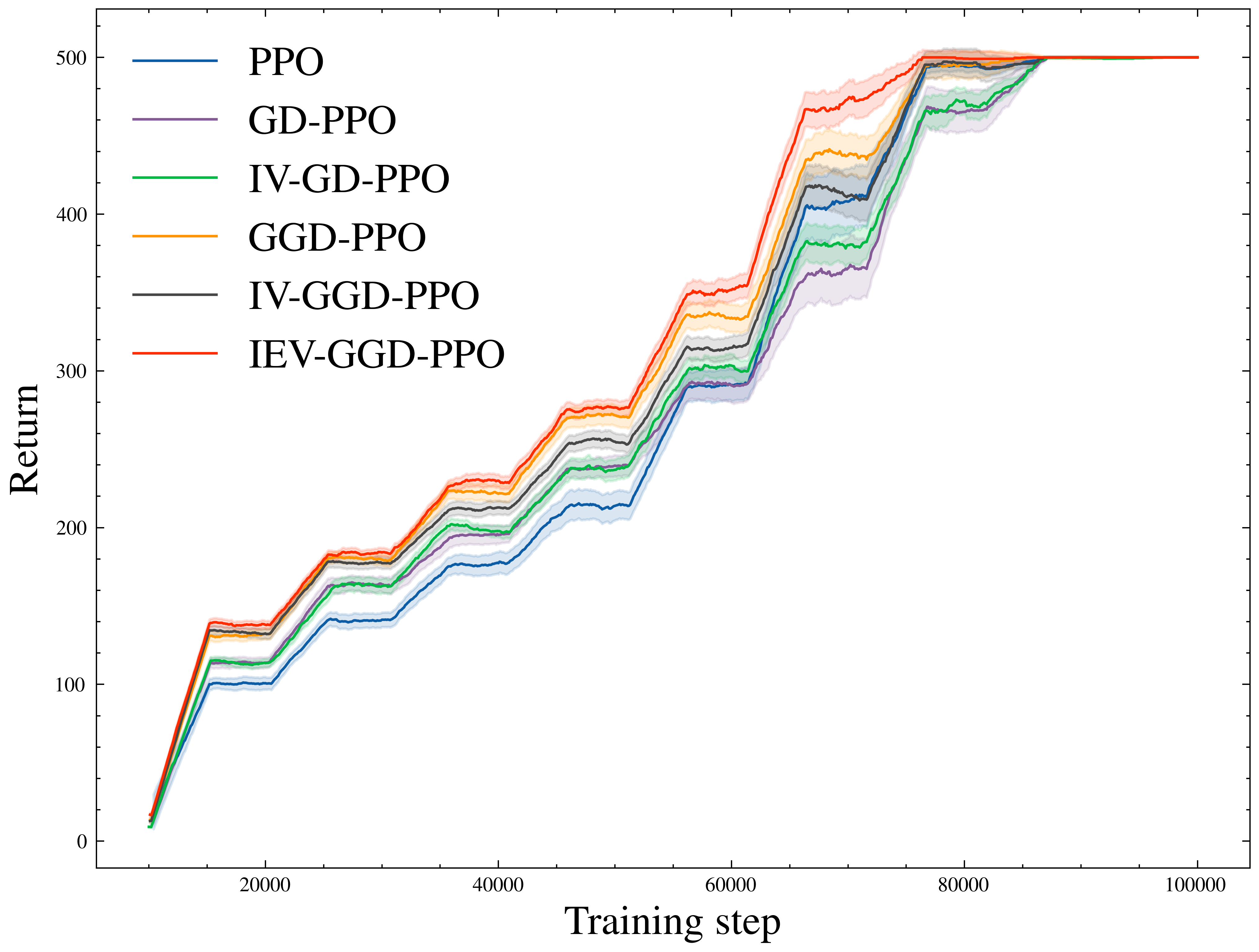
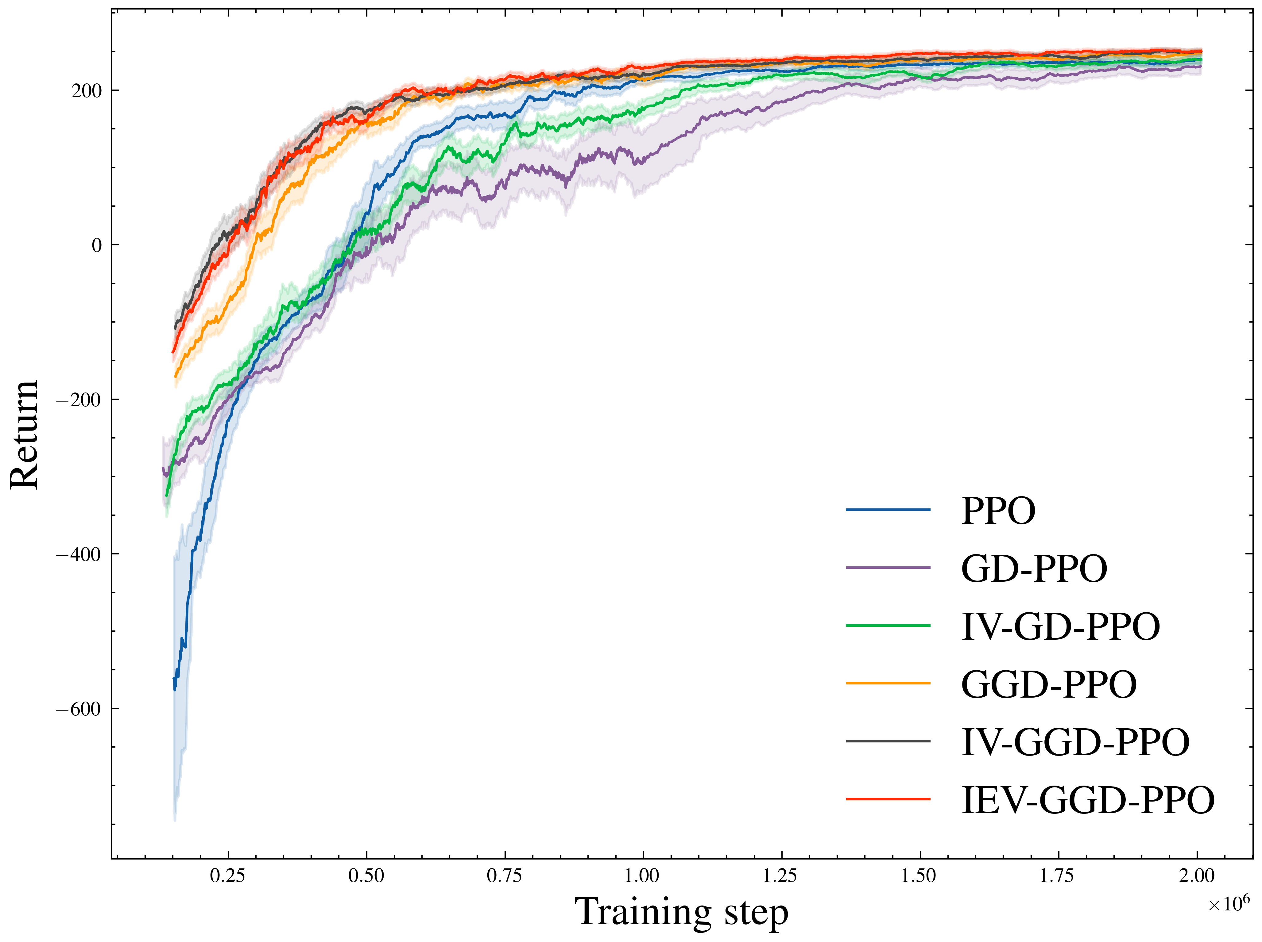
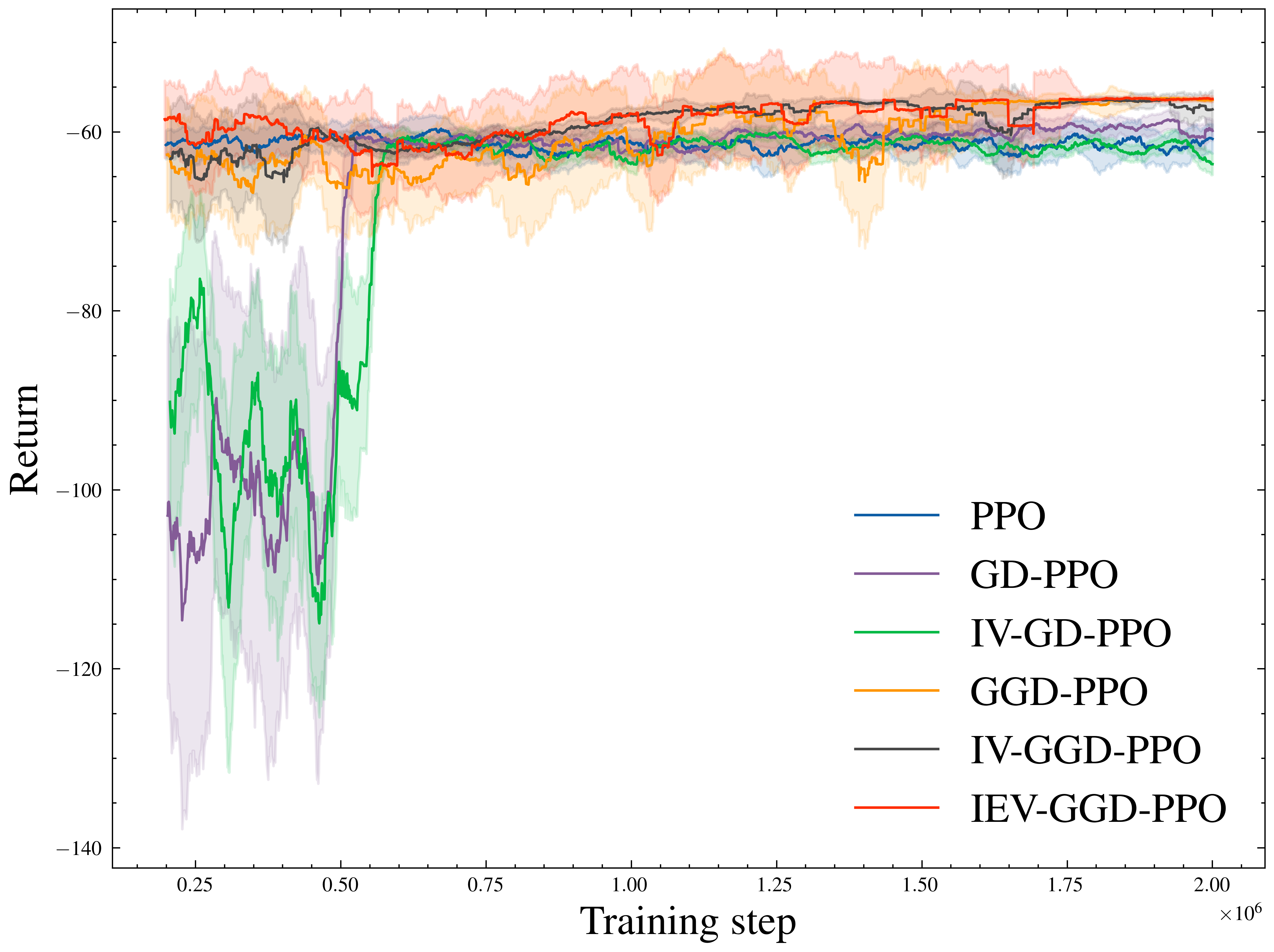
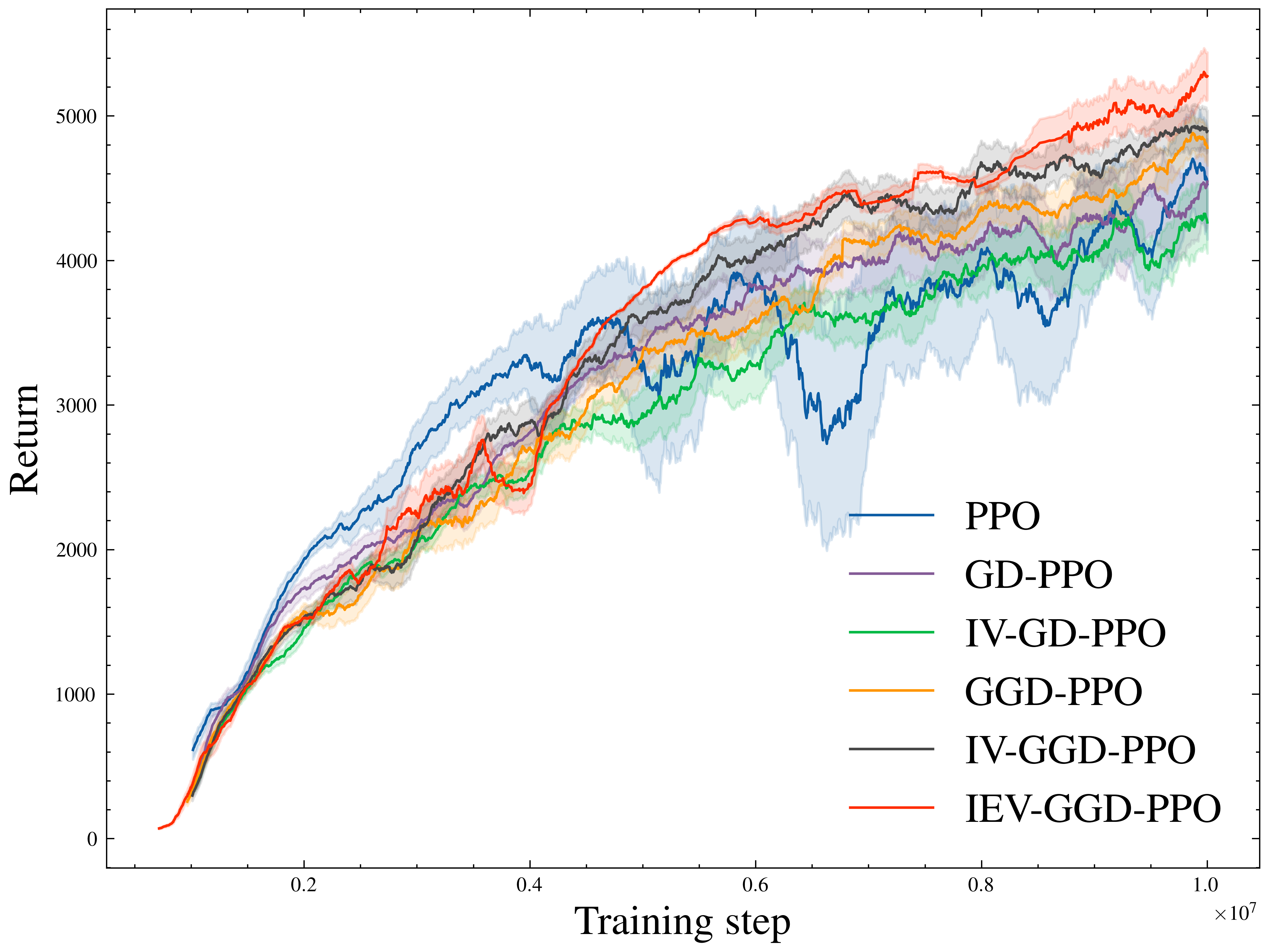
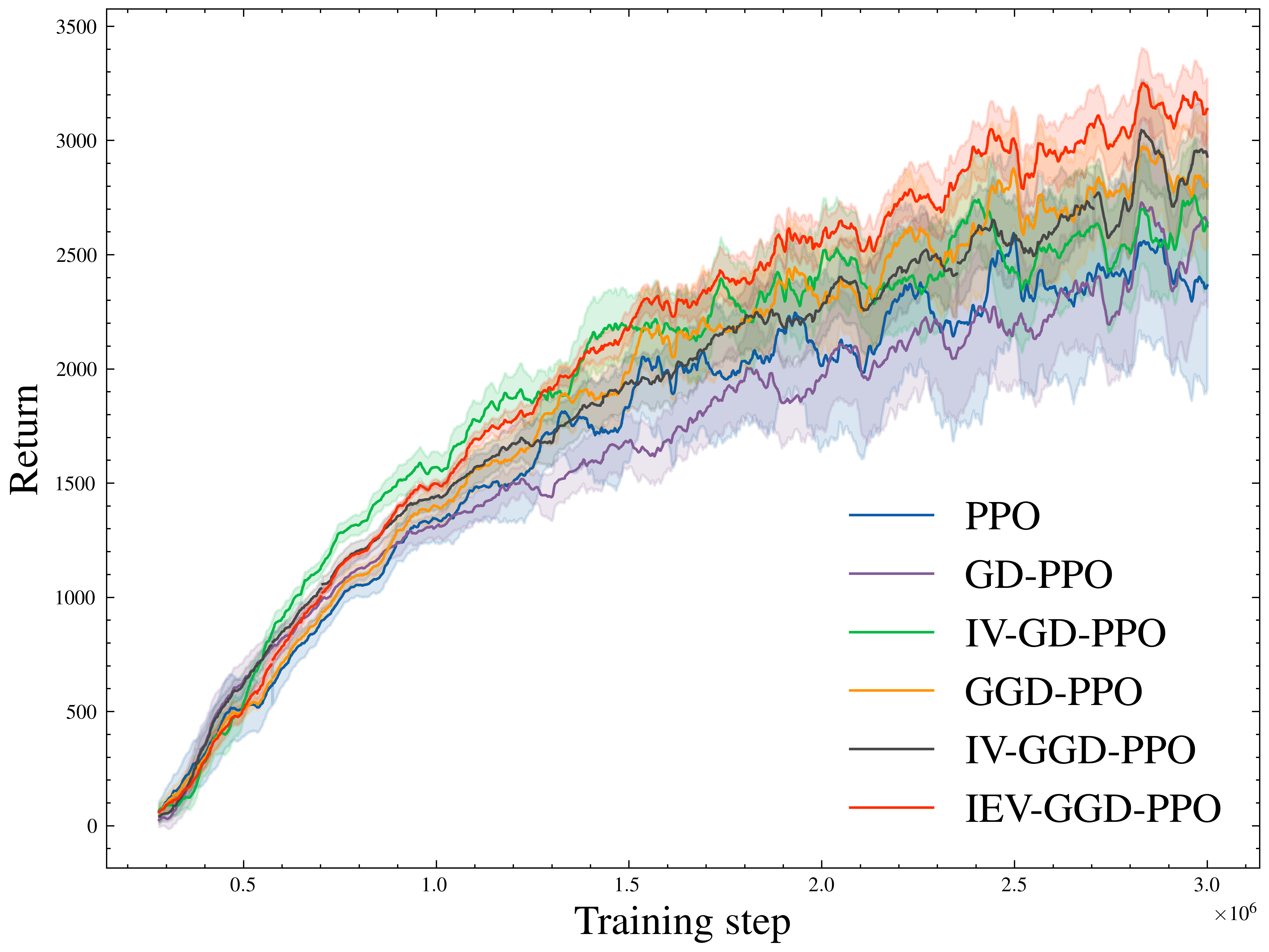
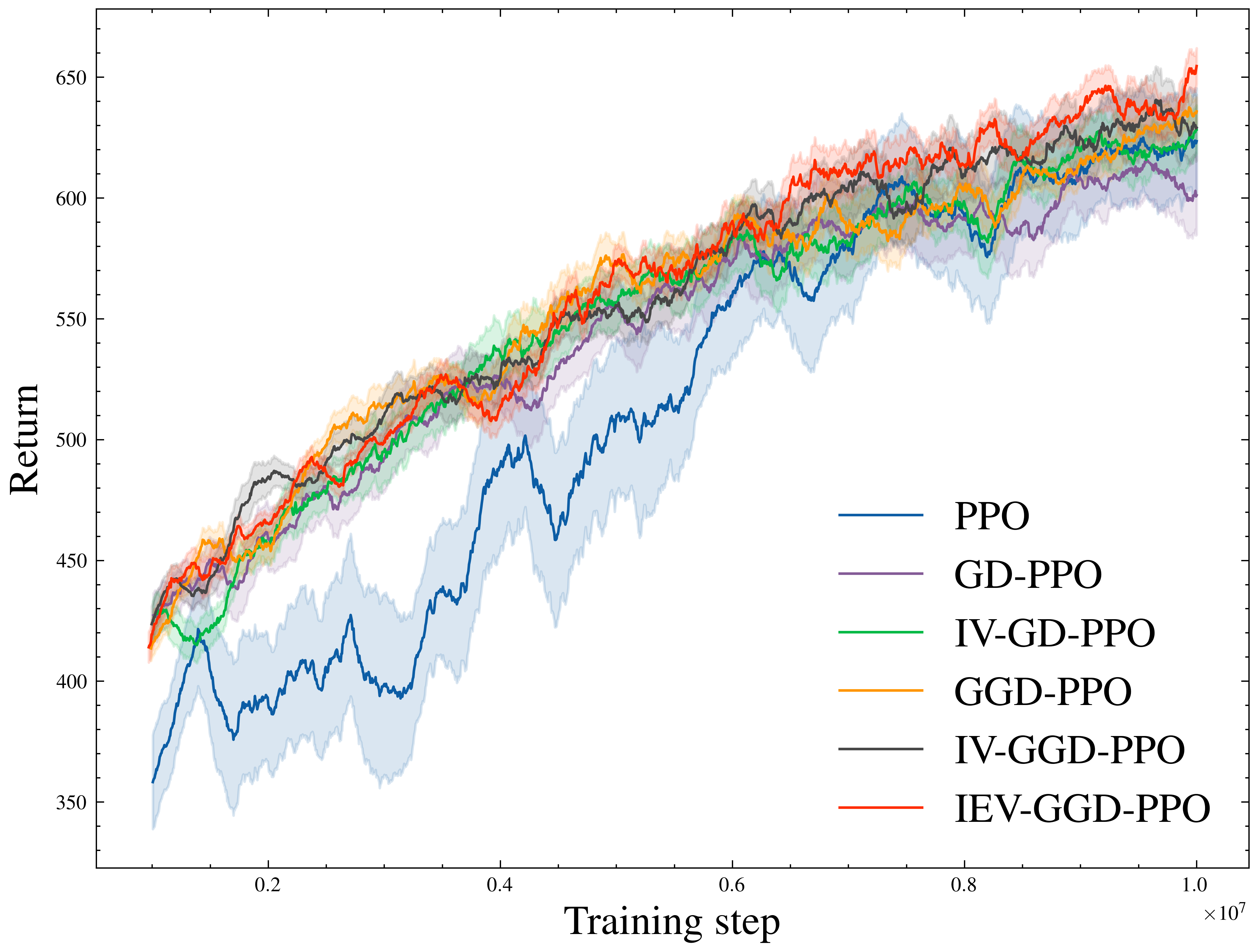
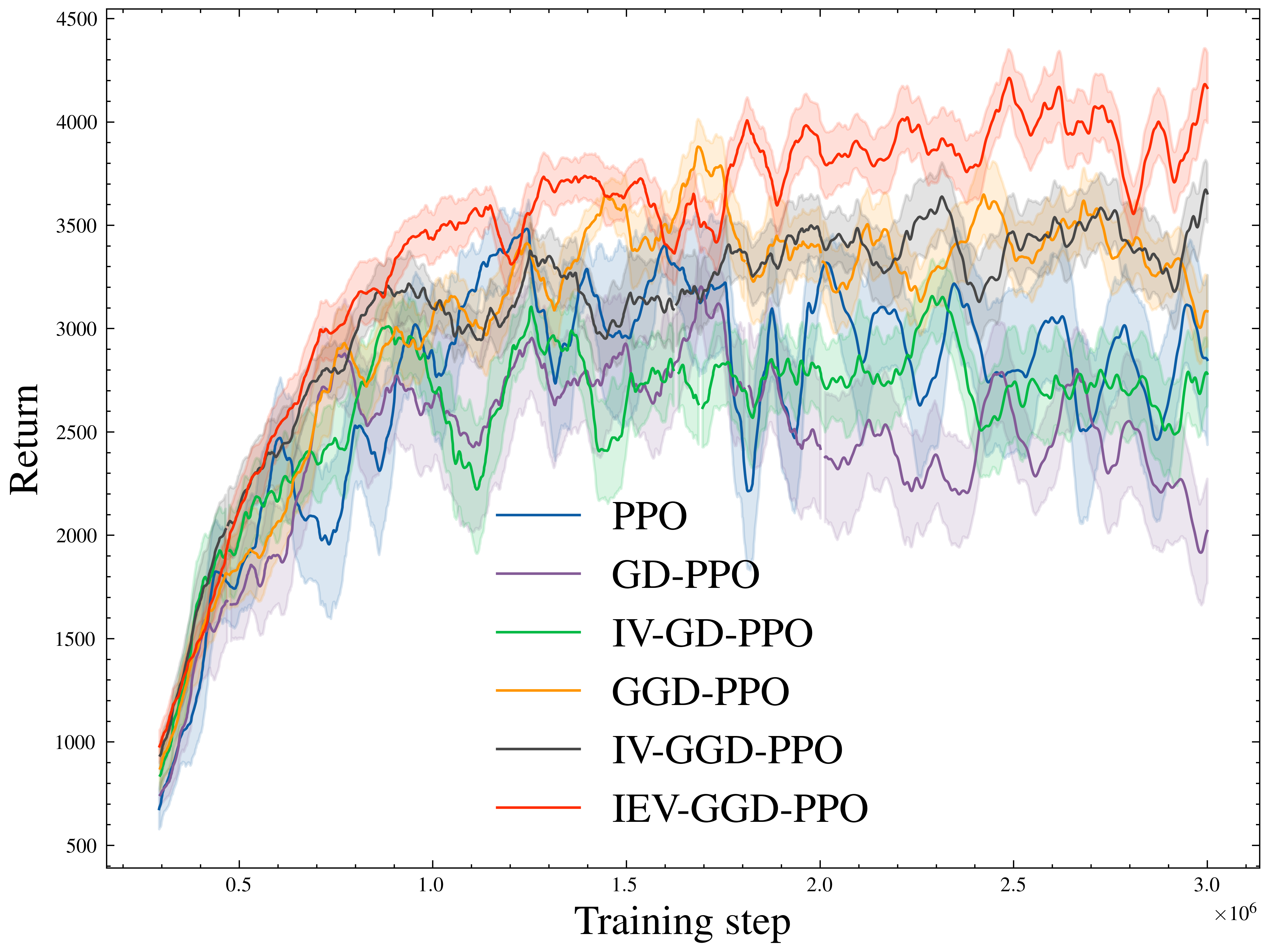
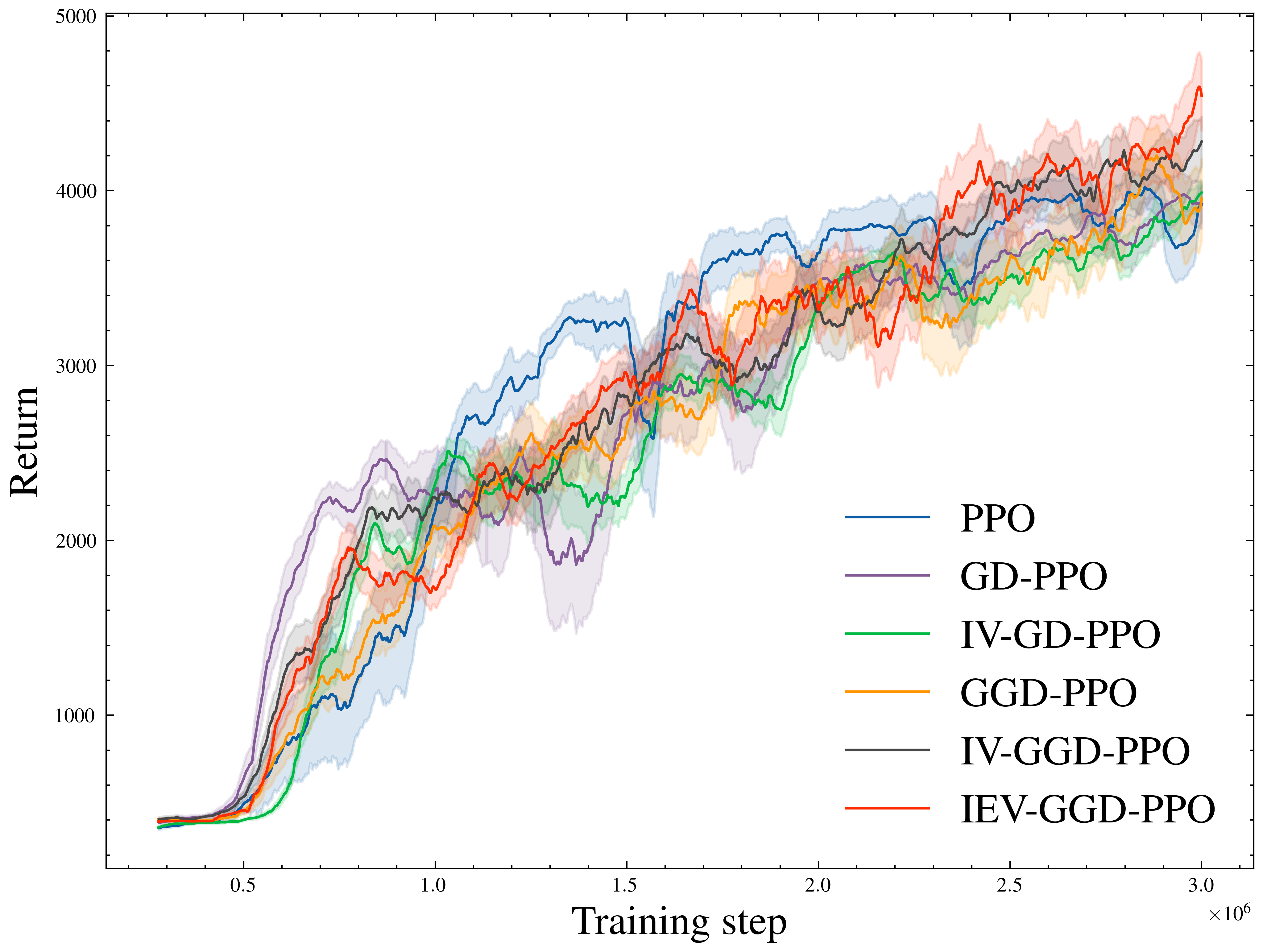
Figure 5 demonstrates the results of training PPO on MuJoCo and discrete control environments with additional noise. Remarkably, the incorporation of the beta head and BIEV regularization yields similar outcomes to those observed in SAC experiments. This indicates the efficacy of GGD error modeling in state value -based TD learning as well.
We present comprehensive ablation studies in Appendix D, examining the efficacy of key components, including risk-averse weighting, BIEV regularization applied to SAC and its Gaussian variant, and the integration of the alpha head.
5 Discussion
In this paper, we advocate for and substantiate the integration of GGD modeling for TD error analysis. Our main contribution is the introduction of a novel framework that enables robust training methodologies by leveraging the distribution’s shape. This approach accounts for both data-dependent noise, i.e., aleatoric uncertainty, and the uncertainty of value estimation, i.e., epistemic uncertainty, ultimately enhancing the model’s stability and accuracy.
Further investigation
An imperative avenue for further investigation is the application of GGD within the context of maximum entropy RL. Similar to how the Gaussian distribution maximizes entropy with constraints up to the second moment, the GGD maximizes entropy subject to a constraint on the -th absolute moment [37]. Exploring higher moments of the distribution could provide new insights into maximum entropy RL frameworks.
The absence of a comprehensive regret analysis in our current study also presents an opportunity for future work. Considering that aleatoric uncertainty in TD learning predominantly arises from reward dynamics, conducting a regret analysis on heavy-tailed TD error is warranted. This is particularly relevant as previous research has extensively studied regret in the context of heavy-tailed rewards.
While our experiments focus on policy gradient methods, the implications of TD error tailedness extend to the -learning family of algorithms. We provide empirical findings on this extension in Appendix E, which demonstrate the broader applicability of our approach. Additionally, exploring the generalized extreme value distribution could further enrich our understanding of tailedness phenomena due to its close association with extreme value theory.
Relevant applications
The implications of tailedness in TD error distributions extend into various domains, notably robust RL and risk-sensitive RL. The focus in robust RL lies on developing algorithms that are less sensitive to noise and outliers within the reward signal. Recognizing potential deviations from normality in TD error distributions is critical for designing such algorithms. Our work emphasizes the importance of considering non-normal error distributions, especially the tail behaviors, to enhance the robustness of RL algorithms.
Another significant direction is risk-sensitive RL, which seeks to assess and mitigate the risks associated with different action choices. In noisy and outlier-prone environments, capturing the risk profile using a Gaussian assumption for TD errors might be inadequate. By considering the GGD, which better models the tail behaviors of error distributions, we can develop more accurate and reliable risk-sensitive RL algorithms.
In summary, our exploration into GGD modeling of TD errors opens several promising research directions and applications, emphasizing the need to consider non-normal error distributions for enhancing the robustness and risk-sensitivity of RL algorithms.
Acknowledgments and Disclosure of Funding
We are grateful for the helpful advice provided by Dr. Heather Battey in the Department of Mathematics, Imperial College London. Her insights and feedback have been invaluable to the development and improvement of this work.
References
- [1] G. Agro. Maximum likelihood estimation for the exponential power function parameters. Communications in Statistics-Simulation and Computation, 24(2):523–536, 1995.
- [2] K. P. Balanda and H. MacGillivray. Kurtosis: a critical review. The American Statistician, 42(2):111–119, 1988.
- [3] C. M. Bishop. Mixture density networks. 1994.
- [4] S. Bochner. Stable laws of probability and completely monotone functions. 1937.
- [5] G. E. Box and G. C. Tiao. Bayesian Inference in Statistical Analysis. John Wiley & Sons, 2011.
- [6] B. D. Burch. Estimating kurtosis and confidence intervals for the variance under nonnormality. Journal of Statistical Computation and Simulation, 84(12):2710–2720, 2014.
- [7] W. J. Byun, B. Choi, S. Kim, and J. Jo. Practical application of deep reinforcement learning to optimal trade execution. FinTech, 2(3):414–429, 2023.
- [8] G. Casella and R. L. Berger. Statistical lnference. Duxbury Press, 2002.
- [9] L. Chai, J. Du, Q.-F. Liu, and C.-H. Lee. Using generalized gaussian distributions to improve regression error modeling for deep learning-based speech enhancement. IEEE/ACM Transactions on Audio, Speech, and Language Processing, 27(12):1919–1931, 2019.
- [10] W. Dabney, M. Rowland, M. Bellemare, and R. Munos. Distributional reinforcement learning with quantile regression. In Proceedings of the AAAI Conference on Artificial Intelligence, volume 32, 2018.
- [11] H. David. Robust estimation in the presence of outliers. In Robustness in Statistics, pages 61–74. Elsevier, 1979.
- [12] L. T. DeCarlo. On the meaning and use of kurtosis. Psychological Methods, 2(3):292, 1997.
- [13] S. Depeweg, J.-M. Hernandez-Lobato, F. Doshi-Velez, and S. Udluft. Decomposition of uncertainty in bayesian deep learning for efficient and risk-sensitive learning. In International conference on machine learning, pages 1184–1193. PMLR, 2018.
- [14] A. Der Kiureghian and O. Ditlevsen. Aleatory or epistemic? does it matter? Structural Safety, 31(2):105–112, 2009.
- [15] C. Dugas, Y. Bengio, F. Bélisle, C. Nadeau, and R. Garcia. Incorporating second-order functional knowledge for better option pricing. Advances in Neural Information Processing Systems, 13, 2000.
- [16] A. Dytso, R. Bustin, H. V. Poor, and S. Shamai. Analytical properties of generalized gaussian distributions. Journal of Statistical Distributions and Applications, 5:1–40, 2018.
- [17] M. Emamifar and S. F. Ghoreishi. Uncertainty-aware reinforcement learning for safe control of autonomous vehicles in signalized intersections. In 2023 IEEE Conference on Artificial Intelligence (CAI), pages 81–82. IEEE, 2023.
- [18] T. S. Ferguson. A Course in Large Sample Theory. Routledge, 2017.
- [19] R. A. Fisher and L. H. C. Tippett. Limiting forms of the frequency distribution of the largest or smallest member of a sample. In Mathematical Proceedings of the Cambridge Philosophical Society, volume 24, pages 180–190. Cambridge University Press, 1928.
- [20] S. Flennerhag, J. X. Wang, P. Sprechmann, F. Visin, A. Galashov, S. Kapturowski, D. L. Borsa, N. Heess, A. Barreto, and R. Pascanu. Temporal difference uncertainties as a signal for exploration. arXiv preprint arXiv:2010.02255, 2020.
- [21] S. Fujimoto, H. Hoof, and D. Meger. Addressing function approximation error in actor-critic methods. In International Conference on Machine Learning, pages 1587–1596. PMLR, 2018.
- [22] D. Garg, J. Hejna, M. Geist, and S. Ermon. Extreme q-learning: Maxent rl without entropy. In The Eleventh International Conference on Learning Representations, 2022.
- [23] U. Gather and B. K. Kale. Maximum likelihood estimation in the presence of outiliers. Communications in Statistics-Theory and Methods, 17(11):3767–3784, 1988.
- [24] M. Giacalone. A combined method based on kurtosis indexes for estimating p in non-linear lp-norm regression. Sustainable Futures, 2:100008, 2020.
- [25] G. L. Giller. A generalized error distribution. 2005.
- [26] T. Haarnoja, A. Zhou, P. Abbeel, and S. Levine. Soft actor-critic: Off-policy maximum entropy deep reinforcement learning with a stochastic actor. In International Conference on Machine Learning, pages 1861–1870. PMLR, 2018.
- [27] C.-J. Hoel, K. Wolff, and L. Laine. Ensemble quantile networks: Uncertainty-aware reinforcement learning with applications in autonomous driving. IEEE Transactions on Intelligent Transportation Systems, 2023.
- [28] D. Y.-T. Hui, A. C. Courville, and P.-L. Bacon. Double gumbel q-learning. Advances in Neural Information Processing Systems, 36, 2023.
- [29] D. Janz, J. Hron, P. Mazur, K. Hofmann, J. M. Hernández-Lobato, and S. Tschiatschek. Successor uncertainties: exploration and uncertainty in temporal difference learning. Advances in Neural Information Processing Systems, 32, 2019.
- [30] G. Kahn, A. Villaflor, V. Pong, P. Abbeel, and S. Levine. Uncertainty-aware reinforcement learning for collision avoidance. arXiv preprint arXiv:1702.01182, 2017.
- [31] A. Kendall and Y. Gal. What uncertainties do we need in bayesian deep learning for computer vision? Advances in Neural Information Processing Systems, 30, 2017.
- [32] J. Kleffe. Some remarks on improving unbiased estimators by multiplication with a constant. In Linear Statistical Inference: Proceedings of the International Conference held at Poznań, Poland, June 4–8, 1984, pages 150–161. Springer, 1985.
- [33] B. Lakshminarayanan, A. Pritzel, and C. Blundell. Simple and scalable predictive uncertainty estimation using deep ensembles. Advances in Neural Information Processing Systems, 30, 2017.
- [34] H. Levy. Stochastic dominance and expected utility: Survey and analysis. Management Science, 38(4):555–593, 1992.
- [35] L. Liang, Y. Xu, S. McAleer, D. Hu, A. Ihler, P. Abbeel, and R. Fox. Reducing variance in temporal-difference value estimation via ensemble of deep networks. In International Conference on Machine Learning, pages 13285–13301. PMLR, 2022.
- [36] O. Lockwood and M. Si. A review of uncertainty for deep reinforcement learning. In Proceedings of the AAAI Conference on Artificial Intelligence and Interactive Digital Entertainment, volume 18, pages 155–162, 2022.
- [37] D. J. MacKay. Information Theory, Inference and Learning Algorithms. Cambridge university press, 2003.
- [38] V. Mai, K. Mani, and L. Paull. Sample efficient deep reinforcement learning via uncertainty estimation. In International Conference on Learning Representations, 2022.
- [39] J. Martin, M. Lyskawinski, X. Li, and B. Englot. Stochastically dominant distributional reinforcement learning. In International Conference on Machine Learning, pages 6745–6754. PMLR, 2020.
- [40] A. Mavor-Parker, K. Young, C. Barry, and L. Griffin. How to stay curious while avoiding noisy tvs using aleatoric uncertainty estimation. In International Conference on Machine Learning, pages 15220–15240. PMLR, 2022.
- [41] T. K. Milton, R. O. Odhiambo, and G. O. Orwa. Estimation of population variance using the coefficient of kurtosis and median of an auxiliary variable under simple random sampling. Open Journal of Statistics, 7:944–955, 2017.
- [42] V. Mnih, A. P. Badia, M. Mirza, A. Graves, T. Lillicrap, T. Harley, D. Silver, and K. Kavukcuoglu. Asynchronous methods for deep reinforcement learning. In International Conference on Machine Learning, pages 1928–1937. PMLR, 2016.
- [43] V. Mnih, K. Kavukcuoglu, D. Silver, A. A. Rusu, J. Veness, M. G. Bellemare, A. Graves, M. Riedmiller, A. K. Fidjeland, G. Ostrovski, et al. Human-level control through deep reinforcement learning. Nature, 518(7540):529–533, 2015.
- [44] A. M. Mood. Introduction to the Theory of Statistics. McGraw-hill, 1950.
- [45] J. Moody and M. Saffell. Reinforcement learning for trading. Advances in Neural Information Processing Systems, 11, 1998.
- [46] S. Nadarajah. A generalized normal distribution. Journal of Applied Statistics, 32(7):685–694, 2005.
- [47] D. A. Nix and A. S. Weigend. Estimating the mean and variance of the target probability distribution. In Proceedings of 1994 IEEE International Conference on Neural Networks (ICNN’94), volume 1, pages 55–60. IEEE, 1994.
- [48] M. Novey, T. Adali, and A. Roy. A complex generalized gaussian distribution—characterization, generation, and estimation. IEEE Transactions on Signal Processing, 58(3):1427–1433, 2009.
- [49] I. Osband and B. Van Roy. Gaussian-dirichlet posterior dominance in sequential learning. arXiv preprint arXiv:1702.04126, 2017.
- [50] A. Paszke, S. Gross, F. Massa, A. Lerer, J. Bradbury, G. Chanan, T. Killeen, Z. Lin, N. Gimelshein, L. Antiga, et al. Pytorch: An imperative style, high-performance deep learning library. Advances in Neural Information Processing Systems, 32, 2019.
- [51] A. Raffin, A. Hill, A. Gleave, A. Kanervisto, M. Ernestus, and N. Dormann. Stable-baselines3: Reliable reinforcement learning implementations. Journal of Machine Learning Research, 22(268):1–8, 2021.
- [52] J. Schulman, F. Wolski, P. Dhariwal, A. Radford, and O. Klimov. Proximal policy optimization algorithms. arXiv preprint arXiv:1707.06347, 2017.
- [53] D. T. Searls and P. Intarapanich. A note on an estimator for the variance that utilizes the kurtosis. The American Statistician, 44(4):295–296, 1990.
- [54] M. Seitzer, A. Tavakoli, D. Antic, and G. Martius. On the pitfalls of heteroscedastic uncertainty estimation with probabilistic neural networks. In International Conference on Learning Representations, 2022.
- [55] B. Shahriari, A. Abdolmaleki, A. Byravan, A. Friesen, S. Liu, J. T. Springenberg, N. Heess, M. Hoffman, and M. Riedmiller. Revisiting gaussian mixture critics in off-policy reinforcement learning: a sample-based approach. arXiv preprint arXiv:2204.10256, 2022.
- [56] S. Sun, R. Wang, and B. An. Reinforcement learning for quantitative trading. ACM Transactions on Intelligent Systems and Technology, 14(3):1–29, 2023.
- [57] R. S. Sutton. Learning to predict by the methods of temporal differences. Machine Learning, 3:9–44, 1988.
- [58] R. S. Sutton and A. G. Barto. Reinforcement Learning: An Introduction. MIT Press, 2018.
- [59] E. Todorov, T. Erez, and Y. Tassa. Mujoco: A physics engine for model-based control. In 2012 IEEE/RSJ International Conference on Intelligent Robots and Systems, pages 5026–5033. IEEE, 2012.
- [60] M. Towers, J. K. Terry, A. Kwiatkowski, J. U. Balis, G. d. Cola, T. Deleu, M. Goulão, A. Kallinteris, A. KG, M. Krimmel, R. Perez-Vicente, A. Pierré, S. Schulhoff, J. J. Tai, A. T. J. Shen, and O. G. Younis. Gymnasium, Mar. 2023.
- [61] U. Upadhyay, Y. Chen, and Z. Akata. Robustness via uncertainty-aware cycle consistency. Advances in Neural Information Processing Systems, 34:28261–28273, 2021.
- [62] N. G. Ushakov. Selected Topics in Characteristic Functions. Walter de Gruyter, 2011.
- [63] M. Valdenegro-Toro and D. S. Mori. A deeper look into aleatoric and epistemic uncertainty disentanglement. In 2022 IEEE/CVF Conference on Computer Vision and Pattern Recognition Workshops (CVPRW), pages 1508–1516. IEEE, 2022.
- [64] P. Virtanen, R. Gommers, T. E. Oliphant, M. Haberland, T. Reddy, D. Cournapeau, E. Burovski, P. Peterson, W. Weckesser, J. Bright, et al. Scipy 1.0: fundamental algorithms for scientific computing in python. Nature Methods, 17(3):261–272, 2020.
- [65] M. Vlastelica, S. Blaes, C. Pinneri, and G. Martius. Risk-averse zero-order trajectory optimization. In 5th Annual Conference on Robot Learning, 2021.
- [66] S. D. Walter, J. Rychtář, D. Taylor, and N. Balakrishnan. Estimation of standard deviations and inverse-variance weights from an observed range. Statistics in Medicine, 41(2):242–257, 2022.
- [67] E. Wencheko and H. W. Chipoyera. Estimation of the variance when kurtosis is known. Statistical Papers, 50:455–464, 2009.
- [68] K.-H. Yuan, P. M. Bentler, and W. Zhang. The effect of skewness and kurtosis on mean and covariance structure analysis: The univariate case and its multivariate implication. Sociological Methods & Research, 34(2):240–258, 2005.
- [69] R. Zeckhauser and M. Thompson. Linear regression with non-normal error terms. The Review of Economics and Statistics, pages 280–286, 1970.
Appendix A Extended results
A.1 Temporal difference error plots
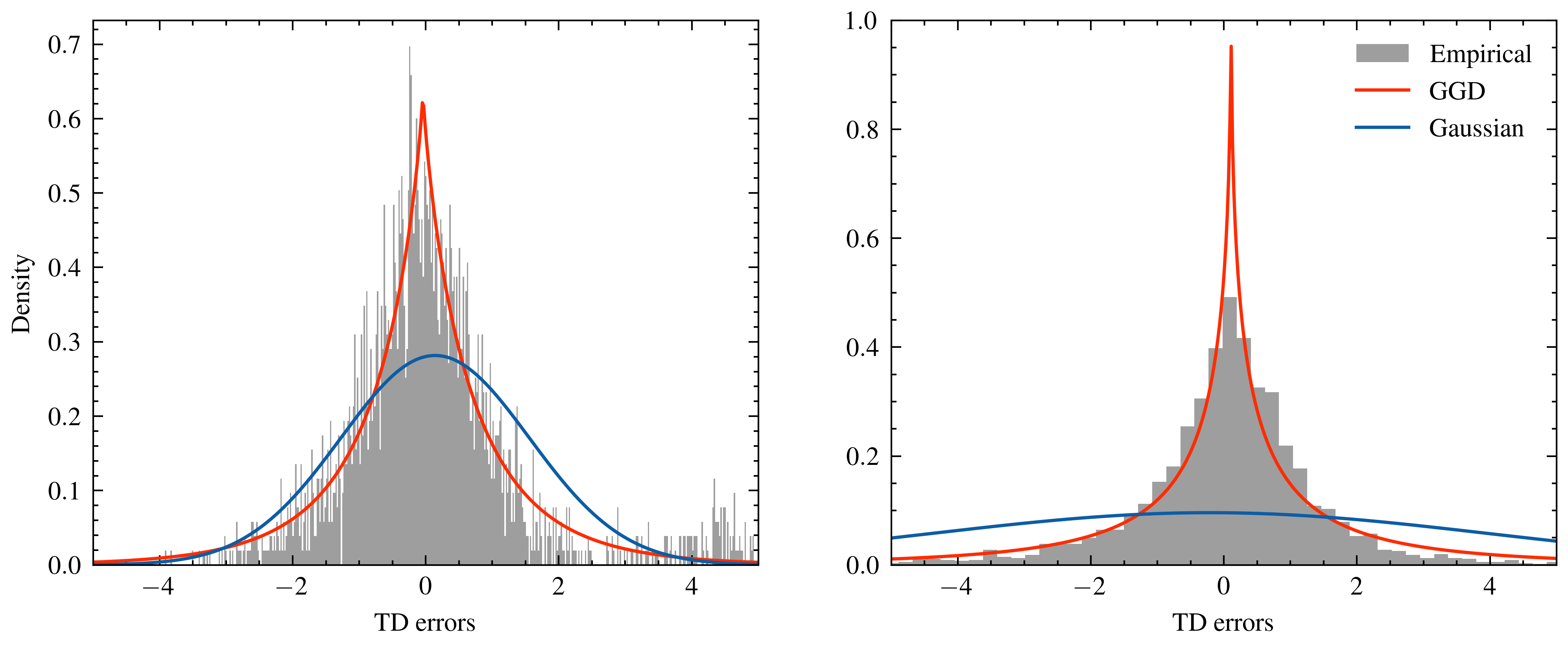
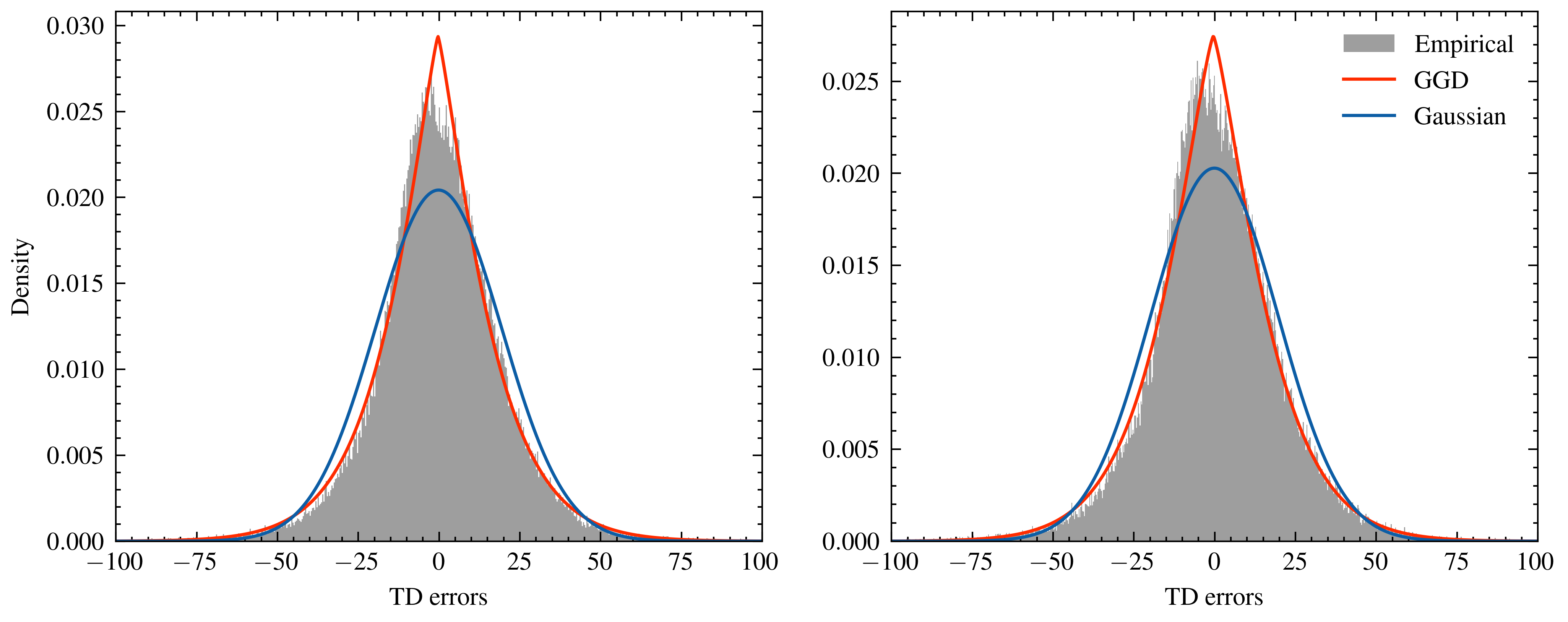
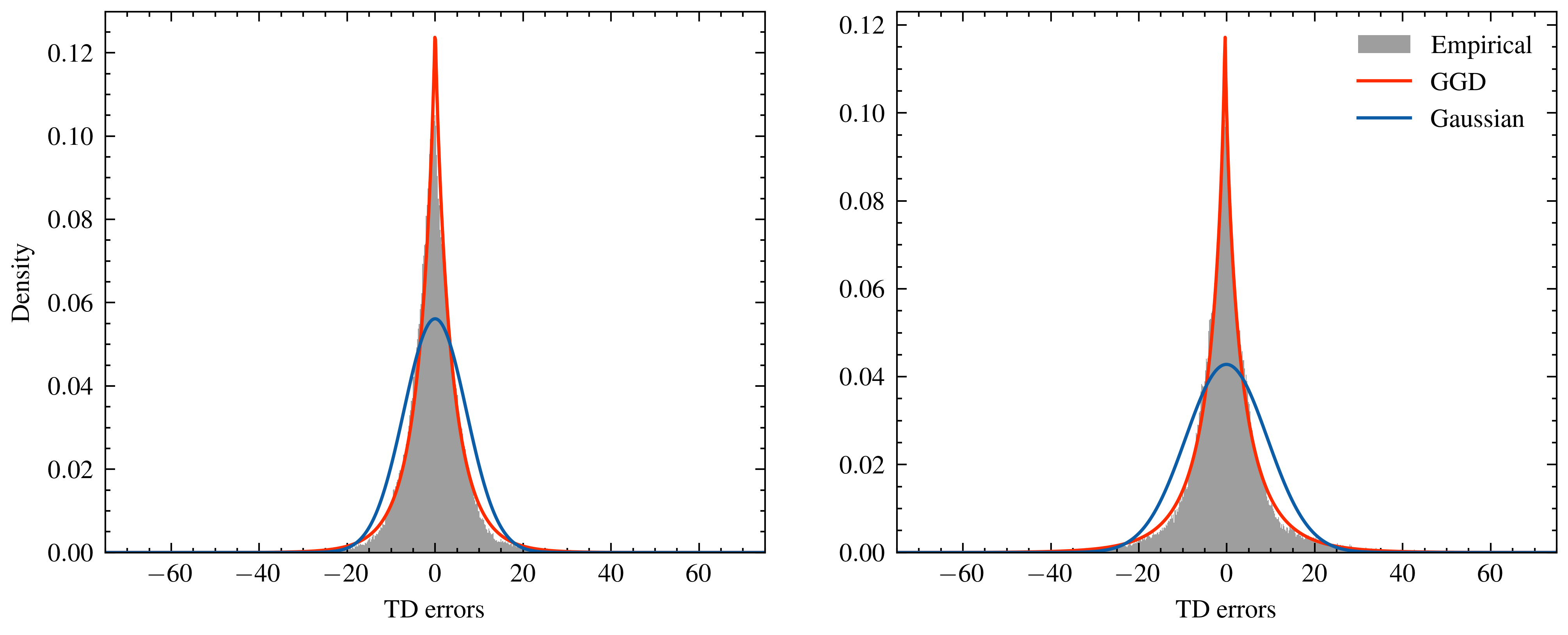
We present the distributions of TD errors sampled at the initial and final evaluation steps, depicted in Figures 2 and 6 for SAC, and Figure 7 for PPO, which highlights the heavy tailedness of TD errors and the tendency converge to heavy tail throughout training. This finding also emphasizes how aleatoric uncertainty affects their distribution, as elaborated in Section 3.1. Interestingly, both state-action values and state values demonstrate similar characteristics in their TD error distributions.
A.2 Coefficients of variation of parameter estimation
A.3 PPO on other environments
A.4 estimation
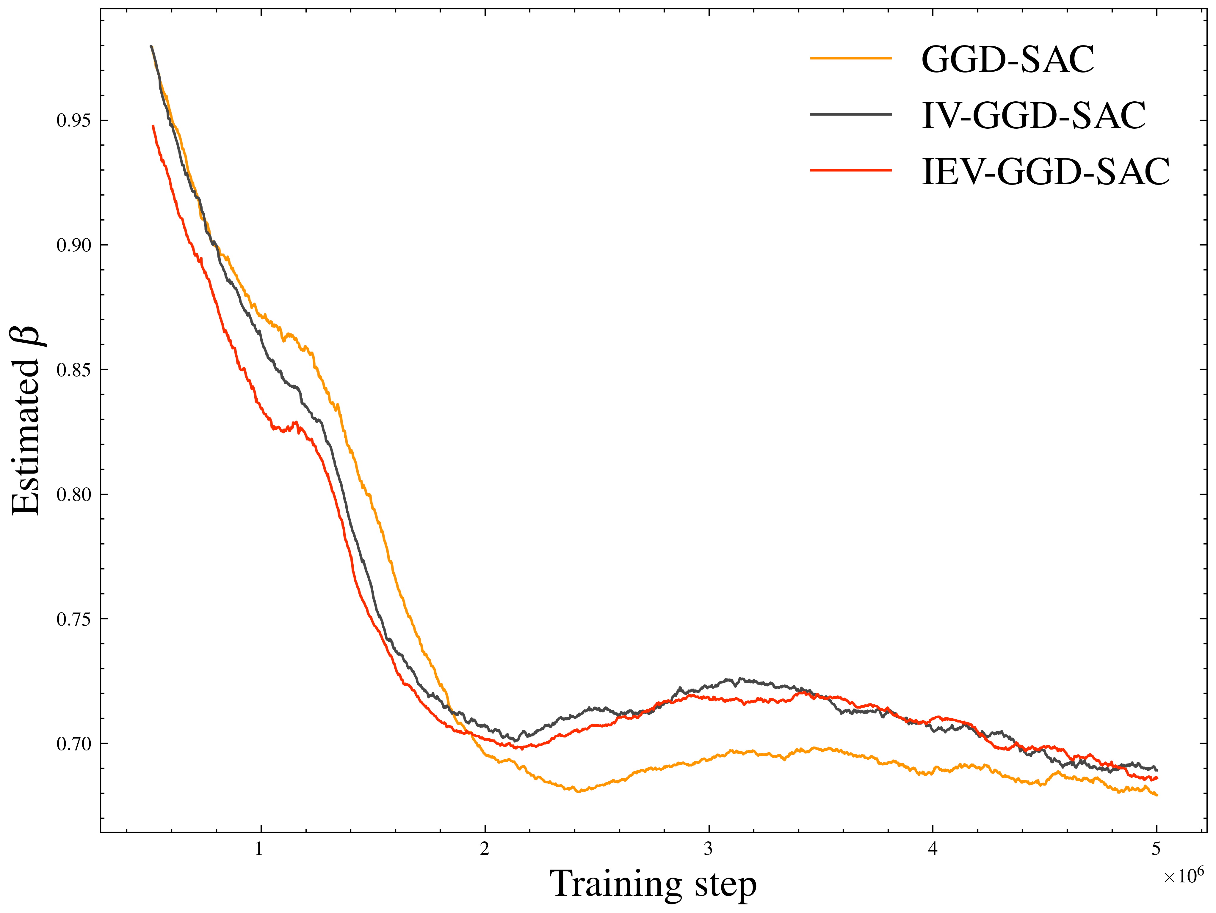
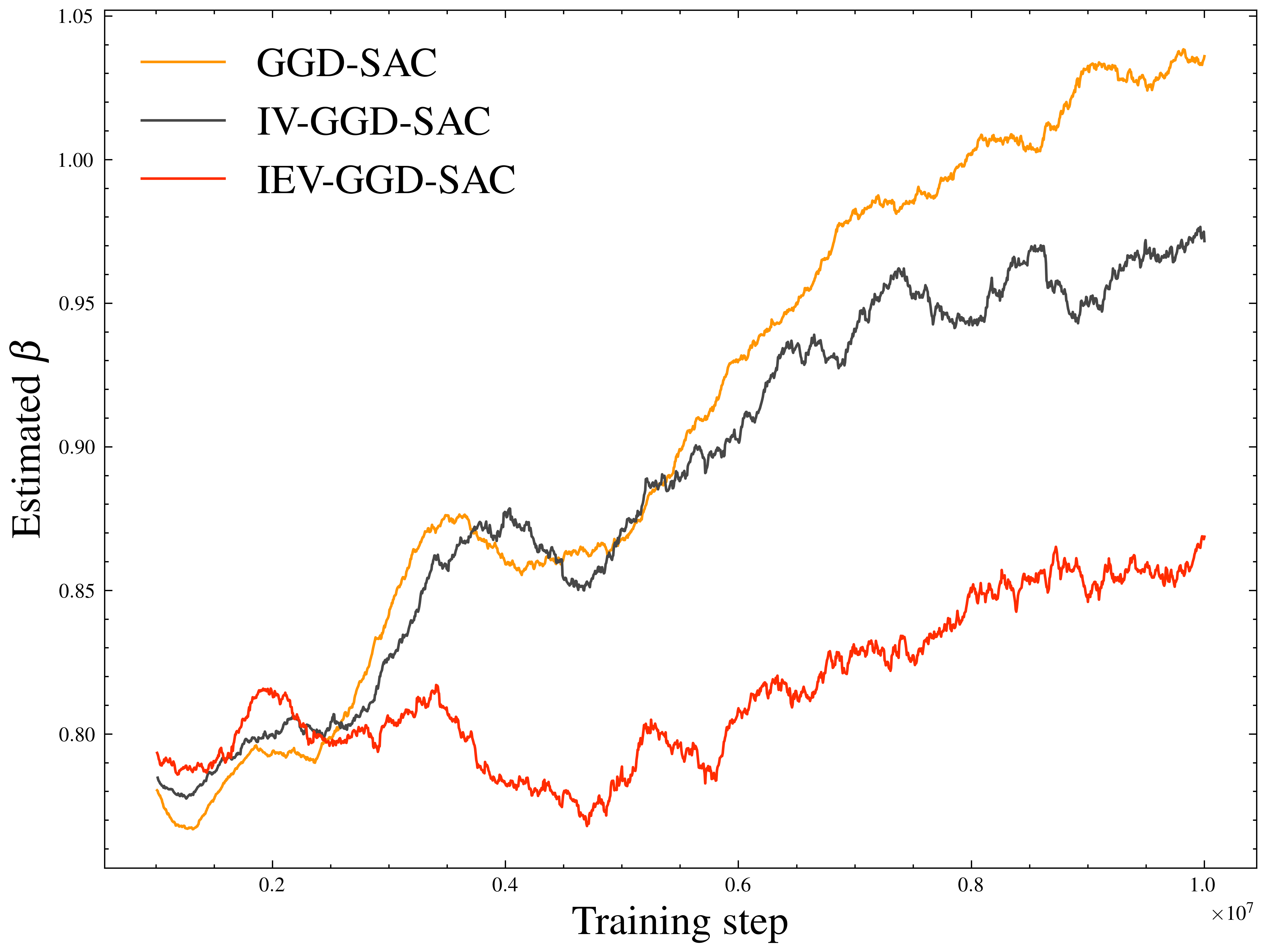
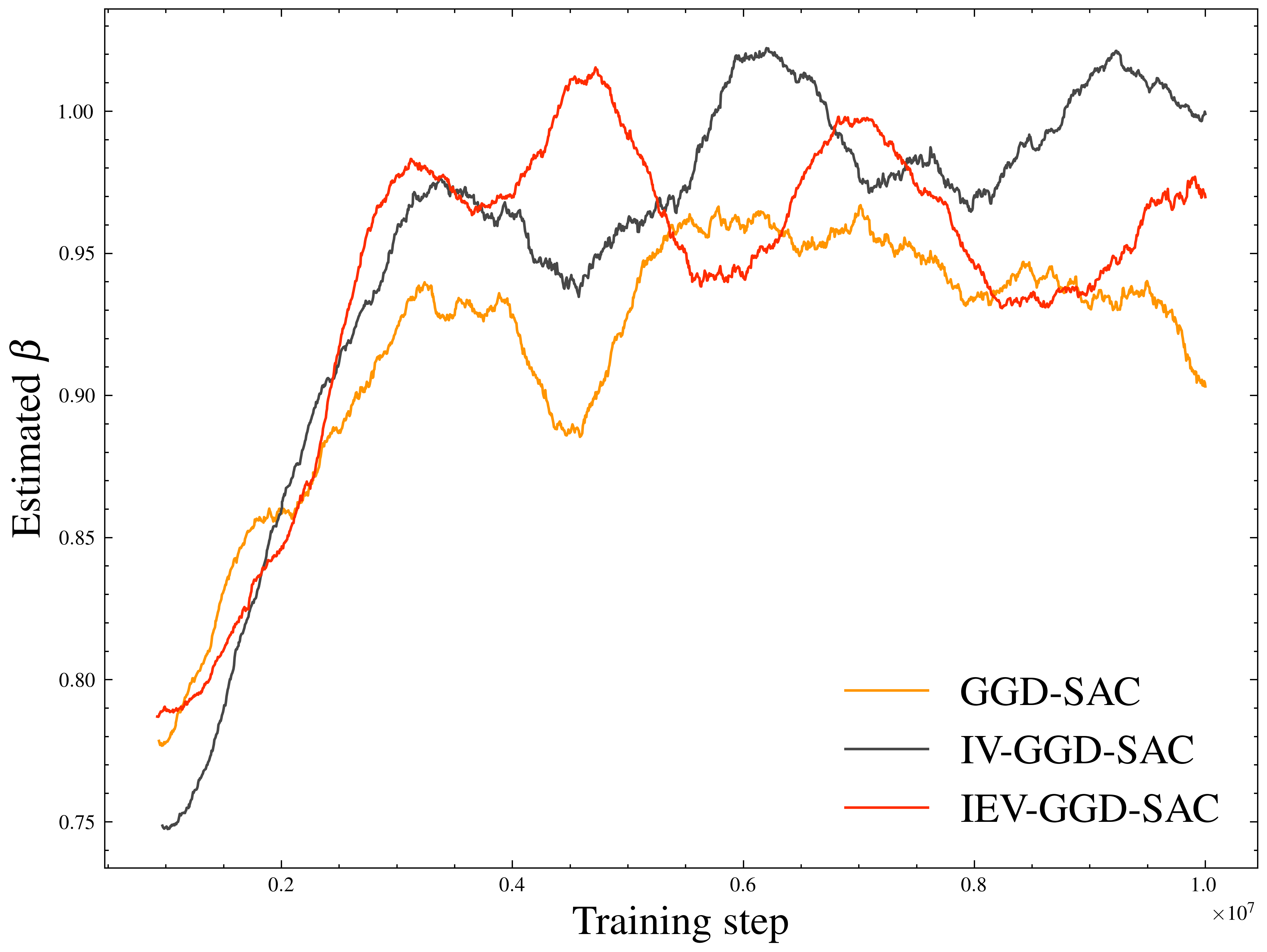
The parameter estimates from the beta distribution reveal consistently low values of across all environments, indicating a leptokurtic TD error distribution, as depicted in Figure 10. These findings align with the observations from the TD error plots, where TD errors exhibit a closer resemblance to the GGD rather than a Gaussian distribution.
Appendix B Proofs
B.1 Of 1
Proof.
Consider a finite sample of independent, normally distributed random variables with , where represents the true generative parameters. Under this assumption, both skewness and kurtosis are zero. Consequently, the moments are given by , , and .
Assuming , where denotes the convergence in probability, under appropriate regularity conditions, then the asymptotic normality theorem of Cramer leads to
as [18]. Here, is the Fisher information matrix.
Through straightforward calculations involving the log likelihood function derivatives, we obtain
Thus, as , .
Now, consider a finite sample of independent, non-normally distributed random variables, with MLE estimator . By applying analogous reasoning, we seek the asymptotic distribution of . Letting gives us
Therefore, as ,
| (11) | ||||
Denoting , (11) states that and are asymptotically equivalent, i.e.,
By Slutsky’s theorem [18], has the same asymptotic normality as , i.e.,
where is a covariance matrix with
From the equality between and , we find that
Hence, when normality is assumed for non-normally distributed data, the bias of the standard error estimate based on depends on , i.e., negative when and positive when . ∎
B.2 Of 1
To prove that the NLL function of GGD is well defined for , we show that the PDF of GGD is everywhere positive with it being a positive definite function. An easy but effective proof can be done by demonstrating that the PDF of GGD for is equivalent to the characteristic function of an -stable distribution, up to a normalizing constant [16]. Given the positive definiteness of all characteristic functions [16, 62], this equivalence assures the positive definiteness of the GGD PDF. However, we offer a proof rooted in the properties of the positive definite function class.
Proof.
To demonstrate the positive definiteness of the GGD PDF, it is sufficient to show the positivity of the function:
where .
For a class of positive definite functions , which can be interpreted as Fourier transforms of bounded non-negative distributions, the function , i.e.,
satisfy the following properties:
-
1.
For any non-negative scalars and functions , .
-
2.
For , .
-
3.
If a sequence of functions converges uniformly in every finite interval, then the limit function .
Now, let , and we aim to prove that belongs to for , excluding the trivial case . Since for ,
can be expressed as a uniform limit of functions , where each takes the form:
for some sequences and with .
By simplifying, we find that for some and and letting :
Note that from Taylor expansions.
From the properties of a positive definite function class, it is now sufficient to show that belongs to to prove . We demonstrate this by expressing it as a Fourier transform of a bounded non-negative distribution:
∎
B.3 Of 2
Proof.
For random variable , its cumulative distribution function is defined as
where
represent the gamma function and lower incomplete gamma function for a complex parameter with a positive real part.
Expanding the left-hand side of (7), we obtain
| (12) | ||||
Defining , we aim to demonstrate the monotonicity of to conclude the proof, as monotonically increasing leads to for , i.e., the integral in (12) is greater than or equal to zero.
With the definition of the gamma and lower incomplete gamma function,
| (13) |
Employing integration by substitution with , (13) transforms to
The function is thus increasing if, for and any ,
which follows from the monotonicity of the exponential function [16].
Consequently, , implying that (12) is greater than or equal to zero. ∎
B.4 Of 2
Proof.
It is well known that the variance of the unbiased estimator is given by
And the MSE of a biased estimator is
| (14) |
By differentiating (14) with respect to , we can calculate the optimal value with minimal as
Therefore,
It is easy to show that this is the optimal value, given that the second derivative is positive, i.e.,
∎
Appendix C Experimental details
All experiments are conducted on a computational infrastructure consisting of 8 NVIDIA A100 80GB PCIe GPUs and 256 AMD EPYC™ 7742 processors. Further details on the software setup can be accessed on GitHub111https://github.com/ait-lab/ggtde.
Additional noise
To extend our study to discrete control scenarios, we enhance the baseline environments with stochastic perturbations. In CartPole-v1 and MountainCar-v0, we introduce uniform noise to manipulate forces or torques. Furthermore, in LunarLander-v2, wind dynamics are activated. For a comprehensive analysis of how wind impacts the LunarLander-v2 dynamics, please consult the official documentation222https://gymnasium.farama.org/environments/box2d/lunar_lander.
Implementation
To bolster numerical stability and enforce positivity constraints, we utilize the softplus function, a smooth approximation to the ReLU function [15], on the outputs from the variance or beta head. Furthermore, we modify the NLL loss for the GGD by employing as a multiplier instead of an exponent:
Although this adaptation does not precisely mirror the genuine NLL loss of the GGD, the discrepancy in computed loss between the original and modified forms remains negligible across practical ranges of the TD error and . This modification offers a practical advantage by addressing the issue of flat regions in the original loss function, thus providing more informative gradients for model updates. Importantly, it should be noted that despite this adjustment, the positive-definiteness ensured by 1 remains intact, as the modification preserves proportionality to the original loss with set to 1. This promotes the stability and convergence properties crucial for error modeling based on GGD.
Appendix D Ablation studies
We conduct a series of ablation studies using the SAC algorithm across selected MuJoCo environments.
D.1 On risk-averse weighting
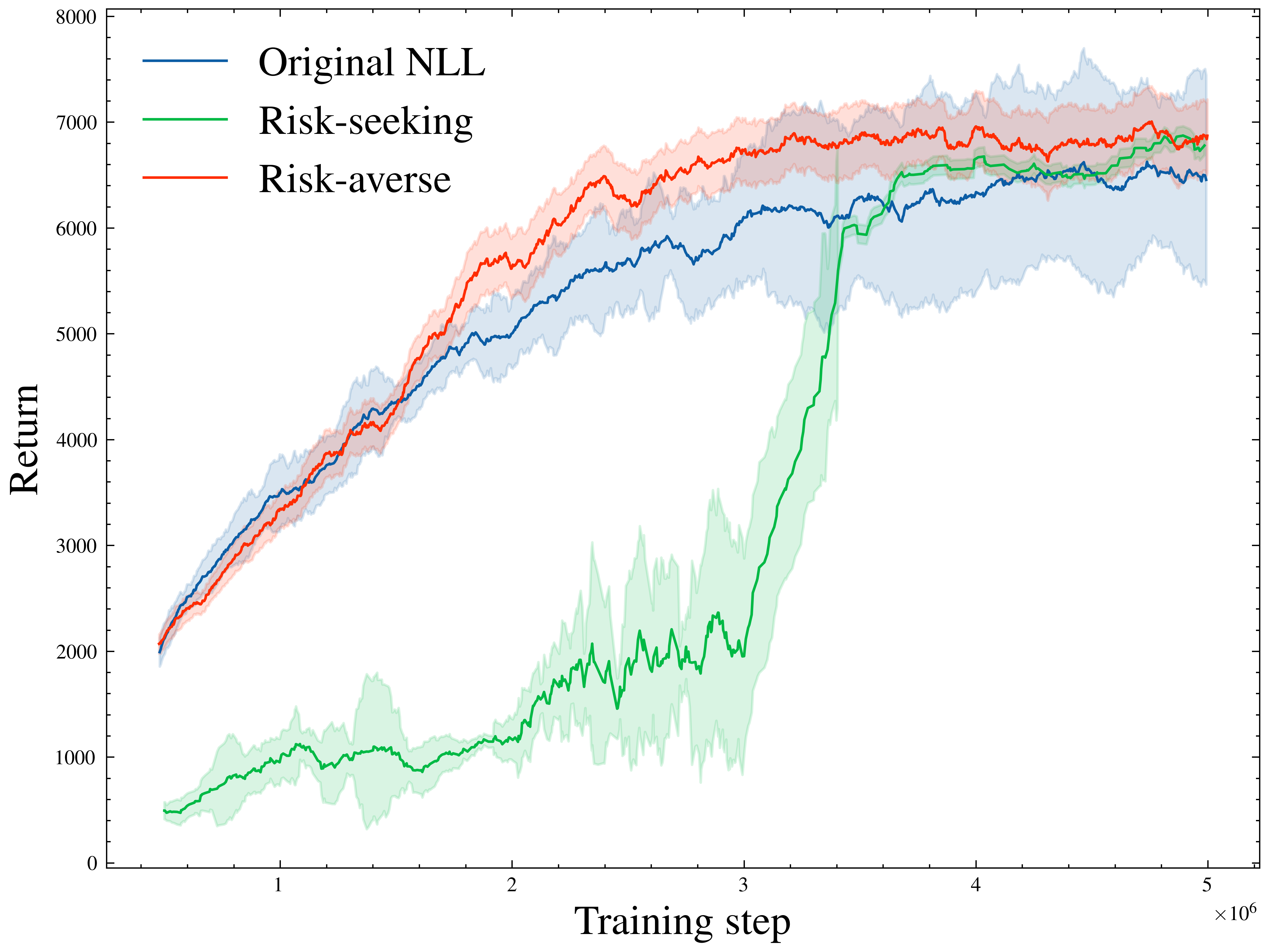
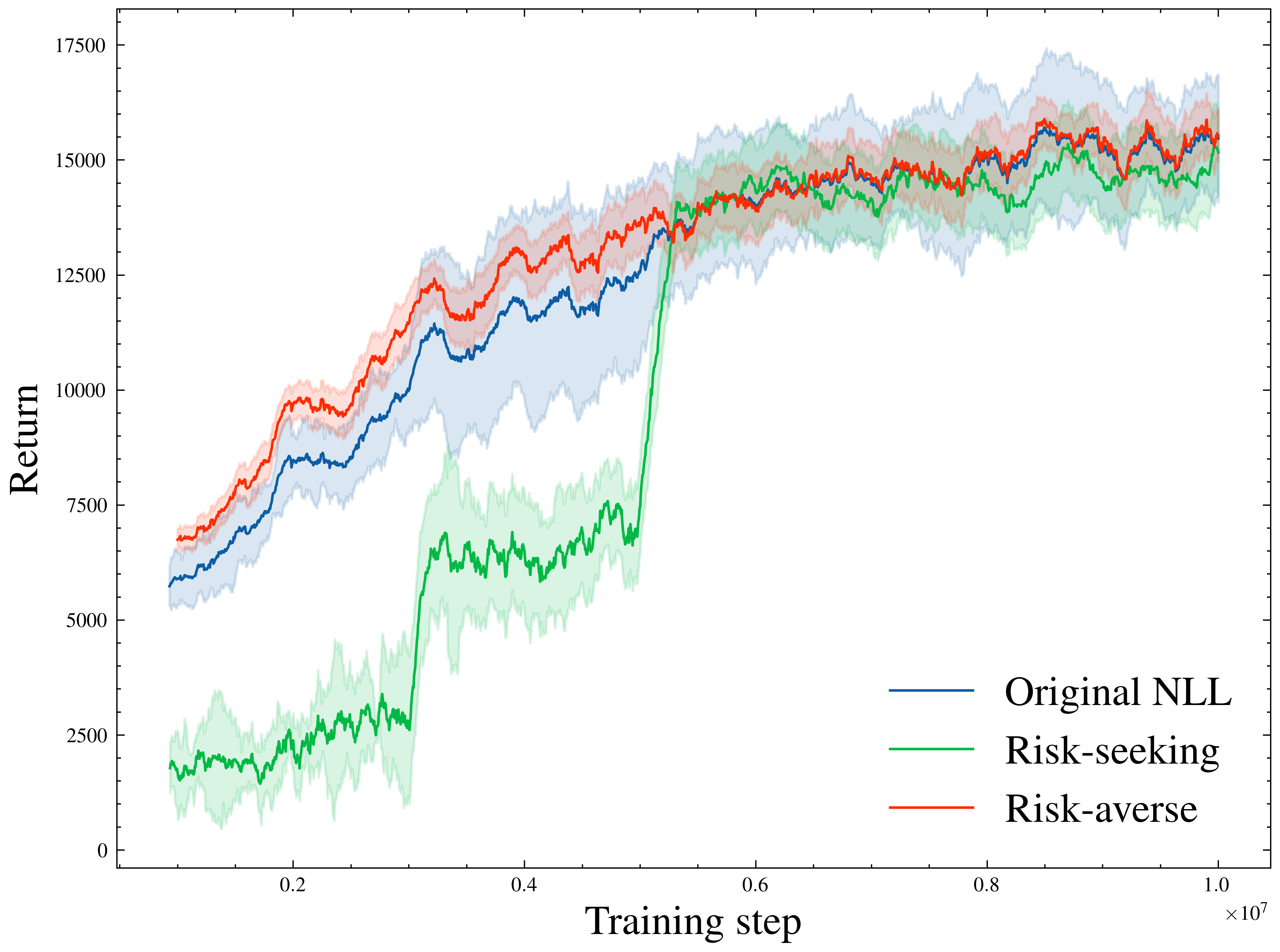
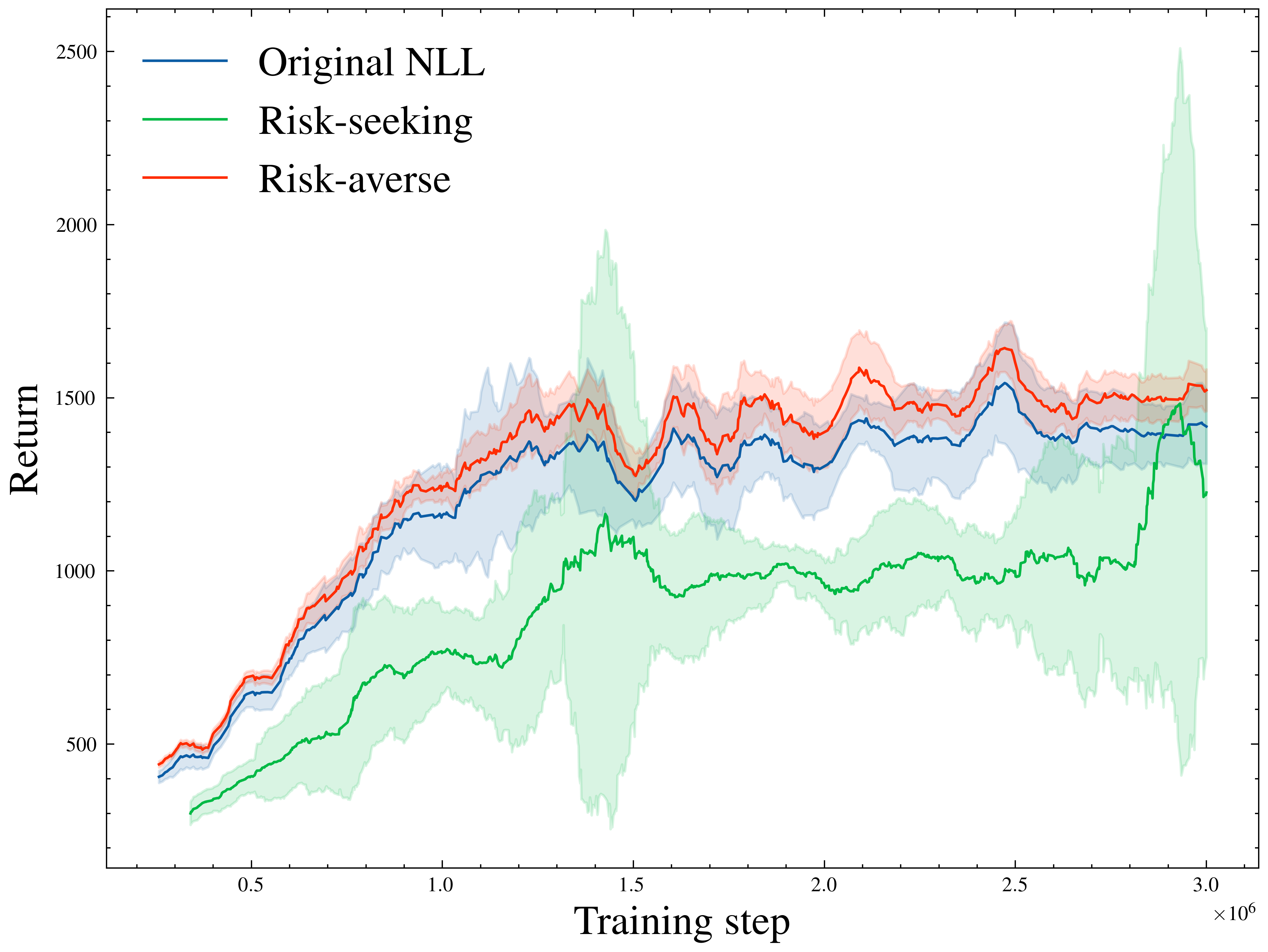
The theoretical foundation of the risk-averse weighting is provided by 2. Its empirical effectiveness, in comparison to the original GGD NLL and risk-seeking weighting , is demonstrated in Figure 11. It is evident that risk-aversion fosters sample-efficient training but does not necessarily translate to improved asymptotic performance. Notably, the adoption of risk-seeking behavior results in periodic performance jumps, indicating active exploration during side-stepping.
D.2 On BIEV regularization
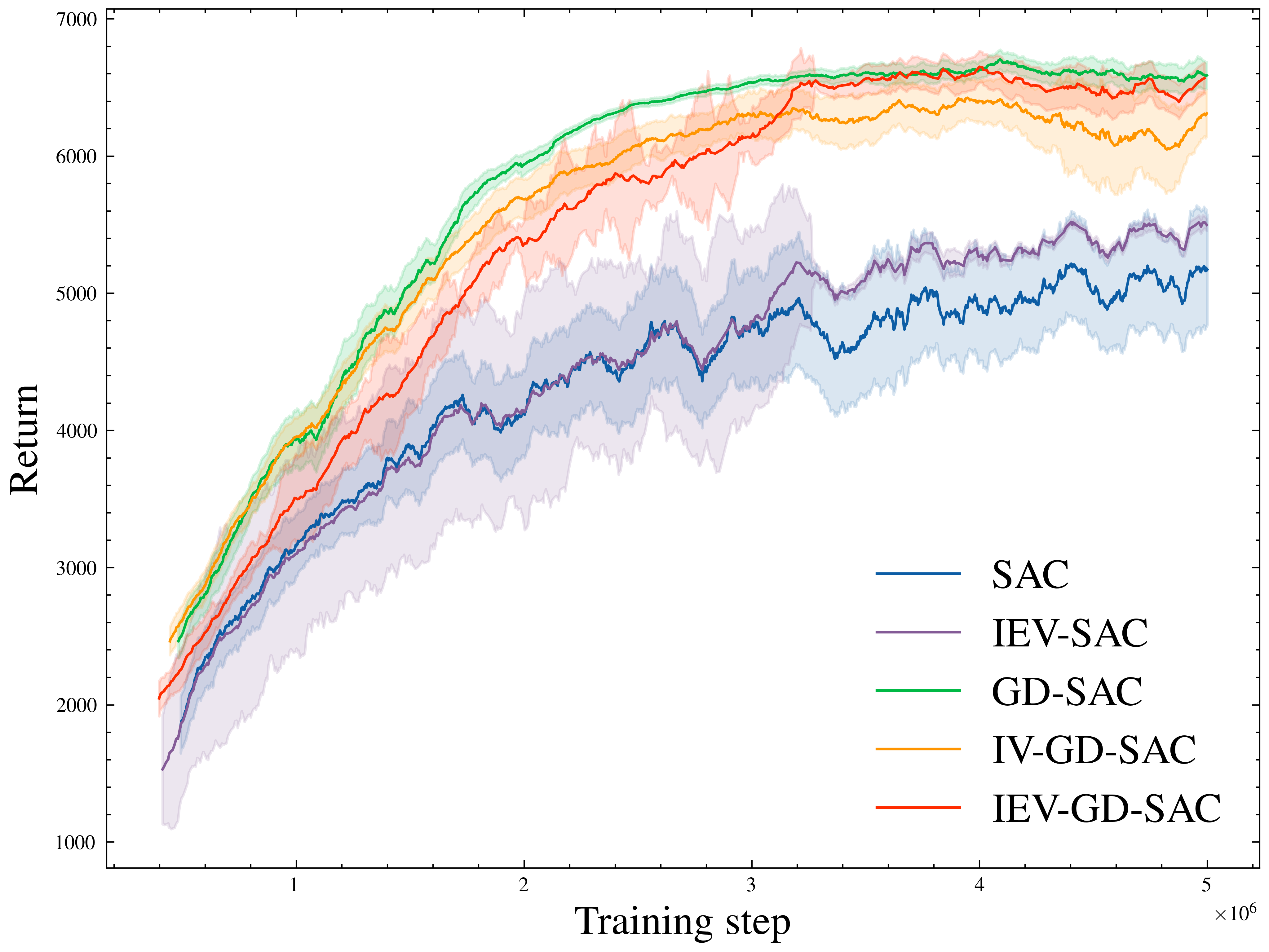
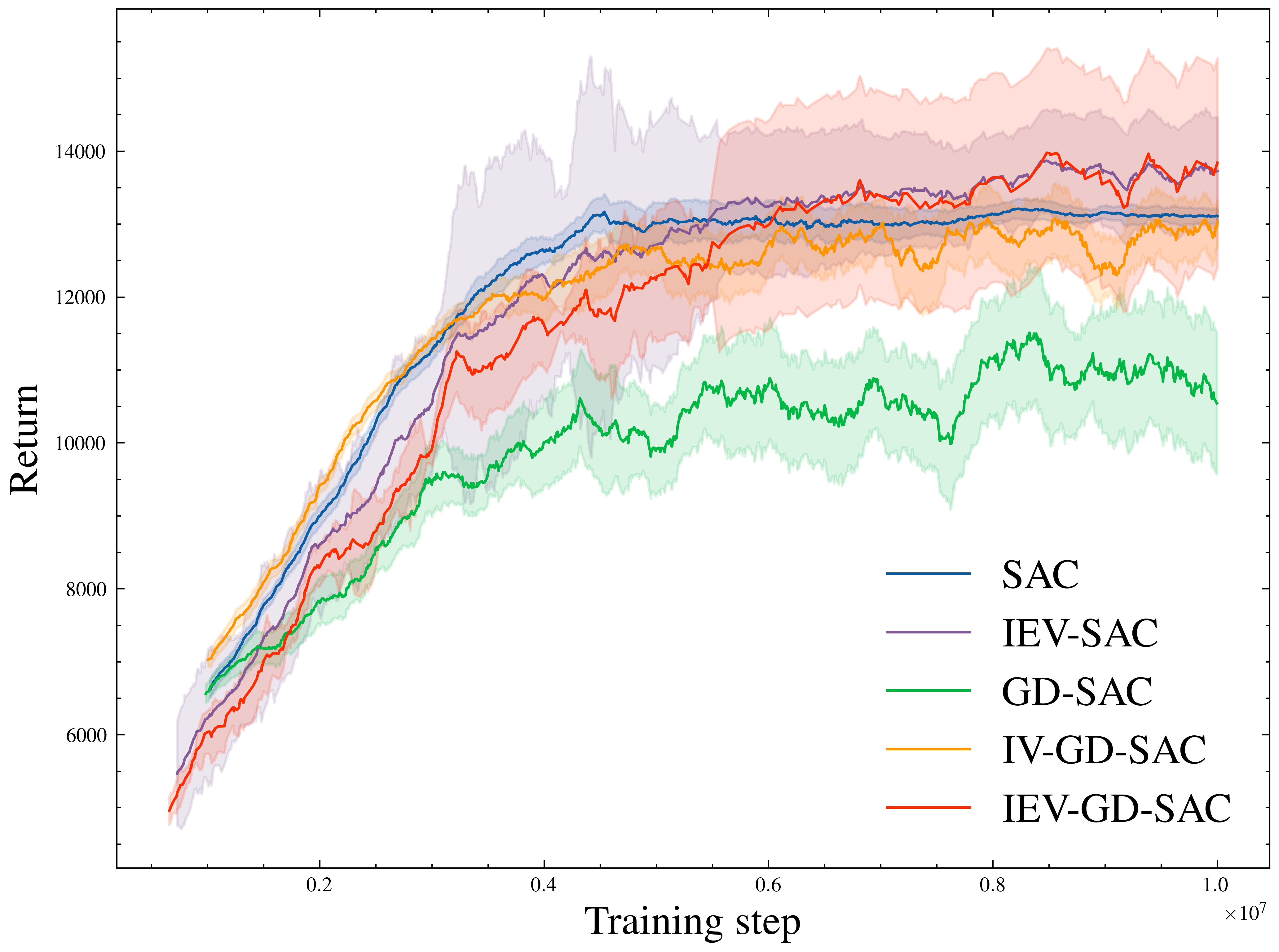
The BIEV loss term is inherently independent of the parameter head, as it relies solely on the variance of TD errors. This encourages us to investigate its efficacy independently of the GGD error modeling scheme. As depicted in Figure 12, the impact of BIEV on sample efficiency is nearly equivalent to that of BIV regularization, but slightly more advantageous in terms of asymptotic performance.
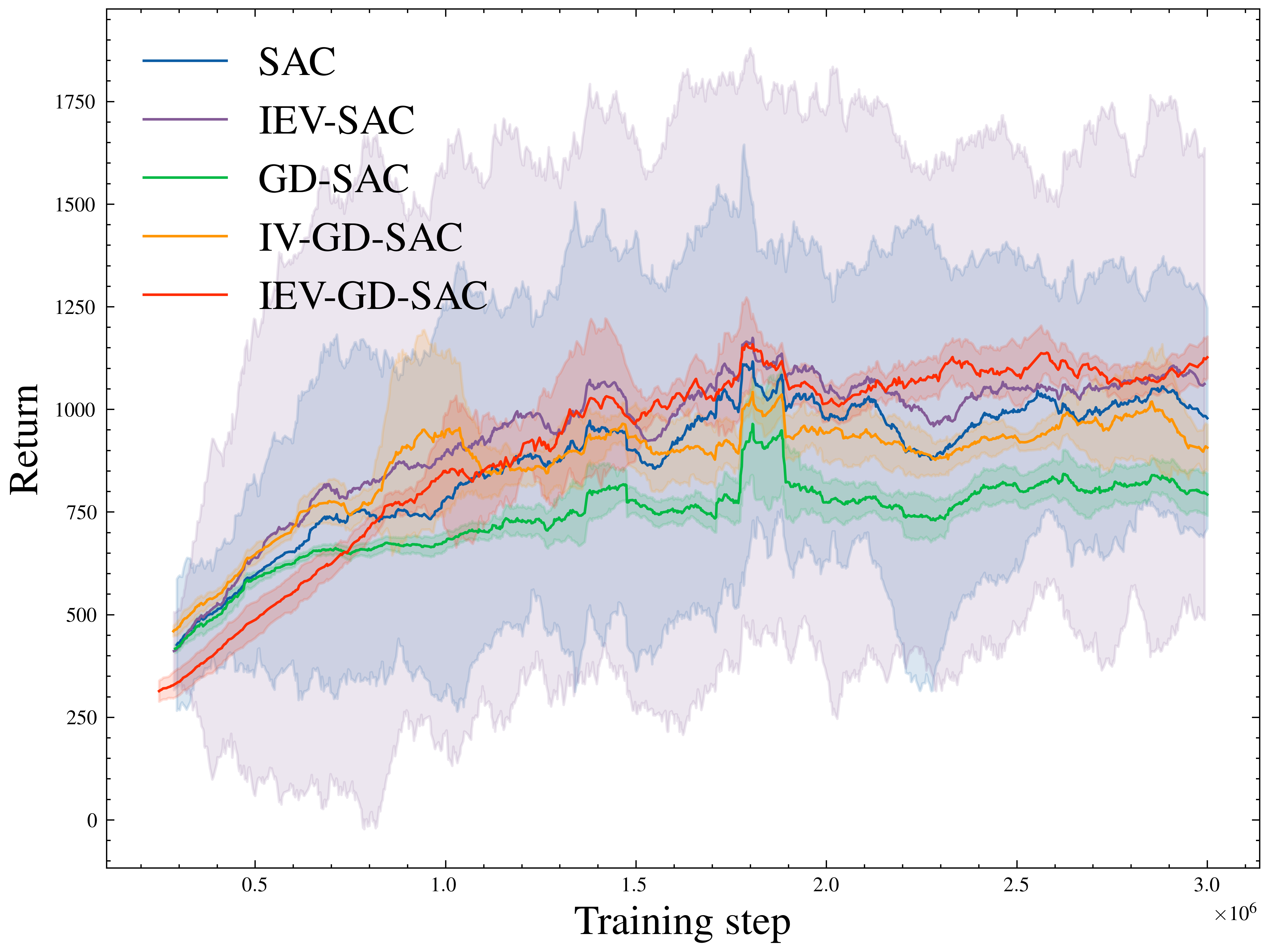
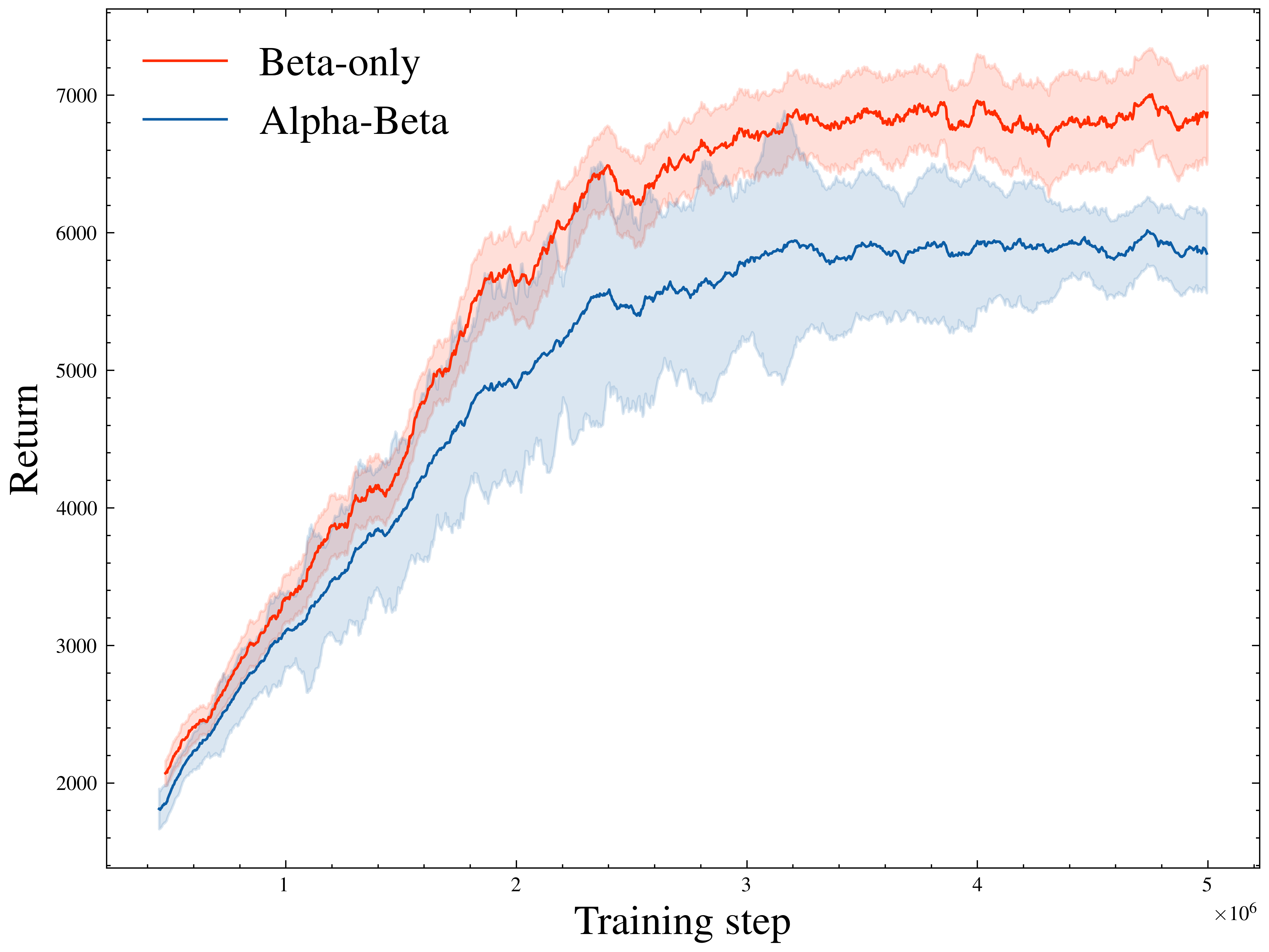
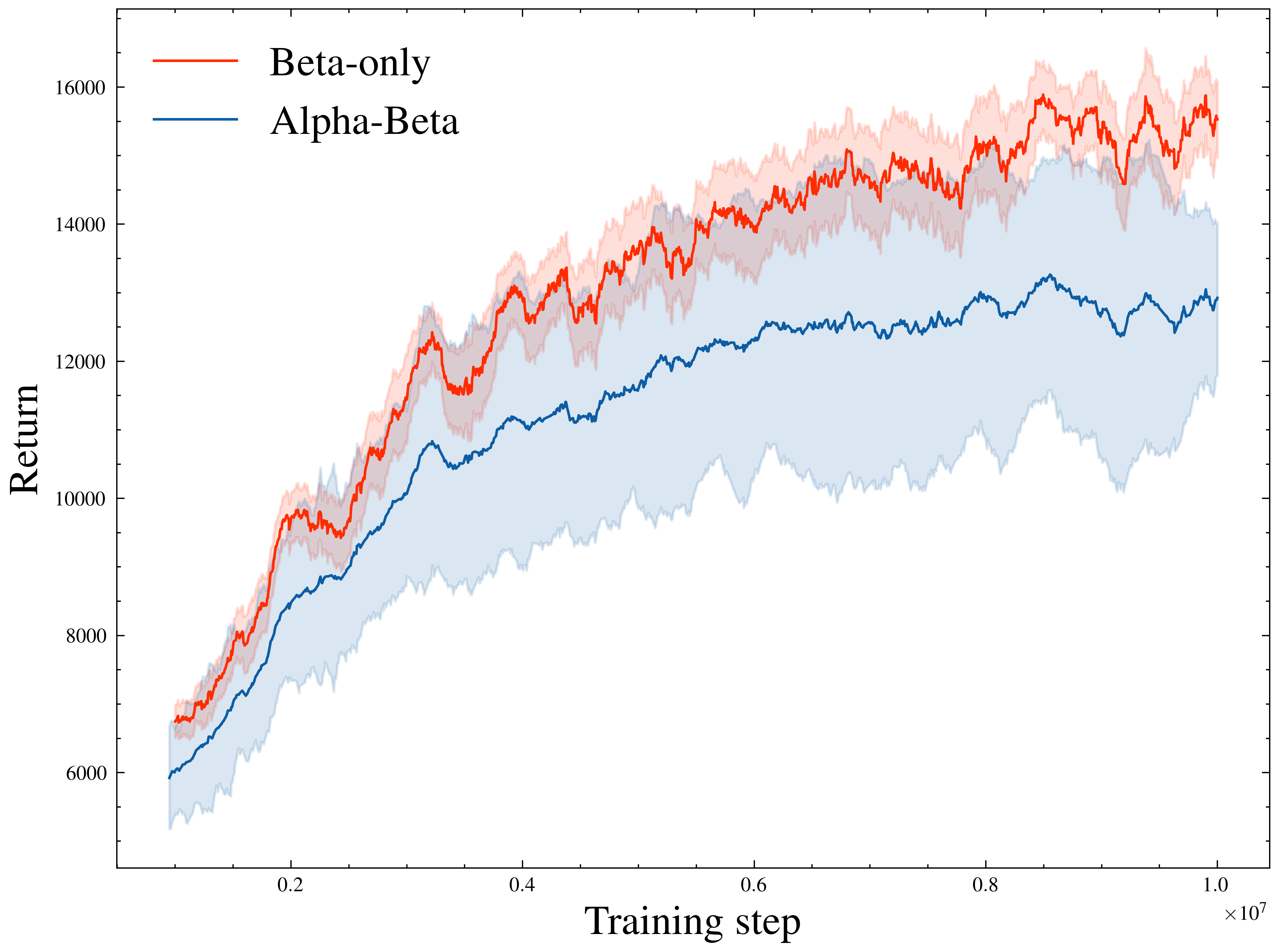
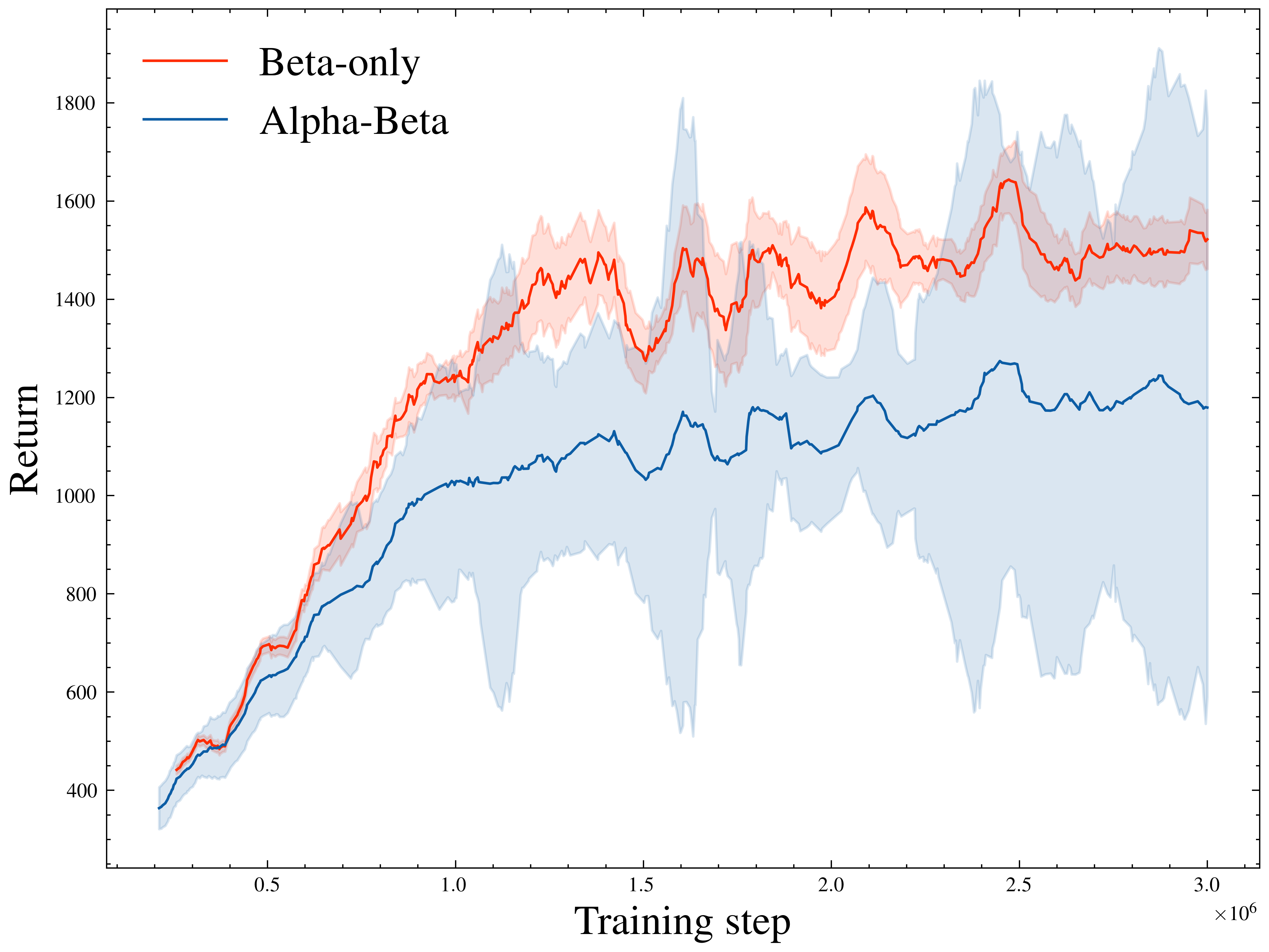
D.3 On alpha head
Appendix E Extension
As discussed in Section 5, we expand our empirical analysis to include -learning, with particular attention to DQN [43]. Figure 14 demonstrates that TD errors generated by DQN exhibit deviations from a Gaussian distribution and closely follow the GGD.
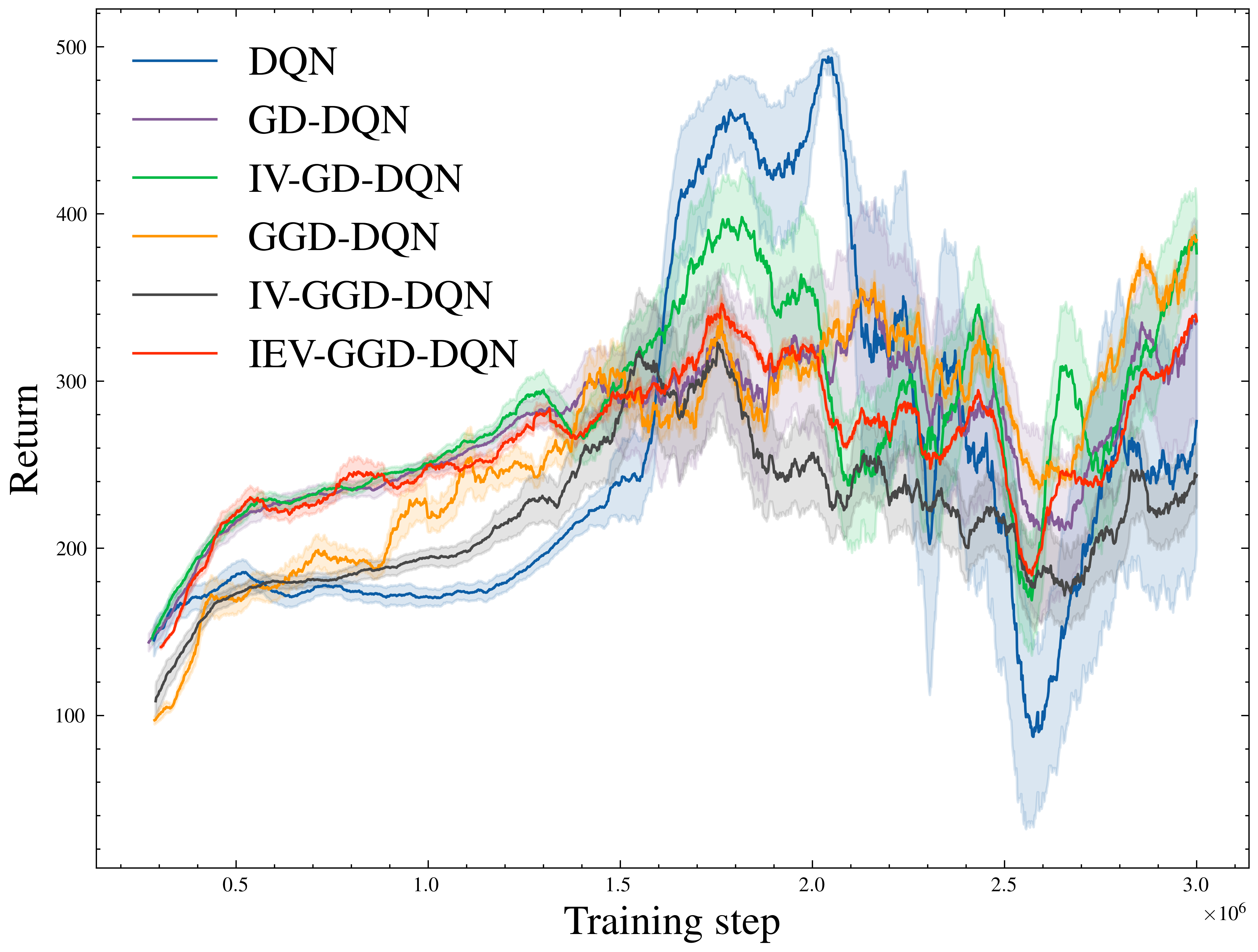
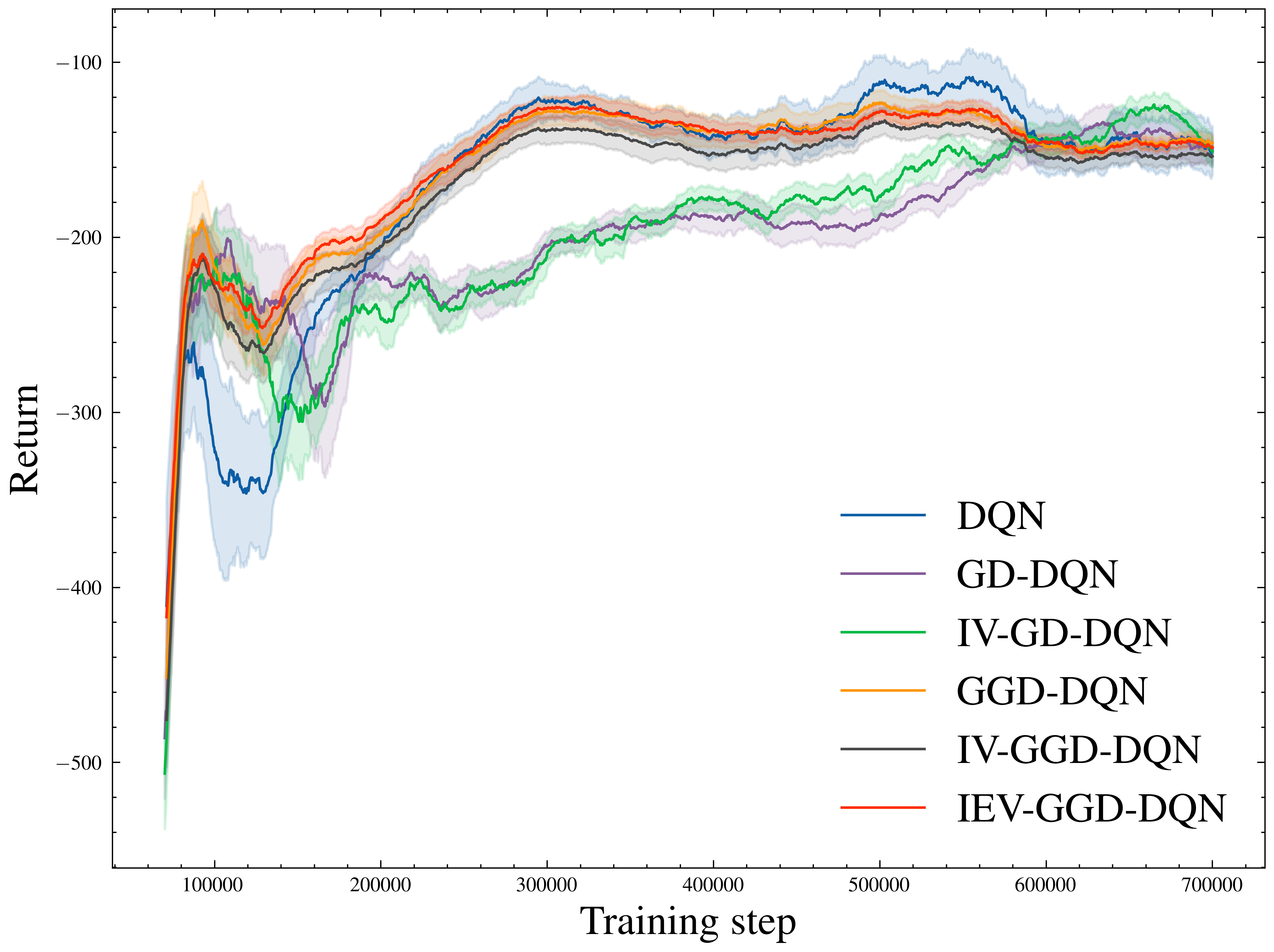
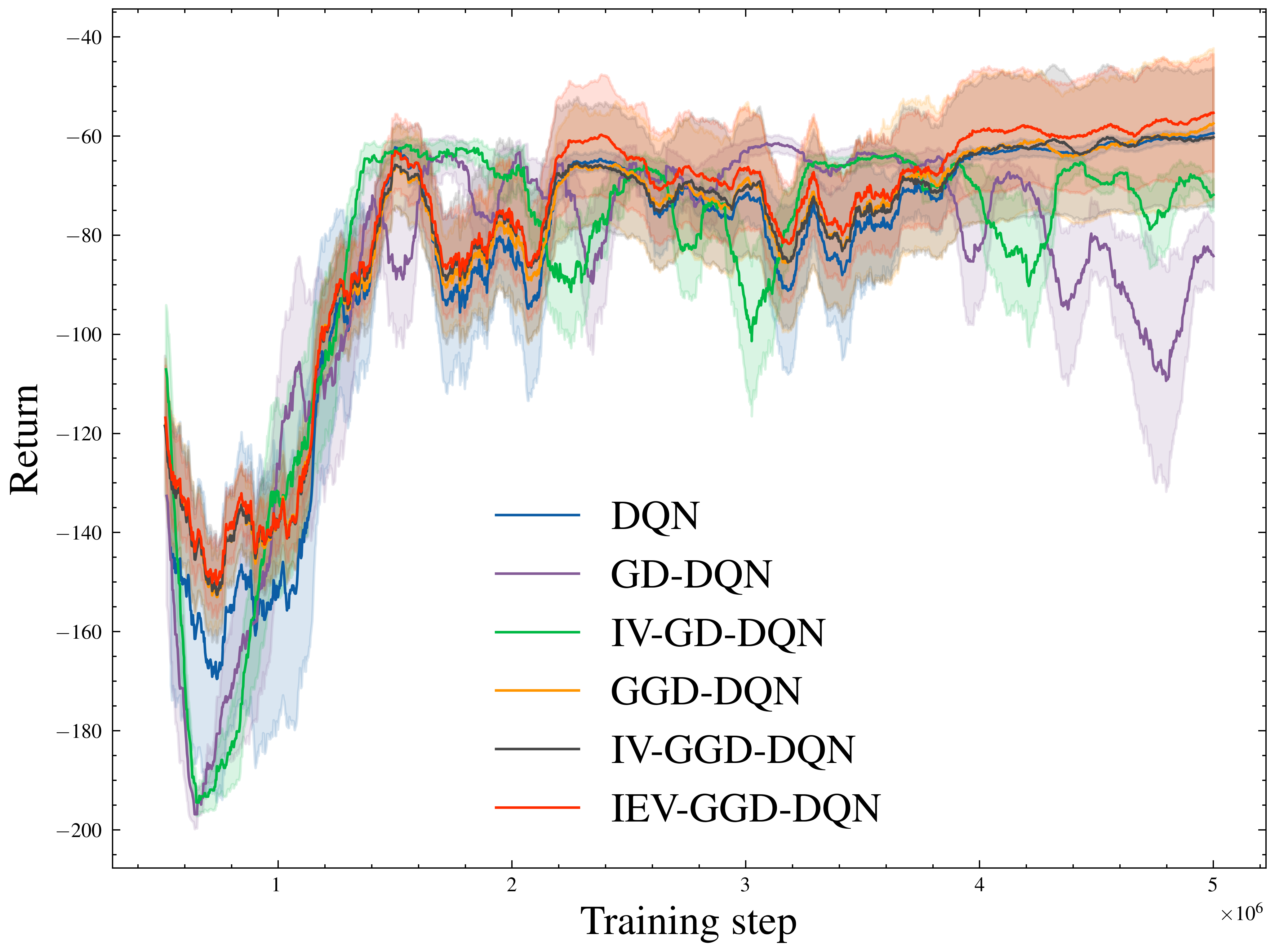
The performance of DQN in noisy discrete control environments, as depicted in Figure 15, highlights that simply applying our method to -learning is not sufficiently effective. Interestingly, regularization appears to have minimal impact, as evidenced by the similar performance observed among DQN variants equipped with GGD error modeling.
Since our implementation of DQN utilizes a greedy action policy, the approximated value function inherently represents the policy. Consequently, employing risk-averse weighting might impede exploration. Conversely, in policy gradient algorithms featuring separate policy networks, such risk-aversion serves to mitigate noisy supervision, aligning with its intended purpose. The adverse effects of risk-aversion are evident in Figure 16, where the model trained with the original NLL exhibits slightly superior sample efficiency compared to the proposed method.