Accelerated 3D Maxwell Integral Equation Solver using the Interpolated Factored Green Function Method

Abstract

This article presents an $\mathcal{O}(N\log N)$ method for numerical solution of Maxwell’s equations for dielectric scatterers using a 3D boundary integral equation (BIE) method. The underlying BIE method used is based on a hybrid Nyström-collocation method using Chebyshev polynomials. It is well known that such an approach produces a dense linear system, which requires $\mathcal{O}(N^{2})$ operations in each step of an iterative solver. In this work, we propose an approach using the recently introduced Interpolated Factored Green’s Function (IFGF) acceleration strategy to reduce the cost of each iteration to $\mathcal{O}(N\log N)$. To the best of our knowledge, this paper presents the first ever application of the IFGF method to fully-vectorial 3D Maxwell problems. The Chebyshev-based integral solver and IFGF method are first introduced, followed by the extension of the scalar IFGF to the vectorial Maxwell case. Several examples are presented verifying the $\mathcal{O}(N\log N)$ computational complexity of the approach, including scattering from spheres, complex CAD models, and nanophotonic waveguiding devices. In one particular example with more than 6 million unknowns, the accelerated IFGF solver runs 42x faster than the unaccelerated method.

I Introduction

Solution of Maxwell’s equations is quintessential to many modern applications including antennas, microwave and photonic devices. The lack of analytical solutions for general domains makes fast and accurate numerical solution methodology for Maxwell’s equations of utmost importance in such applications, in particular, for inverse design approaches, where accurate field and gradient information is needed in each iteration. The numerical methods available in the literature can largely be classified into the following three groups: finite-difference (FD) methods, finite-element (FE) methods, and integral equation (IE) methods. For this work, we have used a boundary integral equation (BIE) formulation due to its advantages for electromagnetic (EM) scattering problems over FD [9] and FE [10] methods, which are popular in the existing literature. In particular, BIE approaches only require discretizing the surfaces of domains unlike the finite-difference and the finite-element methods, which are volumetric in nature. In addition, BIE methods are almost dispersion-less due to analytically propagating information from sources to targets using Green’s functions, unlike FD and FE methods. A BIE approach was recently applied for designing and optimizing photonic devices [12, 13], demonstrating significant improvements in both runtime and accuracy.

The Method of Moments (MoM) approach is the most popular approach for discretizing BIEs in the available literature. The authors in the pioneering work [19] introduced the RWG basis functions in order to solve the electric field integral equation in conjunction with the MoM over flat triangular discretizations. A number of efforts have been made to alleviate some of the limitations arising from the first order basis functions and improve the performance, including using higher order basis functions (e.g., [20]) and phase-extracted basis functions (PEBFs) [26]. Other high-order approaches also have been introduced in the EM scattering context, such as [22], which produces a spectrally accurate approximation of the tangential surface current using a new set of tangential basis functions, as well as multiple other approaches as discussed in [21].

Recently, several works based on Nyström methods have been proposed [3][11][13][18][21]. In [3], the authors present a high-order method which decomposes the surface using non-overlapping curvilinear parametric patches, after which each patch is discretized using a Chebyshev grid in each parametric direction approximating the unknown density using Chebyshev polynomials. This work was extended to metallic and dielectric Maxwell scattering problems by leveraging the Magnetic Field Integral Equation (MFIE) and the N-Müller formulations of the electromagnetic problems, respectively, in [11]. The method was further accelerated by using GPU programming in [13] for the indirect N-Müller formulation and used to efficiently inverse design large 3D nanophotonic devices.

One of the main challenges of the Nyström method is that it produces dense linear systems leading to a $\mathcal{O}(N^{2})$ computational complexity for iterative solvers once the integral operator has been discretized. In order to reduce this computational cost various algorithmic acceleration strategies have been proposed [23] [24]. While these methods are effective in reducing the asymptotic computational cost, they all rely on the Fast Fourier Transform (FFT), which presents challenges for parallelization in the context of distributed memory parallel computer architectures. The recently introduced “Interpolated Factored Green’s Function” (IFGF) method [1], which relies on recursive interpolation by means of Chebyshev expansion of relatively low degrees, on the other hand, does not use the FFT and therefore is immune to this issue [25]. Note that due to the low degree approximations used, the IFGF method does not yield spectral accuracy.

We leverage the high-order Nyström method introduced in [3, 11] to discretize the integral operators and repurpose the IFGF method (initially demonstrated for the scalar Helmholtz case in [1]) to the 3D Maxwell scenario for accelerating the far interactions. To the best of our knowledge, this is the very first application of the IFGF method to 3D Maxwell electromagnetic scattering problems.

The rest of the paper is organized as follows: Section II briefly reviews the indirect N-Müller formulation. Section III presents the numerical methodology used for the approximation of the integral operators including the Chebyshev-based integral equation (CBIE) method [3, 11] used to decompose the surface and for approximating the singular integrals, and the IFGF algorithm [1] used to accelerate the far interactions. Section III also presents the necessary details for extending the IFGF algorithm to the full-vectorial 3D Maxwell scenario, including the application of the IFGF algorithm to evaluate the integral operators for multiple densities and computation of the corresponding normal derivative of the single layer operator. Finally, Section IV presents multiple numerical experiments that demonstrate the performance and accuracy of the proposed method. In particular, we observe a $\mathcal{O}(N\log N)$ complexity in our calculations, and a significant increase in speed in approximation of the operators. For instance, for a discretization containing more than 1.5 million points (more than 6 million unknowns), the computation time is reduced by a factor of $42$ for one forward map compared to the unaccelerated CBIE method. We conclude with a summary in Section V.

II Integral Equation Formulation

We consider the numerical approximation of the scattered electromagnetic fields, namely, the electric field ${\boldsymbol{E}}$ and the magnetic field ${\boldsymbol{H}}$ in a dielectric media in three dimensions. For simplicity, we consider two dielectric materials occupying the interior and exterior regions $\Omega_{i}$ and $\Omega_{e}$, respectively, of the surface $\Gamma$. The case for a composition of domains can be treated analogously [6]. The electromagnetic fields (${\boldsymbol{E}},{\boldsymbol{H}}$) and the material properties in the interior and the exterior regions are denoted using the subscripts $i$ and $e$, respectively, as illustrated in Fig. 1. Suppose we are given the incident field (${\boldsymbol{E}}^{\mathrm{inc}},{\boldsymbol{H}}^{\mathrm{inc}}$), and that the exterior unknown is the scattered field (${\boldsymbol{E}}^{\mathrm{sc}},{\boldsymbol{H}}^{\mathrm{sc}}$), where ${\boldsymbol{E}}_{e}={\boldsymbol{E}}^{\mathrm{inc}}+{\boldsymbol{E}}^{\mathrm{sc}}$ and ${\boldsymbol{H}}_{e}={\boldsymbol{H}}^{\mathrm{inc}}+{\boldsymbol{H}}^{\mathrm{sc}}$. Then the equations

$$\begin{cases}\nabla\times E_{i}-i\omega\mu_{i}H_{i}=0,\\ \nabla\times H_{i}+i\omega\epsilon_{i}E_{i}=0,\end{cases}\textrm{ in }\Omega_{i};$$ (1)

$$\begin{cases}\nabla\times E_{e}-i\omega\mu_{e}H_{e}=0,\\ \nabla\times H_{e}+i\omega\epsilon_{e}E_{e}=0,\end{cases}\textrm{ in }\Omega_{e};$$ (2)

and the transmission conditions

$$\begin{cases}{\boldsymbol{E}}_{i}\times{\boldsymbol{n}}=({\boldsymbol{E}}^{\mathrm{sc}}+{\boldsymbol{E}}^{\mathrm{inc}})\times{\boldsymbol{n}},\\ {\boldsymbol{H}}_{i}\times{\boldsymbol{n}}=({\boldsymbol{H}}^{\mathrm{sc}}+{\boldsymbol{H}}^{\mathrm{inc}})\times{\boldsymbol{n}},\end{cases}\mathrm{on}\;\Gamma,$$ (3)

are satisfied along with the Silver-Müller radiation condition.

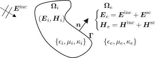
Figure 1: Illustration for EM scattering by dielectric medium.

An integral equation representation for the corresponding scattering problem can be found, for instance, in [5, Chap. 5], [6, Chap. 3] and [18]. As mentioned previously, we use a three-dimensional boundary integral representation to obtain the electromagnetic fields [4]. In particular, we consider the indirect N-Müller formulation [14]. To define the integral representation, let us define the tangential integrals

$$\boldsymbol{R}_{s}[\boldsymbol{\Phi}]({\boldsymbol{x}}) ={\boldsymbol{n}}\times\int_{\Gamma}G_{s}({\boldsymbol{x}},{\boldsymbol{x^{\prime}}})\boldsymbol{\Phi}({\boldsymbol{x^{\prime}}})d\gamma({\boldsymbol{x^{\prime}}}),$$ (4)

$$\boldsymbol{K}_{s}[\boldsymbol{\Phi}]({\boldsymbol{x}}) ={\boldsymbol{n}}\times\nabla\times\int_{\Gamma}G_{s}({\boldsymbol{x}},{\boldsymbol{x^{\prime}}})\boldsymbol{\Phi}({\boldsymbol{x^{\prime}}})d\gamma({\boldsymbol{x^{\prime}}}),$$ (5)

$$\boldsymbol{T}_{s}[\boldsymbol{\Phi}]({\boldsymbol{x}}) ={\boldsymbol{n}}\times\int_{\Gamma}\nabla G_{s}({\boldsymbol{x}},{\boldsymbol{x^{\prime}}})\mathrm{div}_{\Gamma}\boldsymbol{\Phi}({\boldsymbol{x^{\prime}}})d\gamma({\boldsymbol{x^{\prime}}})$$ (6)

where $s$ denotes the domain subscripts $e$ or $i$, and $G_{s}({\boldsymbol{x}},{\boldsymbol{x^{\prime}}})=\exp(i\kappa_{s}|{\boldsymbol{x}}-{\boldsymbol{x^{\prime}}}|)/(4\pi|{\boldsymbol{x}}-{\boldsymbol{x^{\prime}}}|)$ is the homogeneous space Green’s function of the Helmholtz equation. The indirect N-Müller integral formulation can then be written in matrix from as [13]

$$\begin{split}&\begin{bmatrix}\frac{(\mu_{e}+\mu_{i})}{2}\boldsymbol{I}+\boldsymbol{K}^{\Delta}_{\mu}&-(\boldsymbol{R}^{\Delta}+\boldsymbol{T}^{\Delta})\\ (\boldsymbol{R}^{\Delta}+\boldsymbol{T}^{\Delta})&\frac{(\epsilon_{e}+\epsilon_{i})}{2}\boldsymbol{I}+\boldsymbol{K}^{\Delta}_{\epsilon}\end{bmatrix}\begin{bmatrix}{\boldsymbol{m}}\\ {\boldsymbol{j}}\end{bmatrix}\\ &\quad\quad=\begin{bmatrix}\omega^{-1}\,{\boldsymbol{n}}\times{\boldsymbol{E}}^{\mathrm{inc}}\\ \omega^{-1}\,{\boldsymbol{n}}\times{\boldsymbol{H}}^{\mathrm{inc}}\end{bmatrix}\end{split}$$ (7)

where

$$\boldsymbol{K}^{\Delta}_{\alpha} \equiv(\alpha_{e}\boldsymbol{K}_{e}-\alpha_{i}\boldsymbol{K}_{i}),$$ (8)

$$\boldsymbol{R}^{\Delta} \equiv-i\omega(\mu_{e}\epsilon_{e}\boldsymbol{R}_{e}-\mu_{i}\epsilon_{i}\boldsymbol{R}_{i})\equiv\frac{-i}{\omega}(\kappa^{2}_{e}\boldsymbol{R}_{e}-\kappa^{2}_{i}\boldsymbol{R}_{i}),$$ (9)

$$\boldsymbol{T}^{\Delta} \equiv\frac{-i}{\omega}(\boldsymbol{T}_{e}-\boldsymbol{T}_{i}),$$ (10)

with $\boldsymbol{I}$ denoting the identity operator, and $\alpha$ denoting either $\epsilon$ and $\mu$ (see Remark 1).

Remark 1 (Weak singularity in (7))

The first two terms in the expansion of the exponential function in ($\nabla G_{e}-\nabla G_{i}$) vanish [7], thus the operators in (7) remain weakly singular.

III Numerical Methodology

As discussed in [17], the integral operators in (7) can be re-expressed via algebraic manipulation in terms of the weakly-singular operators of the form

$$S[\phi]({\boldsymbol{x}})=\int_{\Gamma}G_{\kappa}({\boldsymbol{x}},{\boldsymbol{x^{\prime}}})\phi(y)d\gamma({\boldsymbol{x^{\prime}}}),$$ (11)

and the normal derivative

$$D[\phi]({\boldsymbol{x}})=\frac{\partial S[\phi]({\boldsymbol{x}})}{\partial n({\boldsymbol{x}})},$$ (12)

where $\phi$ represents a Cartesian component of one of the surface current densities ${\boldsymbol{j}}=(j_{x},j_{y},j_{z})$ and ${\boldsymbol{m}}=(m_{x},m_{y},m_{z})$; or one of the surface divergences $\mathrm{div}_{\Gamma}{\boldsymbol{j}}$ and $\mathrm{div}_{\Gamma}{\boldsymbol{m}}$ of the current densities. Note that for the surface divergences $\mathrm{div}_{\Gamma}{\boldsymbol{j}}$ and $\mathrm{div}_{\Gamma}{\boldsymbol{m}}$, only the operator $S[\phi]$ needs to be computed. The EM operators are then evaluated by further compositions of other operators such as gradient as per the definitions of the operators (8)-(10) involved in (7). The required derivatives are obtained using the Chebyshev recurrence relations [15] based on the underlying Chebyshev grids given by (16) below. To approximate the above integrals and to further obtain accurate values of the EM operators, the proposed IFGF accelerated Chebyshev-based (CBIE-IFGF) method discretizes the surface $\Gamma$ as described in what follows.

III-A CBIE-IFGF: Surface Discretization.

The proposed CBIE-IFGF method decomposes the surface $\Gamma$ into a set of $P$ non-overlapping, curvilinear quadrilateral patches $\Gamma_{p};p=0,\dots,(P-1)$ such that

$$\Gamma=\bigcup_{p=0}^{P-1}\Gamma_{p},$$ (13)

where each patch $\Gamma_{p}$ has a parametrization $\boldsymbol{\eta}_{p}(u,v)$ with $(u,v)\in[-1,1]^{2}$, as illustrated Fig. 2.

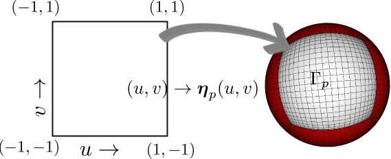
Figure 2: Mapping the square $[-1,1]\times[-1,1]$ in parametric $(u,v)$-space to a patch on the surface of a sphere in Cartesian coordinates.

Following (11) and (13), we can write

$$S[\phi]({\boldsymbol{x}})=\sum_{p=0}^{P-1}S_{p}({\boldsymbol{x}}),$$ (14)

where

$$S_{p}({\boldsymbol{x}})=\!\int\limits_{[-1,1]^{2}}\!\!\!G_{\kappa}({\boldsymbol{x}},\boldsymbol{\eta}_{p}(u,v))\phi_{p}(u,v)J_{p}(u,v)dudv,$$ (15)

$G_{p}({\boldsymbol{x}},u,v)=G({\boldsymbol{x}},\boldsymbol{\eta}_{p}(u,v))$, $\phi_{p}(u,v)=$ $\phi(\boldsymbol{\eta}_{p}(u,v))$, and $J_{p}(u,v)$ denotes the Jacobian of the parametrization $\boldsymbol{\eta}_{p}$.

In each of the patches, the method places an open Chebyshev grid along $u$ and $v$ directions:

$$u_{i}=\cos((k+0.5)\pi/N_{C}):k=0,\dots,N_{C}-1,$$ (16)

(similarly, for $v$) for certain integer value of $N_{C}$. (For simplicity of the description, we have used the same number of points in both parametric directions—which is not a necessity.) The collection $\Gamma_{N}$ of the discretization points on $\Gamma$ is given below:

$$\Gamma_{N}=\left\{\right.{\boldsymbol{x}}_{\ell}= \left.\boldsymbol{\eta}_{p}(u_{i},v_{j}):\ell=j+N_{C}i+pN^{2}_{C};\right.$$

$$\left.0\leq i,j\leq N_{C}-1;0\leq p\leq P-1\right\}.$$ (17)

The total number of discretization points are $N=P\times N_{C}^{2}$. The resulting linear system that arises upon discretizing (7) based on the discretization $\Gamma_{N}$ of the surface $\Gamma$ is denoted by

$$A\boldsymbol{y}=b,$$ (18)

where the matrix $A$ is of size $4N\times 4N$. The proposed method uses GMRES to solve the linear system in (18). Next, we discuss the approximation methodology for the integral $S_{p}({\boldsymbol{x}})$ over a patch $\Gamma_{p}$ for $p=0,\dots,P-1$ for a given target point ${\boldsymbol{x}}$.

III-B Approximating the Integral $S_{p}({\boldsymbol{x}})$ for $p=0,\dots,P-1$.

There are two main difficulties in approximating $S_{p}({\boldsymbol{x}})$ (15) for $p=0,\dots,P-1$: first, the singular and near-singular behavior of the kernel when the target point ${\boldsymbol{x}}$ and the source point ${\boldsymbol{x^{\prime}}}=\boldsymbol{\eta}_{p}(u,v)$ coincide or, are in close proximity; and second, the $\mathcal{O}(N^{2})$ cost required to evaluate the discrete integrator for the regular/non-singular case when the source and the target points are sufficiently away from each other.

In order to classify the singular and non-singular target/observation points for integration over a given surface patch $\Gamma_{p}$, we define the following “distance of a point ${\boldsymbol{x}}$ from a surface patch $\Gamma_{p}$”:

$$\mathrm{dist}({\boldsymbol{x}},\Gamma_{p})=\inf\{|{\boldsymbol{x}}-{\boldsymbol{x^{\prime}}}|:{\boldsymbol{x^{\prime}}}\in\Gamma_{p}\}.$$ (19)

Moreover, for a certain number $\delta>0$, let us define the index sets $\mathscr{S}_{\ell}$ and $\mathscr{R}_{\ell}$ for a point ${\boldsymbol{x}}_{\ell}$

$$\mathscr{S}_{\ell} \coloneq\{p:\mathrm{dist}({\boldsymbol{x}}_{\ell},\Gamma_{p})\leq\delta\},~{}\mathrm{and}$$ (20)

$$\mathscr{R}_{\ell} \coloneq\{p:\mathrm{dist}({\boldsymbol{x}}_{\ell},\Gamma_{p})>\delta\}$$ (21)

containing the indices of the patches $\Gamma_{p}$ $(p=0,\dots,P-1)$ for which the point ${\boldsymbol{x}}_{\ell}$ is treated as a singular, or near-singular and a regular/non-singular point, respectively. Thus

$$S[\phi]({\boldsymbol{x}}_{\ell})=\sum_{p\in\mathscr{S}_{\ell}}S_{p}({\boldsymbol{x}}_{\ell})+\sum_{p\in\mathscr{R}_{\ell}}S_{p}({\boldsymbol{x}}_{\ell}).$$ (22)

We start our discussion on the quadrature to approximate $S_{p}({\boldsymbol{x}}_{\ell})$ for the non-singular case ($p\in\mathscr{R}_{\ell}$) and the singular case ($p\in\mathscr{S}_{\ell}$) in Section III-C and Section III-D, respectively, in what follows.

III-C Approximation of $S_{p}({\boldsymbol{x}}_{\ell})$: Non-Singular Case.

The non-singular case can be treated using Fejér quadrature based on the nodes given by (16) and the weights

$$w_{n}=\frac{2}{N_{C}}\left[1-2\sum\limits_{m=1}^{\lfloor{N_{C}/2}\rfloor}\frac{1}{4m^{2}-1}\cos\left(\frac{m\pi(2n+1)}{N_{C}}\right)\right],$$ (23)

for $n=0,\dots,N_{C}-1$. A straightforward application of the Fejér quadrature at ${\boldsymbol{x}}_{\ell}$ reads

$$\mathcal{S}_{p}({\boldsymbol{x}}_{\ell})\approx\sum\limits_{i=0}^{N_{C}-1}\sum\limits_{j=0}^{N_{C}-1}G({\boldsymbol{x}}_{\ell},u_{i},v_{j})\phi_{p}(u_{i},v_{j})J_{p}(u,v)w_{i}w_{j}.$$ (24)

Clearly, such an application of the Fejér quadrature has an overall complexity of $\mathcal{O}(N^{2})$; in order to get a reduced $\mathcal{O}(N\log N)$ run time in the non-singular calculation, it is accelerated using the IFGF algorithm discussed in Section III-E.

III-D Approximation of $S_{p}({\boldsymbol{x}}_{\ell})$: Singular Case.

The evaluation of $S_{p}({\boldsymbol{x}}_{\ell})$ for the singular case requires special treatment via change of variable to resolve the singularity present in the kernel. Given that this change of variable as such depends on the target point, in order to make the singular calculation more efficient, the method uses precomputed integral moments of the product of the kernel and the Chebyshev functions of the parametric variables $u$ and $v$, along with the Jacobian of the parametric change of variable. Letting the Chebyshev expansion of the density $\phi_{p}(u,v)$:

$$\phi_{p}(u,v)\approx\displaystyle\sum\limits_{m=0}^{N_{C}-1}\sum_{n=0}^{N_{C}-1}\!\!a^{p}_{m,n}T_{m}(u)T_{n}(v)$$ (25)

based on the nodes (16); using (15) the integral $S_{p}({\boldsymbol{x}})$ can be approximated by evaluating the summation

$$S_{p}({\boldsymbol{x}}_{\ell})\approx\displaystyle\sum\limits_{m=0}^{N_{C}-1}\sum_{n=0}^{N_{C}-1}a^{p}_{m,n}\beta^{p,\ell}_{m,n},$$

where the moments have been computed as

$$\beta^{p,\ell}_{m,n}=\displaystyle\int\limits_{[-1,1]^{2}}G({\boldsymbol{x}}_{\ell},u,v)T_{m}(u)T_{n}(v)J_{p}(u,v)dudv.$$ (26)

To evaluate the moments (26) at a target point ${\boldsymbol{x}}_{\ell}\in\Gamma_{N}$, the method finds the point ${\boldsymbol{x}}_{\ell}^{p}={\boldsymbol{x}}_{p}(u^{p}_{\ell},v^{p}_{\ell})\in\Gamma_{p}$ that is closest to ${\boldsymbol{x}}_{\ell}$, or rather its parametric-space coordinates, which in general can be found as the solution of the distance minimization problem

$$(\tilde{u}^{p}_{\ell},\tilde{v}^{p}_{\ell})=\underset{(u,v)\in[-1,1]^{2}}{\mathrm{arg\,min}}|{\boldsymbol{x}}_{\ell}-\boldsymbol{\eta}_{p}(u,v)|.$$ (27)

Following [3], the method utilizes the golden section search algorithm, with initial bounds obtained from a direct minimization over all of the original discretization points in $\Gamma_{p}$. Note that if ${\boldsymbol{x}}_{\ell}$ is itself a grid point in $\Gamma_{p}$ and ${\boldsymbol{x}}_{\ell}=\boldsymbol{\eta}_{p}(u_{m},v_{n})$ then the parametric coordinates $(\tilde{u}^{p}_{\ell},\tilde{v}^{p}_{\ell})=(u_{m},v_{n})$.

The method utilizes a one-dimensional change of variable to each coordinate in the $uv$-space to construct a clustered grid around a given target point. To this end, we consider the following mapping $w:[0,2\pi]\rightarrow[0,2\pi]$, with parameter $d\geq 2$ (see, [4, Section 3.5]):

$$w(\tau)=2\pi\frac{[\nu(\tau)^{d}]}{[v(\tau)]^{d}+[\nu(2\pi-\tau)]^{d}},\;0\leq\tau\leq 2\pi,$$ (28)

where

$$v(\tau)=\left(\frac{1}{d}-\frac{1}{2}\right)\left(\frac{\pi-\tau}{\pi}\right)^{3}+\frac{1}{d}\left(\frac{\tau-\pi}{\pi}\right)+\frac{1}{2}.$$ (29)

It can be shown that $w$ has vanishing derivatives up to order $d-1$ at the interval endpoints.

Further, the one-dimensional change of variables (defined on the basis of the change of variable above)

$$\xi_{\alpha}(\tau)=\begin{cases}\alpha+\left(\frac{\mathrm{sgn}(\tau)-\alpha}{\pi}\right)w(\pi|\tau|),\;\mathrm{for}\;\alpha\neq\pm 1,\\ \alpha-\left(\frac{1+\alpha}{\pi}\right)w(\pi|\frac{\tau-1}{2}|),\;\mathrm{for}\;\alpha=1,\\ \alpha+\left(\frac{1-\alpha}{\pi}\right)w(\pi|\frac{\tau+1}{2}|),\;\mathrm{for}\;\alpha=-1\end{cases}$$ (30)

clusters the points around $\alpha$. Indeed, a use of Fejér’s rule with $N_{\beta}$ points yields

$$\beta^{p,\ell}_{m,n}\approx\displaystyle\sum\limits_{i=0}^{N_{\beta}-1}\sum\limits_{j=0}^{N_{\beta}-1}\!\! \!\!G({\boldsymbol{x}}_{\ell},u_{i}^{p,\ell},v_{j}^{p,\ell})J_{p}(u_{i}^{p,\ell},v_{j}^{p,\ell})T_{m}(u_{i}^{p,\ell})$$ (31)

$$T_{n}(v_{j}^{p,\ell})\mu_{i}^{u,p,\ell}\mu_{j}^{v,p,\ell}w_{i}w_{j}$$

where

$$u_{i}^{p,\ell}=\xi_{\tilde{u}_{\ell}^{p}}(t_{i}), v_{j}^{p,\ell}=\xi_{\tilde{v}_{\ell}^{p}}(t_{j}),$$ (32)

$$\mu_{i}^{u,p,\ell}=\frac{d\xi_{\tilde{u}_{\ell}^{p}}}{d\tau}(t_{i}), \mu_{j}^{v,p,\ell}=\frac{d\xi_{\tilde{v}_{\ell}^{p}}}{d\tau}(t_{j}),$$ (33)

for $i,j=0,\dots,N^{\beta}-1$. These integral moments (and the required closest points) are computed only once at the beginning of each run. The value of $N_{\beta}$ is chosen (based on the experiments presented in [11, Fig. 3a-3b and TABLE II]) to match the accuracy provided by the IFGF interpolation algorithm, which we describe in the following subsection.

III-E IFGF Acceleration of Non-singular Calculation.

As discussed in Section III-C, for a given surface discretization $\Gamma_{N}:=\{x_{1},\dots,x_{N}\}$, we need to evaluate a discrete sum of the form

$$I(x_{\ell}):=\sum_{\begin{subarray}{c}m=1\\ m\neq\ell\end{subarray}}^{N}a_{m}G({\boldsymbol{x}}_{\ell},{\boldsymbol{x}}_{m}),\quad\ell=1,\dots,N$$ (34)

where $N$ denotes a given positive integer, $m=1,\dots,N,$ and, ${\boldsymbol{x}}_{m}\in\Gamma_{N}$ and $a_{m}\in\mathbb{C}$ denote pairwise different points and given complex numbers, respectively (cf. (22) for $p\in\mathscr{R}_{\ell}$ and (24)). Clearly, a direct evaluation of the sum $I(x)$ for all $x\in\Gamma_{N}$ requires $\mathcal{O}(N^{2})$ operations. The recursive interpolation based IFGF approach, introduced in [1], can reduce the cost of this evaluation to $\mathcal{O}(N\log N)$. We first describe the IFGF interpolation strategy for a scalar density $\phi$, and for the contribution coming from the source points within a certain box in what follows.

III-F IFGF Interpolation: Single Source Box.

Consider the axis aligned box $B({\boldsymbol{x}}^{S},H)$

$$B \left({\boldsymbol{x}}^{S},H\right):=\left[({\boldsymbol{x}}_{S})_{1}-\frac{H}{2},({\boldsymbol{x}}_{S})_{1}+\frac{H}{2}\right)\times$$

$$\left[({\boldsymbol{x}}_{S})_{2}-\frac{H}{2},({\boldsymbol{x}}_{S})_{2}+\frac{H}{2}\right)\times\left[({\boldsymbol{x}}_{S})_{3}-\frac{H}{2},({\boldsymbol{x}}_{S})_{3}+\frac{H}{2}\right)$$

in $\mathbb{R}^{3}$ of side length $H>0$ and centered at $x^{S}=((x_{S})_{1},(x_{S})_{2},(x_{S})_{3})\in\mathbb{R}^{3}$. Let $\Gamma^{S}_{N_{S}}:=\{x_{1}^{S},\dots,x_{N_{S}}^{S}\}\in B(x^{S},H)\cap\Gamma_{N}$ denote the source points contained in $B(x^{S},H)$. Then, the contribution of the source points within the box $B(x^{S},H)$ at a target point ${\boldsymbol{x}}_{\ell}^{T}$ is given by

$$I_{S}({\boldsymbol{x}}_{\ell}^{T}):=\displaystyle\sum_{m=1}^{N_{S}}a_{m}^{S}G({\boldsymbol{x}}_{\ell}^{T},{\boldsymbol{x}}_{m}^{S}),\quad\ell=1,\dots,N_{T}.$$ (35)

To efficiently evaluate the sum $I_{S}({\boldsymbol{x}})$, the IFGF method first factorizes the kernel as

$$G({\boldsymbol{x}},{\boldsymbol{x^{\prime}}})=G({\boldsymbol{x}},{\boldsymbol{x}}^{S})g_{S}({\boldsymbol{x}},{\boldsymbol{x^{\prime}}})$$ (36)

where $G({\boldsymbol{x}},{\boldsymbol{x}}^{S})=\frac{e^{i\kappa|{\boldsymbol{x}}-{\boldsymbol{x}}^{S}|}}{4\pi|{\boldsymbol{x}}-{\boldsymbol{x}}^{S}|}$ is called the “centered factor”, and

$$g_{S}({\boldsymbol{x}},{\boldsymbol{x^{\prime}}}) =\frac{|{\boldsymbol{x}}-{\boldsymbol{x}}^{S}|}{|{\boldsymbol{x}}-{\boldsymbol{x^{\prime}}}|}e^{i\kappa(|{\boldsymbol{x}}-{\boldsymbol{x^{\prime}}}|-|{\boldsymbol{x}}-{\boldsymbol{x}}^{S}|)}$$ (37)

is called the “analytic factor”. Using the factorization (36), we can write (35) as

$$I_{S}({\boldsymbol{x}}_{\ell}^{T})=\displaystyle\sum_{m=1}^{N_{S}}a_{m}^{S}G({\boldsymbol{x}}_{\ell}^{T},{\boldsymbol{x}}_{m}^{S})=G({\boldsymbol{x}}_{\ell}^{T},{\boldsymbol{x}}_{S})F_{S}({\boldsymbol{x}}_{\ell}^{T})$$ (38)

where

$$F_{S}({\boldsymbol{x}}_{\ell}^{T})=\displaystyle\sum_{m=1}^{N_{S}}a_{m}^{S}g_{S}({\boldsymbol{x}}_{\ell}^{T},{\boldsymbol{x}}_{m}^{S})$$ (39)

is the analytic factor contribution.

Defining the radius of the source box $B({\boldsymbol{x}}^{S},H)$ by $h:=\frac{\sqrt{3}}{2}H$, and the variable $s:=h/r$ where $r:=|{\boldsymbol{x}}-{\boldsymbol{x}}^{S}|$, the IFGF method then uses the change of variables

$${\boldsymbol{x}}=x(s,\theta,\phi;{\boldsymbol{x}}^{S})=\widetilde{x}(h/s,\theta,\phi;{\boldsymbol{x}}^{S}),$$ (40)

where $\widetilde{x}$ denotes the ${\boldsymbol{x}}^{S}$-centered spherical coordinate change of variables

$$\widetilde{x}(r,\theta,\phi;{\boldsymbol{x}}^{S}):={\boldsymbol{x}}^{S}+\begin{pmatrix}r\sin\theta\cos\phi\\ r\sin\theta\sin\phi\\ r\cos\theta\end{pmatrix};0\leq r=|{\boldsymbol{x}}-{\boldsymbol{x}}^{S}|<\infty$$ (41)

with $0\leq\theta\leq\pi,0\leq\phi<2\pi$. Using the variables defined above, we can write $G({\boldsymbol{x}},{\boldsymbol{x}}^{S})=\exp(i\kappa r)/(4\pi r)$, and

$$g_{S}({\boldsymbol{x}},{\boldsymbol{x^{\prime}}})=\frac{\exp\left(i\kappa r\left(\left|\frac{{\boldsymbol{x}}-{\boldsymbol{x}}^{S}}{r}-\frac{{\boldsymbol{x^{\prime}}}-{\boldsymbol{x}}^{S}}{h}s\right|-1\right)\right)}{\left|\frac{{\boldsymbol{x}}-{\boldsymbol{x}}^{S}}{r}-\frac{{\boldsymbol{x^{\prime}}}-{\boldsymbol{x}}^{S}}{h}s\right|}.$$ (42)

Since by definition $|{\boldsymbol{x}}-{\boldsymbol{x}}^{S}|=r$, and for any point ${\boldsymbol{x^{\prime}}}\in B({\boldsymbol{x}}^{S},H)$—$|{\boldsymbol{x^{\prime}}}-{\boldsymbol{x}}^{S}|\leq h$, the function $g_{S}$ is analytic for all $|s|<1$, including $s=0$ ($r=\infty$) [1]. Moreover, the function $g_{S}$ is slowly oscillatory in the $s$ variable, as shown in Fig. 3.

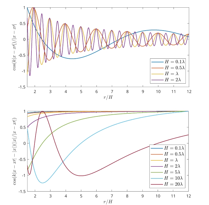
Figure 3: Source point factorization test. Consider an origin centered box of side $H$. In this illustration, the source point is positioned at ${\boldsymbol{x}}^{\prime}=(0,0,H/2)$, and the point ${\boldsymbol{x}}$ varies on the line $t(1,0,0)$ for $t\in[3H/2,12H]$. The graph at the top displays the real part of the kernel $G({\boldsymbol{x}},{\boldsymbol{x^{\prime}}})$, which illustrates a highly-oscillatory behavior even for the smaller size boxes. The bottom graph illustrates the slow oscillatory behavior of the analytic factor $g_{S}({\boldsymbol{x}},{\boldsymbol{x^{\prime}}})$ for boxes as large as $H=20\lambda$.

As discussed in the next section, the IFGF method approximates the contribution $I_{S}({\boldsymbol{x}}_{\ell}^{T})$ only at target points which are at least one box away. For such target points, we have $(s,\theta,\phi)\in\mathcal{E}=[0,\eta]\times[0,\pi]\times[0,2\pi)$, where $\eta=\sqrt{3}/3<1$. Hence, using the analytic and low-oscillatory characteristics of $g_{S}$, and by linearity, the analytic factor contribution $F_{S}({\boldsymbol{x}}_{\ell}^{T})$ can efficiently be interpolated in the $(s,\phi,\theta)$ variables with a few finite interpolation intervals in the $s$ variable, in conjunction with a number of adequately selected compact interpolation intervals in the $\phi$ and $\theta$ variables. Once $F_{S}({\boldsymbol{x}}_{\ell}^{T})$ has been interpolated, the value of $I_{S}({\boldsymbol{x}}_{\ell}^{T})$ can be obtained by multiplying the centered factor $G({\boldsymbol{x}}_{\ell}^{T},{\boldsymbol{x}}^{S})$, which is known analytically.

To appropriately structure the interpolation, the domain ${\mathcal{E}}$ is partitioned as described in what follows. For given positive integers $n_{s}$ and $n_{a}$, we denote the length of the interpolation intervals in $s$, and in the angular variables $\theta$ and $\phi$ as

$$\Delta_{s}=\frac{\eta}{n_{s}}\;\mathrm{and}\;\Delta_{\theta}=\Delta_{\phi}=\frac{\pi}{n_{a}},$$ (43)

respectively. Then for each $\gamma=(\gamma_{1},\gamma_{2},\gamma_{3})$ in $K_{C}:=\{1,\dots,n_{s}\}\times\{1,\dots,n_{a}\}\times\{1,\dots,2n_{a}\},$ the interpolation intervals $E^{s}_{\gamma_{1}}$, $E^{\theta}_{\gamma_{2},\gamma_{3}}$ and $E^{\phi}_{\gamma_{3}}$ along the $s$, $\theta$, and $\phi$ directions are defined by

$$E^{s}_{\gamma_{1}}=[(s-1)\Delta_{s},s\Delta_{s})$$ (44)

$$E^{\theta}_{\gamma_{2},\gamma_{3}}=\begin{cases}[(n_{a}-1)\Delta_{\theta},\pi]&\mathrm{for}\;\gamma_{2}=n_{a},\gamma_{3}=2n_{a}\\ (0,\Delta_{\theta})&\mathrm{for}\;\gamma_{2}=1,\gamma_{3}>1\\ [(\gamma_{2}-1)\Delta_{\theta},\gamma_{2}\Delta_{\theta}]&\mathrm{otherwise},\end{cases}$$ (45)

$$E^{\phi}_{\gamma_{3}}=[(\gamma_{3}-1)\Delta_{\phi},\gamma_{3}\Delta_{\phi}).$$ (46)

For each $\gamma=(\gamma_{1},\gamma_{2},\gamma_{3})\in K_{C}$, we call

$$E_{\boldsymbol{\gamma}}:=E^{s}_{\gamma_{1}}\times E^{\theta}_{\gamma_{2}}\times E^{\phi}_{\gamma_{3}}$$ (47)

a cone domain, and the image of $E_{\boldsymbol{\gamma}}$ under the parametrization (40)

$$C_{\boldsymbol{\gamma}}({\boldsymbol{x}}^{S}):=\{{\boldsymbol{x}}=x(s,\theta,\phi;{\boldsymbol{x}}^{S}):((s,\theta,\phi)\in E_{\boldsymbol{\gamma}})\},$$ (48)

a cone segment (see Fig. 4 for an analogous two-dimensional illustration for cone-structure for a single box.)

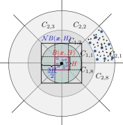
Figure 4: Illustration of a cone structure for a single box in 2D. The figure illustrates a cone-structure for the box $B({\boldsymbol{x}},H)$ shown in red, the neighborhood boxes in $\mathcal{N}B({\boldsymbol{x}},H)$ separated by dashed lines within thick black lines, and a $P_{s}\times P_{a}=3\times 3$ interpolation scheme in cone-segment $C_{2,1}$. The hollow blue star-shape points denote the source points within $B({\boldsymbol{x}},H)$, blue solid circles denote the interpolation grid points in $C_{2,1}$, and the points denotes by black-$+$ signs are the target points within $C_{2,1}$. The IFGF method does not interpolate contribution from $B({\boldsymbol{x}},H)$ at any target point that lies within $\mathcal{N}B({\boldsymbol{x}},H)$.

We point out that by definition, ${\mathcal{E}}=\cup_{\boldsymbol{\gamma}\in K_{C}}C_{\boldsymbol{\gamma}}({\boldsymbol{x}}^{S})$ and $C_{\boldsymbol{\gamma}}({\boldsymbol{x}}^{S})\cap C_{\boldsymbol{\gamma}^{\prime}}({\boldsymbol{x}}^{S})=\emptyset$ for $\boldsymbol{\gamma}\neq\boldsymbol{\gamma}^{\prime}$.

In each cone segment $C_{\boldsymbol{\gamma}}$, the IFGF algorithm uses 1D Chebyshev interpolation strategy in each of the radial and angular variables with a fixed numbers $P_{s}$ and $P_{a}$ of interpolation points along the radial and the angular variables, respectively. For a function $f:[-1,1]\rightarrow\mathbb{C},$ the 1D Chebyshev interpolating polynomial of degree $(n-1)$ is given by

$$I^{n}f(x)=\sum_{i=0}^{n-1}\widetilde{w}_{i}T_{i}(x),\quad x\in[-1,1],$$ (49)

where $T_{i}$ is the Chebyshev polynomial of degree $i$ and the weights $\widetilde{w}_{i}$ are given by

$$\widetilde{w}_{i}=\frac{2}{n}{\sum}_{j=0}^{n-1}c_{j}f(x_{j})T_{i}(x_{j}),\quad\mathrm{for}\;i=0,\dots,n-1$$ (50)

with $c_{0}=0.5$ and $c_{i}=1$ for $i=1,\dots,n-1$, and the points $x_{j}$ are given by (16) for $n=N_{C}$.

III-G IFGF Multilevel Recursive Interpolation.

To achieve the desired acceleration with a $\mathcal{O}(N\log N)$ computational cost, the proposed method utilizes the multi-level IFGF recursive-interpolation strategy introduced in [1] for the Helmholtz problem. The multi-level IFGF method implements the interpolation strategy described for a single box in Section III-F in a recursive manner using larger and larger boxes, where the contributions of the larger boxes are in turn evaluated by interpolation and accumulation of the contributions from the smaller boxes.

The multi-level IFGF method starts by selecting a single cubic box $B({\boldsymbol{x}}_{(1,1,1)},H_{1})\supset\Gamma_{N}$ (see Fig. 5) containing all the source points. Then, starting from this topmost level-$d=1$ box $B({\boldsymbol{x}}_{(1,1,1)},H_{1})$, the IFGF method creates the level-$d$ boxes for $d=2,\dots,D$, by partitioning each level-$(d-1)$ boxes into eight disjoint, equisized “children” boxes $B^{d}_{\boldsymbol{\mathrm{k}}}=B({\boldsymbol{x}}_{\boldsymbol{k}},H_{d})$ of side $H_{d}=H_{d-1}/2$, and centered at

$${\boldsymbol{x}}^{d}_{\boldsymbol{\mathrm{k}}}:={\boldsymbol{x}}^{1}_{\boldsymbol{1}}-\frac{H_{1}}{2}\boldsymbol{1}+\frac{H_{d}}{2}(2\boldsymbol{\mathrm{k}}-\boldsymbol{1}),\;(\boldsymbol{\mathrm{k}}\in\mathrm{K}^{d}_{B}=\{1,\dots,2^{d-1}\}^{3}).$$

Each box $B^{d}_{\boldsymbol{\mathrm{k}}}$ for $d=2,\dots,D$ is contained in a “parent box” on level-($d-1$), which is denoted by $\mathcal{P}B^{d}_{\boldsymbol{\mathrm{k}}}$. The value of $D$ is chosen so that the side $H_{D}$, corresponding to the side length of a box on the lowest level, satisfies the condition $H_{D}\leq 0.25\lambda$, where $\lambda$ is the wavelength. It is only necessary to keep track of the “relevant boxes”, that is, the boxes $B^{d}_{\boldsymbol{\mathrm{k}}}$ for which $B^{d}_{\boldsymbol{\mathrm{k}}}\cap\Gamma_{N}\neq\emptyset$. The set of all relevant boxes of level $d$ ($d=1,\dots,D$) is denoted by

$$\mathcal{R}^{d}_{B}:=\{B^{d}_{\boldsymbol{\mathrm{k}}}:B^{d}_{\boldsymbol{\mathrm{k}}}\cap\Gamma_{N}\neq\emptyset;\boldsymbol{\mathrm{k}}\in\mathrm{K}^{d}_{B}\}.$$ (51)

The totality of the above box hierarchy is stored as a linear octree.

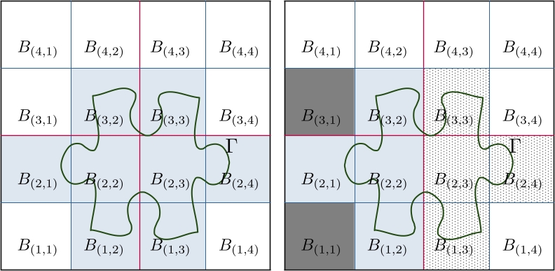
Figure 5: Illustration for box-hierarchy in 2D for $D=3$. The level $1$ box (the largest box) is always relevant as it contains the set $\Gamma_{N}$. Here, the all four level-$2$ boxes (divided by the red lines) are relevant as well. On level $3$–On left: only the light shaded boxes on the left image above are relevant as the other boxes do not intersect with the surface $\Gamma$. On right: for the box $B_{(2,1)}$, only the light shaded boxes are in $\mathcal{N}B_{(2,1)}$ whereas the dot-pattern boxes are in the cousin box set $\mathcal{M}B_{(2,1)}$. Note that the dark shaded boxes $B_{(1,1)}$ and $B_{(3,1)}$ not being relevant are not considered neighbors of $B_{(2,1)}$ (54).

Utilizing (38) and (39), the field generated by the sources within a relevant box $B^{d}_{\boldsymbol{\mathrm{k}}}$ are given by

$$I^{d}_{\boldsymbol{\mathrm{k}}}({\boldsymbol{x}})=G({\boldsymbol{x}},{\boldsymbol{x}}^{d}_{\boldsymbol{\mathrm{k}}})F^{d}_{\boldsymbol{\mathrm{k}}}({\boldsymbol{x}});\;F^{d}_{\boldsymbol{\mathrm{k}}}({\boldsymbol{x}})=\!\!\!\!\displaystyle\sum_{{\boldsymbol{x^{\prime}}}\in B^{d}_{\boldsymbol{\mathrm{k}}}\cap\Gamma_{N}}\!\!\!\!\!\!\!a({\boldsymbol{x^{\prime}}})g^{d}_{\boldsymbol{\mathrm{k}}}({\boldsymbol{x}},{\boldsymbol{x^{\prime}}}).$$ (52)

Moreover, using (40)

$$F^{d}_{\boldsymbol{\mathrm{k}}}({\boldsymbol{x}})=F^{d}_{\boldsymbol{\mathrm{k}}}(s,\theta,\phi)=\displaystyle\sum_{{\boldsymbol{x^{\prime}}}\in B^{d}_{\boldsymbol{\mathrm{k}}}\cap\Gamma_{N}}\!\!\!\!\!\!\!a({\boldsymbol{x^{\prime}}})g^{d}_{\boldsymbol{\mathrm{k}}}(s,\theta,\phi,{\boldsymbol{x^{\prime}}})$$ (53)

where the spherical coordinate $(s,\theta,\phi)$ is centered at ${\boldsymbol{x}}^{d}_{\boldsymbol{\mathrm{k}}}$. As discussed in what follows, the multilevel recursive interpolation strategy relies on the application of the single box interpolation strategy to evaluate the analytic factor $F^{d}_{\boldsymbol{\mathrm{k}}}(s,\theta,\phi)$ for each one of the relevant boxes starting at level-$D$, and then iteratively proceeding to level-$3$; at this level for a given target point ${\boldsymbol{x}}\in B^{d}_{\boldsymbol{\mathrm{k}}}$ contributions from all the non-neighbor boxes are accumulated. The contribution from the sources within the “neighbor boxes” (defined in what follows) are computed using the CBIE method as discussed earlier in Sections III-C and III-D.

To facilitate the recursive interpolation strategy, several additional concepts are required. Following [1], we define for a given level-$d$ box $B^{d}_{\boldsymbol{\mathrm{k}}}$, the set $\mathcal{N}B^{d}_{\boldsymbol{\mathrm{k}}}$ of all level-$d$ boxes that are neighbors of $B^{d}_{\boldsymbol{\mathrm{k}}}$ (that is a box that shares a side with the box $B^{d}_{\boldsymbol{\mathrm{k}}}$) and, the set $\mathcal{M}B^{d}_{\boldsymbol{\mathrm{k}}}$ of all level-$d$ boxes that are cousins of $B^{d}_{\boldsymbol{\mathrm{k}}}$ (the non-neighboring boxes which are children of a neighbor of the parent box $\mathcal{P}B^{d}_{\boldsymbol{\mathrm{k}}}$). Similarly, the set $\mathcal{U}B^{d}_{\boldsymbol{\mathrm{k}}}$ of neighbor points and the set $\mathcal{V}B^{d}_{\boldsymbol{\mathrm{k}}}$ of cousin points of $B^{d}_{\boldsymbol{\mathrm{k}}}$ are defined as the set of all points in $\Gamma_{N}$ that are contained in the neighbor and the cousin boxes of $B^{d}_{\boldsymbol{\mathrm{k}}}$, respectively. We thus have

$$\mathcal{N}B^{d}_{\boldsymbol{\mathrm{k}}} :=\{B^{d}_{\boldsymbol{\mathrm{j}}}\in\mathcal{R}^{d}_{B}:\lVert\boldsymbol{\mathrm{j}}-\boldsymbol{\mathrm{k}}\rVert\leq 1\}$$ (54)

$$\mathcal{M}B^{d}_{\boldsymbol{\mathrm{k}}} :=\{B^{d}_{\boldsymbol{\mathrm{j}}}\in\mathcal{R}_{B}:B^{d}_{\boldsymbol{\mathrm{j}}}\notin\mathcal{N}B^{d}_{\boldsymbol{\mathrm{k}}}\wedge\mathcal{P}B^{d}_{\boldsymbol{\mathrm{j}}}\in\mathcal{NP}B^{d}_{\boldsymbol{\mathrm{k}}}\}$$ (55)

$$\mathcal{U}B^{d}_{\boldsymbol{\mathrm{k}}} :=\left(\bigcup_{B\in\mathcal{N}B^{d}_{\boldsymbol{\mathrm{k}}}}B\right)\cap\Gamma_{N}$$ (56)

$$\mathcal{V}B^{d}_{\boldsymbol{\mathrm{k}}} :=\left(\bigcup_{B\in\mathcal{M}B^{d}_{\boldsymbol{\mathrm{k}}}}B\right)\cap\Gamma_{N}$$ (57)

Figure 5 (see captions thereof) illustrates an analogous two-dimensional box-hierarchy for $D=3$ and the aforementioned concepts, namely, relevant boxes, neighbors and cousins.

As alluded to in the single box interpolation discussion in Section III-F, the interpolation of the analytic factor $F^{d}_{\boldsymbol{\mathrm{k}}}(s,\theta,\phi)$ associated with a level-$d$ relevant box $B^{d}_{\boldsymbol{\mathrm{k}}}$ relies on level-$d$ cone segments, which are denoted by

$$C^{d}_{\boldsymbol{\mathrm{k}};\boldsymbol{\gamma}}=C_{\boldsymbol{\gamma}}({\boldsymbol{x}}^{d}_{\boldsymbol{\mathrm{k}}}),\;\boldsymbol{\gamma}\in K^{d}_{C}$$ (58)

where $K^{d}_{C}:=\{1,\dots,n_{s;d}\}\times\{1,\dots,n_{a;d}\}\times\{1,\dots,2n_{a;d}\}$ for certain selection of integers $n_{s}=n_{s;d}$ and $n_{a}=n_{a;d}$ appropriately chosen to ensure the desired accuracy (see Remark 2). Analogous to the relevant boxes, the IFGF method also uses the concept of “relevant cone segments”. Denoting the set of interpolation points within the cone segments $C^{d}_{\boldsymbol{\mathrm{k}};\boldsymbol{\gamma}}$ by $\mathcal{X}C^{d}_{\boldsymbol{\mathrm{k}};\boldsymbol{\gamma}}$; the set $\mathcal{R}_{C}B^{d}_{\boldsymbol{\mathrm{k}}}$ of the cone segments relevant to the box $B^{d}_{\boldsymbol{\mathrm{k}}}$ are defined recursively starting from level $d=3$ as follows:

$$\mathcal{R}_{C}B^{d}_{\boldsymbol{\mathrm{k}}} :=\emptyset\;\mathrm{for}\;d=1,2,\,\mathrm{and,}$$

$$\mathcal{R}_{C}B^{d}_{\boldsymbol{\mathrm{k}}} :=\Big{\{}C^{d}_{\boldsymbol{\mathrm{k}};\boldsymbol{\gamma}}:C^{d}_{\boldsymbol{\mathrm{k}};\boldsymbol{\gamma}}\cap\mathcal{V}B^{d}_{\boldsymbol{\mathrm{k}}}\neq\emptyset\,\mathrm{or}\,C^{d}_{\boldsymbol{\mathrm{k}};\boldsymbol{\gamma}}\cap\Big{(}\bigcup_{C\in\mathcal{R}\mathcal{P}B^{d}_{\boldsymbol{\mathrm{k}}}}\mathcal{X}C\Big{)}\neq\emptyset\Big{\}}$$

for $\boldsymbol{\mathrm{k}}\in\mathrm{K}^{d}_{B}$ and $d\geq 3$. Thus, a level-$d$ cone segment $C^{d}_{\boldsymbol{\mathrm{k}};\boldsymbol{\gamma}}$ is recursively (starting from $d=3$ to $d=D$) defined to be relevant to a box $B^{d}_{\boldsymbol{\mathrm{k}}}$ if either, (1) it includes a surface discretization point in a cousin of $B^{d}_{\boldsymbol{\mathrm{k}}}$, or if, (2) it includes an interpolation point of a relevant cone segment associated with the parent box $\mathcal{P}B^{d}_{\boldsymbol{\mathrm{k}}}$ of $B^{d}_{\boldsymbol{\mathrm{k}}}$. The set of all relevant level-$d$ cone-segments is given by

$$\mathcal{R}_{C}^{d}\coloneqq\{C^{d}_{\boldsymbol{\mathrm{k}};\boldsymbol{\gamma}}\in\mathcal{R}_{C}B^{d}_{\boldsymbol{\mathrm{k}}}:\boldsymbol{\gamma}\in K^{d}_{C},\boldsymbol{\mathrm{k}}\in K^{d}_{B}~{}\mathrm{and}~{}B^{d}_{\boldsymbol{\mathrm{k}}}\in\mathcal{R}^{d}_{B}\}.$$ (59)

Remark 2 (Choosing cone-structure sizes.)

In view of Theorems 1 and 2 in [1], which in particular imply that the use of fixed numbers $n_{s}$ and $n_{a}$ give rise to essentially constant cone-segment interpolation errors for all $H$-side boxes satisfying $\kappa H<1$, and the pertaining discussion in [1, Section 3.3.1], the IFGF algorithm chooses the values of $n_{s;d}$ and $n_{a;d}$ as described in what follows. Starting from certain selection of $n_{s;(D+1)}$ and $n_{a;(D+1)}$ as the initial values, the method selects the value of $n_{s;d}$ and $n_{a;d}$ for $d=D,D-1,\dots,3,$ according to the rule $n_{s;d}=a_{d}n_{s;(d-1)}$ and $n_{a;d}=a_{d}n_{a;(d-1)}$ where $a_{d}=1$ if $\kappa H_{d}\leq 1/2$, and $a_{d}=2$ in the complementary case. In keeping with [1], in each cone-segment we have used the values $P_{s}=3$ and $P_{a}=5$ for all the numerical experiments presented in this work.

As mentioned above, the IFGF method evaluates the discrete integrator by commingling the effect of large numbers of sources into a small number of interpolation parameters; which is possible, in particular, owing to the analytic property and slow-oscillatory character of the analytic factor $g^{d}_{\boldsymbol{\mathrm{k}}}$. We note that at the level $D$, the contribution of the sources within a box $B^{D}_{\boldsymbol{\mathrm{k}}}$ at the relevant cone-segment interpolation points are produced by directly evaluating the sum $F^{D}_{\boldsymbol{\mathrm{k}}}$. A summary of the algorithm is presented below.

1. Determine the sets of relevant boxes $\mathcal{R}_{B}$ (51) and of relevant cone-segments $\mathcal{R}^{d}_{C}$ (59) for all $d=1,\dots,D$.

2. Direct evaluations on level $D$.
   –For every D-level box evaluate the field $I^{D}_{\boldsymbol{\mathrm{k}}}$ at all the neighboring target points ${\boldsymbol{x}}\in\mathcal{U}B^{D}_{\boldsymbol{\mathrm{k}}}$ using the CBIE method.
   –For every D-level relevant box $B^{D}_{\boldsymbol{\mathrm{k}}}\in\mathcal{R}_{B}$ evaluate the analytic factor $F^{D}_{\boldsymbol{\mathrm{k}}}$ at all the interpolation points ${\boldsymbol{x}}\in\mathcal{X}C^{D}_{\boldsymbol{\boldsymbol{\mathrm{k}}};\boldsymbol{\gamma}}$ of the relevant cone segments $C^{D}_{\boldsymbol{\boldsymbol{\mathrm{k}}};\boldsymbol{\gamma}}\in\mathcal{R}_{C}B^{D}_{\boldsymbol{\mathrm{k}}}$ by direct evaluation of the sum (53).

3. Interpolation for $d=D,\dots,3$.
   –For every relevant box $B^{d}_{\boldsymbol{\mathrm{k}}}$ evaluate the field $I^{d}_{\boldsymbol{\mathrm{k}}}({\boldsymbol{x}})$ at every surface discretization point ${\boldsymbol{x}}\in\mathcal{V}B^{d}_{\boldsymbol{\mathrm{k}}}$ by interpolation of the analytic factor $F^{d}_{\boldsymbol{\mathrm{k}}}$ and multiplication by the centered factor $G({\boldsymbol{x}},{\boldsymbol{x}}^{d}_{\boldsymbol{\mathrm{k}}})$.
   –For every level-$d$ relevant box $B^{d}_{\boldsymbol{\mathrm{k}}}$ determine the parent box $B^{d-1}_{\boldsymbol{\mathrm{j}}}=\mathcal{P}B^{d}_{\boldsymbol{\mathrm{k}}}$ and, obtain the analytic factor $F^{d-1}_{\boldsymbol{\mathrm{j}}}$ at all level-$(d-1)$ interpolation points corresponding to $B^{d-1}_{\boldsymbol{\mathrm{j}}}$ by first, interpolation of $F^{d}_{\boldsymbol{\mathrm{k}}}$ and then re-centering by multiplying the smooth factor $G({\boldsymbol{x}},{\boldsymbol{x}}^{d}_{\boldsymbol{\mathrm{k}}})/G({\boldsymbol{x}},{\boldsymbol{x}}^{d-1}_{\boldsymbol{\mathrm{j}}})$, and finally, accumulating the contributions from all the children boxes of $B^{d-1}_{\boldsymbol{\mathrm{j}}}$.

For a more detailed description of the IFGF acceleration strategy, including an analysis of its computational complexity, we refer to [1].

III-H Local Corrections to IFGF Sum.

For evaluation of $I^{D}_{\boldsymbol{\mathrm{k}}}$ at the points ${\boldsymbol{x}}_{\ell}\in\mathcal{U}B^{D}_{\boldsymbol{\mathrm{k}}}$ the method relies on the CBIE part of the method. As discussed in Section III-A, the method uses a non-overlapping patch decomposition of the surface $\Gamma$, and certain changes of variables on a refined grid to resolve the singular behavior of the kernel when the source and the target points are in close proximity. It becomes necessary to compute the total contribution from all the source points within a patch as the quadrature is target point specific. Clearly, the surface decomposition does not conform to the 3D boxes, and some of the patches covering the neighbor set $\mathcal{N}B^{D}_{\boldsymbol{\mathrm{k}}}$ may intersect the cousin set $\mathcal{M}B^{D}_{\boldsymbol{\mathrm{k}}}$. Note that if any of these intersecting patches, say, $\Gamma_{p}$ is singular for a point ${\boldsymbol{x}}\in B^{D}_{\boldsymbol{\mathrm{k}}}$, that is, $p\in\mathscr{S}_{\ell}$ (see (20)) then some contribution from these patches, for example, the region $\Gamma_{p_{6}}\setminus\mathcal{N}B^{D}_{\boldsymbol{\mathrm{k}}}$ as per the illustration in Figure 6, is counted both by the CBIE and the IFGF part of the algorithm, which requires a correction. We note that these corrections can be applied at the beginning of a run by subtracting the product of Fejér quadrature weight and the kernel value from the precomputed singular weights for all such instances.

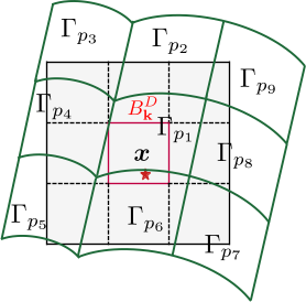
Figure 6: Illustration for local correction in 2D.

III-I IFGF for EM Problem.

In Section III-G, we have discussed the recursive IFGF interpolation strategy for a single density $\phi$. For the EM problem, as mentioned at the beginning of Section III, we must carry out the interpolation strategy for eight scalar quantities, and we also need to compute the normal derivative of the single layer (SL) potentials as well.
Computing Normal Derivative. To compute the normal derivative of the SL potentials, we use finite differences, in particular, we use the (first order) forward difference formula

$$D[\phi]({\boldsymbol{x}})=\frac{S[\phi](\widetilde{{\boldsymbol{x}}}_{{\boldsymbol{n}}})-S[\phi]({\boldsymbol{x}})}{|{\boldsymbol{n}}\cdot\boldsymbol{h}|}$$ (60)

where $\widetilde{{\boldsymbol{x}}}_{{\boldsymbol{n}}}={\boldsymbol{x}}+{\boldsymbol{n}}\cdot\boldsymbol{h}$ and $\boldsymbol{h}=(h,h,h)^{t}$ with one-dimensional step-size $h=|{\boldsymbol{n}}\cdot\boldsymbol{h}|=10^{-6}$. Hence, to compute the normal derivative we need to evaluate the interpolation at one extra point for each density for which the normal derivative is required. To obtain the value $S[\phi](\widetilde{{\boldsymbol{x}}_{n}})$ for a surface discretization point ${\boldsymbol{x}}\in B^{d}_{\boldsymbol{\mathrm{k}}}$, the method uses the same interpolation procedure. In particular, to obtain the contribution to the normal derivative $D[\phi]({\boldsymbol{x}})$ from a cousin box $B\in\mathcal{M}B^{d}_{\boldsymbol{\mathrm{k}}}$, the method uses the relevant cone-segment containing the point ${\boldsymbol{x}}$ to interpolate at the point $\widetilde{{\boldsymbol{x}}}_{{\boldsymbol{n}}}$ in addition to the point ${\boldsymbol{x}}$ itself. Then the formula (60) is used to approximate the contribution to the normal derivative at ${\boldsymbol{x}}$ coming from a cousin box. Note that for a given point ${\boldsymbol{x}}\in\Gamma_{N}$, it is possible for the point $\widetilde{{\boldsymbol{x}}}_{{\boldsymbol{n}}}$ to lie in a different cone-segment, which leads to extrapolation instead of interpolation. The point $\widetilde{{\boldsymbol{x}}}_{{\boldsymbol{n}}}$ may also lie within the neighbor boxes. Both situations, due to the small finite-difference step-size $h$, do not affect the accuracy as demonstrated by the numerical experiments presented in Section IV.

IFGF for Multiple Densities: Speed-vs-Memory Trade-off.
As mentioned in the beginning of this section, in order to efficiently approximate the integral operators associated with (7), we need to use the IFGF interpolation strategy for eight densities and two kernel values arising from two different domains. The straightforward approach would be to use the IFGF algorithm once for each combination of a density and a kernel, which here onward we call $\mathrm{IFGF}_{Seq}$. In this approach, we are required to traverse the box-octree a total number of sixteen times. A different approach would be to interpolate the integrals for all the densities and the kernels at one go, which we refer to as $\mathrm{IFGF}_{Vec}$. In the later approach, we need to traverse the box-octree only once. More importantly, in the second, the kernel values for a given pair of source and target points only need to be computed once for all the densities, leading to a further speedup of the overall IFGF strategy in the context of the EM problem compared to the $\mathrm{IFGF}_{Seq}$ approach (see Fig. 7). We point out that in the $\mathrm{IFGF}_{Seq}$ approach, we need to store the interpolation weights only for one combination of a density and a kernel at any time whereas in the $\mathrm{IFGF}_{Vec}$ approach, we need to store the interpolation weights for all sixteen possible combinations of the densities and both the kernels simultaneously, which requires sixteen times the memory for storing the interpolation weights in comparison to the first approach.

For this work, we chose the second option, which leverages uses the same IFGF algorithm, but for an array of densities and an array of kernels, to save on the run time (see Remark 3). In particular, the input weights to the IFGF algorithm for the EM problem can be written as $W=(a_{k,\ell})_{8\times N}$. Denoting by $I_{k,n}$ the sum for $k$-th density and $n$-th kernel, and denoting the two kernels by $G_{1}$ and $G_{2}$, the EM version of equation (34) can be written as

$$\begin{split}\begin{bmatrix}I_{1,1}(x_{\ell})&I_{1,2}(x_{\ell})\\ \vdots&\vdots\\ I_{8,1}(x_{\ell})&I_{8,2}(x_{\ell})\end{bmatrix}&\\ :=\sum_{\begin{subarray}{c}m=1\\ m\neq\ell\end{subarray}}^{N}\begin{bmatrix}a_{1,m}\\ \vdots\\ a_{8,m}\end{bmatrix}&\begin{bmatrix}G_{1}({\boldsymbol{x}}_{\ell},{\boldsymbol{x}}_{m})&G_{2}({\boldsymbol{x}}_{\ell},{\boldsymbol{x}}_{m})\end{bmatrix},\end{split}$$ (61)

for $\ell=1,\dots,N$. The evaluation of (61) then follows the steps of the IFGF algorithm prescribed in Section III-G. This concludes the discussion on the numerical scheme of the proposed methodology.

Remark 3 (On selection of IFGF approach)

One can choose to approximate the discrete sum for a specific number of densities or kernels at a time. For instance, we can evaluate the sum for all eight densities, but for a single kernel at a time; this reduces the memory requirement of the interpolation weights exactly by half, and (in our experiments) shows $\approx 1.5\times$ slower run time compared to $\mathrm{IFGF}_{Vec}$. Moreover, the memory required by the interpolation weights can easily be computed once we know the number of relevant cone segments; and one can choose an approach at run time based on the available memory.

IV Numerical Experiments

In this section, we present results from several numerical experiments. In all the examples presented, equal numbers of mesh points are used in $u$ and $v$ variables to discretize each patch. For the IFGF interpolation, $P_{s}=3$, and $P_{a}=5$ values were used in the radial and angular directions, respectively. In addition, we have used the values $n_{s;D+1}=1$ and $n_{a;D+1}=2$ (see (58)) to structure the cone-hierarchy. For the incident field, we considered the planewave ${\boldsymbol{E}}^{\mathrm{inc}}=\exp(-i\kappa_{e}z)\hat{\boldsymbol{x}}$ in all cases, except in Example IV-E, where an electric dipole was used instead. We recall that $N=PN^{2}_{C}$ denotes the discretization size (III-A) (the total number of unknowns is $4N$), $P$ denotes the number of decomposing patches (13), and $N_{C}$ denotes the number of points per patch in one variable (16). We start the experiments with a forward map computation for a spherical geometry to study the time and accuracy of the CBIE-IFGF method. In addition, for the spherical geometry, we study the scattering simulation, as in this case the Mie series solution is available to compute the accuracy of the proposed method. Next, in order to demonstrate the applicability and the performance of the CBIE-IFGF method for arbitrarily shaped geometries, we also consider several different CAD models, namely, a glider model in Example IV-C, a hummingbird model in Example IV-D, and a Gmsh-rendered nanophotonic power splitter in Example IV-E. Run times of one forward map computation of the accelerated CBIE-IFGF method are provided for all examples and compared against that of the unaccelerated CBIE method. Note that the unaccelerated CBIE method implementation includes certain additional optimizations (e.g., reduced number of kernel evaluations due to shared kernels between densities) that are unavailable for the CBIE-IFGF method. The simulations for all the numerical results presented in this work were run on $128$ cores of an Ubuntu server equipped with two AMD EPYC $7763$ $64$-Core Processors (CPU speed: max $3.5$ GHz and min $1.5$ GHz) and a total of $1$TB available RAM. The GMRES residual tolerance was set to $10^{-4}$.

IV-A Forward Map Computation

As a first experiment, we study the timings and the accuracy of the proposed (accelerated) CBIE-IFGF forward map (FM)—namely, the action of the discretized version of the operators in the l.h.s. of (7) on a given set of densities. For this experiment, we consider $\Omega_{i}$ to be the unit sphere centered at the origin; $\Omega_{e}$ being the exterior $\mathbb{R}^{3}\setminus\Omega_{i}$ with $\epsilon_{e}=1,\epsilon_{i}=2.25$, and $\mu_{e}=\mu_{i}=1$. The refractive index of the interior medium is $1.5$. For this simulation, we have used the value $N_{C}=16$ (the smallest discretization in Table I has $P=24$ patches, and $P$ increases by a factor of four in each subsequent finer discretizations; this choice provides an accuracy of order $10^{-5}$ or better in the solution obtained using the CBIE method) to get an estimate of the accuracy provided by the CBIE-IFGF method. The Err. (FM) column in Table I shows the $\ell_{2}$-difference between the FM values obtained by the CBIE and the CBIE-IFGF methods. It shows that the FM operator values obtained using the CBIE-IFGF method match with that of the CBIE method with a fixed $10^{-4}$ accuracy, while maintaining a fixed number of points per wavelength. (Note that the choice of the $N_{C}$-value does not affect the accuracy provided by the IFGF interpolation strategy.)

The $T_{C}$ and the $T_{CI}$ columns in Table I represent the runtime of the FM of the CBIE and the CBIE-IFGF methods, respectively; whereas the column $T_{IFGF}$ shows the required runtime of only the $\mathrm{IFGF}_{Vec}$ interpolation part of the algorithm. Additionally, for comparison, the column $T_{Seq}$ lists the runtime of only the $\mathrm{IFGF}_{Seq}$ interpolation strategy. The run times, as illustrated in Fig. 7, are consistent with the $\mathcal{O}(N\log N)$ nature of the algorithm. We note that there is an increase in the runtime by a factor $\approx 4$ in the $\mathrm{IFGF}_{Seq}$ approach in comparison to the $\mathrm{IFGF}_{Vec}$ strategy.

IV-B Scattering from Spherical Geometry.

For the second numerical experiment, we consider scattering by the unit sphere. The materialistic properties and the parameter choices being same as in the previous example in IV-A except the value of $N_{C}$. Here we consider the value $N_{C}=12$ (which, as demonstrated in Table II, is sufficient to achieve an accuracy of the order of $10^{-4}$). The Err.(CBIE) and Err.(C-I) columns in Table II present the $\ell_{2}$-error in the computed field values produced by the unaccelerated CBIE method and the accelerated CBIE-IFGF method, respectively. The error is computed against the Mie series solution at $1000$ points on the surface of the origin centered sphere with a radius of $0.7$. In all the cases, a $10^{-4}$ accuracy is maintained by the CBIE-IFGF method.

$N$	$\kappa_{i}$	$T_{C}$	$T_{CI}$	$T_{IFGF}$	Err. (FM)	$T_{Seq}$
$6144$	$3\pi$	$0.064$	$0.12$	$0.076$	$1.0\cdot 10^{-4}$	$0.361$
$24576$	$6\pi$	$0.909$	$0.591$	$0.440$	$1.2\cdot 10^{-4}$	$1.88$
$98304$	$12\pi$	$13.05$	$2.84$	$2.25$	$1.3\cdot 10^{-4}$	$10.03$
$393216$	$24\pi$	$151.05$	$13.15$	$10.85$	$1.3\cdot 10^{-4}$	$40.38$
$1572864$	$48\pi$	$2463.5$	$58.14$	$50.14$	$1.4\cdot 10^{-4}$	$234.92$

TABLE I: Accuracy and run time study for the rectangular-polar method and IFGF-acceleration. $N_{C}=16$ points per patch (in one direction). $T_{C}$–runtime of CBIE FM, $T_{CI}$–runtime of CBIE-IFGF FM, $T_{IFGF}$–runtime of $\mathrm{IFGF}_{Vec}$, and $T_{Seq}$–run time for $\mathrm{IFGF}_{Seq}$.

$N$	$\kappa_{i}$	Iter.(CBIE)	Err.(CBIE)	Iter.(C-I)	Err.(C-I)
$3456$	$3\pi$	$26$	$8.8\cdot 10^{-5}$	$27$	$9.71\cdot 10^{-5}$
$13824$	$6\pi$	$45$	$7.80\cdot 10^{-5}$	$48$	$9.09\cdot 10^{-5}$
$55296$	$12\pi$	$91$	$4.45\cdot 10^{-5}$	$102$	$1.16\cdot 10^{-4}$
$221184$	$24\pi$	$158$	$1.28\cdot 10^{-4}$	$167$	$1.66\cdot 10^{-4}$
$884736$	$48\pi$	$-$	$-$	$443$	$3.82\cdot 10^{-4}$

TABLE II: Accuracy in the GMRES solution for the unaccelerated CBIE method and the CBIE-IFGF method.

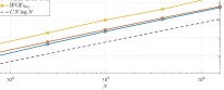
Figure 7: Various run times in $\log-\log$ scale of are presented. The legends “$\mathrm{IFGF}_{Seq}$” and “$\mathrm{IFGF}_{Vec}$” present the run time of the corresponding IFGF approaches. The “CBIE-IFGF FM” legend displays the required run time for one FM computation of the CBIE-IFGF method.

For graphical presentations, we consider the values $\kappa_{e}=32\pi$ and $\kappa_{i}=48\pi$. Fig. 8 shows the real-part of $E_{x}$ of the computed total field scattered by the unit sphere on the faces of the origin centered cube with sides of length $24\lambda$. Fig. 9 presents the absolute value of the $x$-component of the computed total field on the $[-5,5]\times[-5,5]$ square on the $yz$-plane.

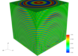
Figure 8: Real part of the field component $E_{x}$ for the computed total field scattered by the unit sphere on the faces of the origin centered cube with sides of length $24\lambda$. Field values are scaled to $[-1.5,1.5]$.

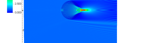
Figure 9: Absolute value of the $x$-component of the computed total field scattered by the unit sphere within the square $[-5,5]\times[-5,5]$ on the $yz$-plane. A (transparent) cross-section of the scattering sphere is inlaid in the figure. Field values are scaled to $[0,10]$.

IV-C Scattering From Glider CAD Model

For the second scattering example, we consider scattering simulation from the glider CAD model [27] with the following material properties: $\epsilon_{e}=\mu_{e}=1,\kappa_{e}=25.13$, and $\epsilon_{i}=2.16,\mu_{i}=1,\kappa_{i}=36.94$. The size of the scatterer is $45$ wavelengths in the longest dimension. The refractive index of the medium in $\Omega_{i}$ is $1.47$. The discretization contains $N\approx 320k$ points with $P=2225$ curvilinear patches and $N_{C}=12$ points per patch in each variable. The surface patch decomposition for this simulation is shown in Fig. 10. The accelerated CBIE-IFGF solver takes $\approx 9$ seconds on average for one FM calculation against $110$ seconds by the unaccelerated CBIE solver. Fig. 11 presents the real part and the absolute value of the $x$-component of the computed total field.

Figure 10: Patch configuration for the glider CAD model in the setting of Example IV-C.

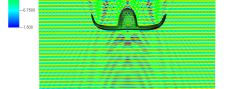
(a) Real part of $x$-component of the total field on the rectangle $[-7,7]\times[-7,7]$ on the $yz$-plane in the setting of Example IV-C.

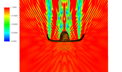
(b) Absolute value of $x$-component of the total field on the rectangle $[-7,7]\times[-7,7]$ on the $yz$-plane in the setting of Example IV-C.

Figure 11: Graphical presentation for the simulation in the setting of Example IV-C.

IV-D Scattering From Hummingbird NURBS CAD Model

Next, we consider the NURBS hummingbird model [28] with the following material properties: $\epsilon_{e}=\mu_{e}=1,\kappa_{e}=50.27$, and $\epsilon_{i}=2.16,\mu_{i}=1,\kappa_{i}=73.89$ with the wingspan of the scatterer being $77$ wavelengths. The refractive index of the medium in $\Omega_{i}$ is $1.47$. The discretization contains $N\approx 680k$ points with $P=4728$ curvilinear patches and $N_{C}=12$ points in each variable. The patch decomposition of the surface of the hummingbird model for this simulation is shown in Fig. 12. The accelerated solver takes $27$ seconds on average in one iteration against $588$ seconds (an average of five runs) by the unaccelerated solver. We plot the absolute value of the field component $E_{x}$ of the computed total field on the union of the truncated planes $x=-2$, $y=-1.5$, and $z=2$ in Fig. 13.

Figure 12: Patch configuration for the hummingbird model in the setup of numerical experiment described in Section IV-D.

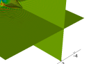
Figure 13: Absolute value of the field component $E_{x}$ on the cross-section of the $[-5,5]\times[-5,5]$ squares on the planes $x=-2$, $y=-1.5$, and $z=2$. Field values are scaled to $[0,1.5]$.

IV-E Scattering From Nanophotonic Splitter CAD Model

For the final numerical example, we consider a Gmsh-produced [16] geometry of a nanophotonic splitter [13] (with size $29\lambda_{i}$ in length) as depicted in Fig. 14. The material properties considered for this simulation are as follows: ($\epsilon_{e}=2.08$, $\mu_{e}=1$, $\kappa_{e}=5.85$) and ($\epsilon_{i}=12.08$, $\mu_{i}=1$, $\kappa_{i}=14.09$). The refractive indices within the domains $\Omega_{e}$ and $\Omega_{i}$ are $1.444$ and $3.476$, representing silicon dioxide and silicon respectively. An electric dipole was used to excite the input waveguide of the splitter. The surface is discretized with $P=280$ curvilinear patches with $N_{C}=12$ points per patch in each variable within each patch containing a total of $N\approx 40k$ points. For simulation in this experiment, in conjunction with the proposed method, we have additionally used a windowing function to properly truncate the integral operators, see [13] and the relevant references therein. The run time for one FM for the unaccelerated CBIE and the CBIE-IFGF methods are $2.49$ seconds and $0.52$ seconds, respectively, demonstrating that the CBIE-IFGF provides a 5x speed-up even for this relatively small-size problem. Fig. 15 and Fig. 16 show the real part and the absolute value, respectively, of the component $E_{y}$ of the computed total field on the rectangle $(x,y)\in[-1.5,6]\times[-2,2]$ on the $xy$-plane.

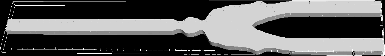
Figure 14: Shape of the nanophotonic splitter scatterer.

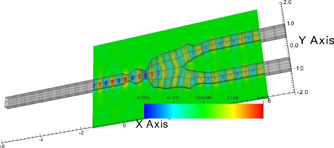
Figure 15: Real part of $E_{y}$.

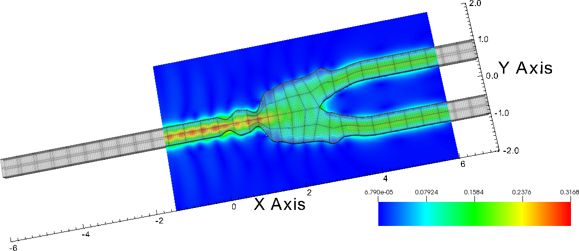
Figure 16: Absolute value of $E_{y}$.

V Summary

This paper presents an accelerated Nyström solver for the electromagnetic scattering problem for a dielectric medium. The method uses non-overlapping curvilinear parametric patches to decompose the surface, and approximates the density on a tensor-product of 1D Chebyshev grids in both the parametric variables. A polynomial change-of-variables-based strategy is used to resolve the singular behavior of the Green’s function in conjunction with the IFGF interpolation strategy to achieve an overall $\mathcal{O}(N\log N)$ computational complexity. We illustrated the accuracy and the efficiency of the proposed method with multiple numerical examples. Future work includes further acceleration of the EM scattering problem using GPU programming.

References

• [1] Christoph Bauinger and Oscar P. Bruno. “Interpolated Factored Green Function” method for accelerated solution of scattering problems in Journal of Computational Physics, volume 430, pages 110095, 2021.
• [2] Edwin Jimenez, Christoph Bauinger and Oscar P. Bruno. IFGF-accelerated high-order integral equation solver for acoustic wave scattering arXiv:2112.06316v3 [math.NA] 29 Oct 2022.
• [3] Oscar P. Bruno, Emmanuel Garza. A Chebyshev-based rectangular-polar integral solver for scattering by geometries described by non-overlapping patches in Journal of Computation Physics, volume 421, pages 109740, 2020.
• [4] David Colton, Rainer Kress. Inverse Acoustic and Electromagnetic Scattering Theory Second Edition, 1998, Springer-Verlag.
• [5] Jean-Claude Nédélec. Acoustic and Electromagnetics Equations: Integral Representations for Harmonic Problems First Edition, 2001, Springer-Verlag.
• [6] John L. Volakis, Kubilay Sertel. Integral Equation Methods for Electromagnetics Schitech Publishing Inc, Raleigh, NC.
• [7] Pasi Ylä-Oijala, Matti Taskinen. Well-conditioned Müller Formulation for Electromagnetic Scattering by Dielectric Objects in IEEE Transactions on Antennas and Propagation, Vol. 53, No. 10, October, 2005.
• [8] Roger F. Harrington. Boundary Integral Formulations for Homogeneous Material Bodies in Journal of Electromagnetic Waves and Applications 3, no. 1 (1989): 1–15.
• [9] A. Taflove and S. C. Hagness. Computational Electrodynamics: The Finite-Difference Time-Domain Method, 3rd ed. Norwood, MA, USA: Artech House, 2005.
• [10] C. M. Lalau-Keraly, S. Bhargava, O. D. Miller, and E. Yablonovitch. Adjoint shape optimization applied to electromagnetic design, Opt. Exp., vol. 21, no. 18, pp. 21693–21701, 2013.
• [11] Jin Hu, Emmanuel Garza, and Constantine Sideris. A Chebyshev-Based High-Order-Accurate Integral Equation Solver for Maxwell’s Equations IEEE Transactions on Antennas and Propagation, Vol. 69, No. 9, September 2021.
• [12] Constantine Sideris, Emmanuel Garza, and Oscar P. Bruno. Ultrafast Simulation and Optimization of Nanophotonic Devices with Integral Equation Methods ACS Photonics 6 (12), 3233-3240, 2019.
• [13] Emmanuel Garza and Constantine Sideris. Fast Inverse Design of 3D Nanophotonic Devices Using Boundary Integral Methods ACS Photonics 10 (4), 824-835, 2023.
• [14] Claus Müller. Foundations of the Mathematical Theory of Electromagnetic Waves Springer-Verlag, Berlin, Germany, 1969.
• [15] W. H. Press, S. A. Teukolsky, W. T. Vetterling, and B. P. Flannery. Numerical Recipes: The Art of Scientific Computing, 3rd ed. New York, USA, Cambridge University Press, 2007.
• [16] Christophe Geuzaine, Jean-François Remacle. Gmsh: A 3-D finite element mesh generator with built-in pre-and post-processing facilities. International Journal for Numerical Methods in Engineering 79, 1309–1331, 2009.
• [17] Emmanuel Garza. Boundary integral equation methods for simulation and design of photonic devices. Ph.D. thesis, California Institute of Technology, 2020.
• [18] Oscar Bruno, Tim Elling, Randy Paffenroth, Catalin Turc. Electromagnetic integral equations requiring small numbers of Krylov-subspace iterations, Journal of Computational Physics, Volume 228, Issue 17, Pages 6169–6183, 2009.
• [19] Sadasiva M. Rao, Donald R. Wilton, and Allen W. Glisson. Electromagnetic scattering by surfaces of arbitrary shape, in IEEE Transactions on Antennas and Propagation, Vol. AP-30, No. 3, pp. 409–418, May 1982
• [20] E. Jorgensen, J. L. Volakis, P. Meincke and O. Breinbjerg. Higher order hierarchical Legendre basis functions for electromagnetic modeling, in IEEE Transactions on Antennas and Propagation, Vol. 52, No. 11, pp. 2985-2995, Nov. 2004.
• [21] B. M. Notaros. Higher Order Frequency-Domain Computational Electromagnetics, in IEEE Transactions on Antennas and Propagation, Vol. 56, No. 8, pp. 2251–2276, Aug. 2008,
• [22] M. Ganesh, S.C. Hawkins. A high-order tangential basis algorithm for electromagnetic scattering by curved surfaces, in Journal of Computational Physics, Volume 227, Issue 9, Pages 4543–4562, 2008.
• [23] Hongwei Cheng, William Y. Crutchfield, Zydrunas Gimbutas, Leslie F. Greengard, J. Frank Ethridge, Jingfang Huang, Vladimir Rokhlin, Norman Yarvin, Junsheng Zhao. A wideband fast multipole method for the Helmholtz equation in three dimensions, in Journal of Computational Physics, Volume 216, Issue 1, Pages 300–325, 2006.
• [24] O. P. Bruno and L. A. Kunyansky. A fast, high-order algorithm for the solution of surface scattering problems: Basic implementation, tests, and applications, in Journal of Computational Physics, Vol. 169, No. 1, pp. 80–110, May 2001.
• [25] Christoph Bauinger, Oscar P. Bruno. Massively parallelized interpolated factored Green function method, in Journal of Computational Physics, Volume 475, 2023, 111837.
• [26] Christian O. Díaz-Cáez and Su Yan. Efficient Electromagnetic Scattering Simulation of Electrically Extra-Large Problems Using Phase Information and Adaptive Mesh Automation, in IEEE Transactions on Antennas and Propagation, Volume 72, No. 6, pp. 5191–5200, June 2024.
• [27] GrabCAD. Accessed: Jun. 2020. [Online]. Available: https://grabcad. com/library/suborbital-spaceflights-1
• [28] GrabCAD [Online]. Available: https://grabcad.com/library/hummingbird-8