longtable Ginwidth=,height=,keepaspectratio mm[#1]

Climate-Driven Doubling of Maize Loss Probability in U.S. Crop Insurance: Spatiotemporal Prediction and Possible Policy Responses

Abstract: Climate change not only threatens agricultural producers but also strains financial institutions. These important food system actors include government entities tasked with both insuring grower livelihoods and supporting response to continued global warming. We use an artificial neural network to predict future maize yields in the U.S. Corn Belt, finding alarming changes to institutional risk exposure within the Federal Crop Insurance Program. Specifically, our machine learning method anticipates more frequent and more severe yield losses that would result in the annual probability of Yield Protection (YP) claims to more than double at mid-century relative to simulations without continued climate change. Furthermore, our dual finding of relatively unchanged average yields paired with decreasing yield stability reveals targeted opportunities to adjust coverage formulas to include variability. This important structural shift may help regulators support grower adaptation to continued climate change by recognizing the value of risk-reducing strategies such as regenerative agriculture. Altogether, paired with open source interactive tools for deeper investigation, our risk profile simulations fill an actionable gap in current understanding, bridging granular historic yield estimation and climate-informed prediction of future insurer-relevant loss.

1 Introduction

Global warming threatens production of key staple crops, including maize (Rezaei et al. 2023). Climate variability already drives a substantial proportion of year-to-year crop yield variation (Ray et al. 2015) and continued climate change may reduce planet-wide maize yields by up to 24% by the end of this century (Jägermeyr et al. 2021). Beyond reduced mean output, growing frequency and severity of stressful weather (Dai 2013) to which maize is increasingly sensitive (Lobell, Deines, and Tommaso 2020) will also impact both farmers’ revenue (Sajid et al. 2023) and the institutions designed to protect those producers (Hanrahan 2024).

In the United States of America, the world’s largest maize producer and exporter (Ates 2023), the Federal Crop Insurance Program (FCIP) covers a large share of this growing risk (Tsiboe and Turner 2023). The costs of crop insurance in the U.S. have already increased by 500% since the early 2000s with annual indemnities reaching $19B in 2022 (Schechinger 2023). Furthermore, retrospective analysis attributes 19% of “national-level crop insurance losses” between 1991 and 2017 to climate warming, an estimate rising to 47% during the drought-stricken 2012 growing season (Diffenbaugh, Davenport, and Burke 2021). Looking forward, Li et al. (2022) show progressively higher U.S. maize loss rates as warming elevates.

Modeling the possible changes in frequency and severity of crop loss events that trigger indemnity claims is an important step to prepare for the future impacts of global warming. Related studies have predicted changes in crop yields at county-level aggregation (Leng and Hall 2020) and have estimated climate change impacts to U.S. maize within whole-sector or whole-economy analysis (Hsiang et al. 2017). Even so, as insurance products may include elements operating at the producer level (RMA 2008), often missing are more granular models of insurer-focused claims rate and loss severity at the level of the risk unit across a large region. Such far-reaching but detailed data are prerequisite to designing proactive policy instruments benefiting both institutions and growers.

We address this need by predicting the probability and severity of maize loss within the U.S. Corn Belt at the level of insured units, probabilistically forecasting insurer-relevant outcome metrics under climate change. We find these projections using simulations of the Multiple Peril Crop Insurance Program, “the oldest and most common form of federal crop insurance” (Chite 2006). More precisely, we model changes to risk under the Yield Protection (YP) plan, which covers farmers in the event of yield losses due to an insured cause. Furthermore, by contrasting those simulations to a “counterfactual” which does not include further climate warming, we then quantitatively highlight the insurer-relevant effects of climate change in the 2030 and 2050 timeframes. Finally, we use these data to suggest possible policy changes to help mitigate and enable adaptation to the specific climate-fueled risks we observe in our results.

2 Methods

We first build predictive models of crop yield distributions using a neural network at a spatial scale relevant to insurers. We then estimate changes to yield losses under different climate conditions with Monte Carlo simulation in order to estimate loss probability and severity.

2.1 Formalization

Before modeling these systems, we articulate specific mathematical definitions of the attributes we seek to predict. First, from the insurer perspective, unit-level losses ($l$) under the YP program represents yield below a guarantee threshold (RMA 2008) with terms defined below.

$l=max(c*y_{expected}-y_{actual},0)$

We use up to 10 years of historic yields data ($d=10$) with 75% coverage level ($c=0.75$) per Federal Crop Insurance Corporation guidelines (FCIC 2023), with our interactive tools allowing for consideration of different coverage levels.

$y_{expected}=\frac{y_{historic}[-d:]}{d}$

Within this formulation we create working definitions of loss probability ($p$) and severity ($s$) in order to model changes to these insurer-relevant metrics.

$p=P(l>0)=P(c*y_{expected}-y_{actual}>0)=P(\frac{y_{actual}-y_{expected}}{y_{expected}}<c-1)=P(y_{\Delta\%}<c-1)$

$s=\frac{l}{y_{expected}}=\max(c-\frac{y_{actual}}{y_{expected}},0)=\max(-1*y_{\Delta\%}-(1-c),0)$

Note that we define severity from the insurer perspective, reporting the percentage points gap between actual yield and the covered portion of expected yield.

2.2 Data

As YP operates at unit-level, modeling these formulations requires highly local yield and climate information. Therefore, we use the Scalable Crop Yield Mapper (SCYM) which provides remotely sensed yield estimations from 1999 to 2022 at 30m resolution across the US Corn Belt (Lobell et al. 2015; Deines et al. 2021). Meanwhile, we use climate data from CHC-CMIP6 (Williams et al. 2024) which, at daily 0.05 degree scale, offers both historic data from 1983 to 2016 as well as future projections in a 2030 and 2050 series. In choosing from its two available shared socioeconomic pathways, we prefer the “intermediate” SSP245 within CHC-CMIP6 over SSP585 per Hausfather and Peters (2020). This offers the following climate variables for modeling: precipitation, temperature (minimum and maximum), relative humidity (average, peak), heat index, wet bulb temperature, vapor pressure deficit, and saturation vapor pressure.

We align these variables to a common grid in order to create the discrete instances needed for model training and evaluation. More specifically, we create “neighborhoods” (Manski et al. 2024) of geographically proximate fields paired with climate data through 4 character geohashing (Niemeyer 2008), defining small populations in a grid of cells roughly 28 by 20 kilometers for use within statistical tests (Haugen 2020). Having created these spatial groups, we model against observed deviations from yield expectations which YP defines through historic yield ($y_{expected}$). This creates a distribution of changes or “yield deltas” which we summarize as neighborhood-level means and standard deviations. This helps ensure appropriate dimensionality for the dataset size given approximate normalilty in 79% of geohashes per H.-Y. Kim (2013). Finally, we similarly describe climate deltas as min, max, mean and standard deviation per month.

2.3 Regression

With these data in mind, we next build predictive models for use in simulations of future insurance outcomes. Using machine learning per Leng and Hall (2020), we build regressors ($f$) by fitting neighborhood-level climate variables ($C$) and year ($x$) against neighborhood-level mean and standard deviation of yield changes (Y.-S. Kim et al. 2024).

$y_{\Delta\%}(x)=\frac{y_{actual}-y_{expected}}{y_{expected}}=\frac{y_{\Delta}}{y_{\mu-historic}}=f(C,x,z_{\mu-historic},z_{\sigma-historic})$

For $f$, we use feed forward artificial neural networks (Baheti 2021) as they support:

• Multi-variable output (Brownlee 2020b), helpful as we need to predict both mean and standard deviation.

• Out-of-sample range estimation (Mwiti 2023), important as warming may incur conditions outside the historical record.

Many different kinds of neural network structures and configurations could meet these criteria. Therefore, we try various combinations of “hyper-parameters” in a grid search sweep (Joseph 2018).

Table 1: Parameters which we try in different permutations to find an optimal configuration.

Parameter	Options	Description	Purpose
Layers	1 - 6	Number of feed forward layers to include where 2 layers include 32 and then 8 nodes while 3 layers include 64, 32, and 8. Layer sizes are {512, 256, 128, 64, 32, 8}.	More layers might allow networks to learn more sophisticated behaviors but also might overfit to input data.
Dropout	0.00, 0.01, 0.05, 0.10, 0.50	This dropout rate applies across all hidden layers.	Random disabling of neurons may address overfitting.
L2	0.00, 0.05, 0.10, 0.15, 0.20	This L2 regularization strength applies across all hidden layer neuron connections.	Penalizing networks with edges that are “very strong” may confront overfitting without changing the structure of the network itself.
Attr Drop	10	Retraining where the sweep individually drops each of the input distributions or year or keeps all inputs.	Removing attributes helps determine if an input may be unhelpful.

We permute different option combinations from Table LABEL:tbl:sweepparam before we select a preferred configuration from 1,500 candidate models. Finally, with meta-parameters chosen, we can then retrain on all available data ahead of simulations.

2.4 Simulation

After training machine learning models using historical data, predictions of future distributions feed into Monte Carlo simulations (Metropolis 1987; Kwiatkowski 2022) in the 2030 and 2050 CHC-CMIP6 series (Williams et al. 2024) as described in Figure 1. With trials consisting of sampling at the neighborhood scale, this approach allows us to consider many possible values to understand what the distribution of outcomes may look like in the future. These results then enable us to make probability statements about insurance-relevant events such as claims rate. In addition to sampling climate variables and model error residuals to propagate uncertainty (Yanai et al. 2010), we also draw multiple times to approximate the size of an insured unit as the exact geospatial risk unit structure is not publicly known. Altogether, this simulates each unit individually per year. Finally, we determine significance via Bonferroni-corrected (Bonferroni 1935) Mann Whitney U (Mann and Whitney 1947) per neighborhood per year as variance may differ between the two expected and counterfactual sets (McDonald 2014).

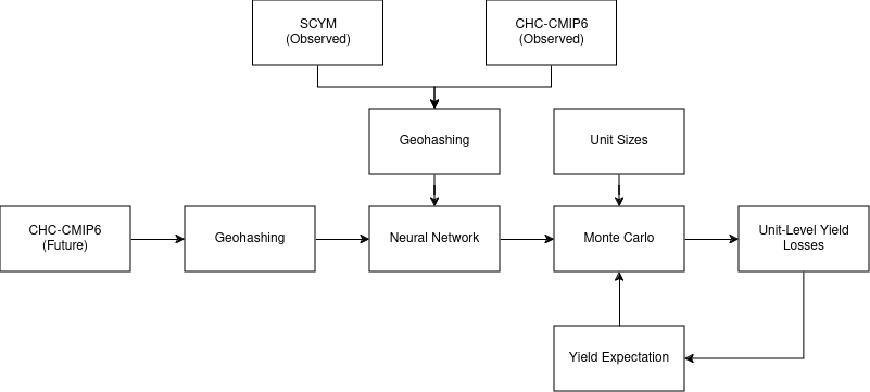
Figure 1: Model pipeline overview diagram. Code released as open source.

Note that, though offering predictions at 30 meter scale, SYCM uses Daymet variables at 1 km resolution (Thornton et al. 2014) and, thus, we more conservatively assume this 1km granularity in determining sample sizes.

2.5 Evaluation

We choose our model using each candidate’s capability to predict into future years, a “sweep temporal displacement” task representative of the Monte Carlo simulations (Brownlee 2020a):

• Train on all data between 1999 to 2012 inclusive.

• Use 2014 and 2016 as validation set to compare the 1,500 candidates.

• Test in which 2013 and 2015 serve as a fully hidden set in order to estimate how the chosen model may perform in the future.

Having performed model selection, we further evaluate our chosen regressor through three additional tests which more practically estimate performance in different ways one may consider using this method (see Table LABEL:tbl:posthoc) while using a larger training set.

Table 2: Overview of trials after model selection.

Trial	Purpose	Train	Test
Random Assignment	Evaluate ability to predict generally.	Random 75% of year / geohash combinations such that a geohash may be in training one year and test another.	The remaining 25% of year / region combinations.
Temporal Displacement	Evaluate ability to predict into future years.	All data from 1999 to 2013 inclusive.	All data 2014 to 2016 inclusive.
Spatial Displacement	Evaluate ability to predict into unseen geographic areas.	All 4 character geohashes in a randomly chosen 75% of 3 character regions.	Remaining 25% of regions.

These post-hoc trials use only training and test sets as we fully retrain models using unchanging sweep-chosen hyper-parameters. Note that some of these tests use “regions” which we define as all geohashes sharing the same first three characters. This two tier definition creates a grid of 109 x 156 km cells (Haugen 2020) each including all neighborhoods (4 character geohashes) found within that area.

3 Results

We project loss probabilities to more than double (5.5% claims rate) under SSP245 at mid-century in comparison to the no additional warming counterfactual scenario (1.9% claims rate).

3.1 Neural network outcomes

With bias towards performance in mean prediction, we select 4 layers (128 neurons, 64 neurons, 32 neurons, 8 neurons) using 0.01 dropout and 0.1 L2 from our sweep with all data attributes included. Table LABEL:tbl:sweep describes performance for the chosen configuration.

Table 3: Results of chosen configuration during the “sweep” for model selection.

Set	MAE for Mean Prediction	MAE for Std Prediction
Train	5.3%	1.6%
Validation	10.0%	4.0%
Test before retrain	12.4%	2.9%
Test after retrain	5.2%	1.9%

After retraining with train and validation together, we see 5.2% MAE when predicting neighborhood mean and 1.9% when predicting neighborhood standard deviation when using the fully hidden test set.

Next, having chosen this set of hyper-parameters, we also evaluate regression performance through varied definitions of test sets representing different tasks.

Table 4: Results of tests after model selection.

Task	Test Mean Pred MAE	Test Std Pred MAE	% of Units in Test Set
Temporal	6.3%	1.9%	17.0%
Spatial	5.5%	1.5%	25.0%
Random	5.1%	1.7%	19.1%

From the trials outlined in Table LABEL:tbl:posthocresults, the temporal task best resembles expected error in simulations as they predict into the future. The interactive tools website allows for further examination of error.

3.2 Simulation outcomes

After retraining on all available data using the selected configuration from our sweep, Monte Carlo simulates overall outcomes. Despite the conservative nature of the Bonferroni correction (McDonald 2014) and the 1km sample assumption, 91.1% of maize acreage in SSP245 falls within a neighborhood with significant changes to claim probability ($p<0.05/n$) at some point during the 2050 series simulations. That said, we observe that some of the remaining neighborhoods failing to meet that threshold have less land dedicated to maize within their area and, thus, a smaller sample size in our simulations.

Table 5: Overview of Monte Carlo simulation results. Counterfactual is a future without continued warming in contrast to SSP245.

Scenario	Year	Unit mean yield change	Unit loss probability	Avg covered loss severity
Counterfactual	2030	13.6%	1.6%	9.8%
SSP245	2030	4.9%	4.5%	10.3%
Counterfactual	2050	10.3%	1.9%	10.1%
SSP245	2050	0.5%	5.5%	10.8%
		$y_{\Delta\mu}$	$p_{\mu}$	$s_{\mu}$

Regardless, with Table LABEL:tbl:simresults highlighting these climate threats, these simulations suggest that warming disrupts historic trends of increasing average yield (Nielsen 2023).

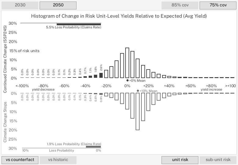
Figure 2: Interactive tool screenshot showing 2050 outcomes distribution (changes from $y_{expected}$), highlighting loss with and without climate change. In addition to showing increased claims rate, this also depicts climate change reducing the expected increase in yields that would otherwise follow historic trends.

Furthermore, in addition to wiping out the gains that our neural network would otherwise expect without climate change, the loss probability increases in both of the time frames considered for SSP245. Indeed, as shown in Figure 2, the SSP245 overall yield mean remains similar to the historic baseline even as distribution tails differ more substantially. This shows how a sharp increase in loss probability (2050 series vs counterfactual) could emerge without necessarily changing average yields.

4 Discussion

In addition to highlighting future work opportunities, we observe a number of policy-relevant dynamics within our simulations.

4.1 Adaptation and policy structure

Adaptation to these adverse conditions is imperative for both farmers and insurers (O’Connor and Bryant 2017; McBride et al. 2020.). In order to confront this alarming increase in climate-driven risk, preparations may include:

• Altering planting dates (Mangani, Gunn, and Creux 2023).

• Physically moving operations (Butler and Huybers 2013).

• Employing stress-resistant varieties (Tian et al. 2023).

• Modifying pesticide usage (Keronen et al. 2023).

• Adopting risk-mitigating regenerative farming systems (Renwick et al. 2021).

Most notably, regenerative practices can reduce risks through diverse crop rotations (Bowles et al. 2020) and improvements to soil health (Renwick et al. 2021). These important steps may provide output stability in addition to other environmental benefits (Hunt et al. 2020), valuable resilience given that our results see higher claims not through overall reduced averages but higher volatility. Still, significant structural and financial barriers inhibit adoption of such systems (McBride et al. 2020). In particular, though the magnitude remains the subject of empirical investigation (Connor, Rejesus, and Yasar 2022), financial safety net programs like crop insurance may reduce adoption (Wang, Rejesus, and Aglasan 2021; Chemeris, Liu, and Ker 2022) despite likely benefits for both farmers and insurers (O’Connor and Bryant 2017).

One specific feature of U.S. crop insurance policy may be partly responsible for this disincentive: average-based production histories (FCIC 2020) structurally reward increases in mean yield but not necessarily yield stability. Indeed, regenerative agricultural practices may not always improve mean yields or can even come at the cost of a slightly reduced average (Deines et al. 2023) even though they guard against elevations in the probability of loss events (Renwick et al. 2021).

That in mind, if coverage levels are redefined from the current percentage based approach ($l_{\%}$) to variance ($l_{\sigma}$) as shown in Table LABEL:tbl:covformula, then improvements both in average yield and stability could be rewarded. For example, using historic values as guide, 2.11 standard deviations ($c_{\sigma}$) would achieve the current system-wide coverage levels ($c_{\%}=0.75$) but realign incentives towards a balance between a long-standing aggregate output incentive and a new resilience reward that could recognize regenerative systems and other strategies that reduce variability, valuing the stability offered by some producers for the broader food system (Renwick et al. 2021).

Table 6: Change in coverage formulas.

Current formulation	Possible proposal
$l_{\%}=\max(c_{\%}*y_{\mu}-y_{acutal},0)$	$l_{\sigma}=\max(\frac{c_{\sigma}*y_{\mu}}{y_{\sigma}}-y_{acutal},0)$

Table 6 further describes this translation between standard deviation and historic coverage levels. Even so, federal statute may cap coverage levels as percentages of production history (CFR and USC, n.d.). Therefore, though regulators may make improvements like through 508h without congressional action, our simulations possibly suggest that the ability to incorporate climate adaptation variability may remain limited without statutory change.

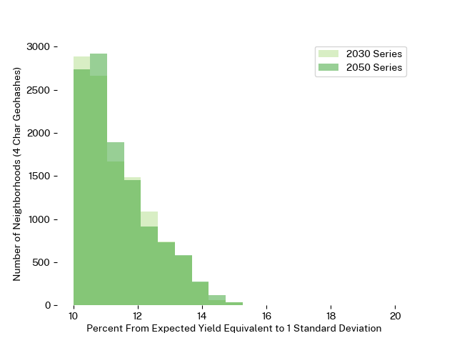
Figure 3: Histogram showing percent change from $y_{expected}$ for one standard deviation in each simulated unit.

Regardless, $l_{\sigma}$ enables rate setters to directly reward outcomes instead of individual practices and combining across management tools may address unintended consequences of elevating individual risk management options (Connor, Rejesus, and Yasar 2022). Though recognizing the limits of insurance alone and echoing prior calls for multi-modal support for regenerative systems (McBride et al. 2020), this outcomes-based approach may enable insurance to more directly support climate adaptation without picking specific systems or practices to incentivize.

4.2 Geographic bias

Neighborhoods with significant results ($p<0.05/n$) may be more common in some areas as shown in Figure 4. This spatial pattern may partially reflect that a number of neighborhoods have less land dedicated to maize so simulations have smaller sample sizes and fail to reach significance. In other cases, this geographic effect may also reflect disproportionate stress or other changes relative to historic conditions. In particular, as further explorable in our interactive tools, we note some geographic bias in changes to precipitation, temperature, and VPD / SVP.

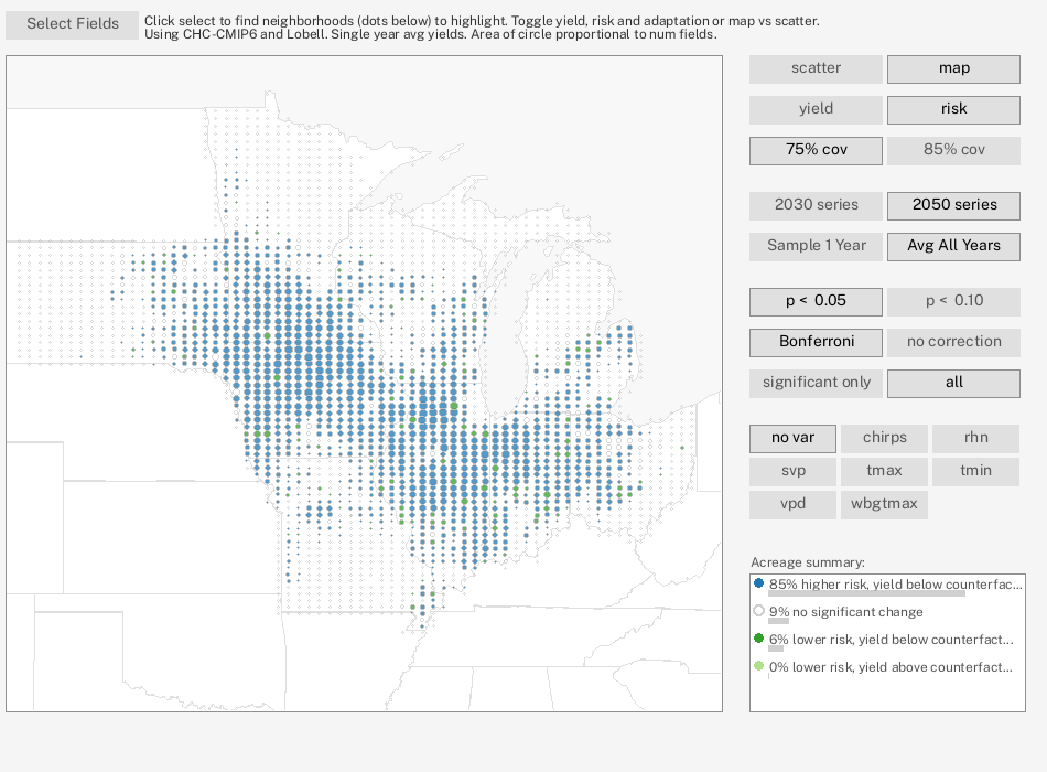
Figure 4: Interactive geographic view. Color describes type of change and larger dots are larger areas of maize growing activity. Band of increased risk concentrates in Iowa, Illinois, and Indiana.

4.3 Trend-adjustment

Nielsen (2023) suggests that historic trends would anticipate continued increases in maize outputs but our simulations predict climate change to wipe out the 10.3% yield increase that our neural network would otherwise expect within the counterfactual simulation without further warming. This flattening of yield increases may impact not just aggregate output but also how growers choose options such as trend adjustment (Plastina and Edwards 2014).

4.4 Heat and drought stress

Our model shows depressed yields during combined warmer and drier conditions, combinations similar to 2012 and its historically poor maize production (ERS 2013). In this context, precipitation may serve as a protective factor: neighborhoods with drier July conditions see higher loss probability ($p<0.05/2$) in both the 2030 and 2050 series via rank correlation (Spearman 1904). Our predictions thus reflect empirical studies that document the negative impacts of heat stress and water deficits on maize yields (Sinsawat et al. 2004; Marouf et al. 2013).

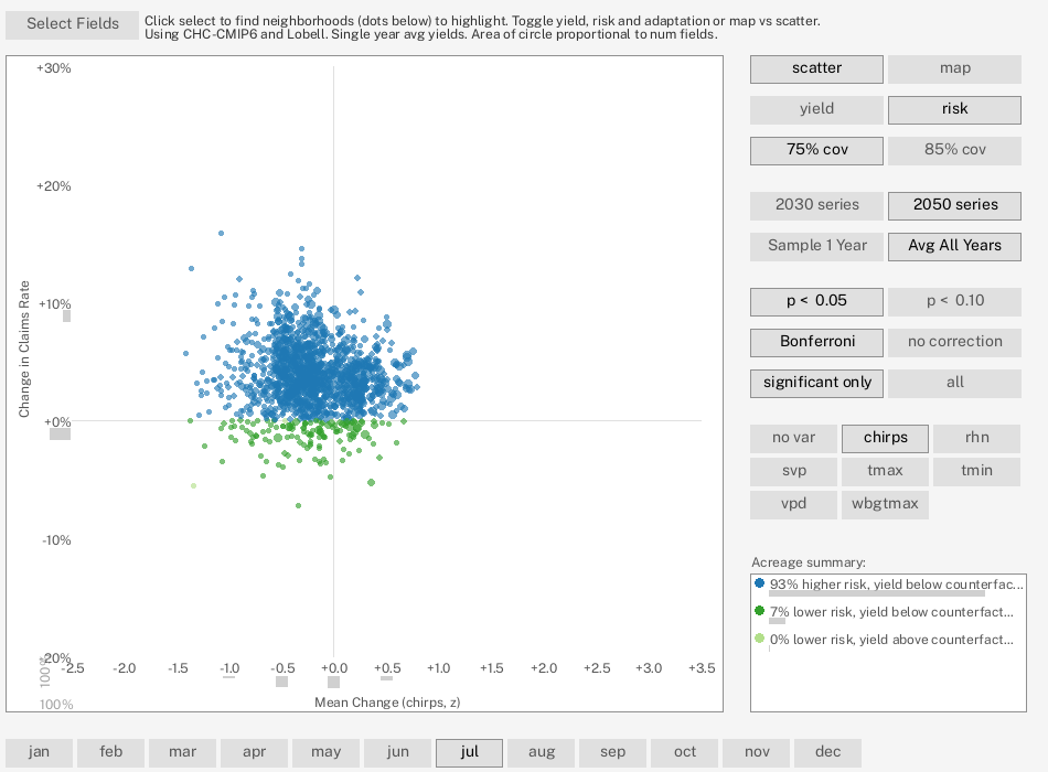
Figure 5: Screenshot of an interactive tool showing precipitation and loss probability changes. The horizontal axis is change in precipitation and the vertical axis is the change in claims rate (probability of covered loss).

These outputs may also reveal geographically and temporally specific outlines of these protective factors, possibly useful for insurer and grower adaptation. Even so, as pictured in Figure 5, we caution that analysis finds significant but weak rank correlations in both series, indicating that model expectations cannot be described by precipitation alone.

4.5 Risk unit size

Prior work expects larger insured units to reduce risk (Knight et al. 2010) and we similarly observe a claims rate decrease as the acreage included in an insured unit grows. As this structure may change in the future, we run post-hoc experiments altering unit size to determine robustness of our findings:

• Simulate outcomes as if units contain approximately single fields, decreasing aggregation.

• Simulate outcomes with removal of smaller Optional Units (Zulauf 2023), increasing aggregation.

In both cases, a gap persists in claims rates between the counterfactual and SSP245, suggesting concerns remain relevant even as unit sizes evolve.

4.6 Other models and programs

We also highlight additional future modeling opportunities beyond the scope of this study.

• We evaluate yield deltas and include historic yield as inputs into our neural network, allowing those data to “embed” adaptability measures (Hsiang et al. 2017) such as soil properties and practices. However, those estimating absolute yield prediction may consider Rayburn and Basden (2022) as well as Woodard and Verteramo-Chiu (2017) to incorporate other variables like soil properties.

• Later research may also extend to genetic modification and climate-motivated practice changes which we assume to be latent in historic data.

• Though our interactive tools consider alternatives to SCYM and different spatial aggregations such as 5 character (4 x 5 km) geohashes, future work may consider modeling with actual field-level yield data and the actual risk unit structure. To that end, we observe that the actual unit yields / revenue and risk unit structure are not currently public.

• Due to the robustness of yield data, we examine Yield Protection but future agroeconomic study could extend this to the highly related Revenue Protection (RP) form of insurance. Indeed, the yield stresses seen in YP that we describe in this model may also impact RP.

• With additional data, future modeling could relax our normality assumption though, in addition to 79% of neighborhoods seeing approximately normal yield deltas, we observe that 88% of neighborhoods see approximate symmetry per H.-Y. Kim (2013) so that later work would likely not remove a systemic directional bias in results.

Note that, while we do anticipate changing historic yield averages in our simulations, we take a conservative approach and do not consider trend adjustment (Plastina and Edwards 2014) and yield exclusion years (Schnitkey, Sherrick, and Coppess 2015). In raising $y_{expected}$, both would likely increase simulated loss rates.

4.7 Interactive tools

In order to explore these simulated distributions geographically and under different scenarios, interactive open source web-based visualizations built alongside our experiments both aid in constructing our own conclusions and allow readers to consider possibilities and analysis beyond our own narrative.

Table 7: Overview of explorable explanations.

Simulator	Question	Loop	JG
Rates	What factors influence the price and subsidy of a policy?	Iteratively change variables to increase subsidy.	Improving on previous hypotheses.
Hyper-Parameter	How do hyper-parameters impact regressor performance?	Iteratively change neural network hyper-parameters to see influence on validation set performance.	Improving on previous hyper-parameter hypotheses.
Distributional	How do overall simulation results change under different simulation parameters?	Iterative manipulation of parameters (geohash size, event threshold, year) to change loss probability and severity.	Deviating from the study’s main results.
Neighborhood	How do simulation results change across geography and climate conditions?	Inner loop changing simulation parameters to see changes in neighborhood outcomes. Outer loop of observing changes across different views.	Identifying neighborhood clusters of concern.
Claims	How do different regulatory choices influence grower behavior?	Iteratively change production history to see which years result in claims under different regulatory schemes.	Redefining policy to improve yield stability.

In crafting the “explorable explanations” (Victor 2011) in Table LABEL:tbl:apps, we draw analogies to micro-apps (Bridgwater 2015) or mini-games (DellaFave 2014) in which the user encounters a series of small experiences that, each with distinct interaction and objectives, can only provide minimal instruction (Brown 2024). As these visualizations cannot take advantage of design techniques like Hayashida-style tutorials (Pottinger and Zarpellon 2023), they rely on simple “loops” (Brazie 2024) for immediate “juxtaposition gratification” (JG) (JM8 2024), showing fast progression after minimal input.

Following Unwin (2020), our custom tools first serve as internal “exploratory” graphics enabling the insights detailed in our results with Table LABEL:tbl:insights outlining specific observations we attribute to our use of these tools.

Table 8: Observations we made from our own tools in the “exploratory” graphic context of Unwin (2020).

Simulator	Observation
Distributional	Dichotomy of larger changes to insurer-relevant tails contrasting smaller changes to mean yield.
Claims	Issues of using average for $y_{expected}$ (FCIC 2020).
Neighborhood	Eastward bias of impact. Model output relationships with broader climate factors, highlighting the possible systemic protective value of increased precipitation.
Hyper-parameter	Model resilience to removing individual inputs.

Then, continuing to “presentation” (Unwin 2020), we next release these tools into a open source website at https://ag-adaptation-study.pub.

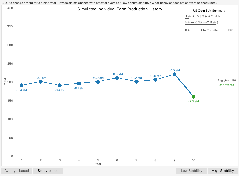
Figure 6: Example interactive showing how a high stability unit could see a claim for a bad year under $l_{\sigma}$ but not $l_{\%}$.

These public interactive visualizations allow for further exploration of our modeling such as different loss thresholds for other insurance products, finding relationships of outcomes to different climate variables, answering geographically specific questions beyond the scope of this study, and modification of machine learning parameters to understand performance. This may include use as workshop activity and we also report briefly on design changes made to our interactive tools in response to its participation in a 9 person “real-world” workshop session co-exploring these results:

• Like Pottinger et al. (2023), facilitatation alternates between presentation and interaction but, in response to a previously “lecture-heavy” initial background, we add the rates simulator to let facilitators break up that section.

• Facilitators suggest that single loop (Brazie 2024) designs perform best within the limited time of the workshop and we now let facilitators hold the longer two loop neighborhood simulator till the end by default.

• As expected by the JG design (JM8 2024), discussion contrasts different results sets and configurations of models but meta-parameter visualization relies heavily on memory so we now offer a “sweep” button for facilitators to show all results at once.

Later work may include controlled experimentation (Lewis 1982) or diary studies (Shneiderman and Plaisant 2006) for more generalizable design knowledge.

5 Conclusion

Maize production not only suffers from climate warming’s effects (Jägermeyr et al. 2021) but also adds to future climate change (Kumar et al. 2021). Inside this cyclic relationship, agriculture could crucially contribute to the necessary solution for the same global crisis that ails it (Schön, Gentsch, and Breunig 2024). In dialogue with prior work (Wang, Rejesus, and Aglasan 2021; Chemeris, Liu, and Ker 2022), we highlight how existing policy currently prioritizes increased mean yield over climate adaptations benefiting stability. Furthermore, we demonstrate how current structures could fail to adjust to our predicted distributional changes and how inclusion of variance into those regulatory structures may positively influence adoption of mitigating practices such as regenerative systems. This responsive shift in coverage levels could reorient incentives: balancing overall yield with longitudinal stability and more comprehensively incorporating an understanding of risk. These resilience-promoting changes may benefit both grower and insurer without requiring practice-specific regulation. Recognizing that these structural levers require modification by policy makers, we therefore encourage scientists to further study, regulators / lawmakers to further consider, and producers to further inform these revisions. These essential multi-stakeholder efforts are crucial in preparing the US food system and its insurance program for a warmer future.

6 Acknowledgements

Study funded by the Eric and Wendy Schmidt Center for Data Science and Environment at the University of California, Berkeley. We have no conflicts of interest to disclose. Using yield estimation data from Lobell et al. (2015) and Deines et al. (2021) with our thanks to David Lobell for permission. We also wish to thank Magali de Bruyn, Nick Gondek, Jiajie Kong, Kevin Koy, and Ciera Martinez for conversation regarding these results. Thanks to Color Brewer (Brewer et al. 2013) and Public Sans (General Services Administration 2024).

Works Cited

References

- Ates, Aaron. 2023. “Feed Grains Sector at a Glance.” Economic Research Service, USDA. https://www.ers.usda.gov/topics/crops/corn-and-other-feed-grains/feed-grains-sector-at-a-glance/.
- Baheti, Pragati. 2021. “The Essential Guide to Neural Network Architectures.” V7Labs. https://www.v7labs.com/blog/neural-network-architectures-guide.
- Bonferroni, Carlo. 1935. “Il Calcolo Delle Assicurazioni Su Gruppi Di Teste.” Studi in Onore Del Professore Salvatore Ortu Carboni. https://www.semanticscholar.org/paper/Il-calcolo-delle-assicurazioni-su-gruppi-di-teste-Bonferroni-Bonferroni/98da9d46e4c442945bfd88db72be177e7a198fd3.
- Bowles, Timothy M., Maria Mooshammer, Yvonne Socolar, Francisco Calderón, Michel A. Cavigelli, Steve W. Culman, William Deen, et al. 2020. “Long-Term Evidence Shows That Crop-Rotation Diversification Increases Agricultural Resilience to Adverse Growing Conditions in North America.” One Earth 2 (3): 284–93. https://doi.org/10.1016/j.oneear.2020.02.007.
- Brazie, Alexander. 2024. “Designing the Core Gameplay Loop: A Beginner’s Guide.” Game Design Skills. https://gamedesignskills.com/game-design/core-loops-in-gameplay/.
- Brewer, Cynthia, Mark Harrower, Ben Sheesley, Andy Woodruff, and David Heyman. 2013. “ColorBrewer 2.0.” The Pennsylvania State University.
- Bridgwater, Adrian. 2015. “What Are ’Micro Apps’ – and Why Do They Matter for Mobile?” Forbes. https://www.forbes.com/sites/adrianbridgwater/2015/07/16/what-are-micro-apps-and-why-do-they-matter-for-mobile/.
- Brown, Mark. 2024. “The 100 Games That Taught Me Game Design.” Game Maker’s Toolkit. https://www.youtube.com/watch?v=gWNXGfXOrro.
- Brownlee, Jason. 2020a. “What Is the Difference Between Test and Validation Datasets?” Guiding Tech Media. https://machinelearningmastery.com/difference-test-validation-datasets/.
- ———. 2020b. “Deep Learning Models for Multi-Output Regression.” Guiding Tech Media. https://machinelearningmastery.com/deep-learning-models-for-multi-output-regression/.
- Butler, Ethan E., and Peter Huybers. 2013. “Adaptation of US Maize to Temperature Variations.” Nature Climate Change 3 (1): 68–72. https://doi.org/10.1038/nclimate1585.
- CFR, and USC. n.d. Crop Insurance. https://uscode.house.gov/view.xhtml?req=(title:7%20section:1508%20edition:prelim).
- Chemeris, Anna, Yong Liu, and Alan P. Ker. 2022. “Insurance Subsidies, Climate Change, and Innovation: Implications for Crop Yield Resiliency.” Food Policy 108 (April): 102232. https://doi.org/10.1016/j.foodpol.2022.102232.
- Chite, Ralph. 2006. “Agricultural Issues in the 110th Congress.” Congressional Research Service. https://www.policyarchive.org/download/4403.
- Connor, Lawson, Roderick M. Rejesus, and Mahmut Yasar. 2022. “Crop Insurance Participation and Cover Crop Use: Evidence from Indiana County-level Data.” Applied Economic Perspectives and Policy 44 (4): 2181–2208. https://doi.org/10.1002/aepp.13206.
- Dai, Aiguo. 2013. “Increasing Drought Under Global Warming in Observations and Models.” Nature Climate Change 3 (1): 52–58. https://doi.org/10.1038/nclimate1633.
- Deines, Jillian M., Kaiyu Guan, Bruno Lopez, Qu Zhou, Cambria S. White, Sheng Wang, and David B. Lobell. 2023. “Recent Cover Crop Adoption Is Associated with Small Maize and Soybean Yield Losses in the United States.” Global Change Biology 29 (3): 794–807. https://doi.org/10.1111/gcb.16489.
- Deines, Jillian M., Rinkal Patel, Sang-Zi Liang, Walter Dado, and David B. Lobell. 2021. “A Million Kernels of Truth: Insights into Scalable Satellite Maize Yield Mapping and Yield Gap Analysis from an Extensive Ground Dataset in the US Corn Belt.” Remote Sensing of Environment 253 (February): 112174. https://doi.org/10.1016/j.rse.2020.112174.
- DellaFave, Robert. 2014. “Designing RPG Mini-Games (and Getting Them Right).” https://www.gamedeveloper.com/design/designing-rpg-mini-games-and-getting-them-right-.
- Diffenbaugh, Noah S, Frances V Davenport, and Marshall Burke. 2021. “Historical Warming Has Increased u.s. Crop Insurance Losses.” Environmental Research Letters 16 (8): 084025. https://doi.org/10.1088/1748-9326/ac1223.
- ERS. 2013. “Weather Effects on Expected Corn and Soybean Yield.” United States Department of Agriculture. https://www.ers.usda.gov/webdocs/outlooks/36651/39297_fds-13g-01.pdf?v=737.
- FCIC. 2020. “Common Crop Insurance Policy 21.1-BR.” United States Department of Agriculture. https://www.rma.usda.gov/-/media/RMA/Publications/Risk-Management-Publications/rma_glossary.ashx?la=en.
- ———. 2023. “Crop Insurance Handbook: 2024 and Succeeding Crop Years.” United States Department of Agriculture. https://www.rma.usda.gov/-/media/RMA/Handbooks/Coverage-Plans---18000/Crop-Insurance-Handbook---18010/2024-18010-1-Crop-Insurance-Handbook.ashx.
- General Services Administration. 2024. “Public Sans.” General Services Administration. https://public-sans.digital.gov/.
- Hanrahan, Ryan. 2024. “Crop Insurance Costs Projected to Jump 29%.” University of Illinois. https://farmpolicynews.illinois.edu/2024/02/crop-insurance-costs-projected-to-jump-29/.
- Haugen, Blake. 2020. “Geohash Size Variation by Latitude.” https://bhaugen.com/blog/geohash-sizes/.
- Hausfather, Zeke, and Glen Peters. 2020. “Emissions – the ‘Business as Usual’ Story Is Misleading.” Nature. https://www.nature.com/articles/d41586-020-00177-3.
- Hsiang, Solomon, Robert Kopp, Amir Jina, James Rising, Michael Delgado, Shashank Mohan, D. J. Rasmussen, et al. 2017. “Estimating Economic Damage from Climate Change in the United States.” Science 356 (6345): 1362–69. https://doi.org/10.1126/science.aal4369.
- Hunt, Natalie D., Matt Liebman, Sumil K. Thakrar, and Jason D. Hill. 2020. “Fossil Energy Use, Climate Change Impacts, and Air Quality-Related Human Health Damages of Conventional and Diversified Cropping Systems in Iowa, USA.” Environmental Science & Technology 54 (18): 11002–14. https://doi.org/10.1021/acs.est.9b06929.
- Jägermeyr, Jonas, Christoph Müller, Alex C. Ruane, Joshua Elliott, Juraj Balkovic, Oscar Castillo, Babacar Faye, et al. 2021. “Climate Impacts on Global Agriculture Emerge Earlier in New Generation of Climate and Crop Models.” Nature Food 2 (11): 873–85. https://doi.org/10.1038/s43016-021-00400-y.
- JM8. 2024. “The Secret to Making Any Game Satisfying | Design Delve.” Second Wind Group. https://www.youtube.com/watch?v=ORsb7g_ioLs.
- Joseph, Rohan. 2018. “Grid Search for Model Tuning.” Towards Data Science. https://towardsdatascience.com/grid-search-for-model-tuning-3319b259367e.
- Keronen, Sanna, Marjo Helander, Kari Saikkonen, and Benjamin Fuchs. 2023. “Management Practice and Soil Properties Affect Plant Productivity and Root Biomass in Endophyte-symbiotic and Endophyte-free Meadow Fescue Grasses.” Journal of Sustainable Agriculture and Environment 2 (1): 16–25. https://doi.org/10.1002/sae2.12035.
- Kim, Hae-Young. 2013. “Statistical Notes for Clinical Researchers: Assessing Normal Distribution (2) Using Skewness and Kurtosis.” Restorative Dentistry & Endodontics 38 (1): 52. https://doi.org/10.5395/rde.2013.38.1.52.
- Kim, Yang-Seon, Moon Keun Kim, Nuodi Fu, Jiying Liu, Junqi Wang, and Jelena Srebric. 2024. “Investigating the Impact of Data Normalization Methods on Predicting Electricity Consumption in a Building Using Different Artificial Neural Network Models.” Sustainable Cities and Society, June, 105570. https://doi.org/10.1016/j.scs.2024.105570.
- Kingma, Diederik P., and Jimmy Ba. 2014. “Adam: A Method for Stochastic Optimization.” https://doi.org/10.48550/ARXIV.1412.6980.
- Knight, Thomas O., Keith H. Coble, Barry K. Goodwin, Roderick M. Rejesus, and Sangtaek Seo. 2010. “Developing Variable Unit-Structure Premium Rate Differentials in Crop Insurance.” American Journal of Agricultural Economics 92 (1): 141–51. http://www.jstor.org/stable/40647972.
- Kumar, Rakesh, S. Karmakar, Asisan Minz, Jitendra Singh, Abhay Kumar, and Arvind Kumar. 2021. “Assessment of Greenhouse Gases Emission in Maize-Wheat Cropping System Under Varied n Fertilizer Application Using Cool Farm Tool.” Frontiers in Environmental Science 9 (September): 710108. https://doi.org/10.3389/fenvs.2021.710108.
- Kwiatkowski, Robert. 2022. “Monte Carlo Simulation — a Practical Guide.” https://towardsdatascience.com/monte-carlo-simulation-a-practical-guide-85da45597f0e.
- Leng, Guoyong, and Jim W Hall. 2020. “Predicting Spatial and Temporal Variability in Crop Yields: An Inter-Comparison of Machine Learning, Regression and Process-Based Models.” Environmental Research Letters 15 (4): 044027. https://doi.org/10.1088/1748-9326/ab7b24.
- Lewis, Clayton. 1982. “Using the "Thinking-Aloud" Method in Cognitive Interface Design.” IBM Research. https://dominoweb.draco.res.ibm.com/2513e349e05372cc852574ec0051eea4.html.
- Li, Kuo, Jie Pan, Wei Xiong, Wei Xie, and Tariq Ali. 2022. “The Impact of 1.5 °c and 2.0 °c Global Warming on Global Maize Production and Trade.” Scientific Reports 12 (1): 17268. https://doi.org/10.1038/s41598-022-22228-7.
- Lobell, David B., Jillian M. Deines, and Stefania Di Tommaso. 2020. “Changes in the Drought Sensitivity of US Maize Yields.” Nature Food 1 (11): 729–35. https://doi.org/10.1038/s43016-020-00165-w.
- Lobell, David B., David Thau, Christopher Seifert, Eric Engle, and Bertis Little. 2015. “A Scalable Satellite-Based Crop Yield Mapper.” Remote Sensing of Environment 164 (July): 324–33. https://doi.org/10.1016/j.rse.2015.04.021.
- Loshchilov, Ilya, and Frank Hutter. 2017. “Decoupled Weight Decay Regularization.” In International Conference on Learning Representations. https://api.semanticscholar.org/CorpusID:53592270.
- Maas, Andrew, Awni Hannun, and Andrew Ng. 2013. “Rectifier Nonlinearities Improve Neural Network Acoustic Models.” In Proceedings of the 30th International Conference on Machine Learning. Vol. 28. Atlanta, Georgia: JMLR.
- Mangani, Robert, Kpoti M. Gunn, and Nicky M. Creux. 2023. “Projecting the Effect of Climate Change on Planting Date and Cultivar Choice for South African Dryland Maize Production.” Agricultural and Forest Meteorology 341 (October): 109695. https://doi.org/10.1016/j.agrformet.2023.109695.
- Mann, H. B., and D. R. Whitney. 1947. “On a Test of Whether One of Two Random Variables Is Stochastically Larger Than the Other.” The Annals of Mathematical Statistics 18 (1): 50–60. https://doi.org/10.1214/aoms/1177730491.
- Manski, Sarah, Yvonne Socolar, Ben Goldstein, Gina Pizzo, Zobaer Ahmed, Lawson Connor, Harley Cross, et al. 2024. “Diversified Crop Rotations Mitigate Agricultural Losses from Dry Weather.” agriRxiv, April, 20240168962. https://doi.org/10.31220/agriRxiv.2024.00244.
- Marouf, Khalily, Mohammad Naghavi, Alireza Pour-Aboughadareh, and Houshang Naseri rad. 2013. “Effects of Drought Stress on Yield and Yield Components in Maize Cultivars (Zea Mays l).” International Journal of Agronomy and Plant Production 4 (January): 809–12.
- McBride, Fiona, Ethan Elkind, Nina Ichikawa, and Ken Alex. 2020. “Redefining Value and Risk in Agriculture.” https://food.berkeley.edu/wp-content/uploads/2020/12/BFI_ValueRisk_in_Ag_120920_Digital.pdf.
- McDonald, J. H. 2014. Handbook of Biological Statistics. 3rd ed. Baltimore, Maryland: Sparky House Publishing. http://www.biostathandbook.com/#print.
- Metropolis, Nick. 1987. “The Beginning of the Monte Carlo Method.” Los Alamos Science. https://sgp.fas.org/othergov/doe/lanl/pubs/00326866.pdf.
- Mwiti, Derrick. 2023. “Random Forest Regression: When Does It Fail and Why?” Neptune.ai. https://neptune.ai/blog/random-forest-regression-when-does-it-fail-and-why.
- Nielsen, R. L. 2023. “Historical Corn Grain Yields in the u.s.” Purdue University. https://www.agry.purdue.edu/ext/corn/news/timeless/yieldtrends.html.
- Niemeyer, Gustavo. 2008. “Geohash.org Is Public!” Labix Blog. https://web.archive.org/web/20080305102941/http://blog.labix.org/2008/02/26/geohashorg-is-public/.
- O’Connor, Claire, and Lara Bryant. 2017. “Covering Crops: How Federal Crop Insurance Program Reforms Can Reduce Costs, Empower Farmers, and Protect Natural Resources.” National Resources Defense Council. https://www.nrdc.org/sites/default/files/federal-crop-insurance-program-reforms-ip.pdf.
- Plastina, Alejandro, and William Edwards. 2014. “Trend-Adjusted Actual Production History (APH).” Iowa State University Extension; Outreach. https://www.extension.iastate.edu/agdm/crops/html/a1-56.html.
- Pottinger, A Samuel, Nivedita Biyani, Roland Geyer, Douglas J McCauley, Magali de Bruyn, Molly R Morse, Neil Nathan, Kevin Koy, and Ciera Martinez. 2023. “Combining Game Design and Data Visualization to Inform Plastics Policy: Fostering Collaboration Between Science, Decision-Makers, and Artificial Intelligence.” https://doi.org/10.48550/ARXIV.2312.11359.
- Pottinger, A Samuel, and Giulia Zarpellon. 2023. “Pyafscgap.org: Open Source Multi-Modal Python-Basedtools for NOAA AFSC RACE GAP.” Journal of Open Source Software 8 (86): 5593. https://doi.org/10.21105/joss.05593.
- Ray, Deepak K., James S. Gerber, Graham K. MacDonald, and Paul C. West. 2015. “Climate Variation Explains a Third of Global Crop Yield Variability.” Nature Communications 6 (1): 5989. https://doi.org/10.1038/ncomms6989.
- Rayburn, Edward B., and Tom Basden. 2022. “Comparison of Crop Yield Estimates Obtained from an Historic Expert System to the Physical Characteristics of the Soil Components—a Project Report.” Agronomy 12 (4): 765. https://doi.org/10.3390/agronomy12040765.
- Renwick, Leah L R, William Deen, Lucas Silva, Matthew E Gilbert, Toby Maxwell, Timothy M Bowles, and Amélie C M Gaudin. 2021. “Long-Term Crop Rotation Diversification Enhances Maize Drought Resistance Through Soil Organic Matter.” Environmental Research Letters 16 (8): 084067. https://doi.org/10.1088/1748-9326/ac1468.
- Rezaei, Ehsan Eyshi, Heidi Webber, Senthold Asseng, Kenneth Boote, Jean Louis Durand, Frank Ewert, Pierre Martre, and Dilys Sefakor MacCarthy. 2023. “Climate Change Impacts on Crop Yields.” Nature Reviews Earth & Environment 4 (12): 831–46. https://doi.org/10.1038/s43017-023-00491-0.
- RMA. 2008. “Crop Insurance Options for Vegetable Growers.” https://www.rma.usda.gov/-/media/RMA/Publications/Risk-Management-Publications/vegetable_growers.ashx?la=en.
- ———. 2024. “State/County/Crop Summary of Business.” United States Department of Agriculture. https://www.rma.usda.gov/SummaryOfBusiness/StateCountyCrop.
- Sajid, Osama, Ariel Ortiz-Bobea, Jennifer Ifft, and Vincent Gauthier. 2023. “Extreme Heat and Kansas Farm Income.” Farmdoc Daily of Department of Agricultural; Consumer Economics, University of Illinois at Urbana-Champaign. https://farmdocdaily.illinois.edu/2023/07/extreme-heat-and-kansas-farm-income.html.
- Schechinger, Anne. 2023. “Crop Insurance Costs Soar over Time, Reaching a Record High in 2022.” Environmental Working Group. https://www.ewg.org/research/crop-insurance-costs-soar-over-time-reaching-record-high-2022.
- Schnitkey, Gary, Bruce Sherrick, and Jonathan Coppess. 2015. “Yield Exclusion: Description and Guidance.” Department of Agricultural; Consumer Economics, University of Illinois at Urbana-Champaign. https://origin.farmdocdaily.illinois.edu/2015/01/yield-exclusion-description-and-guidance.html.
- Schön, Jonas, Norman Gentsch, and Peter Breunig. 2024. “Cover Crops Support the Climate Change Mitigation Potential of Agroecosystems.” Edited by Abhay Omprakash Shirale. PLOS ONE 19 (5): e0302139. https://doi.org/10.1371/journal.pone.0302139.
- Shneiderman, Ben, and Catherine Plaisant. 2006. “Strategies for Evaluating Information Visualization Tools: Multi-Dimensional in-Depth Long-Term Case Studies.” In Proceedings of the 2006 AVI Workshop on BEyond Time and Errors: Novel Evaluation Methods for Information Visualization, 1–7. Venice Italy: ACM. https://doi.org/10.1145/1168149.1168158.
- Sinsawat, Veerana, Jörg Leipner, Peter Stamp, and Yvan Fracheboud. 2004. “Effect of Heat Stress on the Photosynthetic Apparatus in Maize (Zea Mays l.) Grown at Control or High Temperature.” Environmental and Experimental Botany 52 (2): 123–29. https://doi.org/10.1016/j.envexpbot.2004.01.010.
- Spearman, C. 1904. “The Proof and Measurement of Association Between Two Things.” The American Journal of Psychology 15 (1): 72. https://doi.org/10.2307/1412159.
- Thornton, P. E., M. M. Thornton, B. W. Mayer, N. Wilhelmi, Y. Wei, R. Devarakonda, and R. B. Cook. 2014. “Daymet: Daily Surface Weather Data on a 1-Km Grid for North America, Version 2.” ORNL Distributed Active Archive Center. https://doi.org/10.3334/ORNLDAAC/1219.
- Tian, Tian, Shuhui Wang, Shiping Yang, Zhirui Yang, Shengxue Liu, Yijie Wang, Huajian Gao, et al. 2023. “Genome Assembly and Genetic Dissection of a Prominent Drought-Resistant Maize Germplasm.” Nature Genetics 55 (3): 496–506. https://doi.org/10.1038/s41588-023-01297-y.
- Tsiboe, Francis, and Dylan Turner. 2023. “Crop Insurance at a Glance.” Economic Research Service, USDA. https://www.ers.usda.gov/topics/farm-practices-management/risk-management/crop-insurance-at-a-glance/.
- Unwin, Anthony. 2020. “Why Is Data Visualization Important? What Is Important in Data Visualization?” Harvard Data Science Review, January. https://doi.org/10.1162/99608f92.8ae4d525.
- Victor, Bret. 2011. “Explorable Explanations.” Bret Victor. http://worrydream.com/ExplorableExplanations/.
- Wang, Ruixue, Roderick M Rejesus, and Serkan Aglasan. 2021. “Warming Temperatures, Yield Risk and Crop Insurance Participation.” European Review of Agricultural Economics 48 (5): 1109–31. https://doi.org/10.1093/erae/jbab034.
- Williams, Emily, Chris Funk, Pete Peterson, and Cascade Tuholske. 2024. “High Resolution Climate Change Observations and Projections for the Evaluation of Heat-Related Extremes.” Scientific Data 11 (1): 261. https://doi.org/10.1038/s41597-024-03074-w.
- Woodard, Joshua D., and Leslie J. Verteramo-Chiu. 2017. “Efficiency Impacts of Utilizing Soil Data in the Pricing of the Federal Crop Insurance Program.” American Journal of Agricultural Economics 99 (3): 757–72. https://doi.org/10.1093/ajae/aaw099.
- Yanai, Ruth D., John J. Battles, Andrew D. Richardson, Corrie A. Blodgett, Dustin M. Wood, and Edward B. Rastetter. 2010. “Estimating Uncertainty in Ecosystem Budget Calculations.” Ecosystems 13 (2): 239–48. https://doi.org/10.1007/s10021-010-9315-8.
- Zulauf, Carl. 2023. “The Importance of Insurance Unit in Crop Insurance Policy Debates.” University of Illinois. https://farmdocdaily.illinois.edu/2023/06/the-importance-of-insurance-unit-in-crop-insurance-policy-debates.html.