An efficient strategy for path planning with a tethered marsupial robotics system

Abstract

A marsupial robotics system comprises three components: an Unmanned Ground Vehicle (UGV), an Unmanned Aerial Vehicle (UAV), and a tether connecting both robots. Marsupial systems are highly beneficial in industry as they extend the UAV’s battery life during flight. This paper introduces a novel strategy for a specific path planning problem in marsupial systems, where each of the components must avoid collisions with ground and aerial obstacles modeled as 3D cuboids. Given an initial configuration in which the UAV is positioned atop the UGV, the goal is to reach an aerial target with the UAV. We assume that the UGV first moves to a position from which the UAV can take off and fly through a vertical plane to reach an aerial target. We propose an approach that discretizes the space to approximate an optimal solution, minimizing the sum of the lengths of the ground and air paths. First, we assume a taut tether and use a novel algorithm that leverages the convexity of the tether and the geometry of obstacles to efficiently determine the locus of feasible take-off points for the UAV. We then apply this result to scenarios that involve loose tethers. The simulation test results show that our approach can solve complex situations in seconds, outperforming a baseline planning algorithm based on RRT* (Rapidly exploring Random Trees).

I Introduction

Multi-robot teams are helpful to carry out tasks in confined, harsh environments that may be harmful to humans. Robots can navigate to difficult access points and mitigate the exposure of human first-responders in applications like search&rescue [30, 3], sewer inspection [1], or inspection and mapping in abandoned mines [31]. The use of heterogeneous systems that integrate Unmanned Aerial Vehicles (UAVs) and Unmanned Ground Vehicles (UGVs) is an interesting option to combine the better maneuverability of UAVs with the higher payload capacity and battery autonomy of UGVs. In this work, we focus on marsupial systems [13], which are teams of robots with heterogeneous capabilities, where some act as providers to others. Typically, the provider deploys other robots and serves as a communication relay and/or recharge station. We are interested in tethered marsupial systems; in particular, a system operating in a confined space where a UGV deploys a tethered UAV to extend the autonomy of the latter through the cable.

Planning 3D collision-free paths for the operation of such tethered marsupial systems in confined scenarios is challenging in several manners. First, due to the high-dimensionality of the configuration space, as both robots present different locomotion capabilities and their motion needs to be planned in a coordinated manner. Second, the fact that the movement of both robots is coupled by a tether imposes additional constraints. Not only does the length of the tether have to be considered when planning paths, but also its shape to ensure that there are no cable entanglements or collisions, particularly in cluttered environments.

In this paper, we propose a method for 3D collision-free path planning of a marsupial system composed of a UGV that deploys a tethered UAV. We follow a sequential strategy for robot navigation: given a starting point of the marsupial system and a destination point to be visited by the UAV, we assume that the UGV will move first carrying the UAV to a location from where the final destination is accessible by the tethered UAV. The UAV is allowed to fly in a 2D vertical plane from above the UGV to the target. For that, we introduce a catenary-visibility problem where we search for candidate locations from where the UGV can deploy the UAV without colliding. We then compute a 2D path for the UAV starting at the candidate point that minimizes the time to reach the aerial target. We call our strategy MASPA, which stands for MArsupial Sequential Path-planning Approach.

When approaching the catenary-visibility problem, we assume that the tether is controllable and bounded by a maximum length $L$. We first study the case where the tether is taut and forms a polygonal chain, simulating a cable that is tangent to an arbitrary number of obstacles. In that case, we take advantage of the geometric properties of the problem and propose an $O(n^{2})$ time algorithm to find the exact locus of take-off points in a vertical plane from where the UAV can be deployed and reach the target (2D visibility). This algorithm allows us to construct a linear structure that avoids time-consuming queries about the existence of collision-free catenaries. Then, we extend the algorithm to approximate the locus of feasible take-off points in the space (3D visibility). We call the 3D version of the algorithm PVA after Polygonal Visibility Algorithm and use it as a key component in the MASPA strategy. In addition, we consider the case where the loose tether is realistically modeled as a catenary curve. We demonstrate that PVA can significantly reduce the search time for viable loose tethers, which is crucial in emergency scenarios.

I-A Related Work

The Multi-Robot Path Planning (MRPP) problem consists of computing collision-free paths for multiple robots from start locations to goal locations, minimizing different objectives based on covered distance or arrival time.

Numerous methods for robot path planning assume that the environment can be modeled by a graph and then compute optimal paths using graph search algorithms like Djikstra, A^⋆, or Theta* [27]. Probabilistic planners [11], such as Probabilistic Road-Maps (PRM) or Rapidly-exploring Random Trees (RRT), are also a widespread approach. Instead of considering a fully connected scenario, they build a graph by randomly sampling the environment, which makes them suitable for planning in high-dimensional spaces in reasonable computation time. Some variants, such as RRT^⋆ [15], can achieve optimal solutions asymptotically. Recently, reinforcement learning methods have also been applied to UAV navigation in complex environments [39], even considering a load hanging from a cable [12] or multi-agent teams [33].

In the multi-robot case, there are multiple works in the planning community for MRPP. Reduction-based methods try to reduce the path planning problem to other well-studied problems, such as integer linear programming [46, 40]; while search-based methods [34, 21] look for optimal paths by means of different strategies to explore the solution space. In decoupled search-based methods, robots plan their paths sequentially in some order of priority [41, 20]. Some of these methods for MRPP consider temporal [40] or kinematic constraints [21] for robots.

Additionally, MRPP can be modeled as a non-convex constrained optimization problem in 3D [2], and numerical methods can be used to find optimal solutions. For instance, Sequential Convex Programming has been proposed to obtain solutions in this non-convex optimization [9], or polyhedra representations of the robot trajectories in multi-UAV scenarios [37]. Another constrained optimization alternative for MRPP is Non-linear Model Predictive Control, where a receding time horizon approach is used to compute collision-free trajectories for multiple robots [47, 18].

More specifically, this work focuses on path planning for marsupial multi-robot systems that combine ground and aerial robots connected by a tether [26]. Dinelli et al. [10] wrote a review of UGV-UAV robotic systems for operation in underground rescue missions. Hierarchical trajectory generation has been proposed for marsupial robot systems [35], combining high-level multi-robot path planning on a topological graph that encodes the locomotion capabilities of each robot, with low-level dynamically feasible trajectory planning through RRT and non-linear programming. Although they plan trajectories that take into account the whole marsupial team in a coordinated manner, no specific constraints related to tethered systems are considered.

Sandino et al. [32] discuss the problem of landing a helicopter when GPS sensors are not reliable. In this case, using a tether connecting the helicopter to the base allows for the estimation of its linear position relative to the landing point. Moreover, the tension exerted on the tether provides a stabilizing effect on the helicopter’s translational dynamics. However, attached UAVs impose additional complexities in addressing cable disturbances in the robot controller [36] and avoiding cable entanglement [8]. Viegas et al. [38] presented a novel lightweight tethered UAV with mixed multi-rotor and water jet propulsion for forest fire fighting. The planning of tether-aware kinodynamic trajectories in formations with multiple tethered UAVs has also been considered [6, 8]. Nevertheless, these works assume that ground stations are static. There are also works on tethered UAV-UGV marsupial systems, with moving ground stations. A sensor system that measures the catenary shape of the cable can be used for relative localization [7]. Miki et al. [25] presented a cooperative tethered UAV-UGV system where the UAV can anchor the tether on top of a cliff to help the UGV climb, using a grid-based heuristic planner (A^⋆) for navigation. Furthermore, a hierarchical path planning approach with two independent RRT^⋆ has been proposed [28] for map generation missions. The UGV first plans its route and then the UAV limits its range according to the UGV plan and the tether length. Both methods approach motion planning independently for each robot, neglecting collision avoidance for the tether. In the work by Xiao et al. [42], given a fixed position of the UGV, the UAV follows the path using motion controllers that consider the relative angles and length of the tether. However, the joint UAV-UGV path planning problem is not addressed either. The same authors extended their previous work to build a marsupial robot system for search&rescue operation [44], with a teleoperated ground robot and an autonomous tethered UAV that provides visual feedback and situational awareness to the teleoperator. They implemented a probabilistic model for risk-aware path planning and even planned contact points of the tether with the environment to extend the UAV line of sight.

Despite these efforts in path planning and trajectory optimization for tethered marsupial systems [42, 44, 29, 19], all these previous works either do not include the tether in the UAV linear motion, or assume straight line or general taut tethers. They also assume that the UGV is fixed in a static position on the ground.

In a setting close to ours, Martinez-Rozas et al. [23] applied RRT^∗ and non-linear optimization based on sparse factored graphs to compute collision-free trajectories for a marsupial system with a UGV, a UAV, and a non-taut tether with controllable length. They consider a realistic model of the tether shape for collision checking, but the UGV is assumed to be static for trajectory planning.

The use of a setup where the UGV carries the UAV was justified by Nicolas Hudson et al. [14]. The authors used this setup in a challenge of subterranian exploration. A tethered UAV has also been used for the inspection of underground stone mine pillars [22]. The UAV stays landed on the UGV while the ensemble moves inside a mine. The mission of the UAV is to create 3D maps of the mine pillars to support time-lapse hazard mapping and time-dependent pillar degradation analysis.

I-B Contribution

Overall, optimal methods for MRPP suffer from scalability, and many try to alleviate the complexity of the problem by proposing hierarchical approaches or decoupled planning for robots. In our tethered marsupial system operating in 3D, due to the coupled nature of the motion, path planning needs to be performed in a high-dimensional configuration space that takes into account both robots. Therefore, there is a need for an efficient method capable of jointly computing optimal robot paths in a reasonable time. Furthermore, most existing MRPP methods do not consider the specific constraints imposed by a tether for collision avoidance.

To the best of our knowledge, there are no path planning approaches equivalent to MASPA for tethered UAV-UGV marsupial systems in 3D confined environments. Even though we assume that the movements of the UGV and the UAV are sequential, we tackle the complexity of the path planning problem in a high-dimensional search space, as we pursue optimal motion for both robots. Also, we carry out collision checking by integrating a realistic model for the tether geometry. In the literature, there exist few other works that address problems close to ours, but assume a teleoperated [43] or a static [24] ground vehicle. Furthermore, the proposed PVA is a novel algorithm in the computational geometry area.

The remainder of the paper is structured as follows. Section II outlines the model of the marsupial we are employing. In Section III, we introduce our optimization path planning problem. Section IV presents the PVA strategy to solve the visibility problem. This PVA strategy enables the efficient resolution of MASPA, which we address later in Section V. Then, we further elaborate on the applicability of our algorithm in the case where the controllable tether is modeled as a catenary curve (Section VI). We conducted a study on the parameters of MASPA in Section VII, evaluating its performance in random scenarios. Moreover, Section VIII is devoted to evaluating and comparing our strategy with a baseline algorithm in realistic scenarios. Finally, conclusions and a number of problems for further research are set out in Section IX.

II The Model

A marsupial robotics system comprises three elements: a UGV, a UAV, and a controllable tether connecting the two vehicles. In our model, the movement of these vehicles is sequential; that is, the UGV moves when the UAV is stationary on board, and conversely, the UAV flies when the UGV is stopped at a fixed position. When the UGV carries the UAV, we represent the entire system as a cylinder with radius $r$ and height $h$, where $h>2r$; when flying, the UAV is modeled as a sphere of radius $r$. Notice that we consider similar radii for UGV and UAV for the sake of simplicity, but our methods are also valid for cases where they have different sizes. We define a tie point for each vehicle, which is the location where it connects to the tether. For the UAV, the tie point is assumed to be at the bottom of the sphere. For the UGV, the tether is attached to a point on the cylinder with a height of $h-2r$.

We assume that the reference position $X$ of the UGV is located at the lowest point of the cylinder’s axis. Given the UGV with fixed position $X$ and the aerial target $T$, we establish the UAV take-off point $top(X)$ as a fixed point on the cylinder at height $h-r$. While the UAV is landed, the UGV can rotate to align $top(X)$ within the vertical plane $\pi_{X,T}$ that contains $X$ and $T$ (its cylindrical model allows the system to rotate without colliding if it was initially free of collisions). Before taking off, we despise the movement of the UAV from its landed position on board the UGV to $top(X)$ and assume that there is no collision. When flying, we restrict the UAV motion to the vertical plane $\pi_{X,T}$ following a trajectory from $top(X)$ to $T$. Figure 1 illustrates the complete model of the marsupial system.

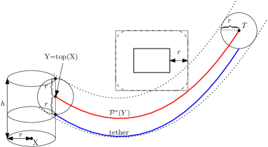
Figure 1: Model of the marsupial system with the UGV and the UAV positioned at $X$ and $T$, respectively. The UAV path with minimum length between $Y=top(X)$ and $T$ is denoted as $\mathcal{P}^{*}(Y)$ and has the same shape as the tether. An enlarged obstacle is also depicted.

In this work, we model obstacles as orthogonal cuboids  This is not a strong limitation from a practical point of view, as typical objects (e.g., walls, beams, or boxes) can be modeled as cuboids, and more complex structures can also be constructed by combining orthogonal cuboids.

For handling collisions involving both the UAV and the tether, we consider the following definition. We refer the UAV’s path to the path followed by the center of the sphere, and we say that the UAV’s path is collision-free if the locus of points equidistant from the path at distance $r$ does not cross any obstacle. With this definition, a tether below the UAV’s path at vertical distance $r$ does not intersect any obstacle. See Figure 1. We assume that the UAV has a path tracker that allows it to fly paths with the same shape as the tether.

The following transformation is useful for collision checking. We expand each obstacle by performing the Minkowski sum with the sphere of radius $r$ and consider the minimum cuboid that contains the expanded obstacle. Then, we shrink the UAV sphere down to its central point and we say that the UAV’s path is collision-free when it does not cross any of the enlarged cuboids. With this transformation, the geometry of the obstacles is preserved, avoiding curved boundaries that complicate computation and are impractical in real applications. Since we consider a taut tether, we assume that no collision occurs if the path is tangent to an obstacle. Additionally, with this transformation, the cylinder representing the marsupial robotics system (while carrying the UAV) shrinks down to a vertical segment of length $h-r$ and we say that the UGV’s path is collision-free if this vertical segment does not cross any of the enlarged obstacles.

III Optimization Problem and Strategy Overview

Given the marsupial robotics system described in Section II, we address an optimization path planning problem where the goal is to minimize the time to reach a given aerial target point. We assume a strategy in which the UGV first navigates (with the UAV) to a point on the ground from which the UAV can take off and reach the target. We consider a constant traveling speed for both vehicles, so the objective function to optimize is the sum of the distances traveled by the vehicles, that is, the sum of the lengths of the UGV path and the UAV path. We formally define the optimization problem as follows:

Shortest Marsupial Path Problem (SMPP): Let $h$, $r$ and $L$ be positive numbers. Given a 3D scenario with a set $\mathcal{O}$ of $n$ orthogonal cuboids, a point $S$ in the plane $z=0$ (the ground), and a target point $T$ in the aerial region $z>h$, we want to find a point $X$ on the ground such that:

1. There exists a path $P_{g}$ from $S$ to $X$ so that the marsupial robot (modeled as a vertical segment of height $h-r$) can traverse $P_{g}$ without colliding with obstacles in $\mathcal{O}$.

2. Given the vertical plane $\pi_{X,T}$ passing through $X$ and $T$, there exists a collision-free path $P_{a}$ from $top(X)$ to $T$ within $\pi_{X,T}$ for the UAV (modeled as a point).

3. There exists a controllable, loose tether of length at most $L$ that can follow the UAV along the path $P_{a}$.

4. The sum of the lengths of $P_{g}$ and $P_{a}$ is minimized.

The tether can be modeled either with a catenary curve (loose tether) or with a polygonal chain (taut tether). Firstly, we approximate the solution of the SMPP using a taut tether modeled with an increasing convex polygonal chain (to be defined later) that, in general, is supported by the obstacles. Subsequently, we demonstrate that this approach can significantly enhance computational efficiency in problems involving catenaries.

In the following, we assume a 3D scenario with a set $\mathcal{O}$ of $n$ orthogonal cuboids and a marsupial system model as defined above.

Definition 1.

Given $L>0$, we say that the point $top(X)$ is $L$-polygonal-visible ($p_{L}$-visible for short) if there exists a collision-free, taut tether, modeled as a polygonal chain, connecting $top(X)$ and $T$ with a length of at most $L$.

We introduce the following two subproblems that contribute to the solution of the SMPP:

Polygonal Visibility Problem (PVP): Given two positive numbers $h$ and $r$, with $h>2r$, compute the locus of $p_{L}$-visible points within the horizontal plane $\pi_{top}\equiv z=h-r$.

Minimum Length Tether Problem (MLTP): Given $top(X)$ and $T$, compute the shortest length of a collision-free taut tether, if there is one, connecting $top(X)$ and $T$, and contained in the vertical plane $\pi_{X,T}$.

Assuming a taut tether, the strategy proposed in this work to solve SMPP (MASPA: Marsupial Sequential Path-Planning Approach) is based on the following: we first compute a discrete set of $p_{L}$-visible candidate take-off points in the space, each one with an associated UGV candidate position on the ground. Then, we create a visibility graph generated by the initial point $S$, the ground obstacles, and the candidate positions on the ground. Finally, we use this graph to plan a collision-free path for the UGV from $S$ to the best candidate point from which the UAV can take off and reach $T$, so that the sum of the aerial and ground paths is minimized. In addition, we extend these ideas to apply to scenarios that involve a loose tether instead of a taut one. Figure 2 shows a scenario of the marsupial path planning problem and two possible solutions.

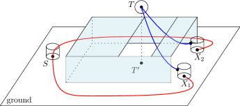
Figure 2: An scenario of the marsupial path planning problem. Two paths are required, a ground path (red) for the UGV carrying the UAV from the starting point $S$ to a ground point $X$ from which the UAV can reach the target $T$ using a collision-free aerial path (blue). In the scenario, two possible solutions are showed; the general problem is to find the one that minimizes the sum of the lengths.

IV Polygonal Visibility Problem

In this section, we propose a competitive algorithm to tackle PVP. First, we define a 2D version of the problem (PVP-2D) looking for the locus of $p_{L}$-visible points within a vertical plane that contains $T$ (Section IV-A). Then, we describe some geometrical properties (Section IV-B) and introduce a novel algorithm (PVA-2D) to solve PVP-2D (Section IV-C). This algorithm is the core of our work, as it significantly reduces the computation time of the overall path planner MASPA. In Section IV-D, we prove the correctness and time complexity of PVA-2D; and in Section IV-E, we discuss extensions of the algorithm. Finally, based on PVA-2D, we propose an algorithm (PVA-3D) to solve PVP in 3D scenarios (Section IV-F).

IV-A PVP-2D Statement

After taking off, the motion of the UAV is constrained to the vertical plane $\pi_{X,T}$, hence we address PVP in two dimensions. The intersection of the marsupial system (represented as a cylinder in 3D) with $\pi_{X,T}$ results in a rectangle; and, after the obstacles are enlarged, it becomes a segment of height $h-r$ perpendicular to the ground at position $X$. In addition, the 3D obstacles modeled as cuboids become rectangles. Figure 3 shows a representation of the 2D problem.

We first introduce some definitions, followed by the problem statement. Let $v_{0},v_{1},\cdots,v_{k}$ be the vertices, ordered from left to right, of a polygonal chain $\mathcal{P}$ in the plane. A polygonal chain is defined by its vertices; i.e., $\mathcal{P}=\{v_{0},v_{1},\cdots,v_{k}\}$.

• We say that a vertex $v_{i}$ is a convex vertex, $i\neq\{0,k\}$, if $v_{i}$ is to the right of (or lies on) the directed line from $v_{i-1}$ to $v_{i+1}$; when all $v_{i}$ are convex we say that $\mathcal{P}$ is a convex polygonal chain.

• Given a point $p$, we denote by $NE(p)$ the region of the plane to the right and above $p$. When $v_{i}\in NE(v_{i-1}),\,i=1,\dots,k,$ we say that $\mathcal{P}$ is an increasing polygonal chain.

• A polygonal chain that does not cross any obstacle in the plane is collision-free.

We denote a Collision-free Increasing Convex Polygonal chain (CICP for short) from point $Y=top(X)$ to target $T$ by $\mathcal{P}(Y)$, and $\mathcal{P}^{*}(Y)$ will be the $\mathcal{P}(Y)$ of minimum length.

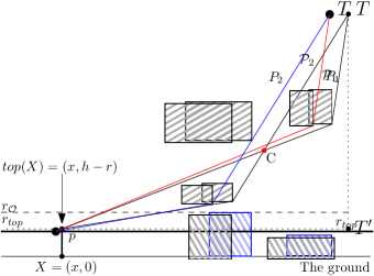
Figure 3: An intance of PVP-2D. Aerial obstacles are in gray and ground obstacles in blue. The chains $\mathcal{P}_{1}$ and $\mathcal{P}_{2}$ are two CICPs from $top(X)$ to $T$. The point $C$ represents the crossing point where $\mathcal{P}_{1}$ crosses $\mathcal{P}_{2}$.

We propose the following two-dimensional problem:

PVP-2D: Consider three parallel lines in a vertical plane: $y=0$, the ground; $\text{$r_{top}$}{}\equiv y=h-r$, the take-off line; and $r_{\mathcal{O}}\equiv y=h$; and the point $T$ above them. Let $\mathcal{O}$ be the set of $n$ obstacles modeled as isothetic rectangles above the ground. We want to compute all points $Y=top(X)$ in $r_{top}$, with $X=(x,0)$ on the ground to the left of $T$, fulfilling the following conditions:

1. the marsupial system within the vertical plane located at $X$, i.e., the vertical segment with height $h-r$ and lowest endpoint $X$, does not intersect any obstacle in $\mathcal{O}$;

2. the point $Y$ is $p_{L}$-visible, which means that there exists a path $\mathcal{P}(Y)$ with at most length $L$ from $Y$ to $T$.

In order to solve PVP-2D, we divide the set of obstacles $\mathcal{O}$ into two subsets: $\mathcal{O}_{a}$ and $\mathcal{O}_{g}$, representing aerial and ground obstacles, respectively. For simplicity, from now on we assume that: 1) the obstacles in $\mathcal{O}_{g}$ are below the line $r_{\mathcal{O}}$, while the base of the obstacles in $\mathcal{O}_{a}$ is placed above the line $r_{\mathcal{O}}$ (see Figure 3); 2) the obstacles are completely contained in the semiplane to the left of the segment $\overline{TT^{\prime}}$, where $T^{\prime}$ is the orthogonal projection of $T$ onto $r_{top}$.

Let $[(a_{i},0),(b_{i},0)]$ be the interval of points on the ground covered by the $i$-th ground obstacle. It is easy to see that all points $X=(x,0)$, such that $x\notin[a_{i},b_{i}]$ for every $i\in[1,2,\ldots,|\mathcal{O}_{g}|]$, meet Condition I. From Condition II, we need to find the intervals of non $p_{L}$-visible take-off points in $r_{top}$ to the left of $T$, giving us the following definition.

Definition 2.

Let $(A,B)$ be an open interval in $r_{top}$, such that $A$ and $B$ are $p_{L}$-visible points. If each point within $(A,B)$ is non $p_{L}$-visible, then we call $(A,B)$ a maximal non $p_{L}$-visible interval, where $A$ and $B$ are named the left and right end-points, respectively.

In the following, we give some properties and propose an algorithm to solve PVP-2D calculating the set of maximal non $p_{L}$-visible intervals contained in $[Q,T^{\prime}]$, where $Q$ is the point in $r_{top}$ at distance $L$ from $T$ to the left of $T^{\prime}$ .

IV-B PVP-2D Properties

For the $i$-th isothetic rectangle in $\mathcal{O}_{a}$, we denote $u_{i}$ (resp. $l_{i}$) its upper-left (resp. lower-right) vertex (see Figure 4). We refer to these points as critical vertices. The following properties are useful for designing the PVP-2D algorithm and are straightforward to prove:

Lemma 1.

Given $A,B\in\text{$r_{top}$}{}$ and $(A,B)$ a maximal non $p_{L}$-visible interval, then there exists $\mathcal{P}^{*}(A)$, with $|\mathcal{P}^{*}(A)|=k>2$, such that: 1) for all $j\notin\{0,1,k-1\}$ the vertices $v_{j}$ of $\mathcal{P}^{*}(A)$ are the lower-right vertices of some aerial obstacles; 2) $v_{1}$ is the upper left vertex of an aerial obstacle; 3) $v_{0}$, $v_{1}$, and $v_{2}$ are colinear; and 4) $A$ is the rightmost point so that $\mathcal{P}^{*}(A)$ contains $v_{1}$.

Lemma 2.

Given $A,B\in\text{$r_{top}$}{}$ and $(A,B)$ a maximal non $p_{L}$-visible interval, then there exists $\mathcal{P}^{*}(B)$, such that for each $j\notin\{0,k-1\}$, with $|\mathcal{P}^{*}(B)|=k>1$, the vertices $v_{j}$ of $\mathcal{P}^{*}(B)$ are the lower-right vertices of some aerial obstacles. In addition, the length of $\mathcal{P}^{*}(B)$ is $L$.

Figure 4: The red and blue points in $r_{top}$ indicate the vertices of the minimum opening and closing CICPs, respectively. Notice that the red point $l_{2}$ belongs to the red $\mathcal{P}^{*}(B_{2})$ and to the blue $\mathcal{P}^{*}(A_{4})$ simultaneously. Furthermore, notice that although $\mathcal{P}^{*}(B_{2})$ and $\mathcal{P}^{*}(A_{4})$ coincide between $l_{2}$ and $T$, $l_{2}$ is not a crossing point. The take-off point $Q$ is the leftmost point that can reach $T$ with a tether of maximum length $L$.

Figure 4 shows the non $p_{L}$-visible intervals $(A_{2},B_{2})$ and $(A_{4},B_{5})$ for a scenario with five isothetic rectangular obstacles to the left of $T$. The critical vertices $l_{i}$ and $u_{i}$ ($i=1,\cdots,5$) are shown.

Definition 3.

Let $C\neq T$ be the rightmost common point of two given CICPs $\mathcal{P}_{1}$ and $\mathcal{P}_{2}$; and let $v_{1}$ and $v_{2}$ be the first vertices to the right of $C$ in $\mathcal{P}_{1}$ and $\mathcal{P}_{2}$, respectively. We call $C$ a crossing-point when the segments $\overline{Cv_{1}}$ and $\overline{Cv_{2}}$ have different slopes. If the slope of $\overline{Cv_{1}}$ is lower than the slope of $\overline{Cv_{2}}$, we say that $\mathcal{P}_{1}$ crosses $\mathcal{P}_{2}$, see Figure 3.

For each take-off point in the $\pi_{top}$ plane, the following lemmas are satisfied.

Lemma 3.

Let $Y,Y^{\prime}$ be two $p_{L}$-visible points in $r_{top}$, then the chain $\mathcal{P}^{*}(Y)$ does not cross any of the possible $\mathcal{P}(Y^{\prime})$ chains.

Proof.

Assume that $C$ is a point where $\mathcal{P}^{*}(Y)$ crosses $\mathcal{P}(Y^{\prime})$. Let $C^{\prime}$ be the first common point of $\mathcal{P}^{*}(Y)$ and $\mathcal{P}(Y^{\prime})$ to the right of $C$. The existence of $C^{\prime}$ is guaranteed since both chains share $T$ as a common point to the right of $C$; see an example in Figure 3. Notice that the convexity of the chains claims that the length of $\mathcal{P}(Y^{\prime})$ between $C$ and $C^{\prime}$ is shorter than the length of $\mathcal{P}^{*}(Y)$ in the same interval. Let $\mathcal{P}_{1}\subset\mathcal{P}^{*}(Y)$ be a chain from $Y$ to $C$, let $\mathcal{P}_{2}\subset\mathcal{P}(Y^{\prime})$ be a chain from $C$ to $C^{\prime}$, and let $\mathcal{P}_{3}\subset\mathcal{P}^{*}(Y)$ be a chain from $C^{\prime}$ to $T$. Notice that the chain $\mathcal{P}_{1}\cup\mathcal{P}_{2}\cup\mathcal{P}_{3}$ from $Y$ to $T$ is a CICP and its length is shorter than the length of $\mathcal{P}^{*}(Y)$. This contradiction implies that the crossing point $C$ cannot exist. ∎

Lemma 4.

Let $Y$ be a $p_{L}$-visible point in $r_{top}$. If $\mathcal{P}(Y)$ does not cross $\mathcal{P}^{*}(Y)$, then $\mathcal{P}(Y)$ and $\mathcal{P}^{*}(Y)$ coincide.

Proof.

Notice that, if $\mathcal{P}(Y)$ and $\mathcal{P}^{*}(Y)$ have only $Y$ and $T$ in common, $Y$ would be a crossing point between them. According to Lemma 3, $\mathcal{P}^{*}(Y)$ does not cross $\mathcal{P}(Y)$; therefore, if $\mathcal{P}(Y)$ does not cross $\mathcal{P}^{*}(Y)$, then both chains must coincide. ∎

IV-C Polygonal Visibility Algorithm 2D (PVA-2D)

In this section, we describe the algorithm to solve the 2D version of PVP. The algorithm computes a list of non $p_{L}$-visible intervals of take-off points in the horizontal line $r_{top}$ within a vertical plane, that is, the complementary set to the one we are looking for (Figure 4 illustrates an example). For a given point $Y$ in the vertical plane, we denote as $\mathcal{P}_{alg}(Y)$ to the $\mathcal{P}(Y)$ chain computed by the algorithm, which we denote as PVA-2D. The algorithm PVA-2D performs the following steps:

STEP 1: Compute $\mathcal{P}_{alg}(l_{j})$ recursively for all lower-right vertices $l_{j}$.

Let $l_{1},l_{2},\cdots,l_{n}$ be the lower-right vertices of the aerial obstacles arranged in decreasing order of their $y$-coordinates; and let $l_{0}$ be $T$. For each $j\in\{0,1,\cdots,n\}$, we compute, if it exists, a CICP called $\mathcal{P}_{alg}(l_{j})$ using the following two arrays:

(1) Array $\mathcal{L}$ of chain lengths, where $\mathcal{L}[j]$ stores the length of $\mathcal{P}_{alg}(l_{j})$. Initially, $\mathcal{L}[j]=\infty$ for $j\neq 0$, $\mathcal{L}[0]=0$, and the following updating rule is applied:

$$\mathcal{L}[j]=\min_{i\in I_{j}}\left\{\mathcal{L}[i]+||l_{i}-l_{j}||_{2}\right\},$$ (1)

where $i\in I_{j}$ iff $\overline{l_{j}l_{i}}\cup\mathcal{P}_{alg}(l_{i})$ is a CICP.

(2) Array of hooks $\mathcal{D}$, where $\mathcal{D}[j]$ stores $l_{i}$ with $i\in\{0,\cdots,j-1\}$, whenever $\mathcal{P}_{alg}(l_{j})=\langle l_{j},l_{i},...,T\rangle$. Initially, $\mathcal{D}[j]=\emptyset$ for all $j$. In Figure 4, $\mathcal{P}_{alg}(l_{5})=\langle l_{5},l_{4},l_{1},T\rangle$.

Notice that updating the value of $\mathcal{L}[j]$ triggers an update in the value of $\mathcal{D}[j]$, so $\mathcal{L}$ and $\mathcal{D}$ are filled simultaneously. The array $\mathcal{D}$ is used to compute $\mathcal{P}_{alg}(l_{j})$ during the process.

STEP 2: Compute the left end-points candidates of maximal non $p_{L}$-visible intervals.

For each upper-left vertex $u_{i}$, $i\in\{1,\cdots,n\}$, let $l^{*}_{j}$, for $j\in\{0,1,\cdots,n\}$, be the lower-right vertex such that $\overline{u_{i}l^{*}_{j}}\cup\mathcal{P}_{alg}(l^{*}_{j})$ is a CICP and $\overline{u_{i}l^{*}_{j}}$ has maximum slope (Lemma 6 justifies this selection). Let $A^{*}_{i,j}$ be the intersection point between $r_{top}$ and the line passing through $u_{i}$ and $l^{*}_{j}$. We create the following two arrays:

(3) Array $\mathcal{A}$ of the left end-points candidates:

$$\mathcal{A}[i]=\begin{cases}A^{*}_{i,j},&\text{ if }\|A^{*}_{i,j}-l^{*}_{j}\|_{2}+\mathcal{L}[j]\leq L\text{ and,}\\ &\overline{A^{*}_{i,j}l^{*}_{j}}\cap\mathcal{O}_{a}=\emptyset\\ \emptyset,&\text{ otherwise. }\\ \end{cases}$$ (2)

(4) Array of hooks $\mathcal{U}$, where $\mathcal{U}[i]$ stores the point $l^{*}_{j}$ if $\mathcal{A}[i]=A^{*}_{i,j}$. Initially, $\mathcal{U}[i]=\emptyset$ for all $i$.

For the sake of simplicity, as there can only be one $A^{*}_{i,j}$ for each $u_{i}$, we denote $A^{*}_{i,j}$ as $A_{i}$. See the left end-point $A_{4}$ in Figure 4. The arrays $\mathcal{L}$ and $\mathcal{D}$ are used to compute the array $\mathcal{A}$.

STEP 3: Compute the right end-points of maximal non $p_{L}$-visible intervals.

For each $j$, with $\mathcal{L}[j]<\infty$, take the point $B_{j}\in\text{$r_{top}$}$ to the left of $l_{j}$ such that $\|B_{j}-l_{j}\|_{2}=L-\mathcal{L}[j]$, if it exists. We create the following array:

(5) Array $\mathcal{B}$ of right end-points. Initially, $\mathcal{B}[j]=\emptyset$ for all $j$. Then, we apply the update rule $\mathcal{B}[j]=B_{j}$ if:

1. $\overline{B_{j}l_{j}}\cup\mathcal{P}_{alg}(l_{j})$ is a CICP.

2. There is no $l_{k}$ so that $\overline{B_{j}l_{k}}\cup\mathcal{P}_{alg}(l_{k})$ is a CICP with length lower than $L$. Notice that, by definition of $B_{j}$, the length of $\overline{B_{j}l_{j}}\cup\mathcal{P}_{alg}(l_{j})$ is exactly $L$. To illustrate this property, imagine that in Figure 4, the obstacle labeled as 4 were not present; then the vertex $l_{2}$ could be used to invalidate $B_{5}$.

STEP 4: Compute the $p_{L}$-visible intervals.

We create the list $\mathcal{H}$ that contains all $A_{i}$ and $B_{j}$ found in the previous steps and sort it from left to right. We consider the interval $(A_{i},B_{j})$ as non $p_{L}$-visible when $B_{j}$ immediately succeeds $A_{i}$ (from left to right) in $\mathcal{H}$. If two left end-points $A_{i}$ and $A_{k}$ are consecutive (from left to right), then $A_{i}$ is rejected.

We create the set $\mathcal{I}$ with the non $p_{L}$-visible intervals obtained from $\mathcal{H}$. In the case where $\mathcal{H}$ starts with a right end-point candidate $B_{j}$, we add to $\mathcal{I}$ the interval $[Q,B_{j})$. Finally, the output of PVA-2D, which is the set of $p_{L}$-visible intervals, is the complement of $\mathcal{I}$ within the interval $[Q,T^{\prime}]$ in $r_{top}$.

IV-D PVP-2D Algorithmic Correctness and Complexity

In this section, we prove the correctness of PVA-2D based on the geometrical properties of the problem. Then, we study its computational cost.

Remark 1.

All take-off points $Y\in\mathcal{H}$ (STEP 4 of PVA-2D) are $p_{L}$-visible.

Remark 2.

For each $l_{j}$, $\mathcal{P}_{alg}(l_{j})=\mathcal{P}^{*}(l_{j})$ (see Equation (1)). Therefore, the array $\mathcal{L}$ stores in position $j$ the length of $\mathcal{P}^{*}(l_{j})$.

From these Remarks, we can prove the following results:

Lemma 5.

Let $Y\neq Q$ be a point in $r_{top}$. The length of $\mathcal{P}^{*}(Y)$ is $L$ if and only if $Y\in\mathcal{B}$ (STEP 3 of PVA-2D).

Proof.

Let $Y$ be a point in $r_{top}$, and $\mathcal{P}^{*}(Y)$ be a CICP in which all vertices except for $Y$ and $T$ are lower-right vertices of aerial obstacles; this chain exists according to Lemma 2. We use $\mathcal{P}^{*}(Y)$ in both directions of the proof.

Consider $\mathcal{P}^{*}(Y)$ of length $L$. If $l_{j}$ is the second vertex of $\mathcal{P}^{*}(Y)$, then, using Remark 2 there exists $\mathcal{P}^{*}(l_{j})$ such that:

$$\mathcal{P}^{*}(Y)=\overline{Yl_{j}}\cup\mathcal{P}^{*}(l_{j})=\overline{Yl_{j}}\cup\mathcal{P}_{alg}(l_{j})$$

This implies that $|\overline{Yl_{j}}|+\mathcal{L}[j]=L$, and consequently, that $Y$ is considered a candidate for right end-point of a non $p_{L}$-visible interval in STEP 3 of PVA-2D. As there is no CICP shorter than $\mathcal{P}^{*}(Y)$ connecting $Y$ and $T$, $Y$ is stored in $\mathcal{B}[j]$.

Now, let $Y=\mathcal{B}[j]$ be selected in STEP 3 of PVA-2D. Assume that $\mathcal{P}_{alg}(Y)$ does not coincide with $\mathcal{P}^{*}(Y)$. As a corollary of Lemma 4, $\mathcal{P}_{alg}(Y)$ would cross $\mathcal{P}^{*}(Y)$ and the length of $\mathcal{P}^{*}(Y)$ would be strictly lower. Let $l_{k}$ be the second vertex of $\mathcal{P}^{*}(Y)$. According to Remark 2, there exists $\mathcal{P}^{*}(l_{k})$ such that:

$$\mathcal{P}^{*}(Y)=\overline{Yl_{k}}\cup\mathcal{P}^{*}(l_{k})=\overline{Yl_{k}}\cup\mathcal{P}_{alg}(l_{k})$$

As the length of $\mathcal{P}_{alg}(Y)$ is $L$ (STEP 3), it holds that $|\overline{Yl_{k}}|+\mathcal{L}[k]<L$. Consequently, the point $Y$ would be discarded as the right end-point of a maximal non $p_{L}$-visible interval in STEP 3 (b). This argument contradicts the assumption that $Y=\mathcal{B}[j]$; therefore, $\mathcal{P}_{alg}(Y)$ and $\mathcal{P}^{*}(Y)$ must coincide, and the result follows. ∎

Lemma 6.

If $(A,B)$ is a maximal non $p_{L}$-visible interval found in list $\mathcal{H}$ at STEP 4 of PVA-2D, then $A$ is the first $p_{L}$-visible point to the left of $B$ in $r_{top}$.

Proof.

According to Lemma 5, $\mathcal{P}^{*}(B)$ and $\mathcal{P}_{alg}(B)$ coincide and both have length $L$. Let $Y$ be the first $p_{L}$-visible point in $r_{top}$ to the left of $B$. As the length of $\mathcal{P}^{*}(B)$ is $L$, if $Y$ exists, then $(Y,B)$ is a maximal non $p_{L}$-visible interval.

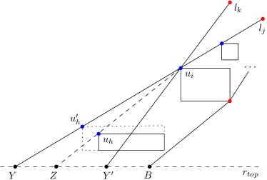
Figure 5: Proof of Lemma 6. Segment $\overline{u_{i}l_{j}}$ is the one with greatest slope if $Y$ is the first $p_{L}$-visible point to the left of $B$.

Now, let $u_{i}$ and $l_{j}$ the second and third vertices of the CICP $\mathcal{P}^{*}(Y)$ as stated in Lemma 1. Without loss of generality, we assume that $u_{i}$ is the lowest upper-left vertex if there are several. Refer to Figure 5. We can prove that, if $Y$ is the first $p_{L}$-visible to the left of $B$, then the segment $\overline{u_{i}l_{j}}$ has the highest slope among all pairs $(u_{i},l_{k})$ so that $\overline{u_{i}l_{k}}\cup\mathcal{P}_{alg}(l_{k})$ is a CICP. Suppose, on the contrary, that there exists a segment $\overline{u_{i}l_{k}}$ where $\overline{u_{i}l_{k}}\cup\mathcal{P}_{alg}(l_{k})$ is a CICP and $\overline{u_{i}l_{k}}$ has a greater slope than $\overline{u_{i}l_{j}}$, as shown in Figure 5; and let $Y^{\prime}$ be the intersection point between $r_{top}$ and the line containing $\overline{u_{i}l_{k}}$. As there is no $p_{L}$-visible point in $r_{top}$ between $Y$ and $B$, there exits an obstacle below $O_{i}$ that intersects the segment $Y^{\prime}u_{i}$. Moreover, there exists an obstacle that necessarily touches the segment $\overline{Yu_{i}}$. In this case, $u_{i}$ is not lowest left-upper vertex of $\mathcal{P}^{*}(Y)$, leading to a contradiction. As PVA-2D selects the pair $\overline{u_{i}l_{j}}$ with the greatest slope, $Y=A$ and the Lemma follows. ∎

Theorem 1.

Let $Y$ be a point in the interval $[Q,T^{\prime}]$ in $r_{top}$. The point $Y$ is non $p_{L}$-visible if and only if $Y$ belongs to an interval in the set $\mathcal{I}$ found in STEP 4 of PVA-2D.

Proof.

Let $Y$ be a point in $r_{top}$. If $Y$ belongs to an interval $(A,B)$ of $\mathcal{I}$, then according to Lemma 6, $A$ is the first $p_{L}$-visible point to the left of $B$ in $r_{top}$. If $Y$ belongs to the interval $[Q,B)$ of $\mathcal{I}$, then as a corollary of Lemma 6, there are no $p_{L}$-visible points to the left of $B$ in $r_{top}$. In either case, $Y$ is a non $p_{L}$-visible point.

For the reverse implication: let $Y$ be a non $p_{L}$-visible point. Let $B$ be the first $p_{L}$-visible point in $r_{top}$ to the right of $Y$. Notice that $\mathcal{P}^{*}(B)$ must have length $L$; therefore, according to Lemma 5, PVA-2D finds $B$ as the right end-point of a maximal non $p_{L}$-visible interval in STEP 3. Now, let $A$ be the first $p_{L}$-visible point in $r_{top}$ to the left of $Y$. If $A$ exists, then according to Lemma 6, the algorithm selects $(A,B)$ as a maximal non $p_{L}$-visible in STEP 4. If $A$ does not exist, then $B$ would be the first point in the list $\mathcal{H}$, and the interval $[Q,B)$ would be added to $\mathcal{I}$ in STEP 4. In either case, $Y$ belongs to an interval in $\mathcal{I}$, and the result follows. ∎

Now, we establish the computational complexity of PVA-2D, assuming that a visibility graph is used. Notice that computing the visibility graph of a collection of disjoint polygons in the plane with a total of $n$ edges takes $O(n^{2})$ time [5].

Theorem 2.

PVA-2D takes $O(n^{2})$ time to compute the set of $p_{L}$-visible intervals.

Proof.

As a pre-processing step, we build a visibility graph between $T$ and the aerial obstacles. The visibility graph allows us to check in $O(1)$ time whether all two critical vertices are visible. As we consider $n$ rectangular obstacles and the point $T$, the total number of vertices in the graph will be $4n+1$, and this process takes $O(n^{2})$ time.

(STEP 1) We sort the lower-right critical vertices $l_{i}$ in decreasing order of height in $O(n\log n)$ time. Then, the arrays $\mathcal{L}$ and $\mathcal{D}$ of PVA-2D can be calculated with two nested loops on the sorted $l_{i}$ vertices, taking $O(n^{2})$ time.

(STEP 2) The candidates for left end-point of maximal non $p_{L}$-visible interval can be calculated in $O(n^{2})$ time as follows. For each $u_{i}$, we compute in $O(n)$ time the associated left end-point as follows. First, compute the $l_{j}$ vertex so that $\{u_{i}\}\cup\mathcal{P}_{alg}(l_{j})$ is a CICP and $\overline{u_{i}l_{j}}$ has the maximum slope. Let $A_{i}$ be the associated point in $r_{top}$ such that $u_{i}\in\overline{A_{i}l_{j}}$. Second, if $\overline{A_{i}l_{j}}$ does not collide with any obstacle, then $A_{i}$ is a candidate to left end-point of interval and we set $\mathcal{U}[i]=A_{i}$; else, according to Lemma 6, we do not need to check for more pairs $(u_{i},l_{k})$ and we avoid quadratic time at this step. Therefore, as we require only $O(n)$ time for each $u_{i}$, the total time to fill the array $\mathcal{A}$ is $O(n^{2})$ time.

(STEP 3) Afterward, to fill the array $\mathcal{B}$, we must search for all points $B_{j}$ in $r_{top}$ such that $\{B_{j}\}\cup\mathcal{P}_{alg}(l_{j})$ forms a CICP of length $L$. For each $l_{j}$, we calculate the point $B_{j}$ in $O(1)$ time. We then add all candidates $B_{j}$ to the precomputed visibility graph, taking $O(n^{2})$ in the worst case. The updated visibility graph enables us to check whether there exists a lower-right vertex $l_{k}$ such that $\{B_{j}\}\cup\mathcal{P}_{alg}(l_{k})$ forms a CICP of length lower than $L$. If such a $l_{k}$ exists, then $B_{j}$ is discarded as a candidate. Since there are at most $n$ candidates $B_{j}$, the $\mathcal{B}$ array can be filled in $O(n^{2})$ time.

(STEP 4) Finally, the list $\mathcal{H}$ is created in $O(n)$ time by joining the points $A_{i}$ and $B_{j}$. We sort this list in $O(n\log n)$ time and the maximal non $p_{L}$-visible intervals in the $\mathcal{I}$ array can be computed with a left-to-right sweep over $\mathcal{H}$ in $O(n)$ time. The output of the algorithm is the complement of $\mathcal{I}$ in the interval $[Q,T^{\prime}]\in\text{$r_{top}$}$. ∎

Notice that, since the number of vertices per obstacle is constant, the complexity of the algorithm depends entirely on the number of obstacles. Another observation is that if we are given the sorted list of $p_{L}$-visible intervals, determining whether a query point $Y$ in $r_{top}$ is $p_{L}$-visible can be answered in $O(\log{n})$ time using binary search.

IV-E Extensions

This section discusses how our algorithm could be extended by relaxing some of the initial assumptions:

• Ground obstacles above the $r_{\mathcal{O}}$ line. Let $O$ be an obstacle on the ground with height greater than $h$. As with the rest of the ground obstacles, we first use $O$ to discard the intervals of points on the ground where the UGV would collide. After that, $O$ should be considered as another aerial obstacle for the rest of the algorithm; but notice that there is no need to consider its lower-right vertex as part of any CICP in the PVA-2D, as that vertex is on the ground.

• Aerial obstacles below $r_{\mathcal{O}}$.

  Let $O$ be an aerial obstacle below $r_{\mathcal{O}}$. In this case, $O$ can also be considered as a ground obstacle, since the marsupial system cannot pass below it. Thus, we have to use this obstacle in the preprocessing step to discard the intervals where the UGV cannot enter. Besides, this obstacle should also be considered as another aerial obstacle in the rest of the algorithm. Notice that a special case could occur: a polygonal line from a point $Y\in\text{$r_{top}$}{}$ to $T$ could be tangent to the base of $O$ and touch both its lower (left and right) vertices that support the bottom face. Consequently, the array $\mathcal{L}$ used in PVA-2D to store the length of $\mathcal{P}^{*}$ from each lower-right vertex to $T$, can also be used to store the length of $\mathcal{P}^{*}$ from each lower-left vertex to $T$ without altering the time complexity of $O(n^{2})$ of STEP 2. Furthermore, since now there could be polygonal lines below $r_{\mathcal{O}}$, ground obstacles must also be considered in tether collision check.

• Obstacles on both sides of $T$. Let us call central obstacles those intersecting the segment $\overline{TT^{\prime}}$, where $T^{\prime}$ is the orthogonal projection of $T$ on the ground. The problem can be solved independently in each halfplane defined by $\overline{TT^{\prime}}$. The only two updates we need to make to include these obstacles to PVA-2D are: (1) do not calculate the CICP $\mathcal{P}_{alg}(l_{c})$ in STEP 1 for all lower-right vertices of central obstacles $l_{c}$ and, (2) consider the projection point $T^{\prime}$ as the right-endpoint of a maximal non $p_{L}$-visible interval in STEP 4.

• Different types of obstacles. The algorithm can be easily extended to non-rectangular obstacles. In that case, CICPs of minimum length could be tangent to many sides of the obstacles. Basically, we have a convex chain that plays the role of the vertex $u_{i}$. Therefore, in the array $\mathcal{L}$, we would have to store the length of $\mathcal{P}^{*}(v)$, for each vertex $v$ of each obstacle.

The complexity of PVA-2D depends entirely on the total number of vertices. It is easy to see that the above extensions can be solved in the same $O(n^{2})$ time, with $n$ being the total number of vertices of the obstacles.

IV-F Polygonal Visibility Algorithm 3D (PVA-3D)

In this section, we show how to use the PVA-2D algorithm to design an approximation algorithm, PVA-3D, for the general polygonal visibility problem in 3D, where the goal is to compute the locus of all $p_{L}$-visible points in the plane $\pi_{top}$. The idea is to consider a beam of $p$ planes, passing through $T$ and perpendicular to the ground, and use PVA-2D in each plane. Obviously, the more planes considered, the better approximation of the $p_{L}$-visible region we have.

Consider the circle on $\pi_{top}$ centered at $T^{\prime}$ with radius $r=\sqrt{L^{2}-|\overline{TT^{\prime}}|^{2}}$, which contains all feasible take-off points. We uniformly divide the space into a set $\mathcal{\pi}=\{\pi_{1},\pi_{2},\dots,\pi_{p}\}$ of $p$ vertical planes containing $T$ and the output of applying PVA-2D in these planes gives an approximation to the 2D region of $p_{L}$-visible points. See Figure 6.

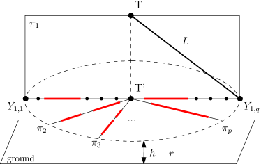
Figure 6: Approximated solution for PVP-3D. For each plane $\pi_{i}$, a discrete set $\mathcal{Y}_{i}$ is considered as feasible take-off points. The red segments indicate non $p_{L}$-visible intervals in each vertical plane.

V MArsupial Sequential Path-planning Approach (MASPA)

In this section, we are ready to describe our strategy to solve the problem SMPP for a tethered marsupial system. This strategy, MASPA, navigates the UGV from a starting position $S$ to a specified point denoted $X$. Subsequently, the UAV can be deployed from this location to successfully reach the aerial target $T$.

Assume that a solution of PVA-3D is given as in Section IV-F. In each plane, we consider a discrete set $\mathcal{Y}_{i}=\{Y_{i,1},\dots,Y_{i,q}\}$ of $q$ take-off candidate points uniformly distributed along the $p_{L}$-visible intervals, where $Y_{i,j}$ is the $j^{th}$ candidate in the $i^{th}$ vertical plane. See Figure 6 for an illustration of the process. Let $\mathcal{P}^{*}(Y_{i,j})$ be the minimum length CICP path for the UAV between $Y_{i,j}$ and $T$. Recall that, for each plane $\pi_{i}$, PVA-2D stores in the array $\mathcal{L}$ the length of $\mathcal{P}_{alg}(l_{k})$, for each lower-right vertex $l_{k}$. With this information, we can compute $\mathcal{P}^{*}(Y_{i,j})$ for the point $Y_{i,j}$ in $O(n^{2})$ time by checking each possible segment $\overline{Y_{i,j}l_{k}}$ for collisions and keeping the one that defines the shortest path. Therefore, we compute the discrete set of $p_{L}$-visible take-off points in $O(pqn^{2})$ time, where $pq$ represents the maximum number of candidate points.

Let $G=(V,E)$ be the visibility graph on the ground where the set of vertices $V$ is defined by the starting point of the UGV, $S$, the vertices of the projection on the ground of the obstacles in $\mathcal{O}_{g}$, and the set of the UGV positions $X_{i,j}$ corresponding to the $p_{L}$-visible $Y_{i,j}$ points, that is, $Y_{i,j}=top(X_{i,j})$.

An edge is included in $E$ for every pair of vertices $v_{i},v_{j}$ in $V$ if the UGV can travel from $v_{i}$ to $v_{j}$ in a straight line without collision (recall that the UGV is modeled by a vertical segment according to the model explained in Section II). As obstacles are cuboids, their projection on the ground has 4 vertices; therefore, the number of elements in the set $V$ is at most $4n+pq+1$. Note that $G$ could be partially computed in a preprocessing step when the obstacles in the space are known in advance, which would ease the overall computational effort for problem instances involving multiple target points.

The criterion in the optimization problem SMPP is to minimize the sum of the UGV and UAV paths. To address this, we add an extra vertex $T^{\prime}$ in the graph $G$ and connect $T^{\prime}$ to each candidate point $Y_{i,j}$ so that the weight of the $\langle Y_{i,j}T^{\prime}\rangle$ edge is equal to the length of $\mathcal{P}^{*}(Y_{i,j})$. In this way, any path from $S$ to $T^{\prime}$ contains the sum of the path lengths of both vehicles. With the visibility graph at hand, we can apply a graph search approach (such as, for example, the Dijkstra algorithm) to find the shortest path from $S$ to $T^{\prime}$.

The computational complexity of MASPA is related to the size of the graph $G$. As $V$ contains at most $4n+pq+2$ vertices (considering $S$ and $T^{\prime}$), Dijkstra’s algorithm spends $O((n+pq)^{2})$ time. As a result, the total time complexity of MASPA is $O(pq(n^{2}+pq))$ time, where $O(pqn^{2})$ is the cost of computing the $p_{L}$-visible take-off points. Notice that if $n$ is large enough and the parameters $q$ and $p$ are considered constants, the overall complexity of the MASPA strategy is $O(n^{2})$ time.

VI Controllable Loose Tethers

In this section, we introduce a variant of the planner MASPA to efficiently solve SMPP in scenarios involving loose tethers. In this case, we assume that the marsupial system carries a device to control the length of the tether (with a maximum length of $L$). We introduce a new concept: a take-off point $Y=top(X)$ is catenary-visible, $c_{L}$-visible for short, if there exists a collision-free loose tether between $Y$ and $T$ that is modeled by a catenary curve with length equal to or lower than $L$. Then, we redefine the PVP problem for catenary curves.

Catenary Visibility Problem (CVP): Compute the locus of the $c_{L}$-visible points in $\pi_{top}$.

Notice that, when we consider catenaries, the MLTP problem does not change its statement, although we must modify the procedure to obtain the minimum length tether by considering feasible catenary curves. To efficiently solve CVP and MLTP for loose tethers, we use the following result in 2D:

Lemma 7.

If a point $Y\in r_{top}$ is non $p_{L}$-visible, then it is also not $c_{L}$-visible.

Proof.

Let $Y$ be a $c_{L}$-visible point; then there exists a catenary of length equal to or less than $L$ connecting $Y$ and $T$. That controllable tether could be tensioned until it transforms into a polygonal line of length equal to or less than $L$, and the result follows. ∎

As we did in Section IV-F, we can generate a discrete set of $p$ vertical planes passing through $T$ and a discrete set of $q$ take-off candidate points in each plane along the $p_{L}$-visible-intervals. Notice that, according to Lemma 7, the non $p_{L}$-visible points cannot be $c_{L}$-visible either. For each of the candidate take-off points, $Y_{i,j}$, we use an additional optimization algorithm to find the collision-free catenary with minimum length from $Y_{i,j}$ to $T$.

The computation of the collision-free catenaries of minimum length from a take-off point to $T$ is out of the scope of this work; see, for instance, [17] and [4] for some related papers. However, in order to conduct experiments to test the MASPA strategy, we approximate the MLTP by selecting a discrete number of tether lengths to check, with values between $\overline{Y_{i,j}T}$ and $L$, which are the minimum and maximum possible lengths. Given two anchor points and the length, we can calculate the equation of the catenary curve, and collisions between a catenary curve and the $n$ rectangular obstacles can be checked in $O(n)$. Assuming that the computation of a single catenary can also be performed in $O(1)$ time, if we consider a number of $c$ catenary lengths to test from a point $Y_{i,j}$, then the computational time required to find the tether with minimum length connecting $Y_{i,j}$ and $T$ is $O(cn)$ time. Therefore, the total time to calculate the catenary with minimum length from a set of $q$ feasible take-off points in one vertical plane is $O(n^{2}+cqn)$, where $O(n^{2})$ is the cost of solving the PVP-2D algorithm in the plane. After doing this process for every vertical plane, the total cost is $O(pn(n+cq))$ time.

Having the length of the minimum tether for the considered take-off points, the MASPA strategy can be used as we did in the case of taut tethers, i.e., by applying Dijkstra’s algorithm over an augmented visibility graph of obstacles on the ground. Therefore, the total time complexity required will be $O((n+pq)^{2}+pn(n+cq))$ time, where $p$ is the number of vertical planes, $q$ is the number of take-off candidate points in each plane, and $n$ is the total number of vertices of the obstacles. Since the parameters $p$, $q$, and $c$ do not depend on the input, the computation time is bounded by $O(n^{2})$ time. A study on how to tune the parameters $p$ and $q$ is provided in Section VII.

VII Parameters Setting

A series of computational experiments to analyze the effects of the key parameters in MASPA is described in this section. All experiments were carried out using a version of MASPA coded in Python 3.10.7 on a CPU with a $3.20~{}GHz$ processor and $16~{}GB$ RAM.

We study the parameters $p$ and $q$, which represent the number of planes and the number of take-off points per plane to be considered in PVA-2D, respectively; and the parameter $c$, which represents the number of catenary lengths to be used in the approximation of MLTP. To do this, we built a set of 250 random scenarios to run MASPA. Each scenario is contained in a box of shape $50\times 50\times 40~{}m^{3}$. Within the box, we randomly generate $10$ disjoint obstacles on the ground and $15$ disjoint obstacles in the air, where each obstacle is a cuboid with side $5~{}m$ and volume $125~{}m^{3}$. We located the starting point $S$ in a corner of the box and randomly generated the target point $T$ of the UAV in the air, ensuring that the minimum height of $T$ is $25~{}m$. We also ensured that the points $S$ and $T$ are in obstacle-free positions. Finally, we consider the height of the marsupial system to be $h=1.5~{}m$ and the UAV’s radius to be $r=0.5~{}m$.

In our experiments, we consider a tether of $50~{}m$ of maximum length. Given that the minimum height of $T$ is $25~{}m$, the length of the shortest possible catenary connecting a take-off point and $T$ is $25-(h-r)=24~{}m$. Therefore, we can estimate the maximum error related to the selection of the parameter $c$ in advance. Recall that, in MLTP we select $c$ catenary lengths uniformly distributed between the minimum and maximum possible lengths, respectively $24~{}m$ and $50~{}m$ in our experiments. Consequently, if we do not consider any obstacles, given the shortest catenary from a take-off point to $T$, the closest catenary considered by the algorithm has a maximum difference in length of:

$$\frac{50-24}{2c}~{}m=\frac{26}{2c}~{}m$$

We then use a fixed value of $c=26$ in all experiments, ensuring that the maximum error of the solution of MLTP with respect to the shortest tether is $0.5~{}m$ when collision is disregarded. The problem of finding a theoretical approximation or an optimal solution for MLTP with catenaries is beyond the scope of this work.

With the parameter $c$ fixed, we execute MASPA in each scenario taking all combinations of the parameter $p$ in the set $\{4,8,16,32\}$ and the parameter $q$ in the set $\{10,20,30,40\}$. Ignoring the presence of obstacles, for the maximum values $p=32$ and $q=40$, the distance between any point in $\pi_{top}$ and its closest candidate take-off point computed using $p$ and $q$ is less than $2.5~{}m$.

In the experiments, we assess the quality of the results provided by MASPA using two metrics:

• Total Length (TL): The sum of the lengths of the paths of the UGV and the UAV.

• Execution Time (ET): The total time taken to run MASPA.

Tables I and II present the results of MASPA in the random scenarios for the TL and ET metrics, respectively. For each metric, we report the mean and standard deviation calculated in all scenarios.

TABLE I: Mean and standard deviation values (in meters) for the TL metric across the random scenarios.

	10	20	30	40
4	$65.5\pm 6.6$	$64.9\pm 6.4$	$64.9\pm 6.5$	$67.0\pm 6.6$
8	$63.4\pm 7.1$	$63.0\pm 6.8$	$63.1\pm 6.9$	$62.9\pm 6.8$
16	$62.3\pm 7.0$	$62.1\pm 7.0$	$\mathbf{62.0\pm 7.0}$	$62.1\pm 6.9$
32	$61.7\pm 6.9$	$61.6\pm 6.9$	$61.7\pm 7.0$	$61.6\pm 7.0$

TABLE II: Mean and standard deviation values (in seconds) for the ET metric across the random scenarios.

	10	20	30	40
4	$0.3\pm 0.1$	$0.4\pm 0.1$	$0.5\pm 0.1$	$0.6\pm 0.1$
8	$0.6\pm 0.1$	$0.8\pm 0.2$	$1.0\pm 0.2$	$1.3\pm 0.3$
16	$1.2\pm 0.2$	$1.6\pm 0.4$	$\mathbf{2.1\pm 0.5}$	$2.6\pm 0.6$
32	$2.4\pm 0.5$	$3.3\pm 0.7$	$4.2\pm 0.9$	$5.2\pm 1.1$

The design of efficient algorithms for the planning of a marsupial system is a challenge today, as observed by Martínez-Rozas et al. [24]. The authors report that computing optimal marsupial paths can take up to 40 seconds. From our results in Tables I and II, we can confirm the intuitive notion that higher values of the parameters $p$ and $q$ result in shorter path lengths but longer execution times. In particular, for parameter values $p=16$ and $q=30$, the mean TL metric differs by less than $0.5~{}m$ from the best results achieved with the highest parameter values. At the same time, this parameter selection offers an acceptable performance in terms of the ET metric, with a mean of less than $3~{}s$. Figure 7 illustrates the resulting shortest UGV and UAV paths generated by MASPA in a random scenario using $p=16$ and $q=30$.

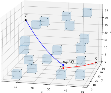
Figure 7: Output of the planner MASPA in a random scenario with $p=16$ and $q=30$. The marsupial system follows the ground path (red) from the starting point $S$ to the point $X$ avoiding obstacles. Then, from $top(X)$, the UAV is deployed and follows the collision-free aerial path (blue) with the shape of a catenary towards the target point $T$. In MASPA, the point $X$ is selected to minimize the sum of the lengths of the ground and aerial paths.

VIII Experimental Evaluation

In this section, we test the application of MASPA in realistic scenarios and compare it with a baseline method . First, we design two realistic scenarios where obstacles are selected in a structured way. Next, we propose a baseline method based on the RRT* technique to find solutions to these scenarios and compare them with MASPA. Furthermore, we measure the effect of the visibility module (PVA) in MASPA.

VIII-A RRT* Baseline

Due to the lack of studies on sequential marsupial planning, we implement a baseline method based on the well-known RRT* algorithm for path planning [16] and compare the results with MASPA. The RRT* algorithm is a provably asymptotically optimal method that randomly samples feasible states in the space and connects them into a tree graph, such that the edges of the graph minimize a certain cost function. RRT* is popularly used in problems with dynamic constraints to create the shortest path between initial and ending states while avoiding collisions with obstacles.

For the sake of comparison, we utilize RRT* to generate collision-free paths on the ground from the starting point $S$ for the UGV. In this scenario, each node in the RRT* tree represents a position on the ground that the UGV can reach without collisions. For each node $X$ on the ground, we check if the point $top(X)$ is $c_{L}$-visible and, if so, compute the minimum aerial path to $T$ using the CVP algorithm described in Section VI. Finally, we select the node $X$ in the tree that minimizes the sum of the path length from $X$ to $S$ and the path length from $top(X)$ to $T$. If no such point exists, we conclude that there is no feasible solution to the problem.

As a stopping parameter in the RRT* algorithm, we consider the maximum resolution time. This parameter defines how long the RRT* algorithm runs to create random points. The longer the algorithm runs, the more random points are generated, increasing the likelihood of obtaining a good solution. However, a poor selection of this parameter can lead to suboptimal solutions or, in some cases, to no solution at all.

VIII-B Comparison

In this section, we compare the baseline approach based on RRT* with MASPA in the following two realistic scenarios:

• S1 (Fireplace): This scenario involves a system of walls that simulate a fireplace. The target $T$ is located above the fireplace hole. The marsupial system must enter the enclosure and deploy the UAV through the fireplace to reach $T$, Figure 8.

• S2 (Balconies): This scenario involves a building with two balconies, each occupied by a person who needs help. The marsupial system must plan a path to reach both balconies sequentially. Additionally, there is a designated forbidden area around the building that the UGV must avoid, as illustrated in Figure 9. This scenario is challenging because the UAV can access the target points only through a small gap in the balconies, as shown in Figure 9 (c).

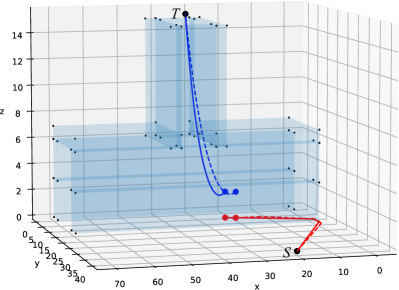
Figure 8: Resulting path in scenario S1 (Fireplace) for the MASPA strategy with $p=16$ and $q=30$, compared to the RRT* baseline executed for 20 seconds. The dashed lines represent the ground and aerial paths retrieved by the RRT* algorithm.

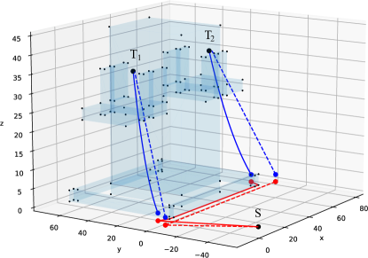
(a)

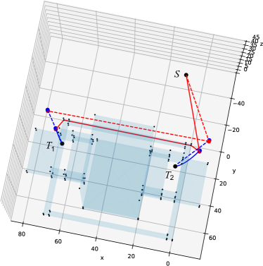
(b)

Figure 9: Resulting paths in scenario S2 (Balconies) for the MASPA strategy with $p=16$ and $q=30$, compared to the RRT* baseline, executed for 20 seconds. The dashed lines represent both the ground and aerial paths retrieved by the RRT* algorithm. Top view at the bottom.

In the S1 and S2 scenarios, we use the MASPA strategy with parameter values $p=16$ and $q=30$, selected based on the parameter study in Section VII. For RRT*, we set the maximum resolution time parameter to 20 seconds. This duration was chosen because lower values of this parameter resulted in poor solutions and, in some cases, no solutions were found.

In scenario S2, the goal is to compute a path for the marsupial robotics system to sequentially visit two targets, and we use the planners twice, consecutively and independently. First, we compute the optimal path from the starting point to the first target. After reaching it, we assume that the UAV returns to the UGV by retracing its collision-free aerial path. Finally, we plan a path from the UGV’s current position to the second target. This scenario is particularly challenging because finding optimal solutions requires the UAV to navigate through the gaps beneath each balcony. In contrast, a suboptimal approach tends to take a longer route that flies directly to the target, passing above the balconies.

Finally, in order to validate the use of the visibility module, we include a third approach, which is the MASPA strategy without the visibility algorithm, referred to as MASPA^-. This variant does not use PVA to filter non $c_{L}$-visible points. Instead, it considers candidates for take-off points that are uniformly located along the straight line $r_{top}$. Table III presents the results of the comparison between the three planners in terms of total path lengths. Both the MASPA and MASPA^- strategies are deterministic, which means that they will produce the same output given the same input and parameters. In contrast, the RRT* baseline incorporates a random component, so we run the algorithm 10 times and report the mean and standard deviation of the results in the table. As shown, MASPA outperforms the RRT* baseline after 20 seconds of execution.

TABLE III: Mean and standard deviation values (in meters) for the TL metric across the different planners.

Scenario	MASPA	MASPA-	RRT*
S1 (Fireplace)	$78.0$	$78.0$	$85.3\pm 3.5$
S2 (Balconies)	$314.8$	$314.8$	$372.4\pm 47.9$

Table IV presents the results of the comparison between the three planners in terms of total execution time. The RRT * baseline runs for 20 seconds, resulting in a total of 40 seconds for scenario S2, due to the need for two consecutive planning runs. The table illustrates the significant advantage of using the visibility module, which drastically reduces the execution time of the MASPA strategy, making it at least four times faster in both scenarios, which is of great value in emergency scenarios. In particular, the execution time of MASPA could be further reduced with a more efficient implementation, such as one in a faster language like C or C++, compared to Python. In view of these results, we conclude that MASPA outperforms RRT* in both metrics, especially in scenarios with nooks and crannies where visibility with a catenary is low.

TABLE IV: Values (in seconds) for the ET metric across the different planners.

Scenario	MASPA	MASPA-	RRT*
S1 (Tunnel)	$0.5$	$4.4$	$20$
S2 (Building)	$3.2$	$14.1$	$40$

As an additional test, we ran the RRT* baseline algorithm for scenario S1 with unlimited execution time to determine how long it would take to find a better solution than MASPA. The baseline approach ultimately found a solution with a path shorter than MASPA after 18 minutes of computation. This result underscores the substantial impact of addressing the visibility problem for planning tasks with a marsupial robotics system.

IX Conclusion and Future Work

An heterogeneous marsupial robotics system uses different types of robots to expand their operation envelope, leveraging the unique strengths of each robot. This paper introduces the planner MASPA, a novel algorithm for optimal path planning in autonomous marsupial systems. The method computes efficient paths online for specific parameter settings. MASPA incorporates a visibility module, PVA, to avoid a time-consuming brute-force approach. This module identifies a discrete set of feasible take-off points after computing maximal visible intervals in the take-off line within a vertical plane. We have demonstrated the effectiveness of MASPA in both random and realistic scenarios, with experimental results showing that MASPA outperforms a competitive path planning baseline based on RRT* in terms of both total path length and execution time. An open-source implementation of both MASPA and the baseline is available online .

As future work, we anticipate several potential extensions for MASPA, which we discuss in the following:

• 3D Visibility Area for Taut Tethers: Compute the area in the take-off plane $\pi_{top}$ of feasible $p_{L}$-visible points. Specifically, determine the exact locus on the plane of points from which the target $T$ can be reached with a taut tether of length at most $L$.

• Visibility with Catenaries (2D and 3D): We consider the problem of computing the exact locus of $c_{L}$-visible points an interesting open challenge. Solving this problem efficiently could enable a more precise discrimination of non $c_{L}$-visible take-off points compared to the PVA proposed in this work. An exact algorithm for this problem could reduce the execution time and improve the path lengths. Furthermore, computing the exact locus of $c_{L}$-visible points in the 3D space could potentially solve the open problem of finding the optimal solution for SMPP with an efficient and exact algorithm.

• Sequential Targets: In scenario S2, we observed the importance of planning sequential paths for multiple target points. In this work, we addressed this problem by planning paths to one target at a time. An interesting extension would be to develop a method that simultaneously optimizes the path for the marsupial to visit all target points.

• Simultaneous Planning: Related to the previous point, another open problem is computing a feasible solution for both the UGV and the UAV considering their simultaneous movement. In this scenario, the UAV would need to visit a set of targets sequentially, while the UGV would have to follow the UAV, ensuring that the paths adhere to the maximum tether length constraint. This problem involves coordinating the movements of both vehicles to optimize the overall path while respecting the length limits of the tether.

• Field Experimentation: Finally, we plan to apply MASPA to compute trajectories for a real marsupial robotics system prototype. To achieve this, we will integrate the planner with controllers for flight stabilization and trajectory tracking [45], ensuring the practical implementation of the proposed algorithm in real-world scenarios.

References

- [1] David Alejo, François Chataigner, Daniel Serrano, Luis Merino, and Fernando Caballero. Into the dirt: Datasets of sewer networks with aerial and ground platforms. Journal of Field Robotics, 38(1):105–120, 2021.
- [2] Javier Alonso-Mora, Tobias Naegeli, Roland Siegwart, and Paul Beardsley. Collision avoidance for aerial vehicles in multi-agent scenarios. Autonomous Robots, 39(1):101–121, 2015.
- [3] Barbara Arbanas, Frano Petric, Ana Batinović, Marsela Polić, Ivo Vatavuk, Lovro Marković, Marko Car, Ivan Hrabar, Antun Ivanović, and Stjepan Bogdan. From ERL to MBZIRC: Development of An Aerial-Ground Robotic Team for Search and Rescue. In Elmer P. Dadios, editor, Automation and Control, chapter 4. IntechOpen, 2021.
- [4] Mauricio Aristizabal, José L Hernández-Estrada, Manuel Garcia, and Harry Millwater. Solution and sensitivity analysis of nonlinear equations using a hypercomplex-variable newton-raphson method. Applied Mathematics and Computation, 451:127981, 2023.
- [5] Takao Asano, Tetsuo Asano, Leonidas Guibas, John Hershberger, and Hiroshi Imai. Visibility-polygon search and euclidean shortest paths. In 26th annual symposium on foundations of computer science (SFCS 1985), pages 155–164. IEEE, 1985.
- [6] Michele Bolognini, Danilo Saccani, Fabrizio Cirillo, and Lorenzo Fagiano. Autonomous navigation of interconnected tethered drones in a partially known environment with obstacles. In IEEE Conference on Decision and Control (CDC), pages 3315–3320, 2022.
- [7] Andrea Borgese, Dario C. Guastella, Giuseppe Sutera, and Giovanni Muscato. Tether-based localization for cooperative ground and aerial vehicles. IEEE Robotics and Automation Letters, 7(3):8162–8169, 2022.
- [8] Muqing Cao, Kun Cao, Shenghai Yuan, Thien-Minh Nguyen, and Lihua Xie. Neptune: Nonentangling trajectory planning for multiple tethered unmanned vehicles. IEEE Transactions on Robotics, pages 1–19, 2023.
- [9] Y. Chen, M. Cutler, and J. P. How. Decoupled multiagent path planning via incremental sequential convex programming. In IEEE International Conference on Robotics and Automation (ICRA), pages 5954–5961, May 2015.
- [10] Chris Dinelli, John Racette, Mario Escarcega, Simon Lotero, Jeffrey Gordon, James Montoya, Chase Dunaway, Vasileios Androulakis, Hassan Khaniani, Sihua Shao, Pedram Roghanchi, and Mostafa Hassanalian. Configurations and applications of multi-agent hybrid drone/unmanned ground vehicle for underground environments: A review. Drones, 7(2), 2023.
- [11] Mohamed Elbanhawi and Milan Simic. Sampling-based robot motion planning: A review. IEEE Access, 2:56–77, 2014.
- [12] Aleksandra Faust, Ivana Palunko, Patricio Cruz, Rafael Fierro, and Lydia Tapia. Automated aerial suspended cargo delivery through reinforcement learning. Artificial Intelligence, 247:381–398, 2017.
- [13] Hamido Hourani, Philipp Wolters, Eckart Hauck, and Sabina Jeschke. A marsupial relationship in robotics: A survey. In Sabina Jeschke, Ingrid Isenhardt, Frank Hees, and Klaus Henning, editors, Automation, Communication and Cybernetics in Science and Engineering 2011/2012, pages 667–679. Springer Berlin Heidelberg, Berlin, Heidelberg, 2013.
- [14] Nicolas Hudson, Fletcher Talbot, Mark Cox, Jason Williams, Thomas Hines, Alex Pitt, Brett Wood, Dennis Frousheger, Katrina Lo Surdo, Thomas Molnar, et al. Heterogeneous ground and air platforms, homogeneous sensing: Team CSIRO Data61’s approach to the DARPA subterranean challenge. arXiv preprint arXiv:2104.09053, 2021.
- [15] S. Karaman and E. Frazzoli. Sampling-based algorithms for optimal motion planning. The International Journal of Robotics Research, 30(7):846–894, 2011.
- [16] Sertac Karaman and Emilio Frazzoli. Sampling-based algorithms for optimal motion planning. The international journal of robotics research, 30(7):846–894, 2011.
- [17] O Lopez-Garcia, A Carnicero, and V Torres. Computation of the initial equilibrium of railway overheads based on the catenary equation. Engineering structures, 28(10):1387–1394, 2006.
- [18] Carlos E. Luis and Angela P. Schoellig. Trajectory generation for multiagent point-to-point transitions via distributed model predictive control. IEEE Robotics and Automation Letters, 4(2):375–382, 2019.
- [19] Sergei Lupashin and Raffaello D’Andrea. Stabilization of a flying vehicle on a taut tether using inertial sensing. In 2013 IEEE/RSJ International Conference on Intelligent Robots and Systems, pages 2432–2438. IEEE, 2013.
- [20] H. Ma, D. Harabor, P. J. Stuckey, J. Li, and S. Koenig. Searching with consistent prioritization for multi-agent path finding. In AAAI Conference on Artificial Intelligence, pages 7643–7650, 2019.
- [21] Hang Ma, Wolfgang Hoenig, T. K. Satish Kumar, Nora Ayanian, and Sven Koenig. Lifelong path planning with kinematic constraints for multi-agent pickup and delivery. In AAAI Conference on Artificial Intelligence, pages 7651–7658, 2019.
- [22] Bernardo Martinez Rocamora Jr, Rogério R Lima, Kieren Samarakoon, Jeremy Rathjen, Jason N Gross, and Guilherme AS Pereira. Oxpecker: A tethered UAV for inspection of stone-mine pillars. Drones, 7(2):73, 2023.
- [23] Simón Martinez-Rozas, David Alejo, Fernando Caballero, and Luis Merino. Path and trajectory planning of a tethered UAV-UGV marsupial robotic system. IEEE Robotics and Automation Letters, 2023.
- [24] S. Martínez-Rozas, D. Alejo, F. Caballero, and L. Merino. Optimization-based trajectory planning for tethered aerial robots. In IEEE International Conference on Robotics and Automation (ICRA), pages 362–368, 2021.
- [25] Takahiro Miki, Petr Khrapchenkov, and Koichi Hori. UAV/UGV Autonomous Cooperation: UAV assists UGV to climb a cliff by attaching a tether. In International Conference on Robotics and Automation (ICRA), pages 8041–8047, 2019.
- [26] Robin R Murphy, Michelle Ausmus, Magda Bugajska, Tanya Ellis, Tonia Johnson, Nia Kelley, Jodi Kiefer, and Lisa Pollock. Marsupial-like mobile robot societies. In Proceedings of the third annual conference on Autonomous Agents, pages 364–365, 1999.
- [27] Alex Nash, Sven Koenig, and Craig Tovey. Lazy Theta*: Any-Angle Path Planning and Path Length Analysis in 3D. In AAAI Conference on Artificial Intelligence, pages 147–154, 2010.
- [28] Christos Papachristos and Anthony Tzes. The power-tethered UAV-UGV team: A collaborative strategy for navigation in partially-mapped environments. In Mediterranean Conference on Control and Automation, pages 1153–1158, 2014.
- [29] Louis Petit and Alexis Lussier Desbiens. TAPE: Tether-aware path planning for autonomous exploration of unknown 3D cavities using a tangle-compatible tethered aerial robot. IEEE Robotics and Automation Letters, 7(4):10550–10557, 2022.
- [30] F. Real, A. R. Castaño, A. Torres-Gonzalez, J. Capitan, P. J. Sanchez-Cuevas, M. J. Fernandez, H. Romero, and A. Ollero. Autonomous fire-fighting with heterogeneous team of unmanned aerial vehicles. Field Robotics, 1:158–185, 2021.
- [31] Tomás Roucek, Martin Pecka, Petr Cízek, Tomás Petrícek, Jan Bayer, Vojtech Salanský, Teymur Azayev, Daniel Hert, Matej Petrlík, Tomás Báca, Vojtech Spurný, Vít Krátký, Pavel Petrácek, Dominic Baril, Maxime Vaidis, Vladimír Kubelka, François Pomerleau, Jan Faigl, Karel Zimmermann, Martin Saska, Tomás Svoboda, and Tomás Krajník. System for multi-robotic exploration of underground environments CTU-CRAS-NORLAB in the DARPA subterranean challenge. ArXiv e-prints, 2021.
- [32] Luis A Sandino, Daniel Santamaria, Manuel Bejar, Antidio Viguria, Konstantin Kondak, and Anibal Ollero. Tether-guided landing of unmanned helicopters without GPS sensors. In 2014 IEEE International Conference on Robotics and Automation (ICRA), pages 3096–3101. IEEE, 2014.
- [33] Guillaume Sartoretti, Justin Kerr, Yunfei Shi, Glenn Wagner, T. K. Satish Kumar, Sven Koenig, and Howie Choset. PRIMAL: Pathfinding via Reinforcement and Imitation Multi-Agent Learning. IEEE Robotics and Automation Letters, 4(3):2378–2385, 2019.
- [34] Guni Sharon, Roni Stern, Ariel Felner, and Nathan R. Sturtevant. Conflict-based search for optimal multi-agent pathfinding. Artificial Intelligence, 219:40–66, 2015.
- [35] Paul G. Stankiewicz, Stephen Jenkins, Galen E. Mullins, Kevin C. Wolfe, Matthew S. Johannes, and Joseph L. Moore. A motion planning approach for marsupial robotic systems. In International Conference on Intelligent Robots and Systems (IROS), pages 1–9, 2018.
- [36] Marco Tognon and Antonio Franchi. Theory and Applications for Control of Aerial Robots in Physical Interaction Through Tethers. Springer Cham, 2020.
- [37] Jesus Tordesillas and Jonathan P. How. Mader: Trajectory planner in multiagent and dynamic environments. IEEE Transactions on Robotics, 38(1):463–476, 2022.
- [38] Carlos Viegas, Babak Chehreh, Jose Andrade, and Joao Lourenço. Tethered UAV with combined multi-rotor and water jet propulsion for forest fire fighting. Journal of Intelligent & Robotic Systems, 104(21), 2022.
- [39] Chao Wang, Jian Wang, Yuan Shen, and Xudong Zhang. Autonomous navigation of uavs in large-scale complex environments: A deep reinforcement learning approach. IEEE Transactions on Vehicular Technology, 68(3):2124–2136, 2019.
- [40] Hanfu Wang and Weidong Chen. Multi-robot path planning with due times. IEEE Robotics and Automation Letters, 7(2):4829–4836, 2022.
- [41] Wenying Wu, Subhrajit Bhattacharya, and Amanda Prorok. Multi-robot path deconfliction through prioritization by path prospects. In IEEE International Conference on Robotics and Automation (ICRA), pages 9809–9815, 2020.
- [42] Xuesu Xiao, Jan Dufek, and Robin Murphy. Benchmarking tether-based UAV motion primitives. In IEEE International Symposium on Safety, Security, and Rescue Robotics (SSRR), pages 51–55, 2019.
- [43] Xuesu Xiao, Jan Dufek, and Robin R. Murphy. Tethered aerial visual assistance. ArXiv e-prints, 2020.
- [44] Xuesu Xiao, Jan Dufek, and Robin R Murphy. Autonomous visual assistance for robot operations using a tethered UAV. In Field and Service Robotics: Results of the 12th International Conference, pages 15–29. Springer, 2021.
- [45] Lin-Xing Xu, Yu-Long Wang, Fei Wang, and Yue Long. Event-triggered active disturbance rejection trajectory tracking control for a quadrotor unmanned aerial vehicle. Applied Mathematics and Computation, 449:127967, 2023.
- [46] J. Yu and S. M. LaValle. Optimal multirobot path planning on graphs: Complete algorithms and effective heuristics. IEEE Transactions on Robotics, 32(5):1163–1177, Oct 2016.
- [47] Hai Zhu and Javier Alonso-Mora. Chance-constrained collision avoidance for MAVs in dynamic environments. IEEE Robotics and Automation Letters, 4(2):776–783, 2019.