Investigating the hyperparameter space of deep neural network models for reaction coordinate optimization: Application to alanine dipeptide in water

Abstract

Identifying reaction coordinates (RCs) from many collective variable candidates have been of great challenge in understanding reaction mechanisms in complex systems. Machine learning approaches, especially the deep neural network (DNN), have become a powerful tool and are actively applied. On the other hand, selecting the hyperparameters that define the DNN model structure remains to be a nontrivial and tedious task. Here we develop the hyperparameter tuning approach to determine the parameters in an automatic fashion from the trajectory data. The DNN models are constructed to obtain a RC from many collective variables that can adequately describe the changes of the committor from the reactant to product. The approach is applied to study the isomerization of alanine dipeptide in vacuum and in water. We find that multiple DNN models with similar accuracy can be obtained, indicating that hyperparameter space is multimodal. Nevertheless, despite the differences in the DNN model structure, the key features extracted using the explainable AI (XAI) tools show that all RC share the same character. In particular, the reaction in vacuum is characterized by the dihedral angles $\phi$ and $\theta$. The reaction in water also involves these dihedral angles as key features, and in addition, the electrostatic potential from the solvent to the hydrogen (H₁₈) plays a role at about the transition state. The current study thus shows that, in contrast to the diversity in the DNN models, suitably optimized DNN models share the same features and share the common mechanism for the reaction of interest.

I Introduction

Transition state (TS) plays a fundamental role in chemical reactions and enzyme catalysis.Pauling (1948); Wolfenden (1969); Schramm (2007); Jiang et al. (2008); Peters (2017) While reactions in simple model system can be well characterized using a few TSs, the reactions in solution and biomolecules involve numerous intermediate and TSs on the high-dimensional potential energy surface.Bruice (2002); Garcia-Viloca et al. (2004); Ishida and Kato (2003); Hayashi et al. (2012); Masgrau and Truhlar (2015) It is thus indispensable to describe the reactions on the low-dimensional free energy surface (FES) described by a few collective variables (CVs), and it has been of great interest to determine the optimal CVs from a number of possible CV candidates that can adequately describe the FES and TS. In a representative case of alanine dipeptide, the conformational transitions have been successfully characterized with the FES using two dihedral angles, $\phi$ and $\psi$, known as the Ramachandran plotRamachandran and Sasisekharan (1968) (Figure 1).

From a kinetic perspective, TS is considered as a point in potential or free energy surface having equal probability of reaching the reactant and product states.Geissler, Dellago, and Chandler (1999); Hummer (2004); Peters (2016) The committor $p_{B}(\mathbf{x})$, defined as the probability of reaching the state $B$ from the configuration denoted by $\mathbf{x}$ without returning to state $A$, changes monotonically from 0 to 1 along an ideal RC and become 0.5 at the TS. $p_{B}$ thus serves as a good measure to evaluate the quality of a RC, and have been used to optimize the RCs from a large number of candidate CVs.Bolhuis, Dellago, and Chandler (2000); Rhee and Pande (2005); Ma and Dinner (2005); Peters, Beckham, and Trout (2007); Jung et al. (2023); Quaytman and Schwartz (2007); Branduardi, Gervasio, and Parrinello (2007); Peters, Beckham, and Trout (2007); Mullen, Shea, and Peters (2014); Okazaki et al. (2019); Mori and Saito (2020); Mori et al. (2020); Wu, Li, and Ma (2022a, b); Manuchehrfar et al. (2021); Zhang et al. (2024) These studies of RCs have led to realize that an adequate RC that satisfies the $p_{B}\sim 0.5$ condition is often much more complicated than typical CVs used to build the FESsMa and Dinner (2005); Mullen, Shea, and Peters (2014); Mori et al. (2013). For instance, in the case of alanine dipeptide, the $C_{\mathrm{eq}}$ to $C_{\mathrm{ax}}$ transition in vacuum required another dihedral angle $\theta$ (Figure 1)Bolhuis, Dellago, and Chandler (2000), and the reaction in water is even more complex.Bolhuis, Dellago, and Chandler (2000); Ma and Dinner (2005)

Machine learning (ML) approaches have recently been actively applied to identify the CVs and RCs from the molecular dynamics (MD) simulation trajectoriesMardt et al. (2018); Chen and Ferguson (2018); Sultan and Pande (2018); Ribeiro et al. (2018); Rogal, Schneider, and Tuckerman (2019); Wang, Ribeiro, and Tiwary (2020); Bonati, Rizzi, and Parrinello (2020); Belkacemi et al. (2021); Bonati, Piccini, and Parrinello (2021); Hooft, Ortíz, and Ensing (2021); Frassek, Arjun, and Bolhuis (2021); Zhang et al. (2021); Kikutsuji et al. (2022); Neumann and Schwierz (2022); Liang et al. (2023); Lazzeri et al. (2023); Singh and Limmer (2023); Jung et al. (2023); Ray, Trizio, and Parrinello (2023); Naleem et al. (2023); Majumder and Straub (2024). In particular, Ma and DinnerMa and Dinner (2005) have developed an automatic CV search algorithm by combining the genetic algorithm to identify the RC for the alanine dipeptide isomerization. Along this line, we have recently combined the deep neural network (DNN) approach with the cross-entropy minimization methodMori and Saito (2020); Mori et al. (2020) to optimize the RC from many CV candidates using the committor distribution as a measureKikutsuji et al. (2022); Okada et al. (2024). Our study highlighted the effectiveness of the explainable AI (XAI) method in characterizing the CVs that contribute to the RC.

While DNN approach can be very powerful in describing the non-linear contributions of CVs to RC, the structure of the DNN model determined by the hyperparameters, e.g. the number of layers and nodes per layer, is highly flexible and are often chosen intuitively. Yet, the adequacy of the hyperparameters remain ambiguous.

In this regard, Neumann and SchwierzNeumann and Schwierz (2022) have recently applied the Keras Tuner random search hyperparameter optimization to automatically determine the DNN model that can describe the committor of the magnesium binding to RNA. Yet, how the choice of hyperparameters affects the quality of the DNN model and the outcome remains unclear. The applications of DNN models thus suffer from determining the appropriate hyperparameters, which remains to be highly tedious and nontrivial task.

To this end, here we develop a hyperparameter tuning approach by applying the Bayesian optimization methodWu et al. (2019) to determine the DNN model for RC optimization in an automatic manner. The method takes the committors and large number of candidate CVs as the input without pre-determined the hyperparameters for the DNN model, and automatically determines the appropriate DNN model and the RC. To illustrate its performance, we apply this approach to alanine dipeptide isomerization in vacuum and in water. The reaction in vacuum serves as a test case to explore the robustness of the hyperparameters, whereas that in water showcases the effectiveness of the method in a more complex case where solvent plays a role.

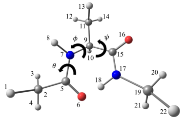
Figure 1: Alanine dipeptide with atom indexes. The three key dihedral angles, i.e., $\phi$, $\psi$, and $\theta$, the dihedral angles about the C₅-N₇, N₇-C₉, and C₉-C₁₅ bonds, respectively, are also shown.

II Methods

II.1 Committor and Cross Entropy function

Committor $p_{B}(\mathbf{x})$ describes the probability of a trajectory generated from $\mathbf{x}$ to reach the product state $B$. Along a RC $q$, $p_{B}$ is expected to change smoothly from 0 to 1 and becomes 0.5 at the transition state. The ideal committor value at $q$, $f_{B}(q)$, can thus be described by a sigmoidal function, $f_{B}(q)=\left(1+\tanh(q)\right)/2$.

When the data point $k$ is characterized by the collective variables (CVs) $\mathbf{x}^{(k)}$ and committor $p_{B}^{(k)}$, the discrepancy between the ideal value and raw committor data can be described by the cross-entropy functionMori and Saito (2020); Mori et al. (2020)

$$\mathcal{H}(q)=-\sum_{k}{}p_{B}^{(k)}\log f_{B}(q^{(k)})-\sum_{k}{}\left(1-p_{B}^{(k)}\right)\log\left\{1-f_{B}(q^{(k)})\right\}$$ (1)

Here, $k$ denotes the data points and $q^{(k)}$ is the RC as a function of $\mathbf{x}^{(k)}$. Eq. 1 is derived from the Kullback-Leibler divergenceMori and Saito (2020), which quantifies the mismatch between the distribution of the raw ($p_{B}^{(k)}$) and expected ($f_{B}(q^{(k)})$) committors. It is also noted that Eq. 1 is a generalization of the maximum-likelihood function used with aimless shooting algorithmPeters, Beckham, and Trout (2007).

By minimizing Eq. 1, one can optimize $q^{(k)}$ to minimize the difference between $p_{B}$ and $f_{B}(q^{(k)})$. In practice, we employ the $L_{2}$ regularization function to suppress overfitting. The regularization lambda $\lambda$ is set separately for each layer (see below).

II.2 Deep neural network model

The DNN function converts the CVs $\mathbf{x}^{(k)}$ into a RC $q^{(k)}$ in a non-linear manner. Here we adopt the multilayer perceptron model which consists of the input layer $\mathbf{x}^{(k)}$, multiple hidden layers with different number of nodes, and the output layer $q^{(k)}$ (Figure 2). The CVs are standardized prior to constructing $\mathbf{x}^{(k)}$. The leaky rectified linear unit (Leaky ReLU) with a leaky parameter set of 0.01 was used for the activation function. The $L_{2}$ regularization was employed, where $\lambda$ was varied in the hyperparameter tuning step. Note that different $\lambda$ was used for each layer. The numbers of hidden layers and nodes in each layer, N_layer and ${\mathbf{N}}_{\mathrm{node}}$, respectively, are also the hyperparameters that are left to be explored. Optimization was performed using AdaMax. The learning rate lr and two decay factors $\beta_{1}$ and $\beta_{2}$ were set to the default values of 0.001, 0.9, and 0.99, respectively. The TensorFlowAbadi et al. (2015) library was used to implement the DNN model.

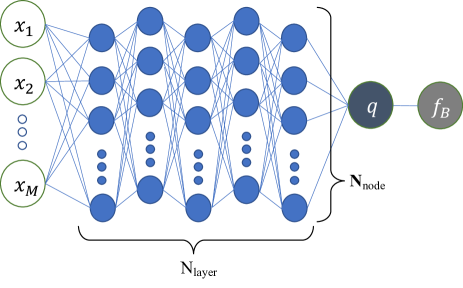
Figure 2: Overview of the multilayer perception model used in this work. The input CVs ($x_{i}$) are converted to the output ($q$) with a DNN model of N_layer consisting of ${\mathbf{N}}_{\mathrm{node}}$. $f_{B}$ is the predicted $p_{B}$ value at $q$ described by a sigomidal function ($f_{B}(q)=(1+\tanh(q))/2$).

II.3 Hyperparameter tuning and DNN model optimization

The hyperparameters in the current DNN, N_layer, ${\mathbf{N}}_{\mathrm{node}}$, and $\lambda$, are not unique and can strongly affect the performance of the DNN model. Here we employ the hyperparameter tuning approach using the Bayesian optimization method to determine these parameters in an automatic manner.

The hyperparameter tuning and DNN model optimization are performed in two stages. First, the data is divided into training and validation set at a ratio of 8:2. N_layer is searched between 2 and 5, and ${\mathbf{N}}_{\mathrm{node}}$ are explored separately for each layer, which are chosen within the range from 100 to 5000 in 100 increments. $\lambda$ is explored between 0.0001 to 0.100 with 20 points equally spaced in logarithmic scale. The initial values for these parameters are chosen randomly within the exploration range. Bayesian optimization was performed for 150 trials, where the DNN model for each hyperparameter was trained for a maximum of 1000 epochs using Eq. 1. Early stopping was applied when the value of loss function for the validation set did not improve for 5 consecutive steps. The performance of the model at each step was evaluated using the root-mean-square error (RMSE) for the validation set, calculated as a difference between the predicted and reference $p_{B}$. After the optimal choice of the parameters are determined, the data are unified and re-partitioned into training, validation, and test sets at a ratio of 5:1:4, and the DNN model is optimized for 1000 epochs with the same criteria for Early Stopping. The Keras TunerO’Malley et al. (2019) library was used to implement the DNN model.

II.4 DNN model interpretation with LIME and SHAP

To interpret the DNN model, the Local Interpretable Model-agnostic Explanation (LIME)10. (2016) and SHapley Additive exPlanations (SHAP)Lundberg and Lee methods were applied to the data. In brief, LIME builds a linear regression function to explain the local behavior of the target data from the perturbation of input variables, whereas SHAP employs an additive feature attribution method that ensures fair distribution of predictions among input features in accordance with the game-theory-based Shapley value. LimeTabularExplainer for LIME and DeepExplainer for SHAP were employed, using the packages obtained from https://github.com/marcotcr/lime and https://github.com/slundberg/shap, respectively.

II.5 Conformational sampling of alanine dipeptide

The initial structures of alanine dipeptide in vacuum and water were generated using AmberTools21Case et al. . In the case in water, alanine dipeptide was solvated in a rectangular parallelepiped box with 1683 water molecules. Alanine dipeptide and water were treated with the Amber14SB force field and TIP3P model, respectively. The system was energy minimized for 3000 steps and heated up to 300 K in 50 ps. MD simulations under NPT and NVT conditions were then performed for 100 and 1000 ps, respectively, to complete equilibration.

Umbrella sampling (US) and transition path sampling (TPS) were combined to collect broad conformations about the transition path of alanine dipeptide in vacuum and water as follows. First, the transition state region (i.e., $\phi\sim$ 0) was sampled using the US along $\phi$ with a force constant of 100.0 kcal mol^-1 rad^-2 while restraining $\psi$ to $\psi\leq 0^{\circ}$ with a half-harmonic potential with a force constant of 10.0 kcalmol^-1 rad^-2 (See Figure 1 for definitions of $\phi$ and $\psi$). 100 conformations from the 10 ns-long trajectory with the harmonic restraint centered at $\phi=0.0$ was then evenly collected. From each conformation, 10 trajectories of 2 ps long were generated by sampling the initial velocity from the Maxwell-Boltzmann distribution at 300 K and propagating the trajectory for 1 ps forward and backward in time under the NVE condition. States A and B were defined as $\phi\leq-30$ and $\phi\geq 30$, respectively. It is noted that while the previous studiesMa and Dinner (2005); Bolhuis, Dellago, and Chandler (2000) have often studied the C_7eq $\rightarrow$ $\alpha_{\mathrm{R}}$ transitions in solution, which have lower energy barrierAnderson and Hermans (1988), here we focus on the isomerization about $\phi$ to compare the results in vacuum and water.

From the successful transition trajectories which connect states A and B, new points were generated by extracting snapshots within 0.1 ps from the time origin of each trajectory. The velocity for each point was sampled from the Maxwell-Boltzmann distribution at 300 K, and a new ensemble of 2 ps-long trajectories were generated following the same procedure as above. Roughly 33 and 42 % of the trial trajectories were accepted throughout the TPS of alanine dipeptide in vacuum and water, respectively. After the 3rd round, 3,714 and 4,590 points were generated for the following committor calculations in vacuum and in water.

From each data point after the final round of TPS, 2 ps-long trajectories were generated 100 times per point with velocities randomly sampled from the Maxwell-Boltzmann distribution at 300 K. $p_{B}$ was calculated by $p_{B}=n_{B}/(n_{A}+n_{B})$ where $n_{I}$ denotes the number of trajectories that is at state $I$ at the end of the trajectory. The data points projected on the ($\phi$, $\psi$) plane, with colors describing the $p_{B}$ value, are shown in Figure 3. We note that the data points were obtained over a broader range of $\phi$ compared to those sampled with the aimless shooting algorithmMori et al. (2020). As a consequence, the $p_{B}$-distribution were not even, especially in vacuum where roughly half of the points were found in either $p_{B}\leq 0.1$ or $p_{B}\geq 0.9$. Here we note that the minima on the $\phi<0$ side in water, corresponding to the $\alpha_{\mathrm{R}}$ state, is located at $\psi<0$Ma and Dinner (2005); Anderson and Hermans (1988). The transition path in water is thus also located on the $\psi<0$ side compared to that in vacuum.

The collective variables (CVs) are listed in Supplementary material Table S1, and the atom indexes are given in Figure 1.

All MD simulations were performed using Amber 20 software packageCase et al. ; Salomón-Ferrer et al. (2013).

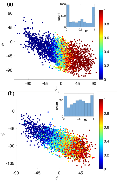
Figure 3: Distributions of the data points in ($\phi$,$\psi$) space from the trajectories in (a) vacuum and (b) water. Colors represent the calculated $p_{B}$ data at each point. The insets in (a) and (b) show the committor distributions for all the data points in vacuum and water, respectively.

III Results and discussion

III.1 Comparison of different hyperparameters

We first compare the results of hyperparameter tuning using the isomerzation reaction of alanine dipeptide in vacuum. 10 models were constructed using different initial seeds including data partitioning. The CV candidates consist of 45 dihedral angles in cosine and sine forms, i.e., 90 variables, which follow our previous works.Mori et al. (2020); Kikutsuji et al. (2022) The convergence of the objective function $\mathcal{L}$, given in Fig.4, shows that the optimizations are converged within 60 to 100 epochs. Since further extending the number of epochs leads to slightly decreases $\mathcal{L}$ for the training data but increases that for the validation data, we find that these epoch numbers are sufficient for suppressing overfitting and maximizing predictability. The obtained hyperparameters are summarized in Table 1. Surprisingly, the number of layers (N_layer) and nodes (${\mathbf{N}}_{\mathrm{node}}$) differ remarkably between the models. ${\mathbf{N}}_{\mathrm{node}}$ often converged to the maximum (5000) as well as the minimum (100), and ${\mathbf{N}}_{\mathrm{node}}$ = 5 was most frequently selected (5 out of 10 models). $\lambda$ was often found to be at the minimum (0.0001), especially in the first layer, but can be up to 0.0695 and varied between the layers. Overall, no apparent unique optimal model was obtained.

Table 1: Optimized hyperparameters in vacuum. $q_{i}$ denote the RC obtained for the $i$-th model.

	$q_{1}$	$q_{2}$	$q_{3}$	$q_{4}$	$q_{5}$	$q_{6}$	$q_{7}$	$q_{8}$	$q_{9}$	$q_{10}$
Nlayer	5	2	3	5	5	3	5	4	2	5
${\mathbf{N}}_{\mathrm{node}}$(1)	5000	4000	4000	3500	5000	1400	5000	4100	2700	5000
$\lambda$(1)	0.0001	0.0001	0.0001	0.1000	0.0001	0.0001	0.0001	0.0009	0.0001	0.0001
${\mathbf{N}}_{\mathrm{node}}$(2)	5000	5000	2500	5000	5000	5000	5000	2700	100	2100
$\lambda$(2)	0.0001	0.0113	0.0026	0.0001	0.1000	0.0001	0.0013	0.0018	0.0009	0.1000
${\mathbf{N}}_{\mathrm{node}}$(3)	5000	–	2900	100	4300	100	5000	3600	–	5000
$\lambda$(3)	0.0695	–	0.0001	0.0001	0.0001	0.0001	0.0001	0.0006	–	0.0026
${\mathbf{N}}_{\mathrm{node}}$(4)	3600	–	–	2400	100	–	5000	900	–	100
$\lambda$(4)	0.1000	–	–	0.0002	0.0001	–	0.1000	0.0002	–	0.0001
${\mathbf{N}}_{\mathrm{node}}$(5)	100	–	–	5000	5000	–	2000	–	–	5000
$\lambda$(5)	0.0001	–	–	0.0001	0.0001	–	0.0001	–	–	0.0001

To compare the accuracy of the coordinates from the perspective of $p_{B}$-predictability, the RMSE between the predicted and reference $p_{B}$ for the training and test data are shown in Fig. 5 for the 10 models. The RMSEs were within and around 0.005 for the training and test sets, respectively. Even the RMSEs for the data points about the TS ($-0.2<q_{i}<0.2$) are within 0.007 and 0.009 for the training and test data. These results indicate that while the optimized DNN models are not unique, the RCs show very similar quality, i.e., able to predict $p_{B}$ with similar accuracy. This implies that the hyperparameter space for the current DNN model is likely multimodal.

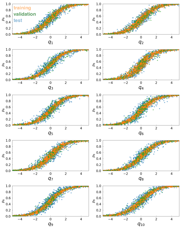
Figure S1: Scatter plots of the optimized coordinates ($q_{1}$ to $q_{10}$) and committors ($p_{B}$) in vacuum. Orange, green, and blue in (a) and (b) denote the results from the training, validation, and test data sets, respectively.

Figure 6 summarizes the change of $p_{B}$ along the first RC ($q_{1}$). Figure 6(a) shows that both training and test data closely follows the ideal sigmoidal line. The histogram of $p_{B}$ about the transition state (Figure 6(b)) indicates that both training and test data set shows a sharp peak at $p_{B}\sim 0.5$. These result implies that $q_{1}$ serves as a good RC and can clearly characterize the transition state. We note that similar results are obtained for the other RCs (Figs. S1 and S2).

Figure 7 summarizes the features that contribute to RC at about the TS extracted from LIME and SHAP. The extracted features are found to be very similar between the 10 RCs. CV₆₁, CV₅₈, and CV₅₄, corresponding to the sine form of $\phi$, $\phi$, and $\theta$, respectively, are the three major CVs in LIME analysis. The contribution of $\theta$ is increased in the SHAP analysis, but key CVs are unchanged from those found in LIME. The result is consistent with the previous studies which showed that $\theta$ becomes important at about the transition stateMa and Dinner (2005); Kikutsuji et al. (2022); Mori et al. (2020). On the other hand, the order as well as magnitude of the contributions are slightly different from those obtained in the previous XAI analysisKikutsuji et al. (2022). This may be due to the differences in the distribution of the data points where the current points are distributed over a broader range along $\phi$ (Figure 3).

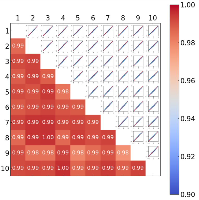
Figure S3: Scatter plots (top-right) and correlation coefficient (bottom-left) showing the correlation between the RCs from different optimized DNN models in vacuum. $q_{i}$ denote the optimized coordinate from the $i$-th DNN model. Note that all data points are included in these plots.

We also directly compared the RCs obtained from different DNN models by looking the scatter plots and correlation coefficients (Fig. S3). The result shows that every pair of RCs is highly correlated and the correlation coefficient is $>$0.99, indicating that despite the difference in the hyperparameters, the obtained RC are very similar. It is noted that the points at the negative and positive ends of the RCs where $p_{B}$ is 0 and 1, respectively, show slight deviations from the diagonal line in some of the plots. This is because $p_{B}$ is insensitive to the changes in the RCs at these ranges, and thus these points are not further optimized.

The current results show that while the optimization of DNN hyperparameters do not lead to a unique model, each DNN model produces equally good RCs showing similar predictability of $p_{B}$ and features that determine the TS.

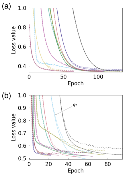
Figure 4: Training process of the loss function as a sum of the cross-entropy function and the $L_{2}$ regularization term in (a) vacuum and (b) water. Full and dashed lines show the values for training and validation data along the training process, and colors denote results for different models. Note that the training and data sets in each model are different due to different initial seed for data partitioning.

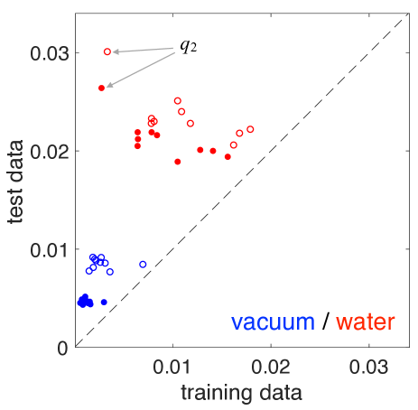
Figure 5: Scatter plot for RMSEs between the predicted and reference $p_{B}$ for the training and test data sets. Filled and open circles indicate the RMSEs using full points and those at about the TS ($-0.2<q_{i}<0.2$), respectively. Blue and red colors are the results in vacuum and water.

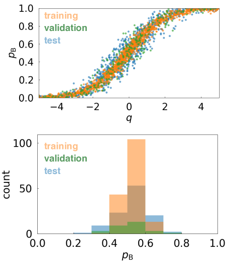
Figure 6: (a) Scatter plots of the optimized coordinate ($q$) and committor ($p_{B}$) for $q_{1}$ in vacuum. (b) Distribution of $p_{B}$ for the points within $-0.2<q_{1}<0.2$. Orange, green, and blue in (a) and (b) denote the results from the training, validation, and test data sets, respectively.

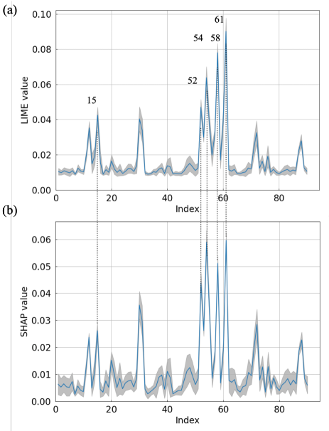
Figure 7: Contributions of CVs to the RCs in vacuum extracted using (a) LIME and (b) SHAP in absolute values. Blue lines and gray shades denote the average and variance calculated from the 10 RCs.

III.2 Application to alanine dipeptide in water

Next we apply the current approach to the isomerization of alanine dipeptide in water. Compared to the case in vacuum, the reaction in water has been a challenging task due to the contribution from the numerous waters surrounding the solute.Bolhuis, Dellago, and Chandler (2000) Previously, a complex CVs involving the torque have been proposed to be importantMa and Dinner (2005). Here we prefer to describe the solvation coordinates in a simple manner while preserving permutation invariance, and take account of the complex non-linear contribution through the DNN model. To this end, the electrostatic and van der Waals interaction from the waters to the atoms in alanine dipeptide were used as the CVs in addition to the intermolecular coordinates of alanine dipeptide (i.e., dihedral angles). Optimizations of the hyperparameters and DNN models were performed in the same manner as those in vacuum.

The optimized DNN models, summarized in Table 2, were again found to converge to different parameter sets. N_layer = 3 most frequently appeared, and ${\mathbf{N}}_{\mathrm{node}}$ were on average slightly smaller than those in vacuum. On the other hand, $\lambda$ were found to become larger than those in vacuum. This trend indicates that the increase in the number of CVs in water resulted in a slightly more compact model but with higher regularization penalty to suppress overfitting.

Table 2: Optimized hyperparameters in water. $q_{i}$ denote the RC obtained for the $i$-th model.

	$q_{1}$	$q_{2}$	$q_{3}$	$q_{4}$	$q_{5}$	$q_{6}$	$q_{7}$	$q_{8}$	$q_{9}$	$q_{10}$
Nlayer	3	5	3	3	5	2	3	2	3	5
${\mathbf{N}}_{\mathrm{node}}$(1)	100	4400	3800	2900	5000	1700	1300	2900	2300	5000
$\lambda$(1)	0.0001	0.0004	0.0013	0.0001	0.0001	0.0026	0.0009	0.0018	0.0001	0.0001
${\mathbf{N}}_{\mathrm{node}}$(2)	1200	1700	1600	5000	5000	100	800	100	5000	5000
$\lambda$(2)	0.1000	0.0162	0.0483	0.0079	0.0079	0.0018	0.1000	0.0234	0.0483	0.0055
${\mathbf{N}}_{\mathrm{node}}$(3)	3100	3800	1400	100	2000	–	3000	–	400	2500
$\lambda$(3)	0.0055	0.0004	0.0336	0.1000	0.1000	–	0.0018	–	0.0234	0.1000
${\mathbf{N}}_{\mathrm{node}}$(4)	–	800	–	–	5000	–	–	–	–	2000
$\lambda$(4)	–	0.0003	–	–	0.1000	–	–	–	–	0.1000
${\mathbf{N}}_{\mathrm{node}}$(5)	–	600	–	–	100	–	–	–	–	3700
$\lambda$(5)	–	0.0009	–	–	0.0001	–	–	–	–	0.0055

The RMSEs between the calculated and reference $p_{B}$s, plotted in Fig. 5, show that the RMSEs for the training data are mostly distributed between 0.006 and 0.015 whereas those for the test data are found at around 0.02. Only in one case we find slight sign of overfitting where the RMSE for the training and test data are 0.002 and 0.026, respectively. The RMSEs for the data about the transition state ($-0.2<q_{i}<0.2$) show similar trend. These result indicate that while the RMSEs for the data in water are larger than that in vacuum for both the training and test data, the optimized RCs can satisfactorily predict $p_{B}$s.

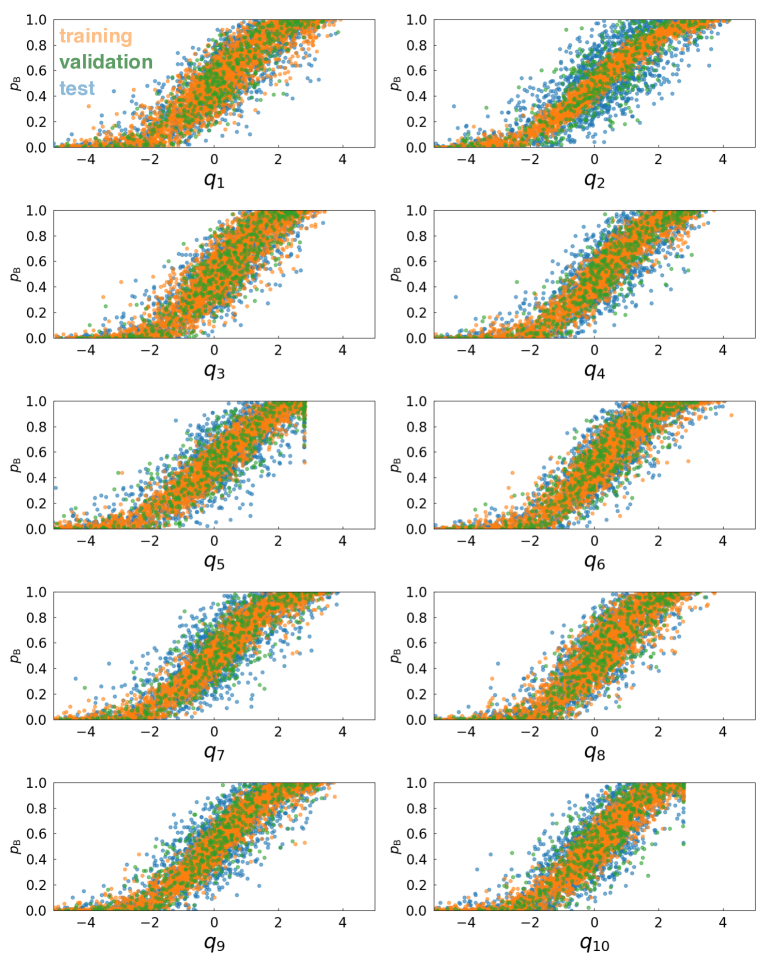
Figure S4: Scatter plots of the optimized coordinates ($q_{1}$ to $q_{10}$) and committors ($p_{B}$) in water. Orange, green, and blue in (a) and (b) denote the results from the training, validation, and test data sets, respectively.

The change of $p_{B}$ along $q_{1}$ in water is summarized in Fig. 8. The results for other RCs are in Figs. S4 and S5. The distribution of $p_{B}$ (Fig. 8(a)) is broader than the case in vacuum but follows a sigmoidal curve as a function of $q_{1}$. The histogram of $p_{B}$ near the TS (Fig. 8(b)) shows a peak at $p_{B}$$\sim$0.5 with the width of the histograms broader than those in vacuum. The results for the other optimized coordinates in Fig. S4 are mostly consistent with $q_{1}$. We note that only in the case of $q_{2}$, the histogram for the training data is sharply peaked while that for the test data is broad, implying that overfitting to the training data has occurred. This is consistent with the loss function values and RMSE results (Figs. 4(b) and 5(b), respectively).

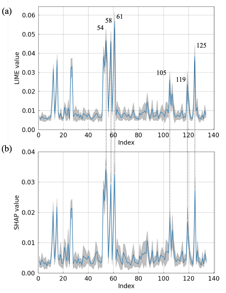
Figure S6: Contributions of CVs to RCs in water excluding $q_{2}$ extracted using (a) LIME and (b) SHAP in absolute values. Blue lines and gray shades denote the average and variance calculated from the 9 RCs.

Fig. 9 shows the contributions of CVs to the RCs at about the TS extracted by LIME and SHAP. Note that these analyses include $q_{2}$, because excluding $q_{2}$ only slightly changed the result (Fig. S6). Similarly to the case in vacuum, CV₆₁, CV₅₈, and CV₅₄, corresponding to $\phi$, $\phi$, and $\theta$, respectively, are found to be the three major CVs. Apart from these three CVs, CV₁₂₅, the electrostatic potential from the water on H₁₈ (V_ele(H₁₈)) (Fig. 1), shows up as a key feature from the solvent. In addition, CV₁₀₅ and CV₁₁₉, which are the electrostatic potential on H₈ and C₁₅, respectively, show notable contribution to the RC. Same trend is found in the SHAP result though the relative balance is somewhat changed. The scatter plots of V_ele(H₁₈) and $\phi$ or $\theta$, given in Figs. 10(a) and (b), respectively, do not show a clear correlation between the changes of CVs and $p_{B}$ or any apparent separatrix. On the other hand, the plot as a function of the three variables (Fig. 10(c)) shows that there is a weak correlation between V_ele(H₁₈) and $p_{B}$ near the separatrix in the ($\phi$, $\theta$) space. Thus the solvation coordinate V_ele(H₁₈) is contributing to the RC in a nontrivial manner. Interestingly, the importance of solvent effect to H₁₈ have also been indicated by Ma and DinnerMa and Dinner (2005) for the C_7eq $\leftrightharpoons$ $\alpha_{\mathrm{R}}$ transition through the torque coordinate as mentioned above.

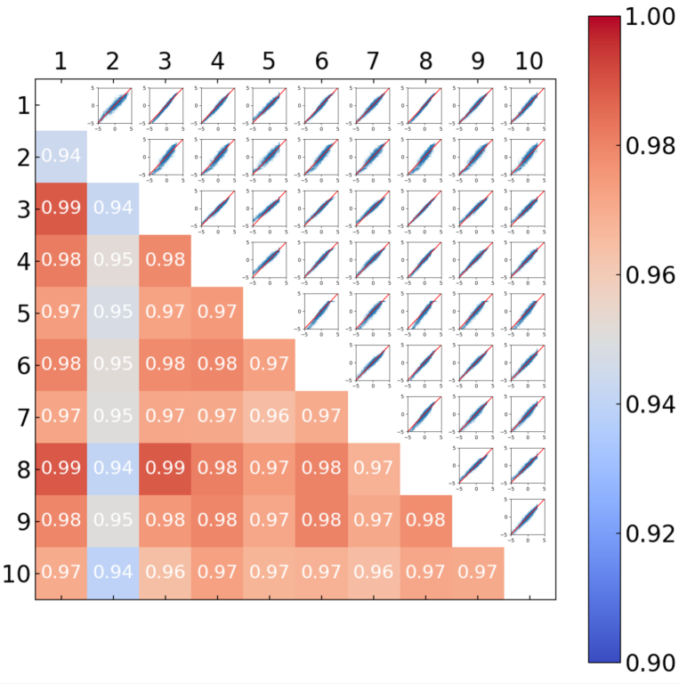
Figure S7: Scatter plots (top-right) and correlation coefficient (bottom-left) showing the correlation between the RCs from different optimized DNN models in water. $q_{i}$ denote the optimized coordinate from the $i$-th DNN model. Note that all data points are included in these plots.

Finally, the RCs in water are directly compared in Fig. S7. Compared to the vacuum results (Fig. S3), the deviation from the diagonal line is slightly larger even at $q_{i}\sim 0$ (i.e., near TS). Nevertheless, the overall correlation between the RCs are very high and found to be above 0.96 except for $q_{2}$. Furthermore, the correlation between $q_{2}$, which was indicated to be slightly overfitted, and other CVs is still above 0.94.

Thus, the current hyperparameter optimization framework successfully obtained the RC for the alanine dipeptide isomerization in water, where the DNN models can differ but the important features remain very similar.

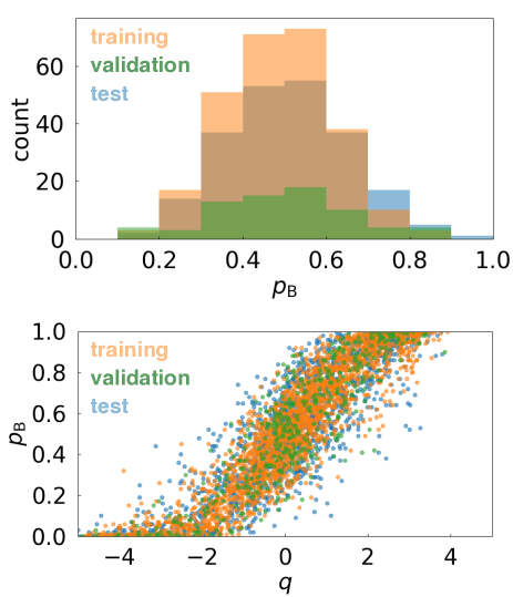
Figure 8: (a) Scatter plots of the optimized coordinate ($q$) and committor ($p_{B}$) for $q_{1}$ in water. (b) Distribution of $p_{B}$ for the points within $-0.2<q_{1}<0.2$. Orange, green, and blue in (a) and (b) denote the results from the training, validation, and test data sets, respectively.

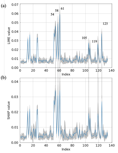
Figure 9: Contributions of CVs to the RCs in water extracted using (a) LIME and (b) SHAP in absolute values. Blue lines and gray shades denote the average and variance calculated from the 10 RCs.

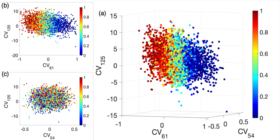
Figure 10: Correlations between the changes in CVs and $p_{B}$ in water from the scatter plots in the spaces of (a) CV₆₁ ($\phi$) and CV₁₂₅ (V_ele(H₁₈)), (b) CV₅₆ ($\theta$) and CV₁₂₅, and (c) CV₆₁, CV₅₆, and CV₁₂₅. Color range denotes the calculated $p_{B}$ at each point.

IV Summary

Machine learning approaches have become a popular tool in extracting the RCs for the reactions from many CV candidates in complex environments. DNN is especially powerful for obtaining the RCs with non-linear character, and XAI tool serves an complement to DNN by extracting the important feature from the complex DNN models and understanding the mechanism. Yet, the DNN model structure, defined by the hyperparameters such as number of layers and nodes per layer, can be highly flexible, and choosing the appropriate models has been a non-trivial and tedious task. To this end, we developed the hyperparameter tuning approach by introducing the Bayesian optimization method to determine the DNN models for RC optimization in an automatic manner. The DNN model was optimized so as to obtain a RC that can predict the changes of committors from the reactant to product in a smooth manner with a peak of $p_{B}$ $\sim$ 0.5 at the transition state ($q\sim$ 0).

The current approach was first applied to analyze the isomerization reaction of alanine dipeptide in vacuum. The RC was successfully obtained from 10 different initial conditions, where the RMSE of $p_{B}$ between the prediction from the RC and the actual data was about 0.005. The correlations betweent the 10 RCs were also very high ($>$0.99). On the other hand, the structure of the optimized DNN model, i.e., the hyperparameters, varied notably between the RCs. By applying the LIME and SHAP methods, all RCs wre found to have the same key features, i.e., $\phi$ and $\theta$. Thus, despite the apparent differences in the DNN models, all RCs share common physical mechanism for the reaction in vacuum with similar accuracy.

The hyperparameter optimization method was further applied to the isomerization reaction in water. The RC for the reaction in solution was successfully obtained in most cases (9 out of 10) where the RMSEs between the predicted and calculated $p_{B}$ for the test data were about 0.02. In one case ($q_{2}$) we found slight sign of overfitting, where the committor probability distribution and RMSEs for training and test data sets showed some discrepancy. Similarly to the case in vacuum, the hyperparameters were found to vary notably, but the successfully optimized RCs showed similar $p_{B}$-predictability and high correlation ($>$ 0.96). By analyzing the RCs using XML methods, every RC was found to have common key features, i.e., $\phi$, $\theta$, and the electrostatic potential from the water on H₁₈. We note that this solvent contribution to the hydrogen was also found in the torque coordinate proposed previously for a slightly different reaction pathMa and Dinner (2005), and the current DNN model was able to describe this from a rather simple set of CV candidates.

The current hyperparameter tuning framework can be applied to explore the RC for reactions in different systems straighforwardly. It is noted that here the RCs were optimized using slightly different data set, i.e., the same data was partitioned into slightly different training, validation, and test groups due to different random seed. Even when the same data set was used, the optimization converged to different optimal when different initial hyperparameters were used (not shown). Thus, the hyperparameter space of the current DNN model for RC is likely multimodal, and optimization of the hyperparamters gives similarly accurate RC but different DNN models depending on initial conditions. However, as the XAI analysis applied to these DNN models shows common key features, the current study indicates that suitably optimized DNN models can still obtain the same reaction mechanism despite the apparent difference in the model structure.

AUTHOR DECLARATIONS

Conflict of Interest

The authors have no conflicts to disclose.

Data availability

The data that support the findings of this study are available from the corresponding author upon reasonable request.

Supplementary Material

Investigating the hyperparameter space of deep neural network models for reaction coordinate optimization: Application to alanine dipeptide in water

Kyohei Kawashima¹, Takumi Sato², Kei-ichi Okazaki^3,4,a), Kang Kim^5,b), Nobuyuki Matubayasi^5,c), and Toshifumi Mori^1,2,d)

¹⁾Institute for Materials Chemistry and Engineering, Kyushu University, Kasuga, Fukuoka 816-8580, Japan
²⁾Department of Interdisciplinary Engineering Sciences, Interdisciplinary Graduate School of Engineering Sciences, Kyushu University, Kasuga, Fukuoka 816-8580, Japan
³⁾Research Center for Computational Science, Institute for Molecular Science, Okazaki, Aichi 444-8585, Japan
⁴⁾Graduate Institute for Advanced Studies, SOKENDAI, Okazaki, Aichi 444-8585, Japan
⁵⁾Division of Chemical Engineering, Department of Materials Engineering Science, Graduate School of Engineering Science, Osaka University, Toyonaka, Osaka 560-8531, Japan

^a)Electronic mail: keokazaki@ims.ac.jp
^b)Electronic mail: kk@cheng.es.osaka-u.ac.jp
^c)Electronic mail: nobuyuki@cheng.es.osaka-u.ac.jp
^d)Electronic mail: toshi_mori@cm.kyushu-u.ac.jp

Table S1: Definitions of collective variables used for the reactions in vacuum and water.

dihedrals (CV 1-45: cosine, 46-90: sine)
index	atom number
$01-03$	1 - 2 - 5 - 6	1 - 2 - 5 - 7	3 - 2 - 5 - 6
$04-06$	3 - 2 - 5 - 7	4 - 2 - 5 - 6	4 - 2 - 5 - 7
$07-09$	2 - 5 - 7 - 8	2 - 5 - 7 - 9	6 - 5 - 7 - 8
$10-12$	6 - 5 - 7 - 9	5 - 7 - 9 - 10	5 - 7 - 9 - 11
$13-15$	5 - 7 - 9 - 15	8 - 7 - 9 - 10	8 - 7 - 9 - 11
$16-18$	8 - 7 - 9 - 15	7 - 9 - 11 - 12	7 - 9 - 11 - 13
$19-21$	7 - 9 - 11 - 14	10 - 9 - 11 - 12	10 - 9 - 11 - 13
$22-24$	10 - 9 - 11 - 14	15 - 9 - 11 - 12	15 - 9 - 11 - 13
$25-27$	15 - 9 - 11 - 14	7 - 9 - 15 - 16	7 - 9 - 15 - 17
$28-30$	10 - 9 - 15 - 16	10 - 9 - 15 - 17	11 - 9 - 15 - 16
$31-33$	11 - 9 - 15 - 17	9 - 15 - 17 - 18	9 - 15 - 17 - 19
$34-36$	16 - 15 - 17 - 18	16 - 15 - 17 - 19	15 - 17 - 19 - 20
$37-39$	15 - 17 - 19 - 21	15 - 17 - 19 - 22	18 - 17 - 19 - 20
$40-42$	18 - 17 - 19 - 21	18 - 17 - 19 - 22	2 - 7 - 5 - 6
$43-45$	5 - 9 - 7 - 8	9 - 17 - 15 - 16	15 - 19 - 17 - 18
electrostatic (Vele) & van der Waals (VvdW) potentials
index	atom number
$91-93$	V${}_{\mathrm{ele}}(1)$	V${}_{\mathrm{vdW}}(1)$	V${}_{\mathrm{ele}}(2)$
$94-96$	V${}_{\mathrm{vdW}}(2)$	V${}_{\mathrm{ele}}(3)$	V${}_{\mathrm{vdW}}(3)$
$97-99$	V${}_{\mathrm{ele}}(4)$	V${}_{\mathrm{vdW}}(4)$	V${}_{\mathrm{ele}}(5)$
$100-102$	V${}_{\mathrm{vdW}}(5)$	V${}_{\mathrm{ele}}(6)$	V${}_{\mathrm{vdW}}(6)$
$103-105$	V${}_{\mathrm{ele}}(7)$	V${}_{\mathrm{vdW}}(7)$	V${}_{\mathrm{ele}}(8)$
$106-108$	V${}_{\mathrm{vdW}}(8)$	V${}_{\mathrm{ele}}(9)$	V${}_{\mathrm{vdW}}(9)$
$109-111$	V${}_{\mathrm{ele}}(10)$	V${}_{\mathrm{vdW}}(10)$	V${}_{\mathrm{ele}}(11)$
$112-114$	V${}_{\mathrm{vdW}}(11)$	V${}_{\mathrm{ele}}(12)$	V${}_{\mathrm{vdW}}(12)$
$115-117$	V${}_{\mathrm{ele}}(13)$	V${}_{\mathrm{vdW}}(13)$	V${}_{\mathrm{ele}}(14)$
$118-120$	V${}_{\mathrm{vdW}}(14)$	V${}_{\mathrm{ele}}(15)$	V${}_{\mathrm{vdW}}(15)$
$121-123$	V${}_{\mathrm{ele}}(16)$	V${}_{\mathrm{vdW}}(16)$	V${}_{\mathrm{ele}}(17)$
$124-126$	V${}_{\mathrm{vdW}}(17)$	V${}_{\mathrm{ele}}(18)$	V${}_{\mathrm{vdW}}(18)$
$127-129$	V${}_{\mathrm{ele}}(19)$	V${}_{\mathrm{vdW}}(19)$	V${}_{\mathrm{ele}}(20)$
$130-132$	V${}_{\mathrm{vdW}}(20)$	V${}_{\mathrm{ele}}(21)$	V${}_{\mathrm{vdW}}(21)$
$133-134$	V${}_{\mathrm{ele}}(22)$	V${}_{\mathrm{vdW}}(22)$

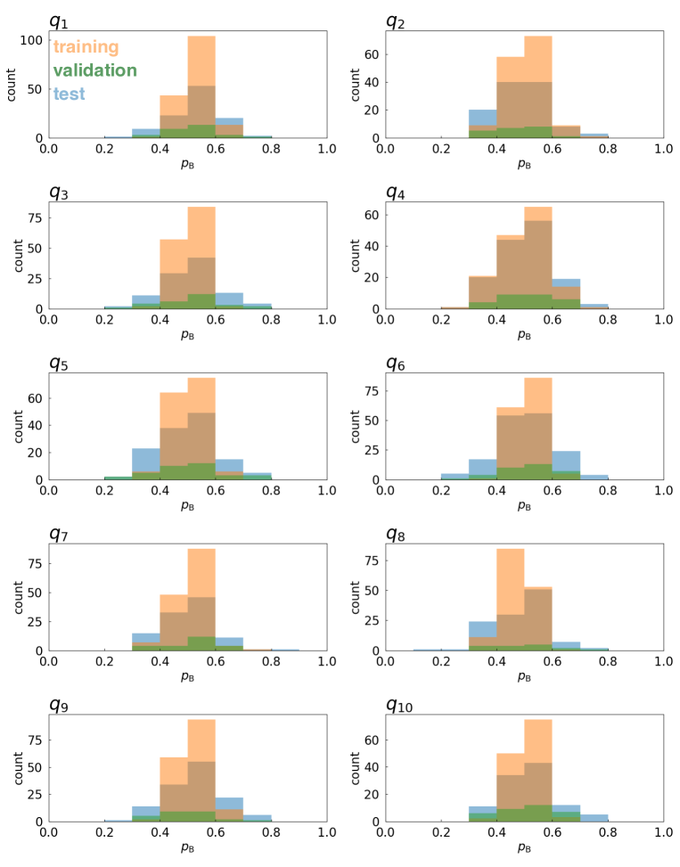
Figure S2: Histogram of the committors for the data points within $-0.2<q<0.2$ for $q_{1}$ to $q_{10}$ in vacuum. Orange, green, and blue in (a) and (b) denote the results from the training, validation, and test data sets, respectively.

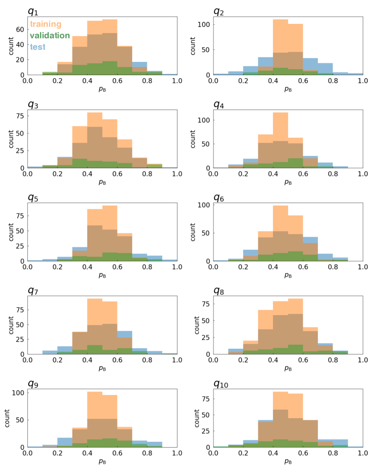
Figure S5: Histogram of the committors for the data points within $-0.2<q<0.2$ for $q_{1}$ to $q_{10}$ in water. Orange, green, and blue in (a) and (b) denote the results from the training, validation, and test data sets, respectively.