Exponential tail estimates for quantum lattice dynamics
Abstract.
We consider the quantum dynamics of a particle on a lattice for large times. Assuming translation invariance, and either discrete or continuous time parameter, the distribution of the ballistically scaled position converges weakly to a distribution that is compactly supported in velocity space, essentially the distribution of group velocity in the initial state. We show that the total probability of velocities strictly outside the support of the asymptotic measure goes to zero exponentially with , and we provide a simple method to estimate the exponential rate uniformly in the initial state. Near the boundary of the allowed region the rate function goes to zero like the power of the distance to the boundary. The method is illustrated in several examples.
1. Introduction
It is an almost universally accepted view that at very small scales the model of spacetime as a continuum must be modified. Yet, one of the most natural ways of implementing this idea, namely replacing the continuum by a lattice, has been plagued by the somewhat arbitrary breaking of isotropy involved in choosing the lattice axes. One thus needs to explain how at large scales an exactly circular light cone can govern the propagation in a cubic lattice, a case of inverse symmetry breaking [25]. Moreover, one would like to have an explicit bound on the fuzziness of the cone: The probability for “faster-than-light” signals will be non-zero in such a model, but these signals should be weak on a large scale, and decrease rapidly for speeds appreciably larger than the speed of light of the continuum model. In this paper we will provide a technique to get such bounds, namely large deviation type [10] estimates: The total probability for a quantum particle to be found outside the cone, say at any speed larger by than allowed, decreases exponentially in time which is sometimes called “evanescence” of the particle’s wave function in analogy to optical waves [5]. We provide a formula for the rate of exponential decrease as a function of . Typically, the total probability outside an -neighbourhood of the cone goes like .
Effective propagation cones have, of course, been noted before. In the context of quantum walks (discrete time unitary lattice dynamics) they appear in the asymptotic form of the position at large times , scaled as a velocity by considering [12, 2, 1]. As in the solid state context (continuous time Hamiltonian lattice dynamics), this scaled asymptotic position converges to the group velocity operator. The spectrum of this operator thus defines the propagation region, which is not necessarily a spherical cone and might not even be convex. Spherical propagation regions are often related to the appearance of “Dirac points”, certain singular points in the band structure of lattice systems such as graphene. However, the mere convergence of only allows for the conclusion that the total probability outside the cone goes to zero, not for how fast and not for how the rate depends on the distance from the cone.
Our technique for providing such bounds on the rate of convergence applies to both discrete time and continuous time Hamiltonian dynamics. We assume only translation invariance and that the number of states per unit cell is finite. It is closely related to stationary phase/steepest descent evaluation [9]. However, it seems more direct, especially if one does not want to estimate the probability amplitudes for individual points, but the total probability for large regions outside the cone.
Our paper is organized as follows: in the next section we describe the setting in which we are working and state the main estimate which is proved in Section 3. In Section 4 we discuss this estimate and the limit cases, and show several properties of the involved quantities. Emblematic examples are discussed in Section 5.
2. Main result
2.1. Setting and statement of the main estimate
We consider systems, whose configurational variable (for a single particle: the position) is confined to a point lattice in -dimensional Euclidean space. At each lattice site we allow some finite dimensional Hilbert space of internal states with . The overall system Hilbert space is thus . We typically write as a -valued square summable function on so that the -component of the position operator is the multiplication operator .
In such a system we consider a coherent quantum mechanical time evolution, either generated by a Hamiltonian (the continuous time case) or by a unitary operator in (the discrete time case). By we denote the evolution after time , i.e., in the continuous time case and the (integer) matrix power in the discrete time case. In either case we require that commutes with the lattice translations. Thus the dynamics is partially diagonalized by the Fourier transform
| (2.1) |
where , the Brillouin zone, which is to be considered with periodic boundary conditions, i.e., as the -torus. We equip with the normalized Haar measure , which makes unitary from to . By translation invariance, or become matrix valued multiplication operators, i.e.,
| (2.2) |
and similarly for . Since is -valued, is a unitary -matrix for every . For example, the “Hadamard walk”, a standard example of a one-dimensional quantum walk with , has
| (2.3) |
This is a nearest neighbour dynamics, because only and no higher powers appear. Generally, a walk has maximal jump length if each entry of is a trigonometric polynomial of absolute degree . Similar remarks apply to . We generalize this further by allowing to be an infinite series. Our standing “locality” assumption is then:
Assumption 1.
has an entire analytic extension from to .
Note that the analogous assumption on carries over to . The growth of in the imaginary direction is known to express decay properties of the evolution. For example, when has finite jump length , is of exponential type, i.e., satisfies a bound , which by the Paley-Wiener theorem implies that an initially localized state is strictly localized in a ball of radius . Of course, this is anyhow obvious from the meaning of the jump length, but it shows how the growth of the analytic extension relates to propagation. Our main result will refine this connection.
We are interested in the position distribution for large times. Since there is no dissipation, particles will generically spread ballistically, i.e., the scaled quantity is expected to have a limit distribution. For any measurable set we introduce the probability
| (2.4) |
for finding a value in a position measurement at time , starting from the initial state . Here denotes the indicator function of the set , so is the operator of multiplication by . It turns out that in the described setting the limit of (2.4) exists in the weak sense, and all the limit measures have their support in a compact, -independent set , which we call the propagation region in velocity space [12, 2]. A precise formulation will also be given in Sect. 2.2, together with an explicit formula for the limits and proofs.
Our main interest here is the behaviour of the probability measures outside of the propagation region. From the statements given, it is clear that when , we get for all . But how fast is this convergence? Our main theorem will establish that it is exponential, with a rate increasing with the distance between and , i.e.,
| (2.5) |
where is an exponential rate that is independent of the initial state. If is split into different regions , estimates of this type are dominated by the smaller rate, i.e., when , we have for large , and hence . In this sense only the points with the lowest rate “” contribute. We say that a lower semi-continuous function is a rate function for the process, if
| (2.6) |
for every which initially has compact support, and every closed set . We will work with the form (2.6), and regard (2.5) as a heuristic interpretation. Strictly speaking, this allows a sub-exponential time dependence of the constant, or else (2.5) is to be read as a bound for every with a time-independent constant .
Estimates of this type belong to the theory of Large Deviations [10]. Typically, in that theory one also shows lower bounds, but since these would be state dependent, we do not consider them here.
With these preparations our estimate can be stated as follows:
Theorem 2.1.
In the setting described above, a rate function in (2.6) can be taken as the Legendre transform
| (2.7) |
of a function that can be computed directly from , respectively , as
| (2.8) | ||||
| respectively | ||||
| (2.9) | ||||
where denotes the Brillouin zone.
2.2. Group velocity and propagation region
Here we provide short proofs of the general claims made about the limiting velocity distribution. These are known results [12, 2], so our main reason for presenting them here is to introduce the proof method, a variant of which will be central to the proof of Theorem 2.1. We begin by diagonalizing or for every :
| (2.10) | ||||
where the determine the eigenvalues ( is only defined in the discrete time case) and the are rank-1 eigenprojections. Obviously, we have to be careful about degeneracies. Unlike in the one-dimensional () case, the analyticity of does not imply that we can also choose the branch functions analytic, not even locally. On the other hand, analyticity near is easy to see for any nondegenerate branch : In that case we can set up a Cauchy Resolvent Integral formula around the isolated point in the complex plane providing analytic expressions for both and . The same holds for isolated branches with higher multiplicity, which arise by tensoring with an additional internal space , on which acts like the identity. Points for which such an analytic choice is possible are called regular in the theory of analytic matrix functions [4, § S3]. It is shown there that the regular points form a connected open submanifold, so the irregular/singular points are of Lebesgue measure zero. Thus the expressions (2.10) make sense almost everywhere, including small open neighbourhoods. Even degenerate points may be regular, where two bands just form intersecting analytic manifolds. The prototype of a singular point is the tip of a cone, as for example in , where and are Pauli matrices. Even when there are no singular points, the bands may wrap around the torus in a non-trivial way. That is, following a band along a closed, but not contractible path one may end up in another branch.
With this information we can introduce the group velocity operator. This operator also commutes with translations so that it acts by multiplication with a -dependent matrix. It is the vector operator whose -coordinate is defined (at every regular point) as
| (2.11) |
An alternative definition, which does not require diagonalization, but obviously coincides with the above at every regular point is
| (2.12) |
and, for the discrete time case,
| (2.13) |
where the are now the non-degenerate projections of the functional calculus belonging to the distinct eigenvalues. The key feature is that the components of commute with or and almost everywhere with each other. That is, as matrix-valued multiplication operators on , the do commute and hence have a joint functional calculus, so we can evaluate bounded measurable functions on , getting an operator . The spectral projection for is then , and the joint spectrum is the complement of the largest open set such that . Since is assumed to be analytic and is compact, is also bounded, and hence is compact. We can construct almost-eigenvectors of for eigenvalue tuple at every regular point, so we have that at every regular point, and since acts almost everywhere by multiplication with such numbers we have
| (2.14) |
The reason to study these objects, and the justification for calling the propagation region, is given in the following Proposition. It is basically well-known, and the reason for calling the group velocity operator. In the walk context the first statement (apart from worked individual examples) seems to be [12]. The technique there is based on the convergence of moments, which is slightly problematic, because the moments might fail to exist for the initial state and all through the evolution. We give here a proof based on characteristic functions, which appeared in [2] in a much more complex context, which perhaps obscured the structure of the argument. However, it is this basic idea that will be needed later for the proof of Theorem 2.1.
Proposition 2.2.
For every density operator , the probability measure defined in (2.4) converges weakly to the distribution of in . Explicitly:
| (2.15) |
for every continuous function vanishing at infinity, with evaluated on both sides in the respective functional calculus.
Proof.
The weak convergence is equivalent by the continuity theorem for characteristic functions [17] (aka. Levy’s convergence theorem [18][19, Théorème 17]) to the pointwise convergence of characteristic functions, i.e., to the special case of (2.15) for for all . We fix one such now.
Exponentials of are shift operators in the momentum representation. To utilize this, we introduce the operators
| (2.16) |
This is an operator that once again commutes with translations. So in the momentum representation on it acts as a matrix multiplication operator, namely
| (2.17) |
With the same transformation for we get
| (2.18) |
where the second equality is for the continuous time case, with , and , which multiplies in momentum representation with . It is worth noting that while the operators on the whole space are unitarily conjugate to each other by virtue of (2.16), the matrix is not conjugate to and generally these have different spectrum.
We now claim (in either case) the strong limit formula
| (2.19) |
For the proof of this claim note first that all operators involved are unitary, so strong convergence is equivalent to weak convergence, i.e., we only have to show the convergence of all matrix elements. Moreover, all operators in (2.19) commute with translations, and hence act by multiplication with uniformly bounded matrices in momentum space. By the Dominated Convergence Theorem it therefore suffices to show that
| (2.20) |
We may therefore assume that is a regular point, and that in the neighbourhood of the eigenprojections and eigenvalues are analytic functions. By (2.10) the left hand side is hence
| (2.21) |
Each of the finitely many terms with goes to zero, because as , and these operators are multiplied by a bounded function. For the diagonal terms the exponent converges to a directional derivative as :
| (2.22) |
Comparing with (2.11), this is precisely the exponent of the corresponding term in which proves (2.19).
Now consider an arbitrary pure state density operator . Then the characteristic function of its scaled position at time is
| (2.23) |
According to the claim just proved the first vector goes in norm to and the second goes to by strong continuity of the one-parameter group generated by . This proves the proposition for pure states. For mixed states one can use a trace norm approximation by a linear combination of pure states. ∎
3. Proof of Theorem 2.1
We consider now the same basic technique as in the proof of Proposition 2.2, replacing, however, by for . Schematically replacing by in (2.16) and (2.17) we get
| (3.1) | ||||
| and | ||||
| (3.2) | ||||
but we still have to make rigorous sense of these identites. In (3.2) the right hand side contains the analytically continued , which exists by Assumption 1. Hence can and will be defined by this formula. The -dependent matrix it multiplies with is continuous, and since is compact, is uniformly norm bounded for . Hence is a bounded operator, and the family for is a norm analytic family of bounded operators. However, to make good use of this analytic extension we also need to give an interpretation of the operator product in (3.1). This is done in the following Lemma.
Lemma 3.1.
Let and denote by the intersection of the domains of the selfadjoint operators with . Then, for we have , and for
| (3.3) |
Proof.
For , the function can be differentiated in norm for , and has continuous boundary values on this “strip”. Consider now a vector , which is compactly supported in position, so that, in particular, . Then consider the equation for complex :
| (3.4) |
This holds for by (2.16). Hence it can be extended to all for which both sides are analytic. The vector is everywhere anti-analytic, so the left hand side is entire. For the right hand side, we just established that the vector is analytic in the strip , and is an entire analytic family by assumption. The equality furthermore extends to the boundary values, in particular to any with and . Thus, for in a core of the selfadjoint operator we have that . Hence , and . ∎
The core of the proof of Theorem 2.1 is the following exponential estimate for the expectation of :
Lemma 3.2.
Let be a density operator and such that for with . Then, for such ,
| (3.5) |
where is the function given in Theorem 2.1.
Note that here we need a condition on the initial distribution, whereas in Propopsition 2.2 this is missing: The initial distribution is absorbed by the ballistic scaling. The condition is, of course, satisfied for any strictly localized state, but one can also find states, say, with power law decay, for which the expectation under the limit is constant equal to .
Proof.
Note first that the condition is only about the initial distribution of . In this condition is taken as always defined, but possibly infinite, by integrating the -expectation of the spectral measure of against the exponential function. We argue first, that it suffices to prove the Lemma for pure states . Indeed, if the assumption holds for it also holds for every convex component of , i.e., every vector such that with . Furthermore, if the bound holds for some ’s it also holds for finite sums , where we can ignore normalization factors, which are scaled away on the left hand side with . Moreover, we can transfer to a norm convergent sum , because is the supremum of the corresponding expressions using the partial sums , and on the right hand side is independent of . Hence the spectral resolution of reduces the proof to the pure state case.
For , the premise is just with defined as in Lemma 3.1. That Lemma was stated in such a way that its condition propagates with , i.e., it implies (by induction) also that , and . But then we find
| (3.6) |
Hence taking the logarithm and dividing by , we get that
| (3.7) |
In fact, on the right hand side the limit (not just the limit superior) exists, because is a subadditive function. For discrete time, is defined as the spectral radius of , so in (3.7) we get twice the logarithm of the spectral radius of . In continuous time, the limit along can similarly be evaluated, and by the spectral mapping theorem gives . The same holds along for any , so this is the limit. In either case, the operators involved are matrix multiplication operators, so the spectrum is the closure of the union over of the spectra of , and similarly for . This spectral supremum is the function given in Theorem 2.1. ∎
Our next task is to turn this into an estimate of probabilities of sets . We begin with half spaces
| (3.8) |
for some constants and . Then, for all , the indicator function of is everywhere . Therefore, by the functional calculus for the self-adjoint operator ,
| (3.9) |
and with (2.4):
Combining with (3.5), we can summarize this as
| (3.10) |
Our task in the remainder of the proof will be to extend this from half spaces to more general sets, for which we largely follow the proof of [10, Lemma VII.4.1.]. Throughout we will fix some , to be thought of as a reference rate, and ask for which sets the probability decreases at least with rate , i.e., . The largest half spaces for which (3.10) guarantees such decrease are
| (3.11) |
where we suppress the dependence on the fixed in the notation. It will be convenient to consider also the open half space , and their complements .
The first extension is to sets which are contained in a finite union of open half spaces,
| (3.12) |
Indeed, in this case
and hence
| (3.13) |
Let us denote by the union of all open half spaces (for fixed ). Its complement is the level set defined as
| (3.14) |
of the rate function defined by (2.7). We claim that for every closed set we can find a finite collection of satisfying (3.12). This is evident for compact , because we may choose a finite subcover of the cover .
For general closed we follow a construction of [10, Lemma VII.4.1] exploiting that in a union of half spaces infinity is anyhow well covered. More formally, let be an open ball containing , and denote its closure and boundary by and (see Figure 1). Consider the set
| (3.15) |
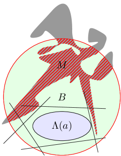
This is compact as the union of two compact sets, so we can find finitely many with . The complement is a finite intersection of half spaces, i.e., a polytope. Since is in the complement of , is entirely contained in . Hence , and since , we have also found the desired covering (3.12). To conclude: (3.13) holds for every closed subset .
To conclude the proof of Theorem 2.1, let be an arbitrary closed set and . As we argue in the next section, is lower semi-continuous with compact level sets and hence this infimum is actually attained on . Since for the bound in (2.6) is trivial, we assume . Consider any , which for just means any positive number. The level set is disjoint from , and so . By the previous paragraph this implies (3.13). Since was arbitrary we finally get the bound (2.6).
4. Discussion of the bound and general properties
4.1. Elementary properties
(1)
Obviously, by (2.8) and (2.9), . Hence we can put in (2.7) to get . The rate function can be infinite, which indicates superexponential decay. A good example is given also in Section 4.2, where in some velocity region the probability vanishes exactly, and .
(2) is convex and lower semicontinuous
Convexity and lower semicontinuity are clear for any Legendre transform, and more generally for any pointwise supremum of continuous affine functions.
(3) for , the closed convex hull of the propagation region.
Indeed, if we have a set such that for some and large , the left hand side of (2.6) has a lower bound , which goes to zero, implying . Since is lower semicontinuous, this implies that vanishes on . Since the rate function is convex, its level sets and in particular the zero set is also convex, so contains . The propagation region may well fail to be convex, in which case there is a region for which our bound has no exponential rate prediction, although the probability does go to zero. An example is provided in Section 5.3 below.
(4) is continuous
Consider the function , where ‘’ denotes the spectral radius. By our standing assumption, is entire analytic, so jointly continuous. Moreover, the spectral radius in a fixed finite matrix dimension is continuous, because the coefficients of the characteristic polynomial are, and the zeros of a polynomial are continuous functions of the coefficients (a standard result; see e.g., [13]). The continuity of thus follows from the purely topological Lemma that for any jointly continuous function with compact, the partial supremum is continuous [26]. For completeness, we provide the lemma in Appendix A.
(5) has compact lower level sets
The lower level sets
| (4.1) |
defined in (3) are closed for all because is lower semicontinuous. To show their boundedness we only need one consequence of the continuity of , namely that is bounded on any sphere of sufficiently small radius . Suppose for . Then, for , we have for all , and hence for . Hence is contained in a ball of radius .
4.2. Large and relation to trivial propagation bounds
Consider first the walk case, i.e., the discrete time evolution with strictly finite jumps, characterized by , where is the finite set of possible jumps.
Lemma 4.1.
We have for all outside the convex hull of the possible jumps .
Proof.
The continuous time analogue of the last bound is somewhat similar to Lieb-Robinson bounds in statistical mechanics [16, 21, 20]: One needs only rough information about the size of the Hamiltonian terms to get propagation in a cone (up to exponential tails). We describe one simple version. To state it, we assume without loss that the origin lies in the interior of with , where . (If this is not the case, add at the origin.) The so-called “gauge functional” of this set is
| (4.3) |
This is like a norm, but with a “unit ball” which need not be symmetric around . Then
Lemma 4.2.
With ,
| (4.4) |
Note that this bound is non-trivial only for , but then grows a bit faster than linearly. Moreover, it sets a bound on the propagation region, namely
| (4.5) |
Proof.
Let be a complex eigenvalue of , and a corresponding normalized eigenvector. Then
which we can summarize as
| (4.6) |
where is defined as in the proof of Lem. 4.1. Now suppose that , i.e., . Then there is some such that , but . We will get a lower bound on , by extending the supremum (2.7) only over subset of , where . Thus
where we have assumed that , since otherwise the supremum is attained at , giving the trivial bound . Since this bound is monotone in , we may replace by , which yields (4.4). ∎
4.3. Small and behavior near
In order to analyze the behavior of the rate function near the boundary of the propagation region , we consider the behavior of for small . We first note that as a consequence of the identity , any isolated eigenvalue satisfies
| (4.7) |
Therefore, around any regular point the even powers in the expansion of this expression vanish, and we can write:
| (4.8) |
To obtain an expression for , according to (2.8) we have to take the maximum of this with respect to . Doing this in the approximation (4.8) by (2.14) directly leads to , with defined as above by . The corresponding rate function vanishes on , as does, but is infinite everywhere outside . The approximation (4.8) is thus useless for learning anything about the behavior of near the boundary .
We will thus go to higher orders in the Taylor expansion (4.8). However, it is clear from the outset that such an expansion cannot lead to a full evaluation of in general: This is defined as the global supremum of a function that is periodic in , and the expansion will destroy that property and introduce artifacts, especially in the polynomial growth for large . Similarly, the Legendre transform to the rate function can only be estimated from below from any local description of . Therefore, the best we can hope for is a heuristic description of the typical behaviour near the boundary.
So let us fix and start from the maximization of (4.8) with respect to and . This is the same as the maximization of for the dual direction , i.e., exactly the same variational problem we need for determining the boundary points of . We assume a unique solution, as will be generically the case, and accordingly fix and in the sequel. will be the base point for the Taylor expansion of . We note that these data are generally different for and for . The expansion then reads
| (4.9) | ||||
Here we use the shorthand and the summation convention by which repeated greek indices are understood to be summed over. The combinatorial factors arise from a in the Taylor expansion and the observation that the derivatives are permutation symmetric in the indices, so terms with the same number of - and -components but in different positions are equal. Moreover, the term with second derivatives of is left out preemptively: It vanishes because vanishes at the extremum. For the same reason, in the third order term the matrix is negative semidefinite.
In order to evaluate via (2.8) we need to compute the maximum of this expression over . For the dominant contribution, the term in the second line of (4.9), this is easy: By choice of its maximum is at . We expect a small correction to this when higher order terms are included. Setting the derivative of the right hand side of (4.9) to zero leaves leaves the linear term from the second line and, from the third, a constant term plus a term , which we neglect. Assuming the matrix to be invertible, we can solve for and get a correction . Inserting that back into the right hand side we get a correction , which is neglected in comparison to the higher order terms that we left out in the first place. Thus we conclude that to order we can set .
Let us introduce a variant of the function , a “boundary version”, in which only this conclusion is realized, i.e. , where are chosen to maximize . Then we can summarize the above heuristic discussion as
| (4.10) |
We will use this for computing the Legendre transform for half-ray by half-ray, i.e., along sets , for some unit vector . Then with , and due to the negative definiteness of . Thus we need
Lemma 4.3.
Let , , and be such that
Consider its Legendre transform . Then for :
| (4.11) |
Proof.
For we have to maximize a function of the form , which has a unique maximum for at , where its value is the first term on the right hand side of (4.11). To estimate the error term, set with for . Then for we have , so the bound on applies at , and
∎
Note that when we just assume to be known asymptotically for we cannot do better, since the true maximum could be attained anywhere on the half axis. However, if we add the assumption that is strictly convex, the local maximum in the proof must be the unique maximum, and we get an asymptotic equality as .
Let us summarize the heuristic estimate for the boundary behaviour of the rate function . Every boundary point will contribute a lower bound. More precisely, each such bound is associated with a normal direction and a boundary point , with chosen to maximize . We now assume that (4.10) holds and apply Lemma 4.3. The argument in the Lemma will be , , and
| (4.12) |
Then
| (4.13) |
Here denotes the positive part of , and we use this to express that the bound is non-trivial only for the points with , for which surely . For the overall bound one can take the supremum over all .
5. Examples
5.1. 1D Qubit walk
The asymptotics of quantum walks has been mostly investigated in the allowed region: in the one-dimensional setting [15, 7], in the two-dimensional setting [24, 3] and in arbitrary dimension [12, 2]. To our best knowledge, only two studies [8, 23] have been made of the asymptotics outside of the propagation region. In these studies a detailed stationary phase analysis was carried out involving the choice of contours in the complex plane. In addition to the exponential decay (2.6), this also gives the prefactors. Hence our method provides less information, but is much simpler to apply, and therefore has a better chance to analyze more complex cases. The simplest walks are of the form
| (5.1) |
with . Since , the dispersion relations are entirely determined by . The phase of can be compensated by a shift in , which is irrelevant for our question, so we assume from now on that . Then has the eigenvalues . This gives the group velocities
| (5.2) |
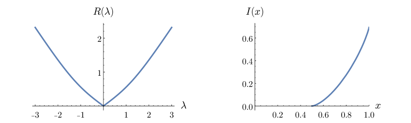
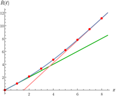
which takes their extrema for . So these are the boundary points of the propagation region. The maximum of for is also assumed at . Indeed, the derivative of this expression with respect to equals zero iff , which, after some algebra, yields the -independent equivalent condition . Hence in this case we have with as in (4.10). With this information we directly get from (2.9):
| (5.3) |
It turns out that the equation can be solved explicitly for , which gives
| (5.4) |
for , and in this range the Legendre transform
| (5.5) |
These functions are displayed in Fig. 2. This coincides with [23, (1.17)], but disagrees with [8].
5.2. A 2D walk with circular light cone
In a one-dimensional system the branches can always be chosen locally to be analytic. In fact, a basic result of perturbation theory [14, §1. Theorem 1.10] states that even at degenerate points one can make this choice. In higher dimensions one aspect of this structure survives: along any straight line through a degenerate point , say , one can pick analytic branches, and in particular some discrete set of slopes . However, these slopes in general do not belong to several intersecting analytic functions (in first order an intersection of planes) but may instead form a cone. The example we give here is perhaps the simplest in which this happens. Moreover, the conical singularity is essential for determining the outer boundary of the propagation region , which in this case is a disc. We set
| (5.6) |
which is equivalent to the product of two one-dimensional walks of the form (5.1) for . Its dispersion relation is
| (5.7) |
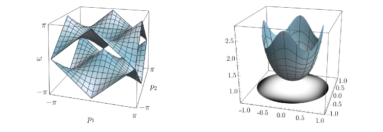
The conical structure at becomes apparent when we expand in a Taylor series in :
| (5.8) |
where . Of course, the same phenomenon happens at all points where , i.e., . This qualitatively explains Figure 3. The group velocity can be determined directly from (5.6):
| (5.9) |
with modulus
| (5.10) |
This is a monotone function of each , and equal to , whenever one of these variables is equal to one. Hence the propagation region is contained in the disc . The boundary points are all attained, but apart from the points on the axes only in the limit (compare (5.8)). The velocity distribution starting from the origin (i.e., with flat momentum distribution is shown in Figure 3.
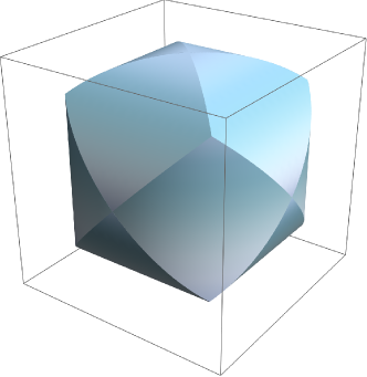
5.3. A 2D walk with non-convex propagation region
There is no reason why the propagation region should be a convex set. Figure 4 provides a somewhat minimal example. It is in the Hamiltonian context, without internal degree of freedom () and the Hamiltonian
| (5.11) |
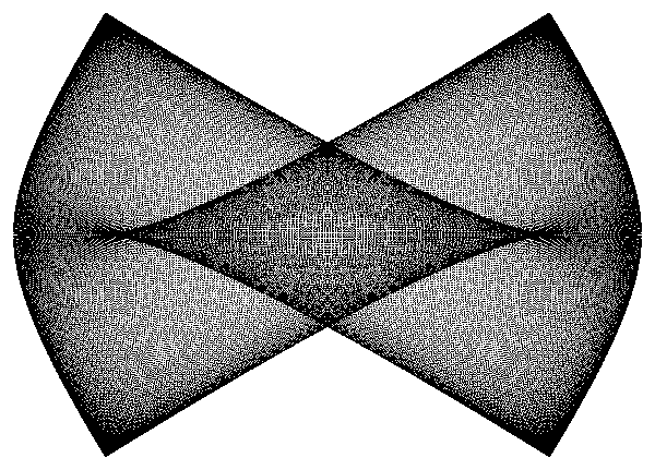
For an example in the walk context, see [3, Figure 3].
Of course, it is to be expected that large deviation bounds depending on the distance from the boundary also hold inside the non-convex indentations. However, our methods do not provide such statements. They give a positive rate function only outside the convex hull of (recall that we approximate by half spaces).
5.4. 3D cones and rate functions
Some quantum walks on the three-dimensional cubic lattice were proposed by Bialinycki-Birula [6] as discrete approximations to the Weyl, Dirac, and Maxwell equations. The interest in that paper is mainly in the continuum limit, and the possible variations of nearest neighbour walks automata for which this works. But one can take the discrete model as a system in its own right and analyze its propagation properties. Let us consider the simplest of these, the “Weyl equation” model in [6]. We then have , and
| (5.12) |
This gives
| (5.13) |
A characteristic feature here are conical singularities at and eight inequivalent points in the Brillouin zone, where , meaning that all and each matrix factor in (5.12) is . Expanding the cosine of (5.13) to second order in a small deviation from such a conical point , we get, for any combination of the signs ,
| (5.14) |
This is in keeping with the remarks in Section 2.2 on regular vs. singular points in a dispersion relation. Along a straight line through we can use one-parameter perturbation theory, in which we can always choose analytic branches, corresponding to the straight lines in the boundary of the cone, but as a function of three parameters is not analytic. In the limit taken in [6] only small momenta survive, so the propagation is indeed exactly the familiar light cone from relativistic physics. However, in this model faster propagation speeds can arise from points at a finite distance from the singularities. The overall propagation region is shown in Figure 5.
To get a spherical propagation region, we consider a modified model, on the same lattice and also with , and with exactly the same conical points , namely
| (5.15) | ||||
| (5.16) |
The modulus of the group velocity is then given by
| (5.17) |
where, in the second line we have abbreviated . Since the fraction in the second line is manifestly positive, we get . The maximum is reached at the conical points , where .
In order to compute the rate function we first notice that the analytic continuation of to complex is still a -matrix with determinant , so the trace (equal to ) determines the secular equation and hence both eigenvalues. That is, all information we need to evaluate from (2.9) is contained in the analytic continuation of (5.16).
We further reduce the problem by not looking at the full rate function, but a radial version of it: retains some of the lattice symmetry and is certainly not a rotation invariant function. As described in the introduction, we are however, mainly interested in an upper bound on the probability leakage outside a ball with slightly superluminal speed. We therefore look for a “radial rate function” such that if . Then the bound (2.6) for the probability outside a ball of radius becomes
| (5.18) |
which vanishes up to . The Legendre transform is friendly to the radial reduction: Suppose that , whenever . Then, for ,
| (5.19) |
which is the Legendre transform of . Here the inequality signs were chosen to make and automatically monotone.
This leaves us with the task to compute, for every the dual radial rate function
| (5.20) |
Here it is useful to note that the eigenvalues are with determined from (5.16) with complex substitution , so that . The absolute value here takes care of the maximum over the spectrum (and the sign ambiguity for ). This makes straightforward to evaluate for given .
The eigenvalue branches of are analytic in the complex vector variable except for the branch points at , . Therefore, by the maximum principle [11, Thm. V.2.3], no local maximum can occur away from these points and . At the conical points the function is continuous and zero. The numerical evaluation of the maximum as a function of is shown in Fig. 6.
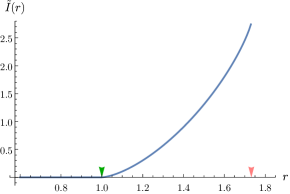
Right: Radial rate function , computed analytically from (5.21) and (5.4). The marked spots on the -axis correspond are the slopes of the asymptotes in the left diagram.
It turns out that the maximum is always attained for and , and equivalent points. At these points the function is easily evaluated as
| (5.21) |
The Legendre transform can be evaluated analytically (see Figure 6), but the expression is not very enlightening. We have for , i.e., in the propagation region, and for , which corresponds to the largest jump vector (and equivalents) visible in (5.15) as the appearance of trigonometric power . This corresponds to the trivial bound in Lemma 4.1. For intermediate we have, for example, , so that the probability for position outside a ball of radius after steps decays at least like .
Acknowledgements
The main idea and body of the paper originate from a visit of A.J. to Hannover in 2012. We decided to wrap up and complete it, because, to the best of our knowledge, it still provides the best result of its kind. The authors thank André Ahlbrecht for stimulating discussions on early drafts of this manuscript. C. Cedzich acknowledges partial support by the Deutsche Forschungsgemeinschaft (DFG, German Research Foundation) – 441423094.
References
- [1] A. Ahlbrecht, C. Cedzich, R. Matjeschk, V. B. Scholz, A. H. Werner, and R. F. Werner. Asymptotic behavior of quantum walks with spatio-temporal coin fluctuations. Quantum Inf. Process., 11(5):1219–1249, 2012. arXiv:1201.4839.
- [2] A. Ahlbrecht, H. Vogts, A. H. Werner, and R. F. Werner. Asymptotic evolution of quantum walks with random coin. J. Math. Phys., 52:042201, 2011. arXiv:1009.2019.
- [3] Y. Baryshnikov, W. Brady, A. Bressler, and R. Pemantle. Two-dimensional quantum random walk. J. Stat. Phys., 142:78–107, 2011. arXiv:0810.5495.
- [4] H. Baumgärtel. Analytic perturbation theory for matrices and operators. Birkhäuser, 1985.
- [5] M. V. Berry. Evanescent and real waves in quantum billiards and Gaussian beams. J. Phys. A: Math. Gen., 27(11):L391, 1994.
- [6] I. Byalinicki-Birula. Weyl, Dirac, and Maxwell equations on a lattice as unitary cellular automata. Phy. Rev. D, 49:6920–6927, 1994. arXiv:hep-th/9304070.
- [7] H. A. Carteret, M. E. H. Ismail, and B. Richmond. Three routes to the exact asymptotics for the one-dimensional quantum walk. J. Phys. A: Math. Gen., 36:8775–8795, 2003. arXiv:quant-ph/0303105.
- [8] H. A. Carteret, B. Richmond, and N. M. Temme. Evanescence in coined quantum walks. J. Phys. A: Math. Gen., 38:8641, 2005. arXiv:quant-ph/0506048.
- [9] P. Debye. Näherungsformeln für die Zylinderfunktionen für große Werte des Arguments und unbeschränkt veränderliche Werte des Index. Math. Ann., 67(4):535–558, 1909.
- [10] R. Ellis. Entropy, Large Deviations, and Statistical Mechanics. Springer, 1985.
- [11] H. Grauert and K. Fritzsche. Several complex variables. Springer, 1976.
- [12] G. Grimmett, S. Janson, and P. F. Scudo. Weak limits for quantum random walks. Phys. Rev. E, 69:026119, 2004. arXiv:quant-ph/0309135.
- [13] G. Harris and C. Martin. The roots of a polynomial vary continuously as a function of the coefficients. Proc. Am. Math. Soc, 100:390–392, 1987.
- [14] T. Kato. Perturbation theory for linear operators. Springer, Berlin, 1984.
- [15] N. Konno. A new type of limit theorems for the one-dimensional quantum random walk. J. Math. Soc. Jpn., 57(4):1179–1195, 2005. arXiv:quant-ph/0206103.
- [16] E. H. Lieb and D. W. Robinson. The finite group velocity of quantum spin systems. Commun. Math. Phys., 28(3):251–257, 1972.
- [17] E. Lukacs. Characteristic functions. Griffin. Hodder Arnold, 2 edition, 1970.
- [18] P. Lévy. Sur la détermination des lois de probabilité par leur fonctions caractéristiques. Cr. Hebd. Acad. Sci., pages 854–856, 1922.
- [19] P. Lévy. Théorie de l’addition des variables aléatoires. Monographies des probabilités. Gauthier-Villars, 1937.
- [20] P. Naaijkens. Quantum Spin Systems on Infinite Lattices: A Concise Introduction, volume 933 of Lecture Notes in Physics. Springer International Publishing, 2017.
- [21] B. Nachtergaele and R. Sims. Lieb-Robinson Bounds in Quantum Many-Body Physics. In Entropy and the quantum, volume 529 of Contemp. Math., pages 141–176. Amer. Math. Soc., Providence, RI, arXiv:1004.2086.
- [22] W. Rudin. Functional analysis. McGraw-Hill, New York, 2nd ed edition, 1991.
- [23] T. Sunada and T. Tate. Asymptotic behavior of quantum walks on the line. J. Funct. Anal., 262:2608–2645, 2012. arXiv:1108.1878.
- [24] K. Watabe, N. Kobayashi, M. Katori, and N. Konno. Limit distributions of two-dimensional quantum walks. Phys. Rev. A, 77:062331, 2008. arXiv:0802.2749.
- [25] S. Weinberg. Gauge and global symmetries at high temperature. Phys. Rev. D, 9(12):3357–3378, 1974.
- [26] W. Wong. Continuity of the infimum. https://williewong.wordpress.com/2011/11/01/continuity-of-the-infimum/, downloaded 22/07/2018.
Appendix A Continuity of the supremum
In this appendix we prove the following topological Lemma. The proof is taken and adapted from [26] and, besides completeness, is stated here to prevent the fleeting nature of blog posts:
Lemma A.1.
Let be topological spaces with compact, and let be (jointly) continuous. Then is well-defined and continuous.
Proof.
We prove the statement in three steps: first, for fixed , is continuous (by assumption) and bounded (since is compact). Therefore, .
Next, note that for the open sets and form a subbase for the topology on (the finite intersections of these sets form a basis for the standard topology on , see e.g. [22, Appendix A2]). Thus, the statement of the lemma follows from the openness of and .
Let be the canonical projection onto the first factor, which is open and continuous by definition. Clearly, , so that the continuity of implies that is open for any .
To show that also is open we use the compactness of : first, note that implies that for all (by definition of ). But this is just saying that the set
is open. This implies that for every and every there is a neighbourhood that is contained in (by the definition of openness). Since is compact, a finite subset labels such boxes that cover , and hence
This implies that is open, where for all . ∎