Conjugate radius, volume comparison and rigidity

Abstract.

In this paper, we prove conjugate radius estimate, volume comparison and rigidity theorems for Kähler manifolds with various curvature conditions.

1. Introduction

Comparison theorems are crucial tools for understanding geometric concepts in differential geometry. Let $(M,g)$ be a complete $n$-dimensional Riemannian manifold with Ricci curvature $\mathrm{Ric}(g)\geq(n-1)g$. Myers [Mye41] established the diameter comparison theorem that $\mathrm{diam}(M,g)\leq\mathrm{diam}({\mathbb{S}}^{n},g_{\mathrm{can}})=\pi$. Moreover, Cheng [Che75] obtained the diameter rigidity theorem, which states that if the diameter $\mathrm{diam}(M,g)=\mathrm{diam}({\mathbb{S}}^{n},g_{\mathrm{can}})$, then $(M,g)$ is isometric to the round sphere. Furthermore, the Bishop-Gromov volume comparison theorem (e.g. [BC64], [Gro07], [CE08]) asserts that $\mathrm{Vol}(M,g)\leq\mathrm{Vol}({\mathbb{S}}^{n},g_{\mathrm{can}})$, and the identity holds if and only if $(M,g)$ is isometric to the round sphere. In [CC97], Cheeger and Colding obtained similar rigidity theorems for volume gaps. For more details along this comprehensive topic, we refer to [Wei07] and the references therein.

There are many notable extensions on complete Kähler manifolds. For instance, Li and Wang [LW05] obtained diameter comparison and volume comparison theorems in the case that the holomorphic bisectional curvature has a positive lower bound $\mathrm{HBSC}\geq 1$. More recently, Datar and Seshadri [DS23] established the diameter rigidity theorem, which states that if $\mathrm{HBSC}\geq 1$ and $\mathrm{diam}(M,g)=\mathrm{diam}({\mathbb{C}}{\mathbb{P}}^{n},\omega_{\mathrm{FS}})$, then $(M,\omega_{g})$ is isometrically biholomorphic to $({\mathbb{C}}{\mathbb{P}}^{n},\omega_{\mathrm{FS}})$. This is achieved by using Siu-Yau’s solution to the Frankel conjecture [SY80] and an interesting monotonicity formula for Lelong numbers on ${\mathbb{C}}{\mathbb{P}}^{n}$ ([Lot21]). Similar results were proved in [TY12] and [LY18] with some extra conditions. On the other hand, utilizing entirely different techniques from algebraic geometry (e.g. [Fuj18]), Zhang [Zha22] obtained volume comparison and rigidity theorems under the assumption $\mathrm{Ric}(\omega)\geq(n+1)\omega$.

It is also an interesting topic to investigate diameter comparsion, volume comparison and rigidity theorems for complete Kähler manifolds with positive holomorphic sectional curvature. Tsukamoto proved in [Tsu57] that if a complete Kähler manifold $(M,\omega_{g})$ has holomorphic sectional curvature $\mathrm{HSC}\geq 2$, then $M$ is compact, simply connected, and $\mathrm{diam}(M,g)\leq\mathrm{diam}({\mathbb{C}}{\mathbb{P}}^{n},\omega_{\mathrm{FS}})$. Recently, Ni and Zheng [NZ18] obtained interesting Laplacian comparison and volume comparison theorems by assuming $\mathrm{HSC}\geq 2$ and orthogonal Ricci curvature $\mathrm{Ric}^{\perp}\geq(n-1)$.

In this paper, we derive volume comparison and rigidity theorems for Kähler manifolds under various curvature conditions. Additionally, we establish conjugate radius and injectivity radius estimates and the corresponding rigidity theorems.

For the reader’s convenience, we fix some terminologies. Let $(M,g)$ be a complete Riemannian manifold. For a unit vector $v\in T_{p}M$, $c_{v}$ is the smallest number $t_{0}>0$ such that $\gamma(t_{0})$ is conjugate to $p$ along the geodesic $\gamma(t)=\exp_{p}(tv)$. The conjugate radius of $p$ and the conjugate radius of $(M,g)$ are defined as

$$\mathrm{conj}(M,p):=\inf_{v\in T_{p}M,\,|v|=1}c_{v}\quad\mbox{and}\quad\mathrm{conj}(M,g):=\inf_{p\in M}\mathrm{conj}(M,p).$$

The first main result of this paper is the following volume comparison and rigidity theorem for Kähler manifolds with positive holomorphic sectional curvature.

Theorem 1.1.

Let $(M,\omega_{g})$ be a complete Kähler manifold with $\mathrm{HSC}\geq 2$. If there exists some point $p\in M$ such that $\mathrm{conj}(M,p)\geq\pi/\sqrt{2}$, then

(1.1) $$\mathrm{Vol}\left(M,\omega_{g}\right)\leq\mathrm{Vol}\left({\mathbb{C}}{\mathbb{P}}^{n},\omega_{\mathrm{FS}}\right),$$

and the identity holds if and only if $(M,\omega_{g})$ is isometrically biholomorphic to $({\mathbb{C}}{\mathbb{P}}^{n},\omega_{\mathrm{FS}})$.

This result is obtained by utilizing relationships between the RC-positivity proposed in [Yan18] and the conjugate radius estimate derived from the index theorem. The second named author established in [Yan18] that compact Kähler manifolds with positive holomorphic sectional curvature are projective and rationally connected, which confirmed affirmatively a conjecture proposed by S.-T. Yau in [Yau82, Problem 47], and such manifolds are not necessarily ${\mathbb{C}}{\mathbb{P}}^{n}$. The main difficulty in achieving volume comparison and rigidity theorems for compact Kähler manifolds with $\mathrm{HSC}>0$ is that the holomorphic sectional curvature is too weak to obtain Laplacian comparison type theorems (see Problem 3.5). Actually, we derive extra curvature relation from the lower bound of the conjugate radius at some point. Moreover, we establish (global) conjugate radius and injective radius estimates for such manifolds.

Theorem 1.2.

Let $(M,\omega_{g})$ be a complete Kähler manifold with $\mathrm{HSC}\geq 2$. Then

(1.2) $$\mathrm{inj}(M,g)=\mathrm{conj}(M,g)\leq\frac{\pi}{\sqrt{2}},$$

and the identity holds if and only if $(M,\omega_{g})$ is isometrically biholomorphic to $({\mathbb{C}}{\mathbb{P}}^{n},\omega_{\mathrm{FS}})$.

By using perturbations of $({\mathbb{C}}{\mathbb{P}}^{n},\omega_{\mathrm{FS}})$, it is easy to see that there exists a compact Kähler manifold $M$ with $\mathrm{HSC}\geq 2$ and $\mathrm{conj}(M,g)\leq\varepsilon<\pi/\sqrt{2}$, but there exists a point $p\in M$ such that $\mathrm{conj}(M,p)\geq\pi/\sqrt{2}$. Hence, the conditions in Theorem 1.1 cannot be implied by those in Theorem 1.2. On the other hand, Theorem 1.2 is a generalization of classical results obtained in [Kli59] and [Gre63] (see also [AM94]) for Riemannian manifolds. Indeed, if $(M,g)$ is a compact Riemannian manifold with scalar curvature $\geq n(n-1)$, Green [Gre63] proved that the conjugate radius $\mathrm{conj}(M,g)\leq\pi$, and the identity holds if and only if $(M,g)$ is isometric to the round sphere. We also obtain the following extension in Kähler geometry.

Theorem 1.3.

Let $(M,\omega_{g})$ be a compact Kähler manifold of complex dimension $n$. Then

(1.3) $$\frac{4a^{2}}{\pi(n+1)!}\int_{M}c_{1}(M)\wedge[\omega_{g}]^{n-1}\leq\mathrm{Vol}(M,\omega_{g}),$$

where $a$ is the conjugate radius of $(M,g)$. Moreover, the identity holds if and only if $(M,\omega_{g})$ is isometrically biholomorphic to $\left({\mathbb{C}}{\mathbb{P}}^{n},\frac{2a^{2}}{\pi^{2}}\omega_{\mathrm{FS}}\right)$.

It is well-known that if $(M,g)$ is a complete Riemannian manifold with non-positive sectional curvature, then $\mathrm{conj}(M,g)=+\infty$. In Theorem 1.3, the conjugate radius $a$ can also be $+\infty$, and in this case we have $\int_{M}c_{1}(M)\wedge[\omega_{g}]^{n-1}\leq 0$. Note also that Zhu established in [Zhu22] some interesting results on the geometry of positive scalar curvature on complete non-compact Riemannian manifolds with non-negative Ricci curvature, which can also be extended to Kähler manifolds by using (total) scalar curvature. As an application of Theorem 1.3, one has

Corollary 1.4.

Let $(M,\omega_{g})$ be a compact Kähler manifold of complex dimension $n$. If the scalar curvature of $(M,\omega_{g})$ satisfies $s\geq n(n+1)$, then

(1.4) $$\mathrm{conj}(M,g)\leq\frac{\pi}{\sqrt{2}},$$

and the identity holds if and only if $(M,\omega_{g})$ is isometrically biholomorphic to $({\mathbb{C}}{\mathbb{P}}^{n},\omega_{\mathrm{FS}})$.

As another application of Theorem 1.3, we give a criterion for finiteness of $\mathrm{conj}(M,g)$ by using RC-positivity.

Theorem 1.5.

Let $M$ be a compact Kähler manifold. If the anti-canonical line bundle $K_{M}^{-1}$ is RC-positive, then for any Kähler metric $\omega_{g}$ on $M$,

$$\mathrm{conj}(M,g)<+\infty.$$

Recall that the anti-canonical line bundle $K^{-1}_{M}$ of a compact complex manifold $M$ is called RC-positive if there exists a Hermitian metric $\omega$ on $TM$ such that the first Chern-Ricci curvature $\mathrm{Ric}^{(1)}(\omega)$ has a positive eigenvalue at each point $p\in M$. It is proved in [Yan19a] and [Yan19b] that $K_{M}^{-1}$ is RC-positive if and only if $K_{M}$ is not a pseudo-effective line bundle. Consequently, any Kähler metric on a uniruled algebraic manifold has finite conjugate radius. We also observe that the converse of Theorem 1.5 is not valid in general. Actually, if $M$ is a complete intersection of two generic hypersurfaces in ${\mathbb{C}}{\mathbb{P}}^{4}$ whose degrees are greater than $35$, it is shown in [Bro14, Corollary 4.13] that $M$ has ample cotangent bundle and so $K_{M}$ is pseudo-effective. Moreover, since $M$ is simply connected ([Sha13, pp. 221–222]), any metric $g$ on $M$ must have finite conjugate radius. Otherwise, $M$ would be diffeomorphic to ${\mathbb{R}}^{4}$.

Finally, we establish volume comparison and rigidity theorems for complete Kähler manifolds with positive orthogonal holomorphic bisectional curvature (OHBSC), which generalize results in [LW05].

Theorem 1.6.

Let $(M,\omega_{g})$ be a complete Kähler manifold of dimension $n\geq 2$. If $\mathrm{OHBSC}\geq 1$, then $M$ is compact and

(1.5) $$\mathrm{Vol}(M,\omega_{g})\leq\mathrm{Vol}({\mathbb{C}}{\mathbb{P}}^{n},\omega_{\mathrm{FS}}),$$

and the identity holds if and only if $(M,\omega_{g})$ is isometrically biholomorphic to $({\mathbb{C}}{\mathbb{P}}^{n},\omega_{\mathrm{FS}})$.

The proof of Theorem 1.6 relies on classical results in [Mok88], [Che07], [GZ10], [CT12] and [FLW17] that a compact Kähler manifold with positive orthogonal holomorphic bisectional curvature must be biholomorphic to ${\mathbb{C}}{\mathbb{P}}^{n}$. For more discussions on compact Kähler manifolds with positive holomorphic sectional curvature, we refer to [YZ19], [Yan20], [Yan21], [Ni21], [Mat22], [NZ22], [LZZ21+], [ZZ23+] and the references therein.

Acknowledgements. The second named author would like to thank Bing-Long Chen, Jixiang Fu and Valentino Tosatti for helpful discussions. He would also like to thank Professor Shing-Tung Yau and Professor Kefeng Liu for their support, encouragement and stimulating discussions over many years. The second named author is partially supported by National Key R&D Program of China 2022YFA1005400 and NSFC grants (No. 12325103, No. 12171262 and No. 12141101).

2. Estimates of conjugate radius

In this section we obtain conjugate radius estimates for compact Kähler manifolds and establish Theorem 1.3, Corollary 1.4 and Theorem 1.5. Let $(M,g)$ be a complete Riemannian manifold. For each $t\in{\mathbb{R}}$, there is a flow induced by geodesics of $(M,g)$

(2.1) $$\varphi_{t}:TM\to TM,\ \ \varphi_{t}(p,v)=\left(\gamma_{v}(t),\gamma_{v}^{\prime}(t)\right)$$

where $v\in T_{p}M$ and $\gamma_{v}(t)=\exp_{p}(tv)$. We also write it as $\varphi_{t}(v)=\gamma^{\prime}_{v}(t)$ for simplicity. We shall show that this flow is volume preserving, i.e., the determinant of the Jacobian map of $\varphi_{t}$ with respect to the induced Sasaki metric on $TM$ is $1$. Let’s describe the set up briefly and we refer to [Gre63, Lemma 3.1] and [Gro16] for more details. Let $\pi:TM\to M$ be the projection of the tangent bundle. There is a natural bundle map

(2.2) $$C:TTM\to TM$$

which is defined as follows. Let $m$ be a point in $TM$.

1. For $Z\in T_{m}TM$, there exists a smooth curve $V:(-\varepsilon,\varepsilon)\to TM$ such that $V(0)=m$ and $V^{\prime}(0)=Z$.

2. Let $\gamma=\pi\circ V:(-\varepsilon,\varepsilon)\rightarrow M$ be a curve. The map $C$ is given by

   (2.3) $$C(m,Z)=\left(\pi(m),\widehat{\nabla}_{\left.\frac{d}{dt}\right|_{t=0}}\left(\gamma^{*}V\right)\right)$$

   where $\widehat{\nabla}$ is the pullback Levi-Civita connection along $\gamma:(-\varepsilon,\varepsilon)\rightarrow M$.

It is easy to see that the bundle map $C$ is well-defined and smooth. Moreover,

$${\mathcal{H}}:=\ker C\quad\mbox{and}\quad{\mathcal{V}}:=\ker\pi_{*}$$

are subbundles of $TTM$ satisfying $TTM={\mathcal{H}}\oplus{\mathcal{V}}$. It is well-known that there exists a unique Riemannian metric $\widehat{g}$ on smooth manifold $TM$, which is called the Sasaki metric, such that ${\mathcal{H}}\perp{\mathcal{V}}$ and for all $p\in M$ and $v\in T_{p}M$, and the maps

(2.4) $$\pi_{*}:H_{(p,v)}\to T_{p}M\quad\mbox{and}\quad C:{\mathcal{V}}_{(p,v)}\to T_{p}M$$

are linear isometries where $T_{p}M$ is endowed with the Euclidean metric induced by $g$. Let $\widehat{g}_{p}$ be the induced metric on the submanifold $T_{p}M$ of $(TM,\widehat{g})$.

Lemma 2.1.

$\widehat{g}_{p}$ coincides with the Euclidean metric on $T_{p}M$ induced by $g$.

Proof.

Fix two points $v,w\in T_{p}M$ and set

$$V(t)=v+tw:{\mathbb{R}}\rightarrow T_{p}M\subset TM.$$

Then $\gamma:=\pi\circ V:{\mathbb{R}}\rightarrow M$ is a constant, i.e. $\gamma(t)\equiv p$. Therefore $V^{\prime}(0)\in T_{(p,v)}TM$ and it is in

$$\ker\pi_{*(p,v)}={\mathcal{V}}_{(p,v)}.$$

Since $V(t)$ is also a curve in $T_{p}M$, one can identify $V^{\prime}(0)\in T_{v}(T_{p}M)\subset T_{(p,v)}TM$ and

(2.5) $$|V^{\prime}(0)|_{\widehat{g}_{p}}=|V^{\prime}(0)|_{\widehat{g}}.$$

Let $\{x^{i}\}$ be local coordinates near $p\in M$, and $e_{i}=\frac{\partial}{\partial x^{i}}$ around $p$. We write $v=v^{i}e_{i}(p)$ and $w=w^{j}e_{j}(p)$. Then $\left(\gamma^{*}V\right)(t)=\left(v^{i}+tw^{i}\right)\widehat{e_{i}}$ where $\widehat{e_{i}}=\gamma^{*}e_{i}$ and

(2.6) $$\widehat{\nabla}_{\left.\frac{d}{dt}\right|_{t=0}}\left(\gamma^{*}V\right)=w^{i}\widehat{e_{i}}(0)+v^{i}\widehat{\nabla}_{\left.\frac{d}{dt}\right|_{t=0}}\widehat{e_{i}}=w^{i}\widehat{e_{i}}(0)=w$$

where we use the fact that $\gamma(t)\equiv p$. Therefore,

(2.7) $$C(v,V^{\prime}(0))=\left(p,\widehat{\nabla}_{\left.\frac{d}{dt}\right|_{t=0}}\left(\gamma^{*}V\right)\right)=(p,w).$$

That is $C(V^{\prime}(0))=w$. Since $C:{\mathcal{V}}_{(p,v)}\to T_{p}M$ is a linear isometry, one has

(2.8) $$|V^{\prime}(0)|_{\widehat{g}_{p}}=|V^{\prime}(0)|_{\widehat{g}}=|w|_{g}.$$

By using the identification $T_{v}(T_{p}M)\cong T_{p}M$, one deduces that the Riemannian metric $\widehat{g}_{p}$ on $T_{p}M$ coincides with the Euclidean metric on $T_{p}M$ induced by $g$. ∎

Let $(M,g)$ be a compact and oriented Riemannian manifold and $SM$ be the unit tangent bundle of $M$. For simplicity, the induced metric on the submanifold $SM$ of $TM$ is denoted by $\widehat{g}$ and the induced metric on $S_{p}M$ is also denoted by $\widehat{g}_{p}$. By using Lemma 2.1, one obtains the following well-known lemma (e.g. [Gro16]) in Riemannian geometry.

Lemma 2.2.

For each $f\in C^{\infty}(SM,{\mathbb{R}})$, one has

(2.9) $$\int_{SM}f\,d\mathrm{vol}_{\widehat{g}}=\int_{M}\left(\int_{S_{p}M}\left.f\right|_{S_{p}M}\,d\mathrm{vol}_{\widehat{g}_{p}}\right)d\mathrm{vol}_{g}=\int_{SM}f\circ\varphi_{t}\,d\mathrm{vol}_{\widehat{g}}.$$

We introduce a complex analog of the flow (2.1) on a compact Kähler manifold $(M,\omega_{g})$. For each $t\in{\mathbb{R}}$, there is an induced flow on the holomorphic tangent bundle

(2.10) $$\psi_{t}=\Phi\circ\varphi_{t}\circ\Phi^{-1}:T^{1,0}M\to T^{1,0}M$$

where the identification $\Phi:T_{\mathbb{R}}M\to T^{1,0}M$ is given by $\Phi(v)=\frac{1}{\sqrt{2}}\left(v-\sqrt{-1}Jv\right)$ and $\varphi_{t}$ is defined in (2.1). There is an induced Riemannian metric on smooth manifold $T^{1,0}M$ which is given by

(2.11) $$\widetilde{g}=(\Phi^{-1})^{*}\widehat{g}$$

where $\widehat{g}$ is the Sasaki metric on the real tangent bundle $T_{\mathbb{R}}M$ of $M$. Let $UM$ be the unit holomorphic tangent bundle of $T^{1,0}M$, $\widetilde{g}$ be the Riemannian metric on $UM$ induced by $(T^{1,0}M,\widetilde{g})$, and $\widetilde{g}_{p}$ be the Riemannian metric on the submanifold $U_{p}M\subset T_{p}^{1,0}M$ which coincides with the Euclidean metric on $T^{1,0}_{p}M$ induced by $g$ as shown in Lemma 2.1.

Proposition 2.3.

For each $f\in C^{\infty}(UM,{\mathbb{R}})$, one has

(2.12) $$\int_{UM}f\,d\mathrm{vol}_{\widetilde{g}}=\int_{M}\left(\int_{U_{p}M}\left.f\right|_{U_{p}M}\,d\mathrm{vol}_{\widetilde{g}_{p}}\right)d\mathrm{vol}_{g}=\int_{UM}f\circ\psi_{t}\,d\mathrm{vol}_{\widetilde{g}}.$$

Proof.

Since $\Phi$ is a smooth isometry which sends $SM$ to $UM$, by Lemma 2.2, we have

$$\int_{UM}f\circ\psi_{t}\,d\mathrm{vol}_{\widetilde{g}} = \int_{SM}f\circ\psi_{t}\circ\Phi\,d\mathrm{vol}_{\widehat{g}}=\int_{SM}f\circ\Phi\circ\varphi_{t}\,d\mathrm{vol}_{\widehat{g}}$$

$$= \int_{SM}f\circ\Phi\,d\mathrm{vol}_{\widehat{g}}=\int_{UM}f\,d\mathrm{vol}_{\widetilde{g}}.$$

Moreover, by integration formula (2.9) , one has

$$\int_{UM}f\,d\mathrm{vol}_{\widetilde{g}}=\int_{SM}f\circ\Phi\,d\mathrm{vol}_{\widehat{g}}=\int_{M}\left(\int_{S_{p}M}\left.f\circ\Phi\right|_{S_{p}M}\,d\mathrm{vol}_{\widehat{g}_{p}}\right)d\mathrm{vol}_{g}.$$

Note that the restriction $\Phi:(S_{p}M,\widehat{g}_{p})\to(U_{p}M,\widetilde{g}_{p})$ is a smooth isometry, and so

$$\int_{U_{p}M}\left.f\right|_{U_{p}M}\,d\mathrm{vol}_{\widetilde{g}_{p}}=\int_{S_{p}M}\left.f\circ\Phi\right|_{S_{p}M}\,d\mathrm{vol}_{\widehat{g}_{p}}.$$

Therefore we obtain the conclusion. ∎

Before giving the proof of Theorem 1.3, we need some algebraic calculations.

Lemma 2.4.

Let $({\mathbb{S}}^{2n-1},g_{\mathrm{can}})\subset{\mathbb{C}}^{n}$ be the round sphere. Then

$$\int_{{\mathbb{S}}^{n-1}}\xi^{i}\overline{\xi^{j}}\xi^{k}\overline{\xi^{\ell}}\,d\mathrm{vol}_{g_{\mathrm{can}}}=\frac{\mathrm{Vol}({\mathbb{S}}^{2n-1})}{n(n+1)}\left(\delta_{ij}\delta_{k\ell}+\delta_{i\ell}\delta_{jk}\right)$$

where $\xi=(\xi^{1},\cdots,\xi^{n})\in{\mathbb{S}}^{2n-1}\subset{\mathbb{C}}^{n}$.

Lemma 2.5.

Let $(M^{n},\omega_{g})$ be a Kähler manifold. Fix a point $p\in M$ and let $U_{p}M=\left\{v\in T^{1,0}_{p}M:|v|_{g}=1\right\}$. Then

(2.13) $$2s(p)=\frac{n(n+1)}{\mathrm{Vol}({\mathbb{S}}^{2n-1})}\int_{U_{p}M}R(V,\overline{V},V,\overline{V})\,d\mathrm{vol}_{\widetilde{g}_{p}}$$

where $\widetilde{g}_{p}$ is the induced metric on $T^{1,0}_{p}M$.

Proof.

Let $\{e_{i}\}_{i=1}^{n}$ be an unitary basis of $T^{1,0}_{p}M$, and $R_{i\overline{j}k\overline{\ell}}:=R(e_{i},\overline{e_{j}},e_{k},\overline{e_{\ell}})$. If $\xi=(\xi^{1},\cdots,\xi^{n})\in{\mathbb{S}}^{2n-1}\subset{\mathbb{C}}^{n}$ and $V=\xi^{i}e_{i}$, then by Lemma 2.4,

$$\int_{U_{p}M}R(V,\overline{V},V,\overline{V})\,d\mathrm{vol}_{\widetilde{g}_{p}} = \int_{{\mathbb{S}}^{2n-1}}R_{i\overline{j}k\overline{\ell}}\xi^{i}\overline{\xi^{j}}\xi^{k}\overline{\xi^{\ell}}\,d\mathrm{vol}_{g_{\mathrm{can}}}$$

$$= \frac{\mathrm{Vol}({\mathbb{S}}^{2n-1})}{n(n+1)}\sum_{i,j,k,\ell=1}^{n}R_{i\overline{j}k\overline{\ell}}\left(\delta_{ij}\delta_{k\ell}+\delta_{i\ell}\delta_{jk}\right)$$

$$= \frac{\mathrm{Vol}({\mathbb{S}}^{2n-1})}{n(n+1)}2s(p)$$

where $s(p)$ is the scalar curvature of the Kähler metric at point $p\in M$. ∎

Proof of Theorem 1.3. Suppose that $\mathrm{conj}(M,g)=a<+\infty$. Let $\gamma:[0,a]\to M$ be an arbitrary unit speed geodesic with $\gamma(0)=p$ and $\gamma^{\prime}(0)=v\in T_{p}M$. Consider a normal variational vector field along $\gamma$

$$W(t)=\sin\left(\frac{\pi t}{a}\right)J\gamma^{\prime}(t).$$

Since $\mathrm{conj}(M,g)=a$, by the index form theorem, one has

(2.14) $$I_{\gamma}(W,W)=\int_{0}^{a}\left\{\left\langle\widehat{\nabla}_{\frac{d}{dt}}W,\widehat{\nabla}_{\frac{d}{dt}}W\right\rangle-R(W,\gamma^{\prime},\gamma^{\prime},W)\right\}dt\geq 0.$$

This implies

(2.15) $$\int_{0}^{a}\sin^{2}\left(\frac{\pi t}{a}\right)R(J\gamma^{\prime},\gamma^{\prime},\gamma^{\prime},J\gamma^{\prime})\,dt\leq\int_{0}^{a}\frac{\pi^{2}}{a^{2}}\cos^{2}\left(\frac{\pi t}{a}\right)\,dt=\frac{\pi^{2}}{2a}.$$

By using the index form theorem again, one deduces that the identity holds if and only if $W(t)$ is a Jacobi field along $\gamma$. We write $V_{t}:=\frac{1}{\sqrt{2}}\left(\gamma^{\prime}(t)-\sqrt{-1}J\gamma^{\prime}(t)\right)$ for each $t\in[0,a]$, and set $V:=\frac{1}{\sqrt{2}}\left(v-\sqrt{-1}Jv\right)$. Then for each $t\in[0,a]$, one has

$$\psi_{t}V=\Phi\circ\varphi_{t}\circ\Phi^{-1}(V)=\Phi\circ\varphi_{t}(v)=\Phi(\gamma^{\prime}(t))=V_{t}.$$

On the other hand, a straightforward calculation shows

(2.16) $$R(J\gamma^{\prime},\gamma^{\prime},\gamma^{\prime},J\gamma^{\prime})(t)=R(V_{t},\overline{V}_{t},V_{t},\overline{V}_{t})=R(\psi_{t}V,\overline{\psi_{t}V},\psi_{t}V,\overline{\psi_{t}V}).$$

Therefore, (2.15) is equivalent to

(2.17) $$\int_{0}^{a}\sin^{2}\left(\frac{\pi t}{a}\right)R(\psi_{t}V,\overline{\psi_{t}V},\psi_{t}V,\overline{\psi_{t}V})\,dt\leq\frac{\pi^{2}}{2a}.$$

Since $p$ and $v$ are arbitrary, one deduces that (2.17) holds for all $p\in M$ and $V\in U_{p}M$. By using Proposition 2.3, one can integrate (2.17) over $UM$ and obtain

$$\frac{\pi^{2}}{2a}\mathrm{Vol}(M,\omega_{g})\mathrm{Vol}({\mathbb{S}}^{2n-1}) = \int_{UM}\frac{\pi^{2}}{2a}d\mathrm{vol}_{\widetilde{g}}$$

$$\geq \int_{UM}\left(\int_{0}^{a}\sin^{2}\left(\frac{\pi t}{a}\right)R(\psi_{t}V,\overline{\psi_{t}V},\psi_{t}V,\overline{\psi_{t}V})\,dt\right)d\mathrm{vol}_{\widetilde{g}}$$

$$= \int_{0}^{a}\sin^{2}\left(\frac{\pi t}{a}\right)\left(\int_{UM}R(\psi_{t}V,\overline{\psi_{t}V},\psi_{t}V,\overline{\psi_{t}V})\,d\mathrm{vol}_{\widetilde{g}}\right)dt.$$

Note that for each $t\in{\mathbb{R}}$, by Proposition 2.3 and Lemma 2.5, one has

$$\int_{UM}R(\psi_{t}V,\overline{\psi_{t}V},\psi_{t}V,\overline{\psi_{t}V})\,d\mathrm{vol}_{\widetilde{g}} = \int_{UM}R(V,\overline{V},V,\overline{V})\,d\mathrm{vol}_{\widetilde{g}}$$

$$= \int_{M}\left(\int_{U_{p}M}R(V,\overline{V},V,\overline{V})\,d\mathrm{vol}_{\widetilde{g}_{p}}\right)d\mathrm{vol}_{g}$$

$$= \frac{\mathrm{Vol}({\mathbb{S}}^{2n-1})}{n(n+1)}\int_{M}2s\,d\mathrm{vol}_{g}$$

$$= \frac{4\pi\mathrm{Vol}({\mathbb{S}}^{2n-1})}{(n+1)!}\int_{M}c_{1}(M)\wedge[\omega_{g}]^{n-1}.$$

Therefore, one has

$$\frac{\pi^{2}}{2a}\mathrm{Vol}(M,\omega_{g})\mathrm{Vol}({\mathbb{S}}^{2n-1}) \geq \int_{0}^{a}\sin^{2}\left(\frac{\pi t}{a}\right)\,dt\cdot\frac{4\pi\mathrm{Vol}({\mathbb{S}}^{2n-1})}{(n+1)!}\int_{M}c_{1}(M)\wedge[\omega_{g}]^{n-1}$$

$$= \frac{2\pi a}{(n+1)!}\mathrm{Vol}({\mathbb{S}}^{2n-1})\int_{M}c_{1}(M)\wedge[\omega_{g}]^{n-1}.$$

Thus we obtain the inequality (1.3). Furthermore, suppose that the identity in (1.3) holds. One can deduce that the identity in (2.17) holds for all $p\in M$ and $V\in U_{p}M$. Moreover, the identity in (2.15) holds for any unit-speed geodesic $\gamma:[0,a]\to M$, and $W(t)=\sin(\pi t/a)J\gamma^{\prime}(t)$ is a Jacobi field along $\gamma$. This implies

$$\left\langle\widehat{\nabla}_{\frac{d}{dt}}\widehat{\nabla}_{\frac{d}{dt}}W+R(W,\gamma^{\prime})\gamma^{\prime},W\right\rangle(t)=\sin^{2}\left(\frac{\pi t}{a}\right)\left(-\frac{\pi^{2}}{a^{2}}+R(J\gamma^{\prime},\gamma^{\prime},\gamma^{\prime},J\gamma^{\prime})(t)\right)=0.$$

Therefore, for any $t\in(0,a)$,

$$R(J\gamma^{\prime},\gamma^{\prime},\gamma^{\prime},J\gamma^{\prime})(t)=\frac{\pi^{2}}{a^{2}}$$

and by continuity, one obtains $R(Jv,v,v,Jv)=\pi^{2}/a^{2}$ where $v=\gamma^{\prime}(0)\in T_{p}M$. Since $v$ and $p$ are arbitrary, we conclude that $(M,\omega_{g})$ has constant holomorphic sectional curvature $\pi^{2}/a^{2}$, and so $(M,\omega_{g})$ is isometrically biholomorphic to $\left({\mathbb{C}}{\mathbb{P}}^{n},\frac{2a^{2}}{\pi^{2}}\omega_{\mathrm{FS}}\right)$.

Suppose that $\mathrm{conj}(M,g)=+\infty$. Let $\alpha$ be an arbitrary positive number, and $\gamma:[0,\alpha]\to M$ be a unit-speed geodesic. Since $\mathrm{conj}(M,g)>\alpha$, by using the index form theorem, one has $I_{\gamma}(W,W)>0$ where $W(t)=\sin(\pi t/\alpha)J\gamma^{\prime}(t)$. By using similar arguments as above, one can show

$$\int_{0}^{\alpha}\sin^{2}\left(\frac{\pi t}{a}\right)R(J\gamma^{\prime},\gamma^{\prime},\gamma^{\prime},J\gamma^{\prime})\,dt<\frac{\pi^{2}}{2\alpha}.$$

We can repeat previous arguments and obtain

$$\frac{4\alpha^{2}}{\pi(n+1)!}\int_{M}c_{1}(M)\wedge[\omega_{g}]^{n-1}<\mathrm{Vol}(M,\omega_{g}).$$

Since $\alpha$ is arbitrary, we deduce that

(2.18) $$\int_{M}c_{1}(M)\wedge[\omega_{g}]^{n-1}\leq 0.$$

Hence, the inequality in (1.3) holds. Moreover, the identity in (1.3) can not hold. ∎

Proof of Corollary 1.4. Since the scalar curvature $s\geq n(n+1)$, one has

$$\int_{M}c_{1}(M)\wedge[\omega_{g}]^{n-1}\geq\frac{(n+1)!}{2\pi}\mathrm{Vol}(M,\omega_{g}).$$

Therefore, by Theorem 1.3, one deduces that $a<+\infty$ and

$$\frac{2a^{2}}{\pi^{2}}\mathrm{Vol}(M,\omega_{g})\leq\frac{4a^{2}}{\pi(n+1)!}\int_{M}c_{1}(M)\wedge[\omega_{g}]^{n-1}\leq\mathrm{Vol}(M,\omega_{g}).$$

This implies $a\leq\pi/\sqrt{2}$. Moreover, if $a=\pi/\sqrt{2}$, by the proof of Theorem 1.3, one can see that $(M,\omega_{g})$ is isometrically biholomorphic to $({\mathbb{C}}{\mathbb{P}}^{n},\omega_{\mathrm{FS}})$. ∎

Proof of Theorem 1.5.

Suppose there exists some Kähler metric $\omega_{g}$ on $M$ such that $\mathrm{conj}(M,g)=+\infty$. By the proof of Theorem 1.3, we deduce that

$$\int_{M}c_{1}(M)\wedge[\omega_{g}]^{n-1}\leq 0.$$

By [Yan19b, Theorem 1.1], we conclude that $K_{M}$ is pseudo-effective. However, by [Yan19a, Theorem 1.5], if $K_{M}^{-1}$ is RC-positive, then $K_{M}$ is not pseudoeffecive and this is a contradiction. ∎

3. Injectivity radius, volume comparison and rigidity theorems for holomorphic sectional curvature

In this section, we investigate the geometry of complete Kähler manifolds with positive holomorphic sectional curvature (HSC) and demonstrate Theorem 1.1 and Theorem 1.2. Let $(M,g)$ be a complete Riemannian manifold and $p\in M$. For small $r>0$, $B_{r}(p):=\exp_{p}\left(B_{r}(0)\right)$ is an open subset of $M$, and $\exp_{p}:B_{r}(0)\rightarrow B_{r}(p)$ is a diffeomorphism. The supremum of all such $r>0$ is called the injectivity radius of $M$ at $p$ and it is denoted by $\mathrm{inj}_{p}(M,g)$. The injectivity radius of $M$, denoted by $\mathrm{inj}(M,g)$, is $\inf_{p\in M}\mathrm{inj}_{p}(M,g)$. The following result is well-known and we refer to [dC92, pp. 274] and [Kli59].

Lemma 3.1.

Let $(M,g)$ be a complete Riemannian manifold and $p\in M$. Suppose that there exists some point $q\in\mathrm{cut}(p)$ such that $d(p,q)=d(p,\mathrm{cut}(p))=\ell$. Then one has

1. either $q$ is a conjugate point of $p$ along some minimizing geodesic from $p$ to $q$, or there are exactly two unit-speed minimizing geodesics from $p$ to $q$, say $\gamma_{1},\gamma_{2}:[0,\ell]\to M$ such that $\gamma_{1}^{\prime}(\ell)=-\gamma_{2}^{\prime}(\ell)$;

2. if in addition that $\mathrm{inj}_{p}(M,g)=\mathrm{inj}(M,g)$, and that $q$ is not conjugate to $p$ along any minimizing geodesic, then there is a closed unit-speed geodesic $\gamma:[0,2\ell]\to M$ such that $\gamma(0)=\gamma(2\ell)=p$ and $\gamma(\ell)=q$.

We first show that on a compact Kähler manifold with positive holomorphic sectional curvature, the conjugate radius and the injectivity radius are the same, which is an analog of the classical result in [Kli59] for even dimensional orientable compact Riemannian manifolds with positive sectional curvature.

Proposition 3.2.

Let $(M,\omega_{g})$ be a compact Kähler manifold with positive holomorphic sectional curvature. Then $\mathrm{inj}(M,g)=\mathrm{conj}(M,g)$.

Proof.

Suppose for the sake of contradiction that $\mathrm{inj}(M,g)<\mathrm{conj}(M,g)$. Since $M$ is compact, there exist $p\in M$ and $q\in\mathrm{cut}(p)$ such that $\ell:=d(p,q)=\mathrm{inj}(M,g)$. Since $\mathrm{inj}(M,g)<\mathrm{conj}(M,g)$, one deduces that $q$ is not conjugate to $p$ along any minimizing geodesic. Then by part $(2)$ of Lemma 3.1, there is a closed unit-speed geodesic $\gamma:[0,2\ell]\to M$ such that

$$\gamma(0)=\gamma(2\ell)=p,\quad\gamma(\ell)=q.$$

In the following, we shall construct a third minimal geodesic connecting $q$ and $p$, and by part $(1)$ of Lemma 3.1, this is a contradiction.

Consider the variation

$$\alpha:[0,1]\times[0,2\ell]\to M,\ \ \alpha(s,t)=\exp_{\gamma(t)}(s\cdot W(t)),$$

where $W(t)=J\gamma^{\prime}(t)$. Let $\overline{\nabla}$ and $\widehat{\nabla}$ be the pullback Levi-Civita connections on $\alpha^{*}TM$ and $\gamma^{*}TM$ respectively. The first variation of the arclength of $\gamma(t)$ gives

$$\left.\frac{d}{ds}\right|_{s=0}L\left(\alpha(s,\bullet)\right)=\left.\left\langle\gamma^{\prime},W\right\rangle\right|_{t=0}^{t=2\ell}-\int_{0}^{2\ell}\left\langle\widehat{\nabla}_{\frac{d}{dt}}\gamma^{\prime},W\right\rangle dt=0.$$

Since $\gamma^{\prime}(0)=\gamma^{\prime}(2\ell)$, $\alpha(s,0)=\alpha(s,2\ell)$ for all $s\in[0,1]$, and $\widehat{\nabla}_{\frac{d}{dt}}J\gamma^{\prime}=0$, the second variation of the arclength of $\gamma(t)$ is reduced to

$$\left.\frac{d^{2}}{ds^{2}}\right|_{s=0}L\left(\alpha(s,\bullet)\right) = \left.\left\langle\gamma^{\prime},\left.\left(\overline{\nabla}_{\frac{\partial}{\partial s}}\alpha_{*}\left(\frac{\partial}{\partial s}\right)\right)\right|_{s=0}\right\rangle\right|_{t=0}^{t=2\ell}-\int_{0}^{2\ell}R(J\gamma^{\prime},\gamma^{\prime},\gamma^{\prime},J\gamma^{\prime})\,dt$$

$$= -\int_{0}^{2\ell}R(J\gamma^{\prime},\gamma^{\prime},\gamma^{\prime},J\gamma^{\prime})\,dt<0.$$

This implies that $\gamma$ is a local maximum of the arc-length functional. We shall construct a minimal geodesic connecting $q$ and $p$. We write $\alpha_{s}(t)=\alpha(s,t)$, and it is clear that

$$L(\alpha_{s})<L(\gamma)=2\ell$$

for sufficiently small $s>0$. Let $p_{s}=\alpha_{s}(0)$, and $q_{s}=\alpha_{s}(t_{s})$ be a point on the curve $\alpha_{s}$ that maximizes the distance to $p_{s}$. By using this construction, one has

$$d(p_{s},q_{s})\leq\frac{1}{2}L(\alpha_{s})<\frac{1}{2}L(\gamma)=\ell=\mathrm{inj}(M,g)$$

for sufficiently small $s>0$. This implies that there exists a unique unit-speed minimal geodesic $\sigma_{s}:[0,\ell_{s}]\to M$ connecting $q_{s}$ and $p_{s}$.

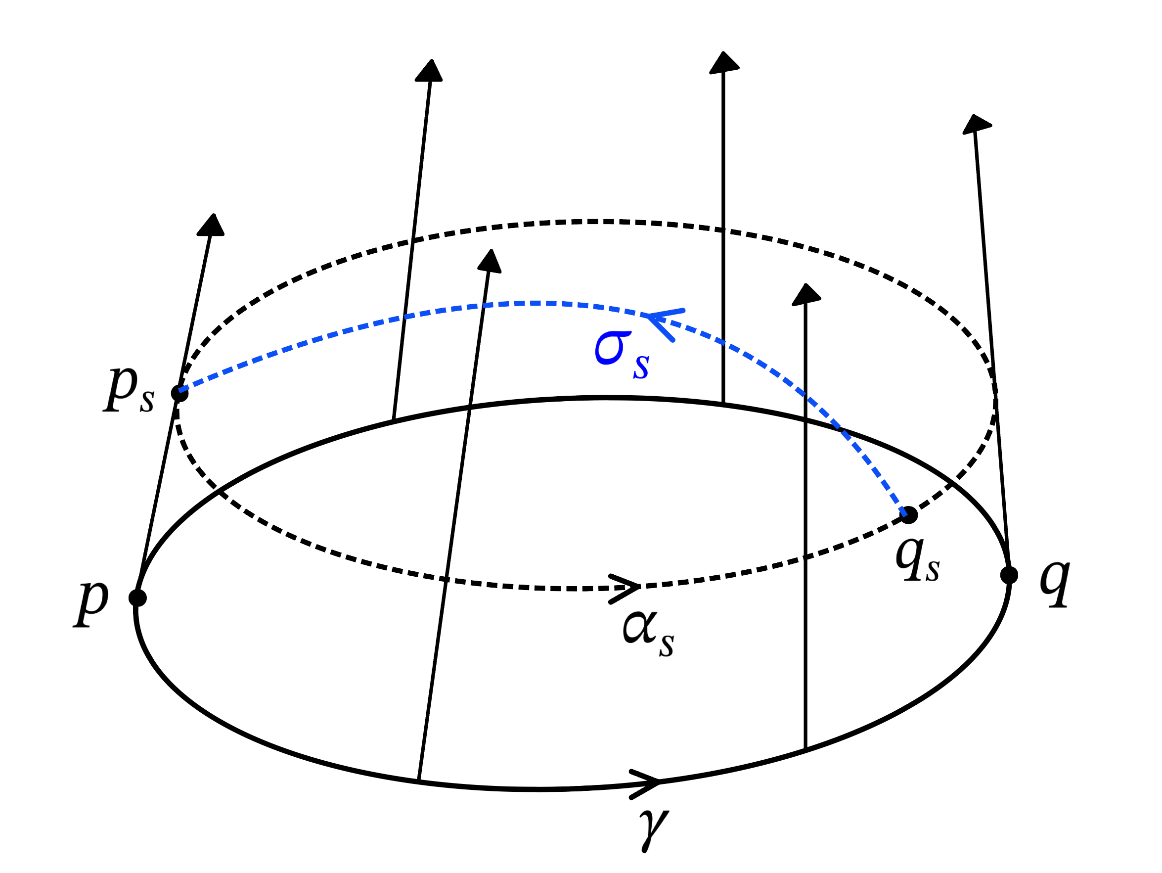
Figure 1. The variation of $\sigma_{s}$

Moreover, there exists a smooth variation

(3.1) $$\beta:(-\varepsilon,\varepsilon)\times[0,\ell_{s}]\to M$$

of $\sigma_{s}$ such that for each $\tau\in(-\varepsilon,\varepsilon)$, the curve $\beta(\tau,\bullet)$ is a minimal geodesic with

$$\beta(\tau,0)=\alpha_{s}(t_{s}+\tau)\quad\mbox{and}\quad\beta(\tau,\ell_{s})=p_{s}.$$

Let $U(t)$ be the variational vector field of $\beta$. Then

$$U(0)=\left.\frac{d}{d\tau}\right|_{\tau=0}\alpha_{s}(t_{s}+\tau)=\alpha_{s}^{\prime}(t_{s})\quad\mbox{and}\quad U(\ell_{s})=0.$$

By the definition of $q_{s}$, one has

$$L(\sigma_{s})=d(p_{s},q_{s})\geq d(p_{s},\alpha_{s}(t_{s}+\tau))=L(\beta(\tau,\bullet))$$

and so

(3.2) $$\left.\frac{d}{d\tau}\right|_{\tau=0}L\left(\beta(\tau,\bullet)\right)=0.$$

On the other hand, by the first variation formula, for sufficiently small $s>0$,

(3.3) $$0=\left.\frac{d}{d\tau}\right|_{\tau=0}L\left(\beta(\tau,\bullet)\right)=\left.\left\langle\sigma_{s}^{\prime},U\right\rangle\right|_{t=0}^{t=\ell_{s}}=-\left\langle\sigma_{s}^{\prime}(0),\alpha_{s}^{\prime}(t_{s})\right\rangle.$$

Let $\{s_{k}\}$ be a sequence in the open interval $(0,1)$ which converges to $0$. There exists a subsequence of $\{s_{k}\}$, which we also denote it by $\{s_{k}\}$, such that

$$\lim_{k\to\infty}t_{s_{k}}=t_{0}$$

for some $t_{0}\in[0,2\ell]$. Thus, one has

$$\lim_{k\to\infty}q_{s_{k}}=\lim_{k\to\infty}\alpha(s_{k},t_{s_{k}})=\alpha(0,t_{0})=\gamma(t_{0}).$$

Consider functions $f_{k}:[0,2\ell]\to{\mathbb{R}}$ and $f:[0,2\ell]\to{\mathbb{R}}$ given by

$$f_{k}(t)=d(\alpha_{s_{k}}(t),p_{s_{k}})\quad\mbox{and}\quad f(t)=d(\gamma(t),p).$$

One can see clearly that $f_{k}$ converges to $f$ uniformly, and

$$d(\gamma(t_{0}),p)=\lim_{k\to\infty}d(q_{s_{k}},p_{s_{k}})=\lim_{k\to\infty}\sup_{t\in[0,2\ell]}f_{k}(t)=\sup_{t\in[0,2\ell]}f(t)=\ell.$$

Since $q$ is the only point on $\gamma$ that maximizes the distance to $p$, one deduces that

(3.4) $$\lim_{k\to\infty}t_{s_{k}}=t_{0}=\ell,\quad\lim_{k\to\infty}d(q_{s_{k}},p_{s_{k}})=\lim_{k\to\infty}\ell_{s_{k}}=\ell,$$

and so

$$\lim_{k\to\infty}\sigma_{s_{k}}(0)=\lim_{k\to\infty}q_{s_{k}}=\gamma(\ell)=q.$$

Furthermore, by compactness of the unit tangent bundle, there exists a subsequence of $\{s_{k}\}$, which is also denoted by $\{s_{k}\}$, such that

(3.5) $$\lim_{k\to\infty}\sigma_{s_{k}}^{\prime}(0)=w$$

for some $w\in T_{q}M$. We define a unit-speed geodesic

(3.6) $$\sigma:[0,\ell]\to M,\ \ \ \sigma(t)=\exp_{q}(tw).$$

By continuity of the exponential map, one has

$$\sigma(\ell)=\lim_{k\to\infty}\sigma_{s_{k}}(\ell)=\lim_{k\to\infty}\sigma_{s_{k}}(\ell_{s_{k}})=\lim_{k\to\infty}p_{s_{k}}=p.$$

Thus, $\sigma$ is also a minimal geodesic connecting $q$ and $p$. Moreover, by (3.3), (3.4) and (3.5), one deduces that

$$0=\lim_{k\to\infty}\left\langle\sigma_{s_{k}}^{\prime}(0),\alpha_{s_{k}}^{\prime}(t_{s_{k}})\right\rangle=\left\langle\sigma^{\prime}(0),\gamma^{\prime}(\ell)\right\rangle.$$

Hence, $\sigma$ is a minimal geodesic connecting $q$ and $p$, which is different from two minimal geodesics connecting $q$ and $p$ given by $\gamma$. This is a contradiction. ∎

Proof of Theorem 1.2. By [Tsu57, Theorem 1] and Proposition 3.2, we know $M$ is compact and

$$\mathrm{inj}(M,g)=\mathrm{conj}(M,g).$$

On the other hand, since $\mathrm{HSC}\geq 2$, by Lemma 2.5, one deduces that

$$s\geq n(n+1).$$

Now the estimate in (1.2) follows from Corollary 1.4, and the identity in (1.2) holds if and only if $(M,\omega_{g})$ is isometrically biholomorphic to $({\mathbb{C}}{\mathbb{P}}^{n},\omega_{\mathrm{FS}})$. ∎

Before proving Theorem 1.1, we need the following result, which might be known to experts along this line. For the reader’s convenience, we include a proof here.

Proposition 3.3.

Let $(M,\omega_{g})$ be a complete Kähler manifold, $p\in M$ and $U=M\backslash\mathrm{cut}{(p)}$. Let $\kappa\in{\mathbb{R}}$ and $\gamma:[0,\ell]\to M$ be an arbitrary unit-speed geodesic satisfying $\gamma(0)=p$ and $\gamma(t)\in U$ for all $t\in[0,\ell]$. Then the following statements are equivalent.

1. Every Jacobi field $J(t)$ along $\gamma$ with $J(0)=0$ and $\left\langle J,\gamma^{\prime}\right\rangle\equiv 0$ is of the form

   (3.7) $$J(t)=a\operatorname{sn}_{\kappa/2}(t)E(t)+b\operatorname{sn}_{2\kappa}(t)J\gamma^{\prime}(t)$$

   where $E(t)$ is some parallel vector field along $\gamma$ with $\left\langle E(t),\gamma^{\prime}(t)\right\rangle=\left\langle E(t),J\gamma^{\prime}(t)\right\rangle\equiv 0$ and $|E(t)|\equiv 1$.

2. $(M,\omega_{g})$ has constant holomorphic bisectional curvature $\kappa$.

Proof.

A straightforward calculation shows that $(2)$ implies $(1)$. We shall show that (1) implies (2). Let $(N,\omega_{h})$ be a complete Kähler manifold with $\mathrm{HBSC}(N,\omega_{h})\equiv\kappa$. Fix a point $\widetilde{p}\in N$. In the following, we shall construct a holomorphic local isometry $\varphi:(U,\omega_{g})\to(N,\omega_{h})$. This implies $\mathrm{HBSC}\equiv\kappa$ on $U$, and by continuity, we conclude that $(M,\omega_{g})$ has constant holomorphic bisectional curvature $\kappa$.

We choose a linear isometry $F:T_{p}M\to T_{\widetilde{p}}N$ such that for each $v\in T_{p}M$,

(3.8) $$F\left(J_{M}v\right)=J_{N}\left(F(v)\right)\quad\mbox{and}\quad|F(v)|=|v|$$

where $J_{M}$ and $J_{N}$ are complex structures on $M$ and $N$ respectively. There is a smooth map given by

(3.9) $$\varphi=\widetilde{\exp}_{\widetilde{p}}\circ F\circ{\exp}_{p}^{-1}:U\to N.$$

We claim that $\varphi$ is a local isometry. Indeed, fix some $q\in U\setminus\{p\}$, and let $\gamma:[0,\ell]\to M$ be the unique unit-speed minimal geodesic connecting $p$ and $q$. We first show that for any $w\in T_{q}M$ with $\left\langle w,\gamma^{\prime}(\ell)\right\rangle=0$, one has

(3.10) $$|\varphi_{*}w|=|w|.$$

To this purpose, let $J(t)$ be the unique Jacobi field along $\gamma$ with $J(0)=0$ and $J(\ell)=w$. Let $\widetilde{\gamma}:[0,\ell]\to N$ be the geodesic given by $\widetilde{\gamma}(t):=\varphi(\gamma(t))$, and let

$$\widetilde{J}(t):=\varphi_{*}(J(t))$$

be a vector field along $\widetilde{\gamma}$. One can see clearly that $\left\langle J,\gamma^{\prime}\right\rangle\equiv 0$ and $\widetilde{J}(t)$ is a Jacobi field along $\widetilde{\gamma}$ with $\widetilde{J}(0)=0$ and $\widetilde{J}^{\prime}(0)=F(J^{\prime}(0))$. By using (3.8), it is easy to see that $\left\langle\widetilde{J},\widetilde{\gamma}^{\prime}\right\rangle\equiv 0$. Since $\mathrm{HBSC}(N,\omega_{h})\equiv\kappa$, by part $(1)$, the Jacobi field $\widetilde{J}(t)$ is of the form

(3.11) $$\widetilde{J}(t)=\widetilde{a}\operatorname{sn}_{\kappa/2}(t)\widetilde{E}(t)+\widetilde{b}\operatorname{sn}_{2\kappa}(t)J_{N}\widetilde{\gamma}^{\prime}(t)$$

where $\widetilde{E}(t)$ is some parallel vector field along $\widetilde{\gamma}$ with $\left\langle\widetilde{E}(t),\widetilde{\gamma}^{\prime}(t)\right\rangle=\left\langle\widetilde{E}(t),J_{N}\widetilde{\gamma}^{\prime}(t)\right\rangle\equiv 0$ and $|\widetilde{E}(t)|\equiv 1$. Moreover, by using (3.8) and $\widetilde{J}^{\prime}(0)=F(J^{\prime}(0))$, one deduces that

(3.12) $$|J^{\prime}(0)|=|\widetilde{J}^{\prime}(0)|\quad\mbox{and}\quad\left\langle J^{\prime}(0),J_{M}\gamma^{\prime}(0)\right\rangle=\left\langle\widetilde{J}^{\prime}(0),J_{N}\widetilde{\gamma}^{\prime}(0)\right\rangle.$$

By assumption $(1)$, $J(t)$ is a Jacobi field of the form (3.7), and a straightforward calculation shows that

$$a=\widetilde{a},\ \ \ b=\widetilde{b}.$$

Hence,

$$|w|=|J(\ell)|=\sqrt{a^{2}\operatorname{sn}_{\kappa/2}^{2}(\ell)+b^{2}\operatorname{sn}^{2}_{2\kappa}(\ell)}=|\widetilde{J}(\ell)|=|\varphi_{*}(J(\ell))|=|\varphi_{*}w|.$$

We complete the proof of (3.10).

Moreover, for $w^{\prime}\in T_{q}M$, it can be written as $w^{\prime}=w+c\cdot\gamma^{\prime}(\ell)$ where $\left\langle w,\gamma^{\prime}(\ell)\right\rangle=0$. Since $\left\langle\varphi_{*}w,\widetilde{\gamma}^{\prime}(\ell)\right\rangle=\left\langle\widetilde{J}(\ell),\widetilde{\gamma}^{\prime}(\ell)\right\rangle=0$, one has

$$|\varphi_{*}w^{\prime}|^{2}=|\varphi_{*}w+c\cdot\widetilde{\gamma}^{\prime}(\ell)|^{2}=|\varphi_{*}w|^{2}+c^{2}=|w|^{2}+c^{2}=|w^{\prime}|^{2}.$$

Since $q$ and $w^{\prime}$ are arbitrary, one obtains that $\varphi$ is a local isometry.

Furthermore, let $P_{\gamma}:T_{p}M\to T_{q}M$ and $P_{\widetilde{\gamma}}:T_{\widetilde{p}}N\to T_{\widetilde{\gamma}(\ell)}N$ be parallel transports along $\gamma$ and $\widetilde{\gamma}$ respectively. Since $\varphi$ is a local isometry, for all $v\in T_{p}M$ one has

$$\varphi_{*}\left(J_{M}\left(P_{\gamma}v\right)\right) = \varphi_{*}\left(P_{\gamma}(J_{M}v)\right)=P_{\widetilde{\gamma}}\left(\varphi_{*}(J_{M}v)\right)=P_{\widetilde{\gamma}}\left(J_{N}\left(\varphi_{*}v\right)\right)$$

$$= J_{N}\left(P_{\widetilde{\gamma}}\left(\varphi_{*}v\right)\right)=J_{N}\left(\varphi_{*}\left(P_{\gamma}v\right)\right)$$

where we use (3.8) and Kähler conditions that $\widetilde{\nabla}J_{N}=0$ and $\nabla J_{M}=0$. Since $\gamma$ and $v$ are arbitrary, one gets

$$\varphi_{*}\left(J_{M}w\right)=J_{N}\left(\varphi_{*}(w)\right)$$

for all $w\in T_{q}M$ with $q\in U$. Therefore, $\varphi$ is a holomorphic local isometry. ∎

The following lemma is the original idea on RC-positivity which plays a key role in the proof of Theorem 1.1, and we refer to [Yan18, Lemma 6.1] for more details.

Lemma 3.4.

Let $(M,\omega_{g})$ be a Kähler manifold and $p\in M$. Let $e_{1}\in T^{1,0}_{p}M$ be a unit vector which minimizes the holomorphic sectional curvature $H$ of $\omega_{g}$ at point $p$. Then

(3.13) $$2R(e_{1},\overline{e}_{1},W,\overline{W})\geq\left(1+|\langle W,e_{1}\rangle|^{2}\right)R(e_{1},\overline{e}_{1},e_{1},\overline{e}_{1})$$

for every unit vector $W\in T_{p}^{1,0}M$.

Proof of Theorem 1.1. Let $\gamma:[0,\pi/\sqrt{2}]\to M$ be a unit-speed geodesic with $\gamma(0)=p$. Consider the normal variational vector field

$$W(t)=\sin\left(\sqrt{2}t\right)J\gamma^{\prime}(t).$$

Since $\mathrm{conj}(M,p)\geq\pi/\sqrt{2}$, by the index form theorem, one has

$$I_{\gamma}(W,W)\geq 0.$$

On the other hand, by using $\mathrm{HSC}\geq 2$, one gets $R(J\gamma^{\prime},\gamma^{\prime},\gamma^{\prime},J\gamma^{\prime})\geq 2$, and this implies

$$I_{\gamma}(W,W) =\int_{0}^{\frac{\pi}{\sqrt{2}}}\left\{\left\langle\widehat{\nabla}_{\frac{d}{dt}}W,\widehat{\nabla}_{\frac{d}{dt}}W\right\rangle-R(W,\gamma^{\prime},\gamma^{\prime},W)\right\}dt$$

$$=\int_{0}^{\frac{\pi}{\sqrt{2}}}\left[2\cos^{2}\left(\sqrt{2}t\right)-\sin^{2}\left(\sqrt{2}t\right)\cdot R(J\gamma^{\prime},\gamma^{\prime},\gamma^{\prime},J\gamma^{\prime})(t)\right]dt$$

(3.14) $$\leq\int_{0}^{\frac{\pi}{\sqrt{2}}}\left[2\cos^{2}\left(\sqrt{2}t\right)-2\sin^{2}\left(\sqrt{2}t\right)\right]dt=0.$$

Therefore, the identity in (3.14) holds, i.e. $I_{\gamma}(W,W)=0$. By the index form theorem again, one deduces that $W$ is a Jacobi field. The Jacobi field equation gives

(3.15) $$R(J\gamma^{\prime},\gamma^{\prime},\gamma^{\prime},J\gamma^{\prime})(t)\equiv 2$$

for $t\in[0,\pi/\sqrt{2}]$. We write $V_{t}:=\frac{1}{\sqrt{2}}\left(\gamma^{\prime}(t)-\sqrt{-1}J\gamma^{\prime}(t)\right)\in T_{\gamma(t)}^{1,0}M$ for $t\in[0,\pi/\sqrt{2}]$. It is clear that the holomorphic sectional curvature

$$H(V_{t})=R(V_{t},\overline{V}_{t},V_{t},\overline{V}_{t})\equiv 2.$$

Thus one deduces that $V_{t}$ is a unit vector that minimizes the holomorphic sectional curvature $H$ at $\gamma(t)$. By Lemma 3.4, for any unit vector $U\in T_{\gamma(t)}^{1,0}M$, one has

(3.16) $$R(V_{t},\overline{V}_{t},U,\overline{U})\geq 1+\left|\left\langle V_{t},U\right\rangle\right|^{2}.$$

Let $\{e_{1}(t),\cdots,e_{2n}(t)\}$ be a parallel orthonormal frame along $\gamma$ such that $e_{2n}(t)=\gamma^{\prime}(t)$ and for $1\leq k\leq n$

$$Je_{2k}(t)=e_{2k-1}(t).$$

If we set $U_{k}=\frac{1}{\sqrt{2}}\left(e_{2k}(t)-\sqrt{-1}e_{2k-1}(t)\right)$ for $1\leq k\leq n-1$, by (3.16), one has

(3.17) $$R(e_{2k-1},\gamma^{\prime},\gamma^{\prime},e_{2k-1})(t)+R(e_{2k},\gamma^{\prime},\gamma^{\prime},e_{2k})(t)=R(V_{t},\overline{V}_{t},U_{k},\overline{U}_{k})\geq 1.$$

Fix some $\ell\in(0,\pi/\sqrt{2})$. Let $\sigma=\gamma|_{[0,\ell]}$. We define variational vector fields along $\sigma$:

(3.18) $$X_{i}(t)=\frac{\mathrm{sn}_{1/2}(t)}{\mathrm{sn}_{1/2}(\ell)}e_{i}(t),\quad 1\leq i\leq 2n-2\quad\mbox{and}\quad X_{2n-1}(t)=\frac{\mathrm{sn}_{2}(t)}{\mathrm{sn}_{2}(\ell)}e_{2n-1}(t).$$

Let $\mathrm{cn}_{k}(t):=\mathrm{sn}_{k}^{\prime}(t)$ and $\mathrm{ct}_{k}(t):=\mathrm{cn}_{k}(t)/\mathrm{sn}_{k}(t)$. By (3.15),

$$I_{\sigma}(X_{2n-1},X_{2n-1}) = \int_{0}^{\ell}\left\{\left\langle\widehat{\nabla}_{\frac{d}{dt}}X_{2n-1},\widehat{\nabla}_{\frac{d}{dt}}X_{2n-1}\right\rangle-R(X_{2n-1},\gamma^{\prime},\gamma^{\prime},X_{2n-1})\right\}dt$$

$$= \frac{1}{\mathrm{sn}_{2}^{2}(\ell)}\int_{0}^{\ell}\left[\mathrm{cn}_{2}(t)^{2}-\mathrm{sn}_{2}(t)^{2}R(e_{2n-1},\gamma^{\prime},\gamma^{\prime},e_{2n-1})\right]dt$$

$$= \frac{1}{\mathrm{sn}_{2}^{2}(\ell)}\int_{0}^{\ell}\left[\mathrm{cn}_{2}(t)^{2}-2\mathrm{sn}_{2}(t)^{2}\right]dt=\mathrm{ct}_{2}(\ell).$$

By (3.17), for $1\leq k\leq n-1$, one has

$$\sum_{i=2k-1}^{2k}I_{\sigma}(X_{i},X_{i}) = \sum_{i=2k-1}^{2k}\int_{0}^{\ell}\left\{\left\langle\widehat{\nabla}_{\frac{d}{dt}}X_{i},\widehat{\nabla}_{\frac{d}{dt}}X_{i}\right\rangle-R(X_{i},\gamma^{\prime},\gamma^{\prime},X_{i})\right\}dt$$

$$= \frac{1}{\mathrm{sn}_{1/2}^{2}(\ell)}\int_{0}^{\ell}\left\{2\mathrm{cn}_{1/2}(t)^{2}-\mathrm{sn}_{1/2}(t)^{2}\sum_{i=2k-1}^{2k}R(e_{i},\gamma^{\prime},\gamma^{\prime},e_{i})\right\}dt$$

$$\leq \frac{1}{\mathrm{sn}_{1/2}^{2}(\ell)}\int_{0}^{\ell}\left[2\mathrm{cn}_{1/2}(t)^{2}-\mathrm{sn}_{1/2}(t)^{2}\right]dt=2\mathrm{ct}_{1/2}(\ell).$$

Let $r(x)=d(p,x)$ be the distance function from point $p$. Suppose $r$ is smooth at $\gamma(\ell)$. For $1\leq i\leq 2n-1$, let $J_{i}$ be Jacobi fields along $\sigma$ such that $J_{i}(0)=0$ and $J_{i}(\ell)=e_{i}(\ell)$. It is well-known that (e.g. [Lee18, pp. 320–321])

$$\left(\Delta_{g}r\right)(\gamma(\ell))=\sum_{i=1}^{2n-1}I_{\sigma}(J_{i},J_{i}).$$

On the other hand, by the index form theorem, one has

(3.19) $$\left(\Delta_{g}r\right)(\gamma(\ell)) \leq I_{\sigma}(X_{2n-1},X_{2n-1})+\sum_{k=1}^{n-1}\left[I_{\sigma}(X_{2k-1},X_{2k-1})+I_{\sigma}(X_{2k},X_{2k})\right]$$

$$\leq\mathrm{ct}_{2}(\ell)+2(n-1)\mathrm{ct}_{1/2}(\ell).$$

In the following we use similar arguments as in the proof of classical volume comparison theorems to make the conclusion. Consider the map

$$\Phi\colon{\mathbb{R}}^{+}\times{\mathbb{S}}^{2n-1}\to T_{p}M\setminus\{0\}\cong{\mathbb{R}}^{2n}\setminus\{0\}$$

given by $\Phi(t,v)=tv$, and define the volume density ratio as

(3.20) $$\lambda(t,v)=\frac{\chi_{\Sigma(p)}(tv)\cdot t^{2n-1}\sqrt{\det g}\circ\Phi(t,v)}{\mathrm{sn}^{2n-2}_{1/2}(t)\mathrm{sn}_{2}(t)},$$

where $\Sigma(p)$ is the injectivity domain of $p$. Fix some $(\rho,\omega)\in{\mathbb{R}}^{+}\times{\mathbb{S}}^{2n-1}$ and set $q:=\exp_{p}(\rho\omega)$. If $\rho\omega\in\Sigma(p)$, then $r$ is smooth at $q$, and from the previous Laplacian estimate, one has

$$\left.\frac{\partial}{\partial t}\right|_{(\rho,\omega)}\log\lambda =\left.\frac{\partial}{\partial r}\right|_{q}\log\left(r^{2n-1}\sqrt{\det g}\right)-\left.\frac{d}{dt}\right|_{t=\rho}\log\left(\mathrm{sn}^{2n-2}_{1/2}(t)\mathrm{sn}_{2}(t)\right)$$

(3.21) $$=\left(\Delta r\right)(q)-\left(\mathrm{ct}_{2}(\rho)+2(n-1)\mathrm{ct}_{1/2}(\rho)\right)\leq 0.$$

If $\rho\omega\notin\Sigma(p)$, then

$$\lambda(\rho,\omega)=0.$$

Thus, one deduces that for each $v\in{\mathbb{S}}^{2n-1}$, $\lambda(\bullet,v)$ is non-increasing for $t\in{\mathbb{R}}^{+}$. Moreover, it is easy to see that for all $v\in{\mathbb{S}}^{2n-1}$, $\lim_{t\to 0^{+}}\lambda(t,v)=1.$ Hence, for any $(t,v)\in{\mathbb{R}}^{+}\times{\mathbb{S}}^{2n-1}$,

$$\lambda(t,v)\leq 1.$$

On the other hand, since $\mathrm{HSC}\geq 2$, one obtains $\mathrm{diam}(M,g)\leq\pi/\sqrt{2}$, and so

$$\mathrm{Vol}(M,\omega_{g}) = \int_{{\mathbb{S}}^{2n-1}}\int_{0}^{\frac{\pi}{\sqrt{2}}}\chi_{\Sigma(p)}t^{2n-1}\sqrt{\det g}\circ\Phi(t,v)\,dtd\mathrm{vol}_{{\mathbb{S}}^{2n-1}}$$

$$\leq \int_{{\mathbb{S}}^{2n-1}}\int_{0}^{\frac{\pi}{\sqrt{2}}}\mathrm{sn}^{2n-2}_{1/2}(t)\mathrm{sn}_{2}(t)\,dtd\mathrm{vol}_{{\mathbb{S}}^{2n-1}}=\mathrm{Vol}({\mathbb{C}}{\mathbb{P}}^{n},\omega_{\mathrm{FS}})$$

where $\Sigma(p)$ is the injectivity domain of $p$. This establishes the inequality (1.1). If the identity in (1.1) holds, it is clear that for all $(t,v)\in(0,\pi/\sqrt{2})\times{\mathbb{S}}^{2n-1}$,

$$\lambda(t,v)\equiv 1.$$

This implies that

$$\Sigma(p)=B\left(0,\pi/\sqrt{2}\right),$$

and the identity in (3.21) holds for all $q=\exp_{p}(\rho\omega)$ with $(\rho,\omega)\in(0,\pi/\sqrt{2})\times{\mathbb{S}}^{2n-1}.$ In particular, if $\gamma\colon[0,\pi/\sqrt{2}]\to M$ is a unit-speed geodesic with $\gamma(0)=p$, and $\sigma=\gamma|_{[0,\ell]}$ for some $\ell\in(0,\pi/\sqrt{2})$, then the identity in (3.19) holds. By the index form theorem, the vector fields $X_{i}$ given by (3.18) are Jacobi fields along $\sigma$. We conclude that every Jacobi field along $\sigma$ with $J(0)=0$ and $\left\langle J,\sigma^{\prime}\right\rangle\equiv 0$ is of the form

$$J(t)=a\operatorname{sn}_{1/2}(t)E(t)+b\operatorname{sn}_{2}(t)J\gamma^{\prime}(t)$$

where $E(t)$ is some parallel vector field along $\gamma$ with $\left\langle E(t),\gamma^{\prime}(t)\right\rangle=\left\langle E(t),J\gamma^{\prime}(t)\right\rangle\equiv 0$ and $|E(t)|\equiv 1$. By Proposition 3.3, one obtains that $(M,\omega_{g})$ has $\mathrm{HBSC}\equiv 1$, and so $(M,\omega_{g})$ is isometrically biholomorphic to $({\mathbb{C}}{\mathbb{P}}^{n},\omega_{\mathrm{FS}})$. ∎

We propose the following problem for further investigation.

Problem 3.5.

Let $M$ be a compact Kähler manifold with positive holomorphic sectional curvature. Does the volume comparison theorem hold? How about the diameter and volume rigidity?

4. Volume comparison and rigidity theorems for orthogonal holomorphic bisectional curvature

In this section, we investigate the geometry of complete Kähler manifolds with positive orthogonal holomorphic bisectional curvature (OHBSC) and prove Theorem 1.6. Let $(M,\omega_{g})$ be a complete Kähler manifold. Recall that, $(M,\omega_{g})$ has $\mathrm{OHBSC}\geq 1$ if for any $p\in M$ and unit vectors $X,Y\in T^{1,0}_{p}M$ with $g(X,\overline{Y})=0$, one has

(4.1) $$R(X,\overline{X},Y,\overline{Y})\geq 1.$$

As an analog of Meyers’ theorem, we show:

Lemma 4.1.

Let $(M,\omega_{g})$ be a complete Kähler manifold with $\dim_{\mathbb{C}}M\geq 2$. If $(M,\omega_{g})$ has $\mathrm{OHBSC}\geq 1$, then

$$\mathrm{diam}(M,g)\leq\sqrt{2}\pi.$$

In particular, $M$ is compact.

Proof.

Suppose for the sake of contradiction that there exist two points $p$ and $q$ with distance $d(p,q)=\ell>\sqrt{2}\pi$. Let $\gamma:[0,\ell]\to M$ be a unit-speed minimal geodesic such that $\gamma(0)=p$ and $\gamma(\ell)=q$. Let $E(t)$ be a parallel vector field along $\gamma$ such that

$$\left\langle E(t),\gamma^{\prime}(t)\right\rangle=\left\langle E(t),J\gamma^{\prime}(t)\right\rangle=0\quad\mbox{and}\quad|E(t)|\equiv 1.$$

Consider two variation vector fields along $\gamma|_{[0,\sqrt{2}\pi]}$

$$V_{1}(t)=\operatorname{sn}_{1/2}(t)E(t)\quad\mbox{and}\quad V_{2}(t)=\operatorname{sn}_{1/2}(t)JE(t).$$

Let $X_{t},Y_{t}\in T^{1,0}_{\gamma(t)}M$ be unit vectors given by

$$X_{t}=\frac{1}{\sqrt{2}}\left(\gamma^{\prime}(t)-\sqrt{-1}J\gamma^{\prime}(t)\right)\quad\mbox{and}\quad Y_{t}=\frac{1}{\sqrt{2}}\left(E(t)-\sqrt{-1}JE(t)\right).$$

Since $\mathrm{OHBSC}\geq 1$ and $g(X_{t},\overline{Y}_{t})=0$, a straightforward calculation shows that

$$R(E(t),\gamma^{\prime}(t),\gamma^{\prime}(t),E(t))+R(JE(t),\gamma^{\prime}(t),\gamma^{\prime}(t),JE(t))=R(X_{t},\overline{X}_{t},Y_{t},\overline{Y}_{t})\geq 1.$$

Therefore, one obtains

$$\sum_{i=1}^{2}I_{\gamma|_{[0,\sqrt{2}\pi]}}(V_{i},V_{i}) = \sum_{i=1}^{2}\int_{0}^{\sqrt{2}\pi}\left\{\left\langle\widehat{\nabla}_{\frac{d}{dt}}V_{i}(t),\widehat{\nabla}_{\frac{d}{dt}}V_{i}(t)\right\rangle-R(V_{i}(t),\gamma^{\prime}(t),\gamma^{\prime}(t),V_{i}(t))\right\}dt$$

$$= \int_{0}^{\sqrt{2}\pi}\left[2\operatorname{cn}_{1/2}^{2}(t)-\operatorname{sn}_{1/2}^{2}(t)R(X_{t},\overline{X}_{t},Y_{t},\overline{Y}_{t})\right]dt$$

$$\leq \int_{0}^{\sqrt{2}\pi}\left[2\operatorname{cn}_{1/2}^{2}(t)-\operatorname{sn}_{1/2}^{2}(t)\right]dt=0.$$

By the index form theorem, along the curve $\gamma|_{[0,\sqrt{2}\pi]}$, $\gamma(0)$ has a conjugate point $\gamma(t_{0})$ for some $t_{0}\in(0,\sqrt{2}\pi]$. In particular, $\gamma:[0,\ell]\rightarrow M$ is not a minimal geodesic, and this is a contradiction. Hence, we deduce that

$$\mathrm{diam}(M,g)\leq\sqrt{2}\pi$$

and in particular $M$ is compact. ∎

Remark 4.2.

It is well-known ( e.g. [Mok88], [Che07], [GZ10], [CT12] and [FLW17]) that a compact Kähler manifold with positive orthogonal holomorphic bisectional curvature is biholomorphic to ${\mathbb{C}}{\mathbb{P}}^{n}$. We know from Lemma 4.1 that $M$ is actually biholomorphic to ${\mathbb{C}}{\mathbb{P}}^{n}$, and so the diameter upper bound $\sqrt{2}\pi$ is not sharp.

The following result is essentially known in some special cases (e.g. [GZ10], [CT12], [FLW17], [NZ18]) and we present a proof here for the sake of completeness.

Lemma 4.3.

Let $(M,\omega_{g})$ be a Kähler manifold with $\dim_{\mathbb{C}}M=n\geq 2$. If there exist two constants $a$ and $b$ such that $a\leq\mathrm{OHBSC}\leq b$, then the scalar curvature $s$ satisfies

$$n(n+1)a\leq s\leq n(n+1)b.$$

Proof.

Suppose that $\left\{e_{\alpha}\right\}$ is an orthonormal basis of $T_{p}^{1,0}M$. Then one has

$$R\left(e_{\alpha}-e_{\beta},\overline{e_{\alpha}}-\overline{e_{\beta}},e_{\alpha}+e_{\beta},\overline{e_{\alpha}}+\overline{e_{\beta}}\right)=R_{\alpha\overline{\alpha}\alpha\overline{\alpha}}+R_{\beta\overline{\beta}\beta\overline{\beta}}-R_{\alpha\overline{\beta}\alpha\overline{\beta}}-R_{\beta\overline{\alpha}\beta\overline{\alpha}}\geq 4a$$

for any $\alpha\neq\beta$. Similarly, replacing $e_{\beta}$ by $\sqrt{-1}e_{\beta}$, one gets

$$R_{\alpha\overline{\alpha}\alpha\overline{\alpha}}+R_{\beta\overline{\beta}\beta\overline{\beta}}+R_{\alpha\overline{\beta}\alpha\overline{\beta}}+R_{\beta\overline{\alpha}\beta\overline{\alpha}}\geq 4a$$

for any $\alpha\neq\beta$. The summation of two inequalities gives

$$R_{\alpha\overline{\alpha}\alpha\overline{\alpha}}+R_{\beta\overline{\beta}\beta\overline{\beta}}\geq 4a$$

for any $\alpha\neq\beta$. This implies that

$$s(p) = \sum_{\alpha,\beta}R_{\alpha\overline{\alpha}\beta\overline{\beta}}=\sum_{\alpha}\sum_{\beta\neq\alpha}R_{\alpha\overline{\alpha}\beta\overline{\beta}}+\sum_{\alpha}R_{\alpha\overline{\alpha}\alpha\overline{\alpha}}$$

$$= \sum_{\alpha}\sum_{\beta\neq\alpha}R_{\alpha\overline{\alpha}\beta\overline{\beta}}+\frac{1}{2}\left(\sum_{\alpha=1}^{n}R_{\alpha\overline{\alpha}\alpha\overline{\alpha}}+\sum_{\beta=1}^{n}R_{\beta\overline{\beta}\beta\overline{\beta}}\right)$$

$$= \sum_{\alpha}\sum_{\beta\neq\alpha}R_{\alpha\overline{\alpha}\beta\overline{\beta}}+\frac{1}{2}\sum_{\gamma=1}^{n-1}\left(R_{\gamma\overline{\gamma}\gamma\overline{\gamma}}+R_{\gamma+1\overline{\gamma+1}\gamma+1\overline{\gamma+1}}\right)+\frac{1}{2}\left(R_{n\overline{n}n\overline{n}}+R_{1\overline{1}1\overline{1}}\right)$$

$$\geq n(n-1)a+2na=n(n+1)a.$$

Hence, $s\geq n(n+1)a$. The proof of the other part is similar. ∎

Proof of Theorem 1.6. By Lemma 4.1, $M$ is compact. Moreover, since $\mathrm{OHBSC}>0$, by [GZ10, Theorem 3.2], one deduces that $M$ is biholomorphic to ${\mathbb{C}}{\mathbb{P}}^{n}$. In particular, $H_{\overline{\partial}}^{1,1}(M,{\mathbb{R}})={\mathbb{R}}$ and it is well-known that

$$c^{n}_{1}(M)=\int_{M}\left(\frac{\mathrm{Ric}(\omega_{\mathrm{FS}})}{2\pi}\right)^{n}=\left(\frac{n+1}{2\pi}\right)^{n}\int_{M}\omega_{\mathrm{FS}}^{n}=n!\left(\frac{n+1}{2\pi}\right)^{n}\mathrm{Vol}({\mathbb{C}}{\mathbb{P}}^{n},\omega_{\mathrm{FS}}).$$

Since $c_{1}(M)\in H_{\overline{\partial}}^{1,1}(M,\mathbb{R})$, one has $c_{1}(M)=\lambda[\omega_{g}]$ for some $\lambda\in{\mathbb{R}}$ and

(4.2) $$\lambda\int_{M}\omega_{g}^{n}=\int_{M}c_{1}(M)\wedge\omega_{g}^{n-1}=\frac{1}{2\pi n}\int_{M}s\,\omega_{g}^{n}.$$

By Lemma 4.3, one has $s\geq n(n+1)$, and so

$$\lambda=\frac{1}{2\pi n}\frac{\int_{M}s\,\omega_{g}^{n}}{\int_{M}\omega_{g}^{n}}\geq\frac{n+1}{2\pi}.$$

This implies

$$\mathrm{Vol}(M,\omega_{g})=\frac{1}{n!}\int_{M}\omega_{g}^{n}=\frac{c^{n}_{1}(M)}{n!\lambda^{n}}\leq\left(\frac{2\pi}{n+1}\right)^{n}\frac{c^{n}_{1}(M)}{n!}=\mathrm{Vol}({\mathbb{C}}{\mathbb{P}}^{n},\omega_{\mathrm{FS}}).$$

This is (1.5). Suppose the identity in (1.5) holds. It is clear that

$$\lambda=\frac{n+1}{2\pi}$$

and $s\equiv n(n+1)$. It follows that

$$\left[\mathrm{Ric}(\omega_{g})\right]=2\pi c_{1}(M)=2\pi\lambda[\omega_{g}]=(n+1)[\omega_{g}].$$

By $\partial\overline{\partial}$-lemma, there exists some $\varphi\in C^{\infty}(M,{\mathbb{R}})$ such that

$$\mathrm{Ric}(\omega_{g})=(n+1)\omega_{g}+\sqrt{-1}\partial\overline{\partial}\varphi.$$

By taking trace, one deduces that

$$\mathrm{tr}_{\omega_{g}}\sqrt{-1}\partial\overline{\partial}\varphi=s-n(n+1)\equiv 0.$$

In particular, $\varphi$ is a constant, and so

$$\mathrm{Ric}(\omega_{g})=(n+1)\omega_{g}.$$

By uniqueness of Kähler-Einstein metrics on ${\mathbb{C}}{\mathbb{P}}^{n}$, one obtains $\omega_{g}=\Phi^{*}\omega_{\mathrm{FS}}$ for some $\Phi\in\mathrm{Aut}({\mathbb{P}}^{n})$. Therefore, the the identity in (1.5) holds if and only if $(M,\omega_{g})$ is isometrically biholomorphic to $({\mathbb{C}}{\mathbb{P}}^{n},\omega_{\mathrm{FS}})$. ∎

By using similar arguments, we also obtain the following volume comparison and rigidity result for complete Kähler manifolds with pinched orthogonal holomorphic bisectional curvature.

Theorem 4.4.

Let $(M,\omega_{g})$ be a complete Kähler manifold with dimension $n\geq 2$. If $1\leq\mathrm{OHBSC}\leq a$ for some constant $a\geq 1$, then $M$ is compact and

(4.3) $$\mathrm{Vol}({\mathbb{C}}{\mathbb{P}}^{n},a^{-1}\omega_{\mathrm{FS}})\leq\mathrm{Vol}(M,\omega_{g})\leq\mathrm{Vol}({\mathbb{C}}{\mathbb{P}}^{n},\omega_{\mathrm{FS}}),$$

and the first identity holds if and only if $(M,\omega_{g})$ is isometrically biholomorphic to $({\mathbb{C}}{\mathbb{P}}^{n},a^{-1}\omega_{\mathrm{FS}})$.

References

• [AM94] Uwe Abresch and Wolfgangย T. Meyer. Pinching below $\frac{1}{4}$, injectivity radius, and conjugate radius. J. Differential Geom., 40(3):643โ€“691, 1994.
• [BC64] Richardย L. Bishop and Richardย J. Crittenden. Geometry of manifolds, volume Vol. XV of Pure and Applied Mathematics. Academic Press, New York-London, 1964.
• [Bro14] Damian Brotbek. Hyperbolicity related problems for complete intersection varieties. Compos. Math., 150(3):369โ€“395, 2014.
• [CC97] Jeff Cheeger and Tobiasย H. Colding. On the structure of spaces with Ricci curvature bounded below. I. J. Differential Geom., 46(3):406โ€“480, 1997.
• [CE08] Jeff Cheeger and Davidย G. Ebin. Comparison theorems in Riemannian geometry. AMS Chelsea Publishing, Providence, RI, 2008. Revised reprint of the 1975 original.
• [Che75] Shiuย Yuen Cheng. Eigenvalue comparison theorems and its geometric applications. Math. Z., 143(3):289โ€“297, 1975.
• [Che07] Xiuxiong Chen. On Kรคhler manifolds with positive orthogonal bisectional curvature. Adv. Math., 215(2):427โ€“445, 2007.
• [CT12] Albert Chau and Luen-Fai Tam. On quadratic orthogonal bisectional curvature. J. Differential Geom., 92(2):187โ€“200, 2012.
• [dC92] Manfredo Perdigรฃo doย Carmo. Riemannian geometry. Birkhรคuser Boston, Inc., Boston, MA, portuguese edition, 1992.
• [DS23] Ved Datar and Harish Seshadri. Diameter rigidity for Kรคhler manifolds with positive bisectional curvature. Math. Ann., 385(1-2):471โ€“479, 2023.
• [FLW17] Huitao Feng, Kefeng Liu, and Xueyuan Wan. Compact Kรคhler manifolds with positive orthogonal bisectional curvature. Math. Res. Lett., 24(3):767โ€“780, 2017.
• [Fuj18] Kento Fujita. Optimal bounds for the volumes of Kรคhler-Einstein Fano manifolds. Amer. J. Math., 140(2):391โ€“414, 2018.
• [Gre63] L.ย W. Green. Auf Wiedersehensflรคchen. Ann. of Math. (2), 78:289โ€“299, 1963.
• [Gro07] Misha Gromov. Metric structures for Riemannian and non-Riemannian spaces. Modern Birkhรคuser Classics. Birkhรคuser Boston, Inc., Boston, MA, English edition, 2007.
• [Gro16] Karsten Grove. Lectures on the Blaschke conjecture, notes by Werner Ballmann. 2016.
• [GZ10] HuiLing Gu and ZhuHong Zhang. An extension of Mokโ€™s theorem on the generalized Frankel conjecture. Sci. China Math., 53(5):1253โ€“1264, 2010.
• [Kli59] W.ย Klingenberg. Contributions to Riemannian geometry in the large. Ann. of Math. (2), 69:654โ€“666, 1959.
• [Lee18] Johnย M. Lee. Introduction to Riemannian manifolds, volume 176 of Graduate Texts in Mathematics. Springer, second edition, 2018.
• [Lot21] John Lott. Comparison geometry of holomorphic bisectional curvature for Kรคhler manifolds and limit spaces. Duke Math. J., 170(14):3039โ€“3071, 2021.
• [LW05] Peter Li and Jiaping Wang. Comparison theorem for Kรคhler manifolds and positivity of spectrum. J. Differential Geom., 69(1):43โ€“74, 2005.
• [LY18] Gang Liu and Yuan Yuan. Diameter rigidity for Kรคhler manifolds with positive bisectional curvature. Math. Z., 290(3-4):1055โ€“1061, 2018.
• [LZZ21+] Chao Li, Chuanjing Zhang, and Xiย Zhang. Mean curvature negativity and HN-negativity of holomorphic vector bundles. arXiv preprint, arXiv:2112.00488, 2021.
• [Mat22] Shin-ichi Matsumura. On projective manifolds with semi-positive holomorphic sectional curvature. American Journal of Mathematics, 144(3):747โ€“777, 2022.
• [Mok88] Ngaiming Mok. The uniformization theorem for compact Kรคhler manifolds of nonnegative holomorphic bisectional curvature. J. Differential Geom., 27(2):179โ€“214, 1988.
• [Mye41] S.ย B. Myers. Riemannian manifolds with positive mean curvature. Duke Math. J., 8:401โ€“404, 1941.
• [Ni21] Lei Ni. Liouville theorems and a schwarz lemma for holomorphic mappings between Kรคhler manifolds. Comm. Pure Appl. Math., 74(5):1100โ€“1126, 2021.
• [NZ18] Lei Ni and Fangyang Zheng. Comparison and vanishing theorems for Kรคhler manifolds. Calc. Var. Partial Differential Equations, 57(6):Paper No. 151, 31, 2018.
• [NZ22] Lei Ni and Fangyang Zheng. Positivity and the Kodaira embedding theorem. Geometry and Topology, 26(6):2491 โ€“ 2505, 2022.
• [Sha13] Igorย R. Shafarevich. Basic algebraic geometry 2: Schemes and complex manifolds. Springer, Heidelberg, third edition, 2013.
• [SY80] Yumย Tong Siu and Shingย Tung Yau. Compact Kรคhler manifolds of positive bisectional curvature. Invent. Math., 59(2):189โ€“204, 1980.
• [Tsu57] Yรดtarรด Tsukamoto. On Kรคhlerian manifolds with positive holomorphic sectional curvature. Proc. Japan Acad., 33:333โ€“335, 1957.
• [TY12] Luen-Fai Tam and Chengjie Yu. Some comparison theorems for Kรคhler manifolds. Manuscripta Math., 137(3-4):483โ€“495, 2012.
• [Wei07] Guofang Wei. Manifolds with a lower Ricci curvature bound. In Surveys in differential geometry. Vol. XI, volumeย 11, pages 203โ€“227. Int. Press, Somerville, MA, 2007.
• [Yan18] Xiaokui Yang. RC-positivity, rational connectedness and Yauโ€™s conjecture. Camb. J. Math., 6(2):183โ€“212, 2018.
• [Yan19a] Xiaokui Yang. A partial converse to the Andreotti-Grauert theorem. Compos. Math., 155(1):89โ€“99, 2019.
• [Yan19b] Xiaokui Yang. Scalar curvature on compact complex manifolds. Trans. Amer. Math. Soc., 371(3):2073โ€“2087, 2019.
• [Yan20] Xiaokui Yang. RC-positive metrics on rationally connected manifolds. Forum Math. Sigma, 8:Paper No. e53, 2020.
• [Yan21] Xiaokui Yang. RC-positivity, vanishing theorems and rigidity of holomorphic maps. J. Inst. Math. Jussieu, 20(3):1023โ€“1038, 2021.
• [Yau82] Shingย Tung Yau. Problem section, Seminar on differential geometry. Ann. of Math. Stud. 102: 669โ€“706, 1982.
• [YZ19] Boย Yang and Fangyang Zheng. Hirzebruch manifolds and positive holomorphic sectional curvature. Ann. Inst. Fourier (Grenoble), 69(6):2589โ€“2634, 2019.
• [Zha22] Kewei Zhang. On the optimal volume upper bound for Kรคhler manifolds with positive Ricci curvature. Int. Math. Res. Not. IMRN, (8):6135โ€“6156, 2022.
• [Zhu22] Boย Zhu. Geometry of positive scalar curvature on complete manifold. J. Reine Angew. Math., 791:225โ€“246, 2022.
• [ZZ23+] Shiyu Zhang and Xi Zhang. Compact Kรคhler manifolds with quasi-positive holomorphic sectional curvature. arXiv preprint, arXiv:2311.18779, 2024.