Three-phase equilibria of hydrates from computer simulation. II. Finite-size effects in the carbon dioxide hydrate

Abstract

In this work, the effects of finite size on the determination of the three-phase coexistence temperature ($T_{3}$) of carbon dioxide (CO₂) hydrate have been studied by molecular dynamic simulations and using the direct coexistence technique. According to this technique, the three phases involved (hydrate-aqueous solution-liquid CO₂) are placed together in the same simulation box. By varying the number of molecules of each phase it is possible to analyze the effect of simulation size and stoichiometry on the $T_{3}$ determination. In this work, we have determined the $T_{3}$ value at 8 different pressures (from 100 to 6000 bar) and using 6 different simulation boxes with different numbers of molecules and sizes. In 2 of these configurations, the ratio of the number of water and CO₂ molecules in the aqueous solution and the liquid CO₂ phase is the same as in the hydrate (stoichiometric configuration). In both stoichiometric configurations, the formation of a liquid drop of CO₂ in the aqueous phase is observed. This drop, which has a cylindrical geometry, increases the amount of CO₂ available in the aqueous solution and can in some cases lead to the crystallization of the hydrate at temperatures above $T_{3}$, overestimating the $T_{3}$ value obtained from direct coexistence simulations. The simulation results obtained for the CO₂ hydrate confirm the sensitivity of $T_{3}$ depending on the size and composition of the system, explaining the discrepancies observed in the original work by Míguez et al. [J. Chem Phys. 142, 124505 (2015)]. Non-stoichiometric configurations with larger unit cells show convergence of $T_{3}$ values, suggesting that finite-size effects for these system sizes, regardless of drop formation, can be safely neglected. The results obtained in this work highlight that the choice of a correct initial configuration is essential to accurately estimate the three-phase coexistence temperature of hydrates by direct coexistence simulations.

^∗Corresponding authors: felipe@uhu.es and maria.mconde@upm.es

I Introduction

Gas hydrates, crystalline structures formed by the encapsulation of gas molecules within water cages, have garnered significant attention due to their implications in energy storage, gas separation, and environmental processes. Sloan (2003); Koh, Sum, and Sloan (2012); Sloan and Koh (2008); Ripmeester and Alavi (2022) Gas hydrates are a subject of considerable interest due to their diverse applications depending on the guest molecule they encapsulate. Hydrogen hydrates, for instance, have been proposed as an alternative method for storing hydrogen, presenting potential applications in energy storage. Barthélémy, Weber, and Barbier (2017); Chen et al. (2023); Zhang et al. (2022) On the other hand, methane hydrates represent a natural and alternative source of energy, particularly when found in seabed deposits. Sloan (2003); Kvenvolden (1988); MacDonald (1990); Bourry et al. (2007); Lu et al. (2007) However, in the context of natural gas transport, hydrate formation within pipelines poses a significant challenge, prompting research into hydrate inhibition strategies. Ionic liquids, for instance, have garnered attention as inhibitors in mitigating hydrate formation during gas transport. Lal and Nashed (2020); Ghiasi, Mohammadi, and Zendehboudi (2021) In addition to their occurrence on Earth, clathrate hydrates play a crucial role in the context of icy satellites within our solar system, particularly under conditions involving salty water. Tanaka, Yagasaki, and Matsumoto (2020); Conde, Rovere, and Gallo (2017a, 2021); Prieto-Ballesteros et al. (2005); Kargel et al. (2000); Prieto-Ballesteros et al. (2006); Pettinelli et al. (2015)

Carbon dioxide (CO₂) hydrates have become a pivotal area of research due to their profound implications in addressing global environmental challenges, particularly those associated with the increasing levels of carbon dioxide in the Earth’s atmosphere.Peter (2018); Yoro and Daramola (2020) Thus, CO₂ hydrates are of particular interest in the context of carbon capture and sequestration (CCS) strategies, which aim to mitigate the adverse impacts of anthropogenic CO₂ emissions.D’Alessandro, Smit, and Long (2010); Gao et al. (2020); Wang, Zhang, and Lipiński (2020); Nguyen et al. (2022); Zheng et al. (2020)

In 2015, some of us studied the three-phase equilibrium line of CO₂ hydrate employing the direct coexistence technique. Míguez et al. (2015) We showed that to accurately replicate the experimental behavior of T₃ at various pressures, it was necessary to introduce positive deviations (specifically, $\xi$=1.13) to the energetic Lorentz-Berthelot (LB) rules. By incorporating these deviations, we successfully reproduced the three-phase line of CO₂ hydrate. It is noteworthy that our focus was primarily on the coexistence phase when CO₂ was in its liquid state (i.e., above 4 MPa).

When delving into the realm of simulations concerning CO₂ hydrates, it is noteworthy to highlight several notable contributions in the field. In a pioneering work, Tung et al. Tung et al. (2011) computed the three-phase line of the carbon dioxide hydrate using the TIP4P-EwHorn et al. (2004) model for water and the EPM2Harris and Yung (1995) for CO₂. They obtained a $T_{3}$ of $285(2)\,\text{K}$ at $400\,\text{bar}$, in good agreement with our work of 2015.Míguez et al. (2015) Another such significant work was conducted by Costandy et al. in 2015.Costandy et al. (2015) Similar to the work of Miguez et al., Míguez et al. (2015) they used the direct coexistence technique and utilized the same force fields (TIP4P/Ice for water and TraPPe for CO₂). However, they employed different cutoff values and altering water-CO₂ interactions due to a distinct deviation from the LB rules. Their findings, particularly at 400 bar, yielded a $T_{3}$ of $283.5(1.7)\,\text{K}$, differing slightly from the results obtained by Miguez et al. of $287(2)\,\text{K}$ at the same pressure.Míguez et al. (2015) In a separate endeavor, Waage and coworkers,Waage, Vlugt, and Kjelstrup (2017) employing a different technique, evaluated the dissociation temperature of CO₂ hydrate using interfacial energy calculations. Remarkably, they employed the same force fields as Costandy  et al. Costandy et al. (2015) and Miguez et al. Míguez et al. (2015) However, the dispersive interactions and cutoff values implemented by Waage and the team were distinct from the other works. Their results showed a $T_{3}$ of $284.5\,\text{K}$ at $400\,\text{bar}$.

There exists other significant works in which the $T_{3}$ of CO₂ hydrates is computed using different force fields for water and CO₂Jiao et al. (2021); Hao et al. (2023) or using Monte Carlos simulations in the Grand Canonical ensemble.Qiu et al. (2018) Even there are theoretical works in which the three-phase equilibrium of this hydrate is evaluated by using PC-SAFT and Peng-Robinson equationEl Meragawi et al. (2016) or by using semiempirical equations.Jäger et al. (2013) Theoretical calculations using the van der Waals and Platteeuw approach have also been employed to evaluate the occupation of the CO₂ hydrates.Sun et al. (2005) Also, the kinetics of these hydrates have been studied.Tung et al. (2011); Blazquez et al. (2023) Even the addition of salt to the hydrates (due to they can be found at the seabed) has been computationally studied for CO₂ hydratesWang et al. (2023) (and recently for methane hydrates in a wide range of concentrations). Fernández-Fernández et al. (2019); Blazquez, Vega, and Conde (2023) Collectively, these works offer insights into the thermodynamics and stability of hydrates under diverse conditions.

Importantly, in 2022 we developed a new methodology to evaluate the $T_{3}$ of gas hydrates baptized as the solubility method.Grabowska et al. (2023); Algaba et al. (2023a) In short, by calculating on the one hand the solubility of gas in a gas-liquid system (which decreases with temperature) and on the other hand solubility of gas in a hydrate-liquid system (which increases with temperature). The two solubility curves intersect at a certain temperature that is the $T_{3}$ at a fixed pressure. We employed this approach for the methane hydrateGrabowska et al. (2023) and for the carbon dioxide hydrateAlgaba et al. (2023a) with larger system sizes than in the direct coexistence simulations of previous works but using the same force fields (TIP4P/Ice + TraPPe) and the same cutoff. By using this methodology we estimated a $T_{3}$ of $290(2)\,\text{K}$ at $400\,\text{bar}$ which slightly differs from previous calculations.

The discussed previous works suggest that system sizes or cutoff values can have an effect on the determination of the $T_{3}$. This observation aligns with earlier research that has delved into finite-size effects across various systems. Previous studies, for Lennard-Jones potentialsPanagiotopoulos (1994) or for the evaluation of surface tensions, Orea, López-Lemus, and Alejandre (2005); Binder and Müller (2000) have investigated the influence of finite-size effects in different contexts. Additionally, the impact of finite sizes has been explored in square well fluids.Vörtler, Schäfer, and Smith (2008) Notably, a recent study conducted a comprehensive analysis of how finite sizes affect the determination of the melting temperature of ice.Conde, Rovere, and Gallo (2017b) This body of research collectively underscores the significance of considering finite-size effects in simulations across various systems and provides valuable insights into their implications on observed phenomena.

In this work, we have conducted a thorough examination of the finite-size effects influencing the determination of the three-phase equilibrium temperature for CO₂ hydrates. Similar to our parallel work on methane hydrate finite-size effects, we have employed the TIP4P/Ice force field for water and the TraPPe for CO₂, and we systematically have varied system sizes by manipulating the number of molecules in the hydrate, liquid, and gas phases.

The structure of our study is organized as follows: Section II outlines the methodology and simulation details, providing a comprehensive overview of our approach. In Section III, we present the results, encompassing the three-phase equilibrium temperatures for different system sizes of carbon dioxide hydrate at different pressures. Finally, Section IV encapsulates the main conclusions drawn from this extensive study, summarizing key findings and insights into the impact of finite-size effects on the determination of carbon dioxide hydrate equilibrium temperatures.

Configuration		Hydrate phase						H2O-rich liquid phase		CO2-rich liquid phase		Stoichiometric		Simulation box size
		Unit Cell		Water		CO2		Water		CO2				$L_{x}=L_{y}$ (nm)		$L_{z}$ (nm)
0		2x2x2		368		64		368		192		No		2.4		7.2
1		2x2x2		368		64		368		64		Yes		2.4		5.2
2		3x3x2		828		144		828		432		No		3.6		6.7
3		3x3x3		1242		216		1242		648		No		3.6		11.3
4		3x3x3		1242		216		1242		216		Yes		3.6		7.4
5		4x4x2		1472		256		1472		768		No		4.8		6.7
6		4x4x4		2944		512		2944		1536		No		4.8		13.3

Table 1: Initial number of molecules for each phase (hydrate phase, H₂O-rich liquid phase, and CO₂-rich liquid phase) in the different configurations studied in this work. For the hydrate phase, the replication factor of the unit cell is indicated in each case. Configuration 0 corresponds to the original system studied by Míguez et al. Míguez et al. (2015) but it is not studied in this paper. The last columns indicate whether the system composition is stoichiometric as well as the simulation box sizes.

II Methodology and Simulation Details

In order to study finite-size effects on the three-phase coexistence line of the CO₂ hydrate, we have employed the same methodology introduced by Conde and Vega. Conde and Vega (2010) Following this methodology, the three phases involved (CO₂ hydrate, aqueous, and pure CO₂ phases) are put together in the same simulation box. Due to the use of periodic boundary conditions, this arrangement ensures that the three phases are in contact, with one of the phases surrounded by the other two. In this work, all the simulation boxes have been generated using the same arrangement explained previously regardless of the size and number of molecules of the system.

The CO₂ hydrate exhibits a sI crystallographic structure. The unit cell of the sI hydrate structure is formed by six tetradecahedrons, 5¹²6², and two pentagonal dodecahedrons, 5¹² cages. Hence, one sI hydrate unit cell is formed by 46 molecules of water and 8 cages. The initial sI CO₂ hydrate unit cell has been built taking explicitly into account that hydrates are proton-disordered structures. To obtain this arrangement, hydrogen atoms are placed using the algorithm proposed by Buch et al. Buch, Sandler, and Sadlej (1998) This allows the generation of solid configurations satisfying the Bernal-Fowler rules, Bernal and Fowler (1933) with zero (or at least negligible) dipole moment. Also, in this work, we have assumed single occupancy of all the CO₂ hydrate cages, which means that each cage of the hydrate is occupied by a molecule of CO₂. In this work, 6 different initial configurations have been built by varying the replication factor of the hydrate unit cell and the number of initial molecules of water and CO₂ in the aqueous and CO₂ phases respectively (see Table 1),

Once the initial configuration is generated, $NPT$ simulations are carried out by fixing the pressure at 8 different values (see Table 2) and varying the temperature. The pressure range extends from $100$ to $6000\,\text{bar}$. Under these pressure conditions, CO₂ is in liquid phase for all studied configurations. If the selected temperature is above the temperature at which the three phases coexist, $T_{3}$, the hydrate phase becomes unstable and melts. If the selected temperature is below the $T_{3}$, the hydrate phase will grow until extinguishing the CO₂ and/or aqueous phases depending on the initial amount of molecules of CO₂ and water in both phases respectively. If the amount of water and CO₂ in the aqueous and CO₂ phases is the same as that in the hydrate phase (stoichiometric composition), at $T<T_{3}$, the hydrate will grow until extinguishing both phases, and the final configuration box will be formed by a unique bulk hydrate phase (configurations 1 and 3 from Table 1). Contrary, if the amount of CO₂ molecules in the CO₂ phase is larger than the number of molecules of water in the aqueous phase (using the stoichiometric composition of the hydrate as a reference), the hydrate will grow until extinguishing the aqueous phase. In this case, the final configuration box will be formed by a CO₂ hydrate phase in equilibrium with a pure CO₂ phase (configurations 2, 4, 5, and 6 from Table 1). The evolution of the system can be determined from the analysis of the potential energy as a function of the simulation time. If $T<T_{3}$, the potential energy will decrease as a consequence of the increment of hydrogen bonds formed when the hydrate phase grows. Contrary, if $T>T_{3}$, the potential energy will increase as a consequence of the destruction of the hydrogen bonds of the CO₂ hydrate phase. Finally, the dissociation temperature, $T_{3}$, is estimated by analyzing if the hydrate phase grows or melts, at a fixed value of pressure, as a function of the temperature. The $T_{3}$ value is estimated as the intermediate value between the lowest temperature at which the CO₂ hydrate melts and the highest temperature at which the CO₂ hydrate grows at a given value of pressure. Some of us have previously used this methodology to study the three-phase coexistence line of the CO₂ hydrate. Míguez et al. (2015) However, in this previous work, only one size system was used and the finite size effects were not taken into account.

	Configuration							Experiment
	0	1	2	3	4	5	6
$P$ (bar)	2x2x2	2x2x2	3x3x2	3x3x3	3x3x3	4x4x2	4x4x4
100	284(2)	301(2)	283(2)	287(2)	289(2)	282(2)	289(2)	283.6
400	287(2)	299(2)	286(2)	289(2)	291(2)	284(2)	289(2)	286.2
1000	289(2)	299(2)	287(2)	294(2)	299(2)	286(2)	294(2)	289.7
2000	292(2)	301(2)	291(2)	296(2)	303(2)	289(2)	296(2)	292.6
3000	287(2)	301(2)	291(2)	296(2)	301(2)	291(2)	296(2)	293.7
4000	284(2)	296(2)	289(2)	293(2)	299(2)	289(2)	293(2)	293.4
5000	–	289(2)	284(2)	289(2)	296(2)	281(2)	291(2)	292.1
6000	–	279(2)	276(2)	286(2)	291(2)	276(2)	289(2)	–

Table 2: Three-phase coexistence temperatures ($T_{3}$), at different pressures, for the CO₂ hydrate obtained for the 6 size-dependent configurations as obtained from MD-$NPT$ computer simulations. Simulations for configuration 0 correspond to the original simulation obtained the Míguez et al. Míguez et al. (2015) Experimental data taken from the literature is also included. Sloan and Koh (2008)

In this work, all the molecular dynamic simulations have been carried out using GROMACS (version 4.6, double precision). van der Spoel et al. (2005) CO₂ molecules are modeled through the TraPPE (Transferable Potentials for Phase Equilibria) force field Potoff and Siepmann (2001) and water molecules are described using the widely-known TIP4P/Ice model. Abascal et al. (2005) As in our previous work, Míguez et al. (2015) Lorentz-Berthelot combining rules have been applied, but the Berthelot combining rule for the unlike dispersive interactions between water and CO₂ molecules has been modified by a $\xi=1.13$ factor. This factor was used in order to match the results obtained in our previous workMíguez et al. (2015) with experimental results taken from the literature. However, must be taken into account that this factor is rectifying the discrepancies with the experimental results, not only for the weakness of the unlike interaction descriptions of the molecular models but also for the finite-size effects presented in our previous study. We have used a Verlet leapfrog algorithmCuendet and Gunsteren (2007) to numerically solve Newton’s motion equations. The time step used is $2\,\text{fs}$ since all the models employed in this work are rigid. We have also used the Nosé-Hoover thermostatNosé (1984) and the Parrinello-Rahman barostat,Parrinello and Rahman (1981) to ensure that simulations are performed at constant temperate and pressure. The time constant used for both, thermostat and borastat, is $2\,\text{ps}$. It is important to remark that the barostat has been applied anisotropically to avoid any stress from the solid hydrate structure. We have used a cutoff distance of $1.0\,\text{nm}$ for dispersive and Coulombic interactions. No long-range corrections have been applied for the dispersive interactions. For the case of the coulombic interactions, long-range particle mesh Ewald (PME) corrections Essmann et al. (1995) have been applied with a width of the mesh is $0.1\,\text{nm}$ and a relative tolerance of $10^{-5}$.

III Results

In this section, we show the results obtained to understand the role of finite-size effects in determining the dissociation temperature, as a function of pressure, of the CO₂ hydrate. As in paper I Blazquez et al. (2024), we estimate the $T_{3}$ in different systems of varying sizes. Table 1 shows the initial number of molecules forming each phase and the unit cell replication factor for the 6 size-dependent configurations. We have also included, for comparison reasons, the configuration 0 corresponding to the system studied by Míguez et al. Míguez et al. (2015) In this work, we extend the study of paper I and consider 8 different pressures in each configuration, from $100$ to $6000\,\text{bar}$. This allows to analyze how the $T_{3}$ depends on the size of the system simulated in a wide range of pressures.

As in our previous work, we consider two different scenarios: systems in which the H₂O- and CO₂-rich liquid phases are formed from stoichiometric configurations, and systems in which the liquid phases are formed from configurations with a higher number of CO₂ molecules in the CO₂-rich liquid phase. In the first case, when $T<T_{3}$, the simulations evolve into a single phase of CO₂ hydrate (configurations 1 and 4). In the second case, the systems evolve into two phases, CO₂ hydrate and CO₂-rich liquid phase (configurations 2, 3, 5, and 6). Note that in the first estimation of the three-phase coexistence temperature of the CO₂ hydrate, the configuration used was non-stoichiometric (configuration 0).

It is worth mentioning that the dissociation line of the CO₂ hydrate is not entirely analogous to that of the CH₄ hydrate considered in paper I. Blazquez et al. (2024) In this case, the three-phase involves the corresponding solid phase and two liquid phases, a water-rich liquid phase and a CO₂-rich liquid phase; in the CH₄ case, one of the fluid phases is not liquid since the conditions of temperature and pressure are supercritical and the CH₄-rich phase behaves as a fluid of low density that can be considered as a gas phase.

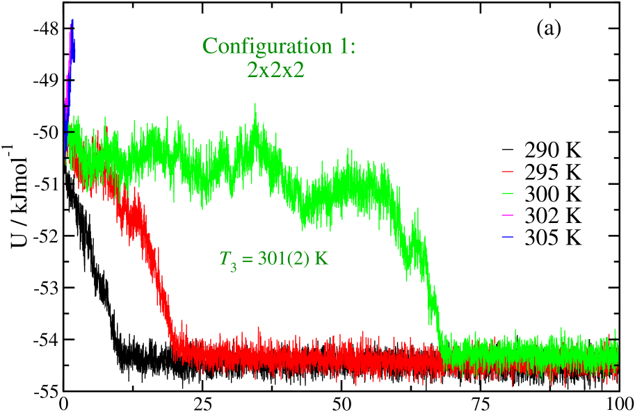
(a) Conf. 1

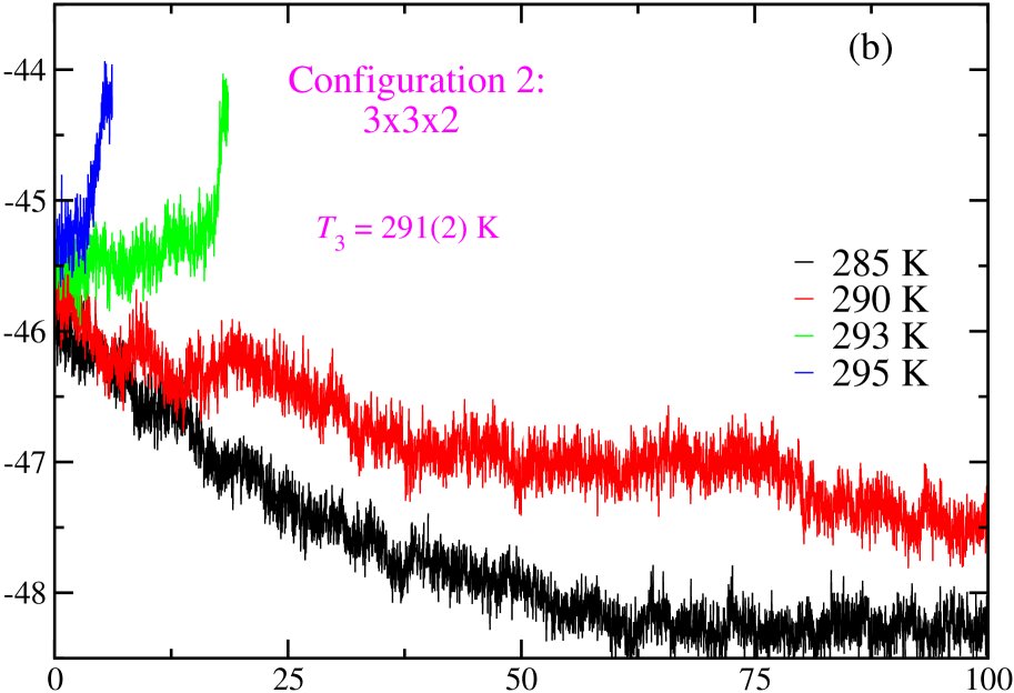
(b) Conf. 2

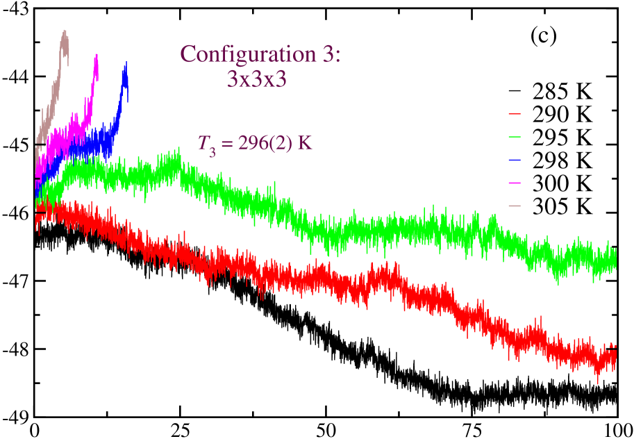
(c) Conf. 3

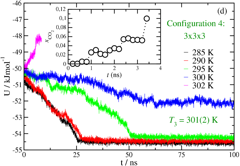
(d) Conf. 4

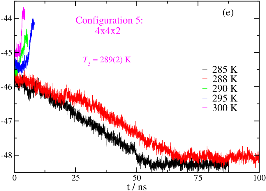
(e) Conf. 5

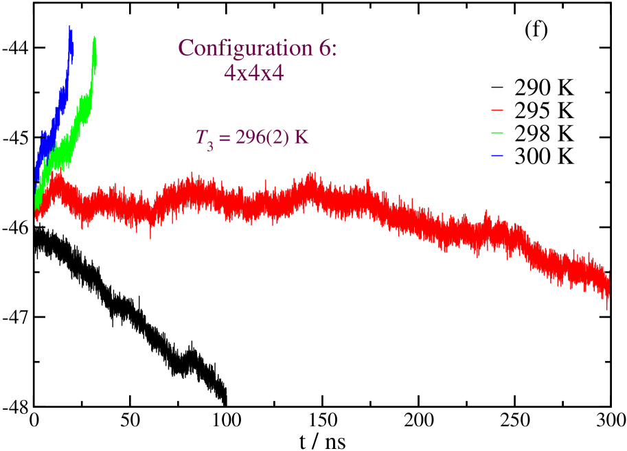
(f) Conf. 6

Figure 1: Evolution of the potential energy, as a function of time, for the 6 size-dependent configuration analyzed in the work. The results are obtained from MD-$NPT$ simulations at $2000\,\text{bar}$. Notice that panel (d) includes an inset with the molar fraction of CO₂ in the aqueous phase as a function of time at $285\,\text{K}.$

III.1 Effect of the stoichiometric configuration

We first consider two stoichiometric configurations, i.e., configurations in which the number of molecules of CO₂ and H₂O in the hydrate phases is the same as those in both liquid phases. The first configuration we analyze (configuration 1) is a system formed from 368 and 64 water and CO₂ molecules in the hydrate phase (all the cages of the hydrates are fully occupied, i.e., 8 CO₂ molecules per 46 water molecules in each unit cell in a $2\times 2\times 2$ sI structure) and the same number of molecules of each species in the liquid phases. According to the nomenclature used previously in paper I, Blazquez et al. (2024) this is a stoichiometric configuration. As we have already seen, it is important to compare the results obtained from simulations using stoichiometric systems with simulation data obtained using non-stoichiometric configurations. In this work, we compare the results with simulation data obtained by Míguez et al. Míguez et al. (2015) in which some of us estimated the three-phase coexistence temperature of the CO₂ hydrate using the same solid configuration ($2\times 2\times 2$) surrounded by liquid water (with the same number of water molecules) and a second liquid phase formed from $192$ CO₂ molecules, i.e., the triple number than that of the hydrate phase. This system is the configuration 0. According to the nomenclature used in this work, configuration 0 is not stoichiometric (see Table 1).

We have determined the three-phase coexistence temperature of configuration 1, $T_{3}$, in a wide range of pressures, from $100$ to $6000\,\text{bar}$, following the methodology already explained in paper I Blazquez et al. (2024) and in Section II. We first concentrate at a given pressure, $2000\,\text{bar}$, and then analyze the behavior of the system at different pressures. Fig. 1(a) shows the evolution of the potential energy of the system, $U$, as a function of time, at $2000\,\text{bar}$ and temperatures from $290$ to $305\,\text{K}$. As can be seen, two clear behaviors are observed. At the highest temperatures, $302$ and $305\,\text{K}$, the potential energy increases very quickly over time, indicating the melting of the CO₂ hydrate. Note that potential energy curves obtained at $302$ and $305\,\text{K}$ require very careful examination since the hydrate melts very quickly, in less than $3\,\text{ns}$, approximately. However, at low temperatures, $300$, $302$, and $305\,\text{K}$, the potential energy shows a sharp decrease, which is more pronounced as the temperature is lower, indicating that the hydrate solid phase grows. Since at $302\,\text{K}$ the potential energy increases and at $300\,\text{K}$, the potential energy decreases, the three-phase coexistence temperature at $2000\,\text{bar}$ is estimated at $T_{3}=301(2)\,\text{K}$. It is interesting to compare this prediction with the $T_{3}$ corresponding to the configuration 0 at the same pressure. According to Table 2, the $T_{3}$ obtained by Míguez et al. Míguez et al. (2015) was $292(2)\,\text{K}$. Based on this, the dissociation temperature of the stoichiometric configuration is $9\,\text{K}$ above that of the non-stoichiometric configuration of the liquid phases. This result is in agreement with our findings in paper I, Blazquez et al. (2024) indicating that the use of stoichiometric configurations produces an overestimation of the $T_{3}$.

Note that characteristic times at which the CO₂ hydrate crystallizes are shorter than those compared with the CH₄ hydrate. This is clearly seen comparing Figs. 1(a) of this work and Fig. 2a of paper I. Blazquez et al. (2024) In both cases, the system has exactly the same number of molecules in each phase. As can be seen, in the case of the CO₂, crystallization of the hydrate occurs relatively soon, between $10$ and $75\,\text{ns}$. However, the CH₄ hydrate needs even $200\,\text{ns}$ to crystallize if temperature is close of the $T_{3}$. This is an expected result since hydrate growth rate is controlled by mass transfer processes, which depends on the solubility and diffusivity of the guest molecules in water. Note that not only solubility but also diffusivity of CO₂ in water are one order of magnitude higher than those of CH₄ in water. Grabowska et al. (2022); Algaba et al. (2023a)

As we have previously mentioned, stoichiometric configurations simulated at temperatures below the $T_{3}$ of the hydrate, at the corresponding pressure, evolve into singular phases of hydrate. This is confirmed by the sharp decrease in the potential energy already shown in Fig. 1(a). As we will see later, this behavior indicates that the growing mechanism of the hydrate from these configurations is not only due to a layer-by-layer formation of the hydrate. In fact, as it happens with the CH₄ hydrate, Blazquez et al. (2024) this behavior confirms the presence, not of a bubble of CO₂ but a liquid drop of CO₂ within the liquid phase. Recall that CO₂ and water exhibit liquid-liquid immiscibility at the conditions at which the hydrate forms. Sloan and Koh (2008) This liquid drop collapses, at a certain time, producing a very quick formation of the hydrate phase corroborated by the abrupt decrease in the potential energy at this time. We have checked that the liquid drop mechanism is observed in the whole range of pressures considered in configuration 1. It is also important to remark on the quantitative difference found between the decrease of the potential energy of the CH₄ and CO₂ hydrates. In the first case, as can be seen in Fig. 2a of paper I, Blazquez et al. (2024) the sharp decrease is more pronounced than that compared with the CO₂ hydrate, as shown in Fig. 1(a) of this work. This indicates a quicker dissolution of the CH₄ bubbles than the CO₂ liquid drop. A more detailed account of the formation of the liquid drops in the CO₂ hydrate is presented below.

As we have already mentioned in paper I, Blazquez et al. (2024) this bubble formation has been previously observed by several authors. Walsh et al. Walsh et al. (2009, 2011) calculated nucleation rates after observing spontaneous nucleation of methane hydrate preceded by the formation of a bubble. In 2010, Conde and Vega Conde and Vega (2010) also observed bubble formation before hydrate growth when determining the $T_{3}$ of the methane hydrate. This bubble formation was also shown by Liang and Kusalik Liang and Kusalik (2011) for H₂S systems. After these pioneering studies, other works have studied the effect of bubble formation in the dissociation temperature of methane hydrates. Yagasaki et al. (2014); Grabowska et al. (2022); Fang et al. (2023); Bagherzadeh et al. (2015)

In paper I, we have concentrated on the estimation of the $T_{3}$ at a fixed pressure, $400\,\text{bar}$. In this work, we extend the study and consider the dissociation temperature of the CO₂ hydrate in a wide range of pressures. We have used the same procedure to evaluate the $T_{3}$ of the hydrate in a wide range of pressures, from $100$ to $6000\,\text{bar}$. At each pressure, we have simulated several temperatures, separated $5\,\text{K}$, from $280$ up to $310\,\text{K}$, approximately. The results obtained are presented in Table 2 (predictions obtained for the configuration 0 by Míguez et al. Míguez et al. (2015) are also included for comparison reasons).

To have an overall vision of the results obtained along the whole range of pressures, we have represented all the $T_{3}$ estimated in this work in a $PT$ or pressure-temperature projection, as shown in Fig. 2. Particularly, Fig. 2a shows the diagram corresponding to configuration 1. We have also included the simulation results of the configuration 0, studied by Míguez et al. Míguez et al. (2015) using a non-stoichiometric configuration (see Table 1 for further details). As can be seen, the main effect of using a stoichiometric instead of a non-stoichiometric configuration is to displace the whole dissociation line towards high temperatures. Particularly, the dissociation line of configuration 1 is located $9-14\,\text{K}$, depending on the pressure, above the dissociation line of configuration 0 (non-stoichiometric). Note that at $100\,\text{bar}$, differences between both $T_{3}$ values are $14\,\text{K}$. See the Table 2 for further details. Differences between the $T_{3}$ values of stoichiometric and non-stoichiometric ($2\times 2\times 2$) are much larger than in the case of the CH₄ hydrate. Blazquez et al. (2024)

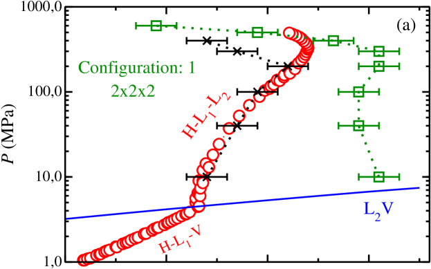
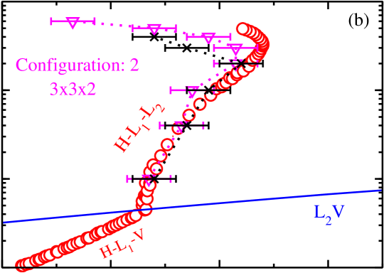
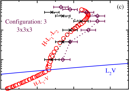
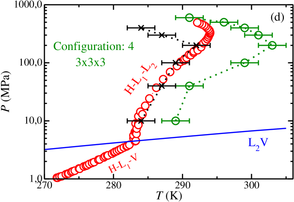
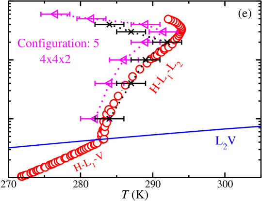
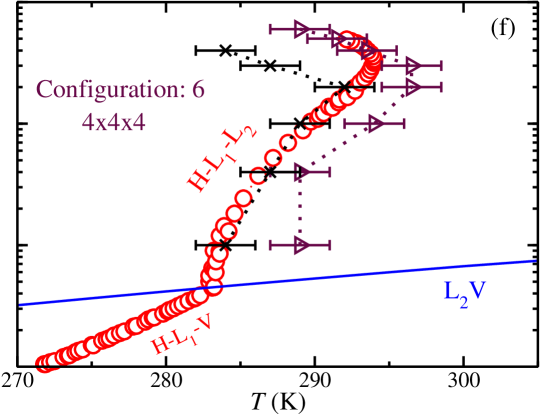
Figure 2: Pressure–temperature or $PT$ projection of the dissociation line of the CO₂ hydrate. The green squares (a), violet down triangles (b), maroon diamonds (c), green circles (d), violet left triangles (e), and maroon right triangles (f) represent the predictions obtained from simulation using the corresponding configuration. The red circles represent the experimental data taken from the literature Sloan and Koh (2008) and the blue curve is the experimental vapor pressure of the CO₂. Black crosses stand for the results obtained in the work of Míguez et al. Míguez et al. (2015)

We now study a second stoichiometric configuration but considering a larger system. In this case, we replicate the unit cell of the hydrate three times ($3\times 3\times 3$), instead of the two times of configuration 1 ($2\times 2\times 2$). According to this, the initial hydrate phase is now formed by $1242$ and $216$ water and CO₂ molecules, respectively. In order to have the same stoichiometry in the liquid phase, we surround the initial hydrate phase by a slab with $1242$ water molecules and a second slab with $216$ CO₂ molecules. This system corresponds to configuration 4 presented in Table 1, which is similar to configuration 6 presented in paper I for the CH₄ hydrate. Blazquez et al. (2024) It is interesting to compare the results obtained from this new stoichiometric configuration and check if the CO₂ hydrate shows the same general behavior.

Fig. 1(d) shows the evolution of the potential energy of configuration 4, as a function of time, at $2000\,\text{bar}$ and several temperatures, from $285$ to $302\,\text{K}$. As can be seen, there is an increase in the time needed to observe the crystallization or melting of the hydrate. It is worthy to mention that the time required to observe one of the behaviors is not so large as in the case of the CH₄ hydrate. This indicates again that CO₂ hydrates grow much quicker than CH₄ hydrates due to the high solubility of CO₂ in water. Blazquez et al. (2023) The dissociation temperature of the hydrate at $2000\,\text{bar}$ ranges between $302$ (the lowest temperature showing an increase in potential energy) and $300\,\text{K}$ (the highest temperature showing a decrease in potential energy). According to this, $T_{3}=301(2)\,\text{K}$. The corresponding dissociation temperature of configuration 0 (non-stoichiometric), at the same pressure ($2000\,\text{bar}$), is $292(2)\,\text{K}$. This is the same value obtained in the case of configuration 1. The potential energy curves, as functions of time for temperatures below the $T_{3}$, exhibit a similar behavior to those observed in configuration 1 (see Figs. 1(a) and 1(d)), with two minor differences: (1) the slope of the sharp decrease is now lower; and (2) the time required to observe the decrease is higher. The reason is due to the large size of configuration 4 compared with that of configuration 1 ($3.375$ times in terms of number of molecules). As we will see later, this also confirms the quick formation of liquid drops before the layer-by-layer growth of the hydrate at temperatures below the $T_{3}$.

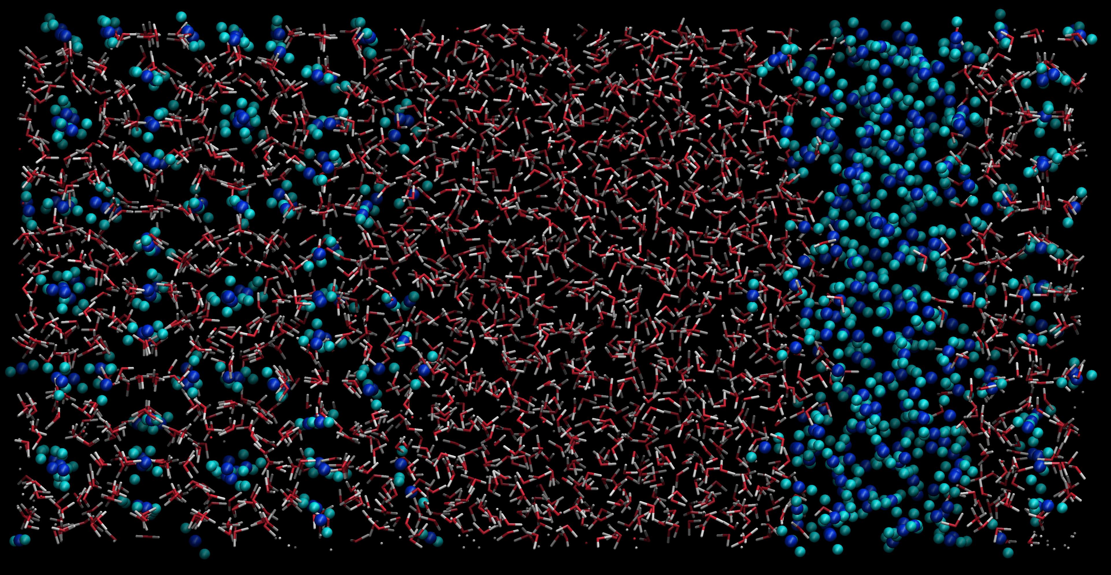
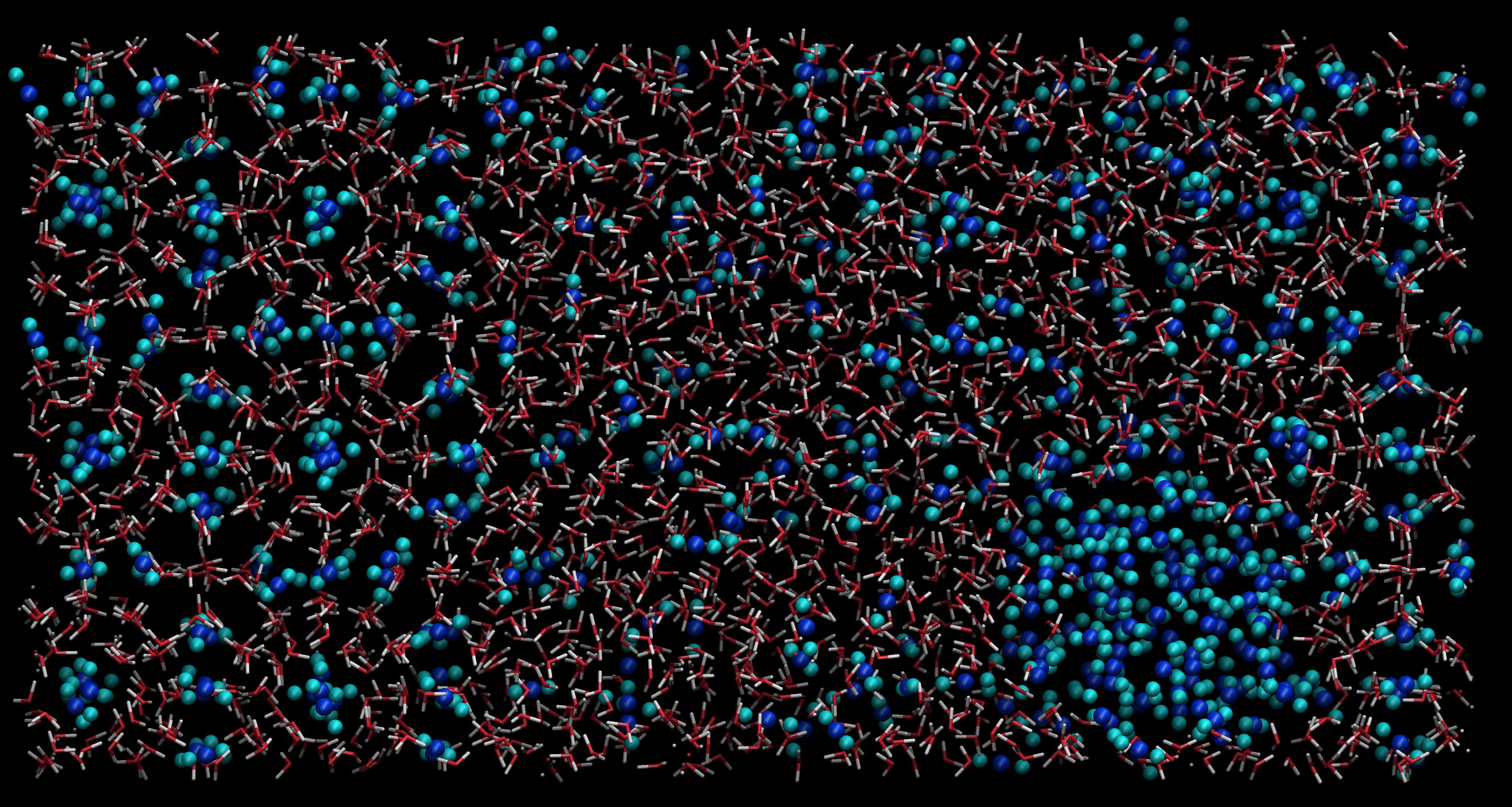
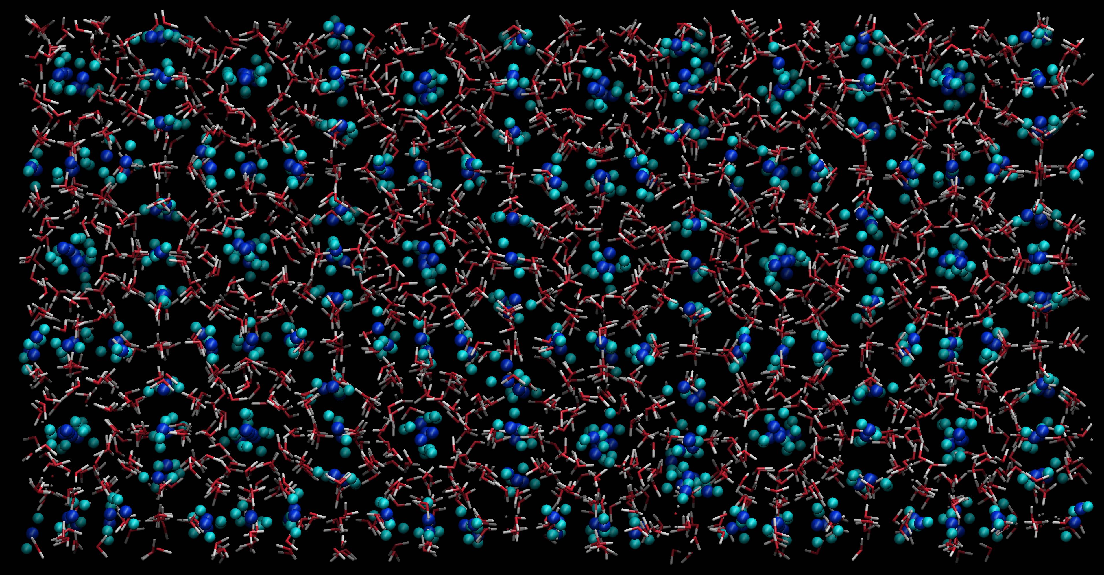
Figure 3: Snapshots taken at different times during $100\,\text{ns}$ simulation run for configuration 4 at 285 K and 2000 bar. The formation of a liquid drop and the growth of carbon dioxide hydrate are shown. From top to bottom: $t=0$ ns, three-phase initial configuration. $t=3$ ns, formation of a carbon dioxide drop within the liquid phase. $t=4$ ns, rupture of the carbon dioxide drop and the formation of an oversaturated solution. $t=25\,\text{ns}$, complete growth of the CO₂ hydrate. Water molecules are represented as white and red sticks and CO₂ molecules as cyan (carbon atom) and blue spheres (oxygen atoms).

The complete dissociation line of configuration 4 is also presented in Fig. 2d in a pressure-temperature projection of the phase diagram as in the previous case. We have also included the results corresponding to configuration 0 obtained by Míguez et al. Míguez et al. (2015). As it happens for configuration 1 (Fig. 2a), the dissociation line of configuration 4 is shifted towards higher temperatures at all pressures. However, the displacement is pressure-dependent if we compare it with the displacement observed in the case of configuration 1. Now, the shift is smaller at low pressures, similar at intermediate pressures, and larger at high pressures. This plot, with the results discussed in the previous paragraph, confirms that the liquid drop formation during the CO₂ hydrate growth is caused by the stoichiometric composition of the system, regardless of its size and the guest.

As in the case of the CH₄ hydrate study in our paper I, Blazquez et al. (2024) it is possible to observe the complete growth sequence of a liquid drop for configurations 1 and 4. Here we only show the formation of the CO₂ liquid drop in system 4, which corresponds to the initial $3\times 3\times 3$ configuration of the hydrate. It is important to mention that we have observed the same mechanism of formation of liquid drops, not only at all the pressures considered in this work ($100-6000\,\text{bar}$) for this configuration but also at all of the pressures for configuration 1 ($2\times 2\times 2$ system). The main difference between drops observed in configuration 1 is that they exhibit a smaller size compared with those formed in configuration $4$. As an example, Figure 3 shows four snapshots that illustrate the evolution of the configuration 4, at 2000 bar and 285 K. In the first snapshot (top), the initial hydrate phase is located on the left, with the pure water phase in the middle, and the CO₂ pure phase on the right ($0\,\text{ns}$). In the second snapshot (second panel from top), a liquid drop of CO₂ is formed within the water-rich liquid phase that can be clearly observed next to the water-CO₂ interface ($3\,\text{ns}$). It is interesting to compare this drop with the CH₄ bubble presented in paper I. Blazquez et al. (2024) In this case, the drop is more difficult to distinguish than in the methane case due to the high solubility of CO₂ in the water-rich liquid phase. Then, the liquid drop ruptures and supersaturated aqueous solution of CO₂ appears in the central region of the simulation box, as can be seen in the third snapshot from the top shown in Fig. 1(d) ($4\,\text{ns}$). Finally, the last snapshot (bottom) shows the complete formation of the hydrate phase ($25\,\text{ns}$). Notice that this time corresponds to the end of the slope shown in Fig. 1(d) when the complete growth of the hydrate occurs. As we have already mentioned, this is the expected behavior since configuration 4 corresponds to a stoichiometric system and the final state corresponds to a single hydrate phase.

In the supplementary material, we provide a movie of the simulation trajectory at $285\,\text{}K$ and $2000\,\text{K}$ for configuration 4. The movie illustrates the diffusion of CO₂ molecules from the CO₂-rich liquid phase to the aqueous phase and the formation of the droplet. It shows how the droplet gradually reduces in size (thus, growing the hydrate at the same time) until it ruptures, resulting in a supersaturated solution and the complete growth of the hydrate phase. The visualization of the trajectory reveals a curved interface between the CO₂ droplet and aqueous solution, contrasting with the planar interfaces observed in the rest of the phase coexistence in the system.

The mechanism of the formation of the bubble, in the case of the CH₄ hydrate, and the liquid drop, in the case of the CO₂ hydrate, is completely analogous. However, the time scales are very different. In the first case, the formation of the bubble corresponds to the exact moment when the potential energy starts to drop abruptly (see Fig. 2f of paper I). Contrary, in the second case (CO₂), the formation of the drop starts at $0.8\,\text{ns}$. Note that potential energy in this case starts to drop at the beginning of the simulation. In addition to this, the temporal sequence at which the bubble forms, it ruptures, and the solid phase occupies the whole simulation box in the case of the CH₄ hydrate is $415\,\text{ns}\rightarrow 440\,\text{ns}\rightarrow 500\,\text{ns}$, approximately. However, in the case of the CO₂ hydrate is really different: $3\,\text{ns}\rightarrow 4\,\text{ns}\rightarrow 25\,\text{ns}$, approximately. The reason for these differences has to be found in the high difference between the solubility of CO₂ and CH₄ in water: in this case, the high concentration of CO₂ in water acts as a driving force that enhances the diffusion of CO₂ molecules in the water-rich liquid phase, the formation of the liquid drop, and finally, the formation of the complete hydrate phase. To corroborate this point, we have also calculated the solubility of CO₂ in the aqueous phase as a function of time. As it happens in paper I, Blazquez et al. (2024) we observe a large increment of CO₂ concentration in the aqueous solution just at the beginning of the droplet formation. This can be clearly seen in the inset of Fig. 1(d). The same behavior has been previously observed by Kusalik and coworkers for other hydrates. Hall, Zhang, and Kusalik (2016)

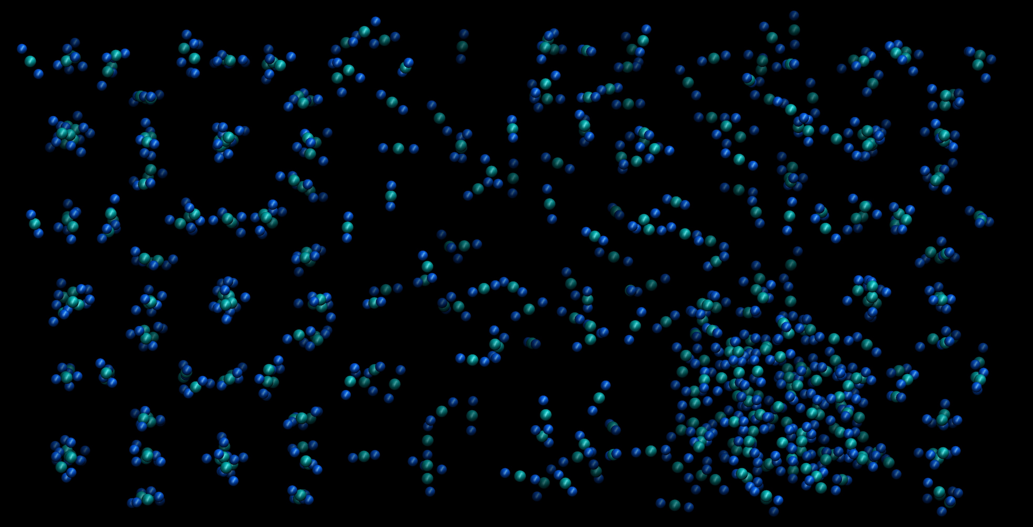
Figure 4: Snapshots of the $xz$ (top) and $yz$ (bottom) planes taken for configuration 4 at $285\,\text{K}$ and $2000\,\text{bar}$, showcasing the emergence of a CO₂ liquid drop within the liquid phase at $t=3\,\text{ns}$. For clarity, water molecules are omitted, while CO₂ molecules are represented as cyan (carbon atom) and blue spheres (oxygen atoms). CO₂ molecules are visible within the hydrates on the left and right sides of the figure. In the central region, CO₂ molecules are shown forming a cylindrical liquid drop.

As we have already mentioned, in paper I we have observed the formation of CH₄ bubbles for stoichiometric configurations of the hydrate. Blazquez et al. (2024) Particularly, we have discussed in detail not only the formation and stability of the CH₄ bubble, but also its shape. Simulation results of paper I demonstrate that the CH₄ bubbles exhibit a cylindrical shape instead of a spherical one. An obvious question arises in this context: are the CO₂ liquid drops observed in the current simulations spherical or cylindrical, as in the case of the CH₄ hydrate? To answer this question, we analyze the snapshot presented in Fig. 3b ($t=3\,\text{ns}$) corresponding to the simulation of configuration 4 at $285\,\text{K}$ and $2000\,\text{bar}$. It is important to recall again that we have observed the formation of liquid drops of CO₂, not only at this particular pressure but in the whole range of pressures along the dissociation line of the hydrate. Particularly, we have also observed the drops in configuration 1 ($2\times 2\times 2$). However, since the solubility of CO₂ in water is high ($10$ times higher than that of CH₄ in water, approximately), it is more difficult to distinguish the drops. For this reason, we concentrate here on liquid drops of configuration 4.

Fig. 4 shows the projection of the $xz$ plan (top), as well as the $yz$ projection (bottom) of the same configuration. To help the visualization of the drop we have omitted the water molecules. As can be seen, the second projection ($yz$) clearly shows that the liquid drop extends along the whole $y$-axis of the simulation box. As it discussed in paper I, Blazquez et al. (2024) and according to the Laplace equation, cylindrical interfaces result in lower solubility than spherical ones but higher than planar interfaces. If the liquid drops were stable and sufficiently large, the dissociation temperature would be shifted towards higher temperatures compared with the planar interface. In this work, as in paper I, drops of CO₂ are only stable for $1-20\,\text{ns}$, even less than in the case of the CH₄ bubbles ($10-25\,\text{ns}$).

As we have mentioned in the previous paragraph, the enhanced solubility of CO₂ in the aqueous phase in the presence of droplets compared to a planar interface at constant temperature can be understood in the context of the Laplace equation. According to this, the pressure inside the cylindrical droplets exceeds $2000\,\text{bar}$ (the outside pressure of the system). This higher internal pressure yields a higher chemical potential, leading to a higher molar fraction assuming ideal behavior for CO₂ in water. This excess of pressure can be estimated following our previous work. Grabowska et al. (2022) Here, we use the Laplace equation for droplets with cylindrical geometry ($\Delta P=\gamma/R$) to estimate the pressure inside the droplet. Here $\Delta P$ is the difference of pressure inside and outside the cylindrical drop, $\gamma$ is the water-CO₂ interfacial tension, and $R$ is the radius of the cylinder. To this end, we have calculated the aqueous solution - CO₂-rich liquid-liquid interfacial free energy using the same procedure as in our previous work. Algaba et al. (2023a) The interfacial tension at $2000\,\text{bar}$ and $285\,\text{K}$ is $\gamma=30.2(3)\,\text{mJ/m}^{2}$. We have also calculated the radius for the observed droplet at the same thermodynamic conditions. In this case, $R=0.76(10)\,\text{nm}$, approximately. Using the Laplace equation, the internal pressure is about $2400(50)\,\text{bar}$. As expected, this pressure is higher than the $2000\,\text{bar}$ of the global system, leading to higher solubilities of CO₂.

In summary, as it happens in the case of the CH₄ hydrate, the presence of liquid drops of CO₂ modifies the prediction of the $T_{3}$ of CO₂ hydrates. This is only observed in liquid configurations that have stoichiometric configurations, such as configurations 1 and 4 studied in this work. Hence, we do not recommend the use of stoichiometric configurations in order to get reliable predictions of the $T_{3}$ of CO₂ hydrates. Particularly, the recommendation for future studies is to use the configuration $3$ ($3\times 3\times 3$), which is non-stoichiometric, formed from an appropriate number of water and CO₂ molecules that allow to simulate the system in a reasonable time. It is worth mentioning, as it happens with bubbles in the case of the methane hydrate studied in paper I, Blazquez et al. (2024) that the formation of the droplets is expected not only in systems with stoichiometric compositions (i.e., when the ratio of molecules of CO₂ in the CO₂-rich liquid phase to that of water in the liquid phase is 8/46 , i.e., 0.174) but also in systems with lower values of this ratio. In fact, in these cases, the formation of the droplet is expected to occur at shorter times.

The formation of droplets should be directly related with the thickness of the CO₂-rich liquid phase in contact with the aqueous solution. To identify if there exists a critical thickness below which droplet formation is expected, we have simulated a water - CO₂ planar interface, without hydrate phase, using the direct coexistence simulation technique. Particularly, we use 1242 water molecules with a CO₂ liquid phase with different numbers of CO₂ molecules (i.e., $648$, $500$, $450$, $400$, and $350$). Simulations are performed using the anisotropic isothermal-isobaric or $NP_{z}\mathcal{A}T$ ensemble, with a fixed interfacial area of the systems of $3.6\times 3.6=12.96\,\text{nm}^{2}$, at $2000\,\text{bar}$ and $290\,\text{K}$. In all cases, simulations are run during at least $60\,\text{ns}$. We observe the formation of the droplets only in the systems formed from $400$ CO₂ molecules or less. According to this, our estimation of the critical thickness of the CO₂ slab is about 1.53-1.58 nm, approximately. In other words, when the thickness of the CO₂ phase is larger than $1.58\,\text{nm}$ no droplet is formed in $60\,\text{ns}$.

In any case, further work is needed to determine precisely under which conditions the planar water-CO₂ interface is not stable with respect to the formation of a cylindrical or spherical droplets as has been done for one component systems in other studies. MacDowell, Shen, and Errington (2006); Singh et al. (2019); Montero de Hijes and Vega (2022) In fact, in the future, it would also be interesting to study the droplet shape in bigger systems, as we have also stated in paper I. Blazquez et al. (2024)

Before finishing this section, it is important to briefly mention how simulation results obtained from stoichiometric configurations 1 and 4 compare with experimental data taken from the literature. As can be seen in Figs. 2a and 2d, simulation predictions exhibit large deviations with respect to experimental data. This is expected since, according to our previous discussion, the use of these kinds of configurations produces an overestimation of the $T_{3}$ at all the pressures along the dissociation line of the hydrate. We shall discuss in detail this issue in the last section, where we present the finite-size effect of non-stoichiometric configuration on the T₃ along the dissociation line of the CO₂ hydrate.

III.2 Effect of the overall size

Once we have analyzed in detail the effect of using two different stoichiometric configurations to determine the dissociation temperature of the CO₂ hydrate in a wide range of pressures, we now turn on to study the finite-size effects on $T_{3}$ for non-stoichiometric configurations. In this first section, we concentrate on finite-size effects due to the same increase in the number of molecules in each of the phases involved.

The control configuration used in this section is again configuration 0, with $992$ total number of molecules, and an initial configuration formed from $432$ ($368+64$) water and CO₂ molecules in the hydrate phase, $368$ water molecules in the water phase, and $192$ CO₂ molecules in the CO₂-rich liquid phase. Note that the non-stoichiometric composition of the liquid phases is verified since the number of CO₂ molecules in that phase is three times the number corresponding to the stoichiometric composition ($192=3\times 64$). Note that the size of the interfacial area and the length of the simulation box perpendicularly to the interface also increase. We first determine the dissociation temperatures, in the whole range of pressures already considered in the previous section, of configuration 3. According to Table 1, this configuration contains a total number of molecules equal to $3348$. This means that the system size, in terms of the number of molecules, is multiplied by a factor of $3.375$, keeping the non-stoichiometric composition of the liquid phases. As can be seen in Table 1, the number of molecules of each species is multiplied by this factor in each of the phases forming the initial simulation box of configuration 3.

We have determined the three-phase coexistence temperature of configuration 3, in the same range of pressures considered previously (from $100$ to $6000\,\text{bar}$). Fig. 1(c) shows the evolution of the potential energy of the system, $U$, as a function of time, at $2000\,\text{bar}$ and temperatures from $285$ to $305\,\text{K}$. As in the case of the stoichiometric configurations, we observe the same two behaviors: at the highest temperatures, $298$, $300$, and $305\,\text{K}$, the potential energy increases very quickly over time, indicating the melting of the CO₂ hydrate. However, at low temperatures, $295$, $290$, and $285\,\text{K}$, the potential energy shows a decrease, which is more pronounced as the temperature is lower, indicating that the hydrate solid phase is growing. The three-phase coexistence temperature at $2000\,\text{bar}$ is estimated at $T_{3}=296(2)\,\text{K}$ (at $298\,\text{K}$ the potential energy increases and at $295\,\text{K}$, it decreases).

It is interesting to compare the evolution of the potential energy obtained in this configuration and those corresponding to the stoichiometric configurations, 1 and 4. Although system sizes are different, it is clear that the characteristics sharp decreases observed in Figs. 1(a) and 1(d) are not seen in Fig. 1(c). The reason, as clearly stated in paper I, Blazquez et al. (2024) is that configuration 3 is not stoichiometric. According to this, the $T_{3}$ value corresponding to this configuration is reliable and can be compared with confidence with that obtained by Míguez et al. Míguez et al. (2015) for configuration 0. According to Table 2, the T₃ at $2000\,\text{bar}$ was $292(2)\,\text{K}$ (configuration 0). In other words, the dissociation temperature of the configuration 3 is $4\,\text{K}$ above that of the configuration 0. This result suggests that there is a finite-size effect on $T_{3}$ that displaces the dissociation temperature towards higher temperatures, making the hydrate phase more stable at this pressure.

To confirm the stabilization of the hydrate when the number of molecules considered in the simulation box is increased (by a factor of $3.375$), we have determined the $T_{3}$ at the whole range of pressures, from $100$ to $6000\,\text{bar}$. Results are presented in Fig. 2c. As can be seen, the dissociation line corresponding to configuration 3 (maroon diamonds) is systematically displaced with respect to the results obtained from configuration 0 (black crosses). Simulation data obtained from MD-$NPT$ simulations is also included in Table 2. Displacement is not homogeneous. At low pressures (below $400\,\text{bar}$), the T₃ increases $\sim 2\,\text{K}$, resulting in good agreement with previous results within the error bars. However, as the pressure is increased, displacement increases $~{}\sim 4-5\,\text{K}$ at intermediate pressures ($1000$ and $2000\,\text{bar}$. Finally, at the highest pressures ($\geq 3000\,\text{bar}$), the T₃ is shifted $7-9\,\text{K}$.

To better understand the finite-size effect on the location of the dissociation line of the CO₂ hydrate, we go further and consider a new larger system. Configuration 6 is formed by a total number of molecules equal to $7936$, $3456$ corresponding to the (stoichiometric) hydrate phase, and $4480$ molecules to the non-stoichiometric liquid phases. Note that now, the total number of molecules in configuration 6 is $8$ times larger than in configuration 0. Details of the particular number of water and CO₂ molecules can be inspected in Table 1. As in the previous cases, we first concentrate on the determination of the T₃ at an intermediate pressure, $2000\,\text{bar}$. As can be seen in Fig. 1(f), the system melts at the two highest temperatures considered, $298$ and $300\,\text{K}$, and freezes at $295$ and $290\,\text{K}$. According to this, the $T_{3}$, at $2000\,\text{bar}$, is $296(2)\,\text{K}$. Similarly to what happens with the previous non-stoichiometric configuration 3 (Fig. 1(c)), the evolution of the potential energy, as a function of time, behaves without the characteristic sharp drop associated with configuration 1 and 4 shown in Figs. 1(a) and 1(d). Note that now, the time required to observe crystallization is much larger than in smaller systems: in configuration 3, we observe crystallization before $100\,\text{ns}$. However, in configuration 6 we see that at temperatures close to the $T_{3}$, i.e., $295\,\text{K}$, crystallization occurs for times higher than $300\,\text{ns}$.

According to the results discussed in the previous paragraph, the $T_{3}$ predicted in configurations 3 and 6 are equal, $296(2)\,\text{K}$. Taking into account the results obtained for the CH₄ hydrate in paper I, Blazquez et al. (2024), an obvious question arises: is it necessary to simulate systems as large as the configuration 6 to predict $T_{3}$ values without finite-size effects? To answer this question, we have obtained the rest of the dissociation temperatures at different pressures. The results are presented in Fig. 2f. As can be seen, there is a similar shift of the dissociation line of configuration 6 (maroon right triangles) with respect to that of configuration 0 (black crosses) in Figs. 2c and 2f, indicating that we have achieved an asymptotic limit. A careful inspection of Table 2 confirms this hypothesis: except for the $T_{3}$ value at $100\,\text{bar}$, the $T_{3}$ values of configurations 3 and 6 are identical (within the error bars). In summary, configurations 3 and 6, formed from the larger unit cells (e.g., $3\times 3\times 3$ and $4\times 4\times 4$) show convergence of the $T_{3}$ values. This suggests that no finite-size effects exist for these system sizes.

III.3 Effect of size of the interfacial area

In the previous section, we have analyzed the finite-size effects of non-stoichiometric configurations on the dissociation line of the CO₂ hydrate varying the number of molecules in the system isotropically, i.e., increasing the initial hydrate phase in the three directions ($2\times 2\times 2$, $3\times 3\times 3$, and $4\times 4\times 4$). In addition to this, we consider the same number of water molecules in the aqueous phase and with three times more molecules of CO₂ in the CO₂-rich liquid phase to avoid stoichiometric configurations in the liquid phases. We have demonstrated that there exist finite-size effects associated with these changes.

We now investigate if the size of the interfacial area of the simulation box affects the $T_{3}$ of the CO₂ hydrate. To this end, we proceed similarly but considering two configurations in which the initial hydrate phases are formed replicating the unit cell as $3\times 3\times 2$ (configuration 2) and $4\times 4\times 2$ (configuration 5). The corresponding liquid phases are formed from the same number of water molecules in the aqueous phase as in the hydrate and with the number of CO₂ molecules equal to three times those existing in the hydrate. The particular number of molecules in each configuration can be seen in Table 1. Note that the total number of molecules in configurations 2 and 5 are $2232$ and $3969$, respectively.

Figs. 1(b) and 1(e) show the evolution of the potential energy of configurations 2 and 5, as functions of time, at $2000\,\text{bar}$, respectively. The same general trend is observed in both figures, similar to those presented by configurations 3 and 6 (Fig. 1(c) and 1(f)), i.e., since both configurations are non-stoichiometric they do not show the sharp decrease in potential energy. Following the same procedure used in previous sections, $T_{3}$ of both configurations can be easily determined by inspecting the behavior of potential energy at different temperatures. The $T_{3}$ values predicted by the molecular models are $291(2)$ and $289(2)\,\text{K}$ for configurations 2 and 5, respectively. These results suggest that the $T_{3}$ values of both configurations are equal (within the error bars) and also equal to the $T_{3}$ value corresponding to the configuration 0 ($2\times 2\times 2$) at this pressure. This is a non-expected result according to the behavior observed in the previous section, especially if we take into account that configuration 5 is formed from $3968$ molecules, a $20\%$ more molecules than in configuration 3 ($3\times 3\times 3$). For this former configuration, $T_{3}$ is equal to $296(2)\,\text{K}$ at the same pressure.

To clarify this point, we have also obtained the $T_{3}$ values of configurations 2 and 5 at lower and higher pressures, as we have already done with the configurations previously studied. Fig. 2c and 2f show the pressure-temperature projection of the dissociation line of the CO₂ hydrate using both configurations. The numerical data obtained from MD-$NPT$ simulations are also presented in Table 2. As can be seen in the plots, both configurations exhibit very similar $T_{3}$ values in the whole range of pressures. Particularly, at low pressures, between $100$ and $2000\,\text{bar}$, configurations 0 (black crosses) and 2 (violet down triangles) present the same $T_{3}$ values, while configuration 5 (violet left triangles) seem to exhibit slightly lower values of $T_{3}$. However, both results are within the error bars. At higher pressure, above $3000\,\text{bar}$, the dissociation temperatures of configurations 2 and 5 are above those of configuration 0. Nevertheless, the results are again within the error bars and no significant differences are observed between temperatures at the corresponding pressure (see Table 2 for further details).

In summary, we have analyzed the finite-size effects on the $T_{3}$ for configurations 2 ($3\times 3\times 2$) and 5 ($4\times 4\times 2$). The main difference between these two configurations is that configuration 5 has a larger interfacial area in contact with the aqueous and CO₂-rich liquid phases ($4\times 4$ unit cells) than that of configuration 2 ($3\times 3$ unit cells). Results indicate that finite-size effects on $T_{3}$ values are negligible, at least within error bars.

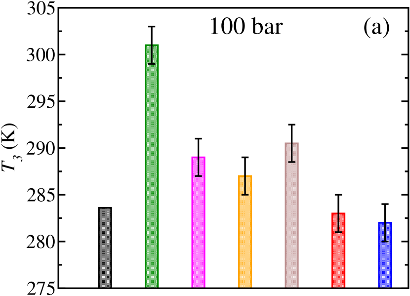
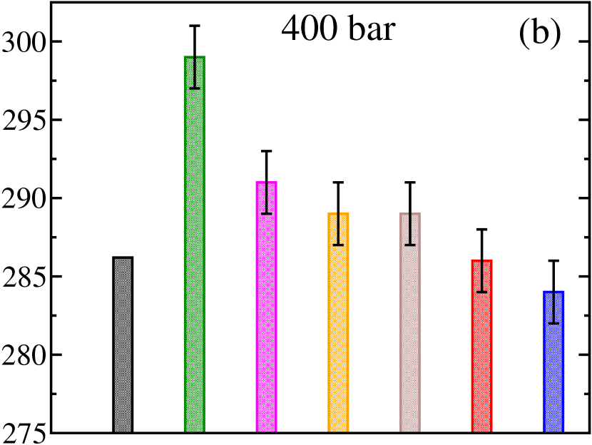
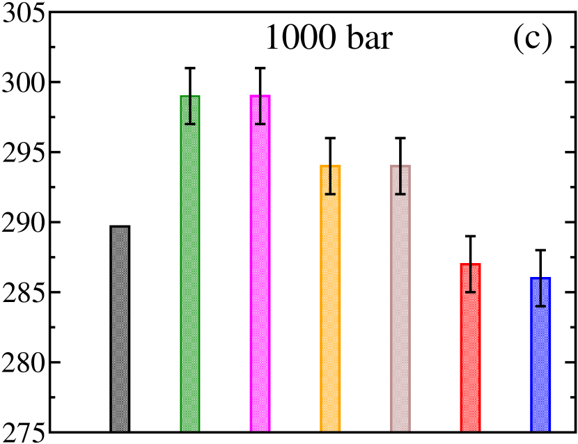
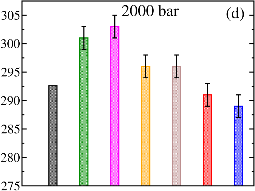
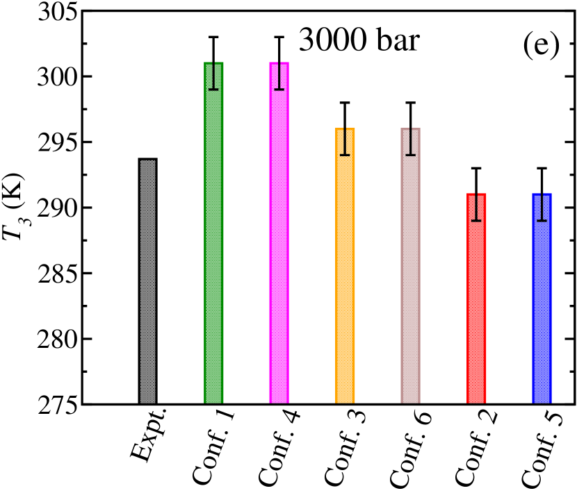
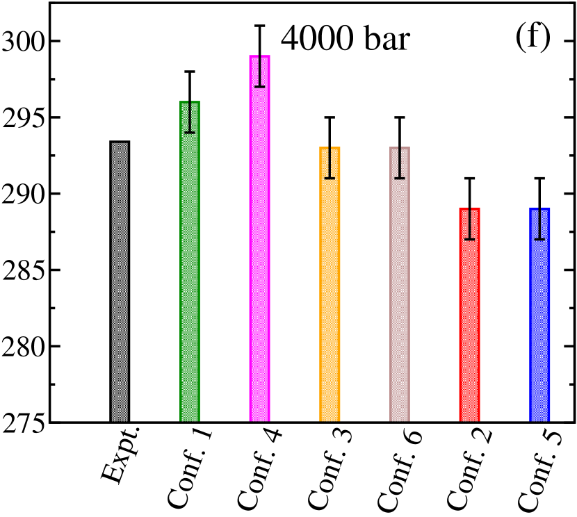
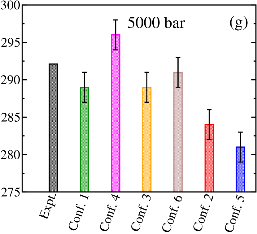
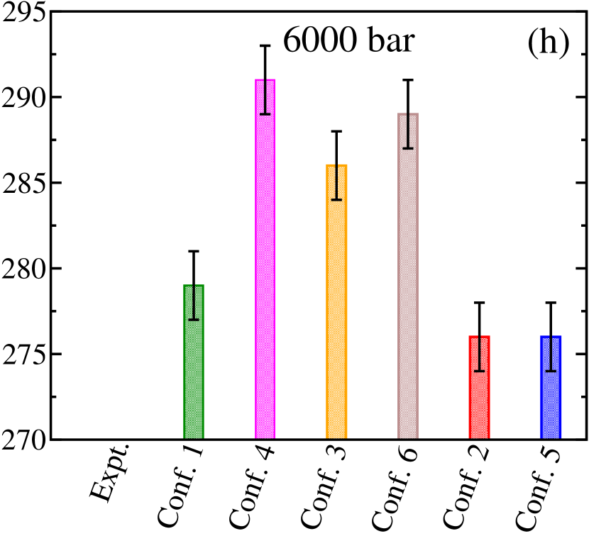
Figure 5: Comparison of the three-phase coexistence temperatures ($T_{3}$) for the CO₂ hydrate from the 6 size-dependent configurations analyzed in this work at several pressures. The experimental $T_{3}$ values taken from the literature, Sloan and Koh (2008) at different pressures, are also included. In all cases, the composition of the initial configuration is analogous, formed by a CO₂ hydrate phase in coexistence with a liquid water phase and a CO₂ liquid phase with the corresponding numbers of molecules in each configuration.

III.4 Effect of hydrate thickness

We have already discussed in Section III.C the effect of passing from the configuration 0 ($2\times 2\times 2$) to systems with configurations 2 ($3\times 3\times 2$) and 5 ($4\times 4\times 2$). In both cases, we have analyzed the effect of increasing the interfacial area keeping invariant the thickness of the hydrate along the $z$-direction (perpendicular to the solid-fluid interface). But there is also an interesting comparison not made until now: the effect of increasing the thickness of the hydrate along the $z$-direction keeping constant the interfacial area. This can be done by comparing configurations 2 ($3\times 3\times 2$) and 3 ($3\times 3\times 3$), in which the thickness of the hydrate passes from $2$ to $3$ unit cells along the $z$-direction, and configuration 5 ($4\times 4\times 2$) and 6 ($4\times 4\times 4$). In the first case the interfacial area is $3\times 3$ unit cells and in the second case $4\times 4$. Note that in both comparisons the interfacial area remains unchanged.

We first consider the comparison between configurations 2 and 3 at $2000\,\text{bar}$. Following the same procedure used in previous cases (inspection of Figs. 1(b) and 1(c)), the dissociation temperature predicted from both configurations are $291(2)$ and $296(2)\,\text{K}$, respectively. These results confirm that an increase in the thickness of the hydrate in the initial simulation box helps to stabilize the system. We have also investigated the same behavior at lower and higher temperatures. This information can be readily obtained from inspection of Figs. 2b and 2c. The numerical results obtained from MD-NPT simulations are also presented in Table 2. As can be seen, the main effect of increasing the thickness of the hydrate phase is to shift the $T_{3}$ towards higher temperatures at all pressures. The displacement of the three-phase line is not uniform but varies as the pressure increases: $3-4\,\text{K}$ at low pressures ($100$ and $200\,\text{bar}$), $4-7\,\text{K}$ at intermediate pressures ($1000-4000\,\text{bar}$), and $5-10\,\text{K}$ at high pressures ($5000$ and $6000\,\text{bar}$).

We have also analyzed the changes observed when passing from configuration 5 ($4\times 4\times 2$) to configuration 6 ($4\times 4\times 4$). Note that in this case, the interfacial area is $4\times 4$ instead of $3\times 3$ units cells. In addition to that, the increase of the hydrate thickness varies from $2$ to $4$ hydrate unit cells along the $z$-direction (perpendicular to the interface). As can be seen in Figs. 2e and 2f, the effect of increasing the hydrate thickness is also to shift the $T_{3}$ values toward higher temperatures. In this case, the increase of the stability of the hydrate is higher than in the previous case. Particularly, $5-7\,\text{K}$ at low pressures ($100$ and $200\,\text{bar}$), $4-8\,\text{K}$ at intermediate pressures ($1000-4000\,\text{bar}$), and $10-15\,\text{K}$ at high pressures ($5000$ and $6000\,\text{bar}$).

To recap, the main effect of increasing the hydrate thickness is to shift the dissociation line towards higher temperatures as the hydrate thickness increases, i.e., to increase the stability of the hydrate phase.

III.5 Comparison with experimental data

In the previous sections, we discuss the finite-size effects on the $T_{3}$ of the CO₂ hydrate in a wide range of pressures. This is performed using 6 different configurations and comparing the results with the configuration 0 obtained several years ago by Míguez et al. Míguez et al. (2015) In this Section, we focus on the comparison of the predictions obtained using these configurations with experimental data taken from the literature.

In the original work, Míguez et al. (2015) the authors proposed a modified Berthelot combining rule that allows to predict the dissociation line of the CO₂ hydrate in a wide range of pressures with confidence. Particularly, differences between predictions obtained from configuration 0 and experimental data taken from the literature Sloan and Koh (2008) are below $1\,\text{K}$ from $100$ to $2000\,\text{K}$. At high pressures, at $3000\,\text{bar}$ and above, agreement between both results deteriorates. Although the model is able to capture the existence of the reentrant behavior of the dissociation line, the agreement is only qualitative. We recommend the reader to the original paper for a detailed account of this issue. Míguez et al. (2015)

Fig. 2 shows the pressure-temperature composition of the dissociation line of the CO₂ hydrate as predicted from the model proposed by Míguez et al. Míguez et al. (2015) using the 6 configurations considered in this work. The results obtained using configuration 0 are also presented, as well as the experimental data taken from the literature. Sloan and Koh (2008) We only analyze the agreement between experimental data and predictions obtained using non-stoichiometric configurations (2, 3, 5, and 6) since stoichiometric systems do not provide the correct $T_{3}$ due to the presence of CO₂ liquid drops discussed in Section III. A. Let’s concentrate on predictions obtained using configurations 3 and 6. As can be seen, predictions from configuration 3 overestimate the experimental $T_{3}$ in the whole range of pressures. Particularly, $T_{3}$ is overestimated $\sim 5\,\text{K}$ at low pressures, below $3000\,\text{bar}$. The agreement between predictions from configuration 6 and experimental data is similar.

The main conclusion is that finite-size effects also affect agreement with experimental data. What is the reason for this? The answer is simple. The unlike interaction parameter associated with the Berthelot rule, $\xi$, was established by Míguez et al. Míguez et al. (2015) using configuration 0, i.e., using a $2\times 2\times 2$ configuration and a certain cutoff distance for the dispersive interactions. We will not discuss here the effect of the cutoff distance on the $T_{3}$ of hydrates. We recommend to read the paper III of this series in which we analyze the effect of the dispersive interactions on the three-phase equilibria of CH₄ and CO₂ hydrates. Algaba et al. (2023b) According to this, the value $\xi=1.13$ obtained by Míguez et al. Míguez et al. (2015) allows to quantitatively predict the dissociation line of the CO₂ hydrate for the particular configuration ($2\times 2\times 2$) used to fit experimental data. As we have demonstrated in Section III. B, the use of larger configurations, i.e., configurations 3 and 6, produces a displacement of the dissociation line of the CO₂ towards higher temperatures, making the hydrate phase more stable. In fact, the same effect produces the use of a positive modification of the Berthelot rule ($\xi>1$). This suggests that the $\xi=1.13$ value is too high for describing in a quantitative way the dissociation line of the CO₂ hydrate using configurations not affected by finite-size effects, i.e., configurations 3 or 6.

Finally, we have summarized the $T_{3}$ values obtained for each of the 6 size-dependent configurations, at all the pressure considered (from $100$ to $6000\,\text{bar}$), in the bar graphs of Fig. 5. In addition, we have also included the experimental $T_{3}$ for comparison reasons (first column). The order of the columns, from left to right, takes into account the effect of the stoichiometric configurations (1 and 4), of the overall size of the system (3 and 6), and of the size of the interfacial area (2 and 5). The first configurations in each of the three groups, 1, 2, and 3, correspond to the smaller system analyzed, and the second ones, 4, 5 and 6, to the larger systems. See Table 1 for further details. As can be seen, the main conclusions stated in the previous sections can be observed in Fig. 5 in the whole range of pressures analyed in this work: (1) overestimation of the T₃ values, with respect to the experimental data taken from the literature, in the case of the stoichiometric configurations (1 and 4); (2) similar $T_{3}$ values for configurations 3 ($3\times 3\times 3$) and 6 ($3\times 3\times 3$); and (3) configurations 2 and 5 exhibit the same $T_{3}$ values at all pressures (within the error bars) but below the experimental T₃ values.

IV Concluding remarks

In this second part of a three-paper series dedicated to investigating finite-size effects in methane and carbon dioxide, as well as the influence of dispersive interactions on both hydrates, our focus is on the CO₂ hydrate. Specifically, we delve into the finite-size effects affecting the determination of the three-phase coexistence temperature ($T_{3}$) for CO₂ hydrate, employing molecular dynamics simulations in conjunction with the direct coexistence technique. Adhering to the methodology outlined in the first paper Blazquez et al. (2024), we examine six size-dependent configurations using realistic water and CO₂ models (i.e., TIP4P/Ice and TraPPE) to assess the impact of size and composition on the estimation of $T_{3}$. Given the similarity of our findings to those in the first paper Blazquez et al. (2024), we provide a concise summary of the most pertinent results:

• The simulation results obtained for the CO₂ hydrate confirm the sensitivity of $T_{3}$ depending on the size and composition of the system, explaining the discrepancies observed in the original work by Míguez et al. Míguez et al. (2015) in 2015. This is in agreement with the findings of paper I, Blazquez et al. (2024) not only at a particular pressure but in a wide range of pressures considered.

• Configurations with stoichiometric composition or less CO₂ molecules than the stoichiometric, at temperatures below $T_{3}$, evolve into a singular phase of CO₂ hydrate growth, as in the case of the methane hydrate. Blazquez et al. (2024) This is confirmed in the whole dissociation line, from $100$ to $6000\,\text{bar}$. In this case, there is no a bubble of methane but a liquid drop of CO₂. The mechanism of growing is via the emergence of a liquid drop of CO₂ within the liquid and the subsequent formation of an oversaturated CO₂ solution in water. Conversely, an excess of molecules in the CO₂-rich liquid phase in the initial configuration leads to the coexistence of CO₂ hydrate and CO₂ liquid phases without the formation of drops.

• Finite-size effects are pronounced in small systems with stoichiometric composition (e.g., configuration 1 with a unit cell of $2\times 2\times 2$), resulting in an overestimation of $T_{3}$ due to liquid drop formation during hydrate growth, causing a false stability of CO₂ hydrate by increasing CO₂ solubility. Note that this is a common conclusion in both methane and carbon dioxide hydrates.

• Non-stoichiometric configurations with larger unit cells, like $3\times 3\times 3$ and $4\times 4\times 4$, show convergence of $T_{3}$ values, suggesting that finite-size effects for these system sizes, regardless of drop formation, can be safely neglected.

• To study the T₃ of the CO₂ hydrate the best choice is configuration 3, which provides an accurate $T_{3}$ value, and affordable simulation times.

The primary outcome of this study, entirely consistent with the findings in the initial paper of this series for CH₄ hydrate Blazquez et al. (2024), can be succinctly summarized as follows: when using the direct coexistence technique to estimate the $T_{3}$ of CO₂ hydrate, it is crucial to avoid small stoichiometric configurations such as configuration 1. These configurations tend to develop drops at the onset of the run, leading to an overestimation of the $T_{3}$ value. The recommended and optimal choice is configuration 3, which provides an accurate $T_{3}$ value, and the computational resources required for simulating this system are currently feasible.

This study, complementing the initial paper in the series Blazquez et al. (2024), presents valuable insights into the finite-size effects observed in simulations of CO₂ hydrate. The findings highlight the possibility of mitigating finite-size effects in estimating $T_{3}$ by thoughtfully selecting system configurations. We anticipate that these results will contribute to a better understanding of finite size effects in the determination of $T_{3}$ for methane hydrates, addressing discrepancies in the existing literature and assisting researchers in selecting appropriate system sizes for future investigations. Our future research will delve into examining the potential impact of cutoff values and guest types on $T_{3}$ values, exploring how these factors are influenced by finite-size effects.

Supplementary material

See the supplementary material for the movie of the simulation trajectory at $285\,\text{K}$ and $2000\,\text{bar}$ for configuration $4$. The movie illustrates the CO₂ molecules diffusion from the CO₂-rich liquid phase to the aqueous phase and the formation of the droplet.

AUTHORS DECLARATIONS

Conflicts of interest

The authors have no conflicts to disclose.

Data availability

The data that support the findings of this study are available within the article.

REFERENCES

REFERENCES

- Sloan (2003) E. D. Sloan, “Fundamental principles and applications of natural gas hydrates,” Science 426, 353–359 (2003).
- Koh, Sum, and Sloan (2012) C. A. Koh, A. K. Sum, and E. D. Sloan, “State of the art: Natural gas hydrates as a natural resource,” J. Nat. Gas Sci. Eng. 8, 132–138 (2012).
- Sloan and Koh (2008) E. D. Sloan and C. Koh, Clathrate Hydrates of Natural Gases, 3rd ed. (CRC Press, New York, 2008).
- Ripmeester and Alavi (2022) J. A. Ripmeester and S. Alavi, Clathrate Hydrates: Molecular Science and Characterization (Wiley-VCH: Weinheim, Germany, 2022).
- Barthélémy, Weber, and Barbier (2017) H. Barthélémy, M. Weber, and F. Barbier, “Hydrogen storage: Recent improvements and industrial perspectives,” International Journal of Hydrogen Energy 42, 7254–7262 (2017).
- Chen et al. (2023) S. Chen, Y. Wang, X. Lang, S. Fan, and G. Li, “Rapid and high hydrogen storage in epoxycyclopentane hydrate at moderate pressure,” Energy 268, 126638 (2023).
- Zhang et al. (2022) Y. Zhang, G. Bhattacharjee, J. Zheng, and P. Linga, “Hydrogen storage as clathrate hydrates in the presence of 1, 3-dioxolane as a dual-function promoter,” Chemical Engineering Journal 427, 131771 (2022).
- Kvenvolden (1988) K. A. Kvenvolden, “Methane hydrate - A major reservoir of carbon in the shallow geosphere,” Chem. Geol. 71, 41 (1988).
- MacDonald (1990) G. J. MacDonald, “The future of methane as an energy resource,” Annu. Rev. Energy 15, 53 (1990).
- Bourry et al. (2007) C. Bourry, J. L. Charlou, J. P. Donval, M. Brunelli, C. Focsa, and B. Chazallon, “X-ray synchroton diffraction study of natural gas hydrates from african margin,” Geophys. Res. Lett. 34, L22303 (2007).
- Lu et al. (2007) H. Lu, Y. Seo, J. Lee, I. Moudrakovski, J. A. Ripmeester, N. R. Chapman, R. B. Coffin, G. Gardner, and J. Pohlman, “Complex gas hydrate from the cascadia margin,” Nature 445, 303 (2007).
- Lal and Nashed (2020) B. Lal and O. Nashed, Chemical Additives for Gas Hydrates (Springer, 2020).
- Ghiasi, Mohammadi, and Zendehboudi (2021) M. M. Ghiasi, A. H. Mohammadi, and S. Zendehboudi, “Modeling stability conditions of methane clathrate hydrate in ionic liquid aqueous solutions,” J. Mol. Liq. 325, 114804 (2021).
- Tanaka, Yagasaki, and Matsumoto (2020) H. Tanaka, T. Yagasaki, and M. Matsumoto, “On the occurrence of clathrate hydrates in extreme conditions: Dissociation pressures and occupancies at cryogenic temperatures with application to planetary systems,” Planet. Sci. J. 1, 80 (2020).
- Conde, Rovere, and Gallo (2017a) M. M. Conde, M. Rovere, and P. Gallo, “Spontaneous NaCl-doped ice at seawater conditions: focus on the mechanisms of ion inclusion,” Phys. Chem. Chem. Phys. 19, 9566 (2017a).
- Conde, Rovere, and Gallo (2021) M. M. Conde, M. Rovere, and P. Gallo, “Spontaneous nacl-doped ices ih, ic, iii, v and vi. understanding the mechanism of ion inclusion and its dependence on the crystalline structure of ice,” Phys. Chem. Chem. Phys. 23, 22897–22911 (2021).
- Prieto-Ballesteros et al. (2005) O. Prieto-Ballesteros, J. S. Kargel, M. Fernández-Sampedro, F. Selsis, E. S. Martínez, and D. L. Hogenboom, “Evaluation of the possible presence of clathrate hydrates in europa’s icy shell or seafloor,” Icarus 177, 491–505 (2005), europa Icy Shell.
- Kargel et al. (2000) J. S. Kargel, J. Z. Kaye, J. W. Head, G. M. Marion, R. Sassen, J. K. Crowley, O. P. Ballesteros, S. A. Grant, and D. L. Hogenboom, “Europa’s crust and ocean: Origin, composition, and the prospects for life,” Icarus 148, 226–265 (2000).
- Prieto-Ballesteros et al. (2006) O. Prieto-Ballesteros, J. S. Kargel, A. G. Faireén, D. C. Fernández-Remolar, J. M. Dohm, and R. Amils, “Interglacial clathrate destabilization on Mars: Possible contributing source of its atmospheric methane,” Geology 34, 149–152 (2006).
- Pettinelli et al. (2015) E. Pettinelli, B. Cosciotti, F. Di Paolo, S. E. Lauro, E. Mattei, R. Orosei, and G. Vannaroni, “Dielectric properties of jovian satellite ice analogs for subsurface radar exploration: A review,” Reviews of Geophysics 53, 593–641 (2015).
- Peter (2018) S. C. Peter, “Reduction of co2 to chemicals and fuels: a solution to global warming and energy crisis,” ACS Energy Letters 3, 1557–1561 (2018).
- Yoro and Daramola (2020) K. O. Yoro and M. O. Daramola, “Co2 emission sources, greenhouse gases, and the global warming effect,” in Advances in carbon capture (Elsevier, 2020) pp. 3–28.
- D’Alessandro, Smit, and Long (2010) D. M. D’Alessandro, B. Smit, and J. R. Long, “Carbon dioxide capture: prospects for new materials,” Angewandte Chemie International Edition 49, 6058–6082 (2010).
- Gao et al. (2020) W. Gao, S. Liang, R. Wang, Q. Jiang, Y. Zhang, Q. Zheng, B. Xie, C. Y. Toe, X. Zhu, J. Wang, et al., “Industrial carbon dioxide capture and utilization: state of the art and future challenges,” Chemical Society Reviews 49, 8584–8686 (2020).
- Wang, Zhang, and Lipiński (2020) X. Wang, F. Zhang, and W. Lipiński, “Research progress and challenges in hydrate-based carbon dioxide capture applications,” Applied Energy 269, 114928 (2020).
- Nguyen et al. (2022) N. N. Nguyen, V. T. La, C. D. Huynh, and A. V. Nguyen, “Technical and economic perspectives of hydrate-based carbon dioxide capture,” Applied Energy 307, 118237 (2022).
- Zheng et al. (2020) J. Zheng, Z. R. Chong, M. F. Qureshi, and P. Linga, “Carbon dioxide sequestration via gas hydrates: a potential pathway toward decarbonization,” Energy & Fuels 34, 10529–10546 (2020).
- Míguez et al. (2015) J. M. Míguez, M. M. Conde, J.-P. Torré, F. J. Blas, M. M. Piñeiro, and C. Vega, “Molecular dynamics simulation of CO2 hydrates: Prediction of three phase coexistence line,” J. Chem. Phys. 142, 124505 (2015).
- Tung et al. (2011) Y.-T. Tung, L.-J. Chen, Y.-P. Chen, and S.-T. Lin, “Growth of structure i carbon dioxide hydrate from molecular dynamics simulations,” The Journal of Physical Chemistry C 115, 7504–7515 (2011).
- Horn et al. (2004) H. W. Horn, W. C. Swope, J. W. Pitera, J. D. Madura, T. J. Dick, G. L. Hura, and T. Head-Gordon, “Development of an improved four-site water model for biomolecular simulations: Tip4p-ew,” The Journal of chemical physics 120, 9665–9678 (2004).
- Harris and Yung (1995) J. G. Harris and K. H. Yung, “Carbon dioxide’s liquid-vapor coexistence curve and critical properties as predicted by a simple molecular model,” The Journal of Physical Chemistry 99, 12021–12024 (1995).
- Costandy et al. (2015) J. Costandy, V. K. Michalisa, I. N. Tsimpanogiannis, A. K. Stubos, and I. G. Economou, “The role of intermolecular interactions in the prediction of the phase equilibria of carbon dioxide hydrates,” J. Chem. Phys. 143, 094506 (2015).
- Waage, Vlugt, and Kjelstrup (2017) M. H. Waage, T. J. H. Vlugt, and S. Kjelstrup, “Phase diagram of methane and carbon dioxide hydrates computed by Monte Carlo simulations,” J. Phys. Chem. B 121, 7336–7350 (2017).
- Jiao et al. (2021) L. Jiao, Z. Wang, J. Li, P. Zhao, and R. Wan, “Stability and dissociation studies of co2 hydrate under different systems using molecular dynamic simulations,” Journal of Molecular Liquids 338, 116788 (2021).
- Hao et al. (2023) X. Hao, C. Li, Q. Meng, J. Sun, L. Huang, Q. Bu, and C. Li, “Molecular dynamics simulation of the three-phase equilibrium line of co2 hydrate with opc water model,” ACS omega 8, 39847–39854 (2023).
- Qiu et al. (2018) N. Qiu, X. Bai, N. Sun, X. Yu, L. Yang, Y. Li, M. Yang, Q. Huang, and S. Du, “Grand canonical monte carlo simulations on phase equilibria of methane, carbon dioxide, and their mixture hydrates,” The Journal of Physical Chemistry B 122, 9724–9737 (2018).
- El Meragawi et al. (2016) S. El Meragawi, N. I. Diamantonis, I. N. Tsimpanogiannis, and I. G. Economou, “Hydrate–fluid phase equilibria modeling using pc-saft and peng–robinson equations of state,” Fluid Phase Equilibria 413, 209–219 (2016).
- Jäger et al. (2013) A. Jäger, V. Vinš, J. Gernert, R. Span, and J. Hrubỳ, “Phase equilibria with hydrate formation in h2o+ co2 mixtures modeled with reference equations of state,” Fluid Phase Equilibria 338, 100–113 (2013).
- Sun et al. (2005) L. Sun, H. Zhao, S. B. Kiselev, and C. McCabe, “Predicting Mixture Phase Equilibria and Critical Behavior Using the SAFT-VRX Approach,” Fluid Phase Equil. 228-229, 275–282 (2005), Sun2005b.
- Blazquez et al. (2023) S. Blazquez, M. M Conde, C. Vega, and E. Sanz, “Growth rate of co2 and ch4 hydrates by means of molecular dynamics simulations,” The Journal of Chemical Physics 159 (2023).
- Wang et al. (2023) H. Wang, Y. Lu, X. Zhang, Q. Fan, Q. Li, L. Zhang, J. Zhao, L. Yang, and Y. Song, “Molecular dynamics of carbon sequestration via forming co2 hydrate in a marine environment,” Energy & Fuels (2023).
- Fernández-Fernández et al. (2019) A. M. Fernández-Fernández, M. Pérez-Rodríguez, A. Comesaña, and M. M. Piñeiro, “Three-phase equilibrium curve shift for methane hydrate in oceanic conditions calculated from molecular dynamics simulations,” J. Mol. Liq. 274, 426–433 (2019).
- Blazquez, Vega, and Conde (2023) S. Blazquez, C. Vega, and M. M. Conde, “Three phase equilibria of the methane hydrate in nacl solutions: A simulation study,” J. Mol. Liq. 383, 122031 (2023).
- Grabowska et al. (2023) J. Grabowska, S. Blázquez, E. Sanz, E. G. Noya, I. M. Zerón, J. Algaba, J. M. Míguez, F. J. Blas, and C. Vega, “Homogeneous nucleation rate of methane hydrate formation under experimental conditions from seeding simulations,” J. Chem. Phys. 158 (2023).
- Algaba et al. (2023a) J. Algaba, I. M. Zerón, J. M. Míguez, J. Grabowska, S. Blazquez, E. Sanz, C. Vega, and F. J. Blas, “Solubility of carbon dioxide in water: Some useful results for hydrate nucleation,” The Journal of Chemical Physics 158 (2023a).
- Panagiotopoulos (1994) A. Z. Panagiotopoulos, “Molecular simulation of phase coexistence: Finite-size effects and determination of critical parameters for two-and three-dimensional lennard-jones fluids,” International journal of thermophysics 15, 1057–1072 (1994).
- Orea, López-Lemus, and Alejandre (2005) P. Orea, J. López-Lemus, and J. Alejandre, “Oscillatory surface tension due to finite-size effects,” The Journal of chemical physics 123 (2005).
- Binder and Müller (2000) K. Binder and M. Müller, “Computer simulation of profiles of interfaces between coexisting phases: Do we understand their finite size effects?” International Journal of Modern Physics C 11, 1093–1113 (2000).
- Vörtler, Schäfer, and Smith (2008) H. L. Vörtler, K. Schäfer, and W. R. Smith, “Simulation of chemical potentials and phase equilibria in two-and three-dimensional square-well fluids: finite size effects,” The Journal of Physical Chemistry B 112, 4656–4661 (2008).
- Conde, Rovere, and Gallo (2017b) M. M. Conde, M. Rovere, and P. Gallo, “High precision determination of the melting points of water TIP4P/2005 and water TIP4P/Ice models by the direct coexistence technique,” J. Chem. Phys. 147, 244506 (2017b).
- Conde and Vega (2010) M. M. Conde and C. Vega, “Determining the three-phase coexistence line in methane hydrates using computer simulations,” J. Chem. Phys. 133, 064507 (2010).
- Buch, Sandler, and Sadlej (1998) V. Buch, P. Sandler, and J. Sadlej, “Simulations of h2o solid, liquid, and clusters, with an emphasis on ferroelectric ordering transition in hexagonal ice,” J. Phys. Chem. B 102, 8641–8653 (1998).
- Bernal and Fowler (1933) J. D. Bernal and R. H. Fowler, “Simulations of h2o solid, liquid, and clusters, with an emphasis on ferroelectric ordering transition in hexagonal ice,” J. Chem. Phys. 1, 515–548 (1933).
- van der Spoel et al. (2005) D. van der Spoel, E. Lindahl, B. Hess, G. Groenhof, A. E. Mark, and H. J. Berendsen, “Gromacs: Fast, flexible, and free,” J. Comput. Chem. 26, 1701–1718 (2005).
- Potoff and Siepmann (2001) J. J. Potoff and J. I. Siepmann, “Vapor-liquid equilibria of mixtures containing alkanes, carbon dioxide, and nitrogen,” AIChE Journal. 47, 1676–1682 (2001).
- Abascal et al. (2005) J. L. F. Abascal, E. Sanz, R. G. Fernández, and C. Vega, “A potential model for the study of ices and amorphous water: TIP4P/Ice,” J. Chem. Phys. 122, 234511–1–234511–9 (2005).
- Cuendet and Gunsteren (2007) M. A. Cuendet and W. F. V. Gunsteren, “On the calculation of velocity-dependent properties in molecular dynamics simulations using the leapfrog integration algorithm,” J. Chem. Phys. 127, 184102/1–9 (2007).
- Nosé (1984) S. Nosé, “A molecular dynamics method for simulations in the canonical ensemble,” Mol. Phys. 52, 255–268 (1984).
- Parrinello and Rahman (1981) M. Parrinello and A. Rahman, “Polymorphic transitions in single crystals: A new molecular dynamics method,” J. Appl. Phys. 52, 7182–7190 (1981).
- Essmann et al. (1995) U. Essmann, L. Perera, M. L. Berkowitz, T. Darden, H. Lee, and L. G. Pedersen, “A smooth particle mesh Ewald method,” J. Chem. Phys. 103, 8577–8593 (1995).
- Blazquez et al. (2024) S. Blazquez, J. Algaba, J. M. Míguez, C. Vega, F. J. Blas, and M. M. Conde, “Three-phase equilibria of hydrates from computer simulation. I. Finite- size effects in the methane hydrate,” The Journal of Chemical Physics, submitted (2024).
- Grabowska et al. (2022) J. Grabowska, S. Blázquez, E. Sanz, I. M. Zerón, J. Algaba, J. M. Míguez, F. J. Blas, and C. Vega, “Solubility of methane in water: some useful results for hydrate nucleation,” J. Phys. Chem. B 126, 8553–8570 (2022).
- Walsh et al. (2009) M. R. Walsh, C. A. Koh, E. D. Sloan, A. K. Sum, and D. T. Wu, “Microsecond simulations of spontaneous methane hydrate nucleation and growth,” Science 326, 1095–1098 (2009).
- Walsh et al. (2011) M. R. Walsh, G. T. Beckham, C. A. Koh, E. D. Sloan, D. T. Wu, and A. K. Sum, “Methane hydrate nucleation rates from molecular dynamics simulations: Effects of aqueous methane concentration, interfacial curvature, and system size,” J. Phys. Chem. C 115, 21241–21248 (2011).
- Liang and Kusalik (2011) S. Liang and P. G. Kusalik, “Exploring nucleation of h 2 s hydrates,” Chemical Science 2, 1286–1292 (2011).
- Yagasaki et al. (2014) T. Yagasaki, M. Matsumoto, Y. Andoh, S. Okazaki, and H. Tanaka, “Effect of bubble formation on the dissociation of methane hydrate in water: A molecular dynamics study,” J. Phys. Chem. B 118, 1900 (2014).
- Fang et al. (2023) B. Fang, O. A. Moultos, T. Lü, J. Sun, Z. Liu, F. Ning, and T. J. Vlugt, “Effects of nanobubbles on methane hydrate dissociation: A molecular simulation study,” Fuel 345, 128230 (2023).
- Bagherzadeh et al. (2015) S. A. Bagherzadeh, S. Alavi, J. Ripmeester, and P. Englezos, “Formation of methane nano-bubbles during hydrate decomposition and their effect on hydrate growth,” J. Chem. Phys. 142, 214701 (2015).
- Hall, Zhang, and Kusalik (2016) K. W. Hall, Z. Zhang, and P. G. Kusalik, “Unraveling mixed hydrate formation: Microscopic insights into early stage behavior,” The Journal of Physical Chemistry B 120, 13218–13223 (2016).
- MacDowell, Shen, and Errington (2006) L. G. MacDowell, V. K. Shen, and J. R. Errington, “Nucleation and cavitation of spherical, cylindrical, and slablike droplets and bubbles in small systems,” The Journal of Chemical Physics 125, 034705 (2006).
- Singh et al. (2019) R. S. Singh, J. C. Palmer, A. Z. Panagiotopoulos, and P. G. Debenedetti, “Thermodynamic analysis of the stability of planar interfaces between coexisting phases and its application to supercooled water,” The Journal of Chemical Physics 150, 224503 (2019).
- Montero de Hijes and Vega (2022) P. Montero de Hijes and C. Vega, “On the thermodynamics of curved interfaces and the nucleation of hard spheres in a finite system,” The Journal of Chemical Physics 156, 014505 (2022).
- Algaba et al. (2023b) J. Algaba, S. Blazquez, J. M. Míguez, M. M. Conde, and F. J. Blas, “Three-phase equilibria of hydrates from computer simulation. III. Effect of dispersive interactions in methane and carbon dioxide hydrates,” The Journal of Chemical Physics, submitted (2023b).