OU-HEP-240730

Decoding the gaugino code, naturally, at high-lumi LHC
Howard Baer¹, Vernon Barger² and Kairui Zhang^3
1Homer L. Dodge Department of Physics and Astronomy, University of Oklahoma, Norman, OK 73019, USA
²Department of Physics, University of Wisconsin, Madison, WI 53706 USA
³Department of Physics, University of Nebraska, Lincoln, NE 68588 USA

Natural supersymmetry with light higgsinos is most favored to emerge from the string landscape since the volume of scan parameter space shrinks to tiny volumes for electroweak unnatural models. Rather general arguments favor a landscape selection of soft SUSY breaking terms tilted to large values, but tempered by the atomic principle: that the derived value of the weak scale in each pocket universe lie not too far from its measured value in our universe. But that leaves (at least) three different paradigms for gaugino masses in natural SUSY models: unified (as in nonuniversal Higgs models), anomaly-mediation form (as in natural AMSB) and mirage mediation form (with comparable moduli- and anomaly-mediated contributions). We perform landscape scans for each of these, and show they populate different, but overlapping, positions in $m(\ell\bar{\ell})$ and $m(wino)$ space. The first of these may be directly measurable at high-lumi LHC via the soft opposite-sign dilepton plus jets plus $\not\!\!\!{E_{T}}$ signature arising from higgsino pair production while the second of these could be extracted from direct wino pair production leading to same-sign diboson production.

1 Introduction

Superstring compactification on a Calabi-Yau manifold leaves some remnant $N=1$ supersymmetry (SUSY) in the resulting $4-d$ theory[1], and the question then is: at which scale $Q<m_{P}$ (where $m_{P}$ is the reduced Planck mass) is SUSY broken at? Phenomenologically, does SUSY play a role[2, 3] in stabilizing the measured value of the weak scale $m_{weak}\simeq m_{W,Z,h}\sim 100$ GeV against blow-up to much higher mass scales due to quantum corrections to $m_{h}$? Recent LHC search results[4, 5] which require gluino masses $m_{\tilde{g}}\gtrsim 2.2$ TeV and top-squark masses $m_{\tilde{t}_{1}}\gtrsim 1.1$ TeV (within the context of simplified models) suggest SUSY as a somewhat disfavored mechanism for extending the Standard Model[5], although this sentiment is based on theoretical prejudices arising from pre-21st century physics.

Expectations for weak scale SUSY (WSS) changed in the 21st century with the advent of the string landscape[6, 7]. In the landscape picture, it was found that there exists an enormous number (the number $10^{500}$ is an oft-quoted value[8] but much higher numbers are also entertained) of string flux compactification possibilities[9], each leading to different $4-d$ laws of physics (but still based on CY compactifications with their remnant $N=1$ SUSY in the $4-d$ theory). Each of these vacua possibilities can be realized in the eternally inflating multiverse leading to Weinberg’s anthropic solution to the cosmological constant problem[10]: if $\Lambda_{CC}$ is much larger than its measured value, then each pocket universe would expand so quickly that large-scale structure (e.g. galaxy condensation, and hence star formation) would not occur, and hence the needed complexity for observers would not ensue. Weinberg’s scheme relies on a landscape comprised of SM-like $d=4$ models where only $\Lambda_{CC}$ scans in the multiverse.

Arkani-Hamed et al. present arguments for a so-called friendly landscape, wherein only superrenormalizable operators scan[11], and hence only dimensionful quantities such as $\Lambda_{CC}$ and $m_{weak}$ scan on the landscape. In this case, gauge groups, gauge couplings and Yukawa couplings are instead determined by dynamics instead of by anthropics, yielding a so-called predictive landscape. For models including WSS[12], where the weak scale arises as a consequence of soft SUSY breaking, we expect instead the overall SUSY breaking scale to scan in the multiverse. Since in string theory no scale is preferred over any other, the $F$-term fields should be distributed as complex numbers whilst $D$-term breaking fields are distributed as real numbers over the decades of possibilities; this leads to an expected power-law draw to large soft terms[13, 14, 11]

$$f_{SUSY}\sim m_{soft}^{2n_{F}+n_{D}-1}$$ (1)

within the string landscape. For the textbook case of SUSY breaking via a single $F$-term, there is already a linear draw to large soft terms.

The draw to large soft terms must be tempered by the anthropic requirement that electroweak symmetry breaking (EWSB) properly occurs, and with no charge or color breaking (CCB) minima[15]. Also, for complex nuclei to be formed, the magnitude of the pocket universe (PU) weak scale must lie within the so-called ABDS window of values[16]

$$m_{weak}^{OU}/2\lesssim m_{weak}^{PU}\lesssim(3-5)m_{weak}^{OU}$$ (2)

where $m_{weak}^{OU}$ is the weak scale as measured in our universe, while $m_{weak}^{PU}$ is the derived weak scale in each pocket universe within the greater multiverse:

$$(m_{Z}^{PU})^{2}/2=\frac{m_{H_{d}}^{2}+\Sigma_{d}^{d}-(m_{H_{u}}^{2}+\Sigma_{u}^{u})\tan^{2}\beta}{\tan^{2}\beta-1}-\mu^{2}\simeq-m_{H_{u}}^{2}-\mu^{2}-\Sigma_{u}^{u}(\tilde{t}_{1,2}).$$ (3)

The ABDS window provides a (statistical) upper bound on the soft SUSY breaking terms. By combining the draw to large soft terms with the ABDS window, and rescaling $m_{Z}$ to its measured value in our universe, we can gain probability distributions for Higgs boson and sparticle masses from the landscape[17]. From a variety of well-motivated SUSY models (gravity-mediated[17], anomaly-mediated[18] and mirage-mediated[19] SUSY breaking), one finds probability distributions which peak around $m_{h}\sim 125$ GeV with sparticles somewhat or well-beyond LHC search limits. From this point of view, LHC experiments have only now begun to explore the expected SUSY model parameter space, and hence it is no surprise that SUSY has yet to be revealed at LHC[20].

2 Three paradigms for gaugino masses

The different dependences of the various soft SUSY breaking terms on the hidden sector fields means that different soft terms should scan to large values independently of each other[21]. This leads to three broad expectations for sparticle mass spectra oriented according to the relative values of the different gaugino masses, referred to as the gaugino code in Ref. [22].

2.1 Gravity-mediated SUSY breaking

Under gravity mediation, scalar masses can be computed from the supergravity Kähler potential $K(h_{m}^{\dagger},h_{m})$, where the $h_{m}$ label hidden sector fields where SUSY breaking takes place. In realistic compactifications, $K$ can be a complicated function of the $h_{m}$, leading to non-universal scalar masses[23, 24, 25], which may be regarded as a prediction from the sort of SUGRA theories arising from string flux compactification. The ad-hoc scalar mass universality of mSUGRA/CMSSM models was implemented in earlier days of SUSY phenomenology to enforce the super-GIM mechanism to suppress flavor violation in SUSY models. Nowadays, universality forces the CMSSM into EW unnaturalness, whereas non-universal Higgs masses allow for radiatively-driven naturalness[28, 29], wherein large high scales values of $m_{H_{u}}^{2}$ are driven to natural weak scale values. In addition, the pull of the string landscape on first/second generation scalar masses is to the 10-40 TeV level, but to flavor independent upper bounds that arise from 2-loop RGE terms[30]. This yields a landscape decoupling/quasi-degeneracy solution to the SUSY flavor and CP problems[31]. Figuratively, scalar masses arise from operators such as

$$\int d^{2}\theta d^{2}\bar{\theta}X^{\dagger}XQ_{i}^{\dagger}Q_{j}/m_{P}^{2}$$ (4)

where the hidden sector $X$ fields develop a SUSY breaking $F$-term $F_{X}$, yielding scalar masses $m_{\phi}^{2}\sim F_{X}^{\dagger}F_{X}/m_{P}^{2}$ where the gravitino mass $m_{3/2}^{2}\sim F_{X}^{\dagger}F_{X}/m_{P}^{2}\sim 1$ TeV for $F_{X}\sim(10^{11}\ {\rm GeV})^{2}$. Thus, we expect non-universal scalar masses of order $m_{3/2}$ in SUGRA theories[32]. But since the scalar fields of each generation fill out a complete 16-dimensional spinor rep of $SO(10)$, we expect universality of scalar masses within each generation such that $m_{0}(1,2,3)$ are all independent (this follows from local grand unification[33] in string compactifications and follows one of Nilles’ golden rules of string phenomenology[34]). Thus, as far as soft SUSY breaking scalar masses go, we expect most plausibly from string flux compactifications that

$$m_{0}^{2}(1)\neq m_{0}^{2}(2)\neq m_{0}^{2}(3)\neq m_{H_{u}}^{2}\neq m_{H_{d}}^{2}$$ (5)

but with $m_{0}(1)\simeq m_{0}(2)\gg m_{0}(3)$.

The gaugino masses in SUGRA arise from the holomorphic gauge kinetic function (GKF) $f_{AB}(h_{m})$ where $A$ and $B$ are gauge indices. For a simple GKF $f_{AB}\sim h_{m}\delta_{AB}$ then one gains universal gaugino masses e.g.

$$\int d^{2}\theta\frac{X}{m_{P}}W_{A}W^{A}\rightarrow\frac{F_{X}}{m_{P}}\lambda\lambda$$ (6)

with gaugino mass $m_{\lambda}\sim m_{3/2}$.

2.2 Anomaly mediated SUSY breaking (AMSB)

Notice in this case that since $f_{AB}$ is holomorphic that if hidden sector fields leading to SUSY breaking have a surviving $R$-symmetry or other conserved quantum number, then the gaugino masses will be forbidden at tree level, unlike scalar masses, and then their leading contribution will be from the loop suppressed anomaly-mediated terms[35, 36, 37], where

$$m_{\lambda}=\frac{\beta(g)}{g}m_{3/2}$$ (7)

where $\beta$ is the beta-function of the associated gauge group. Then we expect

$$M_{1} = \frac{33}{5}\frac{g_{1}^{2}}{16\pi^{2}}m_{3/2}$$ (8)

$$M_{2} = \frac{g_{2}^{2}}{16\pi^{2}}m_{3/2}\ \ \ {\rm and}$$ (9)

$$M_{3} = -3\frac{g_{3}^{2}}{16\pi^{2}}m_{3/2}$$ (10)

where the loop suppression from $m_{3/2}$ is evident. Thus, in such models one can expect heavier scalar masses of order $\sim m_{3/2}\sim 10$ TeV whilst gaugino masses may be at or below the TeV scale, but of AMSB form. This scenario is termed PeV-scale SUSY by Wells[38] and split[39] and minisplit[40] (depending on the magnitude of scalar masses) and can be parametrized within the minimal AMSB model with parameters[41, 42]:

$$m_{0},\ m_{3/2},\ \tan\beta,\ sign(\mu)\ \ \ \ (mAMSB)$$ (11)

where $m_{0}$ is an ad-hoc bulk scalar mass introduced to avoid the problem of tachyonic slepton masses in the case of pure anomaly-mediation[35]. Famously, mAMSB models feature a wino as lightest SUSY particle (LSP). A wino LSP seems ruled out by direct and indirect WIMP search experiments[43, 44, 45]. Also, requiring $m_{h}\sim 123-127$ GeV, in Ref. [46] it was found that mAMSB was highly EW finetuned over all remaining parameter space. By extending the bulk scalar mass contributions to include independent Higgs terms $m_{H_{u}}^{2}$ and $m_{H_{d}}^{2}$, and by including bulk $A$ terms $A_{0}$, then the AMSB model could be generalized[47] such that $m_{h}\sim 125$ GeV was allowed along with EW naturalness, although in the EW-natural regions, the higgsinos were the lightest EWinos, while the wino was still the lightest of the gauginos. This natural generalized AMSB model[47] is thus parametrized by

$$m_{0}(i),\ m_{3/2},\ A_{0},\ \tan\beta,\mu,\ m_{A}\ \ \ (nAMSB)$$ (12)

where $m_{H_{u}}^{2}$ and $m_{H_{d}}^{2}$ have been traded for the more convenient weak scale parameters $\mu$ and $m_{A}$.

2.3 Comparable gravity and anomaly mediation (mirage mediation)

The mirage mediated form of soft SUSY breaking terms was originally derived[48] within the context of KKLT[49] flux compactifications of type IIB string theory on a Calabi-Yau orientifold. In KKLT, background gauge fields in the 6-d compact space are given quantized flux values which thread various cycles, leading to stabilization of the dilaton and all complex structure moduli fields $Z_{\alpha}$ and gain masses of order the ultra-high Kaluza-Klein (KK) scale. The remaining Kähler moduli $T_{\beta}$ are assumed to be stabilized via non-perturbative effects such as gaugino condensation[50], and gain much smaller masses. At this stage the model has unbroken $N=1$ SUSY with an AdS vacuum. To obtain a broken SUSY theory with deSitter vacuum, KKLT assumed a SUSY breaking anti-$D3$ brane at the tip of a Klebanov-Strassler[51] throat which gave an uplift to a metastable dS vacuum. In this setup, it was pointed out by Choi et al.[48] that the construct allowed for weak scale SUSY as a solution to the GHP, but with a little hierarchy

$$m_{T}\gg m_{3/2}\gg m_{soft}$$ (13)

where the proportionality factor between terms in Eq. 13 was a factor $\sim\log(m_{P}/m_{3/2})\sim 4\pi^{2}$. In such a case, the gravity/moduli-mediated soft terms were $\sim m_{soft}$ while the anomaly-mediated contributions were $m_{AMSB}\sim m_{3/2}/16\pi^{2}$, suppressed by a loop factor but now comparable to the gravity-mediated contributions due to the hierarchy in Eq. 13.

The original derivation of soft terms is given in Ref. [48], which combined gravity- and anomaly-mediated contributions in a scenario which assumed a single Kähler modulus, with visible fields on a D3 or D7 brane. This class of models is known as mirage mediation since the gaugino masses start off at $Q=m_{GUT}$ with non-universal values, but which evolve to a unified value at some intermediate scale[52]

$$\mu_{mir}=m_{GUT}e^{(-8\pi^{2}/\alpha)}$$ (14)

where the RG evolution offsets the displacement of gaugino masses by the AMSB term, which includes the gauge group beta function. Here, $\alpha$ parametrizes the relative AMSB vs. gravity-mediated contributions to gaugino masses. These models, with discrete values of gravity-mediated soft terms, were found to be highly unnatural under the conservative finetuning measure $\Delta_{EW}$ for $m_{h}\sim 125$ GeV[46].

However, in Ref. [53] it was proposed that the soft terms could be generalized to a form which ought to hold under more realistic compactifications where the Kähler moduli could number in the hundreds. This generalized mirage mediation model (GMM) has soft terms given by

$$M_{a} = (\alpha+b_{a}g_{a}^{2})m_{3/2}/16\pi^{2},\ \ \ (a=1-3)$$ (15)

$$A_{\tau} = (-a_{3}\alpha+\gamma_{L_{3}}+\gamma_{H_{d}}+\gamma_{E_{3}})m_{3/2}/16\pi^{2},$$ (16)

$$A_{b} = (-a_{3}\alpha+\gamma_{Q_{3}}+\gamma_{H_{d}}+\gamma_{D_{3}})m_{3/2}/16\pi^{2},$$ (17)

$$A_{t} = (-a_{3}\alpha+\gamma_{Q_{3}}+\gamma_{H_{u}}+\gamma_{U_{3}})m_{3/2}/16\pi^{2},$$ (18)

$$m_{i}^{2}(1,2) = (c_{m}\alpha^{2}+4\alpha\xi_{i}-\dot{\gamma}_{i})m_{3/2}/16\pi^{2},$$ (19)

$$m_{j}^{2}(3) = (c_{m3}\alpha^{2}+4\alpha\xi_{j}-\dot{\gamma}_{j})m_{3/2}/16\pi^{2},$$ (20)

$$m_{H_{u}}^{2} = (c_{H_{u}}\alpha^{2}+4\alpha\xi_{H_{u}}-\dot{\gamma}_{H_{u}})m_{3/2}/16\pi^{2},$$ (21)

$$m_{H_{d}}^{2} = (c_{H_{d}}\alpha^{2}+4\alpha\xi_{H_{d}}-\dot{\gamma}_{H_{d}})m_{3/2}/16\pi^{2}$$ (22)

where $\alpha$ parametrizes the relative modulus/AMSB mixing in the gaugino masses, $b_{a}$ are the gauge $\beta$-function coefficients for gauge group $a$ and the $g_{a}$ are the corresponding gauge couplings. Also, the parameters $a_{3}\equiv a_{Q_{3}H_{u}U_{3}}$ etc., $c_{m1}$, $c_{m2}$, $c_{m3}$, $c_{H_{u}}$ and $c_{H_{d}}$ are all now generalized to be continuously variable. Furthermore, $\xi_{i}=\sum_{j,k}a_{ijk}\frac{y_{ijk}^{2}}{4}-\sum_{a}g_{a}^{2}C_{2}^{a}(f_{i})$ where the $y_{ijk}$ are the superpotential Yukawa couplings, the $C_{2}^{a}$ is the quadratic Casimir for the $a$th gauge group corresponding to the representation to which the sfermion $\tilde{f}_{i}$ belongs, $\gamma_{i}$ is the anomalous dimension and $\dot{\gamma}_{i}=8\pi^{2}\frac{\partial\gamma_{i}}{\partial\log\mu}$. Expressions for the last two quantities involving anomalous dimensions can be found in the Appendices of Ref. [52].

The generalized MM parameter space is thus given by

$$\alpha,\ m_{3/2},\ c_{mi},\ a_{3},\ c_{H_{u}},\ c_{H_{d}},\ {\rm and}\ \tan\beta\ \ \ (GMM)$$ (23)

where $i=1-3$ runs over the generations. The independent values of $c_{H_{u}}$ and $c_{H_{d}}$, which set the modulus-mediated contribution to the Higgs soft masses, can be traded for the more convenient weak scale values of $\mu$ and $m_{A}$. Thus, the final parameter space is given by

$$\alpha,\ m_{3/2},\ c_{mi},\ a_{3},\ \mu,\ m_{A}\ {\rm and}\ \tan\beta\ \ \ (GMM^{\prime})$$ (24)

where $i$ is a generation index. For convenience, we will also take the first two generation $c_{m1}=c_{m2}$ since these are pulled to large values $\sim 10-40$ TeV in the landscape which leads to a mixed quasi-degeneracy/decoupling solution to the SUSY flavor problem[31].

2.4 The gaugino code in natural SUSY

The three possibilities for natural SUSY spectra are displayed in Fig. 1, which displays the gaugino code as emphasized in Ref. [22]. For all three cases, we expect in the string landscape picture that first/second generation scalars will be drawn to the 10-40 TeV range (thus solving the SUSY flavor/CP problems) whilst light stops lie in the range $m_{\tilde{t}_{1}}\sim 1-3$ TeV and heavier stops $m_{\tilde{t}_{2}}\sim 3-8$ TeV[17, 19, 18]. Also, we expect the (SUSY conserving) higgsino mass terms to lie in the natural range $m_{\tilde{\chi}_{1,2}^{0},\tilde{\chi}_{1}^{\pm}}\sim 100-350$ GeV. The distinguishing characteristic between the three models lies with the orientation of the gaugino masses, as figuratively displayed in Fig. 1. Supergravity models with a simple linear form of gauge kinetic function (GKF) $f_{AB}\sim\delta_{AB}S$ or $\delta_{AB}T$ (where the singlet hidden sector field $S$ is a dilaton and $T$ is a Kähler modulus) give rise to unified gaugino masses at scale $Q\sim m_{GUT}$ while RG evolution leads to the ratios $M_{3}:M_{2}:M_{1}\sim 6:2:1$ at $Q=m_{weak}$ as is typical of the three extra parameter non-universal Higgs model (NUHM3) of Fig. 1. If the SUSY breaking fields are charged, perhaps under an $R$-symmetry, then the linear form of the GKF is forbidden, and the dominant contribution to gaugino masses comes from the loop-suppressed AMSB form with $M_{3}:M_{2}:M_{1}\sim 9:1:3.3$ as shown in the nAMSB column. Alternatively, if the gaugino masses obtain comparable gravity- and AMSB- contributions as in mirage mediation models where $m_{T}\gg m_{3/2}\gg m_{soft}$, then we expect a more compressed form of gaugino masses which unify at the mirage scale $\mu_{mir}$ which would be intermediate between the weak and GUT scales. This pattern is shown in the GMM’ column. While each of the three cases leads to its own orientation for gaugino masses, we expect from naturalness that the lightest EWinos will be the triplet of higgsino states $\tilde{\chi}_{1,2}^{0}$, $\tilde{\chi}_{1}^{\pm}$, as denoted by the grey dashed lines. The question then becomes: can experiments at (high-luminosity) LHC distinguish between these three cases, thus decoding the gaugino code.

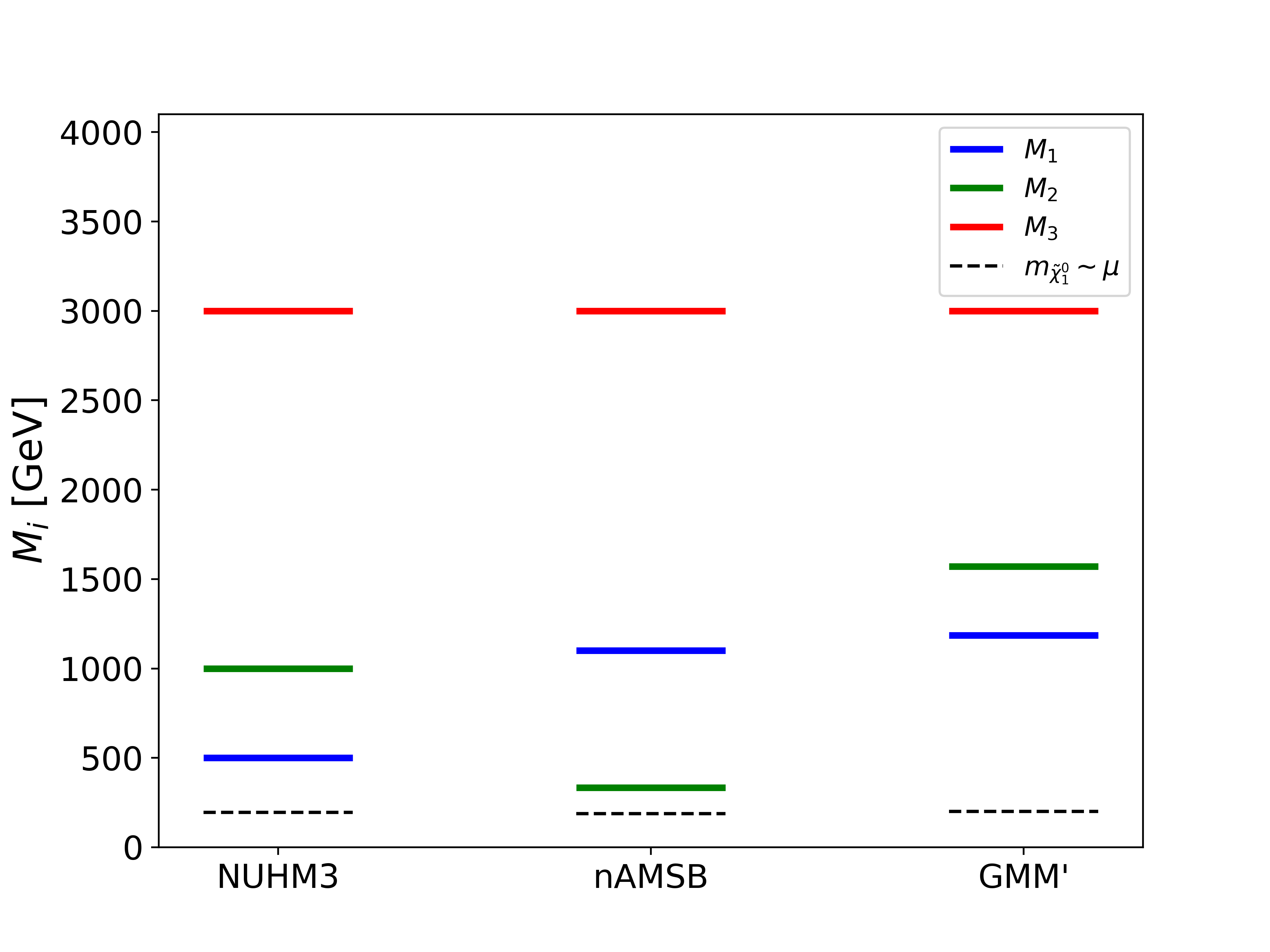
Figure 1: Figurative plot of gaugino/higgsino masses in the three paradigm natural SUSY models with $m_{\tilde{g}}\simeq 3$ TeV and $\mu=200$ GeV.

3 Revealing the gaugino code, naturally, at high-lumi LHC

The LHC has two promising avenues towards decoding the natural gaugino code, namely by observing 1. higgsino pair production and 2. wino pair production. It turns out each of these channels is quite distinctive to the case of natural SUSY models and signals should gradually emerge as LHC accrues higher and higher integrated luminosity. From Run 2 data, both ATLAS and CMS seem to have small $2\sigma$ excesses in the higgsino pair production channel[54, 55]. It is thus of great interest to see if these excesses build up or fade away with the Run 3 and HL-LHC data sets.

3.1 Higgsino pair production

Charged higgsino pair production $pp\rightarrow\tilde{\chi}_{1}^{+}\tilde{\chi}_{1}^{-}$ followed by $\tilde{\chi}_{1}^{\pm}\rightarrow\tilde{\chi}_{1}^{0}f\bar{f}^{\prime}$ decay (where $f$ stands for SM fermions) typically yields very soft visible decay products and $\not\!\!\!{E_{T}}$ and a rather indistinct signature. Neutral higgsino pair production[56]

$$pp\rightarrow\tilde{\chi}_{2}^{0}\tilde{\chi}_{1}^{0}\ \ {\rm with}\ \ \ \tilde{\chi}_{2}^{0}\rightarrow\tilde{\chi}_{1}^{0}f\bar{f}$$ (25)

may also lead to very low visible energy, unless the scattering reaction recoils from a hard initial state quark/gluon radiation[57, 58, 59] (ISR). In this latter case, letting $f$ be $e$ or $\mu$, then we expect soft opposite-sign dilepton plus jet plus $\not\!\!\!{E_{T}}$ production (OSDLJMET) where the opposite-sign (OS) dilepton pair has invariant mass $m(\ell\bar{\ell})$ kinematically bounded by $m_{\tilde{\chi}_{2}^{0}}-m_{\tilde{\chi}_{1}^{0}}$. Thus, in the signal $m(\ell\bar{\ell})$ distribution, we expect an excess beyond SM expectations for $m(\ell\bar{\ell})<m_{\tilde{\chi}_{2}^{0}}-m_{\tilde{\chi}_{1}^{0}}$ while data should agree with SM expectations for higher invariant dilepton masses.[60] Along with offering a distinctive signal channel for natural SUSY models at HL-LHC, this channel also provides a direct measure of the neutral higgsino mass difference $m_{\tilde{\chi}_{2}^{0}}-m_{\tilde{\chi}_{1}^{0}}$. A rough estimate of the superpotential $\mu$ parameter may also be gleaned from this channel based on total rate since $m_{\tilde{\chi}_{2}^{0}}\sim m_{\tilde{\chi}_{1}^{0}}\sim\mu$ and the total production rate mainly depends on the raw higgsino masses. In fact, the exclusion limits are typically plotted in the $m_{\tilde{\chi}_{2}^{0}}$ vs $m_{\tilde{\chi}_{2}^{0}}-m_{\tilde{\chi}_{1}^{0}}$ plane[61]. More refined cuts for extracting the OSDLJMET signal have recently been presented in Ref’s. [62, 63].

3.2 Wino pair production

Another distinctive SUSY discovery channel which is endemic to natural SUSY models is the clean same-sign diboson signal (SSdB) which arises from wino pair production:

$$pp\rightarrow\tilde{\chi}_{2}^{+}\tilde{\chi}_{3,4}^{0}\ \ {\rm with}\ \ \tilde{\chi}_{2}^{+}\rightarrow W^{+}\tilde{\chi}_{1,2}\ \ {\rm and}\ \ \tilde{\chi}_{3,4}\rightarrow W^{\pm}\tilde{\chi}_{1}^{\mp}$$ (26)

where the $\tilde{\chi}_{2}^{\pm}$ is the charged wino and $\tilde{\chi}_{3}^{0}$ is the neutral wino in nAMSB or $\tilde{\chi}_{4}^{0}$ is the neutral wino in GMM’ or NUHM3. Since the visible decay products of the daughter higgsinos are very soft, and upon leptonic decays of the final state $W$ bosons, this reaction leads half the time to a hadronically clean (aside from usual ISR) same-sign dilepton $+\not\!\!\!{E_{T}}$ final state which has very low SM backgrounds[64, 65, 66]. This is different from the older same-sign dilepton signals arising from gluino and squark pair production which would be accompanied by multiple hard jets[67, 68, 69, 70].

Due to the required two $W$-boson leptonic branching fractions, the rate for this channel for the current LHC Run 2 data set is typically expected around the 1-event level, so at present no search limits are available from this channel. However, as more integrated luminosity accrues, this channel will become more and more important due to the extremely low SM background levels. Since the production rate mainly depends on $m(wino)$, and the wino branching fractions to $W$ bosons is well-known and theoretically stable, the direct production rate can yield a measure of the gaugino mass $M_{2}$[66]. In Ref. [66], it is estimated that with 3 ab^-1 of integrated luminosity (corresponding to $\sim 10-100$ events), HL-LHC should be able to determine $m(wino)$ to around the 5-10% level based on signal rate alone, including statistical errors.

3.3 Decoding the gaugino code at HL-LHC

Next, we perform string landscape scans of soft SUSY breaking parameters assuming the textbook case of an $n=1$ power-law landscape draw to large soft terms. Each class of soft terms (gaugino mass, scalar mass, $A$-terms) should scan independently on the landscape owing to the different functional dependence of soft terms on hidden sector fields for different string compactification possibilities[21]. Thus, we scan NUHM3 over the range

• $m_{0}(1,2):0.1-60$ TeV,

• $m_{0}(3):0.1-20$ TeV,

• $m_{1/2}:0.5-10$ TeV,

• $A_{0}:-50-0$ TeV (negative only),

at first for fixed $\mu=200$ GeV (since $\mu$ is not a soft term but arises from whatever solution to the SUSY $\mu$ problem is assumed). For each parameter set, the expected value of the weak scale in each pocket universe is computed from $m_{weak}^{PU}=m_{Z}\sqrt{\Delta_{EW}/2}$ and solutions with $m_{weak}^{PU}>4m_{weak}^{OU}$ are rejected as lying beyond the ABDS window. (An important technical point is that the scan range upper limits must be selected to be beyond the upper limits imposed by the anthropic ABDS window.) To gain probability distributions for Higgs and sparticle masses in our universe, then as a final step $m_{Z}^{PU}$ must be adjusted (but not finetuned!) to our value $m_{Z}^{OU}=91.2$ GeV.

For the nAMSB model, our landscape scan is over[18]

• $m_{3/2}:\ 80-400$ TeV,

• $m_{0}(1,2):\ 1-20$ TeV,

• $m_{0}(3):\ 1-10$ TeV,

• $A_{0}:\ 0-20$ TeV (positive only).

For GMM’, our scan follows Ref. [19] with fixed $m_{3/2}=20$ TeV:

• $\alpha:\ 3-25$ (with $\alpha^{1}$ draw),

• $c_{m1,2}=(16\pi^{2}/\alpha)^{2}$

• $\sqrt{c_{m3}\alpha^{2}}:\ 3-80$ and

• $(a_{3}\alpha):\ 3-100$

For all cases, we scan with a linear draw $m_{A}:0.25-10$ TeV and uniformly over $\tan\beta:\ 3-60$.

The results of our scans are plotted in Fig. 2 in the $\Delta m^{0}\equiv m_{\tilde{\chi}_{2}^{0}}-m_{\tilde{\chi}_{1}^{0}}$ vs. $M_{2}$ plane. Green dots denote nAMSB points, blue dots denote NUHM3 points and red dots denote GMM’ points. From Fig. 2, we see the three models inhabit somewhat different locusses in the plane. The green nAMSB points extend to rather large $\Delta m_{0}$ values –as high as $\Delta m^{0}\sim 60$ GeV– since in this case the light winos can mix with the higgsinos, thus breaking the expected inter-higgsino mass degeneracy. Also, the range in $M_{2}$ for nAMSB points only extends as high as $\sim 750$ GeV. In contrast, the NUHM3 model with unified gaugino masses has a maximal $\Delta m^{0}\sim 30$ GeV but $M_{2}$ can extend as high as $\sim 1250$ GeV where $\Delta m^{0}\sim 7$ GeV. The GMM’ is intermediate between these models, since it has mixed gravity/AMSB mediation. At low $M_{2}$, where $\alpha$ is small, it looks more like AMSB spectra and has a slight overlap with the green points, while at high $\alpha$ values it looks more like gravity-mediation and lies closer to the blue points, although the compressed GMM’ gaugino spectrum allows $M_{2}$ to extend much further, as high as $M_{2}\sim 2$ TeV where $\Delta m^{0}$ is as low as $\sim 4$ GeV. Notice in all cases $\Delta m^{0}$ never reaches below the few GeV case, since for that to occur, $M_{2}$ values would have to be so high that $\Sigma_{u}^{u}(m(wino))$ would become unnatural[73], and lie outside the ABDS window.

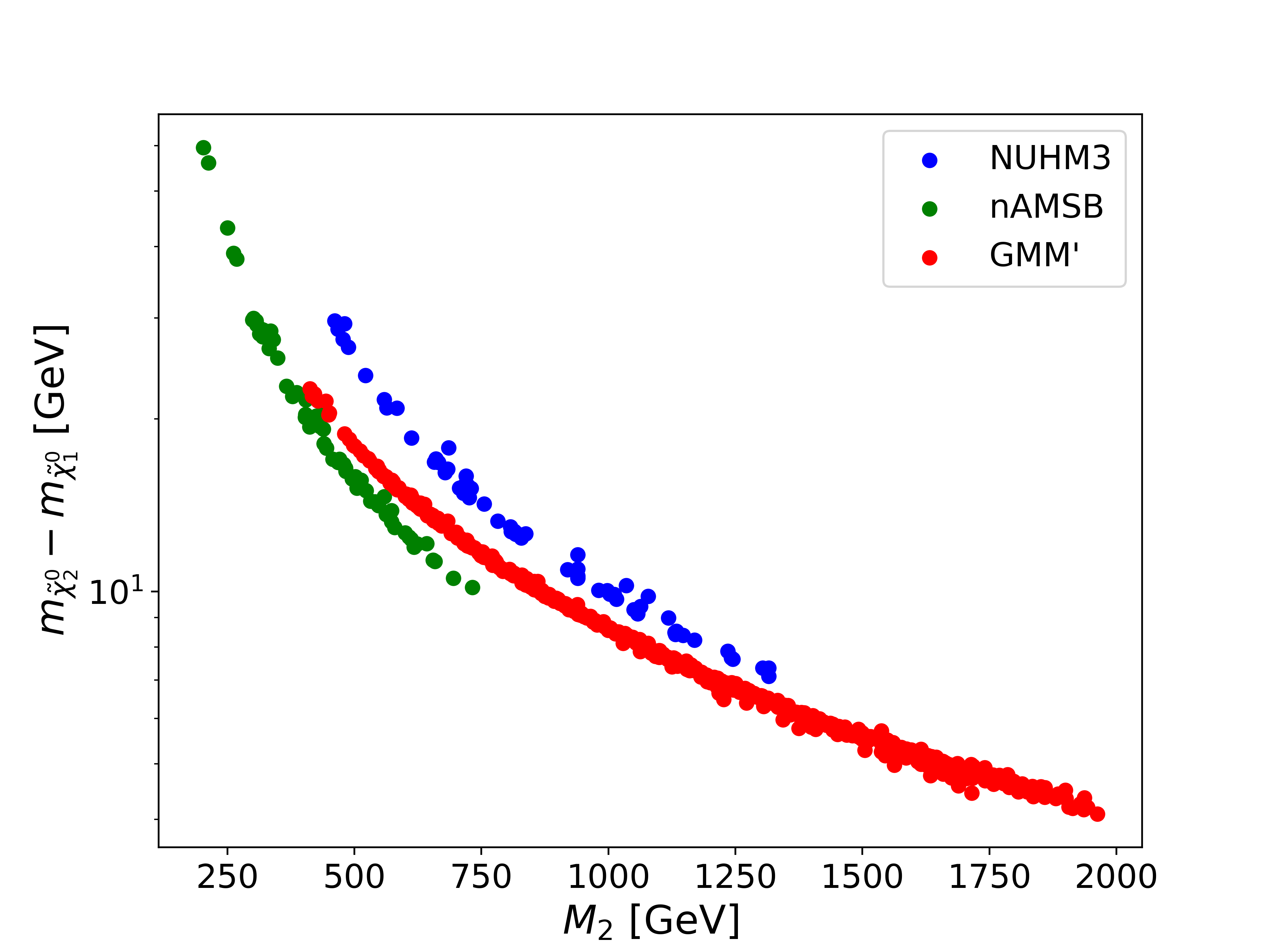
Figure 2: Locus of landscape scan points from the NUHM3 model, the nAMSB model and GMM’ model in the $m_{\tilde{\chi}_{2}^{0}}-m_{\tilde{\chi}_{1}^{0}}$ vs. $m_{\tilde{\chi}_{2}^{+}}\simeq M_{2}$ plane for fixed value $\mu=200$ GeV.

In Fig. 3, we again plot the locus of $n=1$ landscape scan points in the $m_{\tilde{\chi}_{2}^{0}}-m_{\tilde{\chi}_{1}^{0}}$ vs. $M_{2}$ plane, but this time including a uniform scan over $\mu:100-350$ GeV, in case the $\mu$ parameter cannot be well-measured. In this case, the model scan points broaden out and have some substantial overlap in the intermediate mass region. Nonetheless, the landscape scan regions still maintain some degree of separation as shown by the colored dots, so depending on where the ultimate measure values of $\Delta m^{0}$ and $m_{\tilde{\chi}_{1}^{\pm}}$ lay, the locus may or may not lie within a distinguishable region. Clearly, a more precide measured value of $\mu$ will help aid in this enterprise.

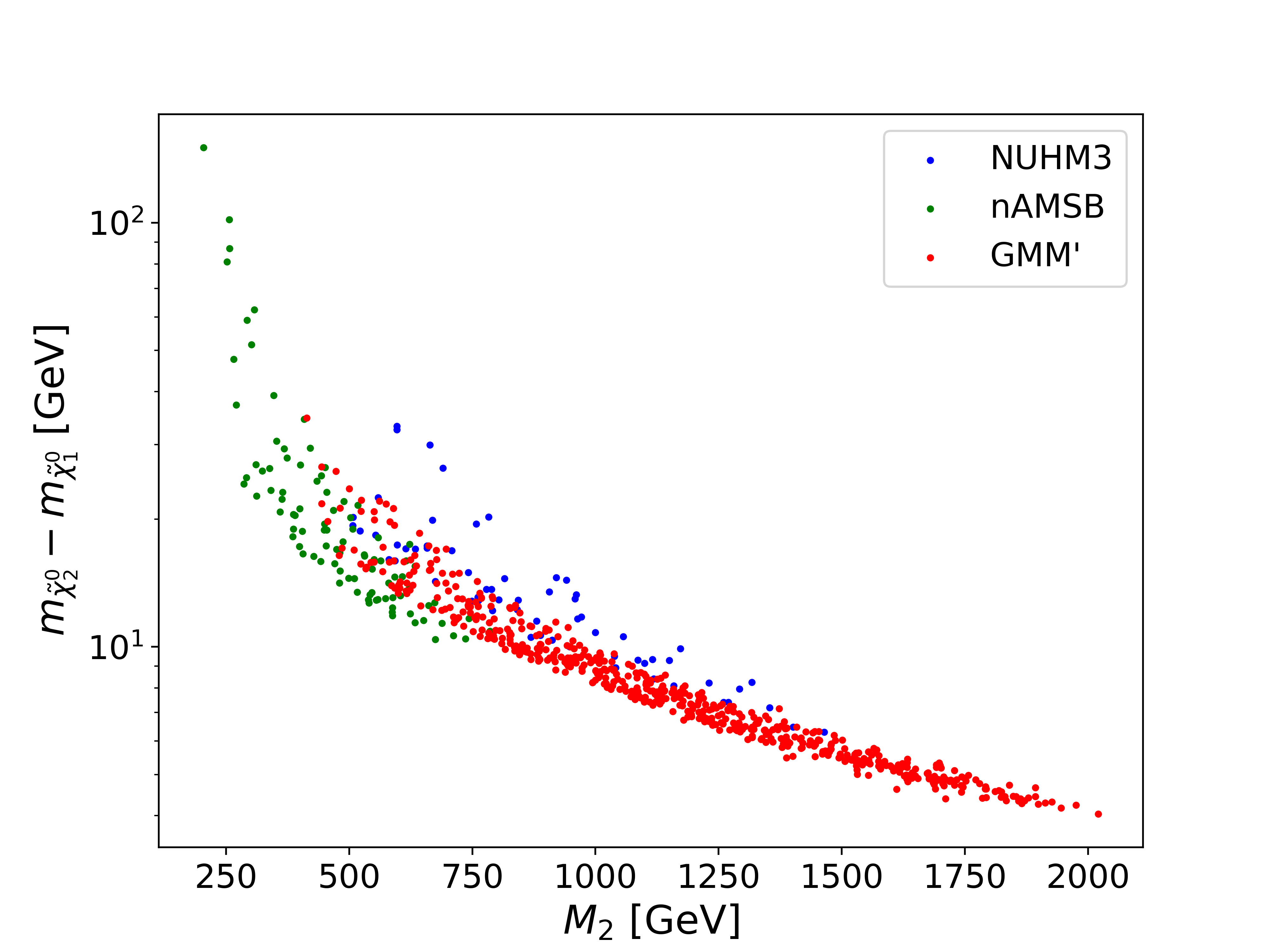
Figure 3: Locus of landscape scan points from the NUHM3 model, the nAMSB model and GMM’ model in the $m_{\tilde{\chi}_{2}^{0}}-m_{\tilde{\chi}_{1}^{0}}$ vs. $m_{\tilde{\chi}_{2}^{+}}\simeq M_{2}$ plane for a uniform scan over $\mu=100-350$ GeV.

4 Conclusions

String flux compactifications on a Calabi-Yau manifold with special holonomy preserve some remnant $N=1$ supersymmetry which provides a ’t Hooft technical natural solution to the big hierarchy problem. The question then is: what is the scale of SUSY breaking and does the subsequent SUSY spectrum avoid the little hierarchy problem based on practical naturalness? Rather general arguments from the string landscape favor a power-law draw to large soft terms tempered by the anthropic requirement that the derived value of the weak scale lie within the so-called ABDS window. In this case, EW natural SUSY models are most likely to emerge as opposed to finetuned SUSY models since the latter viable parameter space shrinks to a relatvely tiny volume compared to natural models (one must happen upon the finetuned parameters that lead to a weak scale not-too-far removed from its measured value in our universe. These natural models would be characterized by first/second generation scalars in the 10-40 TeV range while top-squarks inhabit the few TeV range and higgsinos lie not to far from $m_{weak}$ in the 100-350 GeV range. Within the context of natural models, three main paradigms are viable, distinguished by the orientation of the gaugino masses: unified gaugino masses as in the NUHM3 model, AMSB gaugino masses as in nAMSB and mirage mediated gaugino masses as in the GMM’ model.

Can forthcoming data from HL-LHC distinguish these cases, thus decoding the gaugino code? Two avenues to detection of natural SUSY models lie in the ODLJMET signal from higgsino pair production and the SSdB signature arising from wino pair production. The first admits a precise measurement of $\Delta m^{0}=m_{\tilde{\chi}_{2}^{0}}-m_{\tilde{\chi}_{1}^{0}}$ via the expected edge in the $m(\ell\bar{\ell})$ distribution while wino pair production may allow extraction of the wino mass $M_{2}$ from the total rate of SSdB production. By placing these measurements within the $\Delta m^{0}$ vs. $M_{2}$ plane, one may well be able to decode the gaugino code since SUSY models predict the different cases may inhabit distinctive regions of this parameter plane

Acknowledgements:

VB gratefully acknowledges support from the William F. Vilas estate. HB gratefully acknowledges support from the Avenir Foundation.

References

- [1] P. Candelas, G. T. Horowitz, A. Strominger, E. Witten, Vacuum configurations for superstrings, Nucl. Phys. B 258 (1985) 46–74. doi:10.1016/0550-3213(85)90602-9.
- [2] E. Witten, Dynamical Breaking of Supersymmetry, Nucl. Phys. B 188 (1981) 513. doi:10.1016/0550-3213(81)90006-7.
- [3] R. K. Kaul, Gauge Hierarchy in a Supersymmetric Model, Phys. Lett. B 109 (1982) 19–24. doi:10.1016/0370-2693(82)90453-1.
- [4] A. Canepa, Searches for Supersymmetry at the Large Hadron Collider, Rev. Phys. 4 (2019) 100033. doi:10.1016/j.revip.2019.100033.
- [5] G. Aad, et al., The quest to discover supersymmetry at the ATLAS experimentarXiv:2403.02455.
- [6] R. Bousso, J. Polchinski, Quantization of four form fluxes and dynamical neutralization of the cosmological constant, JHEP 06 (2000) 006. arXiv:hep-th/0004134, doi:10.1088/1126-6708/2000/06/006.
- [7] L. Susskind, The Anthropic landscape of string theory (2003) 247–266arXiv:hep-th/0302219.
- [8] S. Ashok, M. R. Douglas, Counting flux vacua, JHEP 01 (2004) 060. arXiv:hep-th/0307049, doi:10.1088/1126-6708/2004/01/060.
- [9] M. R. Douglas, S. Kachru, Flux compactification, Rev. Mod. Phys. 79 (2007) 733–796. arXiv:hep-th/0610102, doi:10.1103/RevModPhys.79.733.
- [10] S. Weinberg, Anthropic Bound on the Cosmological Constant, Phys. Rev. Lett. 59 (1987) 2607. doi:10.1103/PhysRevLett.59.2607.
- [11] N. Arkani-Hamed, S. Dimopoulos, S. Kachru, Predictive landscapes and new physics at a TeVarXiv:hep-th/0501082.
- [12] H. Baer, X. Tata, Weak scale supersymmetry: From superfields to scattering events, Cambridge University Press, 2006.
- [13] M. R. Douglas, Statistical analysis of the supersymmetry breaking scalearXiv:hep-th/0405279.
- [14] L. Susskind, Supersymmetry breaking in the anthropic landscape, in: From Fields to Strings: Circumnavigating Theoretical Physics: A Conference in Tribute to Ian Kogan, 2004, pp. 1745–1749. arXiv:hep-th/0405189, doi:10.1142/9789812775344_0040.
- [15] H. Baer, V. Barger, M. Savoy, H. Serce, The Higgs mass and natural supersymmetric spectrum from the landscape, Phys. Lett. B 758 (2016) 113–117. arXiv:1602.07697, doi:10.1016/j.physletb.2016.05.010.
- [16] V. Agrawal, S. M. Barr, J. F. Donoghue, D. Seckel, Viable range of the mass scale of the standard model, Phys. Rev. D 57 (1998) 5480–5492. arXiv:hep-ph/9707380, doi:10.1103/PhysRevD.57.5480.
- [17] H. Baer, V. Barger, H. Serce, K. Sinha, Higgs and superparticle mass predictions from the landscape, JHEP 03 (2018) 002. arXiv:1712.01399, doi:10.1007/JHEP03(2018)002.
- [18] H. Baer, V. Barger, J. Bolich, J. Dutta, D. Sengupta, Natural anomaly mediation from the landscape with implications for LHC SUSY searches, Phys. Rev. D 109 (3) (2024) 035011. arXiv:2311.18120, doi:10.1103/PhysRevD.109.035011.
- [19] H. Baer, V. Barger, D. Sengupta, Mirage mediation from the landscape, Phys. Rev. Res. 2 (1) (2020) 013346. arXiv:1912.01672, doi:10.1103/PhysRevResearch.2.013346.
- [20] H. Baer, V. Barger, S. Salam, D. Sengupta, K. Sinha, Status of weak scale supersymmetry after LHC Run 2 and ton-scale noble liquid WIMP searches, Eur. Phys. J. ST 229 (21) (2020) 3085–3141. arXiv:2002.03013, doi:10.1140/epjst/e2020-000020-x.
- [21] H. Baer, V. Barger, S. Salam, D. Sengupta, String landscape guide to soft SUSY breaking terms, Phys. Rev. D 102 (7) (2020) 075012. arXiv:2005.13577, doi:10.1103/PhysRevD.102.075012.
- [22] K. Choi, H. P. Nilles, The Gaugino code, JHEP 04 (2007) 006. arXiv:hep-ph/0702146, doi:10.1088/1126-6708/2007/04/006.
- [23] S. K. Soni, H. A. Weldon, Analysis of the Supersymmetry Breaking Induced by N=1 Supergravity Theories, Phys. Lett. B 126 (1983) 215–219. doi:10.1016/0370-2693(83)90593-2.
- [24] V. S. Kaplunovsky, J. Louis, Model independent analysis of soft terms in effective supergravity and in string theory, Phys. Lett. B 306 (1993) 269–275. arXiv:hep-th/9303040, doi:10.1016/0370-2693(93)90078-V.
- [25] A. Brignole, L. E. Ibanez, C. Munoz, Towards a theory of soft terms for the supersymmetric Standard Model, Nucl. Phys. B 422 (1994) 125–171, [Erratum: Nucl.Phys.B 436, 747–748 (1995)]. arXiv:hep-ph/9308271, doi:10.1016/0550-3213(94)00068-9.
- [26] R. L. Arnowitt, P. Nath, Supersymmetry and Supergravity: Phenomenology and Grand Unification, in: 6th Summer School Jorge Andre Swieca on Nuclear Physics, 1993. arXiv:hep-ph/9309277.
- [27] G. L. Kane, C. F. Kolda, L. Roszkowski, J. D. Wells, Study of constrained minimal supersymmetry, Phys. Rev. D 49 (1994) 6173–6210. arXiv:hep-ph/9312272, doi:10.1103/PhysRevD.49.6173.
- [28] H. Baer, V. Barger, P. Huang, A. Mustafayev, X. Tata, Radiative natural SUSY with a 125 GeV Higgs boson, Phys. Rev. Lett. 109 (2012) 161802. arXiv:1207.3343, doi:10.1103/PhysRevLett.109.161802.
- [29] H. Baer, V. Barger, P. Huang, D. Mickelson, A. Mustafayev, X. Tata, Radiative natural supersymmetry: Reconciling electroweak fine-tuning and the Higgs boson mass, Phys. Rev. D 87 (11) (2013) 115028. arXiv:1212.2655, doi:10.1103/PhysRevD.87.115028.
- [30] N. Arkani-Hamed, H. Murayama, Can the supersymmetric flavor problem decouple?, Phys. Rev. D 56 (1997) R6733–R6737. arXiv:hep-ph/9703259, doi:10.1103/PhysRevD.56.R6733.
- [31] H. Baer, V. Barger, D. Sengupta, Landscape solution to the SUSY flavor and CP problems, Phys. Rev. Res. 1 (3) (2019) 033179. arXiv:1910.00090, doi:10.1103/PhysRevResearch.1.033179.
- [32] E. Cremmer, S. Ferrara, L. Girardello, A. Van Proeyen, Yang-Mills Theories with Local Supersymmetry: Lagrangian, Transformation Laws and SuperHiggs Effect, Nucl. Phys. B 212 (1983) 413. doi:10.1016/0550-3213(83)90679-X.
- [33] W. Buchmuller, K. Hamaguchi, O. Lebedev, M. Ratz, Local grand unification, in: GUSTAVOFEST: Symposium in Honor of Gustavo C. Branco: CP Violation and the Flavor Puzzle, 2005, pp. 143–156. arXiv:hep-ph/0512326.
- [34] H. P. Nilles, P. K. S. Vaudrevange, Geography of Fields in Extra Dimensions: String Theory Lessons for Particle Physics, Mod. Phys. Lett. A 30 (10) (2015) 1530008. arXiv:1403.1597, doi:10.1142/S0217732315300086.
- [35] L. Randall, R. Sundrum, Out of this world supersymmetry breaking, Nucl. Phys. B 557 (1999) 79–118. arXiv:hep-th/9810155, doi:10.1016/S0550-3213(99)00359-4.
- [36] G. F. Giudice, M. A. Luty, H. Murayama, R. Rattazzi, Gaugino mass without singlets, JHEP 12 (1998) 027. arXiv:hep-ph/9810442, doi:10.1088/1126-6708/1998/12/027.
- [37] J. A. Bagger, T. Moroi, E. Poppitz, Anomaly mediation in supergravity theories, JHEP 04 (2000) 009. arXiv:hep-th/9911029, doi:10.1088/1126-6708/2000/04/009.
- [38] J. D. Wells, PeV-scale supersymmetry, Phys. Rev. D 71 (2005) 015013. arXiv:hep-ph/0411041, doi:10.1103/PhysRevD.71.015013.
- [39] N. Arkani-Hamed, S. Dimopoulos, G. F. Giudice, A. Romanino, Aspects of split supersymmetry, Nucl. Phys. B 709 (2005) 3–46. arXiv:hep-ph/0409232, doi:10.1016/j.nuclphysb.2004.12.026.
- [40] A. Arvanitaki, N. Craig, S. Dimopoulos, G. Villadoro, Mini-Split, JHEP 02 (2013) 126. arXiv:1210.0555, doi:10.1007/JHEP02(2013)126.
- [41] T. Gherghetta, G. F. Giudice, J. D. Wells, Phenomenological consequences of supersymmetry with anomaly induced masses, Nucl. Phys. B 559 (1999) 27–47. arXiv:hep-ph/9904378, doi:10.1016/S0550-3213(99)00429-0.
- [42] J. L. Feng, T. Moroi, Supernatural supersymmetry: Phenomenological implications of anomaly mediated supersymmetry breaking, Phys. Rev. D 61 (2000) 095004. arXiv:hep-ph/9907319, doi:10.1103/PhysRevD.61.095004.
- [43] T. Cohen, M. Lisanti, A. Pierce, T. R. Slatyer, Wino Dark Matter Under Siege, JCAP 10 (2013) 061. arXiv:1307.4082, doi:10.1088/1475-7516/2013/10/061.
- [44] J. Fan, M. Reece, In Wino Veritas? Indirect Searches Shed Light on Neutralino Dark Matter, JHEP 10 (2013) 124. arXiv:1307.4400, doi:10.1007/JHEP10(2013)124.
- [45] H. Baer, V. Barger, H. Serce, SUSY under siege from direct and indirect WIMP detection experiments, Phys. Rev. D 94 (11) (2016) 115019. arXiv:1609.06735, doi:10.1103/PhysRevD.94.115019.
- [46] H. Baer, V. Barger, D. Mickelson, M. Padeffke-Kirkland, SUSY models under siege: LHC constraints and electroweak fine-tuning, Phys. Rev. D 89 (11) (2014) 115019. arXiv:1404.2277, doi:10.1103/PhysRevD.89.115019.
- [47] H. Baer, V. Barger, D. Sengupta, Anomaly mediated SUSY breaking model retrofitted for naturalness, Phys. Rev. D 98 (1) (2018) 015039. arXiv:1801.09730, doi:10.1103/PhysRevD.98.015039.
- [48] K. Choi, A. Falkowski, H. P. Nilles, M. Olechowski, Soft supersymmetry breaking in KKLT flux compactification, Nucl. Phys. B 718 (2005) 113–133. arXiv:hep-th/0503216, doi:10.1016/j.nuclphysb.2005.04.032.
- [49] S. Kachru, R. Kallosh, A. D. Linde, S. P. Trivedi, De Sitter vacua in string theory, Phys. Rev. D 68 (2003) 046005. arXiv:hep-th/0301240, doi:10.1103/PhysRevD.68.046005.
- [50] H. P. Nilles, Gaugino Condensation and Supersymmetry Breakdown, Int. J. Mod. Phys. A 5 (1990) 4199–4224. doi:10.1142/S0217751X90001744.
- [51] I. R. Klebanov, M. J. Strassler, Supergravity and a confining gauge theory: Duality cascades and chi SB resolution of naked singularities, JHEP 08 (2000) 052. arXiv:hep-th/0007191, doi:10.1088/1126-6708/2000/08/052.
- [52] A. Falkowski, O. Lebedev, Y. Mambrini, SUSY phenomenology of KKLT flux compactifications, JHEP 11 (2005) 034. arXiv:hep-ph/0507110, doi:10.1088/1126-6708/2005/11/034.
- [53] H. Baer, V. Barger, H. Serce, X. Tata, Natural generalized mirage mediation, Phys. Rev. D 94 (11) (2016) 115017. arXiv:1610.06205, doi:10.1103/PhysRevD.94.115017.
- [54] G. Aad, et al., Searches for electroweak production of supersymmetric particles with compressed mass spectra in 13 TeV collisions with the ATLAS detector, Phys. Rev. D 101 (5) (2020) 052005. arXiv:1911.12606, doi:10.1103/PhysRevD.101.052005.
- [55] A. Tumasyan, et al., Search for supersymmetry in final states with two or three soft leptons and missing transverse momentum in proton-proton collisions at = 13 TeV, JHEP 04 (2022) 091. arXiv:2111.06296, doi:10.1007/JHEP04(2022)091.
- [56] H. Baer, V. Barger, P. Huang, Hidden SUSY at the LHC: the light higgsino-world scenario and the role of a lepton collider, JHEP 11 (2011) 031. arXiv:1107.5581, doi:10.1007/JHEP11(2011)031.
- [57] Z. Han, G. D. Kribs, A. Martin, A. Menon, Hunting quasidegenerate Higgsinos, Phys. Rev. D 89 (7) (2014) 075007. arXiv:1401.1235, doi:10.1103/PhysRevD.89.075007.
- [58] H. Baer, A. Mustafayev, X. Tata, Monojet plus soft dilepton signal from light higgsino pair production at LHC14, Phys. Rev. D 90 (11) (2014) 115007. arXiv:1409.7058, doi:10.1103/PhysRevD.90.115007.
- [59] C. Han, D. Kim, S. Munir, M. Park, Accessing the core of naturalness, nearly degenerate higgsinos, at the LHC, JHEP 04 (2015) 132. arXiv:1502.03734, doi:10.1007/JHEP04(2015)132.
- [60] R. Kitano, Y. Nomura, Supersymmetry, naturalness, and signatures at the LHC, Phys. Rev. D 73 (2006) 095004. arXiv:hep-ph/0602096, doi:10.1103/PhysRevD.73.095004.
- [61] H. Baer, V. Barger, S. Salam, D. Sengupta, X. Tata, The LHC higgsino discovery plane for present and future SUSY searches, Phys. Lett. B 810 (2020) 135777. arXiv:2007.09252, doi:10.1016/j.physletb.2020.135777.
- [62] H. Baer, V. Barger, D. Sengupta, X. Tata, New angular and other cuts to improve the Higgsino signal at the LHC, Phys. Rev. D 105 (9) (2022) 095017. arXiv:2109.14030, doi:10.1103/PhysRevD.105.095017.
- [63] H. Baer, V. Barger, D. Sengupta, X. Tata, Angular cuts to reduce the background to the higgsino signal at the LHC, in: Snowmass 2021, 2022. arXiv:2203.03700.
- [64] H. Baer, V. Barger, P. Huang, D. Mickelson, A. Mustafayev, W. Sreethawong, X. Tata, Same sign diboson signature from supersymmetry models with light higgsinos at the LHC, Phys. Rev. Lett. 110 (15) (2013) 151801. arXiv:1302.5816, doi:10.1103/PhysRevLett.110.151801.
- [65] H. Baer, V. Barger, P. Huang, D. Mickelson, A. Mustafayev, W. Sreethawong, X. Tata, Radiatively-driven natural supersymmetry at the LHC, JHEP 12 (2013) 013, [Erratum: JHEP 06, 053 (2015)]. arXiv:1310.4858, doi:10.1007/JHEP12(2013)013.
- [66] H. Baer, V. Barger, J. S. Gainer, M. Savoy, D. Sengupta, X. Tata, Aspects of the same-sign diboson signature from wino pair production with light higgsinos at the high luminosity LHC, Phys. Rev. D 97 (3) (2018) 035012. arXiv:1710.09103, doi:10.1103/PhysRevD.97.035012.
- [67] H. Baer, X. Tata, J. Woodside, SEARCHING FOR 100-GeV - 300-GeV GLUINOS AT THE TEVATRON AND SSC, in: 1988 DPF Summer Study on High-energy Physics in the 1990s (Snowmass 88), 1988.
- [68] R. M. Barnett, J. F. Gunion, H. E. Haber, LIKE SIGN DILEPTONS AS A SIGNAL FOR GLUINO PRODUCTION, in: 1988 DPF Summer Study on High-energy Physics in the 1990s (Snowmass 88), 1988.
- [69] H. Baer, X. Tata, J. Woodside, Gluino Cascade Decay Signatures at the Tevatron Collider, Phys. Rev. D 41 (1990) 906–915. doi:10.1103/PhysRevD.41.906.
- [70] R. M. Barnett, J. F. Gunion, H. E. Haber, Discovering supersymmetry with like sign dileptons, Phys. Lett. B 315 (1993) 349–354. arXiv:hep-ph/9306204, doi:10.1016/0370-2693(93)91623-U.
- [71] F. E. Paige, S. D. Protopopescu, H. Baer, X. Tata, ISAJET 7.69: A Monte Carlo event generator for pp, anti-p p, and e+e- reactionsarXiv:hep-ph/0312045.
- [72] K. J. Bae, H. Baer, V. Barger, D. Sengupta, Revisiting the SUSY problem and its solutions in the LHC era, Phys. Rev. D 99 (11) (2019) 115027. arXiv:1902.10748, doi:10.1103/PhysRevD.99.115027.
- [73] H. Baer, V. Barger, M. Savoy, Upper bounds on sparticle masses from naturalness or how to disprove weak scale supersymmetry, Phys. Rev. D 93 (3) (2016) 035016. arXiv:1509.02929, doi:10.1103/PhysRevD.93.035016.