DNA-SE: Towards Deep Neural-Nets Assisted Semiparametric Estimation

Abstract

Semiparametric statistics play a pivotal role in a wide range of domains, including but not limited to missing data, causal inference, and transfer learning, to name a few. In many settings, semiparametric theory leads to (nearly) statistically optimal procedures that yet involve numerically solving Fredholm integral equations of the second kind. Traditional numerical methods, such as polynomial or spline approximations, are difficult to scale to multi-dimensional problems. Alternatively, statisticians may choose to approximate the original integral equations by ones with closed-form solutions, resulting in computationally more efficient, but statistically suboptimal or even incorrect procedures. To bridge this gap, we propose a novel framework by formulating the semiparametric estimation problem as a bi-level optimization problem; and then we develop a scalable algorithm called Deep Neural-Nets Assisted Semiparametric Estimation (${\mathsf{DNA\mbox{-}SE}}$) by leveraging the universal approximation property of Deep Neural-Nets (DNN) to streamline semiparametric procedures. Through extensive numerical experiments and a real data analysis, we demonstrate the numerical and statistical advantages of ${\mathsf{DNA\mbox{-}SE}}$ over traditional methods. To the best of our knowledge, we are the first to bring DNN into semiparametric statistics as a numerical solver of integral equations in our proposed general framework.

1 Introduction

Deep Neural-Nets (DNN) have made unprecedented progress in a variety of scientific and industrial problems, such as image classification (Krizhevsky et al., 2012), natural language processing (Vaswani et al., 2017), and scientific computing (E & Yu, 2018). Recently, the statistical literature has also garnered increasing interests in deploying DNN to solve statistical problems that baffled traditional methods, for example, nonparametric regression (Chen & White, 1999; Suzuki, 2019; Schmidt-Hieber, 2020; Padilla et al., 2022) and nonparametric density estimation (Liu et al., 2021b; Liang, 2021). A common theme in these applications is to view DNN as an alternative method to approximate infinite-dimensional nonparametric models, conventionally done by splines, polynomials, etc. (Giné & Nickl, 2016).

Interpretability is at the core of many statistical problems. A conceptually appealing statistical paradigm is semiparametric statistics (including semiparametric statistical models, methods and related theory). In semiparametric statistics, one models the part of the Data Generating Process (DGP) of scientific interest with low-dimensional parametric models to improve interpretability, while leaving the remaining part (termed as nuisance parameters) either completely unspecified or modeled by infinite-dimensional nonparametric models to avoid unnecessary model misspecification bias (Newey, 1990; Bickel et al., 1998). As a result, semiparametric statistics have been very popular in problems calling for both interpretability and robustness against model misspecification, such as missing data (Robins et al., 1994), causal inference (van der Laan & Robins, 2003), and more recently, transfer learning (Qiu et al., 2023; Tian et al., 2023). It is natural to employ DNN to estimate the infinite-dimensional nuisance parameters in semiparametric models, an extension of the aforementioned idea from nonparametric statistics. In fact, this is the route that most recent semiparametric statistics literature has taken (Farrell et al., 2021; Shi et al., 2021; Zhong et al., 2022; Xu et al., 2022; Kompa et al., 2022; Chernozhukov et al., 2022; Chen et al., 2023a, 2024).

In this paper, we take a different path and instead propose to treat DNN as a numerical solver for semiparametric statistics. Here is our motivation. All the above cited works on semiparametric statistics are special cases, where the statistically optimal (i.e. semiparametric efficient) estimator for the parameter of scientific interest has closed-form. In general, however, semiparametric theory can lead to nearly statistically optimal estimators that depend on the solution of Fredholm integral equations of the second kind (Bickel et al., 1998). These integral equations often: (1) do not have closed-form solutions; and (2) depend on the unknown parameter of interest, calling for complicated iterative methods (Robins et al., 1994). As shown in our numerical experiments in Section 4, using traditional methods such as polynomials/splines (Bellour et al., 2016) or approximately inverting the integral kernel (Atkinson, 1967) to approximate the solution does not always lead to optimal or satisfactory estimators in practice. In certain cases, statisticians may derive alternative estimators with closed-forms, but this strategy generally leads to statistically suboptimal or sometimes even inconsistent estimators (Zhao & Ma, 2022; Liu et al., 2021a; Yang, 2022).

To bridge this gap, inspired by recent works using DNN as a new-generation numerical method for scientific computing (E & Yu, 2018; Raissi et al., 2019; Li et al., 2020), we propose a novel framework by formulating the semiparametric estimation problem as a bi-level optimization problem; and then we develop a scalable algorithm called Deep Neural-Nets Assisted Semiparametric Estimation (${\mathsf{DNA\mbox{-}SE}}$). In a nutshell, ${\mathsf{DNA\mbox{-}SE}}$ uses multi-layer feed-forward neural networks to approximate the solution of the integral equations and then employs the alternating gradient descent algorithm to solve the integral equations and estimate the parameters of interest simultaneously (see Section 2). We summarize our main contributions below.

Main Contributions

• We develop a new DNN-based algorithm called ${\mathsf{DNA\mbox{-}SE}}$ that streamlines solving the integral equations and estimating the parameter of interest simultaneously, by (1) formulating the semiparametric estimation problem as a bi-level optimization problem minimizing loss functions with a “nested” structure; and (2) solving this bi-level programming via Alternating Gradient Descent algorithms. To our knowledge, our paper is the first that employs DNN to numerically solve integral equations that arise in semiparametric problems and draws connections between semiparametric statistics and bi-level optimization (Chen et al., 2021).

• We investigate the empirical performance of ${\mathsf{DNA\mbox{-}SE}}$, together with the issue of hyperparameter tuning through numerical experiments and a real data analysis, which demonstrates ${\mathsf{DNA\mbox{-}SE}}$ as a promising practical tool for estimating parameters in semiparametric models, outperforming traditional methods (e.g. polynomials) (Atkinson, 1967; Ren et al., 1999).

• We have wrapped ${\mathsf{DNA\mbox{-}SE}}$ into a python package, which is accessible via this link. Semiparametric methods have been viewed as a relatively difficult subject for some practitioners (Hines et al., 2022). We envision that ${\mathsf{DNA\mbox{-}SE}}$ and its future version, together with other related open-source software (Lee et al., 2023), can help popularize semiparametric methods in artificial intelligence and other related scientific disciplines (Pan et al., 2022; Min et al., 2023; Wang et al., 2023).

Other Related Works

To the best of our knowledge, our work is the first attempt to bring DNN into semiparametric statistics as a numerical solver for integral equations. Recently, there have been a few works using DNN to solve a variety of integral equations (Guan et al., 2022; Zappala et al., 2023). In semiparametric statistics, however, solving integral equations is only a means to an end (parameter estimation), and more importantly, the integral equations appeared in semiparametric problems often depend on the unknown parameters to be estimated, except in some special cases (e.g. Example 3.3). Therefore these prior works cannot be directly applied to semiparametric statistics in the most general form.

Organization of the Paper

The rest of our paper is organized as follows. In Section 2, we briefly review semiparametric statistics, describe the problem, and formulate parameter estimation under semiparametric models as a generic bi-level optimization problem, that minimizes a set of nested loss functions. The ${\mathsf{DNA\mbox{-}SE}}$ algorithm is then proposed to solve this type of problems. Three concrete examples from missing data, causal inference and transfer learning are used to illustrate our algorithm in Section 3. As a proof-of-concept, numerical experiments and a real data analysis are, respectively, conducted in Section 4 and Section 5. We conclude our article and discuss a few future research avenues in Section 6. Minor details are deferred to the Appendix.

Notation

Before proceeding, we collect some notation used throughout. Capital letters are reserved for random variables and lower-case letters are used for their realized values. The true data generating distribution is denoted as $\mathrm{P}$, the probability density function (p.d.f.) or the probability mass function (p.m.f.) of which is denoted as $\mathrm{p}$. Throughout the paper, $\boldsymbol{\beta}$ denotes the parameter of scientific interest (possibly vector-valued) and $\bm{\eta}$ the nuisance parameter. We let $\mathcal{F}_{L,K}$ be the class of fully-connected feedforward DNN with depth $L$ and width $K$, whose intput and output dimensions will be clear later. This is the type of DNN that will be considered in this paper, although other more complex architectures (e.g. Transformers (Vaswani et al., 2017)) may also be explored in the future. $\bm{\omega}$ is reserved for the neuron weight parameters. Finally, we denote $\{O_{i}\}_{i=1}^{N}$ as the $N$ i.i.d. observed data drawn from $\mathrm{P}$. In general, $O$ has several components, e.g. $O=(O_{1},O_{2})$. We denote the conditional distribution of $O_{2}|O_{1}$ as $\mathrm{P}_{O_{2}|O_{1}}$.

2 Main Results: A New Framework and the ${\mathsf{DNA\mbox{-}SE}}$ Algorithm

2.1 Problem Setup of Semiparametric Estimation

We begin by describing the generic setup for parameter estimation that arises ubiquitously from semiparametric problems. Concrete examples that facilitate understanding the high-level description here are provided later in Section 3. Let $\boldsymbol{\beta}\equiv\boldsymbol{\beta}(\mathrm{P})\in\mathbb{R}^{q}$ denote the parameter of scientific interest, with a fixed dimension $q>0$. $\bm{\eta}\equiv\bm{\eta}(\mathrm{P})$ denotes the nuisance parameter, which can be infinite-dimensional. Semiparametric theory (Bickel et al., 1998; van der Vaart, 2002) often leads to the following system of moment estimating equations that the true $\boldsymbol{\beta}^{\ast}$ must satisfy:

$$\small\begin{split}\mathrm{E}\left[\psi(O;\mathsf{b}^{\ast}(\cdot),\boldsymbol{\beta}^{\ast})\right]&=0,\text{where $\mathsf{b}^{\ast}$ solves}\\ \int K(\mathbf{s},\mathbf{t},O;\boldsymbol{\beta}^{\ast})\mathsf{b}^{\ast}(\mathbf{s},O)\mathrm{d}\mathbf{s}&=C(\mathbf{t},O;\boldsymbol{\beta}^{\ast})+\mathsf{b}^{\ast}(\mathbf{t},O).\end{split}$$ (1)

Here $\psi\in\mathbb{R}^{q}$ denotes the estimating functions of the same dimension as $\boldsymbol{\beta}$ and $\mathsf{b}^{\ast}(\cdot)$ with output dimension $q$ is the solution to the system of $q$ integral equations in the second line of (1). $K(\cdot)$ is a kernel function known up to the parameter of interest $\boldsymbol{\beta}$ and the nuisance parameter $\bm{\eta}$, $C(\cdot)$ is a known vector-valued function of the same dimension as $\boldsymbol{\beta}$, also known up to $\boldsymbol{\beta}$ and $\bm{\eta}$. To avoid clutter, we omit the dependence on $\bm{\eta}$ of these functions throughout. $\mathbf{s}$ and $\mathbf{t}$ denote variables lying in the same sample space as (possibly parts of) the data $O$ and they will be made explicit in the concrete examples later. In general the solution $\mathsf{b}^{\ast}(\cdot)$ implicitly depends on the unknown $\boldsymbol{\beta}$, but there are exceptions (e.g. Example 3.3 in Section 3). In certain cases, the nuisance parameter $\bm{\eta}$ can even be set arbitrarily, and semiparametric theory can help eliminate the dependence of $\widehat{\boldsymbol{\beta}}$ on $\bm{\eta}$ entirely: e.g., see Examples 3.1 and 3.2. An estimator $\widehat{\boldsymbol{\beta}}$ of $\boldsymbol{\beta}^{\ast}$ can be obtained by solving the empirical analogue of (1) (van der Vaart & Wellner, 2023).

2.2 Formulating Semiparametric Estimation as a Bi-level Optimization Problem

Here, we propose a new framework by formulating the estimating equations (1) into a bi-level optimization problem, which is amenable to being solved by modern DNN training algorithms. Specifically, we propose to minimize the following nested loss function to simultaneously solve the integral equation and estimate the parameter of interest $\boldsymbol{\beta}$:

$$\small\begin{split}&\widehat{\boldsymbol{\beta}}\coloneqq\arg\min_{\boldsymbol{\beta}\in\mathbb{R}^{q}}\mathcal{L}_{\psi}(\boldsymbol{\beta};\widehat{\mathsf{b}})\ \mathrm{s.t.}\ \widehat{\mathsf{b}}\coloneqq\arg\min_{\mathsf{b}\in\mathcal{F}}\mathcal{L}_{K}(\mathsf{b}),\text{where}\\ &\mathcal{L}_{\psi}(\boldsymbol{\beta};\mathsf{b})\coloneqq\left\{\frac{1}{N}\sum_{i=1}^{N}\psi(O_{i};\boldsymbol{\beta},\mathsf{b})\right\}^{2}\text{ and}\\ &\mathcal{L}_{K}(\mathsf{b})\coloneqq\frac{1}{N}\sum_{i=1}^{N}\int_{\mathbf{t}}\left(\begin{array}[]{c}\int K(\mathbf{s},\mathbf{t},O_{i};\boldsymbol{\beta})\mathsf{b}(\mathbf{s},O_{i})\mathrm{d}\mathbf{s}\\ -\,C(\mathbf{t},O_{i};\boldsymbol{\beta})-\mathsf{b}(\mathbf{t},O_{i})\end{array}\right)^{2}\mathrm{d}\nu(\mathbf{t}),\end{split}$$ (2)

where $\nu(\cdot)$ is an easy-to-sample probability distribution over the sample space of $\mathbf{t}$ (default: uniform over a sufficiently large but bounded domain). It is noteworthy that the loss function (2) converges to its population version (see Appendix B) and $K,C$ may depend on the estimate $\widehat{\bm{\eta}}$ of $\bm{\eta}$ but again we do not make it explicit.

Note that the loss function (2) has a distinctive nested structure, in the sense that the outer loss $\mathcal{L}_{\psi}$ depends on the solution to the inner loss $\mathcal{L}_{K}$. Here $\mathcal{F}$ is some hypothesis class for approximating $\mathsf{b}(\cdot)$; in this paper, we choose $\mathcal{F}\equiv\mathcal{F}_{L,K}$, the class of fully-connected feedforward DNN. Then $\mathsf{b}(\cdot)$ can be parameterized by the neuron weights as $\mathsf{b}(\cdot;\bm{\omega})$ and thus $\widehat{\mathsf{b}}(\cdot)\equiv\mathsf{b}(\cdot;\widehat{\bm{\omega}})$, where $\widehat{\bm{\omega}}$ denotes the neuron weights trained by minimizing (2).

In general, the integrals involved in (2) need to be evaluated numerically. Here we use Monte Carlo integration (Liu, 2001) by drawing $J_{1}$ samples from $\nu$ to approximate the outer integral and $J_{2}$ samples uniformly from the space of $\mathbf{s}$ to approximate the inner integral of $\mathcal{L}_{K}(\mathsf{b})$, although other methods can also be used in principle. For example, for fixed $\mathbf{t}$ and $\bm{\omega}$, the inner integral in $\mathcal{L}_{K}(\mathsf{b})$ is approximated by:

$$\int K\left(\mathbf{s},\mathbf{t},O_{i};\boldsymbol{\beta}\right)\mathsf{b}\left(\mathbf{s},O_{i};\bm{\omega}\right)\mathrm{d}\mathbf{s}$$

$$\quad\quad\quad\quad\approx\frac{\mathrm{vol}_{\mathbf{s}}}{J_{2}}\sum_{j=1}^{J_{2}}K\left(\mathbf{s}_{j},\mathbf{t}_{l},O_{i};\boldsymbol{\beta}\right)\mathsf{b}\left(\mathbf{s}_{j},O_{i};\bm{\omega}\right),$$

where $\mathrm{vol}_{\mathbf{s}}$ is the volume of the sample space of $\mathbf{s}$, $\mathrm{vol}_{\mathbf{s}}=\int_{\Omega}\mathrm{d}\mathbf{s}$, $\Omega$ is the domain of $\mathbf{s}$. As $J_{1},J_{2}\rightarrow\infty$, the Monte Carlo approximations converge to the true integrals in probability by the law of large numbers. We recommend that they be set as large as the computational resource allows to minimize the numerical approximation error.

2.3 The Alternating Gradient-Descent Algorithm

Since minimizing the loss function (9) constitutes a bi-level optimization problem, we adopt the Alternating Gradient Descent (GD) and its extensions (e.g. its stochastic/adam version), one of the most natural algorithmic choices for bi-level programming (Finn et al., 2017; Chen et al., 2021).

The algorithm is described in Algorithm 1. At the same time, the flow chart and network structure of the whole process are shown in Appendix A. We highlight several key features. First, the algorithm alternates between two types of GD updates – one for minimizing the outer loss $\widehat{\mathcal{L}}_{\psi}$ and the other for minimizing the inner loss $\widehat{\mathcal{L}}_{K}$. Second, it involves a hyperparameter $\gamma$, the “alternating frequency”, determining the number of GD updates for the inner loss before switching to GD updates for the outer loss.

We end this section with a few remarks.

Remark 2.1.

Although we ground our work in the context of semiparametric estimation, this new framework can go beyond semiparametric statistics and be adapted to models subject to general (conditional) moment restrictions, commonly encountered in the statistics and econometrics literature (Ai & Chen, 2003; Chen & Santos, 2018; Cui et al., 2023).

Remark 2.2.

In later numerical experiments (Section 4), we adopt the Alternating Stochastic GD (Wilson et al., 2017; Zhou et al., 2020) to solve the optimization problem (2). However, we point out that the component $\mathcal{L}_{\psi}$ corresponding to the parameter of interest $\boldsymbol{\beta}$ in (2) often has much fewer degrees-of-freedom than $\mathcal{L}_{K}$ for solving the integral equations. Thus in practice, one could also exploit optimization algorithms with greater computational complexities to minimize $\mathcal{L}_{\psi}$, to ensure a convergence to the actual global minimum. Furthermore, since algorithms for bi-level optimization problems are generally difficult to analyze (Chen et al., 2021), we decide to leave the theoretical analysis of the proposed training algorithm to future work.

Remark 2.3.

Before moving onto concrete examples, we briefly comment on the statistical guarantee of the ${\mathsf{DNA\mbox{-}SE}}$ algorithm. One could have established convergence rate of $\widehat{\mathsf{b}}(\cdot)$ to $\mathsf{b}^{\ast}(\cdot)$ using standard arguments from $M$-estimation theory (Schmidt-Hieber, 2020; van der Vaart & Wellner, 2023), and hence the asymptotic normality of $\sqrt{N}(\widehat{\boldsymbol{\beta}}-\boldsymbol{\beta}^{\ast})$. However, we decide not to take this route and only demonstrate the performance of our proposed algorithm via numerical experiments (see Section 4). This is because this proof strategy ignores the effect of the training algorithm (Neyshabur, 2017; Goel et al., 2020; Vempala & Wilmes, 2019), and thus the obtained guarantee is misleading (Xu et al., 2022).

Algorithm 1 Pseudocode for ${\mathsf{DNA\mbox{-}SE}}$

1:  main hyperparameters: alternating frequency $\gamma$, Monte Carlo sample sizes $J_{1}$ and $J_{2}$ for approximating the outer and inner integrals of $\mathcal{L}_{K}$, convergence tolerance $\delta$, maximal iteration $M$ and other common hyperparameters for DNN such as width, depth, step size, learning rate, etc;

2:  input: data samples: $\{O_{i}\}_{i=1}^{N}$; Monte Carlo samples for the outer and inner integrals of $\mathcal{L}_{K}$: $\{\mathbf{t}_{l}\}_{l=1}^{J_{1}}$, $\{\mathbf{s}_{j}\}_{j=1}^{J_{2}}$;

3:  set initial values $\boldsymbol{\beta}_{0}$ and $\bm{\omega}_{0}$ randomly;

4:  for $m=1,\cdots,M$ do

5:     fix $\bm{\omega}_{m-1}$, update $\boldsymbol{\beta}_{m-1}$ to $\boldsymbol{\beta}_{m}$ by one-step minimization of $\mathcal{L}_{\psi}$ via GD (or its variants);

6:     fix $\boldsymbol{\beta}_{m}$, update $\bm{\omega}_{m-1}$ to $\bm{\omega}_{m}$ by $\gamma$-step minimization of $\mathcal{L}_{K}$ via GD (or its variants);

7:     set $\widehat{\boldsymbol{\beta}}\equiv\boldsymbol{\beta}_{m},\widehat{\bm{\omega}}\equiv\bm{\omega}_{m}$;

8:     if $\|\boldsymbol{\beta}_{m}-\boldsymbol{\beta}_{m-1}\|_{2}<\delta$ and $\|\bm{\omega}_{m}-\bm{\omega}_{m-1}\|_{2}<\delta$ then

9:        break the for loop;

10:     end if

11:  end for

12:  output: $(\widehat{\boldsymbol{\beta}},\widehat{\boldsymbol{\omega}})$.

3 Motivating Examples

We now provide three concrete motivating examples to illustrate the general formulation detailed in the previous section. These three examples are drawn from, respectively, regression parameter estimation under the Missing-Not-At-Random (MNAR) missing data mechanism, sensitivity analyses in causal inference, and average loss (risk) estimation in transfer learning under dataset shift. These examples demonstrate the generality of the generic estimation problem (1) in semiparametric statistics.

3.1 A Shadow Variable Approach to MNAR

Example 3.1.

First, we consider the problem of parameter estimation when the response variable $Y$ is MNAR using the approach introduced in Zhao & Ma (2022). The observed data is comprised of $N$ independent and identically distributed (i.i.d.) observations $\{X_{i},A_{i},Y_{i}\}_{i=1}^{N}$ drawn from the following DGP:

$$\small\begin{split}X&\sim\mathcal{N}(0.5,0.25),\\ Y|X&\sim\beta_{1}^{\ast}+\beta_{2}^{\ast}X+\mathcal{N}(0,1),\\ A|Y&\sim\text{Bern}\left(\mathrm{expit}(1+Y)\right),\\ \text{and }&\text{$Y$ is missing if $A=0$}.\end{split}$$ (3)

Here, the missing-indicator $A$ depends on the potentially unobserved value of $Y$. The parameter of interest is the coefficients $\boldsymbol{\beta}=(\beta_{1},\beta_{2})^{\top}$, while the nuisance parameter is $\bm{\eta}=(\mathrm{p}_{X},\mathrm{p}_{A|Y})$. The difficulty lies in the fact that $\mathrm{p}_{A|Y}$ is unidentified because one never observes $Y$ when $A=0$. Zhao & Ma (2022) showed that the following semiparametric estimator $\widehat{\boldsymbol{\beta}}$ of $\boldsymbol{\beta}^{\ast}$ is asymptotically unbiased by positing an arbitrary model $\widetilde{\mathrm{p}}_{A|Y}$ for $\mathrm{p}_{A|Y}$: Let $\eta_{2}(y)\coloneqq\widetilde{\mathrm{P}}(A=1|Y=y)$, and $\widehat{\boldsymbol{\beta}}$ is defined as:

$$\widehat{\boldsymbol{\beta}}= \arg\min_{\boldsymbol{\beta}\in\mathbb{R}^{2}}\left\{\frac{1}{N}\sum_{i=1}^{N}\psi(X_{i},Y_{i},A_{i};\boldsymbol{\beta},\widehat{\mathsf{b}})\right\}^{2},\text{where}$$

$$\widehat{\mathsf{b}}= \arg\min_{\mathsf{b}}\frac{1}{N}\sum_{i=1}^{N}\int_{t}\Bigg{(}\int\mathsf{b}(s,X_{i})K(s,t,X_{i};\widehat{\boldsymbol{\beta}})\mathrm{d}s$$

$$\quad\quad-C(t,X_{i};\widehat{\boldsymbol{\beta}})-\mathrm{p}_{Y|X}(t,X_{i};\widehat{\boldsymbol{\beta}})\mathsf{b}(t,X_{i})\Bigg{)}^{2}\mathrm{d}\nu(t).$$ (4)

Here, we have

$$\ \psi(X_{i},Y_{i},A_{i};\boldsymbol{\beta},\mathsf{b})$$

$$\equiv \ \frac{1}{N}\sum_{i=1}^{N}\Bigg{\{}A_{i}\frac{\frac{\partial}{\partial\boldsymbol{\beta}}\mathrm{p}_{Y|X}(Y_{i},X_{i};\boldsymbol{\beta})}{\mathrm{p}_{Y|X}(Y_{i},X_{i};\boldsymbol{\beta})}-A_{i}\mathsf{b}(Y_{i},X_{i})$$

$$- \ (1-A_{i})\frac{\int\frac{\partial}{\partial\boldsymbol{\beta}}\mathrm{p}_{Y|X}(Y_{i},X_{i};\boldsymbol{\beta})\eta_{2}(t)\mathrm{d}t}{\int\mathrm{p}_{Y|X}(t,X_{i};\boldsymbol{\beta})(1-\eta_{2}(t))\mathrm{d}t}$$

$$+ \ (1-A_{i})\frac{\int\mathrm{p}_{Y|X}(t,X_{i};\boldsymbol{\beta})\mathsf{b}(t,X_{i})\eta_{2}(t)\mathrm{d}t}{\int\mathrm{p}_{Y|X}(t,X;\boldsymbol{\beta})(1-\eta_{2}(t))\mathrm{d}t}\Bigg{\}},$$

and $C(t,X_{i};\boldsymbol{\beta})$ and $K(s,t,X_{i};\boldsymbol{\beta})$ are known functions up to $\boldsymbol{\beta}$ defined as follows:

$$\small\begin{split}&C(t,X_{i};\boldsymbol{\beta})\equiv\frac{\partial}{\partial\boldsymbol{\beta}}\mathrm{p}_{Y|X}(t,X_{i};\boldsymbol{\beta})\\ &+\frac{\int\frac{\partial}{\partial\boldsymbol{\beta}}\mathrm{p}_{Y|X}(s,X_{i};\boldsymbol{\beta})\eta_{2}(s)\mathrm{d}s}{\int\mathrm{p}_{Y|X}(s,X_{i};\boldsymbol{\beta})(1-\eta_{2}(s))\mathrm{d}s}\mathrm{p}_{Y|X}(t,X_{i};\boldsymbol{\beta}),\\ &K(s,t,X_{i};\boldsymbol{\beta})\equiv\frac{\mathrm{p}_{Y|X}(s,X_{i};\boldsymbol{\beta})\mathrm{p}_{Y|X}(t,X_{i};\boldsymbol{\beta})\eta_{2}(s)}{\int\mathrm{p}_{Y|X}(s^{\prime},X_{i};\boldsymbol{\beta})(1-\eta_{2}(s^{\prime}))\mathrm{d}s^{\prime}}.\end{split}$$

The nuisance parameter $\eta_{1}\equiv\mathrm{p}_{X}$ is ancillary to the parameter of interest $\boldsymbol{\beta}$, so it does not appear in the above estimation procedure. The proposed estimator $\widehat{\boldsymbol{\beta}}$ in (4) in fact solves the so-called “semiparametric efficient score equation” (Tsiatis, 2007), the semiparametric analogue of the score equation in classical parametric statistics. Derivations of the above estimator can also be found in Appendix C.1 for the sake of completeness.

3.2 Sensitivity Analysis in Causal Inference

Example 3.2.

The second example is about sensitivity analysis in causal inference with unmeasured confounding (Robins et al., 2000). Specifically, we consider the DGP below with $\mathbf{X}$ of higher-dimension than that of Zhang & Tchetgen Tchetgen (2022):

$$\small\begin{split}&\mathbf{X}\coloneqq(X_{1},\cdots,X_{10})^{\top}\mathop{\sim}\limits^{\text{i.i.d.}}\text{Uniform}(0,1),\\ &U^{{\dagger}}\sim X_{1}-X_{2}^{2}+\mathcal{N}(0,0.1),\\ &A|\mathbf{X},U^{{\dagger}}\sim\text{Bern}\left(\mathrm{expit}\left\{3\sum_{j=1}^{10}(-1)^{j+1}X_{j}+2U^{{\dagger}}\right\}\right),\\ &Y|\mathbf{X},A,U^{{\dagger}}\sim\text{Bern}\left(\mathrm{expit}\left\{4\sum_{j=1}^{10}(-1)^{j+1}X_{j}+\beta^{\ast}A+2U^{{\dagger}}\right\}\right).\end{split}$$ (5)

Here the parameter of interest $\beta\in\mathbb{R}$ with true value $\beta^{\ast}$ encodes the causal effect of $A$ on $Y$. Since $U^{{\dagger}}$ is unmeasured, $\beta$ is unidentifiable. Sensitivity analyses shall be conducted to evaluate the potential bias resulted from some fictitious $U$ specified by the statistician. Zhang & Tchetgen Tchetgen (2022) first posit an arbitrary working model for (one of the nuisance parameters) $\widetilde{\mathrm{p}}(U|\mathbf{X})\coloneqq\eta(U,\mathbf{X})$ inducing a possibly misspecified working joint model $\widetilde{\mathrm{p}}$, and then define the following estimator $\widehat{\beta}$ of $\beta^{\ast}$ that minimizes the loss as follows:

$$\begin{split}\widehat{\beta}=&\arg\min_{\beta\in\mathbb{R}}\left\{\frac{1}{N}\sum_{i=1}^{N}\psi(\mathbf{X}_{i},A_{i},Y_{i};\beta,\widehat{\mathsf{b}})\right\}^{2},\text{where}\\ \widehat{\mathsf{b}}=&\arg\min_{\mathsf{b}}\sum_{i=1}^{N}\int_{t}\Bigg{(}\int\mathsf{b}(u^{\prime},\mathbf{X})K(u^{\prime},u,\mathbf{X};\widehat{\beta})\mathrm{d}u^{\prime}\\ &\quad\quad-C(u,\mathbf{X};\widehat{\beta})+\lambda\mathsf{b}(u,\mathbf{X})\Bigg{)}^{2}\mathrm{d}\nu(u),\end{split}$$ (6)

where

$$\psi(\mathbf{X}_{i},A_{i},Y_{i};\beta,\mathsf{b})$$

$$=\frac{\int f(Y_{i},A_{i},\mathbf{X}_{i},u;\beta)\mathrm{p}_{Y,A|\mathbf{X},U}(Y_{i},A_{i}|\mathbf{X}_{i},u;\beta)\eta(u,\mathbf{X}_{i})\mathrm{d}u}{\int\mathrm{p}_{Y,A|\mathbf{X},U}(Y_{i},A_{i}|\mathbf{X}_{i},u;\beta)\eta(u,\mathbf{X}_{i})\mathrm{d}u},$$

$$f(Y_{i},A_{i},\mathbf{X}_{i},u;\beta)\coloneqq\widetilde{\mathsf{s}}_{\beta}(Y_{i},A_{i},\mathbf{X}_{i},u;\beta)-\mathsf{b}(u,\mathbf{X}_{i}).$$

Here $\widetilde{\mathsf{s}}_{\beta}(y,a,\mathbf{X},u)$ is the score of the working joint model $\widetilde{\mathrm{p}}$ with respect to $\beta$, and $C(u,\mathbf{X};\beta)$ and $K(u^{\prime},u,\mathbf{X};\beta)$ are known functions up to unknown parameters of the forms:

$$\small\begin{split}&C(u,\mathbf{X};\beta)=\int\frac{\int\widetilde{\mathsf{s}}_{\beta}(y,a,\mathbf{X},u^{\prime})h(y,a,u^{\prime},\mathbf{X};\beta)\mathrm{d}u^{\prime}}{g(y,a,\mathbf{X};\beta)}\\ &\quad\quad\quad\quad\quad\quad\quad\ \times\mathrm{p}_{Y,A|\mathbf{X},U}(y,a;\beta|\mathbf{X},u)\mathrm{d}y\mathrm{d}a,\\ &K(u^{\prime},u,\mathbf{X};\beta)=\int\frac{\mathrm{p}_{Y,A|\mathbf{X},U}(y,a|\mathbf{X},u^{\prime};\beta)}{g(y,a,\mathbf{X};\beta)}\\ &\quad\quad\quad\quad\quad\quad\quad\ \times\mathrm{p}_{Y,A|\mathbf{X},U}(y,a|\mathbf{X},u;\beta)\eta(u^{\prime},\mathbf{X})\mathrm{d}y\mathrm{d}a,\end{split}$$

where

$$\begin{split}&h(y,a,u^{\prime},\mathbf{X};\beta)=\mathrm{p}_{Y,A|\mathbf{X},U}(y,a|\mathbf{X},u^{\prime};\beta)\eta(u^{\prime},\mathbf{X}),\\ &g(y,a,\mathbf{X};\beta)=\int\mathrm{p}_{Y,A|\mathbf{X},U}(y,a|\mathbf{X},u^{\prime};\beta)\eta(u^{\prime},\mathbf{X})\mathrm{d}u^{\prime}.\end{split}$$

Derivations of the estimator (6) can also be found in Appendix C.2 for the sake of completeness.

3.3 Transfer Learning: Average Loss Estimation under Dataset Shift

Example 3.3.

One of the goals of transfer learning (Zhang et al., 2020; Gong et al., 2016; Scott, 2019; Li et al., 2023) is to improve estimation and inference of the parameter of interest in the target population by borrowing information from different but similar source populations. Here we consider the scenario where the target and source populations differ under the so-called “Covariate Shift Posterior Drift” (CSPD) mechanism introduced in Qiu et al. (2023), building upon Scott (2019). We consider the following DGP restricted by the CSPD mechanism (see Section 6 of Qiu et al. (2023)). The data consists of covariates $X$, outcome $Y$, and a binary data source indicator $A$ with $A=0/1$ for the target/source population. Let $\phi(x)$ be any function with non-zero first derivative and the data is generated as follows:

$$X\sim\text{Uniform}(1,3),A|X=x\sim\text{Bern}(\mathrm{expit}\circ\pi(x))$$ (7)

$$Y|X=x,A=a\sim\text{Bern}\left(\mathrm{expit}\circ r_{a}(x)\right)\ \text{where }$$

$$\pi(x)\coloneqq\mathrm{logit}\ \mathrm{P}(A=1|X=x),$$

$$r_{a}(x)\coloneqq\mathrm{logit}\ \mathrm{P}(Y=1|X=x,A=a)\text{ and }$$

$$r_{1}(x)\equiv\phi\left(r_{0}(x)\right).$$

The nuisance parameter is $\bm{\eta}=(\mathrm{p}_{X},\mathrm{p}_{A|X},\mathrm{p}_{Y|A,X})$, with $\widehat{\bm{\eta}}=(\widehat{\mathrm{p}}_{X},\widehat{\mathrm{p}}_{A|X},\widehat{\mathrm{p}}_{Y|A,X})$ denoting their estimates. In the procedure shown later, many quantities depend on $\bm{\eta}$ and we also attach $\widehat{\cdot}$ to denote their estimates. $\bm{\eta}$ and those related quantities can be estimated by possibly nonparametric methods including DNN (Farrell et al., 2021; Xu et al., 2022; Chen et al., 2024) with sample splitting (Chernozhukov et al., 2018), but this is tangential to the main message of this paper. The parameter of interest is the average squared error loss under the target population: $\beta^{\ast}\coloneqq\mathrm{E}[\ell(X,Y)|A=0]\equiv\mathrm{E}[(Y-f(X))^{2}|A=0]$, where $f(x)$ is any prediction function for $Y$ possibly outputted from some machine learning algorithm. Qiu et al. (2023) proposed the following statistically optimal (i.e. semiparametric efficient) estimator $\widehat{\beta}$ of $\beta^{\ast}$:

$$\small\begin{split}&\widehat{\beta}\coloneqq\frac{1}{N}\sum_{i=1}^{N}\Bigg{\{}\frac{(1-A_{i})\widehat{v}(X_{i})}{\widehat{\mathrm{P}}(A=0)}\\ &\quad+A_{i}\left\{Y_{i}-\mathrm{expit}\circ\phi\circ\widehat{r}_{0}(X_{i})\right\}\widehat{g}_{1}(X_{i})\\ &\quad+(1-A_{i})\left\{Y_{i}-\mathrm{expit}\circ\widehat{r}_{0}(X_{i})\right\}\widehat{g}_{2}(X_{i})\Bigg{\}},\\ &\widehat{\mathsf{b}}=\arg\min_{\mathsf{b}}\mathcal{L}_{K}(\mathsf{b})\text{ where }K(x)\coloneqq\frac{\widehat{h}(x,1)}{\widehat{\mu}(x)}\widehat{\mathrm{p}}_{X}(x),\\ &\mathcal{L}_{K}(\mathsf{b})\coloneqq\int\Bigg{(}\int_{x^{\prime}\in\mathcal{S}(x)}K(x^{\prime})\mathsf{b}(x^{\prime})\mathrm{d}x^{\prime}+C(x)-\mathsf{b}(x)\Bigg{)}^{2}\mathrm{d}\nu(x).\end{split}$$ (8)

We now unpack the above definition: here $v(x)\coloneqq\mathrm{E}[\ell(X,Y)|X=x,A=0]$ is the average conditional squared error loss in the target population with $\widehat{v}$ being its estimate, $\mathcal{S}(x)\coloneqq\{x^{\prime}:\widehat{r}_{0}(x^{\prime})=\widehat{r}_{0}(x)\}$ is a subset in the sample space of the covariate $X$, and further define

$$\widehat{h}(x,a)\coloneqq\widehat{\mathrm{var}}(Y|A=a,X=x)\widehat{\mathrm{P}}(A=a|X=x),$$

$$\widehat{C}(x)\coloneqq\frac{\widehat{h}(x,0)\int_{x^{\prime}\in\mathcal{S}(x)}\widehat{h}(x^{\prime},1)\widehat{\mathrm{p}}_{X}(x^{\prime})\mathrm{d}x^{\prime}}{\widehat{h}(x,1)\left\{\phi^{\prime}\circ\widehat{r}_{0}(x)\right\}^{2}}\frac{\ell(x,1)-\ell(x,0)}{\widehat{\mathrm{P}}(A=0)},$$

$$\widehat{\mu}(x)\coloneqq\int_{x^{\prime}\in\mathcal{S}(x)}\widehat{h}(x^{\prime},1)\widehat{\mathrm{p}}_{X}(x^{\prime})\mathrm{d}x^{\prime}\left\{1+\frac{\widehat{h}(x,0)}{\widehat{h}(x,1)\phi^{\prime}\circ\widehat{r}_{0}(x)^{2}}\right\}.$$

We finally turn to the definitions of $\widehat{g}_{1}$ and $\widehat{g}_{2}$: first let $\mathscr{A}\mathsf{b}(x)\coloneqq\int_{x^{\prime}\in\mathcal{S}(x)}K(x^{\prime})\mathsf{b}(x^{\prime})\mathrm{d}x^{\prime}$, and eventually define

$$\small\begin{split}&\widehat{g}_{1}(x)\coloneqq-\mathscr{A}\widehat{\mathsf{b}}(x)\cdot\phi^{\prime}\circ\widehat{r}_{0}(x)/\mathscr{A}\widehat{\mu}(x)+\phi^{\prime}\circ\widehat{r}_{0}(x)\cdot\widehat{\mathsf{b}}(x)/\widehat{\mu}(x),\\ &\widehat{g}_{2}(x)\coloneqq\widehat{\mathsf{b}}(x)/\widehat{\mu}(x).\end{split}$$

Derivations of the above estimator can also be found in Appendix C.3 for the sake of completeness. Though not stated as such, $\widehat{\beta}$ in (8) can also be written as a minimizer to a loss function, but with a closed form.

4 Numerical Experiments

In this section, we conduct three simulation studies for the three examples given in Section 3 to demonstrate the empirical performance of our proposed ${\mathsf{DNA\mbox{-}SE}}$ algorithm.

4.1 Hyperparameter Tuning

In Section 3, we present three examples that use semiparametric models for estimation and inference that involves solving integral equations. In the first two examples, our objective is to estimate the regression parameters/causal effects. In the third example, we aim to estimate the risk (average loss) function in transfer learning problems under dataset shift. The hyperparameters of the proposed ${\mathsf{DNA\mbox{-}SE}}$ model include: the alternating frequency $\gamma$, Monte Carlo sizes $J_{1}$ and $J_{2}$ for numerically approximating the integrals for the integral equations and the related loss $\mathcal{L}_{K}$, and other common DNN tuning parameters such as depth, width, step sizes, batch sizes, and etc. These hyperparameters are tuned via grid search using cross-validation. We employ the hyperbolic tangent ($\mathsf{tanh}$) function as the activation function (Lu et al., 2022), and set the learning rate to be $10^{-4}$. Detailed information regarding hyperparameter tuning can be found in Appendix D.

4.2 Simulation Results

4.2.1 Example 3.1: Regression Parameter Estimation under MNAR

First, we apply the ${\mathsf{DNA\mbox{-}SE}}$ algorithm to the problem of parameter estimation in regression models with the response variable $Y$ being subject to MNAR as described in (3) in Example 3.1. Here we are interested in estimating the regression coefficient $\boldsymbol{\beta}=(\beta_{1},\beta_{2})^{\top}$, the true value of which is set to be $\boldsymbol{\beta}^{\ast}=(0.25,-0.5)^{\top}$ in the simulation. The sample size $N$ is 500.

We choose $\eta_{2}(y)\equiv\widetilde{\mathrm{P}}(A=1|Y=y)=\mathrm{expit}(1-y)$ which is completely misspecified compared to the truth, repeat the simulation experiments for 100 times, and numerical summary statistics of all estimators are given in Table 1 and boxplots in Figure 4 in Appendix E. We compare the estimation errors $\widehat{\boldsymbol{\beta}}-\boldsymbol{\beta}^{\ast}$ over 100 simulated datasets of the ${\mathsf{DNA\mbox{-}SE}}$ algorithm against polynomials with degrees varying from two to five, together with the estimates from Zhao & Ma (2022) using the algorithm of Atkinson (1967) (Table 1). From Table 1, it is evident that the estimator $\widehat{\boldsymbol{\beta}}$ from ${\mathsf{DNA\mbox{-}SE}}$ has smaller bias than polynomials. Our result has similar bias to that of Zhao & Ma (2022), while our variance is smaller.

Table 1: This table displays the mean and standard error of $\widehat{\beta}_{1}-\beta^{\ast}_{1}$ and $\widehat{\beta}_{2}-\beta^{\ast}_{2}$ over 100 simulations. Our method is displayed as ${\mathsf{DNA\mbox{-}SE}}$, compared to the other methods using $d$-th degree polynomial, with $d\in\{2,3,4,5\}$, shown as quadratic, cubic, quartic and quintic in the table.

Mean(std)	${\mathsf{DNA\mbox{-}SE}}$	Zhao & Ma (2022)
$\widehat{\beta}_{1}-\beta_{1}^{\ast}$	0.012(0.142)	-0.016(0.209)
$\widehat{\beta}_{2}-\beta_{2}^{\ast}$	0.004(0.104)	0.004(0.122)
Mean(std)	quintic	quartic
$\widehat{\beta}_{1}-\beta_{1}^{\ast}$	-0.113(0.070)	-0.081(0.186)
$\widehat{\beta}_{2}-\beta_{2}^{\ast}$	0.182(0.095)	0.124(0.112)
Mean(std)	cubic	quadratic
$\widehat{\beta}_{1}-\beta_{1}^{\ast}$	-0.143(0.133)	-0.033(0.178)
$\widehat{\beta}_{2}-\beta_{2}^{\ast}$	0.130(0.158)	0.092(0.124)

4.2.2 Example 3.2: Sensitivity Analysis in Causal Inference

Next, we apply the ${\mathsf{DNA\mbox{-}SE}}$ algorithm to the problem of sensitivity analyses in causal inference with unmeasured confounding described in (5) in Example 3.2. Recall in this problem we are interested in estimating the causal effect parameter $\beta$ under user-specified fictitious unmeasured confounder $U$ and sensitivity analyses models. We set the true parameter value $\beta^{\ast}\equiv 2$. The sample size $N$ is 1000.

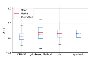
Figure 5: The boxplot displays $\widehat{\beta}-\beta$ over 100 simulations. Our method is displayed as ${\mathsf{DNA\mbox{-}SE}}$, compared to the grid-based method of Zhang & Tchetgen Tchetgen (2022) and the methods using $d$-th degree polynomials, with $d\in\{2,3\}$, respectively displayed as “quadratic” and “cubic” on the horizontal axis of the plot.

We choose $\eta(u,\mathbf{x})=\mathbbm{1}\{u\in[-0.5,0.5]\}$ (defined in Example 3.2) which is completely misspecified compared to the true $\mathrm{p}_{U|\mathbf{X}}(u|\mathbf{x})$. Table 2 displays the numerical estimator of $\widehat{\beta}-\beta^{\ast}$ over 100 simulated datasets obtained from various methods. It is evident that our proposed ${\mathsf{DNA\mbox{-}SE}}$ algorithm is less biased and more efficient compared to polynomials with varying degrees. We also compared ${\mathsf{DNA\mbox{-}SE}}$ with a grid-based method adopted in Zhang & Tchetgen Tchetgen (2022) using their R code; the latter method has longer computation time (about 35 minutes per run) than ${\mathsf{DNA\mbox{-}SE}}$ (below 30 minutes per run) but larger bias and variance. Table 2 provides the summary statistics of the simulation results, supplemented with boxplots in Figure 5 in Appendix E.

Table 2: The table displays the mean and standard error $\widehat{\beta}-\beta^{\ast}$ over 100 simulations. Our method is displayed as ${\mathsf{DNA\mbox{-}SE}}$, compared to the other methods including a grid-based method used in Zhang & Tchetgen Tchetgen (2022) and $d$-th degree polynomial, with $d\in\{2,3\}$, shown as quadratic, cubic in the table.

Mean(std)	${\mathsf{DNA\mbox{-}SE}}$	grid-based method
$\widehat{\beta}-\beta^{\ast}$	0.036(0.155)	0.109(0.426)
Mean(std)	cubic	quadratic
$\widehat{\beta}-\beta^{\ast}$	0.142(0.189)	0.145(0.188)

4.2.3 Example 3.3: Average Loss Estimation in Transfer Learning

Next we apply ${\mathsf{DNA\mbox{-}SE}}$ to the transfer learning problem described in (LABEL:model_data_shift) in Example 3.3. Recall in this problem we are interested in estimating the average target-population loss $\beta^{\ast}$ given in Example 3.3. Here we simply choose $f(x)\equiv\mathrm{expit}(x^{\frac{1}{2}})$ as the prediction function for $Y$, $\phi(x)\equiv x+1$ as the outcome shift mechanism function, and $r_{a}(x)\equiv\pi(x)\equiv x$ as the logit-transformed outcome and data-source conditional expectations. Note that to focus on the main issue of this paper, in the simulation we use the true nuisance parameter $\bm{\eta}$ and related quantities such as $v,h,\cdots$ defined in Example 3.3, without using their estimates. The sample size $N$ is 10000.

The numerical summary statistics of the discrepancies between the estimated parameters, $\widehat{\beta}$, and the true parameters, $\beta^{\ast}$, across 100 simulated datasets are presented in Table 3. The corresponding boxplots, which provide a visual representation of these results, have been relegated to Figure 6. It is evident that our proposed ${\mathsf{DNA\mbox{-}SE}}$ method outperforms the traditional polynomial method with different degrees, in particular in terms of variance (reduced by at least 80%).

Table 3: This table displays $\widehat{\beta}-\beta^{\ast}$ over 100 simulations. Our method is displayed as ${\mathsf{DNA\mbox{-}SE}}$, compared to methods using $d$-th degree polynomials, with $d\in\{5,10,15\}$, respectively displayed as “quintic”, “10th-degree”, “15th-degree” in the table.

Mean(std)	${\mathsf{DNA\mbox{-}SE}}$	quintic
$\widehat{\beta}-\beta^{*}$	-0.0008(0.0084)	0.0009(0.0186)
Mean(std)	10th-degree	15th-degree
$\widehat{\beta}-\beta^{\ast}$	0.0033(0.0234)	0.0038(0.0385)

5 Real Data Application

In this section, we further demonstrate the empirical performance of ${\mathsf{DNA\mbox{-}SE}}$ by reanalyzing a real dataset that was previously analyzed in Zhao & Ma (2022).

5.1 The Connecticut Children’s Mental Health Study

We now apply our proposed ${\mathsf{DNA\mbox{-}SE}}$ algorithm to re-analyze a dataset from a comprehensive investigation conducted by Zahner & Daskalakis (1997) on children’s mental health in Connecticut, USA. This study employed the Achenbach Child Behavior Checklist (CBCL) as a tool to evaluate the psychiatric status of children. The CBCL consists of three different forms, namely parent, teacher, and adolescent self-report. Here the response $Y$ of interest is teacher’s report of the child’s psychiatric status, where $Y=1$ suggests the presence of clinical psychopathology and $Y=0$ suggests normal psychological functioning. In the study, a logistic regression was conducted to examine the relationship between $Y$ and covariates, including $X_{1}$: father’s presence in the household ($X_{1}=1/0$: absence/presence), $X_{2}$: the child’s physical health ($X_{2}=1/0$: poor/good health), $Z$: parent’s report ($Z=1/0$: abnormal/normal clinical psychopathology):

$$\small\mathrm{logit}\ \mathrm{P}(Y=1|Z,X_{1},X_{2})=\beta_{0}+\beta_{1}X_{1}+\beta_{2}X_{2}+\beta_{z}Z,$$

where the regression coefficients $\boldsymbol{\beta}=(\beta_{0},\beta_{1},\beta_{2},\beta_{z})^{\top}$ are the parameters of interest.

This dataset comprises 2486 subjects, of which 1061 (approximately 42.7%) exhibit missing values. The presence of such a large amount of missing data poses a significant challenge, as modeling with only the 1425 subjects with complete data may lead to highly biased estimates for $\boldsymbol{\beta}$. The missingness $A$ of teacher’s report $Y$ is unlikely to be related to the parent’s report $Z$, but $Z$ may be highly correlated with $Y$. Hence $Z$ can be viewed as a so-called “shadow variable” (Miao et al., 2024) to help identify $\boldsymbol{\beta}$ even under MNAR. The semiparametric estimator of $\boldsymbol{\beta}$ leveraging the shadow variable has been derived in Zhao & Ma (2022). A more detailed exposition can be found in Appendix F .

5.2 Data Analysis Results

Besides the estimator computed by ${\mathsf{DNA\mbox{-}SE}}$, for comparison purposes, we also report the results (1) from the observed-only estimator that completely ignores the missing data and (2) from Zhao & Ma (2022) using the algorithm of Atkinson (1967). The observed-only estimator is biased under the MNAR assumption for the regression coefficients of the covariates except $Z$, the shadow variable.

To estimate the standard errors of the ${\mathsf{DNA\mbox{-}SE}}$ estimators of $\boldsymbol{\beta}$, we generate 100 bootstrap samples, each of size 2000, rerun the whole ${\mathsf{DNA\mbox{-}SE}}$ algorithm to obtain the point estimates, and then compute the mean and standard deviation of the point estimates over 100 bootstrap samples. Table 4 displays the point estimates and the estimated standard errors from different methods, including ${\mathsf{DNA\mbox{-}SE}}$, the reported estimates from Table 6 of Zhao & Ma (2022), and the potentially biased observed-only estimates. First, it is reassuring that all three methods produce roughly the same estimate for regression coefficient $\beta_{z}$ of the shadow variable $Z$ (parent’s report), although our method, ${\mathsf{DNA\mbox{-}SE}}$, has the smallest standard error (the 2nd row, 2nd column of Table 4). For the other coefficients, the point estimates of ${\mathsf{DNA\mbox{-}SE}}$ are very close to those from Zhao & Ma (2022) but our (estimated) standard errors of ${\mathsf{DNA\mbox{-}SE}}$ are smaller. Overall, the results of ${\mathsf{DNA\mbox{-}SE}}$ are consistent with that of Zhao & Ma (2022). The “observed-only” approach is more likely to produce biased result due to its stronger yet empirically unverifiable assumption on the missing data mechanism.

Table 4: Comparison of different estimators for $\boldsymbol{\beta}$ in the real data analysis.

Mean(se)	$\widehat{\beta}_{0}$	$\widehat{\beta}_{1}$
${\mathsf{DNA\mbox{-}SE}}$	-1.3289(0.1402)	-0.0623(0.1196)
Zhao & Ma (2022)	-1.3585(0.1823)	-0.0718(0.1470)
observed-only	-1.9307(0.1132)	0.3652(0.1480)
Mean(se)	$\widehat{\beta}_{2}$	$\widehat{\beta}_{z}$
${\mathsf{DNA\mbox{-}SE}}$	-0.6159(0.1366)	1.4620(0.0761)
Zhao & Ma (2022)	-0.9817(0.1320)	1.4623(0.1194)
observed-only	-0.0516(0.1690)	1.4621(0.1583)

6 Concluding Remarks

In this paper, we first proposed a general framework by formulating the semiparametric estimation problem as a bi-level optimization problem; and then we developed a novel algorithm ${\mathsf{DNA\mbox{-}SE}}$ that can simultaneously solve the integral equation and estimate the parameter of interest by employing modern DNN as a numerical solver of the integral equations appeared in the estimation procedure. Compared to traditional approaches, ${\mathsf{DNA\mbox{-}SE}}$ can be scaled to higher-dimensional problems owing to: (1) the universal approximation property (Siegel & Xu, 2020); (2) more efficient optimization algorithms (Kingma & Ba, 2015); and (3) the increasing computing power for deep learning. We also developed a python package that implements the ${\mathsf{DNA\mbox{-}SE}}$ algorithm. In fact, this proposed framework goes beyond semiparametric estimation and can be adapted more broadly to models subject to general moment restrictions in the statistics and econometrics literature (Ai & Chen, 2003; Chen & Santos, 2018).

There are some recent works introducing modern numerical methods, such as methods based on gradient flows (Crucinio et al., 2022) or tensor networks (e.g. tensor train decomposition) (Cichocki et al., 2016, 2017; Corona et al., 2017; Chen et al., 2023b), to the problem of purely solving integral equations. It will be interesting to explore how to incorporate these new generations of numerical toolboxes into semiparametric statistics. Our future plan also includes: (1) providing convergence analysis of Algorithm 1 and possibly supplementing it with consensus-based methods (Carrillo et al., 2021) to accelerate the convergence towards global optimizer in practice; (2) characterizing statistical properties of the obtained estimator; and more importantly, (3) fully automating and “democratizing” semiparametric statistics by eliminating the need of deriving estimators by human, via techniques such as large language models, arithmetic formula learning, differentiable and symbolic computation (Frangakis et al., 2015; Carone et al., 2019; Polu & Sutskever, 2020; Garg et al., 2020; Trinh et al., 2024; Luedtke, 2024).

Impact Statement

The goal of this paper is to advance the field of Machine Learning/Artificial Intelligence by using these tools to boost statistical sciences. There could be many potential positive societal consequences of our work, none of which we feel must be specifically highlighted here.

Appendix A The flow chart of ${\mathsf{DNA\mbox{-}SE}}$

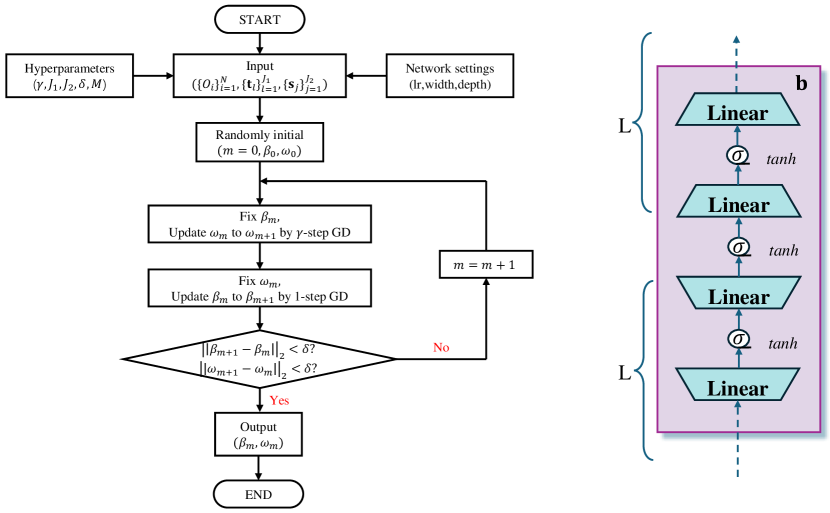
Figure 1: Depicted here is an illustration of our ${\mathsf{DNA\mbox{-}SE}}$ algorithm and the neural network architecture employed for modeling $\mathsf{b}$, the solution to the integral equations. Left: We present a comprehensive flowchart that outlines the algorithmic procedure. Right: The architecture of $\mathsf{b}$ is chosen to be the standard Multilayer Perceptron (MLP) or feedforward neural networks in this paper with tanh activation function. Notably, the MLP is constructed with a depth of $2L+1$, indicating a strategic layering to optimize performance.

Appendix B Further remarks on the loss function (2)

As mentioned in Section 2.2, the (empirical) loss function (2) originates from the following population loss function:

$$\begin{split}&\boldsymbol{\beta}^{\ast}\coloneqq\arg\min_{\boldsymbol{\beta}\in\mathbb{R}^{q}}\mathcal{L}_{\psi}(\boldsymbol{\beta},\mathsf{b}^{\ast})\ \mathrm{s.t.}\ \mathsf{b}^{\ast}(\cdot)\coloneqq\arg\min_{\mathsf{b}\in\mathcal{F}}\mathcal{L}_{K}(\mathsf{b},\boldsymbol{\beta}^{\ast}),\\ &\text{where }\mathcal{L}_{\psi}(\boldsymbol{\beta},\mathsf{b})\coloneqq\left\{\mathrm{E}\left[\psi(O;\mathsf{b}(\cdot),\boldsymbol{\beta})\right]\right\}^{2},\\ &\mathcal{L}_{K}(\mathsf{b})\coloneqq\int_{o}\int_{\mathbf{t}}\left(\int K(\mathbf{s},\mathbf{t},o;\boldsymbol{\beta})\mathsf{b}(\mathbf{s},o)\mathrm{d}\mathbf{s}-C(\mathbf{t},o);\boldsymbol{\beta})-\mathsf{b}(\mathbf{t},o)\right)^{2}\mathrm{d}\nu(\mathbf{t})\mathrm{d}\mathrm{P}(o).\end{split}$$ (9)

We first turn the estimating equation (1) into the above population loss and then replace the integral with respect to $\mathrm{d}\mathrm{P}(o)$ by the empirical average.

We would like to make another remark on this loss function. One can in principle first draw many samples from the space where the parameter of interest $\boldsymbol{\beta}$ lies, and then solve the integral equations over all these possible values. However, the Alternating GD type of algorithms can explore the $\boldsymbol{\beta}$ space more efficiently.

Finally, it is noteworthy that we are interested in the global minimizer of the loss (9). Since the ${\mathsf{DNA\mbox{-}SE}}$ algorithm relies on GD, when multiple local minimizers exist, one could in principle consider a trial-and-error approach and initialize multiple starting points for $\boldsymbol{\beta}$ and the function $\mathsf{b}(\cdot)$ to ensure convergence to the global minimizer. One could also use the idea from consensus-based optimization (Carrillo et al., 2021) by initializing different starting points using Interacting Particle Systems to accelerate the trial-and-error approach by injecting benign correlations among those starting points.

Appendix C Derivations for Section 3

To make our paper relatively self-contained, we provide derivations of the estimators for the examples in Section 3. We want to remark that these derivations are not new and have appeared in the cited works in Section 3.

C.1 Derivations for Example 3.1

From the model given by Example 3.1, the true missing-data mechanism is $\mathrm{P}(A=1|Y=y)=\mathrm{expit}(1+y)$. Given a dataset consisting of $N$ i.i.d. observations $(X_{i},A_{i},A_{i}Y_{i})^{N}_{i=1}$, the observed-data joint likelihood and the observed-data score are given below:

$$\mathrm{p}(x,a,y;\boldsymbol{\beta},\eta)=\mathrm{p}_{X}(x)\left\{\mathrm{p}_{Y|X}(y,x;\boldsymbol{\beta})\mathrm{P}(A=1|Y=y)\right\}^{a}\left\{1-\int\mathrm{p}_{Y|X}(t,x;\boldsymbol{\beta})\mathrm{P}(A=1|Y=t)\mathrm{d}t\right\}^{1-a},$$

$$\mathsf{s}_{\boldsymbol{\beta}}(x,a,ay;\boldsymbol{\beta})=a\frac{\frac{\partial}{\partial\beta}\mathrm{p}_{Y|X}(y,x;\boldsymbol{\beta})}{\mathrm{p}_{Y|X}(y,x;\boldsymbol{\beta})}-(1-a)\frac{\int\frac{\partial}{\partial\boldsymbol{\beta}}\mathrm{p}_{Y|X}(t,x;\boldsymbol{\beta})\mathrm{P}(A=1|Y=t)\mathrm{d}t}{1-\int\mathrm{p}_{Y|X}(t,x;\boldsymbol{\beta})\mathrm{P}(A=1|Y=t)\mathrm{d}t},$$

where $\mathrm{p}_{Y|X}(y,x;\boldsymbol{\beta})$ is assumed to be known up to the parameter value $\boldsymbol{\beta}$, but $\eta$ is completely unknown to the statistician. From semiparametric theory, the nuisance tangent space is $\Lambda=\Lambda_{1}\oplus\Lambda_{2}$, where

$$\Lambda_{1}=\{h(x):\mathrm{E}h(X)=0\},\Lambda_{2} =\left\{ag(y)-(1-a)\frac{\int\mathrm{p}_{Y|X}(t,x;\boldsymbol{\beta})g(t)\eta(t)\mathrm{d}t}{1-\int\mathrm{p}_{Y|X}(t,x;\boldsymbol{\beta})\eta(t)\mathrm{d}t}:\forall\ g(\cdot)\right\}.$$

By definition, one can obtain the observed-data efficient score $\mathsf{s}_{\mathsf{eff},\boldsymbol{\beta}}(x,a,ay)$ with respect to $\boldsymbol{\beta}$ by subtracting from $\mathsf{s}_{\boldsymbol{\beta}}(x,a,ay)$ its projection onto the observed-data nuisance tangent space $\Lambda$. The projection operation leads to the terms involving function $\mathsf{b}(\cdot)$ (corresponding to the function $g$ in $\Lambda_{2}$) in the display below:

$$\mathsf{s}_{\mathsf{eff},\boldsymbol{\beta}}(x,a,ay)=\mathsf{s}_{\boldsymbol{\beta}}(x,a,ay,\boldsymbol{\beta})-a\mathsf{b}(y)+(1-a)\frac{\int\mathrm{p}_{Y\mid X}(t,x;\boldsymbol{\beta})\mathsf{b}(t;\boldsymbol{\beta})\pi(t)\mathrm{d}t}{1-\int\mathrm{p}_{Y\mid X}(t,x;\boldsymbol{\beta})\pi(t)\mathrm{d}t},$$

where $\mathsf{b}(y)$ satisfies the following function:

$$\int\left\{\frac{\partial}{\partial\boldsymbol{\beta}}\mathrm{p}_{Y\mid X}(y,x;\boldsymbol{\beta})+\frac{\int\frac{\partial}{\partial\boldsymbol{\beta}}\mathrm{p}_{Y\mid X}(t,x;\beta)\eta(t)\mathrm{d}t}{\int\mathrm{p}_{Y\mid X}(t,x;\boldsymbol{\beta})(1-\eta(t))\mathrm{d}t}\mathrm{p}_{Y\mid X}(y,x;\boldsymbol{\beta})\right\}\mathrm{p}_{X}(x)\mathrm{d}x$$

$$= \int\left\{\mathsf{b}(y;\boldsymbol{\beta})\mathrm{p}_{Y\mid X}(y,x;\boldsymbol{\beta})+\frac{\int\mathsf{b}(t;\boldsymbol{\beta})\mathrm{p}_{Y\mid X}(t,x;\boldsymbol{\beta})\eta(t)\mathrm{d}t}{\int\mathrm{p}_{Y\mid X}(t,x;\boldsymbol{\beta})(1-\eta(t))\mathrm{d}t}\mathrm{p}_{Y\mid X}(y,x;\boldsymbol{\beta})\right\}\mathrm{p}_{X}(x)\mathrm{d}x.$$

Zhao & Ma (2022) showed that a working model $\eta(y)$ can be used to replace the true missing mechanism $\mathrm{P}(A=1|Y=y)$, which eventually leads to the estimator $\widehat{\boldsymbol{\beta}}$ that solves the following empirical version of the estimating equation:

$$\ \frac{1}{N}\sum_{i=1}^{N}\Bigg{\{}\mathsf{s}_{\boldsymbol{\beta}}\left(X_{i},A_{i},A_{i}Y_{i}\right)-A_{i}\mathsf{b}\left(Y_{i};\boldsymbol{\beta}\right)+\left(1-A_{i}\right)\frac{\int\mathrm{p}_{Y\mid X}\left(t,X_{i};\boldsymbol{\beta}\right)\mathsf{b}(t;\boldsymbol{\beta})\eta(t)\mathrm{d}t}{\int\mathrm{p}_{Y\mid X}(t,X;\boldsymbol{\beta})\left(1-\eta(t)\right)\mathrm{d}t}\Bigg{\}}=0,$$

where

$$\ \frac{1}{N}\sum_{i=1}^{N}\left\{\frac{\partial}{\partial\boldsymbol{\beta}}\mathrm{p}_{Y\mid X}\left(y,X_{i};\boldsymbol{\beta}\right)+\frac{\int\frac{\partial}{\partial\boldsymbol{\beta}}\mathrm{p}_{Y\mid X}\left(t,X_{i};\boldsymbol{\beta}\right)\eta(t)\mathrm{d}t}{\int\mathrm{p}_{Y\mid X}\left(t,X_{i};\boldsymbol{\beta}\right)\left(1-\eta(t)\right)\mathrm{d}t}\mathrm{p}_{Y\mid X}\left(y,X_{i};\boldsymbol{\beta}\right)\right\}$$

$$= \ \frac{1}{N}\sum_{i=1}^{N}\left\{\mathsf{b}(y;\boldsymbol{\beta})\mathrm{p}_{Y\mid X}\left(y,X_{i};\boldsymbol{\beta}\right)+\frac{\int\mathsf{b}(t;\boldsymbol{\beta})\mathrm{p}_{Y\mid X}\left(t,X_{i};\boldsymbol{\beta}\right)\eta(t)\mathrm{d}t}{\int\mathrm{p}_{Y\mid X}\left(t,X_{i};\boldsymbol{\beta}\right)\left(1-\eta(t)\right)\mathrm{d}t}\mathrm{p}_{Y\mid X}\left(y,X_{i};\boldsymbol{\beta}\right)\right\}.$$

Intuitively, this is because one eliminates the information from the nuisance parameters (in particular the guessed model for $A|Y$) in the observed-data efficient score by projecting onto the orthocomplement of the observed-data nuisance tangent space.

C.2 Derivations for Example 3.2

In this example, the likelihood of the complete data can be factorized as follows:

$$\begin{split}\mathrm{p}(\mathbf{X}=\mathbf{x},U=u,A=a,Y=y)=\mathrm{p}_{\mathbf{X}}(\mathbf{x})\mathrm{p}_{U|\mathbf{X}}(u|\mathbf{x})\mathrm{p}_{A|\mathbf{X},U}(a|\mathbf{x},u)\mathrm{p}_{Y|\mathbf{X},U,A}(y|\mathbf{x},u,a;\beta).\end{split}$$

Here the parameter of interest is $\beta$ and the remaining pieces of the joint likelihood are treated as the nuisance parameters $\bm{\eta}$. One can derive the observed-data score with respect to $\beta$ as the conditional expectation of the full-data score with respect to $\beta$: $\mathsf{s}_{\beta}(\mathbf{X},A,Y)=\mathrm{E}\left[\mathsf{s}_{\beta}(\mathbf{X},U,A,Y)|\mathbf{X},A,Y\right]$ (Robins et al., 1994; van der Laan & Robins, 2003). However, one could obtain more efficient estimators which also rely on fewer modeling assumptions by calculating the observed-data efficient score based on $\mathsf{s}_{\beta}(\mathbf{x},a,y)$ as:

$$\mathsf{s}_{\mathsf{eff},\beta}(\mathbf{X},A,Y)\equiv\mathsf{s}_{\beta}(\mathbf{X},A,Y)-\mathrm{E}\left[\mathsf{b}(U,\mathbf{X})\mid\mathbf{X},A,Y\right],$$

where the second term in the above display is simply the projection of $\mathsf{s}_{\beta}(\mathbf{X},A,Y)$ onto the orthocomplement of the observed-data nuisance tangent space $\Lambda$ to be defined later, which further implies that $\mathsf{b}(u,\mathbf{x})$ solves the following the integral equation:

$$\mathrm{E}\left[\mathsf{s}_{\beta}(\mathbf{X},A,Y)\mid\mathbf{X},U\right]=\mathrm{E}\left\{\mathrm{E}[\mathsf{b}(U,\mathbf{X})\mid\mathbf{X},A,Y]\mid\mathbf{X},U\right\}.$$

To derive the observed-data nuisance tangent space, one first obtains the complete-data nuisance tangent space $\Lambda^{F}$:

$$\Lambda^{F}=\Lambda_{1}^{F}\oplus\Lambda_{2}^{F},$$

$$\Lambda_{1}^{F}=\left\{a_{1}(\mathbf{x}):\mathrm{E}\left[a_{1}(\mathbf{X})\right]=0\right\},$$

$$\Lambda_{2}^{F}=\left\{a_{2}(u,\mathbf{x}):\mathrm{E}\left[a_{2}(U,\mathbf{X})\mid\mathbf{X}\right]=0\right\}.$$

It is well-known that the observed-data model tangent space is the expectation of the complete-data model tangent space conditioning on the observed data (Robins et al., 1994; van der Laan & Robins, 2003). Hence the observed-data tangent space $\Lambda$ is:

$$\begin{split}&\Lambda=\Lambda_{1}\oplus\Lambda_{2},\\ &\Lambda_{1}\equiv\mathrm{E}[\Lambda_{1}^{F}|\mathbf{X},A,Y]\equiv\Lambda_{1}^{F}\equiv\left\{a_{1}(\mathbf{x}):\mathrm{E}\left[a_{1}(\mathbf{X})\right]=0\right\},\\ &\Lambda_{2}\equiv\mathrm{E}[\Lambda_{2}^{F}|\mathbf{X},A,Y]\equiv\left\{a_{2}^{\prime}(\mathbf{x},a,y)\equiv\mathrm{E}\left[a_{2}(U,\mathbf{X})\mid\mathbf{X}=\mathbf{x},A=a,Y=y\right]:\mathrm{E}\left[a_{2}(U,\mathbf{X})\mid X\right]=0\right\}.\end{split}$$

Then the projection of $\mathsf{s}_{\beta}(\mathbf{X},A,Y)$ onto $\Lambda$ is simply to find the function $\mathsf{b}(U,\mathbf{X})$ such that $\mathrm{E}[\mathsf{s}_{\beta}(\mathbf{X},A,Y)-\mathrm{E}[\mathsf{b}(U,\mathbf{X})|\mathbf{X},A,Y]|\mathbf{X},U]\equiv 0$ (for this step, see Equation (6) in the online supplementary materials of Zhang & Tchetgen Tchetgen (2022)), which is a Fredholm integral equation of the first kind, an ill-posed problem. However, one can turn this ill-posed problem to a well-posed problem by introducing Tikhonov regularization, which is the route taken in Zhang & Tchetgen Tchetgen (2022).

Since $\mathrm{p}_{U|\mathbf{X}}(u|\mathbf{x})$ cannot be identified from the observed data distribution, one postulate a working model for $\mathrm{p}_{U|\mathbf{X}}(u|\mathbf{x})$ as $\widetilde{\mathrm{p}}(u|\mathbf{x})\coloneqq\eta(u,\mathbf{x})\mathbbm{1}\{u\in[-B,B]\}/2B$ where $B$ is sufficiently large. Thus, under this working model, the integral equation (after Tikhonov regularization by a possibly very small tuning parameter $\lambda$) becomes

$$\int\mathsf{b}^{\ast}(u^{\prime},\mathbf{X})K(u^{\prime},u,\mathbf{X})\mathrm{d}u^{\prime}=C(u,\mathbf{X})-\lambda\mathsf{b}^{\ast}(u,\mathbf{X}).$$

where $C(u,\mathbf{X})$ and $K(u,u^{\prime},\mathbf{X})$ are known functions up to the unknown parameters. In particular, $C(u,\mathbf{X})$ and $K(u^{\prime},u,\mathbf{X})$ are of the forms

$$\begin{split}C(u,\mathbf{X})=&\int\frac{\int\widetilde{\mathsf{s}}_{\beta}(y,a,\mathbf{X},u^{\prime})h(y,a,u^{\prime},\mathbf{X})\mathrm{d}u^{\prime}}{g(y,a,\mathbf{X})}\mathrm{p}_{Y,A|\mathbf{X},U}(y,a|\mathbf{X},u)\mathrm{d}y\mathrm{d}a,\\ K(u^{\prime},u,\mathbf{X})=&\int\frac{\mathrm{p}_{Y,A|\mathbf{X},U}(y,a|\mathbf{X},u^{\prime})\mathrm{p}_{Y,A|\mathbf{X},U}(y,a|\mathbf{X},u)\eta(u^{\prime},\mathbf{X})}{g(y,a,\mathbf{X})}\mathrm{d}y\mathrm{d}a,\end{split}$$

where

$$\begin{split}h(y,a,u^{\prime},\mathbf{X})&=\mathrm{p}_{Y,A|\mathbf{X},U}(y,a|\mathbf{X},u^{\prime})\eta(u^{\prime},\mathbf{X}),\\ g(y,a,\mathbf{X})&=\int\mathrm{p}_{Y,A|\mathbf{X},U}(y,a|\mathbf{X},u^{\prime})\eta(u^{\prime},\mathbf{X})\mathrm{d}u^{\prime}.\end{split}$$

Eventually, one obtains the estimator $\widehat{\beta}$ parameter of interest $\beta$ by solving:

$$0=\frac{1}{N}\sum_{i=1}^{N}\psi(\mathbf{X}_{i},A_{i},Y_{i};\beta),\text{ where }$$

$$\psi(\mathbf{X}_{i},A_{i},Y_{i};\beta)=\frac{\int f(Y_{i},A_{i},\mathbf{X}_{i},u)\mathrm{p}_{Y,A|\mathbf{X},U}(Y_{i},A_{i}|\mathbf{X}_{i},u)\eta(u,\mathbf{X}_{i})\mathrm{d}u}{\int\mathrm{p}_{Y,A|\mathbf{X},U}(Y_{i},A_{i}|\mathbf{X}_{i},u)\eta(u,\mathbf{X}_{i})\mathrm{d}u},$$

$$f(Y_{i},A_{i},\mathbf{X}_{i},u)\coloneqq\widetilde{\mathsf{s}}_{\beta}(Y_{i},A_{i},\mathbf{X}_{i},u)-\mathsf{b}^{\ast}(u,\mathbf{X}_{i}),$$

where we let $\widetilde{\mathrm{p}}(\mathbf{x},u,a,y)$ denote the joint likelihood induced by the working model:

$$\widetilde{\mathrm{p}}(\mathbf{x},u,a,y)=\mathrm{p}_{X}(\mathbf{x})\eta(u,\mathbf{x})\mathrm{p}_{A|\mathbf{X},U}(a|\mathbf{x},u)\mathrm{p}_{Y|\mathbf{X},U,A}(y|\mathbf{x},u,a;\beta)$$

and the score for the working joint law with respect to $\beta$ is simply $\widetilde{\mathsf{s}}_{\beta}(\mathbf{X},U,A,Y)=\frac{\partial\log\widetilde{\mathrm{p}}(\mathbf{X},U,A,Y;\beta)}{\partial\beta}$. Zhang & Tchetgen Tchetgen (2022) showed that even when the working model is completely misspecified, the estimator based on the observed-data efficient score, not the observed-data score, is still consistent. Intuitively, this is because one eliminates the information from the nuisance parameters (in particular the guessed distribution for $U|X$) in the observed-data efficient score by projecting onto the orthocomplement of the observed-data nuisance tangent space. Proof details are provided in Zhang & Tchetgen Tchetgen (2022) for the aforementioned equations.

C.3 Derivations for Example 3.3

In the example of target-population average loss estimation in the context of transfer learning, the main structural assumption of Qiu et al. (2023) is the following relationship of the logit conditional outcome models between the target ($A=0$) and the source ($A=1$) population: let $\phi:\mathbb{R}\rightarrow\mathbb{R}$ be a strictly increasing function with non-zero first derivative, and Qiu et al. (2023) impose the following:

$$\mathrm{logit}\ \mathrm{P}(Y=1|X=x,A=1)=\phi\left(\mathrm{logit}\ \mathrm{P}(Y=1|X=x,A=0)\right).$$ (10)

As mentioned in the main text, the parameter of interest is the average squared-error loss of prediction $Y$ using a (possibly arbitrary) prediction function $f(\cdot)$ in the target population (i.e. conditioning on $A=0$):

$$\begin{split}\beta^{*}&\coloneqq\mathrm{E}[\ell(X,Y)|A=0],\text{ where }\ell(x,y)=(y-f(x))^{2}.\end{split}$$

The full derivation of the semiparametric efficient estimator $\widehat{\beta}$ can be found in Section S9.6 of Qiu et al. (2023). But we recapture the main idea here for readers’ convenience. To avoid clutter, we do not repeat the definitions of the notation already appeared in Example 3.3. Similar to the above two examples, the derivation starts from the observed-data joint likelihood:

$$\mathrm{p}(X=x,A=a,Y=y)= \ \mathrm{p}_{X}(x)\mathrm{p}_{A|X}(a|x)\mathrm{P}(Y=1|X=x,A=1)^{ay}\mathrm{P}(Y=0|X=x,A=1)^{a(1-y)}$$

$$\times\mathrm{P}(Y=1|X=x,A=0)^{(1-a)y}\mathrm{P}(Y=0|X=x,A=0)^{(1-a)(1-y)}$$

$$= \ \mathrm{p}_{X}(x)\mathrm{p}_{A|X}(a|x)\{\mathrm{expit}\circ\phi\circ r_{0}(x)\}^{ay}\{1-\mathrm{expit}\circ\phi\circ r_{0}(x)\}^{a(1-y)}$$

$$\times\{\mathrm{expit}\circ r_{0}(x)\}^{(1-a)y}\{1-\mathrm{expit}\circ r_{0}(x)\}^{(1-a)(1-y)}.$$

In this example, since the parameter of interest $\beta^{\ast}$ and the nuisance parameters are not in separate pieces of the joint likelihood decomposition, one needs to first derive one influence function $\mathsf{IF}$ of $\beta^{\ast}$ (a mean-zero random variable that is the functional first-order derivative of $\beta^{\ast}$ (van der Vaart, 2002)), then characterize the model tangent space $\mathcal{T}$, and finally obtain the efficient influence function $\mathsf{EIF}$ of $\beta^{\ast}$ by projecting $\mathsf{IF}$ onto the model tangent space $\mathcal{T}$ (van der Laan & Robins, 2003; Tsiatis, 2007).

First, one can easily obtain one influence function of $\beta^{\ast}$ following standard functional differentiation argument recently reviewed in Hines et al. (2022):

$$\mathsf{IF}=\frac{1-A}{\mathrm{P}(A=0)}(\ell(X,Y)-\beta^{\ast}).$$

The model tangent space $\mathcal{T}$ under constraint (10) can be derived from the observed-data joint likelihood as the closure of the direct sum of the space of all scores with respect to each piece of the joint likelihood. Here since one does not model the joint likelihood parametrically, the score with respect to each piece is defined via paths of parametric submodels that go through the underlying likelihood; for details, see van der Vaart (2002) or Section S9.6 of Qiu et al. (2023). With constraint like (10), it is often easier to derive the orthocomplement $\mathcal{T}^{\perp}$ of $\mathcal{T}$. In particular, Qiu et al. (2023) showed the following:

$$\mathcal{T}^{\perp}\equiv\left\{\begin{array}[]{c}A(Y-\mathrm{expit}\circ\phi\circ r_{0}(X))f(X)-(1-A)(Y-\mathrm{expit}\circ r_{0}(X))\frac{h(X,1)\cdot\phi^{\prime}\circ r_{0}(X)}{h(X,0)}f(X):\\ \forall\ f\ \mathrm{s.t.}\ \mathrm{E}[h(X,1)f(X)|r_{0}(X)]\equiv 0\end{array}\right\}.$$

With $\mathcal{T}^{\perp}$, one can obtain $\mathsf{EIF}$ by subtracting from $\mathsf{IF}$ the projection of $\mathsf{IF}$ onto $\mathcal{T}^{\perp}$ to obtain the final semiparametric efficient estimator $\widehat{\beta}$. In particular, this projection operation in order to determine the unique $f\equiv\mathsf{b}^{\ast}$ in $\mathcal{T}^{\perp}$ leads to the following integral equation:

$$\int_{x^{\prime}\in\mathcal{S}(x)}\mathsf{b}^{\ast}(x^{\prime})\frac{v(x^{\prime};1)}{\mu(x^{\prime})}\mathrm{p}_{X}(x^{\prime})\mathrm{d}x^{\prime}+C(x)=\mathsf{b}^{\ast}(x).$$

where $\mathcal{S}(x)=\{x^{\prime}:r_{0}(x^{\prime})=r_{0}(x)\}$ and the definition of $C$ can be found in Example 3.3 (with all the $\widehat{\cdot}$ removed in $\widehat{C}$). As in the main text, let:

$$\mathscr{A}g(x)=\int_{x^{\prime}\in\mathcal{S}(x)}g(x^{\prime})\frac{v(x^{\prime};1)}{\mu(x^{\prime})}\mathrm{p}_{X}(x^{\prime})\mathrm{d}x^{\prime}.$$

The efficient influence function $\mathsf{EIF}$ for $\beta^{*}$ is then

$$\mathsf{EIF}=\frac{1-A}{\mathrm{P}(A=0)}(v(X)-\beta^{\ast})+A(Y-\mathrm{expit}\circ\phi\circ r_{0}(X))g_{1}(X)+(1-A)(Y-\mathrm{expit}\circ r_{0}(X))g_{2}(X),$$

with $g_{1},g_{2}$ defined as in the main text, except removing all the $\widehat{\cdot}$.

Appendix D Hyperparameter tuning

The tuning parameters that vary the most include the width and depth of the network, as well as the alternating frequency $\gamma$. Through grid search and 5-fold cross-validation, for MNAR, the optimal network width and depth are 5 and 3, respectively, resulting in the lowest average MSE. Conversely, in the sensitivity analysis, the optimal network width and depth are 33 and 23, respectively. In the case of transfer learning, which differs from the other two examples in that the integral equations do not depend on the parameter of interest $\boldsymbol{\beta}$, the optimal width and depth are 5 and 3. The effect of different choices of $\gamma$ is depicted in Figure 2 and 3. In all the examples, we choose the activation function as $\mathsf{tanh}$, which is more commonly used in DNN for problems in scientific computing (Lu et al., 2022). We choose the Monte Carlo sample sizes $J_{1}$ and $J_{2}$ to be 1000.

D.1 Hyperparameter tuning for Example 3.1

We find that in this example the alternating frequency $\gamma$ heavily affects the speed and stability of convergence, for the detail see Figure 2. When $\gamma$ is set to 1, i.e. when the neuron parameters $\omega$ and the target parameter $\beta$ are updated in every other iteration, the training process fails to converge and oscillates with extremely high frequency (not shown in Figure 2). When we increases $\gamma$, the training process starts to stabilize after a certain number of iterations and ${\mathsf{DNA\mbox{-}SE}}$ eventually outputs $\widehat{\boldsymbol{\beta}}\approx\boldsymbol{\beta}=(0.25,-0.5)^{\top}$ (Figure 2). However, there exists a trade-off: when $\gamma=5$, the training process converges steeply but also exhibits some instability as the iteration continues; whereas when $\gamma=20$, it takes much longer time for the training process to converge. For the time being, we recommend practitioners try multiple $\gamma$’s (higher than 5) and check if they all eventually converge to the same values. It is an interesting research problem to study an adaptive procedure of choosing $\gamma_{\mathsf{opt}}$ that optimally balances speed and stability of the training. Finally, we found that the results are not sensitive to the Monte Carlo sample sizes $J_{1},J_{2}$ as long as they are sufficiently large.

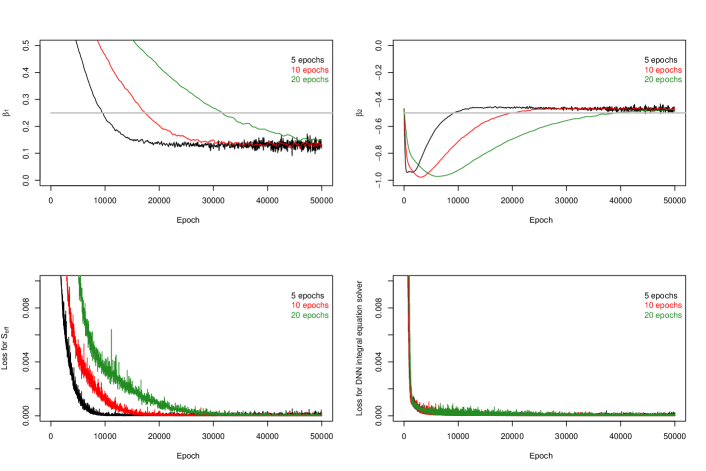
Figure 2: The evolution of training processes in one simulated dataset of Example 4.2.1 by setting the alternating frequency $\gamma$ as $5,10$, or $20$. The horizontal axis is the number of iterations. The upper panels show the evolution of $\beta_{1}$ (left) and $\beta_{2}$ (right) over iterations, while the lower panels show the evolution of the loss corresponding to the score equation (left) and the integral equation (right) over iterations.

D.2 Hyperparameter tuning for Example 3.2

Similar to the last example, it is imperative to examine whether various alternating frequencies will impact the outcomes. However, in contrast to Example 3.1, all training processes stabilize at different rates that are directly proportional to the alternating frequency. The tuning details for simulations described in Section 4.2.2 are presented in Figure 3. The depicted figure provides a comprehensive analysis of the alternate frequencies $\gamma$ employed, namely 1, 5, 10, and 20, revealing their performance similarities. Notably, the convergence rate appears to be faster when $\gamma$ is set to 1, as observed from the figure. For the regularization parameter $\lambda$, we simply choose $\lambda=0.001$ in this paper.

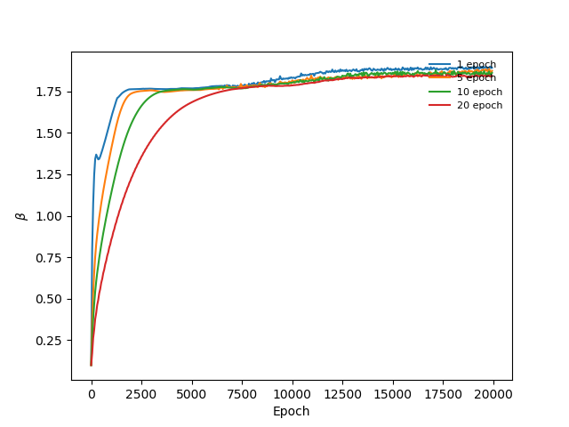
(a)

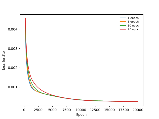
(b)

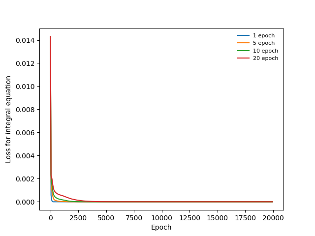
(c)

Figure 3: The evolution of training processes in one simulated dataset of Example 4.2.2 by setting the alternating frequency $\gamma$ as $1,5,10$, or $20$. The horizontal axis is the number of iterations. The upper panels show the evolution of (a) $\beta$ over iterations, while the lower panels show the evolution of the loss corresponding to (b) the score equation and (c) the integral equation over iterations.

D.3 Hyperparameter tuning for Example 3.3

Compared to the two previous examples, the main distinctive feature of this example is that the integral equation does not depend on the parameter of interest $\beta$. Thus in this special case, there is no need to use Alternating GD type of algorithms and regular GD type of algorithms suffices. As a result, there is no need to tune the alternating frequency $\gamma$ in Algorithm 1.

Appendix E Supplementary figures for Section 4

This section collects supplementary figures (Figures 4 to 5) for the numerical experiments that were only referenced in Section 4 due to space limitation.

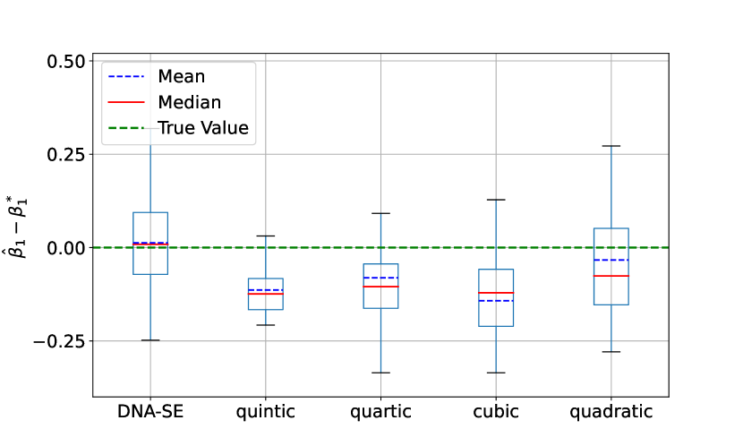
(a)

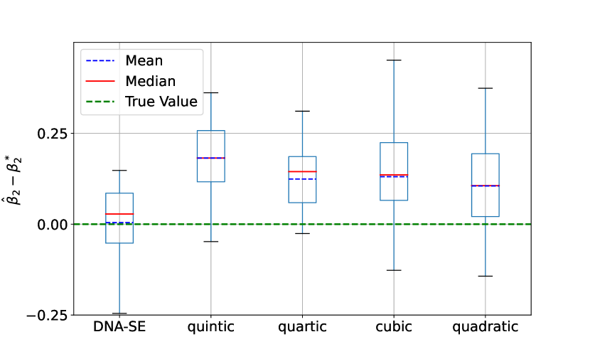
(b)

Figure 4: The boxplots of (a) and (b) display $\widehat{\beta}_{1}-\beta_{1}$ and $\widehat{\beta}_{2}-\beta_{2}$ over 100 simulations. Our method is displayed as ${\mathsf{DNA\mbox{-}SE}}$, compared to the methods using $d$-th degree polynomials, with $d\in\{2,3,4,5\}$, respectively displayed as “quadratic”, “cubic”, “quartic”, and “quintic” on the horizontal axis of the plot.

Figure 6: The boxplot displays $\widehat{\beta}-\beta^{\ast}$ over 100 simulations. Our method is displayed as ${\mathsf{DNA\mbox{-}SE}}$, compared to methods using $d$-th degree polynomials, with $d\in\{5,10,15\}$, respectively displayed as “quintic”, “10th-degree”, “15th-degree” on the horizontal axis of the plot.

Appendix F The estimators used for real data analysis

Following Zhao & Ma (2022), the missing data mechanism is posited to be $\eta^{\ast}(Y,X_{1},X_{2})$, as a function of the response teacher’s report, covariates $X_{1}$ (father’s presence) and $X_{2}$ (child’s health):

$$\begin{split}&\ \eta^{\ast}(Y,X_{1},X_{2})=\mathrm{logit}\ \mathrm{P}(A=1|Y,X_{1},X_{2})=1.058-2.037Y-0.002X_{1}+0.298X_{2}.\end{split}$$

Zhao & Ma (2022) also posited the following model for the shadow variable $Z$, as:

$$\begin{split}&\ \mathrm{logit}\ \mathrm{P}(Z=1|X_{1},X_{2})=-2.106+0.623X_{1}+0.890X_{2}.\end{split}$$

The parameters of interest are $\boldsymbol{\beta}=(\beta_{0},\beta_{1},\beta_{2},\beta_{z})^{\top}$ and the estimator $\widehat{\boldsymbol{\beta}}$ is given below:

$$\begin{split}\widehat{\boldsymbol{\beta}}=&\arg\min_{\boldsymbol{\beta}\in\mathbb{R}^{2}}\left\{\frac{1}{N}\sum_{i=1}^{N}\psi(\mathbf{X}_{i},Z_{i},Y_{i},A_{i};\boldsymbol{\beta},\widehat{\mathsf{b}})\right\}^{2},\text{where}\\ \widehat{\mathsf{b}}=&\arg\min_{\mathsf{b}}\frac{1}{N}\sum_{i=1}^{N}\int_{t}\Bigg{(}\int\mathsf{b}(s,\mathbf{x})K(s,t,\mathbf{x},\mathbf{X}_{i},Z_{i};\widehat{\boldsymbol{\beta}})\mathrm{d}s-C(t,\mathbf{x},Z_{i};\widehat{\boldsymbol{\beta}})-\mathrm{p}_{Y|\mathbf{X},Z}(t|\mathbf{x},Z_{i};\widehat{\boldsymbol{\beta}})\mathsf{b}(t,\mathbf{x})\Bigg{)}^{2}\mathrm{d}\nu(t).\end{split}$$

Here,

$$\psi(\mathbf{X}_{i},Z_{i},A_{i},Y_{i},\boldsymbol{\beta},\mathsf{b})=\frac{1}{N}\sum_{i=1}^{N}\Bigg{\{}A_{i}\frac{\frac{\partial}{\partial\boldsymbol{\beta}}\mathrm{p}_{Y|\mathbf{X},Z}(Y_{i}|\mathbf{X}_{i},Z_{i};\boldsymbol{\beta})}{\mathrm{p}_{Y|\mathbf{X},Z}(Y_{i}|\mathbf{X}_{i},Z_{i};\boldsymbol{\beta})}-A_{i}\mathsf{b}(Y_{i},\mathbf{X}_{i})$$

$$-(1-A_{i})\frac{\int\frac{\partial}{\partial\boldsymbol{\beta}}\mathrm{p}_{Y|\mathbf{X},Z}(Y_{i}|\mathbf{X}_{i},Z_{i};\boldsymbol{\beta})\eta^{\ast}(t)\mathrm{d}t}{\int\mathrm{p}_{Y|\mathbf{X},Z}(t|\mathbf{X}_{i},Z_{i};\boldsymbol{\beta})(1-\eta^{\ast}(t))\mathrm{d}t}+\ (1-A_{i})\frac{\int\mathrm{p}_{Y|\mathbf{X},Z}(t|\mathbf{X}_{i},Z_{i};\boldsymbol{\beta})\mathsf{b}(t,\mathbf{X}_{i})\eta^{\ast}(t)\mathrm{d}t}{\int\mathrm{p}_{Y|\mathbf{X},Z}(t|\mathbf{X}_{i},Z_{i};\boldsymbol{\beta})(1-\eta^{\ast}(t))\mathrm{d}t}\Bigg{\}},$$

and $C(\cdot)$ and $K(\cdot)$ are defined as follows:

$$\begin{split}&C(t,\mathbf{x},Z_{i};\boldsymbol{\beta})\equiv\frac{\partial}{\partial\boldsymbol{\beta}}\mathrm{p}_{Y|\mathbf{X},Z}(t|\mathbf{x},Z_{i};\boldsymbol{\beta})+\frac{\int\frac{\partial}{\partial\boldsymbol{\beta}}\mathrm{p}_{Y|\mathbf{X},Z}(s|\mathbf{x},Z_{i};\boldsymbol{\beta})\eta^{\ast}(s)\mathrm{d}s}{\int\mathrm{p}_{Y|X}(s,\mathbf{x},Z_{i};\boldsymbol{\beta})(1-\eta^{\ast}(s))\mathrm{d}s}\mathrm{p}_{Y|X}(t,\mathbf{x},Z_{i};\boldsymbol{\beta}),\\ &K(s,t,\mathbf{x},\mathbf{X}_{i},Z_{i};\boldsymbol{\beta})\equiv\frac{\mathrm{p}_{Y|\mathbf{X},Z}(s|\mathbf{x},Z_{i};\boldsymbol{\beta})\mathrm{p}_{Y|\mathbf{X},Z}(t|\mathbf{x},Z_{i};\boldsymbol{\beta})\eta^{\ast}(s)}{\int\mathrm{p}_{Y|\mathbf{X},Z}(s^{\prime}|\mathbf{x},Z_{i};\boldsymbol{\beta})(1-\eta^{\ast}(s^{\prime}))\mathrm{d}s^{\prime}}\text{Kernel}_{h}(\mathbf{X}_{i}-\mathbf{x}).\end{split}$$

Here $\text{Kernel}_{h}(\cdot)\coloneqq\text{Kernel}(\cdot/h)/h$ and the kernel function is chosen based on the criteria outlined in Section 4 of Zhao & Ma (2022). In the simulation, we choose the same kernel function as in Zhao & Ma (2022) with the same bandwidth $h=3N^{-1/5}$:

$$\text{Kernel}(t)=\frac{45}{32}\left(1-\frac{7}{3}t^{2}\right)\left(1-t^{2}\right)I_{\{|t|\leq 1\}}.$$

References

- Ai & Chen (2003) Ai, C. and Chen, X. Efficient estimation of models with conditional moment restrictions containing unknown functions. Econometrica, 71(6):1795–1843, 2003.
- Atkinson (1967) Atkinson, K. E. The numerical solution of Fredholm integral equations of the second kind. SIAM Journal on Numerical Analysis, 4(3):337–348, 1967.
- Bellour et al. (2016) Bellour, A., Sbibih, D., and Zidna, A. Two cubic spline methods for solving Fredholm integral equations. Applied Mathematics and Computation, 276:1–11, 2016.
- Bickel et al. (1998) Bickel, P. J., Klaassen, C. A. J., Ritov, Y., and Wellner, J. A. Efficient and Adaptive Estimation for Semiparametric Models. Johns Hopkins Series in the Mathematical Sciences. Springer New York, 1998. ISBN 9780387984735.
- Carone et al. (2019) Carone, M., Luedtke, A. R., and van der Laan, M. J. Toward computerized efficient estimation in infinite-dimensional models. Journal of the American Statistical Association, 114(527):1174–1190, 2019.
- Carrillo et al. (2021) Carrillo, J. A., Jin, S., Li, L., and Zhu, Y. A consensus-based global optimization method for high dimensional machine learning problems. ESAIM: Control, Optimisation and Calculus of Variations, 27:S5, 2021.
- Chen et al. (2023a) Chen, J., Chen, X., and Tamer, E. Efficient estimation of average derivatives in NPIV models: Simulation comparisons of neural network estimators. Journal of Econometrics, 235(2):1848–1875, 2023a.
- Chen et al. (2023b) Chen, S., Li, J., Li, Y., and Zhang, A. R. Learning polynomial transformations via generalized tensor decompositions. In Proceedings of the 55th Annual ACM Symposium on Theory of Computing, pp. 1671–1684, 2023b.
- Chen et al. (2021) Chen, T., Sun, Y., and Yin, W. Closing the gap: Tighter analysis of alternating stochastic gradient methods for bilevel problems. Advances in Neural Information Processing Systems, 34:25294–25307, 2021.
- Chen & Santos (2018) Chen, X. and Santos, A. Overidentification in regular models. Econometrica, 86(5):1771–1817, 2018.
- Chen & White (1999) Chen, X. and White, H. Improved rates and asymptotic normality for nonparametric neural network estimators. IEEE Transactions on Information Theory, 45(2):682–691, 1999.
- Chen et al. (2024) Chen, X., Liu, Y., Ma, S., and Zhang, Z. Causal inference of general treatment effects using neural networks with a diverging number of confounders. Journal of Econometrics, 238(1):105555, 2024.
- Chernozhukov et al. (2018) Chernozhukov, V., Chetverikov, D., Demirer, M., Duflo, E., Hansen, C., Newey, W., and Robins, J. Double/debiased machine learning for treatment and structural parameters. The Econometrics Journal, 21(1):C1–C68, 2018.
- Chernozhukov et al. (2022) Chernozhukov, V., Newey, W., Quintas-Martınez, V. M., and Syrgkanis, V. RieszNet and ForestRiesz: Automatic debiased machine learning with neural nets and random forests. In International Conference on Machine Learning, pp. 3901–3914. PMLR, 2022.
- Cichocki et al. (2016) Cichocki, A., Lee, N., Oseledets, I., Phan, A.-H., Zhao, Q., and Mandic, D. P. Tensor networks for dimensionality reduction and large-scale optimization: Part 1 low-rank tensor decompositions. Foundations and Trends® in Machine Learning, 9(4-5):249–429, 2016.
- Cichocki et al. (2017) Cichocki, A., Phan, A.-H., Zhao, Q., Lee, N., Oseledets, I., Sugiyama, M., and Mandic, D. P. Tensor networks for dimensionality reduction and large-scale optimization: Part 2 applications and future perspectives. Foundations and Trends® in Machine Learning, 9(6):431–673, 2017.
- Corona et al. (2017) Corona, E., Rahimian, A., and Zorin, D. A tensor-train accelerated solver for integral equations in complex geometries. Journal of Computational Physics, 334:145–169, 2017.
- Crucinio et al. (2022) Crucinio, F. R., De Bortoli, V., Doucet, A., and Johansen, A. M. Solving Fredholm integral equations of the first kind via Wasserstein gradient flows. arXiv preprint arXiv:2209.09936, 2022.
- Cui et al. (2023) Cui, Y., Pu, H., Shi, X., Miao, W., and Tchetgen Tchetgen, E. Semiparametric proximal causal inference. Journal of the American Statistical Association, 2023.
- E & Yu (2018) E, W. and Yu, B. The deep Ritz method: a deep learning-based numerical algorithm for solving variational problems. Communications in Mathematics and Statistics, 6(1):1–12, 2018.
- Farrell et al. (2021) Farrell, M. H., Liang, T., and Misra, S. Deep neural networks for estimation and inference. Econometrica, 89(1):181–213, 2021.
- Finn et al. (2017) Finn, C., Abbeel, P., and Levine, S. Model-agnostic meta-learning for fast adaptation of deep networks. In International Conference on Machine Learning, pp. 1126–1135. PMLR, 2017.
- Frangakis et al. (2015) Frangakis, C. E., Qian, T., Wu, Z., and Diaz, I. Deductive derivation and Turing-computerization of semiparametric efficient estimation. Biometrics, 71(4):867–874, 2015.
- Garg et al. (2020) Garg, A., Kayal, N., and Saha, C. Learning sums of powers of low-degree polynomials in the non-degenerate case. In 2020 IEEE 61st Annual Symposium on Foundations of Computer Science (FOCS), pp. 889–899. IEEE, 2020.
- Giné & Nickl (2016) Giné, E. and Nickl, R. Mathematical foundations of infinite-dimensional statistical models, volume 40. Cambridge University Press, 2016.
- Goel et al. (2020) Goel, S., Gollakota, A., Jin, Z., Karmalkar, S., and Klivans, A. Superpolynomial lower bounds for learning one-layer neural networks using gradient descent. In International Conference on Machine Learning, pp. 3587–3596. PMLR, 2020.
- Gong et al. (2016) Gong, M., Zhang, K., Liu, T., Tao, D., Glymour, C., and Schölkopf, B. Domain adaptation with conditional transferable components. In International Conference on Machine Learning, pp. 2839–2848. PMLR, 2016.
- Guan et al. (2022) Guan, Y., Fang, T., Zhang, D., and Jin, C. Solving Fredholm integral equations using deep learning. International Journal of Applied and Computational Mathematics, 8(2):87, 2022.
- Hines et al. (2022) Hines, O., Dukes, O., Diaz-Ordaz, K., and Vansteelandt, S. Demystifying statistical learning based on efficient influence functions. The American Statistician, 76(3):292–304, 2022.
- Kingma & Ba (2015) Kingma, D. P. and Ba, J. L. Adam: A method for stochastic optimization. In International Conference on Learning Representations, 2015.
- Kompa et al. (2022) Kompa, B., Bellamy, D., Kolokotrones, T., Robins, J. M., and Beam, A. Deep learning methods for proximal inference via maximum moment restriction. In Proceedings of the 36th International Conference on Neural Information Processing Systems, pp. 11189–11201, 2022.
- Krizhevsky et al. (2012) Krizhevsky, A., Sutskever, I., and Hinton, G. E. ImageNet classification with deep convolutional neural networks. In Proceedings of the 25th International Conference on Neural Information Processing Systems, pp. 1097–1105, 2012.
- Lee et al. (2023) Lee, J. J., Bhattacharya, R., Nabi, R., and Shpitser, I. Ananke: A python package for causal inference using graphical models. arXiv preprint arXiv:2301.11477, 2023.
- Li et al. (2020) Li, X.-A., Xu, Z.-Q. J., and Zhang, L. A multi-scale DNN algorithm for nonlinear elliptic equations with multiple scales. Communications in Computational Physics, 28(5):1886–1906, 2020.
- Li et al. (2023) Li, Z., Cai, R., Chen, G., Sun, B., Hao, Z., and Zhang, K. Subspace identification for multi-source domain adaptation. In Advances in Neural Information Processing Systems, volume 36, 2023.
- Liang (2021) Liang, T. How well generative adversarial networks learn distributions. Journal of Machine Learning Research, 22(228):1–41, 2021.
- Liu (2001) Liu, J. S. Monte Carlo strategies in scientific computing, volume 75. Springer, 2001.
- Liu et al. (2021a) Liu, L., Shahn, Z., Robins, J. M., and Rotnitzky, A. Efficient estimation of optimal regimes under a no direct effect assumption. Journal of the American Statistical Association, 116(533):224–239, 2021a.
- Liu et al. (2021b) Liu, Q., Xu, J., Jiang, R., and Wong, W. H. Density estimation using deep generative neural networks. Proceedings of the National Academy of Sciences, 118(15):e2101344118, 2021b.
- Lu et al. (2022) Lu, Y., Chen, H., Lu, J., Ying, L., and Blanchet, J. Machine learning for elliptic PDEs: Fast rate generalization bound, neural scaling law and minimax optimality. In International Conference on Learning Representations, 2022.
- Luedtke (2024) Luedtke, A. Simplifying debiased inference via automatic differentiation and probabilistic programming. arXiv preprint arXiv:2405.08675, 2024.
- Miao et al. (2024) Miao, W., Liu, L., Li, Y., Tchetgen Tchetgen, E. J., and Geng, Z. Identification and semiparametric efficiency theory of nonignorable missing data with a shadow variable. ACM/JMS Journal of Data Science, 1(2):1–23, 2024.
- Min et al. (2023) Min, S., Shi, W., Lewis, M., Chen, X., Yih, W.-t., Hajishirzi, H., and Zettlemoyer, L. Nonparametric masked language modeling. In Findings of the Association for Computational Linguistics: ACL 2023, pp. 2097–2118, 2023.
- Newey (1990) Newey, W. K. Semiparametric efficiency bounds. Journal of Applied Econometrics, 5(2):99–135, 1990.
- Neyshabur (2017) Neyshabur, B. Implicit regularization in deep learning. PhD thesis, Toyota Technological Institute at Chicago (TTIC), 2017.
- Padilla et al. (2022) Padilla, O. H. M., Tansey, W., and Chen, Y. Quantile regression with ReLU networks: Estimators and minimax rates. Journal of Machine Learning Research, 23(247):1–42, 2022.
- Pan et al. (2022) Pan, X., Yao, W., Zhang, H., Yu, D., Yu, D., and Chen, J. Knowledge-in-context: Towards knowledgeable semi-parametric language models. In International Conference on Learning Representations, 2022.
- Polu & Sutskever (2020) Polu, S. and Sutskever, I. Generative language modeling for automated theorem proving. arXiv preprint arXiv:2009.03393, 2020.
- Qiu et al. (2023) Qiu, H., Tchetgen, E. T., and Dobriban, E. Efficient and multiply robust risk estimation under general forms of dataset shift. arXiv preprint arXiv:2306.16406, 2023.
- Raissi et al. (2019) Raissi, M., Perdikaris, P., and Karniadakis, G. E. Physics-informed neural networks: A deep learning framework for solving forward and inverse problems involving nonlinear partial differential equations. Journal of Computational Physics, 378:686–707, 2019.
- Ren et al. (1999) Ren, Y., Zhang, B., and Qiao, H. A simple Taylor-series expansion method for a class of second kind integral equations. Journal of Computational and Applied Mathematics, 110(1):15–24, 1999.
- Robins et al. (1994) Robins, J. M., Rotnitzky, A., and Zhao, L. P. Estimation of regression coefficients when some regressors are not always observed. Journal of the American Statistical Association, 89(427):846–866, 1994.
- Robins et al. (2000) Robins, J. M., Rotnitzky, A., and Scharfstein, D. O. Sensitivity analysis for selection bias and unmeasured confounding in missing data and causal inference models. In Statistical Models in Epidemiology, the Environment, and Clinical Trials, pp. 1–94. Springer, 2000.
- Schmidt-Hieber (2020) Schmidt-Hieber, J. Nonparametric regression using deep neural networks with ReLU activation function. Annals of Statistics, 48(4):1875–1897, 2020.
- Scott (2019) Scott, C. A generalized Neyman-Pearson criterion for optimal domain adaptation. In Algorithmic Learning Theory, pp. 738–761. PMLR, 2019.
- Shi et al. (2021) Shi, C., Xu, T., Bergsma, W., and Li, L. Double generative adversarial networks for conditional independence testing. Journal of Machine Learning Research, 22(285):1–32, 2021.
- Siegel & Xu (2020) Siegel, J. W. and Xu, J. Approximation rates for neural networks with general activation functions. Neural Networks, 128:313–321, 2020.
- Suzuki (2019) Suzuki, T. Adaptivity of deep ReLU network for learning in Besov and mixed smooth Besov spaces: optimal rate and curse of dimensionality. In International Conference on Learning Representations, 2019.
- Tian et al. (2023) Tian, Q., Zhang, X., and Zhao, J. ELSA: Efficient label shift adaptation through the lens of semiparametric models. In International Conference on Machine Learning, pp. 34120–34142. PMLR, 2023.
- Trinh et al. (2024) Trinh, T. H., Wu, Y., Le, Q. V., He, H., and Luong, T. Solving olympiad geometry without human demonstrations. Nature, 625(7995):476–482, 2024.
- Tsiatis (2007) Tsiatis, A. Semiparametric theory and missing data. Springer Science & Business Media, 2007.
- van der Laan & Robins (2003) van der Laan, M. J. and Robins, J. M. Unified methods for censored longitudinal data and causality. Springer Science & Business Media, 2003.
- van der Vaart (2002) van der Vaart, A. Part III: Semiparameric statistics. Lectures on Probability Theory and Statistics, pp. 331–457, 2002.
- van der Vaart & Wellner (2023) van der Vaart, A. W. and Wellner, J. Weak Convergence and Empirical Processes: with Applications to Statistics. Springer Science & Business Media, 2023.
- Vaswani et al. (2017) Vaswani, A., Shazeer, N., Parmar, N., Uszkoreit, J., Jones, L., Gomez, A. N., Kaiser, Ł., and Polosukhin, I. Attention is all you need. In Proceedings of the 31st International Conference on Neural Information Processing Systems, pp. 6000–6010, 2017.
- Vempala & Wilmes (2019) Vempala, S. and Wilmes, J. Gradient descent for one-hidden-layer neural networks: Polynomial convergence and SQ lower bounds. In Conference on Learning Theory, pp. 3115–3117. PMLR, 2019.
- Wang et al. (2023) Wang, H., Fu, T., Du, Y., Gao, W., Huang, K., Liu, Z., Chandak, P., Liu, S., Van Katwyk, P., Deac, A., et al. Scientific discovery in the age of artificial intelligence. Nature, 620(7972):47–60, 2023.
- Wilson et al. (2017) Wilson, A. C., Roelofs, R., Stern, M., Srebro, N., and Recht, B. The marginal value of adaptive gradient methods in machine learning. In Proceedings of the 31st International Conference on Neural Information Processing Systems, pp. 4151–4161, 2017.
- Xu et al. (2022) Xu, S., Liu, L., and Liu, Z. DeepMed: Semiparametric causal mediation analysis with debiased deep learning. In Proceedings of the 36th International Conference on Neural Information Processing Systems, pp. 28238–28251, 2022.
- Yang (2022) Yang, S. Semiparametric estimation of structural nested mean models with irregularly spaced longitudinal observations. Biometrics, 78(3):937–949, 2022.
- Zahner & Daskalakis (1997) Zahner, G. E. and Daskalakis, C. Factors associated with mental health, general health, and school-based service use for child psychopathology. American Journal of Public Health, 87(9):1440–1448, 1997.
- Zappala et al. (2023) Zappala, E., Fonseca, A. H. d. O., Moberly, A. H., Higley, M. J., Abdallah, C., Cardin, J. A., and van Dijk, D. Neural integro-differential equations. In Proceedings of the AAAI Conference on Artificial Intelligence, volume 37 (9), pp. 11104–11112, 2023.
- Zhang & Tchetgen Tchetgen (2022) Zhang, B. and Tchetgen Tchetgen, E. J. A semi-parametric approach to model-based sensitivity analysis in observational studies. Journal of the Royal Statistical Society Series A: Statistics in Society, 185(Supplement_2):S668–S691, 2022.
- Zhang et al. (2020) Zhang, K., Gong, M., Stojanov, P., Huang, B., Liu, Q., and Glymour, C. Domain adaptation as a problem of inference on graphical models. In Proceedings of the 34th International Conference on Neural Information Processing Systems, pp. 4965–4976, 2020.
- Zhao & Ma (2022) Zhao, J. and Ma, Y. A versatile estimation procedure without estimating the nonignorable missingness mechanism. Journal of the American Statistical Association, 117(540):1916–1930, 2022.
- Zhong et al. (2022) Zhong, Q., Mueller, J., and Wang, J.-L. Deep learning for the partially linear Cox model. The Annals of Statistics, 50(3):1348–1375, 2022.
- Zhou et al. (2020) Zhou, P., Feng, J., Ma, C., Xiong, C., Hoi, S., and E, W. Towards theoretically understanding why SGD generalizes better than ADAM in deep learning. In Proceedings of the 34th International Conference on Neural Information Processing Systems, pp. 21285–21296, 2020.