Mining Path Association Rules in Large Property Graphs (with Appendix)

Abstract.

How can we mine frequent path regularities from a graph with edge labels and vertex attributes? The task of association rule mining successfully discovers regular patterns in item sets and substructures. Still, to our best knowledge, this concept has not yet been extended to path patterns in large property graphs. In this paper, we introduce the problem of path association rule mining (PARM). Applied to any reachability path between two vertices within a large graph, PARM discovers regular ways in which path patterns, identified by vertex attributes and edge labels, co-occur with each other. We develop an efficient and scalable algorithm Pioneer that exploits an anti-monotonicity property to effectively prune the search space. Further, we devise approximation techniques and employ parallelization to achieve scalable path association rule mining. Our experimental study using real-world graph data verifies the significance of path association rules and the efficiency of our solutions.

1. Introduction

Association rule mining is the task of discovering regular correlation patterns among data objects in large data collections (Agrawal et al., 1993; Zhao and Bhowmick, 2003). An association rule, represented as $X\Rightarrow Y$, where $X$ is an antecedent set, list, or other structure and $Y$ is a corresponding consequent, signifies that a data record containing $X$ is likely to also contain $Y$. Association rules are useful in applications ranging from web mining (Lee et al., 2001) to market analysis (Kaur and Kang, 2016) and bioinformatics (Mallik et al., 2014).

Graph association rule mining aims to discover regularities among entities on a single large graph (Fan et al., 2015; Wang et al., 2020; Fan et al., 2022a). A graph association rule is represented as $G_{X}\Rightarrow G_{Y}$, where $G_{X}$ and $G_{Y}$ are graph patterns. Since graphs are widely used in many applications, the mining of association rules from graphs promises to discover valuable insights and knowledge. Its applications include:

Social analysis: Graph association rule mining can be used to discover regularities in social relationships. For example, as social relationship patterns affect people’s health (House et al., 1988) and happiness (Haller and Hadler, 2006), we may discover a rule like “people who identify as happy are likely to connect with others who also identify as happy through multiple intermediaries with high probability.”

Discrimination checking: Machine learning models trained on graph data are vulnerable to discriminatory bias (Fisher et al., 2019). For example, automated systems reviewing applicant resumes incorporated a significant bias in favor of male candidates due to bias inherent in the training data (Dastin, 2018). To build fair machine learning models, we should eschew such data-driven discrimination. Since graph association rules discover regularities, they can reveal discriminatory bias.

Knowledge extraction: Knowledge bases are often represented as graphs with labeled edges and attributed vertices, known as knowledge graphs (Weikum, 2021). We can mine interesting patterns from such graphs as association rules. For example, an interesting rule may be “people often have occupations similar to those of some of their ancestors.”

Figure 1. Path association rule mining.

Motivation. While graph association rule mining on a single large graph is fundamental for graph analysis, existing methods (Fan et al., 2015; Wang et al., 2020; Fan et al., 2022a) are inapplicable to the aforementioned applications due to the following shortcomings: (i) regarding the vertices in $G_{Y}$ and $G_{X}$, existing methods (Fan et al., 2015, 2022a) require the vertex set in the consequent $G_{Y}$ to be a subset of that in the antecedent $G_{X}$ and mainly focus on missing edges — association rules where $G_{Y}$ includes vertices not in $G_{X}$ is out of their scope; (ii) they consider specific restricted graph patterns, e.g., a single edge in $G_{Y}$ (Fan et al., 2015), a subgraph including at least one edge in $G_{X}$ and $G_{Y}$ (Wang et al., 2020), or a subgraph without attributes in $G_{X}$ and a single edge or attribute in $G_{Y}$ (Fan et al., 2022a), and cannot handle edge labels and vertex attributes together; and (iii) their antecedent and consequent do not capture reachability (or transitive closure) patterns, which denote that one vertex is reachable by any number of label-constrained directed edges from another, such as the one regarding the examples on social analysis and knowledge extraction. Therefore, we need a different approach to graph association rule mining that addresses these shortcomings and thereby ensure wide applicability.

Contribution. In this paper, we introduce a novel, simple, and elegant concept, path association rule, which expresses regular co-occurrences of sequences of vertex attribute sets and edge labels, or path patterns, and allow for measures such as absolute/relative support, confidence, and lift. Such rules are in the form $p_{X}\Rightarrow p_{Y}$, where $p_{X}$ and $p_{Y}$ are path patterns with a minimum support of $\theta$ common source vertices. To mine path association rules while eschewing the aforementioned shortcomings, we propose a novel, efficient, and scalable algorithm that imposes no restriction on how the vertices in the consequent relate to those in the antecedent, accommodates reachability patterns, and considers both vertex attributes and edge labels.

Example 0.

Figure 1 presents an example of path association rule mining on a social network with 12 vertices, 15 edges, 4 types of edge labels $\{\texttt{Follows},\texttt{BelongTo},$ $\texttt{LocatedIn},$ $\texttt{Likes}\}$ and 8 types of vertex attributes $\{\texttt{Museum},\texttt{Uni},\texttt{City},\texttt{Male},\texttt{Female},$ $\texttt{CS},\texttt{Chem},\texttt{Art}\}$. We set $\theta=2$; then path pattern $p_{1}=\langle\{\texttt{CS}\},\texttt{Follows},\{\texttt{Art}\}\rangle$ is frequent, as it has source vertices (or matches) $v_{8}$ and $v_{9}$; likewise, path pattern $p_{6}=\langle\{\texttt{Male}\},\texttt{BelongTo},\{\texttt{Uni}\}\rangle$ matches $v_{8}$ and $v_{9}$. We mine the path association rule $r_{3}=\langle\{\texttt{CS}\},\texttt{Follows},\{\texttt{Art}\}\rangle$ $\Rightarrow$ $\langle\{\texttt{Male}\},\texttt{BelongTo},$ $\{\texttt{Uni}\}\rangle$, i.e., frequently a computer scientist who follows an artist is male and attends a university. This rule indicates biases between gender/major and education. Existing methods cannot mine this rule, since the set of vertices in $G_{Y}$ is not a subset of those in $G_{X}$.

We develop a novel algorithm, Pioneer (Path associatION rulE minER), which exploits the anti-monotonicity property of path association rules to prune candidate frequent path patterns and hence rules. We prune candidates by two means: vertical pruning stops extending the length of path patterns; horizontal pruning stops extending the attributes in path patterns. Our algorithm computes exact support and confidence measures. Further, we develop a probabilistic approximation scheme and a parallelization technique to render path association rule mining more scalable. Our algorithm achieves efficient rule mining even for a computationally intractable problem.

Our extensive experiments on four real graphs demonstrate that our exact algorithm accelerates path association rule mining up to 151 times over a baseline, while our approximation scheme is up to 485 times faster with a small accuracy loss. We also show that PARM is effective in checking discrimination and extracting knowledge. Overall, our contributions are summarized as follows:

• Concept: We propose path association rule mining, PARM, which captures regularities between path patterns in a single large graph and manages reachability patterns, unlike existing graph association rule mining.

• Algorithm: We develop an efficient and scalable algorithm Pioneer that mines rules in parallel while pruning infrequent path patterns and admits an approximation scheme.

• Discoveries: We show that path association rule mining is effective in bias checking and knowledge extraction.

Reproducibility. Our codebase is available at https://github.com/yuya-s/pathassociationrulemining. All proofs are in the appendix.

Table 1. Methods for association rule mining on a single large graph. $V.G_{X}$ and $V.G_{Y}$ are the vertex sets of $G_{X}$ and $G_{Y}$, respectively.

	Graph type	$G_{X}$	$G_{Y}$	$G_{X}$ and $G_{Y}$	Output
GPAR (Fan et al., 2015)	labeled edges	Subgraph	Single edge	$V.G_{Y}\subseteq V.G_{X}$	Top-$k$ diverse patterns
	labeled vertices		or empty
Extending GPAR (Wang et al., 2020)	unlabeled edges	Subgraph	Subgraph	$G_{Y}$ is connected to $G_{X}$	Frequent patterns
	attributed vertices	(at least one edge)	(at least one edge)	and no common edges
GAR (Fan et al., 2022a)	labeled edges	Subgraph	Single edge	$V.G_{X}\subseteq V.G_{Y}$	Application-specific frequent pattern
	attributed vertices	without attributes	or single attribute
PARM (Ours)	labeled edges	Path	Path	Sources are common	Frequent patterns
	attributed vertices

2. Related Work

We review existing works and research topics related to our work.

Frequent graph mining on a single large graph. Definitions of frequency (i.e., support) in a single graph are different across studies. The support measures applied on transaction data do not preserve anti-monotonicity properties on a single graph. That is because, intuitively, the number of paths in a graph is usually larger than the number of vertices, even though paths are more complex than vertices. Several support measures that enforce anti-monotonicity properties have been proposed, such as maximum independent set based support (MIS) (Vanetik et al., 2002) minimum-image-based support (MNI) (Bringmann and Nijssen, 2008), minimum clique partition (MCP) (Calders et al., 2008), minimum vertex cover (MVC) (Meng and Tu, 2017), and maximum independent edge set support (MIES) (Meng and Tu, 2017). Their common goal is to use anti-monotonic properties in case a vertex is involved in multiple matches. However, these support measures have three drawbacks. First, they do not apply to relative support because it is hard to count the maximum number of graph patterns that may appear in a graph; while the support measure proposed in (Fan et al., 2015) can be applied to relative support for a single large graph, it is inefficient because it needs isomorphic subgraph matching. Second, their time complexity is very high. For instance, the problems of computing MIS and MNI are NP-hard. Third, they are not intuitive, as it is difficult to understand why some vertices match graph patterns and others do not.

Each algorithm on frequent subgraph mining in a single graph uses anti-monotonic properties specialized for their support. Existing supports for subgraph mining did not consider how to handle reachability patterns. Support of subgraphs with reachability patterns is untrivial, and thus, it is hard to directly apply algorithms for frequent subgraph mining to our problem.

Their basic concepts of frequent subgraph mining algorithms consist of (1) finding small sizes of frequent patterns, (2) combining frequent patterns to generate new candidates of patterns, (3) removing infrequent patterns based on anti-monotonic properties, and (4) repeating until candidates are empty. Commonly, steps (2) and (3) are extended to efficient processing for their patterns. Our baseline in Sec. 4.2 follows this basic method.

Graph pattern mining. Several algorithms have been developed for graph pattern mining  (Elseidy et al., 2014; Shelokar et al., 2014; Deng et al., 2021; Fariha et al., 2013; Prateek et al., 2020; Ke et al., 2009; Nikolakaki et al., 2018; Alipourlangouri and Chiang, 2022), each with different semantics. For example, Prateek et al. (Prateek et al., 2020) introduce a method for finding pairs of subgraphs that appear often in close proximity; Nikolakaki et al. (Nikolakaki et al., 2018) propose a method that finds a set of diverse paths that minimize a cost of overlapping edges and vertices. However, graph pattern mining does not handle reachability path patterns. On the other hand, algorithms for isomorphic subgraph matching, e.g., (Han et al., 2019; Fan et al., 2020a; Lee et al., 2012) aim to efficiently discover matching patterns in a single large graph. These methods are not suitable for frequent pattern mining, as they need to find each different subgraph pattern from scratch.

Graph association rule mining. Graph association rule mining applies to two type of data: a set of (transactional) graphs and a single large graph. Methods for transactional graph data and those for a single large graph are not interchangeable because their anti-monotonicity properties are different. Algorithms for a set of graphs aim to find rules that apply in at least $\theta$ graphs in the collection (e.g., (Inokuchi et al., [n.d.]; Ke et al., 2009; Yan and Han, 2002; Samiullah et al., 2014)). On the other hand, algorithms for a single large graph aim to find rules that appear in a single graph at least $\theta$ times (Fan and Hu, 2017; Fan et al., 2015; Wang et al., 2020; Fan et al., 2022a; Namaki et al., 2017; Huynh et al., 2022). To our best knowledge, none of these methods focuses on paths or reachability patterns. Table 1 shows the characteristics of such methods, including ours.

Graph pattern association rules on a large single graph, or GPARs, were introduced in (Fan et al., 2015). Their association rules focus on specific patterns where the consequent specifies a single edge and a set of vertices that is a subset of the vertices in antecedent. A rule evaluates whether the antecedent contains the edge specified in the consequent. Besides, the algorithm in (Fan et al., 2015) aims to find rules with a fixed consequent rather than all valid frequent rules, so it is hard to extend to the latter direction. They use a vertex-centric support measure that counts the number of vertices in a subgraph that match a specified pivot; this measure allows for measuring relative support via extensive subgraph matching.

Certain works extend or generalize GPAR. Wang et al. (Wang et al., 2020) find association rules using the MIS support measure (Vanetik et al., 2002) and require the antecedent and consequent to be subgraphs with at least one edge each but no common edges. Yet this technique cannot use relative support and cannot find regularities among vertex attributes (e.g., occupation and gender) because it does not allow specifying a single property as consequent. Fan et al. (Fan et al., 2022a) proposed graph association rules, or GARs, that generalize GPARs with vertex attributes; this is the only graph association rule mining method that handles both edge labels and vertex attributes, albeit it allows only a single edge or attribute in the consequent. It also provides machine learning-based sampling to reduce graph size according to a set of required graph patterns in $G_{Y}$. The difference between this sampling method and ours is that our sampling reduces the candidate source vertices, while the GAR algorithm reduces the graph itself.

The GPAR is applicable to find missing edge patterns in quantified graph patterns (Fan et al., 2016; Fan and Hu, 2017) that include potential and quantified edges and to discover temporal regularities on dynamic graphs (Namaki et al., 2017).

Mining other rules. Several studies extract other rules from graphs, such as graph functional dependencies (Fan et al., 2020b) and Horn rules (Manola et al., 2004; Schmitz et al., 2006; Galárraga et al., 2013; Chen et al., 2016; Meilicke et al., 2020; Ortona et al., 2018; Chen et al., 2022), which are similar to a path association rules. In a Horn rule, a consequent is a single edge whose vertices are included in the antecedent on RDF data. Yet Horn rules do not cover general property graphs.

Subsequence mining (Agrawal and Srikant, 1995; Zaki et al., 1998; Nowozin et al., 2007; Fournier-Viger et al., 2015, 2014) finds regularities of sub-sequence patterns in sequences. These are a special type of graph association rules, since a sequence can be seen as a path graph. Yet subsequence mining methods cannot apply to complex graphs.

3. The Concept

We propose the novel concept of path association rule mining (PARM), which effectively discovers regularities among attributes of vertices connected by labeled edges. The distinctive characteristic of PARM compared to existing graph association rule mining techniques is that it captures correlations of distinct path patterns among the same vertices, which are useful in many applications. In addition, PARM discovers rules on general property graphs, which cover many graph types (e.g., labeled graphs).

3.1. Notations

We consider a graph $\mathcal{G}=(\mathcal{V},\mathcal{E},\mathcal{L},\mathcal{A})$, where $\mathcal{V}$ is a set of vertices, $\mathcal{E}\subset\mathcal{V}\times\mathcal{L}\times\mathcal{V}$ is a set of edges, $\mathcal{L}$ is a set of edge labels, and $\mathcal{A}$ is a set of attributes. Each edge $e\in\mathcal{E}$ is a triple $(v,\ell_{e},v^{\prime})$ denoting an edge from vertex $v$ to vertex $v^{\prime}$ with label $\ell_{e}$. Attribute $a\in\mathcal{A}$ is a categorical value representing a feature of a vertex. Each vertex $v\in\mathcal{V}$ has a set of attributes $A(v)\subseteq\mathcal{A}$.

A path is a sequence of vertices and edges $\langle v_{0},e_{0},v_{1},\ldots,e_{n-1},v_{n}\rangle$, where $n$ is its length, $v_{0}$ its source, and $v_{n}$ its target. A path prefix (suffix) is an arbitrary initial (final) part of a path.

Example 0.

In Figure 1, $\mathcal{L}=\{\texttt{Follows},\texttt{BelongTo},$ $\texttt{LocatedIn},$ $\texttt{Likes}\}$ and $\mathcal{A}=\{\texttt{Museum},\texttt{Uni},\texttt{City},\texttt{Male},\texttt{Female},$ $\texttt{CS},\texttt{Chem},\texttt{Art}\}$. $\langle v_{8},$ $e_{9},v_{5},e_{3},v_{2}\rangle$ is a path of length $2$ path with source $v_{8}$ and target $v_{2}$.

3.2. Path Association Rules

We define path association rules after defining path patterns.

Path pattern. We define simple and reachability path patterns.

• A simple path pattern is a sequence of attribute sets and edge labels $\langle A_{0},\ell_{0},A_{1},\ldots,\ell_{n-1},A_{n}\rangle$ where $A_{i}\!\subseteq\!\mathcal{A}$ ($A_{i}\neq\varnothing$) and $\ell_{i}\!\in\!\mathcal{L}$; $n$ indicates the pattern’s length.

• A reachability path pattern is a pair of attribute sets with an edge label $\langle A_{0},\ell^{*},A_{1}\rangle$, where $A_{0},A_{1}\subseteq\mathcal{A}$ ($A_{0},A_{1}\neq\varnothing$) and $\ell^{*}\in\mathcal{L}$.

We say that a path $\langle v_{0},e_{0},v_{1},\ldots,e_{n-1},v_{n}\rangle$ matches a simple path pattern $\langle A_{0},\ell_{0},A_{1},\ldots,$ $\ell_{n-1},A_{n}\rangle$ if $A_{i}\!\!\subseteq\!\!A(v_{i})$ and $\ell_{i}\!\!=\!\!\ell_{e_{i}}$ for all $i$. Similarly, a path matches a reachability path pattern $\langle A_{0},\ell^{*},A_{1}\rangle$ if $A_{0}\subseteq A(v_{0})$, $A_{1}\subseteq A(v_{n})$, and $\ell^{*}\!\!=\!\!\ell_{e_{i}}$ for all $i$.

Given a vertex $v$ and a path pattern $p$, $v$ matches $p$ if it is the source of a path that matches $p$. $\mathcal{V}(p)$ denotes the set of all vertices matching path pattern $p$ and $|\mathcal{V}(p)|$ its cardinality. Given a positive integer $\theta$, we say that $p$ is frequent if $|\mathcal{V}(p)|\geq\theta$. A unit path pattern is a path pattern such that each of its attribute sets comprises a single attribute.

Definition 0 (Dominance).

Given two path patterns $p=\langle A_{0},\ell_{0},$ $\ldots,\ell_{n-1},A_{n}\rangle$ and $p^{\prime}=\langle A_{0}^{\prime},$ $\ell_{0}^{\prime},$ $\ldots,\ell_{m-1}^{\prime},A_{m}^{\prime}\rangle$, we say that $p$ dominates $p^{\prime}$ if $m\leq n$, $\ell_{i}^{\prime}=\ell_{i}$, and $A_{i}^{\prime}\subseteq A_{i}$ for $i=0$ to $m$.

$p^{\prime}\subset p$ indicates $p$ dominates $p^{\prime}$. Intuitively, a dominating path pattern is more complex than its dominated path patterns.

Example 0.

In Figure 1, $v_{9}$ matches simple path patterns $\langle\{\texttt{CS},$ $\texttt{Male}\},\texttt{Follows},\{\texttt{Art},\texttt{Female}\}\rangle$ and reachability path patterns $\langle\{\texttt{CS}$, $\texttt{Male}\},$ $\texttt{Follows}^{*},\{\texttt{Art},\texttt{Male}\}\rangle$. The vertex set $\mathcal{V}(\langle\{\texttt{Male}\},$ $\texttt{Follows},$ $\{\texttt{Female}\}\rangle)$ is $\{v_{8},$ $v_{9}\}$.

Path association rule. We define path association rules as follows.

Definition 0.

A path association rule $r$ is expressed as $p_{X}\Rightarrow p_{Y}$, where $p_{X}$ and $p_{Y}$ are path patterns; $p_{X}$ is the antecedent and $p_{Y}$ is the consequent of the rule. We say that a vertex matches $r$ if it matches both $p_{X}$ and $p_{Y}$.

Given a path association rule, we may evaluate the frequency and conditional probability of vertices that match both $p_{X}$ and $p_{Y}$. We apply homomorphism semantics, allowing a single path to be shared by both $p_{X}$ and $p_{Y}$.

Example 0.

The rule $\langle\{\texttt{CS}\},\texttt{Follows},\{\texttt{Art}\}\rangle\Rightarrow$ $\langle\{\texttt{CS}\},$ BelongTo, $\{\texttt{Uni}\}\rangle$ in Figure 1 matches $v_{8}$ and $v_{9}$.

3.3. Measures of association rules

Path association rules support measures similar to those of association rules (Agrawal et al., 1993). Here, we define support, confidence, and lift for path association rules.

Support: The support of a path association rule $r$ indicates how many vertices it matches. We define absolute and relative support. Significantly, most graph association rule mining methods do not offer relative support (see Section 2), as it is hard to compute the number of matched graph patterns. Absolute support is defined as $\mathit{ASupp}(p_{X}\Rightarrow p_{Y})=|\mathcal{V}(p_{X})\cap\mathcal{V}(p_{Y})|$. Since the maximum value of $|\mathcal{V}(p)|$ is the number of vertices, relative support is defined as $\mathit{RSupp}(p_{X}\Rightarrow p_{Y})=\frac{|\mathcal{V}(p_{X})\cap\mathcal{V}(p_{Y})|}{|\mathcal{V}|}$.

Confidence: The confidence of a path association rule indicates the probability that a vertex satisfies $p_{Y}$ if given it satisfies $p_{X}$. We define confidence as $\mathit{Conf}(p_{X}\Rightarrow p_{Y})=\frac{|\mathcal{V}(p_{X})\cap\mathcal{V}(p_{Y})|}{|\mathcal{V}(p_{X})|}$.

Lift: Lift, which most graph association rule mining methods do not support, quantifies how much the probability of $p_{Y}$ is lifted given the antecedent $p_{X}$, compared to its unconditioned counterpart. We define lift as $\mathit{Lift}(p_{X}\Rightarrow p_{Y})=\frac{|\mathcal{V}(p_{X})\cap\mathcal{V}(p_{Y})|\cdot|\mathcal{V}|}{|\mathcal{V}(p_{X})|\cdot|\mathcal{V}(p_{Y})|}$.

Example 0.

In Figure 1, for $r_{1}=p_{1}\Rightarrow p_{5}$, we have $\mathcal{V}(p_{1})=\mathcal{V}(p_{5})=\{v_{8},v_{9}\}$. Since $|\mathcal{V}|=12$ and $|\mathcal{V}(p_{1})\cap\mathcal{V}(p_{5})|=2$, it is $\mathit{ASupp(r_{1})}=2$, $\mathit{RSupp(r_{1})}=\nicefrac{{1}}{{6}}$, $\mathit{Conf(r_{1})}=1$, and $\mathit{Lift(r_{1})}=6$.

3.4. Problem Definition

We now define the problem that we solve in this paper.

Problem 1 (Path Association Rule Mining (PARM)).

Given graph $\mathcal{G}$, minimum (absolute or relative) support $\theta$, and maximum path length $k$, the path association rule mining problem calls to find all rules $r$, where (1) $\mathit{supp}(r)\geq\theta$, (2) path lengths are at most $k$, and (3) $p_{X}$ is not dominated by $p_{Y}$ or vice versa.

Remark. Path association rule mining generalizes conventional association rule mining for itemsets (Agrawal et al., 1993). We may consider each vertex as a transaction and its attributes as items in the transaction. Ignoring edges, path association rule mining degenerates to conventional itemset-based association rule mining.

Extensions. We can modify PARM according to the application, for example, we can find rules where $p_{Y}$ dominates $p_{X}$, a set of attributes in path patterns is empty, and we can specify other thresholds (e.g., high confidence and Jaccard similarity) to restrict the number of outputs. We may also use other quality measures (e.g., (Pellegrina et al., 2019; De Bie, 2013)) in place of the conventional measures we employ. As we focus on introducing the PARM problem, we relegate such extensions and investigations to future work.

4. Main PARM Algorithm

We now present our core algorithm for efficient path association rule mining. To solve the PARM problem, we need to (1) enumerate frequent path patterns as candidates, (2) find vertices matching frequent path patterns, and (3) derive rules. Our PARM algorithm first finds simple frequent path patterns and then generates more complex path pattern candidates therefrom using anti-monotonicity properties. Its efficiency is based on effectively containing the number of candidates.

4.1. Anti-monotonicity properties

The following anti-monotonicity properties facilitate the reduction of candidate path patterns.

Theorem 1.

If $p\subset p^{\prime}$, then $\mathcal{V}(p)\supseteq\mathcal{V}(p^{\prime})$.

The following two lemmata follow from Theorem 2.

Lemma 0.

If the prefix of a path pattern is infrequent, the whole pattern is infrequent.

Lemma 0.

If path pattern $p$ is infrequent and $p^{\prime}$ comprises $A_{i}^{\prime}\supseteq A_{i}$ and $\ell_{i}^{\prime}=\ell_{i}$ for all $i$, then $p^{\prime}$ is also infrequent.

Example 0.

We illustrate these anti-monotonicity properties using Figure 1. Let the minimum absolute support be $2$. Path pattern $p=\langle\{\texttt{CS}\},\texttt{Follows},\{\texttt{Chem}\}\rangle$ is infrequent, thus no path pattern that extends $p$ is frequent either. Similarly, path patterns that dominate $p$, such as $\langle\{\texttt{Male,CS}\},\texttt{Follows},\{\texttt{Female,Chem}\}\rangle$, are infrequent.

4.2. Baseline algorithm

Our baseline algorithm discovers, in a sequence, (1) frequent attribute sets, (2) frequent simple path patterns, (3) frequent reachability path patterns, and (4) rules by Lemma 3. We describe each step in the following.

1. Frequent attribute set discovery. We obtain a set $\mathcal{P}_{0}$ of frequent attribute sets, i.e., path patterns of length 0. For this step, we employ any algorithm for conventional association rule mining, such as Apriori (Agrawal et al., 1993).

2. Frequent simple path pattern discovery. We iteratively extend the discovered frequent path patterns to derive frequent simple path patterns. To generate a candidate simple path pattern of length $i$, we combine $p\in\mathcal{P}_{i-1}$, an edge label, and $A\subseteq\mathcal{A}$; we then check the pattern’s frequency and, if it is frequent, we store it as a frequent simple path pattern in $\mathcal{P}_{i}$. We repeat until the path pattern length becomes $k$.

3. Frequent reachability path pattern discovery. To find vertices that match reachability path patterns, we find, for each vertex $v$, the set of vertices that are reached through $\ell^{*}$ from $v$. For each edge label, we enumerate reachable vertices from vertices that have frequent attributes by breadth-first search. Then, to generate a candidate reachability path pattern, we combine $p\in\mathcal{P}_{0}$, an edge label, and $A\subseteq\mathcal{A}$; we then count the number of its matched vertices, and, if it is frequent, store it in $\mathcal{P}^{*}$.

4. Rule discovery. To discover rules, we search for vertices that match two path patterns. For any pair $p$ and $p^{\prime}$ of frequent path patterns found in Steps 2 and 3, we generate candidates for rules $p\Rightarrow p^{\prime}$ and $p^{\prime}\Rightarrow p$ and check whether there are $\theta$ common sources that match both $p$ and $p^{\prime}$; if so, we compute rule measures.

This baseline algorithm reduces candidates by applying Lemma 3. However, it still examines a large number of path patterns and rule candidates. To further reduce these candidates, we employ the optimization strategies discussed next.

4.3. Pioneer

To achieve efficiency in PARM, we develop Pioneer, an algorithm that lessens the explored path patterns and rules by bound-based pruning and enhanced candidate generation.

Bound-based pruning. Anti-monotonicity properties eliminate candidates of path patterns whose prefixes are infrequent. Here, we introduce two upper bounds on the number of vertices matching a path pattern: (1) an upper bound on the number of vertices matching $\langle p,\ell,A\rangle$, and (2) an upper bound on the number of vertices matching $\langle A,\ell,p\rangle$, where $p=\langle A_{0},\ell_{0},A_{1},\cdots,A_{n-1},\ell_{n},A_{n}\rangle$ is an arbitrary path pattern, $\ell$ is an edge label, and $A$ is an attribute set. We prune results with upper bound below $\theta$.

To derive such upper bounds, we use (i) the set of edges with label $\ell$ that connect to a vertex whose attribute set includes $A$, $\mathcal{E}(A,\ell)=\{(v,\ell_{e},v^{\prime})|(v,\ell_{e},v^{\prime})\in\mathcal{E}\land A(v^{\prime})\supseteq A\land\ell_{e}=\ell\}$; and (ii) the set of vertices whose attribute set covers $A$ and which have an out-going edge with label $\ell$, $\mathcal{V}(A,\ell)=\{v|\exists(v,\ell_{e},v^{\prime})\in\mathcal{E}\land A(v)\supseteq A\land\ell_{e}=\ell\}$. The following lemmata specify our bounds:

Lemma 0.

Given length $i>0$, edge label $\ell$, and attribute set $A$, the number of vertices that match a path pattern of length $i$ ending with $\langle\ell,A\rangle$ is upper-bounded by $|\mathcal{E}(A,\ell)|\cdot{d_{m}}^{i-1}$ where $d_{m}$ is the maximum in-degree in the graph.

Lemma 0.

Given length $i>0$, attribute set $A$, and edge label $\ell$, the number of vertices that match path pattern of the form $p=\langle\ldots,\ell_{i-2},A,\ell,A_{i},\ldots\rangle$ is upper-bounded by $|\mathcal{V}(A,\ell)|\cdot{d_{m}}^{i-1}$ where $d_{m}$ is the maximum in-degree in the graph.

We use these lemmata to prune candidate path patterns. We prune patterns of length $i$ with suffix $\langle\ell,A\rangle$ if $|\mathcal{E}(A,\ell)|\cdot{d_{m}}^{i-1}<\theta$. We collect the set of single attributes that pass this pruning when combined with edge label $\ell$ and path length $i$ as $\mathcal{A}_{T_{i}}(\ell)=\{a\in\mathcal{A}\mid|\mathcal{E}(a,\ell)|\cdot{d_{m}}^{i-1}\geq\theta\}$. Likewise, we prune patterns of length $i$ with attribute set $A$ whose $\ell_{i-1}$ is $\ell$, if $|\mathcal{V}(A,\ell)|\cdot{d_{m}}^{i-1}<\theta$. We collect the set of edge labels that pass this pruning when combined with single attribute $a\in\mathcal{A}$ and path length $i$ as $\mathcal{L}_{T_{i}}(a)=\{\ell\in\mathcal{L}\mid|\mathcal{V}(a,\ell)|\cdot{d_{m}}^{i-1}\geq\theta\}$. The case of $\ell^{*}$ is equivalent to $\mathcal{L}_{T_{1}}(a)$.

Thus, bound-based pruning reduces the candidate edge labels and attribute sets for addition to frequent path patterns.

Enhanced candidate generation. Using the two anti-monotonicity properties and bound-based pruning, we eliminate candidate path patterns that (1) have an infrequent prefix, (2) are dominated by infrequent path patterns, and (3) fall short of bound-based pruning. Pruned patterns are not included in the candidates. Here we introduce optimized candidate generation, which extends path patterns in the following ways.

• Vertical: starting with path patterns of length zero (i.e., frequent attributes), we extend them to length $k$ following Lemma 3 and adding suffixes that are not pruned by either Lemma 5 or Lemma 6.

• Horizontal: starting with unit path patterns (whose attribute sets include only a single attribute each), we combine them to form frequent path patterns by applying Lemma 4.

We revise our algorithm of Section 4.2 to use enhanced candidate generation. We explain the modifications in each step.

1. Frequent attribute set discovery. We additionally find the $\mathcal{A}_{T}$ and $\mathcal{L}_{T}$ sets.

2. Frequent simple path pattern discovery. We first enumerate unit path patterns of length 1, vertically extending $\mathcal{P}_{0}$ by adding an edge label $\in\mathcal{L}_{T}$ and an attribute $\in\mathcal{A}_{T}$. After checking the frequency of all unit path patterns of length 1, we horizontally combine pairs of frequent path patterns to obtain new path patterns with more than one attributes. This horizontal extension drastically reduces candidates because, by Lemma 4, if any of two paths is not frequent, the combined path patterns are not frequent either. We repeat vertical and horizontal extensions until we obtain frequent path patterns of length $k$.

3. Frequent reachability path pattern discovery. We restrict the candidates for $\ell^{*}$ to edge labels in $\mathcal{L}_{T}$ and those for $A_{1}$ to $\mathcal{A}_{T}$. We find frequent reachability path patterns whose attribute sets include a single attribute and then combine pairs of such path patterns to obtain complex reachability path patterns, following Lemma 4.

4. Rule discovery. We generate candidate rules utilizing path patterns found to be frequent in Steps 2 and 3, applying both Lemma 3 and Lemma 4. We first search for frequent rules that combine unit path patterns of length 1 and then extend those patterns vertically and horizontally. For a frequent rule $p\Rightarrow p^{\prime}$, we generate candidates $p_{v}\Rightarrow p^{\prime}$, $p_{h}\Rightarrow p^{\prime}$, $p\Rightarrow p^{\prime}_{v}$, and $p\Rightarrow p^{\prime}_{h}$, where $p_{v}$ ($p_{h}$) is a frequent vertical (horizontal) extension of $p$, found in Steps 2 and 3.

Pioneer reduces the number of candidates while mining frequent path patterns and rules while guaranteeing correctness.

4.4. Auxiliary data structure

To facilitate efficient rule discovery, we maintain a data structure that stores, for each vertex, a list of matched path patterns and the targets of their corresponding paths. We extend paths using this data structure without searching from scratch. In addition, we maintain pairs of dominating and dominated path patterns, so as to generate rule candidate so as to avoid generating rule involving them. In effect, for a frequent rule $p\Rightarrow p^{\prime}$, we obtain $p_{v}$, $p_{h}$, $p^{\prime}_{v}$, and $p^{\prime}_{h}$ via this auxiliary data structure.

4.5. Complexity analysis

We now analyze the time and space complexity of our algorithm. We denote the sets of candidate attribute sets as $\mathcal{C}^{A}_{j}$, simple path patterns as $\mathcal{C}^{S}_{j}$, reachability path patterns as $\mathcal{C}^{*}_{j}$, and rules as $\mathcal{C}^{R}_{j}$, where $j$ denotes the iteration.

Time complexity: The frequent attribute discovery incurs the same time complexity of traditional algorithms such as Apriori algorithm (Agrawal et al., 1993), i.e., $O(|\mathcal{A}|+|\mathcal{E}||\mathcal{V}|+\sum_{j=2}^{|\mathcal{A}|}|\mathcal{V}||\mathcal{C}^{A}_{j}|)$. The time complexity of frequent simple path pattern discovery depends on the number of frequent attributes and edge labels; it is $O(|\mathcal{L}_{T}||\mathcal{A}_{T}|^{2}+\sum_{j=2}^{|\mathcal{A}|}|\mathcal{V}||\mathcal{C}^{S}_{j}|)$. The frequent reachability path discovery step incurs a similar complexity as the previous step, while it also performs bread-first search; thus, it needs $O(|\mathcal{L}_{T}|(|\mathcal{V}|+|\mathcal{E}|)+|\mathcal{L}_{T}||\mathcal{A}_{T}|^{2}+\sum_{j=2}^{|\mathcal{A}|}|\mathcal{V}||\mathcal{C}^{*}_{j}|)$. The rule discovery step combines pairs of path patterns and extends the patterns in found rules. It takes a worst-case time of $O(|\mathcal{V}||\mathcal{P}_{1}||\mathcal{P}^{*}|+\sum_{j=2}^{|\mathcal{A}|}|\mathcal{V}||\mathcal{C}^{R}_{j}|)$. In total, time complexity is $O(|\mathcal{V}||\mathcal{E}|+|\mathcal{L}_{T}|(|\mathcal{V}|+|\mathcal{E}|+|\mathcal{A}_{T}|^{2})+\sum_{j=2}^{|\mathcal{A}|}|\mathcal{V}|(|\mathcal{C}^{A}_{j}|+|\mathcal{C}^{S}_{j}|+|\mathcal{C}^{*}_{j}|+|\mathcal{C}^{R}_{j}|))$, which highly depends on the size of the candidates.

Space complexity: The space complexity of the algorithm is $O(|\mathcal{V}|+|\mathcal{E}|+|\mathcal{A}|+|\mathcal{C}^{A}|+|\mathcal{C}^{S}|+|\mathcal{C}^{*}|+|\mathcal{C}^{R}|+|\mathcal{V}|(\sum_{i=0}^{k}|\mathcal{P}_{i}|+|\mathcal{P}^{*}|+|\mathcal{R}|))$, where $|\mathcal{C}^{A}|$, $|\mathcal{C}^{S}|$ $|\mathcal{C}^{*}|$, and $|\mathcal{C}^{R}|$ are the maximum sizes of $|\mathcal{C}^{A}_{j}|$, $|\mathcal{C}^{S}_{j}|$ $|\mathcal{C}^{*}_{j}|$, and $|\mathcal{C}^{R}_{j}|$ over iterations $j$, respectively. Practically, memory usage does not pose an important problem on commodity hardware.

5. Approximation Techniques

Pioneer reduces the candidates of path patterns for efficient mining. However, it still does not scale to large graphs as it has to exactly compute the frequency of all unpruned path patterns, whether they are frequent or not. We present two approximation methods to reduce the computation costs for checking the frequency.

5.1. Approximate Candidate Reduction

The bound-based pruning in Lemma 5 computes upper bounds using the maximum in-degree, hence may retain candidates that are not likely to be involved in frequent path patterns. Our first approximation strategy aims to eliminate such candidates in $A_{T}$.

Method. Given a candidate reduction factor $\psi$ ($0\leq\psi\leq 1$), we remove the suffix $\langle\ell,A\rangle$ from $A_{T}$ if $|\mathcal{E}(A,\ell)|\cdot{(d_{m})}^{\psi(i-1)}<\theta$. Assuming a power-law edge distribution, this approximate candidate reduction effectively reduces the candidates with a small expected accuracy loss, since most vertices have much smaller in-degrees than the maximum in-degree used by Lemma 5 to prune candidates.

Theoretical analysis. Our approximate candidate reduction method can effectively reduce candidates, yet it may also cause false negatives, eliminating path patterns that are frequent. We discuss the probability that a frequent path pattern is eliminated.

Theorem 1.

Given a frequent path pattern $p$ of length $i$ ending with $\langle\ell,A\rangle$, the probability that $p$ is pruned is $P\left(\theta>|\mathcal{V}(p)|\frac{{d_{m}}^{\psi(i-1)}}{c}\right)$, where $c$ is the ratio of $|\mathcal{V}(p)|$ to $|\mathcal{E}(A,\ell)|$, i.e., $|\mathcal{V}(p)|=c|\mathcal{E}(A,\ell)|$.

This theorem indicates that the probability of false negative decreases as $|\mathcal{V}(p)|$ and the maximum in-degree grow. Therefore, we rarely miss a path matching many vertices in a large graph.

5.2. Stratified Vertex Sampling

Sampling effectively reduces the computation cost in many data mining tasks (Fan et al., 2022a; Lee et al., 1998; Toivonen et al., 1996; Fan et al., 2022b). We propose a sampling method that picks a set of vertices to work with, aiming to reduce the computation cost to find matched vertices and theoretically analyze its approximate accuracy.

We do not reduce the graph itself, as in (Fan and Hu, 2017), as then it would be hard to guarantee accuracy. Instead, as our algorithm focuses on frequent path patterns, rather than subgraphs, we can afford to reduce the number of source vertices by vertex sampling.

Method. We need a sampling strategy that preserves accuracy as much as possible. To achieve that, we use stratified sampling according to attributes of vertices (Thompson, 2002). We group vertices into strata according to their attribute sets and remove vertices that have no frequent attributes because they do not contribute to frequent path patterns. From each stratum, we pick vertices with sampling ratio $\rho$. We estimate the frequency of $p$ as follows:

(1) $$\widetilde{|\mathcal{V}(p)|}=\frac{|\mathcal{V}_{s}(p)|}{\rho}.$$

$\mathcal{V}_{s}$ denotes the set of sampled vertices in strata related to $A_{0}$ of $p$.

Theoretical analysis. The accuracy of sampling is expressed by variance. The variance of our sampling strategy is:

(2) $$s^{2}=\frac{\sum_{v_{i}\in\mathcal{V}_{s}}(x_{i}-\overline{x})}{\rho|\mathcal{V}_{s}|-1}.$$

where $x_{i}=1$ if $v_{i}$ matches $p$, otherwise 0. $\overline{x}$ is $\frac{|\mathcal{V}_{s}(p)|}{|\mathcal{V}_{s}|}$.

The confidence interval is then the following:

(3) $$|\mathcal{V}_{s}|(\overline{x}-z\cdot\frac{s}{\sqrt{\rho|\mathcal{V}_{s}|}})<|\mathcal{V}(p)|<|\mathcal{V}_{s}|(\overline{x}+z\cdot\frac{s}{\sqrt{\rho|\mathcal{V}_{s}|}})$$

where $z$ indicates the $z$-value for a confidence interval.

Contrary to candidate reduction, vertex sampling may cause false positives, that is, infrequent path patterns could be reported as frequent path patterns. Yet it can reduce the computation costs, even in cases where the candidate reduction does not.

6. Parallelization

We accelerate Pioneer by parallelization. Given a number of threads $N$, we partition the set of vertices into $N$ subsets to balance the computing cost among threads in terms of the frequency of vertex attributes and adjacent edges. We describe how we estimate computing costs in the following.

Cost estimation. The cost to find matched vertices increases with the number of matched paths from each vertex. First, we prune vertices that do not have target attributes or outgoing edges with target edge labels, as these vertices have no matched frequent path patterns, as the following lemma specifies.

Lemma 0.

If $v\in\mathcal{V}$ has no target attributes and no outgoing edges with target labels, then $v$ has no matched path patterns.

Among non-pruned vertices, the more frequent their attributes and outgoing edges are, the more matched path patterns they may match. We estimate the cost $C(v)$ of a vertex $v$ as:

(4) $$C(v)=d_{T}(v)\cdot|A_{T}(v)|$$

where $d_{T}(v)$ is the number of out-going edges with target edge labels and $|A_{T}(v)|$ is the number of target attributes on $v$. This estimation is $O(1)$ considering the numbers of edges and attributes on $v$ as constants.

Partitioning. We partition the set of vertices into $N$ subsets according to estimated costs by a greedy algorithm. We sort vertices in ascending order of their costs and repeatedly assign the unassigned vertex of the largest cost to the thread with the smallest sum of assigned vertex costs; we do not assign a vertex to a thread that is already assigned $\frac{|\mathcal{V}|}{N}$ vertices. The time complexity of this algorithm is $O(N|\mathcal{V}|\log|\mathcal{V}|)$.

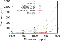
(a)

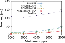
(b)

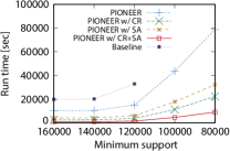
(c)

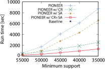
(d)

Figure 2. Impact of minimum support $\theta$ on run time; missing points indicate that a method did not finish within 24 hours; on Pokec, the Baseline did not finish within 24 hours for all minimum support values.

7. Experimental Study

We conduct an experimental study on Pioneer to assess (1) its efficiency, (2) its scalability, and (3) the accuracy of our approximations. We also assess (4) the effectiveness of PARM. We implemented all algorithms in C++ and ran experiments on a Linux server with 512GB of main memory and an Intel(R) Xeon(R) CPU E5-2699v3 processor. Some experimental settings and results (e.g., length $k$ and approximation factors) are in the supplementary file.

7.1. Experimental Setting

Dataset. We use four real-world graphs with edge labels and vertex attributes: knowledge graph Nell (Carlson et al., 2010), coauthorship information network MiCo (Auer et al., 2007), knowledge graph extracted from Wikipedia DBpedia (Auer et al., 2007), and social network service Pokec. We also use two types of synthetic graphs, uniform and exponential. They differ on how we generate edges; in uniform, we generate edges between randomly selected vertices following a uniform distribution, while in exponential we follow an exponential distribution. We vary the number of vertices from 1M to 4M and generate a fivefold number of edges (i.e, 5M to 20M). Table 7 presents statistics on the data.

Table 2. Data statistics.

	$|\mathcal{V}|$	$|\mathcal{E}|$	$|\mathcal{L}|$	$|\mathcal{A}|$	Avg. Attr.
Nell	46,682	231,634	821	266	1.5
MiCo	100,000	1,080,298	106	29	1.0
DBpedia	1,477,796	2,920,168	504	239	2.7
Pokec	1,666,426	34,817,514	9	36,302	1.1
Synthetic	1M – 4M	5M – 20M	500	500	2.0

Compared methods. We assess a baseline and four variants of Pioneer. Baseline is the algorithm of Section 4.2 without any optimization strategy. Pioneer is our algorithm using the strategies of Section 4.3. Pioneer w/ CR using the candidate reduction of Section 5.1, while Pioneer w/ SA uses the stratified sampling of Section 5.2, and Pioneer w/ CR+SA employs both. All algorithms are parallelized by the technique of Section 6. Further, we compare the run time of CSM-A (Prateek et al., 2020), a method that approximately finds the top-$k$ frequent correlated subgraph pairs, to Pioneer, even though the output of CSM-A is different from that of PARM. Notably, other extant graph association rule mining methods (Fan et al., 2015; Fan and Hu, 2017; Wang et al., 2020; Fan et al., 2022a) do not address the PARM problem and do not have open codes.

Parameters. We set minimum support threshold 1 000 on Nell, 4 000 on MiCo, 120 000 on DBpedia, and 45 000 on Pokec, respectively; both the candidate reduction factor $\psi$ and the sampling rate $\rho$ are set to 0.4; we set the maximum path length $k=2$, and use 32 threads. We compute absolute support, relative support, confidence, and lift. We vary these parameters to evaluate their impacts while using the above values as default parameters.

7.2. Efficiency

Varying minimum support $\theta$. Figure 2 plots run time vs. minimum support on each data. The minimum support directly affects the number of rules to be discovered, hence computational cost. As the minimum support falls, the number of candidate path patterns, and hence run time, grows. Our algorithms outperform the baseline in terms of efficiency. In Pokec, the baseline did not finish within 24 hours due to the large number of attributes.

We observe that the enhanced candidate generation, employed in Ours, is effective in reducing candidate path patterns. Further, our approximation methods reducing the number of candidate path patterns and processed vertices by sampling further reduce the computational cost. Our algorithm employing both of these approximation methods consistently achieves the lowest runtime. Regarding the comparison between those two methods, our algorithm with candidate reduction is more effective than that with sampling on Nell, DBpedia, and Pokec, as the number of candidates is often larger than the number of vertices on those data. In MiCo, on the other hand, candidate reduction is not so effective because it does not reduce the candidates with the default $\psi=0.4$.

Comparison to CSM-A. We juxtapose the run time of Pioneer to that of CSM-A. Figure 3 presents our results. On Pokec, Pioneer is much faster than CSM-A, indicating that CSM-A is less scalable in graph size. On DBpedia Pioneer is less efficient, as DBpedia has a large average number of attributes per vertex, yielding a larger search space for Pioneer than for CSM-A (i.e., we reduce the number of attributes per vertex to one for CSM-A).

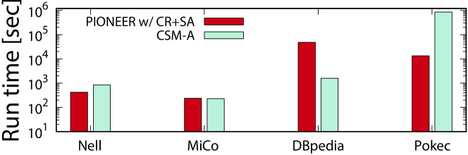
Figure 3. Run time comparison with CSM-A

Varying path length $k$. As the path length $k$ grows, the candidate path patterns increase, thus computation cost grows. On Nell, the number of rules drastically increases as $k$ grows, hence candidate reduction becomes more effective than sampling when $k=3$. With $k=4$, due to the growing number of rules, our algorithms did not finish within 24 hours. Arguably, to effectively find path association rules, we need to either increase the minimum support or reduce approximation factors. On DBpedia the number of path patterns does not grow when $k>2$, so run time does not increase either. This is because some vertices have no outgoing edges, thus most path patterns have length 2. In Pokec, when the $k>2$, the number of reachability patterns increases, thus the run time increases. Overall, our approximation methods work well when $k$ is large, as the run time gap between the exact and approximate algorithms widens.

Varying approximation factors. The approximation factors $\psi$ for candidate reduction and $\rho$ for sampling indicate the degree of approximation. As both decrease, the extent of approximation increases. Notably, when approximation factors are small, run time is low, with the partial exception of Nell. On Nell, the run time of Pioneer w/ SA is high when $\rho=0.2$ due to many false positives that burden the rule discovery step, as Nell is a small graph compared with DBpedia and Pokec. On the other hand, candidate reduction does not increase the number of found frequent path patterns and rules, so the run time of Pioneer w/ CR grows with the approximation factor. In conclusion, sampling effectively reduces run time in large graphs, yet it may not be effective on small graphs.

7.3. Scalability

Table 3. Impact of number of threads on run time [sec]

Dataset	Method	Number of threads
		8	16	32
Nell	Pioneer	754.6	496.2	348.7
	Pioneer w/ CR+SA	74.0	63.2	51.7
MiCo	Pioneer	70.1	37.5	21.0
	Pioneer w/ CR+SA	31.9	17.4	10.0
DBpedia	Pioneer	59 603.0	29 971.0	15 028.0
	Pioneer w/ CR+SA	6 037.0	3 042.0	1 529.0
Pokec	Pioneer	10 039.0	6 197.0	4 038.0
	Pioneer w/ CR+SA	1 981.0	1 103.0	634.0

Varying the number of threads. Table 3 shows the run time vs. the number of threads. As expected, the run time of our algorithms decreases almost linearly as the number of threads rises, especially on larger data.

Table 4. Memory usage [GB]

	Nell	MiCo	DBpedia	Pokec
Pioneer	11.1	0.57	23.9	6.4
Pioneer w/ CR	4.2	0.55	21.5	6.4
Pioneer w/ SA	5.6	0.56	23.8	6.1
Pioneer w/ CR+SA	2.4	0.53	21.5	6.1

Memory usage. Table 4 presents the memory usage of our algorithms. DBpedia raises the highest memory requirements, Pokec the lowest, indicating that memory use depends on the number of candidates more than on graph size. Our algorithms reduce memory usage by reducing candidates, while vertex sampling further reduces memory use by reducing path patterns to be stored for each vertex. When the number of frequent path patterns is large, the approximation methods effectively reduce memory use, as on Nell, confirming our space complexity analysis.

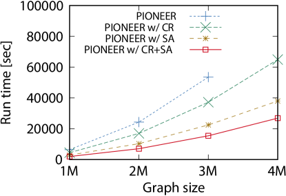
(a)

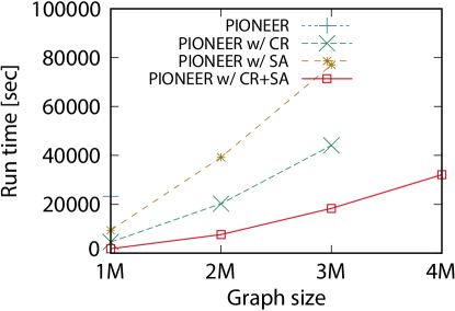
(b)

Figure 4. Scalability to graph size.

Graph size. Figure 4 depicts run time on uniform and exponential synthetic graphs with 0.01 as the relative minimum support. The results suggest that run time grows linearly. Thus, our algorithms are highly scalable to large graphs. On uniform data, vertex sampling is more effective than candidate reduction, while on exponential data, candidate reduction proves to be more effective, since it works best when the maximum degree deviates far from the average.

7.4. Accuracy

We evaluate our approximation methods in comparison to exact ones in terms of recall and precision. Recall is the fraction of true frequent rules that are found and precision is the fraction of found frequent rules that are true; thus, both recall and precision are the value 1.0 if approximation methods return the same results of the exact algorithm. Both recall and precision are quite high in MiCo, DBpedia, and Pokec. In DBpedia, they do not fall even if we set $\psi$ and $\rho$ to 0.2. In Nell, such measures fall as the approximation factors decrease. When applying candidate reduction, the number of matched vertices and the maximum in-degrees are small in Nell, so the missing probabilities become large by Lemma 7. Still, as the difference between the maximum and average in-degrees is large in DBpedia and Pokec, we may reduce candidates without compromising accuracy. Vertex sampling leads to more inaccuracies on Nell and MiCo, which are small compared to DBpedia and Pokec; our approximation methods work well on large graphs.

Table 5. Impact of approximation factors on accuracy.

$\psi$ and $\rho$	CR		SA		CR+SA
	Recall	Precis	Recall	Precis	Recall	Precis
0.2	0.046	1.0	0.9999	0.495	0.046	0.500
0.4	0.233	1.0	0.9999	0.999	0.233	0.998
0.6	0.532	1.0	0.9999	0.9999	0.532	0.9999
0.8	0.797	1.0	0.9999	0.9999	0.797	0.9999

(a) Nell

$\psi$ and $\rho$	CR		SA		CR+SA
	Recall	Precis	Recall	Precis	Recall	Precis
0.2	1.0	1.0	1.0	0.978	1.0	0.978
0.4	1.0	1.0	1.0	0.882	1.0	0.882
0.6	1.0	1.0	1.0	0.938	1.0	0.938
0.8	1.0	1.0	0.978	1.0	0.978	1.0

(b) MiCo

$\psi$ and $\rho$	CR		SA		CR+SA
	Recall	Precis	Recall	Precis	Recall	Precis
0.2	1.0	1.0	1.0	1.0	1.0	1.0
0.4	1.0	1.0	1.0	1.0	1.0	1.0
0.6	1.0	1.0	1.0	1.0	1.0	1.0
0.8	1.0	1.0	1.0	1.0	1.0	1.0

(c) DBpedia

$\psi$ and $\rho$	CR		SA		CR+SA
	Recall	Precis	Recall	Precis	Recall	Precis
0.2	1.0	1.0	0.934	0.983	0.934	0.983
0.4	1.0	1.0	0.967	0.983	0.967	0.983
0.6	1.0	1.0	0.984	0.986	0.984	0.984
0.8	1.0	1.0	0.984	0.984	0.984	0.984

(d) Pokec

7.5. Effectiveness

To our knowledge, no previous work can find path association rules. Besides, PARM does not target quantitatively measurable ground-truth outcomes. We evaluate PARM’s effectiveness qualitatively, by applying it for bias checking and for knowledge extraction.

Bias checking. Detecting data bias is essential for building machine learning models that avoid algorithmic biases. In particular, gender biases in datasets are evaluated in several works (Levy et al., 2021; Imtiaz et al., 2019) We apply PARM to check gender bias in Pokec. We evaluate biases among female and male persons with respect to the education of their friends, comparing the support and confidence of rules of the form $\langle\{\texttt{gender}\}\rangle\Rightarrow\langle\{\},\texttt{follows},\{\texttt{education:A}\}\rangle$. We found 671 rules of the above pattern with $\theta=500$. The sums of absolute supports for males and females are 296 855 and 466 725, respectively, and the sums of confidences are 2.45 and 1.43, respectively. Since the numbers of vertices with male and female are 804 327 and 828 275, i.e., the number of females is larger than that of males, this result suggests that male persons are more likely to have friends who registered their educations than females. In particular, the sum of absolute supports for males who unset their ages is three times larger than that for females who unset their ages (151 240 vs 53 370) Thus, Pokec contains a gender bias in this case. It follows that one should take care when using Pokec to train ML models.

Knowledge extraction. We discuss experimentally found rules.

Nell. We discovered a rule indicating that if a ‘television station’ (vertex $v$) is part of a ‘company’ employing a ‘CEO’, then $v$ is also part of a ‘company’ employing a ‘professor’. Notably, in Nell, there are no vertices associated with both a CEO and a professor, and companies employing both roles are rare. This rule thus elucidates the operations of large organizations.

DBpedia We identified the rule that individuals with a registered birthplace are usually born in populated areas, with confidence of 0.997. This rule thus implies that births in unpopulated places exist. We found three such types: (a) significant buildings like palaces; (b) areas, such as lakes that are now considered unpopulated; and (c) incomplete data, especially in Africa and South America. These findings highlight potential areas for DBpedia’s expansion.

We found 60 places that miss a label of “populatedPlace” among 302 places included in the rules, for example, ”Misiones Province”, ”Al Bahah Province”, and ”Oaxaca”. Other 242 places are significant buildings and areas, and thus we can remove them easily to add the label. PARM helps to explainably complement missing labels.

Pokec. We mined the rule that female users who have not set their ages and are within 2 hops of other female users are likely to follow male users who also have not set their ages, with a confidence of 0.63. However, the confidence of this rule is lower compared to some other rules that have confidence over 0.8. This pattern sheds light on social dynamics in the network. We also observed a rule involving reachability; namely, men in their 20s who are within 4 hops of men who unset their ages are also reachable within 4 hops from women in their 20s, with a confidence of 0.999. This rule illustrates how PARM facilitates connectivity analysis in social networks.

8. Conclusion

We introduced the problem of path association rule mining (PARM), which finds regularities among path patterns in a single large graph, and developed Pioneer, an algorithm for PARM. Our experimental study confirms that Pioneer efficiently finds interesting patterns. In the future, we will extend our method to find top-$k$ rules by novel measures capturing features of path patterns, extend patterns to subgraphs, and add a step that computes other measures.

Appendix A Notations

Table 6 gathers the notations we employ.

Table 6. Notations employed.

Notation	Definition
$\mathcal{A}$, $a$	Set of all attributes, an attribute
$A(v)$	Set of attributes associated with vertex $v$
$p$	Path pattern
$\mathcal{V}(p)$	Set of vertices matching path pattern $p$
$A_{i}$	$i^{\mathrm{th}}$ set of attributes in path pattern
$e_{i}$	$i^{\mathrm{th}}$ edge label in path pattern
$r$ or $p_{x}\Rightarrow p_{y}$	Rule, antecedent $p_{x}$ and consequent $p_{y}$
$\mathcal{P}_{i}$	Set of simple path patterns with $i$ path length
$\mathcal{P}^{*}$	Set of reachability path patterns
$\mathcal{C}$	Set of candidates
$\mathcal{R}$	Set of rules
$\mathcal{L}_{T}$	Set of target edge labels
$\mathcal{A}_{T}$	Set of target attributes
$k$	Maximum path length
$\theta$	Support threshold
$d_{m}$	The largest in-degree among vertices
$\mathcal{E}(A,\ell)$	Set of $\ell$-labeled edges adjacent to $A$-covering vertex
$\mathcal{V}(A,\ell)$	Set of $A$-covering vertices with $\ell$-labeled outgoing edge

Appendix B Related work (Cont’d)

Path queries. Since PARM aims to discover regularities between paths, it relates to path queries on graphs, an active field of study (Angles et al., 2017, 2019; Sasaki et al., 2022; Valstar et al., 2017). However, path queries do not aim to find frequent path patterns. In addition, SPARQL systems can find the number of paths that match given patterns, but it does not focus on frequent mining and measures of data mining such as confidence and lifts, so they do not directely support association rule mining.

Recent real-life query logs for Wikidata (Vrandečić and Krötzsch, 2014) showed that more than 90% of queries are path patterns (Bonifati et al., 2020, 2019). Due to this fact, path patterns are often used in graph analysis instead of subgraph patterns to understand real-world relationships. In that sense, PARM can be useful in real-world analysis.

Appendix C Proof

Theorem 1.

PARM is NP-hard.

Proof sketch: We reduce the NP-hard frequent itemset mining problem (Yang, 2004; Bessiere et al., 2020) to PARM. Given an instance of frequent itemset mining, we build, in polynomial time, a graph without edges, where each node corresponds to a transaction and a set of attributes to a set of items. Solving PARM on this graph amounts to solving the frequent itemset mining problem. Thus, if PARM were solvable in polynomial time, we would solve frequent itemset mining problem in polynomial time too. Hence PARM is NP-hard. $\square$

Theorem 2.

If $p\subset p^{\prime}$, $\mathcal{V}(p)\supseteq\mathcal{V}(p^{\prime})$.

Proof.

If $p^{\prime}$ dominates $p$, then $p$ is no longer than $p^{\prime}$, the edge labels $\ell_{0},\ldots,\ell_{n-1}$ on $p$ and $\ell^{\prime}_{0},\ldots,\ell^{\prime}_{n-1}$ on $p^{\prime}$ are the same in the same order, and the attribute sets in $p$ are subsets of those in $p^{\prime}$, $A_{i}\subseteq A^{\prime}_{i}$ for $i=0\ldots n$. Thus, any vertex that matches $p^{\prime}$ also matches $p$, i.e., $\mathcal{V}(p)\supseteq\mathcal{V}(p^{\prime})$. ∎

Lemma 0.

If the prefix of a path pattern is infrequent, the whole pattern is infrequent.

Proof.

If vertex $v$ matches a whole path pattern $p=\langle A_{0},$ $\ell_{1},\ldots,$ $\ell_{m},A_{m},\ldots,\ell_{n},A_{n}\rangle$, then $v$ also matches the prefix $\langle A_{0},$ $\ell_{1},\ldots,$ $\ell_{m},$ $A_{m}\rangle$ where $m<n$. In reverse, if $v$ does not match the prefix $\langle A_{0},\ell_{1},\ldots,$ $\ell_{m},A_{m}\rangle$, then it does not match the whole pattern $\langle A_{0},\ell_{1},$ $\ldots,$ $\ell_{m},$ $A_{m},\ldots,$ $\ell_{n},A_{n}\rangle$ either. Therefore, if the prefix of a path pattern is infrequent, then the whole path pattern is infrequent. ∎

Lemma 0.

If path pattern $p$ is infrequent and $p^{\prime}$ comprises $A_{i}^{\prime}\supseteq A_{i}$ and $\ell_{i}^{\prime}=\ell_{i}$ for all $i$, then $p^{\prime}$ is also infrequent.

Proof.

If vertex $v$ does not match path pattern $p$, then $v$ does not match $p^{\prime}$ either, as each vertex’s set of attributes in $p^{\prime}$ is a superset of the respective set in $p$. Therefore, if $p$ is infrequent, $p^{\prime}$ is also infrequent. ∎

Lemma 0.

Given length $i>0$, edge label $\ell$, and attribute set $A$, the number of vertices that match a path pattern of length $i$ ending with $\langle\ell,A\rangle$ is upper-bounded by $|\mathcal{E}(A,\ell)|\cdot{d_{m}}^{i-1}$ where $d_{m}$ is the maximum in-degree in the graph.

Proof.

$|\mathcal{E}(A,\ell)|$ is the number of edges with label $\ell$ that connect to a vertex whose attribute set includes $A$. Given path pattern $p=\langle A_{0},\ell,A\rangle$, where $A_{0}$ is an arbitrary attribute set, the maximum number of vertices that may match $p$ is $|\mathcal{E}(A,\ell)|$. This number rises by at most a factor of $d_{m}$ per unit of path length added to its prefix, hence the number of vertices matching a path pattern of length $i$ ending with $\langle\ell,A\rangle$ is upper-bounded by $|\mathcal{E}(A,\ell)|\cdot{d_{m}}^{i-1}$. ∎

Lemma 0.

Given length $i>0$, attribute set $A$, and edge label $\ell$, the number of vertices that match path pattern of the form $p=\langle\ldots,\ell_{i-2},A,\ell,A_{i},\ldots\rangle$ is upper-bounded by $|\mathcal{V}(A,\ell)|\cdot{d_{m}}^{i-1}$ where $d_{m}$ is the maximum in-degree in the graph..

Proof.

$|\mathcal{V}(A,\ell)|$ is the number of vertices whose attribute set covers $A$ and which have an out-going edge with label $\ell$. Given path pattern $p^{\prime}=\langle A,\ell,A_{1}\rangle$, where $A_{0}$ is an arbitrary attribute set, the maximum number of vertices that may match $p^{\prime}$ is $|\mathcal{V}(A,\ell)|$. If $p^{\prime}$ is extended on the suffix to $p^{\prime\prime}=\langle A,\ell,A_{1},\ldots\rangle$, the number of vertices that match $p^{\prime\prime}$ does not increase by Theorem 2. Yet matching vertices grow by at most a factor of $d_{m}$ per unit of length added to the path’s prefix, as in Lemma 5. Hence, the number of vertices matching path pattern $p=\langle\ldots,\ell_{i-2},A,\ell,A_{i},\ldots\rangle$ is upper-bounded by $|\mathcal{V}(A,\ell)|\cdot{d_{m}}^{i-1}$. ∎

Theorem 7.

Given a frequent path pattern $p$ of length $i$ ending with $\langle\ell,A\rangle$, the probability that $p$ is pruned is $P\left(\theta>|\mathcal{V}(p)|\frac{{d_{m}}^{\psi(i-1)}}{c}\right)$, where $c$ is the ratio of $|\mathcal{V}(p)|$ to $|\mathcal{E}(A,\ell)|$, i.e., $|\mathcal{V}(p)|=c|\mathcal{E}(A,\ell)|$.

Proof.

The approximate candidate reduction removes a candidate if $|\mathcal{E}(A,\ell)|{d_{m}}^{\psi(i-1)}<\theta$. Since $|\mathcal{V}(p)|=c|\mathcal{E}(A,\ell)|$, it is:

$$P\left(\theta>|\mathcal{E}(A,\ell)|{{d_{m}}^{\psi(i-1)}}\right)$$

$$= P\left(\theta>|\mathcal{V}(p)|\frac{{d_{m}}^{\psi(i-1)}}{c}\right)$$

∎

Lemma 0.

If $v\in\mathcal{V}$ has no target attributes and no outgoing edges with target labels, then $v$ has no matched path patterns.

Proof.

If $v$ does not match any attributes, it does not become a source of path pattern; similarly, if $v$ has no outgoing-edges in target edges, it has no $\ell_{1}$ in path patterns; the lemma follows. ∎

Appendix D Pseudo-code

input : Graph $\mathcal{G}$, minimum support $\theta$, maximum length $k$

output : set of rules $\mathcal{R}$

1 If minimum support is relative then $\theta\leftarrow\theta|\mathcal{V}|$

2 ${\mathcal{P}}_{0},\ldots,{\mathcal{P}}_{k},{\mathcal{P}}^{*},\mathcal{R}\leftarrow\varnothing$

3 ${\mathcal{C}^{A}}\leftarrow\forall a\in\mathcal{A}$

4 while ${\mathcal{C}}^{A}\neq\varnothing$ do

5       ${\mathcal{P}}_{0}\leftarrow{\mathcal{P}}_{0}\cup$ DiscoverAtt(${\mathcal{C}}^{A},\mathcal{G},\theta$)

6       ${\mathcal{C}}^{A}\leftarrow$ GenerateCandidate($\mathcal{P}_{0}$)

7      

8$(\mathcal{L}_{T},\mathcal{A}_{T})\leftarrow$ MatchedEdges($\mathcal{P}_{0},\mathcal{G}$)

9 for $i=1$ to $k$ do

10       ${\mathcal{C}}^{S}\leftarrow$VerticalExtend(${\mathcal{P}}_{i-1},\mathcal{L}_{T},\mathcal{A}_{T}$)

11       while ${\mathcal{C}}^{S}\neq\varnothing$ do

12             ${\mathcal{P}}_{i}\leftarrow{\mathcal{P}}_{i}\cup$ DiscoverSimple(${\mathcal{C}}^{S},\mathcal{G},\theta$)

13             ${\mathcal{C}}^{S}\leftarrow$ HorizontalExtend(${\mathcal{P}}_{i}$)

14            

15      

16

17$\mathcal{V}_{T}\leftarrow$BFS($\mathcal{L}_{T},\mathcal{G},k$)

18 ${\mathcal{C}}^{*}\leftarrow\forall p$ computed by $\mathcal{L}_{T},\mathcal{A}_{T},\mathcal{P}_{0}$

19 while ${\mathcal{C}}^{*}\neq\varnothing$ do

20       ${\mathcal{P}}^{*}\leftarrow{\mathcal{P}}^{*}\cup$ DiscoverReachable(${\mathcal{C}}^{*},\mathcal{G},\theta,\mathcal{V}_{T}$)

21       ${\mathcal{C}}^{*}\leftarrow$ HorizontalExtend(${\mathcal{P}}^{*}$)

22      

23

24${\mathcal{C}}^{R}\leftarrow\forall(p\Rightarrow p^{\prime})$ such that $p,p^{\prime}$ are unit path patterns $\in\mathcal{P}_{1}\cup\mathcal{P}^{*}$

25 while ${\mathcal{C}}^{R}\neq\varnothing$ do

26       $\mathcal{R}\leftarrow\mathcal{R}\cup$ DiscoverRule(${\mathcal{C}}^{R},\mathcal{G},\theta$)

27       ${\mathcal{C}}^{R}\leftarrow\forall(p\Rightarrow p^{\prime})$ so that either $p$ or $p^{\prime}$ are horizontally and vertically extended path patterns in $\mathcal{R}$.

28      

29ComputeMetrics$(\mathcal{R})$

30 return the set of rules;

Algorithm 1 Pioneer algorithm

Algorithm 1 presents an algorithm of Pioneer in pseudo-code. Each function named Discover* searches for vertices matched with candidates and finds frequent patterns (Lines 5, 11, 16, and 20). Lines 2–7 comprise the step of the frequent attribute set discovery, which follows the same logic as prior work (i.e., the Apriori algorithm (Agrawal et al., 1993)) and also computes edge labels and attributes of targets (Line 7). Lines 8–12 make up the frequent simple path pattern discovery step, which extends already found frequent path patterns vertically and horizontally to form new candidate path patterns. Lines 13–17 show the frequent reachability path pattern discovery step, which conducts a breadth-first search for each frequent edge label from each vertex to obtains a set of reached vertices $\mathcal{V}_{T}$, and then discovers a set of frequent reachability path patterns. Eventually, the rule discovery step in Lines 18–22 first generates candidate rules that are pairs of either simple or reachability unit path patterns of length 1; it mines rules among those candidates and proceeds iteratively by extending the path patterns in the rules it discovers finds both horizontally and vertically. Lastly, it computes measures for all discovered rules.

Appendix E Additional experiments

E.1. Dataset

We use four real-world graphs with edge labels and vertex attributes:

• Nell (Carlson et al., 2010) is a knowledge graph about organizations crawled from the web; it features vertex attributes such as CEO, musician, company, and university, and edge labels such as companyceo, competeswith, and worksat.

• MiCo (Auer et al., 2007) is a coauthorship information network from Microsoft; its attributes and edge labels are embedded in integers.

• DBpedia (Auer et al., 2007) is a knowledge graph extracted from Wikipedia, featuring vertex attributes such as actor, award, person, and place, and edge labels such as child, spouse, and deathPlace. The vertex attribute and edge labels are types of vertices and relationships.

• Pokec is a social network service popular in Slovenia; it features vertex attributes such as age, gender, city, and music, and edge labels such as follows, likes, and locatedIn; we divide edges labeled with follows into seven groups according to out-degree value: single, verysmall, small, average, large, verylarge, and hub are corresponding to 1, 2–4, 5–14, 15–29, 30–49, 50–100, and over 100 out-degrees, respectively.

These datasets are open publicly, so please see their Github in detail. We also use two types of synthetic graphs, uniform and exponential. They differ on how we generate edges; in uniform, we generate edges between randomly selected vertices following a uniform distribution, while in exponential we follow an exponential distribution. We vary the number of vertices from 1M to 4M, while generating a fivefold number of edges (i.e, 5M to 20M). Table 7 presents statistics on the data.

We here note that there are no suitable benchmarks for our problem. For example, a benchmark LDBC (Erling et al., 2015) uses synthetic graphs generated by Graphalytics (Iosup et al., 2020), but they lack vertex attributes and labeled edges. Therefore, we use real-world graphs in various domains and simple synthetic graphs for evaluating scalability.

Table 7. Data statistics.

	$|\mathcal{V}|$	$|\mathcal{E}|$	$|\mathcal{L}|$	$|\mathcal{A}|$	Avg. Attr.
Nell	46,682	231,634	821	266	1.5
MiCo	100,000	1,080,298	106	29	1.0
DBpedia	1,477,796	2,920,168	504	239	2.7
Pokec	1,666,426	34,817,514	9	36,302	1.1
Synthetic	1M – 4M	5M – 20M	500	500	2.0

E.2. Efficiency in detail

Run time analysis. Our results indicate that the data size is not a dominant factor in the run time. For instance, DBpedia takes a longer time in Pokec even though Pokec is larger than DBpedia and the minimum support in Pokec is set smaller than that in DBpedia. To further investigate this matter, we plot, in Figure 5, the distribution of run time components on each step. Table 8 shows the numbers of frequent attribute sets, patterns, and rules on each data set. Table 9 shows the numbers of path pattern types in rules.

We observe that the run time distribution differs across datasets. On Nell, most time is devoted to finding rules and length-2 simple path patterns. On DBpedia, the run time is predominantly spent in finding length-2 simple patterns. On Pokec, time goes to finding all kinds of path patterns rather than rules. These distributions of run time are generally consistent with the numbers of patterns and rules in Table 8; overall, our results corroborate our time complexity analysis, where the numbers of candidates highly affect run time.

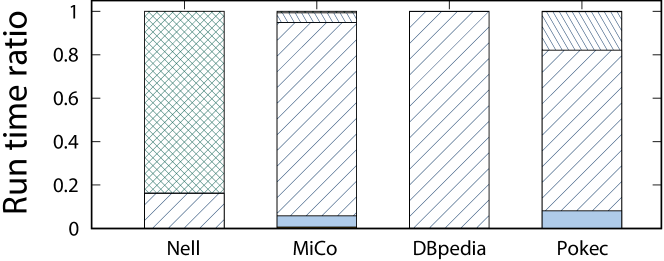
Figure 5. Run time ratio

Table 8. Numbers of path patterns and rules.

	Nell	MiCo	DBpedia	Pokec
Attribute sets	21	7	14	8
Simple paths	2,275	18	6	10
Reachability paths	35	6	6	31
Rules	1,373,707	45	36	61

Table 9. Numbers of pattern types in rules.

	Nell	MiCo	DBpedia	Pokec
1 simple paths	8,828	16	36	20
2 simple paths	2,708,882	55	0	0
Reachability paths	15,704	19	36	102

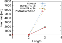
(a)

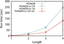
(b)

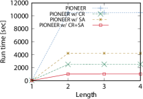
(c)

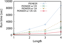
(d)

Figure 6. Impact of length on run time; missing plots indicate that the methods did not finish within 24 hours.

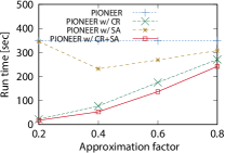
(a)

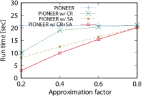
(b)

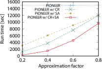
(c)

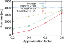
(d)

Figure 7. Impact of approximation factors on run time

Varying path length $k$. As the path length $k$ grows, the candidate path patterns increase, thus computation cost grows. Figure 6 plots run time vs. $k$, setting minimum support $\theta$ to 1 800 in Nell, 140 000 in DBpedia, and 50 000 in Pokec. We do not show the baseline’s run time as it did not finish within 24 hours for $k\geq 3$ on all data. Notably, the run time grows vs. $k$, with the partial exception of DBpedia. On Nell, the number of rules drastically increases as $k$ grows, hence candidate reduction becomes more effective than sampling when $k=3$. With $k=4$, due to the growing number of rules, our algorithms did not finish within 24 hours. Arguably, to effectively find path association rules, we need to either increase the minimum support or reduce approximation factors. On DBpedia the number of path patterns does not grow when $k>2$, so run time does not increase either (see Table 9). This is because some vertices have no outgoing edges, thus most path patterns have length 2. In Pokec, when the $k>2$, the number of reachability patterns increases, thus the run time increases. Overall, our approximation methods work well when $k$ is large, as the run time gap between the exact and approximate algorithms widens.

Varying approximation factors $\psi$ and $\rho$. The approximation factors $\psi$ for candidate reduction and $\rho$ for sampling indicate the degree of approximation. As both decrease, the extent of approximation increases. Figure 7 plots run time varying approximation factor value for both $\psi$ and $\rho$. Notably, when approximation factors are small, run time is low, with the partial exception of Nell. On Nell, the run time of Pioneer w/ SA is high when $\rho=0.2$ due to many false positives that burden the rule discovery step, as Nell is a small graph compared with DBpedia and Pokec. On the other hand, candidate reduction does not increase the number of found frequent path patterns and rules, so the run time of Pioneer w/ CR grows with the approximation factor. In conclusion, sampling effectively reduces run time in large graphs, yet it may not be effective on small graphs.

E.3. CSM-A setting

We juxtapose the run time of our algorithms to that of CSM-A. CSM-A has three parameters minimum support $\theta$, distance threshold $h$, and the size of outputs $k$. We describe how to set each value in each dataset.

First, we set the same number of rules found by our algorithm to $k$ in Table 8. Second, we set zero to $h$; zero is the lightest parameter on CSM-A. As $h$ increases, the search space increases. Finally, we set $\theta$ to values that CSM-A found at least $k$ patterns. CSM-A works on labeled graphs rather than attributed graphs, so we use one of the attributes in each vertex as a vertex label. Since CSM-A processes only labeled graphs, we reduce the number of vertex attributes in Nell, DBpedia, and Pokec to 1 for CSM-A, letting our algorithms work on a larger search space than CSM-A. MiCo is a labeled graph, so we let our algorithms and CSM-A operate on the same graph. As CSM-A runs on a single thread, we also run our algorithms single-threaded in this comparison. We summarize the parameters in Table 10.

Table 10. The parameters in CSM-A.

Parameter	Nell	MiCo	DBpedia	Pokec
Output size $k$	1,373,707	46	35	61
Distance threshold $h$	0	0	0	0
Minimum support $\theta$	30	7,000	10,000	80,000

We here report the run time and the number of patterns to show that we appropriately set $\theta$ in CSM-A. Table 11 shows the performance of CSM-A in each dataset and two values of minimum supports. One minimum support can output $k$ rules and another minimum support outputs a smaller number of rules than $k$. We can see the minimum support and the number of found rules are different across methods. For example, in Nell, our method that we set the minimum support as 1,000 found 1,373,514 rules while CSM-A needs to set the minimum support as 30 for finding 1,373,514 rules.

Table 11. The impact of minimum support $\theta$ in CSM-A.

Dataset	$\theta$	Run time [sec]	# patterns
Nell	30	835.9	1,373,514
	40	296.7	355,467
Mico	7,000	228.1	45
	8,000	194.6	21
DBpedia	10,000	1 593.2	35
	20,000	821.5	1
Pokec	80,000	848 899	61
	90,000	687 949	28

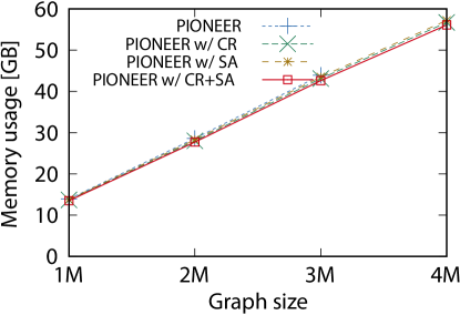
(a)

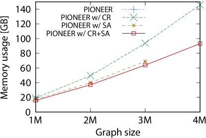
(b)

Figure 8. Memory usage to graph size.

E.4. Memory usage on synthetic graphs

Figure 8 shows the memory usage on synthetic graphs. This results show the our approximation can reduce the memory usage; In particular, sampling can reduce the memory usage compared to the candidate reduction in the exponential, though the candidate reduction can accelerate run time. This is because for large scale graphs, the sampling can significantly reduce the number of vertices to store as the source of paths.

References

- (1)
- Agrawal et al. (1993) Rakesh Agrawal, Tomasz Imieliński, and Arun Swami. 1993. Mining association rules between sets of items in large databases. In SIGMOD. 207–216.
- Agrawal and Srikant (1995) Rakesh Agrawal and Ramakrishnan Srikant. 1995. Mining sequential patterns. In Proceedings of the eleventh international conference on data engineering. 3–14.
- Alipourlangouri and Chiang (2022) Morteza Alipourlangouri and Fei Chiang. 2022. Discovery of Keys for Graphs. In DaWaK. 202–208.
- Angles et al. (2017) Renzo Angles, Marcelo Arenas, Pablo Barceló, Aidan Hogan, Juan L. Reutter, and Domagoj Vrgoc. 2017. Foundations of modern query languages for graph databases. ACM Comput. Surv. 50, 5 (2017), 68:1–68:40.
- Angles et al. (2019) Renzo Angles, Juan L. Reutter, and Hannes Voigt. 2019. Graph query languages. In Encyclopedia of Big Data Technologies.
- Auer et al. (2007) Sören Auer, Christian Bizer, Georgi Kobilarov, Jens Lehmann, Richard Cyganiak, and Zachary Ives. 2007. Dbpedia: A nucleus for a web of open data. In The semantic web. 722–735.
- Bessiere et al. (2020) Christian Bessiere, Mohamed-Bachir Belaid, and Nadjib Lazaar. 2020. Computational Complexity of Three Central Problems in Itemset Mining. arXiv preprint arXiv:2012.02619 (2020).
- Bonifati et al. (2019) Angela Bonifati, Wim Martens, and Thomas Timm. 2019. Navigating the Maze of Wikidata Query Logs. In WWW. 127–138.
- Bonifati et al. (2020) Angela Bonifati, Wim Martens, and Thomas Timm. 2020. An analytical study of large SPARQL query logs. The VLDB Journal (2020), 655–679.
- Bringmann and Nijssen (2008) Björn Bringmann and Siegfried Nijssen. 2008. What is frequent in a single graph?. In PAKDD. 858–863.
- Calders et al. (2008) Toon Calders, Jan Ramon, and Dries Van Dyck. 2008. Anti-monotonic overlap-graph support measures. In ICDM. 73–82.
- Carlson et al. (2010) Andrew Carlson, Justin Betteridge, Bryan Kisiel, Burr Settles, Estevam R Hruschka, and Tom M Mitchell. 2010. Toward an architecture for never-ending language learning. In AAAI. 1306–1313.
- Chen et al. (2022) Lihan Chen, Sihang Jiang, Jingping Liu, Chao Wang, Sheng Zhang, Chenhao Xie, Jiaqing Liang, Yanghua Xiao, and Rui Song. 2022. Rule mining over knowledge graphs via reinforcement learning. Knowledge-Based Systems 242 (2022), 108371.
- Chen et al. (2016) Yang Chen, Daisy Zhe Wang, and Sean Goldberg. 2016. ScaLeKB: scalable learning and inference over large knowledge bases. The VLDB Journal 25, 6 (2016), 893–918.
- Dastin (2018) Jeffrey Dastin. 2018. Rpt-insight-amazon scraps secret ai recruiting tool that showed bias against women. Reuters (2018).
- De Bie (2013) Tijl De Bie. 2013. Subjective interestingness in exploratory data mining. In International Symposium on Intelligent Data Analysis. 19–31.
- Deng et al. (2021) Junning Deng, Bo Kang, Jefrey Lijffijt, and Tijl De Bie. 2021. Mining explainable local and global subgraph patterns with surprising densities. Data Mining and Knowledge Discovery 35, 1 (2021), 321–371.
- Elseidy et al. (2014) Mohammed Elseidy, Ehab Abdelhamid, Spiros Skiadopoulos, and Panos Kalnis. 2014. Grami: Frequent subgraph and pattern mining in a single large graph. PVLDB 7, 7 (2014), 517–528.
- Erling et al. (2015) Orri Erling, Alex Averbuch, Josep Larriba-Pey, Hassan Chafi, Andrey Gubichev, Arnau Prat, Minh-Duc Pham, and Peter Boncz. 2015. The LDBC social network benchmark: Interactive workload. In SIGMOD. 619–630.
- Fan et al. (2020a) Grace Fan, Wenfei Fan, Yuanhao Li, Ping Lu, Chao Tian, and Jingren Zhou. 2020a. Extending Graph Patterns with Conditions. In SIGMOD. 715–729.
- Fan et al. (2022a) Wenfei Fan, Wenzhi Fu, Ruochun Jin, Ping Lu, and Chao Tian. 2022a. Discovering association rules from big graphs. PVLDB 15, 7 (2022), 1479–1492.
- Fan et al. (2022b) Wenfei Fan, Ziyan Han, Yaoshu Wang, and Min Xie. 2022b. Parallel Rule Discovery from Large Datasets by Sampling. In SIGMOD. 384–398.
- Fan and Hu (2017) Wenfei Fan and Chunming Hu. 2017. Big graph analyses: From queries to dependencies and association rules. Data Science and Engineering 2, 1 (2017), 36–55.
- Fan et al. (2020b) Wenfei Fan, Chunming Hu, Xueli Liu, and Ping Lu. 2020b. Discovering graph functional dependencies. TODS 45, 3 (2020), 1–42.
- Fan et al. (2015) Wenfei Fan, Xin Wang, Yinghui Wu, and Jingbo Xu. 2015. Association rules with graph patterns. PVLDB 8, 12 (2015), 1502–1513.
- Fan et al. (2016) Wenfei Fan, Yinghui Wu, and Jingbo Xu. 2016. Adding counting quantifiers to graph patterns. In SIGMOD. 1215–1230.
- Fariha et al. (2013) Anna Fariha, Chowdhury Farhan Ahmed, Carson Kai-Sang Leung, SM Abdullah, and Longbing Cao. 2013. Mining frequent patterns from human interactions in meetings using directed acyclic graphs. In PAKDD. 38–49.
- Fisher et al. (2019) Joseph Fisher, Dave Palfrey, Christos Christodoulopoulos, and Arpit Mittal. 2019. Measuring social bias in knowledge graph embeddings. arXiv preprint arXiv:1912.02761 (2019).
- Fournier-Viger et al. (2014) Philippe Fournier-Viger, Ted Gueniche, Souleymane Zida, and Vincent S Tseng. 2014. ERMiner: sequential rule mining using equivalence classes. In International Symposium on Intelligent Data Analysis. 108–119.
- Fournier-Viger et al. (2015) Philippe Fournier-Viger, Cheng-Wei Wu, Vincent S Tseng, Longbing Cao, and Roger Nkambou. 2015. Mining partially-ordered sequential rules common to multiple sequences. TKDE 27, 8 (2015), 2203–2216.
- Galárraga et al. (2013) Luis Antonio Galárraga, Christina Teflioudi, Katja Hose, and Fabian Suchanek. 2013. AMIE: association rule mining under incomplete evidence in ontological knowledge bases. In WWW. 413–422.
- Haller and Hadler (2006) Max Haller and Markus Hadler. 2006. How social relations and structures can produce happiness and unhappiness: An international comparative analysis. Social indicators research 75, 2 (2006), 169–216.
- Han et al. (2019) Myoungji Han, Hyunjoon Kim, Geonmo Gu, Kunsoo Park, and Wook-Shin Han. 2019. Efficient subgraph matching: Harmonizing dynamic programming, adaptive matching order, and failing set together. In SIGMOD. 1429–1446.
- House et al. (1988) James S House, Karl R Landis, and Debra Umberson. 1988. Social relationships and health. Science 241, 4865 (1988), 540–545.
- Huynh et al. (2022) Bao Huynh, Lam BQ Nguyen, Duc HM Nguyen, Ngoc Thanh Nguyen, Hung-Son Nguyen, Tuyn Pham, Tri Pham, Loan TT Nguyen, Trinh DD Nguyen, and Bay Vo. 2022. Mining Association Rules from a Single Large Graph. Cybernetics and Systems (2022), 1–15.
- Imtiaz et al. (2019) Nasif Imtiaz, Justin Middleton, Joymallya Chakraborty, Neill Robson, Gina Bai, and Emerson Murphy-Hill. 2019. Investigating the effects of gender bias on GitHub. In ICSE. 700–711.
- Inokuchi et al. ([n.d.]) Akihiro Inokuchi, Takashi Washio, and Hiroshi Motoda. [n.d.]. An apriori-based algorithm for mining frequent substructures from graph data. In PKDD. 13–23.
- Iosup et al. (2020) Alexandru Iosup, Ahmed Musaafir, Alexandru Uta, Arnau Prat Pérez, Gábor Szárnyas, Hassan Chafi, Ilie Gabriel Tănase, Lifeng Nai, Michael Anderson, Mihai Capotă, et al. 2020. The LDBC Graphalytics Benchmark. arXiv preprint arXiv:2011.15028 (2020).
- Kaur and Kang (2016) Manpreet Kaur and Shivani Kang. 2016. Market Basket Analysis: Identify the changing trends of market data using association rule mining. Procedia computer science 85 (2016), 78–85.
- Ke et al. (2009) Yiping Ke, James Cheng, and Jeffrey Xu Yu. 2009. Efficient discovery of frequent correlated subgraph pairs. In ICDM. 239–248.
- Lee et al. (2001) C-H Lee, Y-H Kim, and P-K Rhee. 2001. Web personalization expert with combining collaborative filtering and association rule mining technique. Expert Systems with Applications 21, 3 (2001), 131–137.
- Lee et al. (2012) Jinsoo Lee, Wook-Shin Han, Romans Kasperovics, and Jeong-Hoon Lee. 2012. An in-depth comparison of subgraph isomorphism algorithms in graph databases. PVLDB 6, 2 (2012), 133–144.
- Lee et al. (1998) Sau Dan Lee, David W Cheung, and Ben Kao. 1998. Is sampling useful in data mining? a case in the maintenance of discovered association rules. Data Mining and Knowledge Discovery 2, 3 (1998), 233–262.
- Levy et al. (2021) Shahar Levy, Koren Lazar, and Gabriel Stanovsky. 2021. Collecting a Large-Scale Gender Bias Dataset for Coreference Resolution and Machine Translation. In EMNLP. 2470–2480.
- Mallik et al. (2014) Saurav Mallik, Anirban Mukhopadhyay, and Ujjwal Maulik. 2014. RANWAR: rank-based weighted association rule mining from gene expression and methylation data. IEEE transactions on nanobioscience 14, 1 (2014), 59–66.
- Manola et al. (2004) Frank Manola, Eric Miller, Brian McBride, et al. 2004. RDF primer. W3C recommendation 10, 1-107 (2004), 6.
- Meilicke et al. (2020) Christian Meilicke, Melisachew Wudage Chekol, Manuel Fink, and Heiner Stuckenschmidt. 2020. Reinforced anytime bottom up rule learning for knowledge graph completion. arXiv preprint arXiv:2004.04412 (2020).
- Meng and Tu (2017) Jinghan Meng and Yi-cheng Tu. 2017. Flexible and feasible support measures for mining frequent patterns in large labeled graphs. In SIGMOD. 391–402.
- Namaki et al. (2017) Mohammad Hossein Namaki, Yinghui Wu, Qi Song, Peng Lin, and Tingjian Ge. 2017. Discovering graph temporal association rules. In CIKM. 1697–1706.
- Nikolakaki et al. (2018) Sofia Maria Nikolakaki, Charalampos Mavroforakis, Alina Ene, and Evimaria Terzi. 2018. Mining tours and paths in activity networks. In WWW. 459–468.
- Nowozin et al. (2007) Sebastian Nowozin, Gokhan Bakir, and Koji Tsuda. 2007. Discriminative subsequence mining for action classification. In ICCV. 1–8.
- Ortona et al. (2018) Stefano Ortona, Venkata Vamsikrishna Meduri, and Paolo Papotti. 2018. Robust discovery of positive and negative rules in knowledge bases. In ICDE. 1168–1179.
- Pellegrina et al. (2019) Leonardo Pellegrina, Matteo Riondato, and Fabio Vandin. 2019. Hypothesis testing and statistically-sound pattern mining. In KDD. 3215–3216.
- Prateek et al. (2020) Arneish Prateek, Arijit Khan, Akshit Goyal, and Sayan Ranu. 2020. Mining top-k pairs of correlated subgraphs in a large network. PVLDB 13, 9 (2020), 1511–1524.
- Samiullah et al. (2014) Md Samiullah, Chowdhury Farhan Ahmed, Anna Fariha, Md Rafiqul Islam, and Nicolas Lachiche. 2014. Mining frequent correlated graphs with a new measure. Expert systems with applications 41, 4 (2014), 1847–1863.
- Sasaki et al. (2022) Yuya Sasaki, George Fletcher, and Onizuka Makoto. 2022. Language-aware Indexing for Conjunctive Path Queries. In ICDE. 661–673.
- Schmitz et al. (2006) Christoph Schmitz, Andreas Hotho, Robert Jäschke, and Gerd Stumme. 2006. Mining association rules in folksonomies. In Data science and classification. 261–270.
- Shelokar et al. (2014) Prakash Shelokar, Arnaud Quirin, and Óscar Cordón. 2014. Three-objective subgraph mining using multiobjective evolutionary programming. J. Comput. System Sci. 80, 1 (2014), 16–26.
- Thompson (2002) S Thompson. 2002. Sampling. Wiley.
- Toivonen et al. (1996) Hannu Toivonen et al. 1996. Sampling large databases for association rules. In VLDB, Vol. 96. 134–145.
- Valstar et al. (2017) Lucien D.J. Valstar, George H.L. Fletcher, and Yuichi Yoshida. 2017. Landmark Indexing for Evaluation of Label-Constrained Reachability Queries. In SIGMOD. 345–358.
- Vanetik et al. (2002) Natalia Vanetik, Ehud Gudes, and Solomon Eyal Shimony. 2002. Computing frequent graph patterns from semistructured data. In ICDM. 458–465.
- Vrandečić and Krötzsch (2014) Denny Vrandečić and Markus Krötzsch. 2014. Wikidata: a free collaborative knowledgebase. Commun. ACM 57, 10 (2014), 78–85.
- Wang et al. (2020) Xin Wang, Yang Xu, and Huayi Zhan. 2020. Extending association rules with graph patterns. Expert Systems with Applications 141 (2020), 112897.
- Weikum (2021) Gerhard Weikum. 2021. Knowledge Graphs 2021: A Data Odyssey. PVLDB 14, 12 (2021), 3233–3238.
- Yan and Han (2002) Xifeng Yan and Jiawei Han. 2002. gspan: Graph-based substructure pattern mining. In ICDM. 721–724.
- Yang (2004) Guizhen Yang. 2004. The complexity of mining maximal frequent itemsets and maximal frequent patterns. In KDD. 344–353.
- Zaki et al. (1998) Mohammed Javeed Zaki, Neal Lesh, and Mitsunori Ogihara. 1998. PlanMine: Sequence Mining for Plan Failures.. In KDD. 369–373.
- Zhao and Bhowmick (2003) Qiankun Zhao and Sourav S Bhowmick. 2003. Association rule mining: A survey. Nanyang Technological University 135 (2003).