Blockchain-Enabled Dynamic Spectrum Sharing for Satellite and Terrestrial Communication Networks

Abstract

Dynamic spectrum sharing (DSS) between satellite and terrestrial networks has increasingly engaged the academic and industrial sectors. Nevertheless, facilitating secure, efficient and scalable sharing continues to pose a pivotal challenge. Emerging as a promising technology to bridge the trust gap among multiple participants, blockchain has been envisioned to enable DSS in a decentralized manner. However, satellites with limited resources may struggle to support the frequent interactions required by blockchain networks. Additionally, given the extensive coverage of satellites, spectrum sharing needs vary by regions, challenging traditional blockchain approaches to accommodate differences. In this work, a partitioned, self-governed, and customized dynamic spectrum sharing approach (PSC-DSS) is proposed for spectrum sharing between satellite access networks and terrestrial access networks. This approach establishes a sharded and tiered architecture which allows various regions to manage spectrum autonomously while jointly maintaining a single blockchain ledger. Moreover, a spectrum-consensus integrated mechanism, which decouples DSS process and couples it with blockchain consensus protocol, is designed to enable regions to conduct DSS transactions in parallel and dynamically innovate spectrum sharing schemes without affecting others. Furthermore, a theoretical framework is derived to justify the stability performance of PSC-DSS. Finally, simulations and experiments are conducted to validate the advantageous performance of PSC-DSS in terms of low-overhead, high efficiency, and robust stability.

I Introduction

Satellite access networks (SANs) are envisioned to be broadly supplement to terrestrial access networks (TANs) to realize global seamless coverage, operating in frequency bands below 6 GHz for providing mobile satellite services [1, 2]. With the increasing of wireless devices and the expansion of satellite constellations, there is a marked escalation in the demand for spectrum resources. However, the spectrum resources at below 6 GHz band have been almost exhaustively licensed while the Federal Communications Commission (FCC) reports that less than 85% of this band is actually used [3]. High demand and low utilization of spectrum motivate the development of spectrum sharing technologies that reallocate temporarily idle resources between SANs and TANs.

The typical spectrum sharing solutions include static spectrum sharing and dynamic spectrum sharing (DSS) [4]. Static spectrum sharing experiences low utilization efficiency due to its fixed and exclusive manner. Thus, DSS is progressively becoming the mainstream to further exploit the potential of limited spectrum resources supply [5]. Several DSS solutions have been developed, such as the well-known spectrum access system (SAS) for citizens broadband radio service (CBRS) system [6]. However, existing DSS solutions faces major challenges in terms of security and scalability.

For security, all spectrum users must place absolute trust in the spectrum administrators, such as SAS administrators for CBRS [7], which are presumed to be trustworthy to perform reasonable spectrum allocation decisions using a centralized database-based system. This mandatory trust, however, inevitably leads the risk of single point failure and raises security concerns over the malicious exploitation of critical nodes, especially in the evolving threat landscape of SANs. For scalability, centralized DSS models impose excessive regulatory pressure on regulators as an increasing number of heterogeneous participants from regions or countries become involved in SANs, consequently leading to limited scalability. Therefore, a new DSS paradigm that is secure and scalable is in high demand.

As an emerging technology, blockchain has shown the potential to improve the security of DSS due to its ability to enable trusted transaction processing and immutable ledger keeping among mutually distrustful participants, even if a certain portion of them behave maliciously [7, 8]. The support for the self-executing smart contracts also empowers blockchain to improve the scalability of DSS by distributing responsibility and workload among various participants in a decentralized manner. Many government agencies and organizations have voiced consider blockchain as a possible paradigm to enable DSS in the future, such as FCC [9], China Communications Standards Association [10], and l’Agence Nationale des Fréquences [11]. Meanwhile, several concrete solutions [12, 13] and innovative studies have been proposed [6, 14, 7]. However, employing blockchain for DSS in SANs still faces the following important challenges:

• High overhead: Conventional blockchain-based DSS architecture requires that each transaction be validated by all blockchain nodes. Moreover, additional cross-chain infrastructure is needed to enable interoperability and communication between different chains. This architecture is impractical for DSS in SANs, given the limited resources available on satellites.

• Limited efficiency: The prevailing blockchain-based DSS process currently involves distributing each step sequentially to distinct blocks, meaning that a round of consensus only performs one step of the DSS. However, this process is time-consuming and power-intensive, which falls significantly short in meeting the crucial needs for both efficient and large-scale spectrum sharing.

• Constrained flexibility: Existing blockchain-based DSS solutions require all participants adhere to a unified spectrum sharing scheme, constraining flexibility in the evolving SANs that face a growing diversity of participants with dynamic and varied requirements. For practical purposes, an optimal solution should support for both forward and backward compatibility, especially for SANs undergoing rapid evolution.

Moreover, the characterization of the stability of blockchain systems in SANs is of importance because of ultra-expensive costs for deploying satellites and installing blockchain in satellites. An accurate theoretical framework is essential to thoroughly understand how such systems operate, which kinds of system factors can affect their performance, what the principles that these system factors influence the performance, and further obtain insights on network design guidance [15]. Different from wired networks, the features of SANs, including unstable channel, severe interference, untrusted physical entities, etc., pose many extra difficulties in both theoretical analysis and practical implementations. Therefore, faced with such a complex environment, it is crucial but challenging to consider these features in analyzing the stability of blockchain systems in SANs. However, the study that considers these features simultaneously when applying blockchain to DSS in SANs, is yet inadequate.

The above observations inspire us to develop a partitioned, self-governed and customized DSS approach dubbed PSC-DSS, aiming to provide a low-overhead, highly efficient and flexible DSS solution for SANs. This approach leverages the principle of blockchain to bridge the gap among various parties and establish healthy relationships among diverse spectrum sharing participants in SANs. In order to advance the understanding of the proposed PSC-DSS, we address three fundamental questions in this paper, as follows.

• How to construct the PSC-DSS for SANs: To tackle this question, we establish a two-tier multi-region blockchain-based DSS architecture with a single-chain structure, where the spectrum autonomy within each region and global information synchronization achieved through upper-level interaction. Importantly, this architecture allows different region s to adopt various spectrum sharing schemes and enables interaction across region s without the need for any additional cross-chain infrastructure.

• How to perform the PSC-DSS in SANs: To address this question, we design a spectrum-consensus integrated mechanism, which couples blockchain consensus protocol with spectrum sharing scheme. This mechanism redesigns the consensus protocol and restructures the DSS procedure, enabling regions to parallelly process DSS transactions and dynamically innovate spectrum sharing schemes without affecting others. Furthermore, the generalized workflow and main functions are introduced to advance the understanding of the proposed mechanism.

• How to analyze the performance of the PSC-DSS within SANs: Faced with this question, we first build a theoretical framework to study the probability of system stability. Based on the derived closed-form expression, we further explore the influence of the unstable wireless environment of satellite-terrestrial communication on system stability using stochastic geometry.

Furthermore, simulation and experiment results demonstrate the performance of this work in terms of low-overhead, high efficiency, and robust stability under various network parameters. Pivotal insights and design guidelines are provided for further implementations and extensions.

The rest of this work is organized as follows. Section II introduces the overview of PSC-DSS including architecture, entities, and workflow. Section III presents the proposed spectrum-consensus integrated mechanism, detailing the main functions and procedures. Section IV analyses the stability performance. Simulations and experiments are conducted in Section V. Section VI reviews the existing related works. Finally, Section VII concludes this work.

II PSC-DSS Overview

In this section, the architecture of PSC-DSS is first introduced. Then, participants and main tasks are defined. Finally, the work flow of PSC-DSS is described.

II-A Two-tier Multi-region Architecture

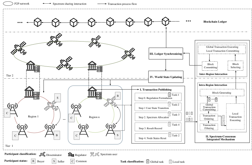
Figure 1: PSC-DSS architecture

As illustrated in Fig. 1, the proposed PSC-DSS is composed of two tiers and multiple regions. It is worth noting that all participants in PSC-DSS only maintain a single-chain, which is highly different with existing sharding-based DSS solutions.

Tier 1 consists of multiple specific regions, each including a regulator node, base stations, and satellites. Each region autonomously manages its spectrum, encompassing the selection and dynamic evolution of suitable spectrum sharing schemes. Transactions related to a specific region are packaged into a block and submitted to tier 2 after the intra-region interaction of the proposed spectrum-consensus integrated mechanism is performed. Accordingly, spectrum sharing can be undertaken separately and parallelly, and thus enabling efficient and large-scale spectrum sharing in SANs. Furthermore, following this sharding-based design, spectrum management rights are devolved to regions, and promoting more activity and flexible spectral business.

Tier 2, curated by all regulator nodes and many satellites, is responsible for receiving and disseminating the blocks submitted by tier 1, then performing the inter-region interaction of the proposed spectrum-consensus integrated mechanism. After that, all regulator nodes update their world state and blockchain ledger, which are then synchronized with base stations and satellites in tier 1. Therefore, all participants record only one ledger, which reduces resource consumption caused by maintaining multi-region blockchain networks, especially for the resource-constrained satellites. This single-chain design enables any DSS transaction in any region can be traced back through the blockchain, thus realizing simple but trustworthy cross-region supervision and enhancing the recognition of on-chain DSS transactions.

Moreover, PSC-DSS demonstrates robust backward and forward compatibility, allowing for integration with existing distributed spectrum sharing systems. An example of PSC-DSS instantiation is seen in CBRS, where the concept of a “region” aligns with a CBRS “zone” and the “tier” concept corresponds to the relationship between the FCC and CBDS. Furthermore, PSC-DSS supports the dynamic evolution of spectrum sharing schemes for each region by updating a key function in the proposed spectrum-consensus integrated mechanism (as detailed in Section III), without impacting others.

II-B Participants

PSC-DSS involves 3 types of participants: regulators, spectrum users, and disseminators. These participants each play a critical role in spectrum sharing system and blockchain system, respectively.

Regulators are spectrum management entities that publish regulations on spectrum sharing in their jurisdiction, and provide regulation-compliant spectrum allocation service to spectrum users in their regions. For example, regulators can be distributed FCC entities to make regulations for spectrum sharing in U.S., or they can be SAS servers that implement specific spectrum sharing schemes in certain regions. In blockchain networks, regulators are responsible for starting a round of intra-region interaction, and submitting the generated block to satellites in tier 2. Besides, regulators are also in charge of performing the inter-region interaction in tier 2.

Spectrum users include base stations and satellites in tier 1 for spectrum access assignment. Additionally, this category can be expanded to encompass other entities such as access points, road side units, and campus hotspots. A spectrum user are categorized into 3 status: buyer, and seller, common. Buyer status indicates that a spectrum user needs additional spectrum to meet specific demands, while seller status represents one who has surplus spectrum available for sublease. Common status is assigned to the spectrum users with stable demand who neither need to buy nor sell spectrum. In blockchain network, spectrum users are responsible for performing intra-region interactions as directed by the regulator in their region.

Disseminators are consisted of satellites that have no spectrum spectrum access assignment needs in their regions, considering potential security risks from interest entanglements. They are in charge of receiving blocks submitted by regulators and propagating these blocks into all participants in tier 2. A bootstrapper is opened in a selected disseminator to order the blocks and bootstrap regulators for a new round of inter-region interaction.

Disseminators do not participate in spectrum sharing and consensus in blockchain. Therefore, among all participants in the PSC-DSS, only regulators and spectrum users are defined as blockchain participants. They engage in transaction verification, task execution, and ledger updates.

II-C Main Tasks

In PSC-DSS, spectrum sharing-related tasks are typically classified into 4 types, where Task-1 is a global task that needs coordinated implementation in tier 2, while Tasks 2 to 4 are local tasks that can be executed within a specific region. Each type of task can be derived into many independent blockchain transactions, and a blockchain transaction can contain multiple types of tasks.

Task-1 Regulation formulation: PSC-DSS allows regulators to issue rules on various tasks, such as identifying spectrum regions, specifying interference models, and updating participant’s information. It is the action guideline for spectrum sharing schemes, and all subsequent spectrum sharing-related tasks are performed on this basis.

Task-2 User status transition: Spectrum users specify their spectrum needs, including frequency band, current status and target status for this frequency band, price, duration of use, and other relevant details. Regulators publish this task to reset the status of spectrum users after completing a round of spectrum allocation process.

Task-3 Spectrum allocation: PSC-DSS performs spectrum sharing based on user requests, including parameters for predefined spectrum sharing scheme, user information contained in Task-2, and other required details. Various customize spectrum sharing schemes are allowed to lunched in difference regions to suit their actual situation.

Task-4 Result record: Irreversible spectrum requests, allocation results, and current spectrum status are recorded. This task provides a complete track of the spectrum sharing process for all frequency band. Thus, efficient supervisions and audits can be implemented based on this task.

To reduce the overhead of base stations and satellites, PSC-DSS stipulates that only Task-2 is issued by spectrum users during their spectrum application stage, while all other tasks are issued by regulators.

II-D Main Workflow

Since the PSC-DSS architecture is envisioned to be broadly inter-operative and to support multiple advanced wireless services and standards, this work focuses on the most basic spectrum sharing approach for which the procedure is shown in Fig. 1.

In step 0, the preparation for spectrum sharing, regulators should issue transactions for Task-1 to publish regulations on spectrum usage and management. This step may be performed periodically or irregularly, depending on updates to spectrum sharing regulations, changes in current spectrum sharing requirements, and evaluations for spectrum sharing implementation plans.

In step 1, spectrum users initiate status requests to regulators to publish transactions for Task-2, according to their own needs. For example, if a user has idle spectrum available for sublease, its status in the corresponding frequency band is changed from common to seller. Details about the current information of users and parameters for subsequent spectrum allocation in step 3 are submitted to the system.

In step 2, transactions for Task-3 are published by regulators to trigger the specific spectrum sharing schemes. An explicit spectrum allocation solution is obtained for all frequency bands on sale, encompassing spectrum access decisions, operational parameters, business settings, etc.

In step 3, regulators publish transactions for Task-4 to record the whole spectrum sharing process. For a specific frequency band, transfer details such as involved users and price, and operational parameters like transmission power, will be comprehensively recorded. For a spectrum user, specifics in request, transitions in status, changes in assets are captured.

In step 4, the status of users are reset as common through the transactions pertain to Task-2 published by regulators. This step marks the end of this round of spectrum sharing. If a user has a persistent requirement to maintain a certain status, it needs to re-initiate Task-2 as a new transaction in step1, considering the rapid changes in terms of network topology, channel usage, and participants in SANs.

Each of the above steps is accomplished by executing a blockchain transaction. Therefore, from the perspective of blockchain, the process that each step undergoes is described as follows. Step I is for transaction publishing. All transactions for tasks are published by regulators with the aim of reducing the operational overhead of base stations and satellites. Although Task-2 is issued by users to actively transition their status, users merely send task requests to regulators. After a fixed period of time or once a certain number of requests have been collected, regulators generate transactions for these requests. Step II is to perform the proposed spectrum-consensus integrated mechanism. During this step, transactions are packaged into blocks and executed by blockchain participants. Specifically, transactions related to global tasks are executed by regulators, while transactions for local tasks are executed by blockchain participants within corresponding regions, with only the results of these executions being recorded in blocks. In step III, each blcokchain participant updates its local ledger copy to match the latest blockchain state on the network. Accordingly, in step IV, the world state is first updated in all regulators and then propagated to base stations and satellites within each region. Details pertaining to all tasks are recorded and updated to ensure the accuracy and currency of spectrum management in the PSC-DSS.

III Spectrum-Consensus Integrated Mechanism

In this section, the proposed spectrum-consensus integrated mechanism based on the PSC-DSS architecture are detailed. First, the main components for this mechanism are introduced. Then, key functions and corresponding procedures are described.

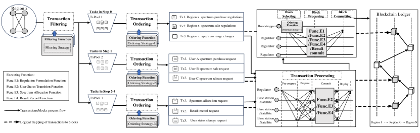
Figure 2: The process of spectrum-consensus integrated mechanism

III-A Main Components

The proposed mechanism shown in Fig. 2, comprises intra-region and inter-region interactions, which couple spectrum sharing scheme with blockchain consensus protocol. Details of each component are described as follows.

III-A1 Intra-region Interaction

The process of intra-region interaction consists of 3 steps: transaction filtering, transaction ordering, and transaction processing. Through these steps, transactions for local tasks are executed and packaged into blocks.

Transaction filtering: As the execution modes and participants of tasks vary across the steps 1-4, regulators employ Filtering Function to filter transactions corresponding to tasks into 3 distinct transaction pools (TxPools). TxPool1 stores transactions for Task-1 in step 0, TxPool2 manages transactions for Task-2 in step 1, and TxPool 3 is responsible for transactions related to Tasks 2 to 4 across steps 2 to 4. Furthermore, transactions from Tasks 2 to 4 which aims to apply for a cross-region spectrum sharing, are also put into TxPool1. This filtering facilitates asynchronous transaction processing and parallel resource allocation.

Transaction Ordering: According to Section III-D, the sequence of executing spectrum sharing tasks critically influences the sharing process. Additionally, the priority of task execution varies and develops across different regions. Consequently, regulators utilize Ordering Functions to sequence the transactions taken from TxPools, determining which transactions are packaged into a block and their order. It is worth noting that the transactions in TxPool3 and the cross-region spectrum sharing transactions in TxPool1 involved three types tasks (i.e., Tasks 2-4), which are processed sequentially. Therefore, theses transactions should be ordered following a fixed rule and be packaged into one block. Other transactions can correspond to a different ordering strategies, allowing for adaptive and logical management at each step of the spectrum sharing process.

Transaction Processing: Each blockchain participant invokes Executing Functions to execute transactions sequentially. These functions are specifically identified as Func.E2, Func.E3, and Func.E4, detailed in Section III-B. Notably, transactions in TxPool1 involve global tasks and requires the participation from all regulators, so there is no corresponding executing function Func.E1 in this step. Instead, transactions in TxPool1 are packaged directly into blocks after consensus verification and submitted to tier 2 for execution. To be specific, a regulator packages the ordered transactions into a block and broadcasts it to blockchain participants within its region. For the block containing transactions from TxPool1, the practical byzantine fault tolerance (PBFT) consensus protocol is initiated. For the block with transactions from TxPools2 or TxPools3, during the commit stage of PBFT consensus protocol, blockchain participants trigger the corresponding executing functions (e.g., Func.E2 for TxPool2, Func.E3, Func.E4, Func.E2 sequentially for TxPool3). Then, the processed results replace the original transactions in the block to form a new block. Subsequently, commit message for this new block is generated and broadcast to all blockchain participants. Once the regulator receives commit messages from more than $\frac{2}{3}$ blockchain participants in its region, it confirms the validity of the new block. Upon validation, the block is then broadcast to disseminators, marking the completion of intra-region interactions and triggering the start of the next round.

Algorithm 1 Ordering Function

1:TxPool1, TxPool2, TxPool3, BlPool

2:Transaction Lists $TxLists$, candidate block $CadiBl$

3:if $TxPool1$ is not empty then

4:     Order $Tx$ following FCFS model

5:     Append them into $TxLists(1)$

6:end if

7:if $TxPool2$ is not empty then

8:     Order $Tx$ following FCFS model

9:     Append them into $TxLists(2)$

10:end if

11:if $TxPool3$ is not empty then

12:     Order SpecAllo_Intra type $Tx$ into $AlloTxlist$;

13:     for each $Tx$ in $AlloTxlist$ do

14:         Order the corresponding ResRecord and StatusRest type sequentially after the $Tx$

15:         Append $AlloTxlist$ into $TxLists(3)$

16:     end for

17:end if

18:if $BlPool$ is not empty then

19:     Order blocks following FCFS model

20:     Append them into $CandiBlList$

21:end if

22:Return $TxLists$, $CandiBl\leftarrow CandiBlList(1)$

III-A2 Intra-region Interaction

After receiving blocks from regulators, disseminators transmit these blocks to all disseminators and regulators through inter-satellite links (ISL). Then, the following steps are performed sequentially.

Block Selecting: The bootstrapper activated in a selected disseminator triggers the Ordering Function to propose a candidate block, and transmit it to all regulators.

Block Processing: If the candidate block contains transactions from TxPool1, regulators invoke Executing Function (i.e., Func. E1-Func. E4). Then, the execution results replace the regional transactions in the candidate block. Conversely, if the candidate block contains execution results from transactions in TxPool2 or TxPools3, regulators verify these results.

Block Committing: After receiving feedback from $\frac{1}{2}$ regulators, the bootstrapper sends a confirmation message to indicate that the candidate block has been authenticated by the whole network. Then, the blockchain ledger and the world state are updated, marking the completion of inter-region interactions and triggering the start of the next round.

Algorithm 2 Func.E1 for processing Task-1

1:Candidate block $CandiBl$

2:Processed candidate block $ProCandiBl$

3:for each transaction $Tx$ with $Global$ type in $CandiBl$ do

4:     Trigger $SC.GloFunc$ to process the $Tx$

5:     The process result replaces the original $Tx$ in $CandiBl$;

6:end for

7:return $ProCandiBl\leftarrow CandiBl$

III-B Key Functions

As shown in Fig. 2, the proposed mechanism involves 3 types of key functions, which enable specialized transaction execution. Importantly, these functions can vary across different regions and can be dynamically updated without impacting other regions. In this work, algorithms corresponding to these key functions are presented as use cases to advance the understanding of PSC-DSS.

III-B1 Filtering Function

This function filters transactions to corresponding TxPools according to their types. Based on Section II-C, Global tasks for global operations are placed into TxPool1. StatusTrans tasks for user status transitions are allocated to TxPool2. SpecAllo, ResRecord, and StatusReset tasks, which are for spectrum allocation, result recording, and status resetting respectively, are assigned to TxPool3.

III-B2 Ordering Function

This function sequences transactions taken from TxPools, and decides how the boostrapper selects the next candidate block from multiple blocks transmitted by regulators. As presented in Alg. 1, this work adopts first-come-first-serve (FCFS) model to order transactions in TxPool1 and TxPool2, appending them to $TxLists(1)$ and $TxLists(2)$. Similarly, a candidate block $CandiBl$ is selected from the bootstrapper’s block pool $BlPool$. Especially, for transactions in TxPool3, transactions with SpecAllo type are first ordered following the FCFS model. Then, for each SpecAllo transaction, the corresponding ResRecord and StatusReset transactions follow sequentially and are appended into $TxLists(3)$. Finally, a transaction list $TxLists$ including ordered transactions for TxPools is generated. Each element of $TxLists$ (e.g. $TxLists(1)$) will be packaged into one block to be processed.

Algorithm 3 Func.E2 for processing Task-2

1:$TxLists$, $RecResultTx$, $AlloResultTx$

2:Region block $RegBl$, shareable spectrum list $SharedSpecList$, terminal list $AwaitTerList$

3:if $TxLists(2)$ is not empty then

4:     for each $Tx$ do

5:         if $Tx$ is for $seller$ status then

6:              Add seller’s spectrum to $SharedSpecList$;

7:         else if $Tx$ is for $buyer$ status then

8:              Add buyer’s terminal to $AwaitTerList$;

9:         end if

10:         Invoke $SC.StaFunc$, obtain processed result ${Tx}^{{}^{\prime}}$

11:         Add ${Tx}^{{}^{\prime}}$ into $RegBl$

12:     end for

13:     return $RegBl$, $SharedSpecList$, $AwaitTerList$

14:end if

15:if $TxLists(3)$ is not empty then

16:     Collect all $Tx$ with $StatusReset$ type

17:     invoke $SC.StaFunc$ to get ${Tx}^{{}^{\prime}}$

18:     Add $AlloResultTx$, $RecResultTx$, ${Tx}^{{}^{\prime}}$ into $RegBl$

19:     return $RegBl$

20:end if

Algorithm 4 Func.E3 for processing Task-3

1:$TxLists$, $SharedSpecList$, $AwaitTerList$

2:$AlloResultTx$, $SpecRecList$

3:if $TxLists(3)$ is not empty then

4:     Add $Tx$ with $SpecAllo$ type into $AlloTxList$

5:     Perform SpecSche($AlloTxList$, $SharedSpecList$, $AwaitTerList$)

6:     Obtain $SpecAlloSolution$ and $SpecRecList$

7:     Invoke $SC.AlloFunc$ to get the result $AlloResultTx$

8:end if

9:return $AlloResultTx$, $SpecRecList$

Algorithm 5 Func.E4 for processing Task-4

1:$TxLists$, $SpecRecList$

2:$RecResultTx$

3:if $TxLists(3)$ is not empty then

4:     Add $ResRecord$ type $Tx$ into $ResRecordTxList$

5:     Add $SpecRecList$ into $ResRecordTxList$ and match each $Tx$

6:     Invoke $SC.RecFunc$ to process $ResRecordTxList$, obtain result $RecResultTx$

7:end if

8:return $RecResultTx$

III-B3 Executing Function

There are 4 functions for transaction execution. Func. E1-Func. E4 are used to execute the Tasks 1 to 4, respectively. Here, a smart contract which includes 4 sub-function (i.e., $GloFunc$, $StaFunc$, $AlloFunc$, $RecFunc$) is used to perform the information change for Tasks 1 to 4.

In Func.E1 (shown in Alg.2), the sub-function $SC.GloFunc$ in smart contract is triggered to process transactions $Tx$ with $Global$ type in $CandiBl$. Then the process results will be added to $CandiBl$ to replace the original transactions to form a new processed candidate block.

In Func.E2 (shown in Alg.3), transactions in $TxList(2)$ are processed by the sub-function in the smart contract ($SC.StaFunc$) to change the status of users included in each $Tx$. The processed results, ${Tx}^{{}^{\prime}}$, are then added to the region block $RegBl$. Additional information, including the details of idle spectrum available for sharing and the information about terminals that require spectrum, are recorded by seller nodes in $SharedSpecList$ and by buyer nodes in $AwaitTerList$, respectively. This information is used to facilitate the execution of the spectrum sharing scheme. For transactions in $TxLists(3)$, all $StatusReset$ type transactions are collected and processed by $SC.StaFunc$ to get a result ${Tx}^{{}^{\prime}}$. Then, the transaction $AlloResultTx$ returned by Func.E3, $RecResultTx$ returned by Func.E4, and the ${Tx}^{{}^{\prime}}$ are sequentially added to $RegBl$. Here, $AlloResultTx$ contains the spectrum allocation results, and $RecResultTx$ details the entire spectrum sharing process.

In Func.E3 (shown in Alg. 4), all $SpecAllo$ type transactions in $Txlists(3)$ are first added to the list $AlloTxList$. Then, a spectrum sharing scheme $SpecSche$ is performed based on $AlloTxList$, $SharedSpecList$, and $AwaitTerList$, obtaining an optimal spectrum sharing solution $SpecAlloSolution$. According to $SpecAlloSolution$, the sub-function $SC.AlloFunc$ in the smart contract is invoked to update the spectrum information to get the result $AlloResultTx$. Besides, details of the entire spectrum sharing process, including requests, parameters for $SpecSche$, and the current spectrum situation, are recorded in $SpecRecList$.

In Func. E4 (shown in Alg.5),, all $ResRecord$ type transactions in $Txlists(3)$ are collected into a list $ResRecordTxList$. Then, $SpecRecList$ is appended to $ResRecordTxList$ by matching its elements. Then, $SC.RecFunc$ is used to process $ResRecordTxList$ and get a result $RecResultTx$.

IV Performance Analysis

In this section, the stability performance of PSC-DSS is analyzed in the perspective of the success rate of reaching consensus, $P_{S}$. Network model and the definition of the success rate of reaching consensus are first introduced. Then, the closed form of $P_{S}$ is derived.

IV-A Network Model

Consider a satellite-terrestrial communication system with $M$ regions, each one contains $N_{s}$ satellites and $N_{g}$ ground nodes (including a regulator’s entity and base stations). We assume that the satellites are located on the surface of the sphere with radius $R_{S}$ according to a homogeneous spherical Poisson point process (SPPP) $\Phi_{S}$ with density $\lambda_{s}$. The locations of ground nodes are further assumed to be distributed on the surface of the Earth with radius $R_{E}$ according to a homogeneous SPPP $\Phi_{G}$ with density $\lambda_{g}$. For the downlink communication shown in Fig. 3(a), the visible spherical cap of a ground node $G_{DL,0}$ with minimum elevation angle $\theta_{\min}$ is expressed as ${\cal A}_{DL,vis}$. The distance between $G_{DL,0}$ and its nearest satellite $S_{DL,0}$ is denoted as $D_{DL,0}$. The distance between $G_{DL,0}$ and the $i$th interference satellite (i.e., ${S_{DL,i}}\in{\Phi_{S}}\cap{{\cal A}_{DL,vis}}\backslash{S_{DL,0}}$) is denoted as $D_{DL,i}$. For the uplink communication shown in Fig. 3(b), the visible spherical cap of a satellite $S_{UL,0}$ with maximum Earth-centered zenith angle $\varphi_{\max}$ is expressed as ${\cal A}_{UL,vis}$. The distance between $S_{UL,0}$ and its nearest ground node $G_{UL,0}$ is denoted as $D_{UL,0}$, and the distance between $S_{UL,0}$ and the $j$th interference ground node (i.e., ${S_{UL,j}}\in{\Phi_{S}}\cap{{\cal A}_{UL,vis}}\backslash{S_{UL,0}}$) is denoted as $D_{UL,j}$.

For the channel model, the Shadowed-Rician fading model is used for the channels between satellites and ground nodes [16]. Following with [17, 18, 19], a gamma random variable is used to approximate the PDF of channel gain ${{{\left|{{h}}\right|}^{2}}}$, which is expressed as

$${f_{{{\left|{{h}}\right|}^{2}}}}\left(x\right)=\frac{1}{{{\beta^{\alpha}}\Gamma\left(\alpha\right)}}{x^{\alpha-1}}\exp\left({-\frac{x}{\beta}}\right),$$ (1)

where $\Gamma(.)$ is the gamma function, $\alpha=\frac{{m{{\left({2{b_{0}}\Omega}\right)}^{2}}}}{{4mb_{0}^{2}+4mb_{0}^{2}\Omega+{\Omega^{2}}}}$ and $\beta=\frac{{2{b_{0}}+\Omega}}{\alpha}$ is the shape and scale parameters, respectively. $m$, $2b_{0}$, and $\Omega$ denote the Nakagami fading coefficient, the average power of scattered component, and the average power of line-of sight component, respectively.

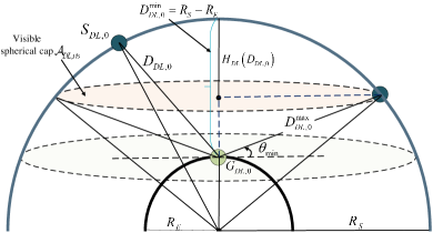
(a) Downlink satellite-terrestrial networks

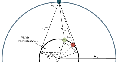
(b) Uplink satellite-terrestrial networks

Figure 3: Illustration of the geometry of downlink and uplink satellite-terrestrial networks

Hence, the revived signal-to-interference-plus-noise ratio (SINR) at $G_{DL,0}$ for the dowlink, can be expressed as

$$\gamma_{DL,0}={\frac{{P_{t}^{S}g_{DL,0}{{\left|{{h_{DL,0}}}\right|}^{2}}D_{DL,0}^{-2}}}{{\sigma_{G}^{2}+\sum\limits_{i\in{\Phi_{S}^{{}^{\prime}}}}{P_{t}^{S}{{\left|{{h_{DL,i}}}\right|}^{2}}g_{DL,i}D_{DL,i}^{-2}}}}},$$ (2)

where $\Phi_{S}^{{}^{\prime}}={\Phi_{S}}\cap{{\cal A}_{DL,vis}}\backslash{\cal A}_{DL,vis}^{{}^{\prime}}\left({{D_{DL,0}}}\right)$ and ${\cal A}{{}^{{}^{\prime}}_{DL,vis}}\left(D_{DL,0}\right)$ denotes the visible spherical cap with the maximization distance $D_{DL,0}$ between $G_{DL,0}$ and satellites, $P_{t}^{S}$ is the transmit power at satellites, $\sigma_{G}^{2}$ is the variance of the AWGN at $G_{DL,0}$, ${{\left|{{h_{DL,x}}}\right|}^{2}}$ denotes the channel gain between $G_{DL,0}$ and $S_{DL,x}$ $\left(x\in\left\{0,i\right\}\right)$, and $g_{DL,x}$ is the effective antenna gain [20] for the signal path from $S_{DL,x}$ to $G_{DL,0}$. Here, $g_{UL,0}=g_{t}^{S}g_{r}^{G}\left(\frac{c}{4\pi f_{c}}\right)^{2}$ and $g_{UL,i}=\bar{g}_{DL}g_{DL,0}$, where $g_{t}^{S}$ is the transmit antenna gain of satellites, $g_{r}^{G}$ is the receive antenna gain of ground nodes, $c$ is the speed of light, and $f_{c}$ is the carrier frequency, $\bar{g}_{DL}\in\left[0,1\right]$ is the interference mitigation factor for downlink [21].

Similarly, the SINR at $S_{UL,0}$ for the uplink, can be expressed as

$$\gamma_{UL,0}={\frac{{P_{t}^{G}g_{UL,0}{{\left|{{h_{UL,0}}}\right|}^{2}}D_{UL,0}^{-2}}}{{\sigma_{S}^{2}+\sum\limits_{j\in{\Phi_{G}^{{}^{\prime}}}}{P_{t}^{G}{{\left|{{h_{UL,j}}}\right|}^{2}}g_{UL,j}D_{UL,i}^{-2}}}}},$$ (3)

where $\Phi_{G}^{{}^{\prime}}={\Phi_{G}}\cap{{\cal A}_{UL,vis}}\backslash{\cal A}_{UL,vis}^{{}^{\prime}}\left({{D_{UL,0}}}\right)$ and ${\cal A}{{}^{{}^{\prime}}_{UL,vis}}\left(D_{UL,0}\right)$ denotes the visible spherical cap with the maximization distance $D_{UL,0}$ between $S_{DL,0}$ and ground nodes, $P_{t}^{G}$ is the transmit power at ground nodes, $\sigma_{G}^{2}$ is the variance of the AWGN at $S_{UL,0}$, ${{\left|{{h_{UL,y}}}\right|}^{2}}$ denotes the channel gain between $S_{UL,0}$ and $G_{UL,y}$ $\left(y\in\left\{0,j\right\}\right)$, $g_{UL,y}$ is the effective antenna gain [20] for the signal path from $G_{UL,y}$ to $S_{UL,0}$. Besides, $g_{UL,0}=g_{t}^{G}g_{r}^{S}\left(\frac{c}{4\pi f_{c}}\right)^{2}$ and $g_{UL,j}=\bar{g}_{UL}g_{UL,0}$, where $g_{t}^{G}$ is the transmit antenna gain of ground nodes, $g_{r}^{S}$ is the receive antenna gain of satellites, and $\bar{g}_{UL}\in\left[0,1\right]$ is the interference mitigation factor for uplink [21].

IV-B Performance Metric

To quantitatively measure the stability performance of PSC-DSS in SANs, the introduction of a specific performance metric is indispensable. Considering the complex environment of SANs, such as unstable channel and sever interference, satellites and ground nodes are inevitably faced with faulty probabilities, denoted as $P_{f}^{S}$ and $P_{f}^{G}$, respectively, which significantly affect the consensus reaching process in intra-region interaction and the inter-region interaction.

Hence, the success rate of reaching consensus in both intra-region interaction and the inter-region interaction, $P_{S}$, is defined as the stability performance metric for PSC-DSS in SANs. In PSC-DSS, the intra-region interaction tolerates no more than $\left\lfloor{\frac{N_{s}+N_{g}}{3}}\right\rfloor$ faulty nodes (including satellites and ground nodes) based on PBFT consensus protocol, and the inter-regin interaction requires no more than $\left\lfloor{\frac{M}{2}}\right\rfloor$ faulty regulators to commit a block. In such case, $P_{S}$ is given as

$$P_{S} =\sum\limits_{i=0}^{\left\lfloor{\frac{{{N_{g}}+{N_{s}}}}{3}}\right\rfloor}{\left[{\left({\sum\limits_{n=0}^{\min(i,{N_{g}}-{\rm{1}})}{\left({1-P_{f}^{G}}\right){P_{n0}}}}\right)\left({\sum\limits_{j=0}^{\left\lfloor{\frac{M}{2}}\right\rfloor}{{P_{j}}}}\right)}\right]}$$

$$+\sum\limits_{i=1}^{\left\lfloor{\frac{{{N_{g}}+{N_{s}}}}{3}}\right\rfloor}{\left[{\left({\sum\limits_{n=1}^{\min(i,{N_{g}})}{P_{f}^{G}{P_{n1}}}}\right)\left({\sum\limits_{j=0}^{\left\lfloor{\frac{M}{2}}\right\rfloor-1}{{P_{j}}}}\right)}\right]},$$ (4)

with

$${P_{n0}} =C_{{N_{g}}-{\rm{1}}}^{n}{\left({P_{f}^{G}}\right)^{n}}{\left({1-P_{f}^{G}}\right)^{{N_{g}}-1-n}}\times{\textbf{1}_{\left\{{i-n<{N_{s}}}\right\}}}$$

$$\;\;\;\;\times C_{{N_{s}}}^{i-n}{\left({P_{f}^{S}}\right)^{i-n}}{\left({1-P_{f}^{S}}\right)^{{N_{s}}-\left({i-n}\right)}},$$ (5)

$${P_{n{\rm{1}}}} =C_{{N_{g}}-{\rm{1}}}^{n-{\rm{1}}}{\left({P_{f}^{G}}\right)^{n-{\rm{1}}}}{\left({1-P_{f}^{G}}\right)^{{N_{g}}-n}}\times{\textbf{1}_{\left\{{i-n<{N_{s}}}\right\}}}$$

$$\;\;\;\;\times C_{{N_{s}}}^{i-n}{\left({P_{f}^{S}}\right)^{i-n}}{\left({1-P_{f}^{S}}\right)^{{N_{s}}-\left({i-n}\right)}},$$ (6)

and

$${P_{j}}={C_{M-1}^{j}{{\left({P_{f}^{G}}\right)}^{j}}{{\left({1-P_{f}^{G}}\right)}^{M-1-j}}},$$ (7)

where ${\textbf{1}_{\left\{.\right\}}}$ is the indicator function, and $C_{a}^{b}$ is the binomial coefficient. Details are given in Appendix A. Fig. 4 shows that the analytical results for $P_{S}$ closely match the simulation results, verifying the correctness of the analysis in (IV-B). We can see that the success rate $P_{S}$ decreases with $P_{f}^{G}$ and $P_{f}^{S}$. Given the conditions $M=60$, $N_{g}=40$, and $N_{s}=20$, PSC-DSS can a faulty probability of over 0.7 for satellites when $P_{f}^{G}=0.03$ and over 0.3 for satellites when $P_{f}^{G}=0.2$.

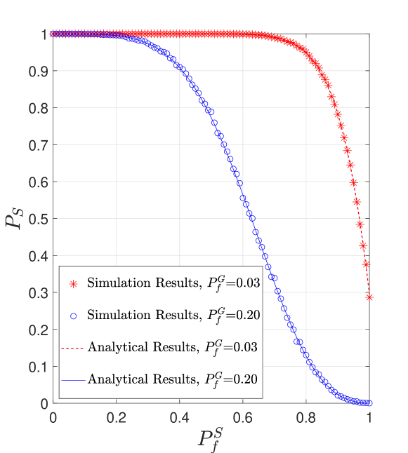
Figure 4: Success rate $P_{S}$ versus faulty probability of satellites $P_{f}^{G}$

However, $P_{f}^{G}$ and $P_{f}^{S}$ are influenced by various factors, such as security outage and transmission outage probabilities. Satellite and base station as communication infrastructure, its security performance is highly valued by countries and regions. Therefore, this work mainly measures the faulty probability of nodes from the perspective of transmission outage. For satellites, a fault occurs when they cannot receive signals from ground nodes through ISLs and satellite-terrestrial communication links. For ground nodes, a fault occurs when they fail to receive signals through wired and satellite-terrestrial communication links. Therefore, $P_{f}^{G}$ and $P_{f}^{S}$ can be expressed as ${P_{f}^{G}}=P_{out}^{DL}\times P_{out}^{WL}$ and ${P_{f}^{S}}=P_{out}^{UL}\times P_{out}^{ISL}$, respectively. Here, $P_{out}^{DL}$ and $P_{out}^{WL}$ are the transmission outage probabilities at ground nodes through the downlink satellite-terrestrial and wired communication links, while $P_{out}^{UL}$ and $P_{out}^{ISL}$ are the outage probabilities at satellites via the uplink satellite-terrestrial link and ISLs. Next, $P_{out}^{DL}$ and $P_{out}^{UL}$ are analyzed in SANs.

IV-C Outage Analysis

The outage probability is characterized when there is at least one transmitter in visible spherical cap, i.e., ${\Phi_{S}({{\cal A}_{DL,vis}})>0}$ and ${\Phi_{G}({{\cal A}_{UL,vis}})>0}$. Thus, $P_{out}^{DL}$ and $P_{out}^{UL}$, are expressed as

$$P_{out}^{DL}\left(\gamma\right) =\Pr\left({\gamma_{DL,0}<\gamma\left|{{\Phi_{S}}\left({{{\cal A}_{DL,vis}}}\right)>0}\right.}\right)$$

$${\rm{}}\times\Pr\left({{\Phi_{S}}\left({{{\cal A}_{DL,vis}}}\right)>0}\right).$$ (8)

and

$$P_{out}^{UL}\left(\gamma\right) =\Pr\left({\gamma_{UL,0}<\gamma\left|{{\Phi_{G}}\left({{{\cal A}_{UL,vis}}}\right)>0}\right.}\right)$$

$${\rm{}}\times\Pr\left({{\Phi_{G}}\left({{{\cal A}_{UL,vis}}}\right)>0}\right),$$ (9)

Following (IV-C) and (IV-C), and based on (2) and (3), there are three fundamental distributions (i.e., the probability of transmitter-visibility, the conditional nearest transmitter distance distribution, and the conditional Laplace transform of the aggregated interfere) for providing the general expressions for $P_{out}^{DL}$ and $P_{out}^{UL}$. Thus, three lemmas are introduced for these fundamental distributions as follows.

Lemma 1 (The Probability of Transmitter-Visibility): The probability that there is at least one satellite in visible spherical cap of a ground node, and the probability that there is at least one ground node in visible spherical cap of a satellite, are respectively given as

$$\Pr\left({\Phi_{S}\left({{{\cal A}_{DL,vis}}}\right)>0}\right)=1-\exp\left(-\lambda_{s}\left|{{{\cal A}_{DL,vis}}}\right|\right)$$

$$=1-\exp\left({-\pi{\lambda_{s}}{R_{S}}\frac{{{{\left({D_{DL,0}^{\max}}\right)}^{\rm{2}}}+2{R_{E}}{R_{S}}-R_{E}^{2}-R_{S}^{2}}}{{{R_{E}}}}}\right),$$ (10)

and

$$\Pr\left({\Phi_{G}\left({{{\cal A}_{UL,vis}}}\right)>0}\right)=1-\exp\left(-\lambda_{g}\left|{{{\cal A}_{UL,vis}}}\right|\right)$$

$$={1-\exp\left({-2\pi{\lambda_{g}}R_{E}^{2}\left({1-\cos{\psi_{\max}}}\right)}\right)},$$ (11)

where $\left|{{{\cal A}}}\right|$ denotes the area of a visible spherical ${{{\cal A}}}$, and ${D_{DL,0}^{\max}}=\sqrt{{{\left({R_{E}\sin{\theta_{\min}}}\right)}^{2}}+R_{S}^{2}-R_{E}^{2}}-R_{E}\sin{\theta_{\min}}$ is the maximum distance between $G_{DL,0}$ and satellites in the downlink communicates.

Proof: See Appendix B.

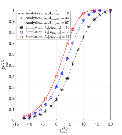
(a) $P_{out}^{DL}$ versus $\gamma_{out}^{DL}$

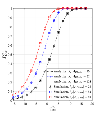
(b) $P_{out}^{UL}$ versus $\gamma_{out}^{UL}$

Figure 5: Outage analysis for fixed $R_{S}-R_{E}=500$ Km, and other parameters are same with Section V-A.

$${\cal G}(s,\lambda,R_{1},R_{2},d_{max},d,\bar{g}) =\exp\left({-\pi{\lambda}\frac{{{R_{1}}}}{{{R_{2}}}}\left({{{d_{\max}^{2}}}-d^{2}}\right)}+{\pi{\lambda}\frac{{{R_{1}}}}{{{R_{2}}}}\frac{{{{d_{\max}^{2\left({\alpha+1}\right)}}}}}{{{\left({s{{\bar{g}}}\beta}\right)}^{\alpha}(\alpha+1)}}{\times{{{}_{2}}{F_{1}}\left({\alpha,\alpha+1;2+\alpha;-\frac{{{d_{\max}^{2}}}}{{s\bar{g}\beta}}}\right)}}}\right)$$ (16)

$$\div\exp\left({\pi{\lambda}\frac{{{R_{1}}}}{{{R_{2}}}}\frac{{d^{2\left({\alpha+1}\right)}}}{{{\left({s{{\bar{g}}}\beta}\right)}^{\alpha}(\alpha+1)}}{\times{{{}_{2}}{F_{1}}\left({\alpha,\alpha+1;2+\alpha;-\frac{{{d^{2}}}}{{s\bar{g}\beta}}}\right)}}}\right)$$

$$\eta\left({\gamma,\delta,{d_{\max}},{d_{\min}},g,\kappa,\lambda,}\right)=\int_{{d_{\min}}}^{{d_{\max}}}{\exp\left({-{\beta^{-1}}\gamma\delta d^{2}}\right)\times\upsilon\left({\gamma,d,d_{\max},\delta,g}\right)}\times\zeta\left({d,{d_{\max}},\kappa,\lambda}\right){\rm{d}}d$$ (19)

$$\zeta\left({d,{d_{\max}},\kappa,\lambda}\right)=\frac{{2d\pi\lambda\kappa\times\exp\left({-\pi\lambda\kappa\left({{d^{2}}+2{R_{E}}{R_{S}}-R_{E}^{2}-R_{S}^{2}}\right)}\right)}}{{1-\exp\left({-\pi\lambda\kappa\left({d_{\max}^{2}+2{R_{E}}{R_{S}}-R_{E}^{2}-R_{S}^{2}}\right)}\right)}}$$ (20)

$$\upsilon\left({\gamma,d,d_{max},\delta,g}\right)=\sum\limits_{m=0}^{\alpha-1}{\left[{\frac{1}{{m!}}\times\sum\limits_{k=0}^{m}{C_{m}^{k}\delta^{2\left({m-k}\right)}{{\left({{\beta^{-1}}\gamma d^{2}}\right)}^{m}}\times{{\left({-1}\right)}^{k}}\frac{{{{\rm{d}}^{k}}\chi\left({\kappa,\lambda,d,{d_{\max}},g}\right)}}{{{\rm{d}}{{\left({{\beta^{-1}}\gamma d^{2}}\right)}^{k}}}}}}\right]}$$ (21)

$$\begin{array}[]{c}\chi\left({\kappa,\lambda,d,{d_{\max}},g}\right)=\exp\left({\pi\lambda\kappa\left({d_{\max}^{2}-d^{2}+\frac{{{{\left({d^{2}g\gamma}\right)}^{-\alpha}}}}{{\alpha+1}}d_{\max}^{2\left({\alpha+1}\right)}{\times_{2}}{F_{1}}\left({\alpha,\alpha+1;2+\alpha;-\frac{{d_{\max}^{2}}}{{d^{2}g\gamma}}}\right)}\right)}\right)\\ \times\exp{\left({\pi{\lambda}\kappa\frac{{{{\left({g\gamma}\right)}^{-\alpha}}}}{{\alpha+1}}d^{2}{\times_{2}}{F_{1}}\left({\alpha,\alpha+1;2+\alpha;-{{\left({g\gamma}\right)}^{-1}}}\right)}\right)^{-1}}\end{array}$$ (24)

Lemma 2 (The Conditional Nearest Transmitter Distance Distribution): Let $D_{DL,0}$ denotes the distance from $G_{DL,0}$ and its nearest transmission satellite $S_{DL,0}$ in ${{{\cal A}_{DL,vis}}}$, and $D_{UL,0}$ denotes the distance from $S_{UL,0}$ and its nearest transmission ground node $G_{UL,0}$ in ${{{\cal A}_{UL,vis}}}$. Then, the probability density functions (PDF) of $D_{DL,0}$ and $D_{UL,0}$, are expressed as

$${f_{{D_{DL,0}}}}\left({{d_{DL,0}}}\right)={\xi_{DL}}{d_{DL,0}}\exp\left({-\pi{\lambda_{s}}\frac{{{R_{S}}}}{{{R_{E}}}}d_{DL,0}^{2}}\right),$$ (12)

and

$${f_{{D_{UL,0}}}}\left({{d_{UL,0}}}\right)={{\xi_{UL}}{d_{UL,0}}\exp\left({-\pi{\lambda_{g}}\frac{{{R_{E}}}}{{{R_{S}}}}d_{UL,0}^{2}}\right)},$$ (13)

respectively, where $d_{DL,0}\in\left[{{D_{DL,0}^{min}},{D_{DL,0}^{max}}}\right]$, $d_{UL,0}\in\left[{{D_{UL,0}^{min}},{D_{UL,0}^{max}}}\right]$, with ${D_{DL,0}^{min}}={D_{UL,0}^{min}}={R_{S}}-{R_{E}}$, ${D_{UL,0}^{max}}=\sqrt{R_{E}^{2}+R_{S}^{2}-2{R_{S}}{R_{E}}\cos{\varphi_{\max}}}$, ${\xi_{DL}}=\frac{{\frac{{2\pi{\lambda_{s}}{R_{s}}}}{{{R_{E}}}}\exp\left({-\pi{\lambda_{s}}{R_{S}}\frac{{2{R_{E}}{R_{S}}-R_{E}^{2}-R_{S}^{2}}}{{{R_{E}}}}}\right)}}{{1-\exp\left({-\pi{\lambda_{s}}{R_{S}}\frac{{{{\left({D_{DL,0}^{\max}}\right)}^{\rm{2}}}+2{R_{E}}{R_{S}}-R_{E}^{2}-R_{S}^{2}}}{{{R_{E}}}}}\right)}}$, and ${\xi_{UL}}=\frac{\frac{{2\pi{\lambda_{g}}{R_{E}}}}{{{R_{S}}}}{\exp\left({-\pi{\lambda_{g}}{R_{E}}\frac{{2{R_{E}}{R_{S}}-R_{E}^{2}-R_{S}^{2}}}{{{R_{S}}}}}\right)}}{{1-\exp\left({-\pi{\lambda_{g}}{R_{E}}\frac{{{{\left({D_{UL,0}^{\max}}\right)}^{{2}}}+2{R_{E}}{R_{S}}-R_{E}^{2}-R_{S}^{2}}}{{{R_{S}}}}}\right)}}$.

Proof: See Appendix C.

Lemma 3 (The Laplace Transform of the Conditional Aggregated Interference): Given the conditional aggregated interference for downlink and uplink as ${{\bar{I}}_{G}}=\sum\limits_{i\in{\Phi_{S}^{{}^{\prime}}}}{{{\bar{g}}_{DL}}{{\left|{{h_{DL,i}}}\right|}^{2}}D_{DL,i}^{-2}}$ and ${{\bar{I}}_{S}}=\sum\limits_{j\in{\Phi_{G}^{{}^{\prime}}}}{{{\bar{g}}_{UL}}{{\left|{{h_{UL,j}}}\right|}^{2}}D_{UL,j}^{-2}}$, respectively. The Laplace transforms are given as

$${{\cal L}_{{{\bar{I}}_{S}}}}\left(s\right)={\cal G}(s,\lambda_{s},R_{S},R_{E},D_{DL,0}^{max},d_{DL,0},\bar{g}_{DL}),$$ (14)

and

$${{\cal L}_{{{\bar{I}}_{G}}}}\left(s\right)={\cal G}(s,\lambda_{g},R_{E},R_{S},D_{UL,0}^{max},d_{UL,0},\bar{g}_{UL}),$$ (15)

respectively, where $\cal G(.)$ is given in (16) and ${}_{2}{F_{1}}\left({.,.;.;.}\right)$ is the Gaussian hypergeometric function.

Proof: See Appendix D.

Based on the lemmas provided above, the outage probabilities, $P_{out}^{DL}$ and $P_{out}^{UL}$ are obtained as

$$P_{out}^{DL}\left(\gamma\right)=1-\eta\left({\gamma,\bar{\sigma}_{G}^{2},D_{DL,0}^{\min},D_{DL,0}^{\max},{{\bar{g}}_{DL}},\frac{{{R_{S}}}}{{{R_{E}}}},{\lambda_{s}}}\right)$$

$$\;\;\;\;\times\left({1-e^{-\pi{R_{S}}{\lambda_{s}}\left({\frac{{{{\left({D_{DL,0}^{\max}}\right)}^{{2}}}+2{R_{E}}{R_{S}}-R_{E}^{2}-R_{S}^{2}}}{{{R_{E}}}}}\right)}}\right),$$ (17)

and

$$P_{out}^{UL}\left(\gamma\right) =1-\eta\left({\gamma,\bar{\sigma}_{S}^{2},D_{UL,0}^{\min},D_{UL,0}^{\max},{{\bar{g}}_{UL}},\frac{{{R_{E}}}}{{{R_{S}}}},{\lambda_{g}}}\right)$$

$$\times\left({1-\exp\left({-2\pi{\lambda_{g}}R_{E}^{2}\left({1-\cos{\varphi_{\max}}}\right)}\right)}\right),$$ (18)

respectively, where ${\bar{\sigma}_{G}^{2}{\rm{=}}\frac{{\sigma_{G}^{2}}}{{P_{t}^{S}g_{GL,0}}}}$ and ${\bar{\sigma}_{S}^{2}{\rm{=}}\frac{{\sigma_{S}^{2}}}{{P_{t}^{G}g_{UL,0}}}}$. The expression of $\eta\left({\gamma,\delta,{d_{\max}},{d_{\min}},g,\kappa,\lambda,}\right)$ and the corresponding sub-functions are given in (19)-(24). The derivations are provides in Appendix E. Fig. 5 shows that the analytical expressions obtained in (IV-C) and (IV-C) exactly match with the simulation results, verifying the correctness of the analyses.

IV-D Success Rate of Reaching Consensus

Based on the aforementioned analysis, the closed-form expression for the consensus success rate, $P_{S}$, reflecting the impact of the complex SANs environment on the stability of the PSC-DSS system, can been derived as

$$P_{S}=\sum\limits_{i=0}^{\frac{{{N_{s}}+{N_{g}}}}{3}}{\left[{\sum\limits_{n=0}^{\min\left({i,{N_{g}}}\right)}{C_{{N_{g}}-{\rm{1}}}^{n}{P_{n,G}}{P_{n,S}}}\sum\limits_{j=0}^{\left\lfloor{\frac{M}{2}}\right\rfloor}{{P_{j,G}}}}\right]}$$

$$+\sum\limits_{i=1}^{\frac{{{N_{s}}+{N_{g}}}}{3}}{\left[{\sum\limits_{n=0}^{\min\left({i,{N_{g}}-{\rm{1}}}\right)}{}C_{{N_{g}}-{{1}}}^{n-1}{P_{n,G}}{P_{n,S}}\sum\limits_{j=0}^{\left\lfloor{\frac{M}{2}}\right\rfloor-1}{{P_{j,G}}}}\right]},$$ (23)

with

$${P_{n,G}}=\Bigg{[}{1-\eta\left({\gamma,\bar{\sigma}_{G}^{2},D_{DL,0}^{\min},D_{DL,0}^{\max},{{\bar{g}}_{DL}},\frac{{{R_{S}}}}{{{R_{E}}}},{\lambda_{s}}}\right)}\Bigg{.}$$

$$\times{\left.{\left({1-{e^{-\pi{R_{S}}{\lambda_{s}}\frac{{{{\left({D_{DL,0}^{\max}}\right)}^{2}}+2{R_{S}}{R_{S}}-R_{E}^{2}-R_{S}^{2}}}{{{R_{E}}}}}}}\right){P_{out}^{WL}}}\right]^{n}}$$

$$\times\Bigg{[}{1-\left({1-\eta\left({\gamma,\bar{\sigma}_{G}^{2},D_{DL,0}^{\min},D_{DL,0}^{\max},{{\bar{g}}_{DL}},\frac{{{R_{S}}}}{{{R_{E}}}},{\lambda_{s}}}\right)}\right)}\Bigg{.}$$

$$\times{\Bigg{.}{\left({1-{e^{-\pi{R_{S}}{\lambda_{s}}\frac{{{{\left({D_{DL,0}^{\max}}\right)}^{2}}+2{R_{S}}{R_{S}}-R_{E}^{2}-R_{S}^{2}}}{{{R_{E}}}}}}}\right)P_{out}^{WL}}\Bigg{]}^{{N_{g}}-n}},$$ (24)

$${P_{n,S}}=C_{{N_{s}}}^{i-n}\Bigg{[}{1-\eta\left({\gamma,\bar{\sigma}_{S}^{2},D_{UL,0}^{\min},D_{UL,0}^{\max},{{\bar{g}}_{UL}},\frac{{{R_{E}}}}{{{R_{S}}}},{\lambda_{g}}}\right)}\Bigg{.}$$

$$\times{\Bigg{.}{\left({1-\exp\left({-2\pi{\lambda_{g}}R_{E}^{2}\left({1-\cos{\varphi_{\max}}}\right)}\right)}\right){P_{out}^{ISL}}}\Bigg{]}^{i-n}}$$

$$\times\Bigg{[}{1-\left({1-\left({\gamma,\bar{\sigma}_{S}^{2},D_{UL,0}^{\min},D_{UL,0}^{\max},{{\bar{g}}_{UL}},\frac{{{R_{E}}}}{{{R_{S}}}},{\lambda_{g}}}\right)}\right)}\Bigg{.}$$

$$\times{\Bigg{.}{\left({1-\exp\left({-2\pi{\lambda_{g}}R_{E}^{2}\left({1-\cos{\varphi_{\max}}}\right)}\right)}\right)P_{out}^{WL}}\Bigg{]}^{{N_{s}}-{i+n}}}$$

$$\times{{\textbf{1}_{\left\{{i-n<{N_{s}}}\right\}}}},$$ (25)

and

$${P_{j,G}}=C_{M-1}^{j}\Bigg{[}{1-\eta\left({\gamma,\bar{\sigma}_{G}^{2},D_{DL,0}^{\min},D_{DL,0}^{\max},{{\bar{g}}_{DL}},\frac{{{R_{S}}}}{{{R_{E}}}},{\lambda_{s}}}\right)}\Bigg{.}$$

$$\times{\left.{\left({1-{e^{-\pi{R_{S}}{\lambda_{s}}\frac{{{{\left({D_{DL,0}^{\max}}\right)}^{2}}+2{R_{S}}{R_{S}}-R_{E}^{2}-R_{S}^{2}}}{{{R_{E}}}}}}}\right){P_{out}^{WL}}}\right]^{j}}$$

$$\times\Bigg{[}{1-\left({1-\eta\left({\gamma,\bar{\sigma}_{G}^{2},D_{DL,0}^{\min},D_{DL,0}^{\max},{{\bar{g}}_{DL}},\frac{{{R_{S}}}}{{{R_{E}}}},{\lambda_{s}}}\right)}\right)}\Bigg{.}$$

$$\times{\Bigg{.}{\left({1-{e^{-\pi{R_{S}}{\lambda_{s}}\frac{{{{\left({D_{DL,0}^{\max}}\right)}^{2}}+2{R_{S}}{R_{S}}-R_{E}^{2}-R_{S}^{2}}}{{{R_{E}}}}}}}\right)P_{out}^{WL}}\Bigg{]}^{{M-1}-j}},$$ (26)

V Simulations and Experiments

In this section, simulations and experiments are conducted to evaluate the performance of the proposed PSC-DSS in terms of overhead, efficiency, and stability. The evaluation criteria are defined as follows: overhead is assessed through consensus latency, efficiency is measured by transactions per second, and stability by the success rate of reaching consensus.

V-A Setup

In this work, the common parameter settings are listed as follows on the basis of [20, 16, 15, 22]. $b_{0}=0.851$, $m=2.91$, $\Omega=0.278$, $\theta_{\min}={10^{\circ}}$, ${\varphi_{\max}}=\arccos\left({\frac{{{R_{E}}}}{{{R_{S}}}}}\right)$, $f_{c}=2$ GHz, $\sigma_{G}^{2}=\sigma_{S}^{2}=-174$ dBm/Hz, $R_{E}=6371$ Km, $R_{S}=6871$ Km, $P_{t}^{S}=30$ dBw, $P_{t}^{G}=33$ dBm, $g_{t}^{G}=38.5$ dBi, $g_{t}^{S}=38$ dBi, $g_{r}^{S}=37.8$ dBi, $g_{r}^{G}=39.7$ dBi, $\bar{g}_{UL}=\bar{g}_{DL}=0.1$.

For simulations, to evaluate the consensus latency and TPS, we collect ground stations of American from the website: https://satellitemap.space, and use the two-line element set of Starlink [23] to construct SANs. Here, ground stations are treated as regulators, base stations are random distributed with the ground station as the center and each region includes 15 ground nodes. To evaluate the stability of PSC-DSS for further large-scale deployment, the distributions of ground nodes and satellites are realized by the generation of SPPP and Monte-Carlo simulation is used. The transmission rate is $200$ Mbps [24], processing speed is $2.4$ GHz [25], the costs of generating and verifying the consensus messages are $4$M CPU cycles [25]. The size of block header in intra-region interaction and inter-region processes are $B_{hIntra}=39$ bytes and $B_{hInter}=321$ bytes, respectively. The size of transactions for Tasks 1 to 4 are $700$, $390$, $200$, $650$ bytes, respectively. The size of messages for pre-prepare, prepare, commit and vote (in tier 2) are $800,200,215$, and $800$ bytes, respectively.

For experiments, considering the heterogeneous characteristics of SANs, P3-Chain [26] with the advantages of partitioning on transaction, parallelizing on block, and programming on consensus, is applied as the blokckchain platform for this work. We run the PSC-DSS on a cloud virtual machine with equipped with 128 cores and 256GB of RAM, and implement two distinct spectrum sharing schemes: one to maximize spectrum revenue and the other to minimize aggregated interference, with respective time complexities of $O(nlk+n\log n)$ and $O(nlk+nl\log l)$, where $n$, $l$, and $k$ are the number of terminals that require spectrum, idle spectrum, and the existing terminals that using a specific spectrum, respectively.

Benchmarks are given as follows: CBRS approach [27] performs spectrum using a centralized SAS in each region, Single-Chain approaches [3, 28] are the approaches that use blockchain with PBFT consensus protocol to enable spectrum sharing, Multi-Chain approach [6] performs spectrum allocation in local chains while records allocation information in global chain, and Cross-Chain [29] approach provides a two-phase-confirmation scheme for communication and synchronization between two local chains. To achieve a unified consensus protocol across different approaches, both the Multi-Chain and Cross-Chain approaches employ PBFT. The number of transactions in a block is the same as the number of nodes (i.e., $N_{g}+N_{s}$) in a region.

V-B Simulations

V-B1 Consensus Latency

Fig. 6 shows consensus latency increases with $N_{s}$ when $M=11$. This increase is due to the fact that a larger $N_{s}$ leads to greater consensus complexity, which in turn raises the time consumed in propagation, transmission and computing. Compared with CBRS approach, PSC-DSS requires more time to reach consensus due to the necessary communications among blockchain participants. However, the increase in latency is relatively minor, and PSC-DSS not only enables CBRS sharing within the region but also facilitates inter-region information sharing. Similarly, since PSC-DSS requires interactions among all regulatory to achieve global information synchronization, the latency is slightly increased compared to the local sharing in multi-chain approach that lack global synchronization. Besides, this figure shows a significant gap between PSC-DSS and single-chain approach, because PSC-DSS reduces the need for extensive communications among all blockchain participants by implementing sharding and tiering. Furthermore, compared to the cross-chain approach, the latency in PSC-DSS is slightly reduced because PSC-DSS does not require consensus within two separate regions as needed in the cross-chain approach, but only among cross-region regulators.

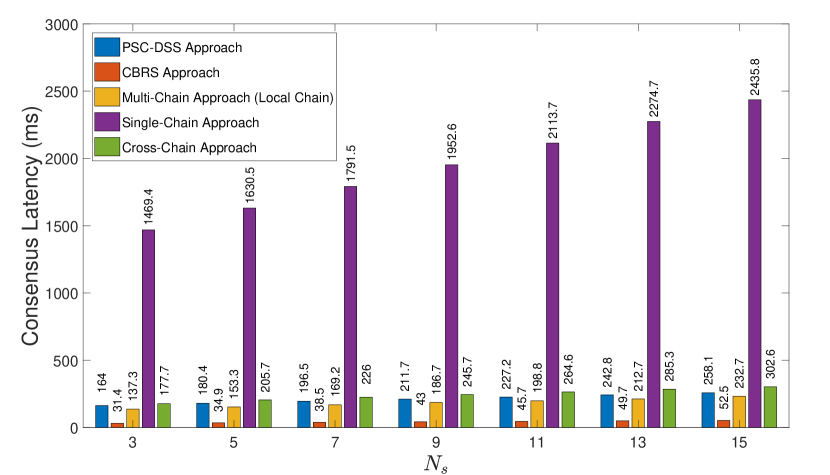
Figure 6: Consensus latency versus $N_{s}$

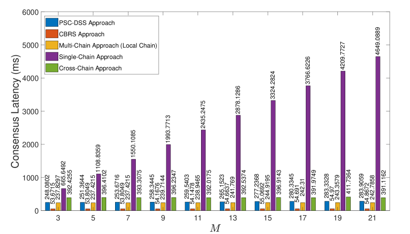
Figure 7: Consensus latency versus $M$

Fig. 7 shows consensus latency versus $M$. We can find that the CBRS and multi-chain approaches are almost unaffected by the change of $M$, because both approaches carry out information dissemination or consensus within their region. However, the slight fluctuations are due to randomly generated base station locations, with a small extent of approximately 2-3 ms. A similar situation occurs in the Cross-Chain approach because this approach perform consensus protocol only in the relevant two regions and transmits cross-region information through satellites. In the single-chain approach, consensus latency increases rapidly with the growth of $M$, as the number of participating nodes also expands significantly. However, although the consensus latency of PSC-DSS increases with $M$ due to the growing number of nodes participating in tier 2 consensus protocol, it still achieves slow latency growth even as $M$ increases, which demonstrates the excellent scalability of PSC-DSS.

V-B2 Efficiency

Fig. 8 shows the transactions per second (TPS) versus the number of regions $M$. For the single-chain approach, as the number of regions $M$ increases, not only does the number of blockchain participants and transactions rise, but the consensus latency also escalates rapidly due to the transmission, propagation, and processing of information across multiple nodes. This results in a difficulty in increasing TPS even in this experiment omitting the network congestion. For the multi-chain approach, TPS decreases with $M$, because allocation record transactions need wait for spectrum allocation transactions to complete a consensus within the region before proceeding to inter-region consensus. Furthermore, as $M$ increases, more nodes need to participate in the global chain’s consensus process, leading to longer consensus latency and consequently reducing TPS. Similarly, the TPS of PSC-DSS slightly decreases with $M$, because the waiting time for candidate blocks submitted by regions to the bootstrapper, as well as the consensus latency among all regulators in tier 2, also increases with $M$. However, PSC-DSS can achieve a relatively stable TPS even as $M$ increases. This is because PSC-DSS consolidates transactions such as spectrum allocation and recording into a single block for consensus, and requires consensus only among nodes within a region and regulators across regions. This approach avoids the need for all nodes to participate in the consensus, and eliminates the waiting times associated with sequential block generation for different transactions.

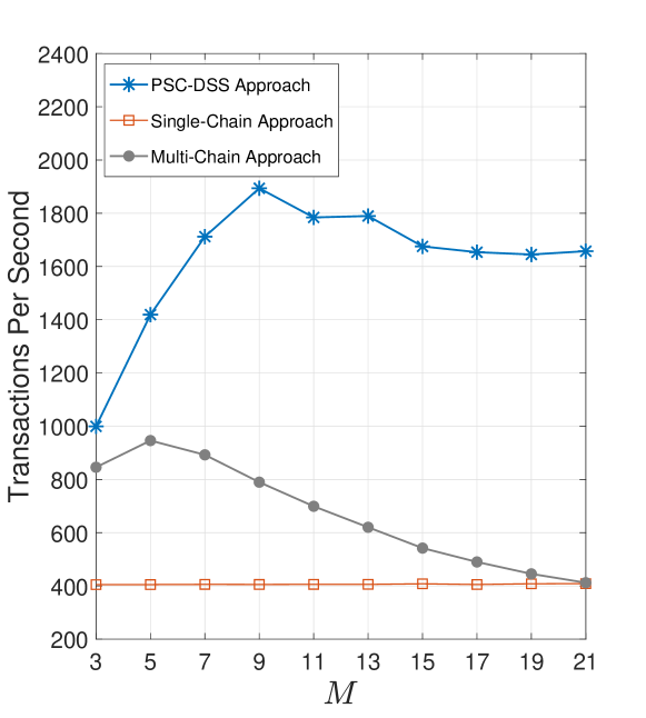
Figure 8: Transactions per second versus $M$

V-B3 Stability

In this experiment, we evaluated the success rate of reaching consensus in dynamic and fixed network topologies with different network parameters, which revealed how many satellite nodes share downlink channels and how many ground nodes share uplink channels for a stable consensus process can be tolerated by the PSC-DSS from the perspective of resource conservation. For dynamic network topology, the number of blockchain participants are various with the density of satellites, where all satellites in ${\cal A}_{DL,vis}$ are treated as blockchain participants and share a same downlink channel. For fixed network topology, the number of blockchain participants are fixed, where the density of satellites is only related with the number of satellites share a same downlink channel. Since this experiment is mainly to explore the effect of satellite-ground wireless network environment on $P_{S}$, we set $P_{out}^{ISL}=P_{out}^{WL}=1$. Besides, the number of regions is set as $M=10$, and the ground nodes as the blockchain participants is set as $N_{g}=15$.

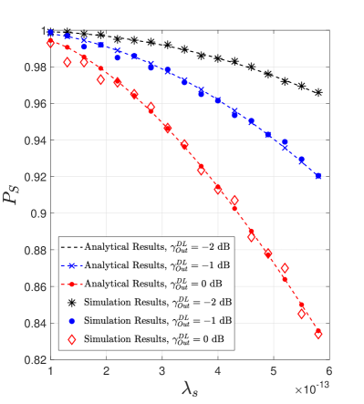
(a) $\lambda_{s}$ versus $\gamma_{out}^{DL}$

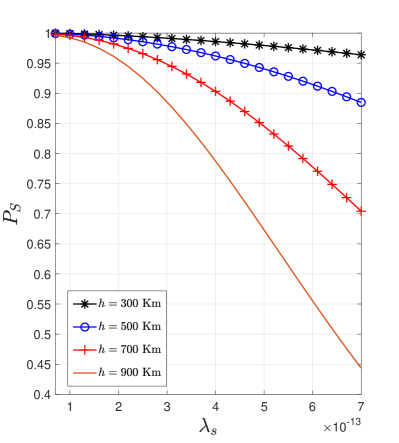
(b) $\lambda_{s}$ versus $h$

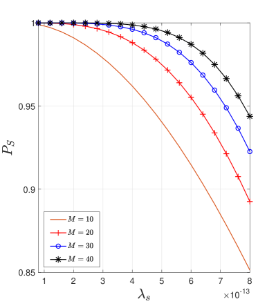
(c) $\lambda_{s}$ versus $M$

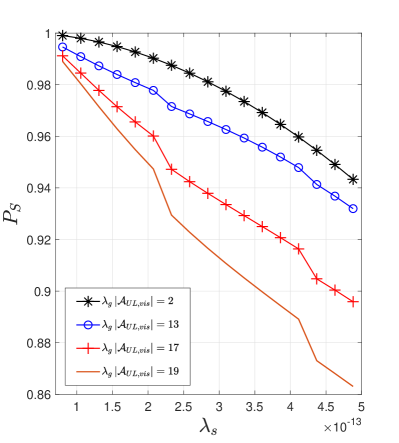
(d) $\lambda_{s}$ versus ${\lambda_{g}}$

Figure 9: Success rate of reaching consensus versus satellite density at different network parameters in the dynamic network topology.

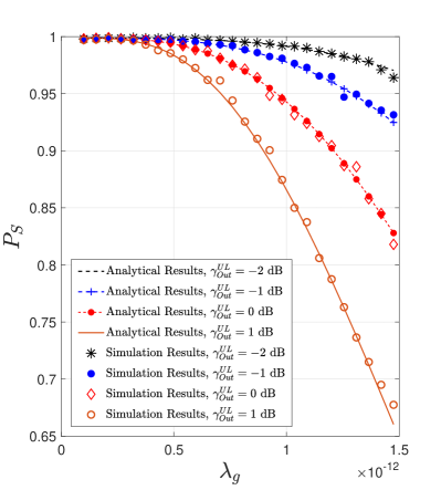
(a) $\lambda_{g}$ versus $\gamma_{out}^{UL}$

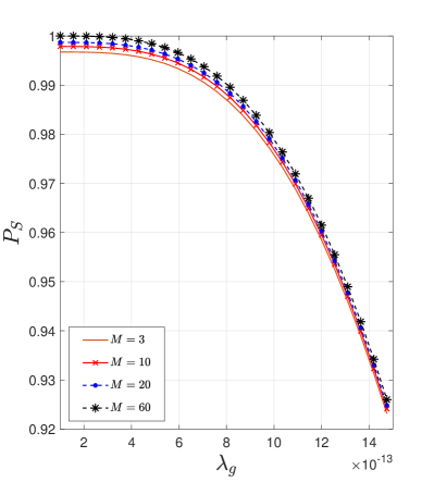
(b) $\lambda_{g}$ versus $M$

Figure 10: Success rate of reaching consensus versus satellite density at different network parameters in the fixed network topology.

TABLE I: The average CPU usage (% core)

	2 $\times$ 4	4 $\times$ 4	4 $\times$ 8	8 $\times$ 4	8 $\times$ 8	8 $\times$ 16	16 $\times$ 8	16 $\times$ 16
Bootstrapper	1.5	3.4	5.5	6.85	6.7	43.85	38.3	53.65
Regulator	2.1	4	5.7	5.2	8.13	17.35	13.5	54.25
Spectrum user	2.5	2.85	4.95	5	5.3	19.8	15.45	49

TABLE II: The average memory usage (MB)

	2 $\times$ 4	4 $\times$ 4	4 $\times$ 8	8 $\times$ 4	8 $\times$ 8	8 $\times$ 16	16 $\times$ 8	16 $\times$ 16
Bootstrapper	54.3	60.95	56.3	59.9	58.25	67.9	67.35	100.05
Regulator	73.7	77.05	76.4	70.6	80.15	84.85	81.4	100.45
Spectrum user	66.4	71.95	70	76.95	74.9	84.8	79.55	98.75

Dynamic Network Topology: Here, every three ground nodes share a uplink channel with uplink SINR threshold set as $\gamma_{out}^{UL}=-1$ dB. From Fig. 9, we can see that $P_{S}$ decreases with $\lambda_{s}$. The higher $\lambda_{s}$, the more satellites share the downlink channel, thus leading to a poorer $P_{f}^{G}$.

Fig. 9(a) first demonstrates the accuracy of the success rate of reaching consensus, where the analytical results are computed from (IV-D), and the simulation results are obtained by independent Monte Carlo trails. Although $P_{S}$ decreases with the downlink SINR threshold $\gamma_{Out}^{DL}$, the black curve shows that PSC-DSS is capable of accommodating 72 satellites (i.e., $\lambda_{s}=6\times 10^{-13}per\;m^{2}$) sharing a downlink channel to reach consensus for spectrum sharing. For the following experiments, we set $\gamma_{Out}^{DL}=-1$ dB.

Fig. 9(b) shows $P_{S}$ decreases with the altitude of satellites, $h=R_{S}-R_{E}$. As the number of satellites in ${\cal A}_{DL,vis}$ increases with altitude $h$, $P_{out}^{DL}$ for ground nodes also increases, thus leading to a higher $P_{f}^{S}$. However, this figure shows that the PSC-DSS can support over 68, 49, 37, and 27 satellites sharing a downlink channel at respective altitudes of 300 Km, 500 Km, 700 Km, and 900 Km.

Fig. 9(c) shows $P_{S}$ increases with the number of regions $M$. When $P_{out}^{DL}$ is large but less than 0.5 (such as $\lambda_{s}=6\times 10^{-13}per\;m^{2}$ for $P_{out}^{DL}=0.3416$), the stability of the system can be enhanced by increasing the number of regions. This is because the increase in the number of regions reduces the probability that more than half of the tier 2 ground nodes will fail, thereby enhancing the success rate of consensus in inter-domain interactions.

Fig. 9(d) shows $P_{S}$ decreases with the number of ground nodes which share a same uplink channel, represented by $\lambda_{g}\left|{\cal A}_{UL,vis}\right|$. From this figure, we can observe that a slight change in $\lambda_{g}\left|{\cal A}_{UL,vis}\right|$ leads to significant changes in $P_{S}$. This is because that the greater $\lambda_{g}\left|{\cal A}_{UL,vis}\right|$, the higher $P_{out}^{UL}$. However, with the increase in $\lambda_{g}$, more satellites experiencing a high $P_{out}^{UL}$ will participate in the consensus process, thus resulting in a rapid decrease in $P_{S}$.

Dynamic Network Topology: In this experiment, every 10 satellites share a downlink with the downlink SINR threshold $\gamma_{Out}^{DL}=-1$ dB, $N_{g}=15$ and $N_{s}=20$. Similar with above results, Fig. 10 shows $P_{S}$ decreases with $\lambda_{g}$ due to the growth in number of ground nodes significantly affect $P_{out}^{UL}$ for satellites.

Fig. 10(a) demonstrates the analytical results exactly matches with the simulation results for all the cases of $\gamma_{Out}^{UL}$. In such case, the block curve shows the PSC-DSS can support over 27 ground nodes share a uplink channel while maintaining system stability. Fig. 10(b) shows that the increasing the number of regions $M$ in this case does not have a significant effect on enhancing system stability $P_{S}$. This is because that, PSC-DSS can maintain a stable consensus process due to the major ground nodes in tier 2 is no faulty when $P_{out}^{DL}$ is small (about 0.1483).

V-C Experiments

In this section, we evaluate the performance of PSC-DSS in terms of computing consumption and memory consumption.

V-C1 Computing Consumption

Table I shows the average CPU usage of the different participants under various number of regions (i.e., $M$) and the number of nodes in a region (i.e., $N_{r}=N_{g}+N_{s}$). We can find that the average CPU usage increases with $M$ and $N_{r}$, attributable to the heightened number of transactions to be executed and the augmentation in communication information to be processed. PSC-DSS starts with CPU usage below 7% for up to 64 nodes, which then rises gradually as it scales to 256 nodes and demonstrates a modest upward trend. Furthermore, we can find that bootstrappers are most affected by the increase in the number of nodes, followed by regulators, and finally spectrum users. This is because that spectrum users only process transactions and performs consensus within a region, while regulators need to execute the both, and bootstrappers need to organize network and coordinate the consensus process in tier 2.

V-C2 Memory Consumption

Table II illustrates the average memory usage for various participants under different configurations of regions and nodes within those regions. From this table, we can find that average memory usage escalates with the increase in the number of nodes. Both regulators and spectrum users exhibit similar patterns in memory consumption. This similarity arises because both types of participants are involved in executing transaction performing consensus process and maintaining a copy of the blockchain ledger. In contrast, the memory usage of the bootstrapper is lower than that of the regulators and spectrum users. The primary reason for this difference is that bootstrappers are not required to execute transaction and maintain a copy of the blockchain ledger. Instead, they only need to store the blocks that have been submitted by each region and boost the consensus process in tier 2. However, as the number of regions increases, so does the number of blocks each bootstrapper needs to manage. This escalation in the number of blocks directly contributes to an increase in memory usage for bootstrappers.

VI Related Works

Recently, efforts have highlighted blockchain’s potential in DSS, focusing on developing smart contracts, blockchain architectures, and consensus mechanisms.

Using smart contract to perform spectrum sharing schemes is a common approach. Jiang et al. [30] propose a smart contract-enabled permissioned blockchain-based dynamic spectrum acquisition scheme. Boateng et al. [31] design smart contracts to perform decentralized spectrum trading. Ayepah-Mensah et al. [32] employ smart contracts to execute resource allocation and trading process among RANs. Xu et al. [33] record the spectrum auction results into a smart contract. Although these efforts enable DSS efficiently, they require all participants to follow a conventional architecture and a unified spectrum sharing scheme. As participant numbers grow, these efforts inevitably face significant bottlenecks due to limited scalability and constrained flexibility in meeting the dynamic and varied needs of participants.

Aiming to improve the scalability of blockchain-based DSS systems, an emerging trend is to establish new architectures incorporating tiered and sharded features. Hu et al. [34] introduce a two-tier hierarchical blockchain architecture for DSS, consisting of a global chain in tier 1 and multiple local chains in tier 2. Local chains are updated to the global chain at a fixed or a dynamic frequency. Xiao et al. [14, 7] propose a blockchain-based decentralized SAS architecture, with a global chain used for spectrum regulatory tasks and several local chains for automating spectrum access assignment. Also, the state of local chains is updated on global chain at a fixed frequency. However, these approaches cannot realize the global real-time synchronization of spectrum information. Grissa et al. [6] present a trustworthy framework for SAS. In each cluster, secondary users maintain a local blockchain and validators maintain a global blockchain. Members within clusters hold a light copy of the global blockchain containing the latest status of the system. However, these efforts are not optimal for SANs because they depend on a multi-chain structure and require additional operations for cross-chain transactions, demanding significant resources from participants.

In order to reduce the overhead of blockchain in DSS, many efforts have focused on developing innovative consensus mechanisms. Zhu et al. [5] integrate the computation of the deep reinforcement learning-based method for solving the winner determination problem with the proof-of-work consensus mechanism. Fernando et al. [35] propose a proof-of-sense consensus mechanism, where the spectrum first sensor to successfully recovers a secret key transmitted randomly in a frequency band is rewarded. Ye et al. [36] introduce a proof-of-trust consensus mechanism that links participants’ trust values with mining difficulty to reduce overhead in DSS. Notwithstanding the progress, these efforts still face challenges in terms of constrained flexibility and weak compatibility, and thus failing to be effectively applied in the involving SANs.

To analyze the performance of blockchain in wireless networks, theoretical models are required. Sun et al. [15] establish an analytical model for the blockchain-enabled wireless system. Xu et al. [37] investigate the security performance of wireless blockchain networks in the presence of malicious jamming for RAFT consensus mechanism. Wang et al. [29] analyze the probability of forking events in the intra-shard-transactions by considering the fading channel. However, the existing studies is for terrestrial networks and can not be directly applied in SANs due to the differences between terrestrial networks and SANs in terms of channel model, spatial distribution, and coverage condition.

To face the aforementioned challenges, we construct a blockchain-based architecture with a two-tier and multi-region design, however, it requires maintaining only one blockchain. Then, a spectrum-consensus integrated mechanism is proposed to enhance DSS efficiency and enable regions to dynamically innovate spectrum sharing schemes. Moreover, a theoretical framework which considers the unsteady and complex features of SANs is built to analyze the stability of PSC-DSS.

VII Conclusion

This work proposes a partitioned, self-governed, and customized dynamic spectrum sharing approach for spectrum sharing between satellite access networks and terrestrial access networks. First, a sharded and tiered architecture is established to allows various regions to manage spectrum autonomously while jointly maintaining a single blockchain ledger. Then, a spectrum-consensus integrated mechanism is designed to enable regions to parallelly conduct DSS transactions and dynamically innovate spectrum sharing schemes without affecting others. Finally, a theoretical framework using stochastic geometry is derived to justify the stability performance of the proposed approach. Simulations and experiments are conducted to validate the advantageous performance of PSC-DSS in terms of low-overhead, high efficiency, and robust stability.

Appendix A

In PSC-DSS, the intra-region interaction tolerates no more than $\left\lfloor{\frac{N_{r}}{3}}\right\rfloor$ (i.e., $N_{r}=N_{s}+N_{g}$)faulty nodes (including satellites and ground nodes) based on PBFT consensus protocol (denoted as EVENT A), and the inter-regin interaction requires no more than $\left\lfloor{\frac{M}{2}}\right\rfloor$ faulty regulators to commit a block (denoted as EVENT B). Furthermore, EVENT A includes two case: the regulator is not faulty (denoted as EVENT A0), and the regulator is faulty (denoted as EVENT A1). However, EVENT A and EVENT B are not independent. If a regulator in intra-region interaction is faulty, it will affect the the consensus reaching process in the inter-region interaction. In such case, we have

$$P_{S}=\sum\limits_{i=0}^{\left\lfloor{\frac{{{N_{r}}}}{3}}\right\rfloor}{\Pr\left({A0}\right)\times\Pr\left({A=i\left|{A0}\right.}\right)\times}\Pr\left({B\left|{A=i,A0}\right.}\right)$$

$$+\sum\limits_{i=1}^{\left\lfloor{\frac{{{N_{r}}}}{3}}\right\rfloor}{\Pr\left({A1}\right)\times\Pr\left({A=i\left|{A1}\right.}\right)}\Pr\left({B\left|{A=i,A1}\right.}\right),$$ (27)

Here, $\Pr(A0)=1-P_{f}^{G}$ and $\Pr(A1)=P_{f}^{G}$, $\Pr\left({A=i\left|{A1}\right.}\right)$ and $\Pr\left({A=i\left|{A0}\right.}\right)$ presents the probabilities that there are $i$ faulty nodes in intra-region interaction under the conditions that the regulator is faulty and not faulty, respectively. These probabilities are given as

$$\Pr\left({A=i\left|{A0}\right.}\right)=\sum\limits_{n=0}^{\min(i,{N_{g}}-{\rm{1}})}{P_{n0}},$$ (28)

and

$$\Pr\left({A=i\left|{A1}\right.}\right)=\sum\limits_{n=1}^{\min(i,{N_{g}})}{P_{n1}},$$ (29)

with

$${P_{n0}} =C_{{N_{g}}-1}^{n}{\left({P_{f}^{G}}\right)^{n}}{\left({1-P_{f}^{G}}\right)^{{N_{g}}-1-n}}\times{\textbf{1}_{\left\{{i-n<{N_{s}}}\right\}}}$$

$$\;\;\;\;\times C_{{N_{s}}}^{i-n}{\left({P_{f}^{S}}\right)^{i-n}}{\left({1-P_{f}^{S}}\right)^{{N_{s}}-\left({i-n}\right)}},$$ (30)

$${P_{n{\rm{1}}}} =C_{{N_{g}}-{\rm{1}}}^{n-{\rm{1}}}{\left({P_{f}^{G}}\right)^{n-1}}{\left({1-P_{f}^{G}}\right)^{{N_{g}}-n}}\times{\textbf{1}_{\left\{{i-n<{N_{s}}}\right\}}}$$

$$\;\;\;\;\times C_{{N_{s}}}^{i-n}{\left({P_{f}^{S}}\right)^{i-n}}{\left({1-P_{f}^{S}}\right)^{{N_{s}}-\left({i-n}\right)}},$$ (31)

where ${\textbf{1}_{\left\{.\right\}}}$ is the indicator function.

$\Pr\left({B\left|{A=i,A0}\right.}\right)$ and $\Pr\left({B\left|{A=i,A1}\right.}\right)$ indicates the probabilities of EVENT B occurring under the conditions that there are already $i$ faulty nodes in intra-region interaction, with a faulty regulator and without a faulty regulator, respectively. The expressions for these probabilities are given as

$$\Pr\left({B\left|{A=i,A0}\right.}\right)={\sum\limits_{j=0}^{\left\lfloor{\frac{M}{2}}\right\rfloor}{P_{j}}},$$ (32)

and

$$\Pr\left({B\left|{A=i,A1}\right.}\right)={\sum\limits_{j=0}^{\left\lfloor{\frac{M}{2}}\right\rfloor-1}{P_{j}}},$$ (33)

with

$$P_{j}={C_{M-1}^{j}{{\left({P_{f}^{G}}\right)}^{j}}{{\left({1-P_{f}^{G}}\right)}^{M-1-j}}}.$$ (34)

Thus, the expression of $P_{S}$ can be given as (IV-B).

Appendix B Proof of Lemma 1

Since the locations of satellites are distributed according to homogeneous SPPP with density, the number of satellites in ${{\cal A}_{DL,vis}}$ follows Poisson random variable with mean $\lambda_{s}\left|{{{\cal A}_{DL,vis}}}\right|$. Therefore, the probability that there is at least one satellite in ${{{\cal A}_{DL,vis}}}$ can be computed by

$$\Pr\left({\Phi\left({{{\cal A}_{DL,vis}}}\right)>0}\right) =1-\Pr\left({\Phi_{S}\left({{{\cal A}_{DL,vis}}}\right)=0}\right)$$

$$=1-\exp\left(-\lambda_{s}\left|{{{\cal A}_{DL,vis}}}\right|\right),$$ (35)

Similarly, the probability that there is at least one ground node in ${{{\cal A}_{UL,vis}}}$ can be computed by

$$\Pr\left({\Phi\left({{{\cal A}_{UL,vis}}}\right)>0}\right) =1-\Pr\left({\Phi_{G}\left({{{\cal A}_{UL,vis}}}\right)=0}\right)$$

$$=1-\exp\left(-\lambda_{g}\left|{{{\cal A}_{UL,vis}}}\right|\right).$$ (36)

Based on Archimedes’ Hat-Box Theorem [20], $\left|{{{\cal A}_{DL,vis}}}\right|$, and $\left|{{{\cal A}_{UL,vis}}}\right|$, respectively, are given as

$$\left|{{{\cal A}_{DL,vis}}}\right|=2\pi R_{S}H_{DL}(D_{DL,0}^{\max}),$$ (37)

and

$$\left|{{{\cal A}_{UL,vis}}}\right|=2\pi R_{E}H_{UL}(\varphi_{\max}),$$ (38)

where ${D_{DL,0}^{\max}}=\sqrt{{{\left({R_{E}\sin{\theta_{\min}}}\right)}^{2}}+R_{S}^{2}-R_{E}^{2}}-R_{E}\sin{\theta_{\min}}$ is the maximum distance between $G_{DL,0}$ and satellites in downlink communications. Here, $H_{DL}(D_{DL,0})$ is the height of spherical crown shown in Fig. 3(a), and $H_{UL}(\varphi)$ is the height of spherical crown shown in Fig. 3(b), which are given by $H_{DL}(D_{DL,0})=\frac{{D_{DL,0}^{2}+2{R_{E}}{R_{S}}-R_{E}^{2}-R_{S}^{2}}}{{2{R_{E}}}}$ and $H_{UL}(\varphi)=R_{E}\left({1-\cos{\varphi}}\right)$.

By substituting (37) and (38) into (B) and (B), respectively, the proof is completed.

Appendix C Proof of Lemma 2

The conditional cumulative density function (CDF) of $D_{DL,0}$, $F_{D_{DL,0}}(d_{DL,0})$, is characterized as $\Pr\left({D_{DL,0}\leq d_{DL,0}\left|{\Phi\left({{{\cal A}_{DL,vis}}}\right)>0}\right.}\right)$, indicating that the distance between $G_{DL,0}$ and $S_{DL,0}$ is less than $d_{DL,0}$ conditioned that at least more than one satellite exists in ${\cal A}_{DL,vis}$. Following derivations in [20], the $F_{D_{DL,0}}(d_{DL,0})$ is given by

$${F_{{D_{DL,0}}}}\left({{d_{DL,0}}}\right)=\Pr\left({{D_{DL,0}}\leq{d_{DL,0}}\left|{{\Phi_{S}}\left({{{\cal A}_{DL,vis}}}\right)>0}\right.}\right)$$

$$=1-\Pr\left({{D_{DL,0}}>{d_{DL,0}}\left|{{\Phi_{S}}\left({{{\cal A}_{DL,vis}}}\right)>0}\right.}\right)$$

$$=1-{\left[{1-\exp\left({-{\lambda_{s}}\left|{{{\cal A}_{DL,vis}}}\right|}\right)}\right]^{-1}}$$

$$\;\;\;\;\;\;\;\times\exp\left({-{\lambda_{s}}\left|{{{{\cal A}^{\prime}}_{DL,vis}}\left({{d_{DL,0}}}\right)}\right|}\right)$$

$$\;\;\;\;\;\;\;\times\left[{1-\exp\left({-{\lambda_{s}}\left({\left|{{{\cal A}_{DL,vis}}}\right|-\left|{{{{\cal A}^{\prime}}_{DL,vis}}\left({{d_{DL,0}}}\right)}\right|}\right)}\right)}\right]$$

$$\mathop{=}\limits^{\left(a\right)}\frac{{1-\exp\left({-\pi{\lambda_{s}}{R_{S}}\frac{{d_{DL,0}^{2}+2{R_{E}}{R_{S}}-R_{E}^{2}-R_{S}^{2}}}{{{R_{E}}}}}\right)}}{{1-\exp\left({-\pi{\lambda_{s}}{R_{S}}{\frac{{{{\left({D_{DL,0}^{\max}}\right)}^{\rm{2}}}+2{R_{E}}{R_{S}}-R_{E}^{2}-R_{S}^{2}}}{{{R_{E}}}}}}\right)}},$$ (39)

where (a) follows from (37) and $\left|{{{{\cal A}^{\prime}}_{DL,vis}}\left({{d_{DL,0}}}\right)}\right|=2\pi R_{S}H_{DL}(d_{DL,0})$.

Similarly, the conditional CDF of $D_{UL,0}$, $F_{D_{UL,0}}(d_{UL,0})$, is characterized as $\Pr\left({D_{UL,0}\leq d_{UDL,0}\left|{\Phi\left({{{\cal A}_{UL,vis}}}\right)>0}\right.}\right)$, indicating that the distance between $S_{UL,0}$ and $G_{UL,0}$ is less than $d_{UL,0}$ conditioned that at least more than one ground node exists in ${\cal A}_{UL,vis}$. The $F_{D_{UL,0}}(d_{UL,0})$ is given by

$${F_{D_{UL,0}}}\left({{d_{UL,0}}}\right)=\Pr\left({{D_{DL,0}}\leq{d_{DL,0}}\left|{{\Phi_{G}}\left({{{\cal A}_{UL,vis}}}\right)>0}\right.}\right)$$

$$=1-\Pr\left({{D_{UL,0}}>{d_{UL,0}}\left|{{\Phi_{G}}\left({{{\cal A}_{UL,vis}}}\right)>0}\right.}\right)$$

$$=\frac{{1-\exp\left({-{\lambda_{g}}\left|{{{{\cal A}^{\prime}}_{UL,vis}}\left({\varphi({d_{UL,0}})}\right)}\right|}\right)}}{{1-\exp\left({-{\lambda_{\rm{g}}}\left|{{{\cal A}_{UL,vis}}}\right|}\right)}}$$

$$\mathop{=}\limits^{\left(b\right)}\frac{{1-\exp\left({-\pi{\lambda_{g}}{R_{E}}\frac{{d_{UL,0}^{2}+2{R_{E}}{R_{S}}-R_{E}^{2}-R_{S}^{2}}}{{{R_{S}}}}}\right)}}{{1-\exp\left({-\pi{\lambda_{g}}{R_{E}}{\frac{{{{\left({D_{UL,0}^{\max}}\right)}^{\ {2}}}+2{R_{E}}{R_{S}}-R_{E}^{2}-R_{S}^{2}}}{{{R_{S}}}}}}\right)}},$$ (40)

where (b) follows from (38) with $\cos\varphi_{\max}={\frac{{R_{E}^{2}+R_{S}^{2}-(D_{UL,0}^{\max})^{2}}}{{2{R_{S}}{R_{E}}}}}$, and $\left|{{{{\cal A}^{\prime}}_{UL,vis}}\left({{d_{UL,0}}}\right)}\right|=2\pi R_{E}H_{UL}(\varphi(d_{UL,0}))$ with $\varphi=\arccos\left({\frac{{R_{E}^{2}+R_{S}^{2}-d_{UL,0}^{2}}}{{2{R_{S}}{R_{E}}}}}\right)$.

By taking derivative with respect to the variables in $F_{D_{DL,0}}(d_{DL,0})$ and $F_{D_{UL,0}}(d_{UL,0})$, the conditional PDF of ${D_{DL,0}}$ and ${D_{UL,0}}$ are computed as

$${f_{{D_{DL,0}}}}\left({{d_{DL,0}}}\right) ={\xi_{DL}}{d_{DL,0}}\exp\left({-\pi{\lambda_{s}}\frac{{{R_{S}}}}{{{R_{E}}}}d_{DL,0}^{2}}\right),$$ (41)

and

$${f_{{D_{UL,0}}}}\left({{d_{UL,0}}}\right) ={{\xi_{UL}}{d_{UL,0}}\exp\left({-\pi{\lambda_{g}}\frac{{{R_{E}}}}{{{R_{S}}}}d_{UL,0}^{2}}\right)},$$ (42)

respectively, where $d_{DL,0}\in\left[{{D_{DL,0}^{min}},{D_{DL,0}^{max}}}\right]$, $d_{UL,0}\in\left[{{D_{UL,0}^{min}},{D_{UL,0}^{max}}}\right]$, ${\xi_{DL}}$ and ${\xi_{UL}}$ are given by

$${\xi_{DL}}=\frac{{\frac{{2\pi{\lambda_{s}}{R_{s}}}}{{{R_{E}}}}\exp\left({-\pi{\lambda_{s}}{R_{S}}\frac{{2{R_{E}}{R_{S}}-R_{E}^{2}-R_{S}^{2}}}{{{R_{E}}}}}\right)}}{{1-\exp\left({-\pi{\lambda_{s}}{R_{S}}\frac{{{{\left({D_{DL,0}^{\max}}\right)}^{\rm{2}}}+2{R_{E}}{R_{S}}-R_{E}^{2}-R_{S}^{2}}}{{{R_{E}}}}}\right)}},$$ (43)

and

$${\xi_{UL}}=\frac{\frac{{2\pi{\lambda_{g}}{R_{E}}}}{{{R_{S}}}}{\exp\left({-\pi{\lambda_{g}}{R_{E}}\frac{{2{R_{E}}{R_{S}}-R_{E}^{2}-R_{S}^{2}}}{{{R_{S}}}}}\right)}}{{1-\exp\left({-\pi{\lambda_{g}}{R_{E}}\frac{{{{\left({D_{UL,0}^{\max}}\right)}^{{2}}}+2{R_{E}}{R_{S}}-R_{E}^{2}-R_{S}^{2}}}{{{R_{S}}}}}\right)}}.$$ (44)

This completes the proof.

Appendix D Proof of Lemma 3

Following the definition of the conditional aggregated interference at $G_{DL,0}$ presented as ${{\bar{I}}_{G}}$, ${\Phi_{S}^{{}^{\prime}}}={\Phi_{S}}\cap{{\cal A}_{DL,vis}}\backslash{\cal A}_{DL,vis}^{{}^{\prime}}\left({{d_{DL,0}}}\right)$ denotes the area on the spherical cap outside ${\cal A}{{}^{{}^{\prime}}_{DL,vis}}\left({{d_{DL,0}}}\right)$. Thus, the Laplace transform of ${{\bar{I}}_{G}}$ is computed by

$${{\cal L}_{{{\bar{I}}_{G}}}}\left(s\right)={\mathbb{E}_{{{\bar{I}}_{G}}}}\left[{\left.{{e^{-s{{\bar{I}}_{G}}}}}\right|{D_{DL,0}=d_{DL,0}},{\Phi_{s}}\left({{\cal A}{{}_{DL,vis}}}\right)>0}\right]$$

$$\mathop{=}\limits^{\left(a\right)}{\mathbb{E}_{{\Phi_{S}}\left({{\cal A}{{}_{DL,vis}}}\right)}}\left[{\prod\limits_{i\in{{\Phi}_{S}^{{}^{\prime}}}}{{\mathbb{E}_{{{\left|h\right|}^{2}}}}\left[{\exp\left({-s{{\bar{g}}_{DL}}{{\left|h\right|}^{2}}d_{DL,i}^{-2}}\right)}\right]}}\right]$$

$$\mathop{=}\limits^{\left(b\right)}\exp\left({-{\lambda_{s}}\int_{d\in\bar{\cal A}{{}_{DL,vis}}}{\rm{d}}\left({\left|\bar{\cal A}{{}_{DL,vis}}\right|}\right)}\right)$$

$$-\exp\left({-{\lambda_{s}}\int_{d\in\bar{\cal A}{{}_{DL,vis}}}{{\mathbb{E}_{{{\left|h\right|}^{2}}}}\left({e^{{-s{{\bar{g}}_{DL}}{{\left|h\right|}^{2}}d^{-2}}}}\right){\rm{d}}\left({\left|\bar{\cal A}{{}_{DL,vis}}\right|}\right)}}\right)$$

$$\mathop{=}\limits^{\left(c\right)}\exp\left({-2\pi{\lambda_{s}}\frac{{{R_{S}}}}{{{R_{E}}}}\int_{{d_{DL,0}}}^{D_{DL,0}^{\max}}{\left({1-{\mathbb{E}_{{{\left|h\right|}^{2}}}}\left({e^{{-s{{\bar{g}}_{DL}}{{\left|h\right|}^{2}}d^{-2}}}}\right)}\right)d{\rm{d}}d}}\right)$$

$$\mathop{=}\limits^{\left(d\right)}\exp\left({-2\pi{\lambda_{s}}\frac{{{R_{S}}}}{{{R_{E}}}}\int_{{d_{DL,0}}}^{D_{DL,0}^{\max}}{d\left({1-\frac{1}{{{{\left({s{{\bar{g}}_{DL}}d^{-2}\beta+1}\right)}^{\alpha}}}}}\right){\rm{d}}d}}\right)$$

$$\mathop{=}\limits^{\left(e\right)}\exp\left({-\pi{\lambda_{s}}\frac{{{R_{S}}}}{{{R_{E}}}}\left({{{\left({D_{DL,0}^{\max}}\right)}^{2}}-d_{DL,0}^{2}}\right)}\right)$$

$$\times\exp\left({\pi{\lambda_{s}}\frac{{{R_{S}}}}{{{R_{E}}}}\int_{\frac{{d_{DL,0}^{2}}}{{s{{\bar{g}}_{DL}}\beta}}}^{\frac{{{{\left({D_{DL,0}^{\max}}\right)}^{2}}}}{{s{{\bar{g}}_{DL}}\beta}}}{\left({\frac{1}{{{{\left({{t^{-1}}+1}\right)}^{\alpha}}}}}\right){\rm{d}}\left({s{{\bar{g}}_{DL}}\beta t}\right)}}\right)$$

$$\mathop{=}\limits^{\left(f\right)}\exp\left({-\pi{\lambda_{s}}\frac{{{R_{S}}}}{{{R_{E}}}}\left({{{\left({D_{DL,0}^{\max}}\right)}^{2}}-d_{DL,0}^{2}}\right)}\right)$$

$$\times\exp\left({\pi{\lambda_{s}}\frac{{{R_{S}}}}{{{R_{E}}}}\frac{{{{\left({D_{DL,0}^{\max}}\right)}^{2\left({\alpha+1}\right)}}}}{{{\left({s{{\bar{g}}_{DL}}\beta}\right)}^{\alpha}(\alpha+1)}}{\times{J\left({s,{{\bar{g}}_{DL}},D_{DL,0}^{\max}}\right)}}}\right)$$

$$\div\exp\left({\pi{\lambda_{s}}\frac{{{R_{S}}}}{{{R_{E}}}}\frac{{d_{DL,0}^{2\left({\alpha+1}\right)}}}{{{\left({s{{\bar{g}}_{DL}}\beta}\right)}^{\alpha}(\alpha+1)}}{{J\left({s,{{\bar{g}}_{DL}},d_{DL,0}}\right)}}}\right)$$ (45)

where (a) follows from the i.i.d. distribution of ${\left|{{h_{DL,i}}}\right|^{2}}$, (b) follows from the probability generating functional (PGFL) of the SPPP and ${\bar{\cal A}{{}_{DL,vis}}}={{\cal A}{{}_{DL,vis}}\backslash{\cal A}{{}^{{}^{\prime}}_{DL,vis}}\left({{d_{DL,0}}}\right)}$, (c) comes from $\frac{{\partial\left|{\bar{\cal A}{{}_{DL,vis}}}\right|}}{{\partial d_{DL,0}}}=2\pi\frac{{{R_{S}}}}{{{R_{E}}}}{d_{DL,0}}$, (d) comes from the Laplace transform of ${{\left|h\right|}^{2}}$ that is ${\mathbb{E}_{{{\left|h\right|}^{2}}}}\left({{e^{-s{{\bar{g}}_{DL}}{{\left|h\right|}^{2}}d^{-2}}}}\right)={{\cal L}_{{{\left|h\right|}^{2}}}}\left({s{{\bar{g}}_{DL}}d^{-2}}\right)=\frac{1}{{{{\left({s{{\bar{g}}_{DL}}d^{-2}\beta+1}\right)}^{\alpha}}}}$, (e) is the change of variable ${t=\left({s{{\bar{g}}_{DL}}\beta}\right)^{-1}}d^{2}$, and (f) comes from $\int_{0}^{u}{\frac{{{x^{\mu-1}}dx}}{{{{(1+\beta x)}^{\nu}}}}}=\frac{{{u^{\mu}}}}{\mu}{\times_{2}}{F_{1}}\left({\nu,\mu;1+\mu;-\beta u}\right)$, and the Gaussian hypergeometric function ${}_{2}{F_{1}}\left({.,.;.;.}\right)$ is expressed by $J\left({\varpi,\tau,\upsilon}\right){=_{2}}{F_{1}}\left({\alpha,\alpha+1;2+\alpha;-\frac{{{\upsilon^{2}}}}{{\varpi\tau\beta}}}\right)$.

Similarly, according to the definition of the conditional aggregated interference ${{\bar{I}}_{S}}$ at $S_{UL,0}$, ${\Phi_{G}^{{}^{\prime}}}={\Phi_{G}}\cap{{\cal A}_{UL,vis}}\backslash{\cal A}_{UL,vis}^{{}^{\prime}}\left({{d_{UL,0}}}\right)$ denotes the area on the spherical cap outside ${\cal A}{{}^{{}^{\prime}}_{UL,vis}}\left({{d_{UL,0}}}\right)$. Thus, the Laplace transform of ${{\bar{I}}_{S}}$ is computed by

$${{\cal L}_{{{\bar{I}}_{S}}}}\left(s\right)={\mathbb{E}_{{{\bar{I}}_{S}}}}\left[{\left.{{e^{-s{{\bar{I}}_{S}}}}}\right|{D_{UL,0}=d_{UL,0}},{\Phi_{G}}\left({{\cal A}{{}_{UL,vis}}}\right)>0}\right]$$

$$=\mathbb{E}{{}_{{\Phi_{G}}\left({{\cal A}{{}_{UL,vis}}}\right),{{\left|{{h_{UL,j}}}\right|}^{2}}}}\left[{\exp\left({-\sum\limits_{j\in{{{\Phi}_{G}^{{}^{\prime}}}}}{s{{\bar{g}}_{UL}}{{\left|{{h_{UL,j}}}\right|}^{2}}d_{DL,j}^{-2}}}\right)}\right]$$

$$=\exp\left({-\pi{\lambda_{g}}\frac{{{R_{E}}}}{{{R_{S}}}}\left({{{\left({D_{UL,0}^{\max}}\right)}^{2}}-d_{UL,0}^{2}}\right)}\right)$$

$$\times\exp\left({\pi{\lambda_{g}}\frac{{{R_{E}}}}{{{R_{S}}}}\frac{{{{\left({D_{UL,0}^{\max}}\right)}^{2\left({\alpha+1}\right)}}}}{{{\left({s{{\bar{g}}_{UL}}\beta}\right)}^{\alpha}(\alpha+1)}}{\times{J\left({s,{{\bar{g}}_{UL}},D_{UL,0}^{\max}}\right)}}}\right)$$

$$\div\exp\left({\pi{\lambda_{g}}\frac{{{R_{E}}}}{{{R_{S}}}}\frac{{d_{UL,0}^{2\left({\alpha+1}\right)}}}{{{\left({s{{\bar{g}}_{UL}}\beta}\right)}^{\alpha}(\alpha+1)}}{{J\left({s,{{\bar{g}}_{UL}},d_{UL,0}}\right)}}}\right)$$ (46)

This completes the proof.

Appendix E

Based on the expression of (IV-C), the outage probability of $G_{DL,0}$ conditioned on $\Phi_{S}({\cal A}_{DL,vis})>0$ is computed by

$$P_{out}^{DL}\left({\gamma\left|{\Phi_{S}\left({{{\cal A}_{DL,vis}}}\right)>0}\right.}\right)$$

$$={\mathbb{E}_{{D_{DL,0}}}}\left[{{\mathbb{E}_{{{\bar{I}}_{G}}}}\left[{\Pr\left[{{{\left|{{h_{DL,0}}}\right|}^{2}}<\gamma\left({\bar{\sigma}_{G}^{2}+{{\bar{I}}_{G}}}\right)D_{DL,0}^{2}}\right.}\right.}\right.$$

$$\times\left.{\left.{\left.{\left|{D_{DL,0},\Phi_{S}\left({{{\cal A}_{DL,vis}}}\right)>0,{{\bar{I}}_{G}}}\right.}\right]}\right]}\right]$$

$$\mathop{=}\limits^{\left(a\right)}1-{\mathbb{E}_{{D_{DL,0}}}}\left[{\exp\left({-{\beta^{-1}}\bar{\sigma}_{G}^{2}\gamma D_{DL,0}^{2}}\right)}\right.$$

$$\times{\mathbb{E}_{{{\bar{I}}_{G}}}}\left[{{e^{-{\beta^{-1}}\gamma D_{DL,0}^{2}{{\bar{I}}_{G}}}}}\right.\sum\limits_{m=0}^{\alpha-1}{\frac{{{{\left({{\beta^{-1}}\gamma D_{DL,0}^{2}\left({\bar{\sigma}_{G}^{2}+{{\bar{I}}_{G}}}\right)}\right)}^{m}}}}{{m!}}}$$

$$\times\left|{\left.{\left.{D_{DL,0},\Phi_{S}\left({{{\cal A}_{DL,vis}}}\right)>0,{{\bar{I}}_{G}}}\right]}\right]}\right.$$

$$\mathop{=}\limits^{\left(b\right)}1-{\mathbb{E}_{{D_{DL,0}}}}\left[{\exp\left({-{\beta^{-1}}\bar{\sigma}_{G}^{2}\gamma D_{DL,0}^{2}}\right)}\right]$$

$$\times{\mathbb{E}_{{D_{DL,0}}}}\left[{\sum\limits_{m=0}^{\alpha-1}{{\mathbb{E}_{{{\bar{I}}_{G}}}}\left[{{e^{-{\beta^{-1}}\gamma D_{DL,0}^{2}{{\bar{I}}_{G}}}}\times\frac{{{{\left({sD_{DL,0}^{2}}\right)}^{m}}}}{{m!}}}\right.}}\right.$$

$$\times\left.{\left.{\left.{\sum\limits_{k=0}^{m}{C_{m}^{k}{{\left({\bar{\sigma}_{G}^{2}}\right)}^{m-k}}{{\left({{{\bar{I}}_{G}}}\right)}^{k}}}}\right|D_{DL,0},\Phi_{S}\left({{{\cal A}_{DL,vis}}}\right)>0,{{\bar{I}}_{G}}}\right]}\right]$$

$$\mathop{=}\limits^{\left(c\right)}1-{\mathbb{E}_{{D_{DL,0}}}}\left[{\exp\left({-{\beta^{-1}}\bar{\sigma}_{G}^{2}\gamma D_{DL,0}^{2}}\right)}\right]$$

$$\times{\mathbb{E}_{{D_{DL,0}}}}\left[{\sum\limits_{m=0}^{\alpha-1}{\left[{\frac{{{{\left({sD_{DL,0}^{2}}\right)}^{m}}}}{{m!}}\sum\limits_{k=0}^{m}{C_{m}^{k}{{\left({\bar{\sigma}_{G}^{2}}\right)}^{m-k}}}}\right.}}\right.$$

$$\times\left.{\left.{\left.{{{\left({-1}\right)}^{k}}\frac{{{{\rm{d}}^{k}}{{\cal L}_{{{\bar{I}}_{G}}}}\left({sD_{DL,0}^{2}}\right)}}{{{\rm{d}}{{\left({sD_{DL,0}^{2}}\right)}^{k}}}}}\right|D_{DL,0},\Phi_{S}\left({{{\cal A}_{DL,vis}}}\right)>0,{{\bar{I}}_{G}}}\right]}\right]$$

where (a) follows the CDF of ${\left|h\right|}^{2}$ that is given as ${F_{{{\left|h\right|}^{2}}}}\left(x\right)=\Pr\left({{{\left|h\right|}^{2}}\leq x}\right)=1-\exp\left({-\frac{x}{\beta}}\right)\sum\limits_{m=0}^{\alpha-1}{\frac{{{{\left({\frac{x}{\beta}}\right)}^{m}}}}{{m!}}}$, (b) is the change of variable $s={\beta^{-1}}\gamma$ and ${\left({a+b}\right)^{m}}=\sum\limits_{k=0}^{m}{C_{m}^{k}{a^{m-k}}{b^{k}}}$, (c) follows ${\mathbb{E}_{x}}\left[{{{\left(x\right)}^{k}}{e^{-sx}}}\right]={\left({-1}\right)^{k}}\frac{{{{\rm{d}}^{k}}{{\cal L}_{x}}\left(s\right)}}{{{\rm{d}}{s^{k}}}}$. Here, the PDF of $D_{DL,0}$ is given in Lemma 2, and the Laplace transform of ${\bar{I}}_{G}$ is given in Lemma 3.

Similarly, based on the expression of (IV-C), the outage probability of $S_{UL,0}$ conditioned on $\Phi_{G}({\cal A}_{UL,vis})>0$ is computed by

$$P_{out}^{UL}\left({\gamma\left|{\Phi_{G}\left({{{\cal A}_{UL,vis}}}\right)>0}\right.}\right)$$

$$=1-\int_{{d_{{}_{UL,}0}}>0}{e^{{-{\beta^{-1}}\bar{\sigma}_{S}^{2}\gamma d_{UL,0}^{2}}}{f_{{D_{UL,0}}}}\left({{d_{UL,0}}}\right){\rm{d}}{d_{UL,0}}}$$

$$\times\int_{{d_{{}_{UL,}0}}>0}{\sum\limits_{m=0}^{\alpha-1}{\left[{\frac{{{{\left({sD_{UL,0}^{2}}\right)}^{m}}}}{{m!}}\sum\limits_{k=0}^{m}{C_{m}^{k}{{\left({\bar{\sigma}_{S}^{2}}\right)}^{m-k}}}}\right.}}$$

$$\times\left.{{{\left({-1}\right)}^{k}}\frac{{{{\rm{d}}^{k}}{{\cal L}_{{{\bar{I}}_{S}}}}\left({sd_{UL,0}^{2}}\right)}}{{{\rm{d}}{{\left({sd_{UL,0}^{2}}\right)}^{k}}}}}\right]\times{f_{{D_{UL,0}}}}\left({{d_{UL,0}}}\right){\rm{d}}{d_{UL,0}},$$ (48)

where the PDF of $D_{UL,0}$ is given in Lemma 2, and the Laplace transform of ${\bar{I}}_{S}$ is given in Lemma 3.

By multiplying $\Pr(\Phi_{S}({\cal A}_{DL,vis})>0)$ in Lemma 1 with (E) and $\Pr(\Phi_{G}({\cal A}_{UL,vis})>0)$ in Lemma 1 with (E), $P_{out}^{DL}$ and $P_{out}^{UL}$ are obtained as

$$P_{out}^{DL}\left(\gamma\right) =\Pr\left({\gamma_{DL,0}<\gamma\left|{{\Phi_{S}}\left({{{\cal A}_{DL,vis}}}\right)>0}\right.}\right)$$

$${\rm{}}\times\Pr\left({{\Phi_{s}}\left({{{\cal A}_{DL,vis}}}\right)>0}\right)$$

$$=1-\eta\left({\gamma,\bar{\sigma}_{G}^{2},d_{DL,0}^{\min},d_{DL,0}^{\max},{{\bar{g}}_{DL}},\frac{{{R_{S}}}}{{{R_{E}}}},{\lambda_{s}}}\right)$$

$$\times\left({1-e^{-\pi{R_{S}}{\lambda_{s}}\left({\frac{{{{{d_{DL,0}^{\max}}}^{\rm{2}}}+2{R_{E}}{R_{S}}-R_{E}^{2}-R_{S}^{2}}}{{{R_{E}}}}}\right)}}\right),$$ (49)

and

$$P_{out}^{UL}\left(\gamma\right) =\Pr\left({\gamma_{UL,0}<\gamma\left|{{\Phi_{G}}\left({{{\cal A}_{UL,vis}}}\right)>0}\right.}\right)$$

$${\rm{}}\times\Pr\left({{\Phi_{G}}\left({{{\cal A}_{UL,vis}}}\right)>0}\right)$$

$$=1-\eta\left({\gamma,\bar{\sigma}_{S}^{2},d_{UL,0}^{\min},d_{UL,0}^{\max},{{\bar{g}}_{UL}},\frac{{{R_{E}}}}{{{R_{S}}}},{\lambda_{g}}}\right)$$

$${\rm{}}\times\left({1-\exp\left({-2\pi{\lambda_{g}}R_{E}^{2}\left({1-\cos{\varphi_{\max}}}\right)}\right)}\right),$$ (50)

respectively. The expression of $\eta\left({\gamma,\delta,{d_{\max}},{d_{\min}},g,\kappa,\lambda,}\right)$ and the corresponding sub-functions are given in (19)-(24).

This completes the proof.

References

- [1] 3GPP, “Study on new radio (NR) to support non-terrestrial networks (v15.4.0),” Sept. 2020.
- [2] ——, “Solutions for NR to support non-terrestrial networks (NTN): Non-terrestrial networks (NTN) related RF and co-existence aspects (v17.2.0),” Apr. 2023.
- [3] Z. Li, W. Wang, Q. Wu, and X. Wang, “Multi-operator dynamic spectrum sharing for wireless communications: A consortium blockchain enabled framework,” IEEE Trans. Cogn. Commun. Netw., pp. 1–1, Oct. 2022.
- [4] R. H. Tehrani, S. Vahid, D. Triantafyllopoulou, H. Lee, and K. Moessner, “Licensed spectrum sharing schemes for mobile operators: A survey and outlook,” IEEE Communications Surveys & Tutorials, vol. 18, no. 4, pp. 2591–2623, Jun. 2016.
- [5] K. Zhu, L. Huang, J. Nie, Y. Zhang, Z. Xiong, H.-N. Dai, and J. Jin, “Privacy-aware double auction with time-dependent valuation for blockchain-based dynamic spectrum sharing in IoT systems,” IEEE Internet of Things Journal, pp. 1–1, Apr. 2022.
- [6] M. Grissa, A. A. Yavuz, and B. Hamdaoui, “TrustSAS: A trustworthy spectrum access system for the 3.5 GHz CBRS band,” in IEEE INFOCOM 2019 - IEEE Conference on Computer Communications, Paris, France, Apri. 2019, pp. 1495–1503.
- [7] Y. Xiao, S. Shi, W. Lou, C. Wang, X. Li, N. Zhang, Y. T. Hou, and J. H. Reed, “BD-SAS: Enabling dynamic spectrum sharing in low-trust environment,” IEEE Trans. Cogn. Commun. Netw., vol. 9, no. 4, pp. 842–856, Aug. 2023.
- [8] Y. Xiao, N. Zhang, W. Lou, and Y. T. Hou, “A survey of distributed consensus protocols for blockchain networks,” IEEE Communications Surveys & Tutorials, vol. 22, no. 2, pp. 1432–1465, Jan. 2020.
- [9] L. Mearian, “FCC eyes blockchain to track, monitor growing wireless spectrums,” 2019, Accessed: Apr. 1, 2024. [Online]. Available: https://www.computerworld.com/article/3393179/fcc-eyes-blockchain-to-track-monitor-growing-wireless-spectrums.html
- [10] China Communications Standards Association, “Research on blockchain based solutions for wireless network architecture,” 2023, Accessed: Apr. 8, 2024. [Online]. Available: https://www.ccsa.org.cn/webadmin/#/td-standardproject/projectplan/public
- [11] State radio regulation of China, “France is experimenting with blockchain for spectrum management for the first time,” 2018, Accessed: Apr. 1, 2024. [Online]. Available: https://www.srrc.org.cn/article21248.aspx
- [12] ZTE, “China unicom 5g blockchain technology white paper,” 2020, Accessed: Apr. 1, 2024. [Online]. Available: https://chat.openai.com/c/c581b0dd-f0b9-4b0b-b359-4b8fdc6f7236
- [13] 5GZORRO, “5g long term evolution,” 2021, Accessed: Apr. 1, 2024. [Online]. Available: https://www.5gzorro.eu/wp-content/uploads/2021/08/5GZORRO_D2.1_v1.5.pdf
- [14] Y. Xiao, S. Shi, W. Lou, C. Wang, X. Li, N. Zhang, Y. T. Hou, and J. H. Reed, “Decentralized spectrum access system: Vision, challenges, and a blockchain solution,” IEEE Wireless Communications, vol. 29, no. 1, pp. 220–228, Feb. 2022.
- [15] Z. Song, J. An, G. Pan, S. Wang, H. Zhang, Y. Chen, and M.-S. Alouini, “Cooperative satellite-aerial-terrestrial systems: A stochastic geometry model,” IEEE Trans. Wireless Commun., vol. 22, no. 1, pp. 220–236, Jan. 2023.
- [16] D.-H. Jung, J.-G. Ryu, and J. Choi, “When satellites work as eavesdroppers,” IEEE Trans. Inf. Forensics Security, vol. 17, pp. 2784–2799, 2022.
- [17] H. Jia, C. Jiang, L. Kuang, and J. Lu, “An analytic approach for modeling uplink performance of mega constellations,” IEEE Trans. Veh. Technol., vol. 72, no. 2, pp. 2258–2268, 2023.
- [18] S. Kumar, “Approximate outage probability and capacity for - shadowed fading,” IEEE Wireless Communications Letters, vol. 4, no. 3, pp. 301–304, Jun. 2015.
- [19] O. Y. Kolawole, S. Vuppala, M. Sellathurai, and T. Ratnarajah, “On the performance of cognitive satellite-terrestrial networks,” IEEE Trans. Cogn. Commun. Netw., vol. 3, no. 4, pp. 668–683, Dec. 2017.
- [20] J. Park, J. Choi, and N. Lee, “A tractable approach to coverage analysis in downlink satellite networks,” IEEE Trans. Wireless Commun., vol. 22, no. 2, pp. 793–807, Feb. 2023.
- [21] A. Al-Hourani, “An analytic approach for modeling the coverage performance of dense satellite networks,” IEEE Wireless Communications Letters, vol. 10, no. 4, pp. 897–901, Apr. 2021.
- [22] D.-H. Jung, J.-G. Ryu, W.-J. Byun, and J. Choi, “Performance analysis of satellite communication system under the shadowed-rician fading: A stochastic geometry approach,” IEEE Trans. Commun., vol. 70, no. 4, pp. 2707–2721, Apr. 2022.
- [23] CelesTrak, “NORAD GP element sets current data,” 2024, Accessed: Jun. 8, 2024. [Online]. Available: https://celestrak.org/NORAD/elements/
- [24] STARLINK, “Starlink specifications,” 2024, Accessed: Jun. 18, 2024. [Online]. Available: https://www.starlink.com/legal/documents/DOC-1400-28829-70
- [25] F. Tang, C. Wen, L. Luo, M. Zhao, and N. Kato, “Blockchain-based trusted traffic offloading in space-air-ground integrated networks (SAGIN): A federated reinforcement learning approach,” IEEE J. Sel. Areas Commun., vol. 40, no. 12, Dec. 2022.
- [26] C. Mingrui, “Decoupling intra- and inter-shard consensus for high scalability in permissioned blockchain,” 2024, Accessed: Jun. 8, 2024. [Online]. Available: https://github.com/orgs/DP-Chain/repositories
- [27] Google, “Spectrum access system,” Accessed: Jun. 8, 2024. [Online]. Available: https://cloud.google.com/spectrum-access-system/docs/overview?hl=en
- [28] R. Zhu, H. Liu, L. Liu, X. Liu, W. Hu, and B. Yuan, “A blockchain-based two-stage secure spectrum intelligent sensing and sharing auction mechanism,” IEEE Trans. Ind. Informat., vol. 18, no. 4, pp. 2773–2783, Apr. 2022.
- [29] B. Wang, J. Jiao, S. Wu, R. Lu, and Q. Zhang, “Age-critical and secure blockchain sharding scheme for satellite-based internet of things,” IEEE Trans. Wireless Commun., vol. 21, no. 11, pp. 9432–9446, Nov. 2022.
- [30] M. Jiang, Y. Li, Q. Zhang, G. Zhang, and J. Qin, “Decentralized blockchain-based dynamic spectrum acquisition for wireless downlink communications,” IEEE Trans. Signal Process., vol. 69, pp. 986–997, Jan. 2021.
- [31] G. O. Boateng, G. Sun, D. A. Mensah, D. M. Doe, R. Ou, and G. Liu, “Consortium blockchain-based spectrum trading for network slicing in 5G RAN: A multi-agent deep reinforcement learning approach,” IEEE Trans. Mobile Comput., vol. 22, no. 10, pp. 5801–5815, Oct. 2023.
- [32] D. Ayepah-Mensah, G. Sun, G. O. Boateng, S. Anokye, and G. Liu, “Blockchain-enabled federated learning-based resource allocation and trading for network slicing in 5G,” IEEE/ACM Transactions on Networking, vol. 32, no. 1, pp. 654–669, Feb. 2024.
- [33] R. Xu, Z. Chang, X. Zhang, and T. Hämäläinen, “Blockchain-based resource trading in multi-uav edge computing system,” IEEE Internet of Things Journal, pp. 1–1, Mar. 2024.
- [34] S. Hu, Y.-C. Liang, Z. Xiong, and D. Niyato, “Blockchain and artificial intelligence for dynamic resource sharing in 6g and beyond,” IEEE Wireless Communications, vol. 28, no. 4, pp. 145–151, Aug. 2021.
- [35] P. Fernando, K. Dadallage, T. Gamage, C. Seneviratne, A. Madanayake, and M. Liyanage, “Proof of sense: A novel consensus mechanism for spectrum misuse detection,” IEEE Trans. Ind. Informat., vol. 18, no. 12, pp. 9206–9216, Dec. 2022.
- [36] J. Ye, X. Kang, Y.-C. Liang, and S. Sun, “A trust-centric privacy-preserving blockchain for dynamic spectrum management in iot networks,” IEEE Internet of Things Journal, vol. 9, no. 15, pp. 13 263–13 278, Aug. 2022.
- [37] H. Xu, L. Zhang, Y. Liu, and B. Cao, “RAFT based wireless blockchain networks in the presence of malicious jamming,” IEEE Wireless Communications Letters, vol. 9, no. 6, pp. 817–821, Jun. 2020.