On Topology of Carrying Manifolds of Regular Homeomorphisms
Abstract
We describe interrelations between a topology structure of closed manifolds (orientable and non-orientable) of the dimension and the structure of the non-wandering set of regular homeomorphisms, in particular, Morse-Smale diffeomorphisms.
Keywords: regular homeomorphism, Моrse-Smale diffeomorphism, gradient-like dynamics, interrelation of dynamics and the topology of ambient manifold, topological classification.
MSC2020: 37B35, 37D05, 37D15
Introduction and statement of results
In 1937, A. Andronov and L. Pontryagin introduced the notion of roughness of dynamical systems and showed that necessary and sufficient conditions of the roughness of a flow on the 2-dimensional sphere are finiteness and hyperbolicity of its non-wandering set and the absence of trajectories joining two saddle equilibria. In 1960, S. Smale introduced a similar class of dynamical systems on closed manifolds of an arbitrary dimension, for which the condition of the absence of heteroclinic trajectories was replaced by the condition of the transversality of the intersection of invariant manifolds. In [1, 2] for such systems the inequalities connecting the number of periodic orbits of different types and Betty numbers of the carrying manifold were obtained, similar to Morse inequalities for Morse functions. Since then the systems got a name Morse-Smale.
In particular, in [2], the following generalization of Poincare-Hopf formula was obtained. Let be a closed connected smooth manifold with Euler characteristic , be a Morse-Smale diffeomorphism, and denotes the number of periodic points of whose unstable manifolds have dimension . Then
| (1) |
Since Euler characteristic is a complete topological invariant for orientable and non-orientable two-dimensional closed manifolds, the formula above gives remarkable interrelation between the structure of the non-wandering set of a Morse-Smale system and its ambient manifold of dimension two. In particular, a genus of an orientable closed surface can be expressed as
| (2) |
For , this formula is not so informative, in particular because for any manifold of odd dimension.
Some additional assumptions on the dynamics help to clarify the topology of the carrying manifold. Let be a class of Morse-Smale diffeomorphisms on a closed smooth connected -dimensional manifold such that for any an -dimensional invariant manifold of any saddle periodic point of Morse index one or either do not intersect invariant manifolds of any other saddles or intersect only one-dimensional invariant manifolds. If for any pair of saddle periodic points of a Morse-Smale diffeomorphism , we will say that has no heteroclinic intersections. We set
| (3) |
For denote by a connected sum of the -dimensional sphere and copies of the direct product .
In [3], the following result is proved for .
Statement 1.
Let and be orientable. Then and is diffeomorphic to . Moreover, for any the manifold admits a diffeomorphism .
A series of papers [4, 5, 6, 7], [8], [9] allows to generalize Statement 1 for as follows. Recall that a Morse-Smale diffeomorphism is called polar if its non-wandering set consists of exactly one sink, one source and finite number of saddle periodic points.
Statement 2.
Let be orientable, , and . Then
-
1.
is a non-negative integer, and is homeomorphic to a connected sum of and a simply connected closed manifold ;
-
2.
admits a polar diffeomorphism without saddle periodic points of Morse indices and ;
-
3.
if invariant manifolds of different saddle periodic points of of Morse indices do not intersect each other, then if and only if is homeomorphic to the sphere .
A problem of the realisation of the system on given manifolds was partially solved in [6], [7], [10].
In [11], a generalization of Statement 1 for non-orientable case has been obtained. We provide a generalization of Statement 2. Moreover, we show that the statement does not depend on a smooth structure of . Hence, it may be extended to a natural topological analogue of the class of Morse-Smale systems, namely, the dynamical systems with finite and hyperbolic chain recurrent set, that we call, following [12, 13], regular systems. The chain recurrent set of a regular homeomorphism consists of a finite number of topologically hyperbolic periodic points (see Proposition 11). Stable, unstable invariant manifolds and Morse index of a topologically hyperbolic periodic point is defined similar to the invariant manifolds and the Morse index of the hyperbolic periodic point. We denote by a class of regular homeomorphisms such that an -dimensional invariant manifold of an arbitrary periodic point of Morse index either do not intersect any invariant manifolds of other saddle periodic points or intersect only one-dimensional invariant manifolds. If is smooth, then .
Theorem 1.
Let be a topological closed manifold, and . Then the following alternatives holds.
-
1.
If is orientable, it is homeomorphic to a connected sum of and a simply connected closed manifold .
-
2.
If is non-orientable, it is homeomorphic to a connected sum of of copies of non-trivial -bundle over , and a simply connected closed manifold .
-
3.
if invariant manifolds of different saddle periodic points of of Morse indices do not intersect each other, then if and only if is homeomorphic to the sphere .
If is a regular flow such that all -dimensional invariant manifolds of its saddle equilibrium states do not intersect any other invariant manifolds of saddle equilibria, then a time-one shift map belongs to . Hence, all statements above are also true for .
Before the proof of Theorem 1 we provide in Section 1.5 an accurate proof of the fact that the connected sum of non-orientable topological manifolds is well-defined for dimension that we could not find in a literature. In Theorem 3 we prove that regular homeomorphism, alike their smooth prototypes, have a fine filtration, that may have an independent interest.
Acknowledgements. Authors thank to participants of the seminar of Laboratory of Dynamical systems and applications in NRU HSE for motivation and useful discussions.
1 Definitions and auxiliary results
1.1 Notations
-
•
denotes the Euclidean space of dimension . For the space is considered as a subset of determined by condition ; and is a subset of determined by the inequality .
-
•
is a closed topological manifold of dimension .
-
•
is a boundary of a manifold .
-
•
is an interior of a manifold .
-
•
means that manifolds are homeomorphic.
-
•
, , , denote the topological -dimensional sphere and the -dimensional compact ball, that are manifolds homeomorphic to
correspondingly. , is an annulus of dimension , that is a topological manifold, homeomorphic to .
-
•
is a complex projective plane, that is a smooth four-dimensional manifold that is a factor space of by the equivalence relation: , . We suppose that is enriched with an orientation induced by the canonical orientation of .
-
•
is an -dimensional -handle, is a foot of .
-
•
is an identity map on the set .
-
•
is a -dimensional singular homology group of the manifold with integral coefficients.
-
•
is a group of relative homology for a subspace with integral coefficients.
-
•
are stable and unstable invariant manifolds of a hyperbolic periodic point .
-
•
are unions of stable (unstable) invariant manifolds of all hyperbolic periodic points from the set .
1.2 Exact sequences
Recall that a direct sum of two Abelian groups with binary operations , respectively, is the group with the binary operation (see [14, Chapter 4.1]).
A sequence of homomorphisms
| (4) |
is called exact if for any .
Proposition 1.
Proof: Since the sequence (4) is exact and is an isomorphism, the following equality holds
| (6) |
Let . Then and . So, . Since is a one-to one correspondence, . Then .
The following statement is a famous Mayer-Vietoris theorem ( [15], [16], see also [17, Section 2.2]).
Statement 3.
Let be a topological space and be subspaces of such that . Set . Then the sequence
| (7) |
where ; ; , where , , is exact.
The sequence determined in Statement 3 is called a Mayer-Vietoris sequence. Another classic instrument in algebraic topology that we use below, is an exact sequence of a pair of topological spaces (see [17, Theorem 2.16]).
Statement 4.
Let be a topological space and be its subspace. Then there is an exact sequence
| (8) |
where , , .
1.3 Embedding in topological manifolds and topological transversality
A Hausdorff second-countable space is called a topological -dimensional manifold (or a topological -manifold) if every point has a neighbourhood homeomorphic to or to . A boundary of is a set of points in that have neighbourhoods homeomorphic to . An interior of is a set of points that have neighbourhoods homeomorphic to .
A map of topological space is called the topological embedding if is a homeomorphism, where is considered with the topology induced by the topology of .
Recall that an isotopy of a topological space is a continuous map such that for any a map is a homeomorphism. If and for any then the isotopy is called relative to .
Topological embeddings are called ambient isotopic if there exists an isotopy such that and .
A manifold with possibly a non-empty boundary is called a submanifold of or locally flat in if for any point there is a neighbourhood and a homeomorphism such that ().
A submanifold is proper if either and or and .
Let be a closed manifold of dimension . If there exists an embedding such that , then the set is called a collar of . A boundary always have a collar. If there is an embedding such that then the manifold is called bi-collared. According to [18], a boundary of a compact topological manifold have a collar and any two-sided locally flat -dimension manifold in is bi-collared. It is well-known that if is orientable, then any orientable locally flat -dimensional manifold is two-sided. Hence, is bi-collared. In [19, Proposition 2] the following statement is obtained.
Statement 5.
Let be a closed topological manifold (either orientable or not) and be a locally flat sphere. Then is bi-collared.
In other words, Statement 5 means that a locally flat sphere have a topological analog of tubular neighbourhood in . For arbitrary topological manifolds, a generalisation of the notions of tangent bundle and the tubular neighbourhood involves a following notion of microbundle introduced by J. Milnor in [20].
A -microbundle over a topological space is a set , where is a topological space and are continuous maps such that and for every there are neighbourhoods of , respectively, and a homeomorphism such that such that , and , , where is an inclusion of to and is a projection of .
Spaces are called the total space and the base and are called the injection and projection of the microbundle, respectively. The set is a natural example of the microbundle that is called the trivial microbundle.
Let be a topological manifold, be a submanifold, be an inclusion. is said to have a normal -microbundle in if there exists a neighbourhood of and a retraction such that is a microbundle.
A manifold is called transversal to a normal microbundle in or embedded topologically transversely to if is a submanifold of with a normal microbundle in which is a restriction of , that is an inclusion induces an open topological embedding of each fiber of to a some fiber of . Let us remark that if is embedded topologically transversely to , then , so
| (9) |
is embedded topologically transversely to near if there is an open neighborhood of such that is embedded topologically transversely to in .
Statement 6.
Let be proper compact submanifolds, has a normal microbundle in and there are closed subsets such that is embedded topologically transversal to near . Then there is an isotopy supported in any given neighbourhood of such that and is embedded topologically transversal to near .
1.4 Orientations of topological manifolds
We recall notions of a local and a global orientation of a topological -dimensional connected manifold without boundary, , that do not depend on the existence of PL or smooth structures on . Mainly we follow [17, Section 3.3] but clarify some details that will be used in Section 1.5 in a proof of the fact that a connected sum of topological non-orientable manifolds is well-defined.
Let be a compact -dimensional ball locally flat in . It follows from [18, Theorem 2] that the sphere is collared in , that is there exists an embedding such that . Set . Let . The set is a neighbourhood of homeomorphic to and the inclusion induces a homomorphism . Due to Excision Theorem ([17, Theorem 2.20]), is an isomorphism. According to Statement 4 there is the exact sequence
| (10) |
Since the groups are trivial for , the map is an isomorphism. The manifolds and are homotopy equivalent, then by [17, Corollary 2.11] there is an isomorphism between and . Define an isomorphism
| (11) |
setting . The group is infinite cyclic (see, for instance, [17, Example 2.5]). A generator for is called a fundamental class of . Below we show that determines an orientation of . The group is infinite cyclic, too, and is its generator.
Since an inclusion is a homotopy equivalence, the map
| (12) |
induced by the inclusion, is an isomorphism. We call a natural isomorphism. As a corollary of all facts above we immediately get the following proposition.
Proposition 2.
For any the group is infinite cyclic.
The generator of is called a local orientation of at the point . There are exactly two local orientations of at any point : and its opposite .
Let be the local orientation at a point . Local orientations are locally consistent if . The manifold is called orientable if it is possible to choose local orientation at every point such that for any locally flat compact ball and any , local orientations are locally consistent.
Let be a set of all possible local orientations of points . The set can be enriched by a topology with a basis formed by the sets , where is a compact locally flat -ball, be a generator of and is the natural isomorphism. Then a map that puts in correspondence to each point a point such that , is a two-fold covering map.
Due to [17, Proposition 3.25], the following statement holds.
Statement 7.
is a topological -dimensional orientable manifold. is connected if and only if is non-orientable.
According to [17, Theorem 3.26], the following statement holds.
Statement 8.
Suppose to be closed. If is orientable then for any , the inclusion map of induces an isomorphism . Hence, is infinite cyclic. If is non-orientable, then is trivial.
Remark 1.
Let be a homomorphism induced by the inclusion . Then the isomorphism defined in Statement 8 is a composition of and the natural isomorphism . Hence, is an isomorphism.
For the closed orientable manifold , the generator is called a fundamental class, and a fixed fundamental class is called an orientation of . The image can be considered as the local orientation of at a point . Due to Remark 1, for any ball and any two points the local orientations are locally consistent. On the other hand, locally consistent orientations of points of also determine the same generator . Moreover, for any compact locally flat -ball , the isomorphism induces the orientation of the sphere that will be called a natural orientation of induced by .
Proposition 3.
Let be non-orientable manifold and be a compact locally flat -ball. Then a manifold is non-orientable.
Proof: Set . Since is locally flat sphere, due to Statement 5 it is bi-collared, that is there exists a topological embedding such that . Set , , , . According to Statement 3, the following sequence is exact:
| (13) |
The set is homotopy equivalent to , is homotopy equivalent to , is homotopy equivalent to , and since is non-orientable. By Proposition 1 the sequence (13) transforms to there is the exact sequence
| (14) |
is isomorphic to . Suppose is orientable. Then is an -chain bounded by the cycle . Hence, the class is trivial in , and the sequence above means that the sequence
| (15) |
is exact, that is impossible. Then is non-orientable.
Let be an oriented manifold with an orientation , be a homeomorphism, and be an isomorphism induced by . If , then is called orientation preserving, otherwise is called orientation reversing.
1.5 Connected sums of closed topological manifolds
Let be compact manifolds, be submanifolds, and be a homeomorphism. Then a factor space of by a minimal equivalence relation such that , is a manifold said to be obtained by gluing to by means of . For a point we denote by the equivalence class of with respect to this equivalence relation.
Let be locally flat balls in closed manifolds , respectively, , and be a homeomorphism. If one of is non-orientable, then we call a manifold obtained by gluing and by means of , a connected sum of . If and are orientable, then we fix their orientations and natural orientations of the spheres , and assume that reverses the orientations. Then orientations determine an orientation on a manifold obtained by gluing . We call this manifold a connected sum of . Let is an isomorphism induced by .
If are smooth (or PL) oriented manifolds, and is an orientation-reversing diffeomorphism (PL-homeomorphism), then, according to [23, Lemma 2.1] ([24, Chapter 3]), the connected sum of is well-defined, that is does not depend on a choice of and . In [25] it is shown that the connected sum, without any restriction on the gluing homeomorphism, is well-defined for topological manifolds if at least one of the summand is homogeneous. According to [25], a manifold is called homogeneous if for any locally flat embeddings there exists a homeomorphism such that . In this section we show that the connected sum is well-defined for arbitrary closed topological manifolds that may be non-smoothable, non-triangulable, and non-orientable. In fact, in Corollary 2 and Proposition 7 we show that all non-orientable manifolds as well as oriented manifolds that admit orientation reversing homeomorphisms are homogeneous.
The following theorem is the summary of this section.
Theorem 2.
The connected sum of topological manifolds does not depend on the choice of the balls and the gluing map , and the following properties hold:
-
1.
;
-
2.
;
-
3.
.
Remark 2.
Due to Theorem 2 we may omit the mention of the gluing map in the definition of the connected sum and denote it by . We will denote a connected sum of copies of the manifold by , setting .
Proposition 4.
For any compact -dimensional submanifold of the -manifold and for any two compact -balls locally flat in there exists an isotopy relative to such that and .
Proof: We prove the proposition in three steps.
Step 1. Suppose that and construct the desired isotopy. The spheres are locally flat in . It follows from the Annulus Theorem (see [26, Section 14.2] for references) that the domain in bounded by and is homeomorphic to the annulus . Moreover, the spheres have collars in and , respectively. Let and . According to [26, Proposition 14.2] there is an embedding such that , , and , where . Set . Let be a linear function determined by the formula
| (16) |
By definition is a self-homeomorphism of the segment such that , and . For we define a function by the formula
| (17) |
For every the function is a homeomorphism and , , , . Let us define an isotopy by the formula , where . By definition , and . Hence, the isotopy extends to the isotopy determined by the formula
| (18) |
By construction, is the required isotopy.
Step 2. Suppose that and construct the desired isotopy. By condition, there exists a compact locally flat -dimensional ball . According to Step 1 there exists isotopies relative to such that . Then the map
| (19) |
is the desired isotopy.
Step 3. Suppose that and construct the desired isotopy. Let . Then by the Homogeneity Theorem (see [24, Lemm 3.33 of Chapter 3]) there is an isotopy X relative to such that and . The isotopy naturally extends to the isotopy relative to . Then and due to Step 2 there exists an isotopy relative to such that and . Then the desired isotopy is determined by the formula
| (20) |
Let and be locally flat -balls in , respectively, and be a homeomorphism. Due to Proposition 4 there exists homeomorphisms , such that and . Define a homeomorphism by .
Corollary 1.
is homeomorphic to .
Proof: Let be a homeomorphism determined by
| (21) |
By definition of the following equalities hold for any :
| (22) |
Hence, . Similar property holds for any . Hence, induces a homeomorphism between and .
Proposition 5.
Let be a non-orientable closed manifold, be locally flat balls, . Then there is an isotopy relative to such that:
-
1.
;
-
2.
;
-
3.
reverses an orientation of .
Proof: Set . Due to Proposition 3, is non-orientable. In Section 1.4, a two-fold covering map is defined, where the covering space is the union of all possible local orientations of points . By definition the point has a preimage consisting of two points . Due to Statement 7, is connected and then it is path connected. Hence, there is a path connecting with . Set . Then is a loop in such that .
Since the loop is compact, there exists a finite set such that the segment belongs to an open ball properly covered by . That means that there is a connected union of balls such that and is a homeomorphism. Set , .
Due to Proposition 4, without loss of generality we may assume that . Moreover, for any there exists an isotopy relative to such that , , and . Set , . By definition, is a path connecting points , and is a loop. By uniqueness of the lifting (see, for instance, [27, Lemma 17.4]), there is a unique path such that that begins at . The path is a lifting of that begins at and ends at . Then the map given by the formula:
is the isotopy relative to reversing the orientation of . The isotopy naturally extends to the required isotopy relative to .
Corollary 2.
Any non-orientable closed manifold is homogeneous.
Proof: Let be locally flat embedding. Due to Proposition 4 we may assume that . Set , and denote by a collar of in . We determine any point by two coordinates . Two cases are possible: a map preserves or reverses an orientation of . In the first case there exists an isotopy such that . Set
| (23) |
Then , hence is homogeneous.
In case 2, due to Proposition 5, there exists an isotopy such that and reverses the orientation of . Then is an orientation preserving homeomorphism, and as above one may construct a homeomorphism that coincides with on . Then satisfy the condition and, hence, is homogeneous.
Proposition 6.
If are oriented and homeomorphisms reverse the natural orientations then the manifolds , are homeomorphic.
If one of is non-orientable then for any two homeomorphisms the manifolds , are homeomorphic.
Proof: Suppose that both are orientable and are fixed orientations. By definition of the composition is orientation-preserving. Let be a collar of in and let be a homeomorphism. Hence, the homeomorphism preserves the orientation of . Then there is a homeomorphism such that and . Then the formula
| (24) |
determines the homeomorphism .
Now, let us prove the proposition under the assumption that is non-orientable. If preserves the orientation of then the arguments are the same as above. Suppose that reverses the orientation of . According to Proposition 5, there is the isotopy of such that , and reverses the orientation of (). By Corollary 1, and are homeomorphic. Hence, it is sufficiently to prove that is homeomorphic to . But preserves the orientation of and in this case the desired homeomorphism can be constructed similar to .
To complete the proof of the Theorem 2, let us recall the following classical result known as Alexander Trick.
Statement 9.
Let be a homeomorphism. Then there is a homeomorphism
such that .
Proof of Theorem 2: The first statement of the theorem immediately follows from Corollary 1 and Proposition 6. The commutativity of the connected sum operation follows from the definition. Let be the balls for which the connected sum is provided, be a natural projection. The map is a homeomorphism on the copy. Then, by Statement 9 extends to the homeomorphism .
Let us proof the associativity. Let , are locally flat balls, , and are homeomorphisms satisfying the condition of the definition of the connected sum. Then . Finally, it follows from Statement 9, that is homeomorphic to . ∎
The following statement shows that for some orientable manifolds the definition of the connected sum may be weakened. Recall that denote an oriented manifold with opposite orientations.
Proposition 7.
Let be orientable manifolds such that at least one of admits an orientation reversing homeomorphism. Then connected sums , are homeomorphic.
Proof: Let be fixed orientations, be locally flat balls, spheres have orientations induced by , respectively, and be an orientation-reversing homeomorphism.
Suppose that there exists a homeomorphism that reverses the orientation . Without loss of generality assume that . If , then we consider a composition of instead of , where is an isotopic to identity homeomorphism such that (the existence of follows from Proposition 4). Set , and define a homeomorphism by . Then similar to proof of Corollary 1, one can construct a homeomorphism . At last, we remark that and are homeomorphic by the identity homeomorphism. Hence, if admits an orientation-reversing homeomorphism then manifolds , and are homeomorphic.
Any two-dimensional orientable closed manifold admit an orientation preserving homeomorphism. The Lens space and the complex projective plane are examples of 3-and 4-dimensional manifolds that do not admit such homeomorphism (see, for instance [28, Lemma 3.23], [29, Exercise 1.3.1 (f)]).
Recall that an -dimensional manifold different from the sphere is called prime if it cannot be represented as a connected sum of two manifolds , each of which is different from the sphere . In [30] (see also [28, Theorem 3.22]) it is shown, that if an orientable three-dimensional manifold splits into connected sums of prime manifolds, then and, in appropriate numeration, is homeomorphic to by means of an orientation preserving homeomorphism. Since is homeomorphic to , it proves that if , are homeomorphic then at least one of admits an orientation reversing homeomorphism. For we have similar examples, in particular, is not homeomorphic to (since that manifolds have non-isomorphic intersection forms, see [29, §1.2]). However, for the decomposition into a connected sum is not unique for orientable manifolds, for instance, are homeomorphic while , are not (see [30], [29, Corollary 5.1.5]).
1.6 Connected sums with -bundles over
Let be a homeomorphism, and be a factor-space of by a minimal equivalence relation such that , .
It is well known that homeomorphisms , , are isotopic if and only if they both are either orientation-preserving or orientation-reversing (see, for instance, [26, §14.2] for references). Since topological type of depends only on isotopy class of the homeomorphism , there are exactly two (up to homeomorphism) manifolds of type and the following statement holds (see, for instance, [26, Proposition 14.1]).
Statement 10.
If is an orientation-preserving homeomorphism, then is homeomorphic to the direct product . If is an orientation-reversing homeomorphism, then has a structure of non-orientable -bundle over .
For an orientation-reversing homeomorphism we will denote by .
The role of the manifolds is described in Proposition 10. The purpose of this section is to prove Lemma 1 and 9 that are parts of the proof of Theorem 1.
The main tool of the proof is the surgery along locally flat sphere that is determined as follows. Let be a closed topological manifold and be a locally flat sphere. According to Statement 5, is bi-collared, that is there is a locally flat embedding such that Set and denote by a closed manifold obtained by gluing a copy of the ball to each connected component of the boundary of . We will say that the manifold is obtained from by surgery along .
An inverse surgery is an operation of the obtaining a closed manifold from a closed manifold by removing two disjoint locally flat balls and gluing the annulus to by means of a homeomorphism . The result of the inverse surgery depends on an isotopy class of . In particular, the following proposition holds.
Proposition 8.
Let be a closed manifold obtained from the sphere by the inverse surgery. Then homeomorphic to either or to .
Proof: Let be a locally flat balls. By Annulus theorem, the set is homeomorphic to . Then the proposition immediately follows from Statement 10.
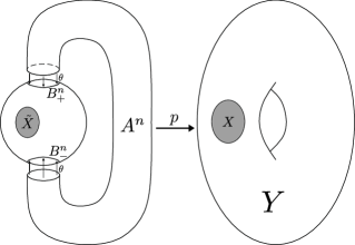
Due to Proposition 8 we may denote the manifold described there by . Let be a natural projection, be a locally flat ball, , and , . Since maps into homeomorphically, then is a locally flat ball (see Fig. 1). Due to Proposition 4, we immediately get the following statement.
Corollary 3.
Let be a locally flat ball. Then is homeomorphic to .
Lemma 1.
Let obtained from manifold by the surgery along . Then the following alternatives hold.
-
1.
If is disconnected, then where are connected components of ;
-
2.
if is connected and is orientable, then is homeomorphic to ;
-
3.
if is connected and is non-orientable then is homeomorphic either to or to .
Proof: If is disconnected, then the statement immediately follows from the definition of the connected sum. If is connected and is oriented, then the statement is proved in [31, Lemma 7]. So, we have to prove item 3. Suppose that is non-orientable and is connected.
By definition, there are disjoint locally flat balls such that is the result of gluing the annulus to by means of a homeomorphism . Let be a collar of . It follows from Proposition 4 that there exists a homeomorphism such that and . So, without loss of generality we may assume that (otherwise consider and instead of and ). Hence, belongs to the interior of a ball . A manifold is homeomorphic to the manifold described in Corollary 3. Let be a homeomorphism, and is an inclusion map. Then .
The following proposition is the generalisation of well-known facts in low dimension (see, for instance, [28, Lemma 3.17, Theorem 3.21]).
Proposition 9.
Let be a non-orientable closed manifold of dimension . Then
| (25) |
Proof: Recall that denotes either or . Set . Due to Theorem 2, . Hence, manifold can be considered as a result of the inverse surgery on . That means, that there are locally flat balls and a homeomorphism such that is homeomorphic to .
There are two possibilities: is either orientable or not, that depends only on the isotopy class of gluing map . It follows from Proposition 5 that there exists a homeomorphism such that is identity and is the orientation reversing. Set . Then and are non-isotopic and exhaust all possible isotopic classes of sphere homeomorphisms and all possible topological types of .
Determine a map by
| (26) |
If , then and . Hence, is a homeomorphism.
A manifold is said to be irreducible if any locally flat sphere bounds a ball . Any prime and non-irreducible three-dimensional manifold is homeomorphic to (see the proof in [28, Lemma 3.8]). We prove the following generalisation.
Proposition 10.
Any prime and non-irreducible manifold of dimension is homeomorphic to .
Proof: Suppose that is prime and non-irreducible. Then any locally flat -dimensional sphere in either bounds a ball in or does not separate . Let be a locally flat sphere that does not separate . Then a manifold obtained from by the surgery along is connected. Due to Lemma 1, . But is prime, hence, by Theorem 2, is homeomorphic to and is homeomorphic to .
2 Regular homeomorphisms
Let be a homeomorphism on a closed topological manifold with a metric . A point is said to be connected by an -chain of if there is a sequence of points and a sequence of integers such that , for . A number is called a length of the chain.
A point is chain recurrent for the homeomorphism if for any there are and -chain of length connecting to itself. The set of all chain recurrent points of is the chain recurrent set, and its connected components are chain components. It immediately follows form the definition, that the chain recurrent set is -invariant, hence, the following statement holds.
Proposition 11.
If the chain recurrent set of a homeomorphism is finite, than it consists of periodic points.
Suppose that is smooth, is a diffeomorphism, and is its periodic point of period . The point is called hyperbolic the differential of have no eigenvalues with absolute value equal to one. A number of eigenvalues of with absolute value greater that one is called a Morse index of . It follows from Grobman-Hartman Theorem (see [32, 33, 34])) and a classification of linear automorphisms of (see [35, Proposition 2.9])), that
there exists a neighbourhood of and a homeomorphism such that , where is a map defined by
| (27) |
and .
We call a periodic point of the homeomorphism topologically hyperbolic if the condition () holds. The number is called a Morse index of . If then is called a sink, if then is called a source, otherwise is called a saddle periodic point.
The map induces a splitting on invariant linear subspaces of dimensions , respectively, that are unstable and stable manifolds of a fixed point . A set is called a local unstable manifold, and a set is called an unstable manifold of the topologically hyperbolic periodic point . A local and global stable manifolds of the topologically hyperbolic periodic point is defined as the local and global unstable manifolds of with respect to . A connected component of the set is called an unstable stable separatrix of .
Due to [13, Statement 1],
| (28) |
A homeomorphism is called regular if its chain recurrent set is finite and topologically hyperbolic.
Morse-Smale diffeomorphism and gradient-like flows are important and motivating example of the regular dynamical systems. In general, trajectories of regular dynamical systems have more complex asymptotic behavior than ones for Morse-Smale systems since we omit a requirements of the transversality of the intersection of invariant manifolds. The following statements describe properties of regular homeomorphisms that they share with Morse-Smale diffeomorphisms. First two are proved in [13, Statement 2], [13, Theorem 1] for regular homeomorphism and in [36, Statement 1.2.5], [37, Theorem 2.3], for Morse-Smale diffeomorphism.
Following Smale, we determine a Smale relation on the set by the rule: if and only if .
Statement 11.
Let be a regular homeomorphism. Then
-
1.
for any points conditions imply ;
-
2.
there is no set of pairwise distinct points such that for any and .
Statement 12.
Suppose to be a regular homeomorphism. Then:
-
1.
;
-
2.
for any periodic point of Morse index the set is topological submanifolds of homeomorphic to ;
-
3.
for any .
Corollary 4.
Let be a topologically hyperbolic point of period , be a compact ball such that . Then there is a compact neighborhood of and a homeomorphism such that , , and projections along the fibers have the following properties:
-
1.
, ;
-
2.
, for any and .
Proof: Let be a neighborhood of and a homeomorphism satisfying condition . Remark that for any balls of dimension , respectively, containing the origin , a set has the properties described in the statement of the corollary, with the formal replacing with . Since , there is such that . Set . Due to Statement 12, Statement 11, is the submanifold of and . Hence we may choose in such a way that . Then the neighbourhood has the fibre structure with the required properties, and so does .
Set , . We say that if for some . Due to Statement 11, Smale relation can be extended to a total order relation on the set of periodic orbits of the regular homeomorphism as follows: if and only if either or .
Suppose that all periodic orbits consisting in are numbered with respect to the total order:
| (29) |
It follows from Statement 12 that contains at least one sink and one source periodic orbits. Then we may assume that first orbits in the row (29) are orbits of all sink periodic points from . Below we suppose that a set of saddle orbits of is non-empty, otherwise consists of exactly one sink and one source fixed points and is homeomorphic to the sphere as it shown in Proposition 12.
Set , . We call a maximal dimension of the unstable (stable) manifolds of the orbits the dimension of the set .
Recall that a set is called an attractor of if there exists a compact neighbourhood (a trapping neighbourhood) of such that and . A set is a repeller of if it is an attractor for .
The following proposition is similar to [38, Theorem 1.1], but is proved bypassing the smooth technique.
Theorem 3.
is an attractor with a trapping neighbourhood such that is a locally flat submanifold of . If , for any there exists a compact ball such that , and is embedded topologically transversely to .
Proof: We construct the trapping neighbourhood for using induction by .
Let , be a sink periodic point of period , and be a neighbourhood of and a homeomorphism satisfying the condition . Set . Since conjugates with and , then .
Let be a saddle periodic point. Then . Let be a compact ball such that . Due to Corollary 4, has a trivial microbundle in . Denote by a connected component of the set . Since for a any sink periodic point , there exists a single sink such that . There are two cases: 1) , 2) . In case 1) the set is connected and hence . Then there is a number such that for all , and, consequently, . According to Statement 6, there is an isotopy such that the ball is embedded topologically transversely to and .
In case 2), consists of two points that lays on different connected components of , and, possible, in stable manifolds of different sink periodic points . If belongs to different orbits, we choose the ball similar to case 1). If there exists a number such that , we choose a ball and set .
For any orbit , , choose a point and set . By construction, is the desired trapping neighbourhood for the set , .
Suppose that we built a trapping neighborhood for , . Let us construct the trapping neighbourhood for . There are two possibilities: 1) is the orbit of a source periodic point; 2) is the orbit of a saddle periodic point.
In case 1) set . Consider case 2). Let be a saddle periodic point with period and Morse index ; be a compact ball and its compact neighbourhood satisfying the conclusion of Corollary 4. By Corollary 4, there exists a homeomorphism such that . Set . Then . Remark that by Corollary 4 has a trivial microbundle in . Then so does .
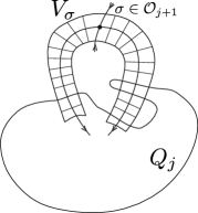
Since , and, moving to an iteration , if necessary, we may suppose that . Applying Statement 6 once more, we change near a neighbourhood of by an ambient isotopy so that is embedded topologically transversal to . We keep a notation for . Then is a submanifold of and . Moreover, is a boundary of and of . Then the set is bounded by a locally flat manifold (see Fig. 2).
It follows from Corollary 4 that .
Set and . By construction, is the desired trapping neighborhood for .
Corollary 5.
is a repeller of the regular homeomorphism . If then is connected.
To prove that is the repeller it is enough to apply the Theorem 3 to . The proof of the connectivity of for appropriate dimension of is literally the same as in [38, Theorem 1.1]. The idea of the proof is the following. Since , it does not divide . Then is connected and so does . Hence, is connected as an intersection of nested connected sets .
3 Proof of Theorem 1
3.1 Polar regular homeomorphisms
Recall that denotes a number of periodic points of the regular homeomorphism whose Morse index equals to . In this section we provide a proof of Theorem 1 for case . For smooth systems it follows from [38, Corollary 1.1] and [4, Theorem 1.3] (see also [26, Proposition 4.1]).
Proposition 12.
Let be a connected closed topological manifold of dimension and be a regular homeomorphism whose non-wandering set does not contain periodic points with Morse index equal to and . Then
-
1.
is polar;
-
2.
if has no heteroclinic intersections, then is homeomorphic to a sphere if and only if the set of saddle points of is empty;
-
3.
is simply connected.
Proof: Let us prove Item 1. Let be a union of all sink orbits of . Set . By the conditions, . Then due to Corollary 5, is connected, and, consequently, consists of a single point . Similar arguments for prove that the set of all source periodic orbits of is also consists of a single point . Hence, is polar.
The proof of Item 2 is completely similar to the proof of [4, Theorem 1.3]. We repeat here the main idea of it. If has no any saddle points, then its non-wandering set contains exactly one source and one sink and . Since is an open ball of dimension , is homeomorphic to the sphere . Suppose that is the sphere, the set of saddle periodic points of is non-empty and invariant manifolds of any saddle periodic point does not intersect invariant manifolds of other saddles. Then, due to Statement 12, . Hence, are spheres of dimension , respectively, that intersect each other at a single point . Then the intersection number of is different from zero. On the other hand, there is a sphere such that , and, consequently, the intersection number of equals zero. Since for , is homological to . Since the intersection number is a homological invariant, we obtain the contradiction that proves that the set of saddle periodic points of in this case is empty.
Let is prove Item 3. Suppose that the set of saddle periodic points of is not empty and consists of points of Morse indices . Then . Let be a loop representing a class . It follows from [39], that may be considered as a locally flat embedded circle. Let us show that can be moved by an ambient isotopy of to a loop . Since is homeomorphic to and, consequently, is simply connected, is homotopic to zero, and so would be , that meant is trivial.
We will construct the desired ambient isotopy moving sequentially outward unstable manifolds of all orbits preceding .
Due to Statement 6, there is an isotopy such that . Then there is a trapping neighbourhood of such that . Set . It follows from Theorem 3 that is compact and belongs to a union of compact balls laying in . Then, by Corollary 4, has a trivial normal microbundle in . Using Statement 6 once more, we construct an isotopy relative and such that is embedded topologically transversely to . Since , it means that . Hence, . Due to Theorem 3, is the attractor of with a trapping neighborhood . For a sufficiently large , we have . Repeating the arguments above, after a finite number of applying Statement 6 and Theorem 3, we get the desired isotopy.
3.2 A surgery along -dimensional separatrices
Previous section proves Theorem 1 for the case . If , we will use the surgery along locally flat sphere, introduced in Section 1.6. The following statements show that a closure of codimension one separatrix is a suitable sphere, more over, we may determine a regular homeomorphism from class on the resulting manifold .
Let be a saddle periodic point of a regular homeomorphism such that and does not contain heteroclinic points. It follows from Statement 12 that there is a unique sink periodic point such that and . Set .
Lemma 2.
is a locally flat -dimensional sphere.
Proof: Due to Statement 12, is a submanifold of homeomorphic to . Then is a sphere of dimension which is locally flat at all points except, possibly, . It follows from [40, Theorem 1] (see also [41, Corollary 3A.6]) that for the sphere cannot have one point of wildness (in fact, the set of points of wildness no less than uncountable). Then is locally flat at .
Corollary 6.
There is a neighbourhood of homeomorphic to and a number such that .
Proof: Due Proposition 2 and Statement 5, is a bi-collared sphere hence there is a topological embedding such that . Set .
Without loss of generality we suppose that all points of belong to the union (otherwise we take as the image of for sufficiently small ). Then for any point there is such that . Since is a homeomorphism, for any there is a neighbourhood such that for any . Since is compact, the set of neighbourhoods contains a finite subset , covering . Set . Then .
Remark 3.
Suppose that are fixed and (otherwise consider the diffeomorphism for an enough big ). It follows from Lemma 2 and Corollary 6, that the set consists of two -invariant connected components .
Proposition 13.
There is a homeomorphism such that
| (30) |
Proof: Set . Since belongs to an open annulus , it also can be embedded in . Due to Annulus theorem (see, for instance [26, Theorem 14.3] for references), is a union of two disjoint closed annuli . Suppose that . Then and for any there exists such that .
Let and be an arbitrary homeomorphism. Define a homeomorphism by . Then there exists a homeomorphism such that , (see [26, Proposition 14.2] for references). At last, define the desired homeomorphism by where and The homeomorphism can be constructed in similar way.
For points set if and denotes by a factor-space of . The natural projection induced on a structure of a topological manifold. Denote by a map that coincides with on and with on each connected component of . In fact, is homeomorphic to a closed manifold, obtained by gluing and two copies of by means of homeomorphisms . Hence we immediately got the following statement.
Lemma 3.
is homeomorphic to a closed manifold obtained from by surgery along
is a regular homeomorphism of and the number of periodic points of having Morse index is related to the number of periodic points of with Morse index as follows:
for all .
We will say that the pair is obtained from by surgery along .
Remark 4.
If is a smooth manifold, is Morse-Smale, and a pair is obtained from by the surgery along , then is smooth and is a Morse-Smale diffeomorphism.
3.3 End of the proof of Theorem 1
Let and . We may suppose that (in the opposite case we consider instead of ). Since we are interested only in topology of the manifold , we suppose without loss of generality that all periodic points of are fixed (that is 1-periodic, in the opposite case we may consider a homeomorphism for sufficiently large ).
Let us remark that if then similar to the proof of Proposition 12 we obtain that .
Since , there exists a saddle fixed point of Morse index which is the smallest with respect the Smale relation amount of all saddle fixed points. Then there is a source such that . Due to Lemma 6, the set is a locally flat sphere. Applying the surgery operation along , we obtain a pair of a closed topological manifold (may be disconnected) and a regular homeomorphism such that the restriction of on each connected component of belongs to class . If and , then has no saddle fixed points of indices and and, due to Proposition 12, have only one source. Then is connected and is polar. Due to Lemmas 3, 1, is homeomorphic to if is orientable, and to to if is non-orientable. Since is polar, it has only one sink. Hence, by Lemma 3 . Then and Theorem 1 is proved.
If , we do the surgery operation until we use up all the saddles of Morse index and after step we obtain a closed manifold and a regular homeomorphism . There are two possibilities: 1) ; 2) . In case 1) and after each surgery operation we obtain a connected closed manifold. Then is polar, is simply connected and is homeomorphic to if is orientable and to otherwise. Since is polar, it has only one sink. Hence, by Lemma 3 . Then and Theorem 1 is proved.
Consider case . Continue doing the surgery operation until we use up all the saddles of Morse index . Then after steps we obtain a closed manifold and a regular homeomorphism . Let us denote by the total number of connected components of . Due to Proposition 12, the restriction of on each connected component of is polar. Hence the non-wandering set of contains exactly sinks and sources. Since the total number of surgery operations is , using Proposition 3 one obtain that
| (31) |
At each surgery operation we have two possibilities: 1) the operation keeps the number of connected components obtained on the previous steps; 2) the operation increases by one the number of connected components obtained on the previous steps. Denote by the number of all operations that have been keeping the number of connected components. Then
| (32) |
References
- [1] Èl’sgol’ts, L. È An estimate for the number of singular points of a dynamical system defined on a manifold Matematicheskii Sbornik. Novaya Seriya, 1950, vol. 26, no. 2, pp 215–223.
- [2] Smale, S. Morse inequalities for a dynamical system, Bulletin of the American Mathematical Society, 1960, vol. 61. no. 1. pp. 43–49.
- [3] Bonatti, C., Grines, V., Medvedev, V. and Pecou, E. Three-dimensional manifolds admitting Morse-Smale diffeomorphisms without heteroclinic curves, Topology and Appl., 2002, vol. 117, pp. 335–344.
- [4] Grines, V. Z., Gurevich, E. Y. and Pochinka, O. V. Topological classification of Morse–Smale diffeomorphisms without heteroclinic intersections, Journal of Mathematical Sciences, 2015, vol. 208 (1), pp. 81-90.
- [5] Grines, V. Z. and Gurevich, E. Y. Morse Index of Saddle Equilibria of Gradient-Like Flows on Connected Sums of . Math Notes, 2022, vol. 111, pp. 624-–627.
- [6] Grines, V., Gurevich, E., Zhuzhoma, E. V. and Medvedev, V., On Topology of Manifolds Admitting a Gradient-Like Flow with a Prescribed Non-Wandering Set, Siberian Advances in Mathematics, 2019, vol. 29, no. 2, pp. 116-127.
- [7] Grines, V. Z. and Gurevich E. Y., Combinatorial invariant for gradient-like flows on the connected sum , Matematicheskiy sbornik, 2023, vol. 214, no. 5, pp. 97-127.
- [8] Grines, V. Z., Zhuzhoma, E. V. and Medvedev, V. S., On the structure of the ambient manifold for Morse-Smale systems without heteroclinic intersections, Trudy Matematicheskogo instituta im. V. A. Steklova RAN, 2017, vol. 297, pp. 201-210.
- [9] Grines, V. Z., Medvedev, V. S., Zhuzhoma, E. V., On the Topological Structure of Manifolds Supporting Axiom A Systems, Regular and Chaotic Dynamics, 2022, vol. 27, no. 6, pp. 613-628.
- [10] Gurevich, E., Sarayev I., Kirby diagram of polar flows on four-dimensional manifolds//Mathematical Notes, 2024, vol. 116, no. 6, pp. 40-57.
- [11] Pochinka, O. V., Osenkov E.M., The unique decomposition theorem for 3-manifolds, admitting Morse-Smale diffeomorphisms without heteroclinic curves, Moscow Math Journal (to appear)
- [12] Medvedev, T. V., Pochinka, O. V., Zinina, S. K., On existence of Morse energy function for topological flow, Advances in Mathematics., 2021, vol. 378, pp. 1-15.
- [13] Pochinka, O., Zinina, S., Construction of the Morse – Bott Energy Function for Regular Topological Flows, Regular and Chaotic Dynamics. 2021. Vol. 26. No. 4. P. 350-369.
- [14] Prasolov, V. V. Elements of homology theory, MCNMO, Moscow, 2006.
- [15] Mayer W. Über abstrakte Topologie, Monatsh. Math. und Physik, 1929, V. 36, P. 1—42, 219—258.
- [16] Vietoris L. Über die Homologiegruppen der Vereinigung zweier Komplexe, Monatshefte für Math. und Physik, 1930, V. 37, P. 159—162.
- [17] Hatcher, A., Algebraic topology, Cambridge University Press, 2002.
- [18] Brown, M. A., Locally Flat Imbeddings of Topological Manifold, Annals of Mathematics, Second Series, Mar., 1962, vol. 75, no. 2, pp. 331-341.
- [19] Gurevich, E. Y. and Saraev, I. A., On Morse-Smale Diffeomorphisms on Simply Connected Manifolds, Partial Differential Equations in Applied Mathematics, 2024, V. 11, https://doi.org/10.1016/j.padiff.2024.100759.
- [20] Milnor, J., "Microbundles. I". Topology. (1964). 3: 53–80.
- [21] Kirby, Robion C. and Siebenmann, Laurence C.. Foundational Essays on Topological Manifolds, Smoothings, and Triangulations. (AM-88), Volume 88, Princeton: Princeton University Press, 1977. https://doi.org/10.1515/9781400881505
- [22] F. Quinn, Topological transversality holds in all dimensions, Bull. Amer. Math. Soc. (N.S.) 18(2): 145-148.
- [23] Kervaire, M. A. and Milnor, J. W., Groups of Homotopy Spheres: I, The Annals of Mathematics, 2nd Ser., May, 1963, vol. 77, no. 3, pp. 504–537.
- [24] Rurk, K. and Sanderson, B., Introduction to piece wise linear topology, Moscow: Mir, 1974.
- [25] Brown, M. and Gluck, H. Stable Structures on Manifolds: III Applications, Annals of Mathematics, Second Series, Jan., 1964, vol. 79, no. 1, pp. 45-58.
- [26] Grines, V. Z., Gurevich, E. Y., Problems of topological classification of multidimensional Morse-Smale systems, Izhevsk: Izhevsk Institute for Computer Studies, 2022.
- [27] Kosniowski, C., A first course in algebraic topology, Cambridge University Press, 1980.
- [28] Hempel, J., 3-manifolds, Princeton, N.J. : Princeton University Press, 1976.
- [29] Gompf, R. E. and Stipsicz, A. I., 4-manifolds and Kirby Calculus, Graduate Studies in Mathematics, 1999.
- [30] Milnor, J., A Unique Decomposition Theorem for 3-Manifolds, American Journal of Mathematics, vol. 84, no. 1, 1962, pp. 1–7.
- [31] Medvedev, V. S and Umanskii, Ya. L., Decomposition of n-dimensional manifolds into simple manifolds, Izvestiya Vysshikh Uchebnykh Zavedenii. Matematika, no. 1, 1979, pp. 46-50.
- [32] Grobman, D. M. On the homeomorphism of systems of differential equations, Reports of the USSR Academy of Sciences, 1959, vol. 128, no. 5, pp. 880–881.
- [33] Grobman, D. M. Topological classification of neighborhoods of a singular point in -dimensional space, Mathematical Notes, 1962, vol. 56, no. 1, pp. 77–94.
- [34] Hartman, P. On the local linearization of differential equations, Proc. AMS., 1963, vol. 14, no. 4, pp. 568–573.
- [35] Palis, J. and De Melo, W. Geometric theory of dynamical systems. An introduction, Springer-Verlag, New York, Heidelberg, Berlin, 1982.
- [36] Grines, V. Z. and Pochinka, O. V., Introduction to the topological classification of cascades on manifolds of dimension two and three, “Regular and Chaotic Dynamics” Research Centre; Izhevsk Institute for Computer Studies, Moscow, Izhevsk, 2011.
- [37] Smale, S., Differentiable dynamical systems, Bull. Amer. Math. Soc., 1967, vol. 73 (6), pp. 747 – 817.
- [38] V. Z. Grines, E. V. Zhuzhoma, V. S. Medvedev, O. V. Pochinka, Global attractor and repeller of Morse-Smale diffeomorphisms, Proceedings of the Steklov Institute of Mathematics, 2010, Volume 271, Pages 103–124.
- [39] Dancis, J., General position maps for topological manifolds in the 2/3rds range. Transactions of the American Mathematical Society, vol. 216, 1976, pp. 249–266.
- [40] Kirby, R. C., On the Set of Non-Locally Flat Points of a Submanifold of Codimension One, Annals of Mathematics, Second Series, Sep., 1968, vol. 88, no. 2, pp. 281-290.
- [41] Daverman, J. R., Venema, G. A., Embeddings in Manifolds, Graduate Studies in Mathematics, vol. 10, 2009.