Measurement Induced Magic Resources

Abstract

Magic states and magic gates are crucial for achieving universal computation, but some important questions about how magic resources should be implemented to attain quantum advantage have remained unexplored, for instance, in the context of Measurement-based Quantum Computation (MQC) with only single-qubit measurements. This work bridges the gap between MQC and the resource theory of magic by introducing the concept of “invested” and “potential” magic resources. The former quantifies the magic cost associated with the MQC framework, serving both as a witness of magic resources and an upper bound for the realization of a desired unitary transformation. Potential magic resources represent the maximum achievable magic resource in a given graph structure defining the MQC. We utilize these concepts to analyze the magic resource requirements of the Quantum Fourier Transform (QFT) and provide a fresh perspective on the universality of MQC of different resource states, highlighting the crucial role of non-Pauli measurements for injecting magic. We demonstrate experimentally our theoretical predictions in a high-fidelity four-photon setup and demonstrate the efficiency of MQC in generating magic states, surpassing the limitations of conventional magic state injection methods. Our findings pave the way for future research exploring magic resource optimization and novel distillation schemes within the MQC framework, contributing to the advancement of fault-tolerant universal quantum computation.

1 Introduction

The ultimate goal of quantum computation is to achieve large-scale, fault-tolerant universal quantum computation [1]. To this end, one utilizes error correction codes to encode logical qubits and introduce sets of fault-tolerant universal gates [2, 3, 4]. Within this framework, T states/gates have been recognized as crucial resources, often referred to as magic states/gates, for achieving universal quantum computation. While Clifford gates alone are not universal, the combination of Clifford gates and T-states/gates provides the necessary ingredients for universal quantum computation, allowing for the generation of arbitrary quantum states with arbitrary precision. Additionally, T-states can be distilled from noisy encoded states, enhancing their practicality. These magic states/gates are fundamental resources towards fault-tolerant universal computation and can be quantified by the appropriate resource theory [5, 6, 7].

As depicted in Fig. 1(a), three key research areas are closely connected to magic resources and play a vital role in progressing towards fault-tolerant universal quantum computation: magic state distillation (MSD), magic state synthesis (MSS), and classical simulation complexity.

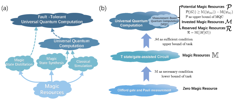
Figure 1: (a) Cartoon describing the relationship between magic resources and quantum computation tasks; (b) description of the three layers of quantum computation and their relationship with invested and potential magic resources.

MSD focuses on transforming noisy T-state encodings into higher-quality T-states suitable for practical applications [8, 4, 9]. Experimental progress has been made in this area [4, 9]. including demonstrations with 5-qubit [9] and 4-qubit codes [4]. Another application of the magic state is MSS, which leverages many T states/gates with Clifford gate and Pauli measurement to generate an arbitrary unitary or state [10]. Within the framework of quantum resource theory, the concept of magic resources provides fundamental lower bounds on the number of magic states/gates required for distillation and synthesis [11]. Understanding universal quantum computation also involves considering the complexity of simulating the same tasks on classical computers. The Gottesman-Knill theorem [12, 13, 14] moving beyond this first layer of computation, see Fig. 1(b)), injecting $k$ magic states (MSI), exponentially increases the difficulty of classical simulation as $2^{O(k)}\text{poly}(n)$. MSI involves preparing $n$ qubits in computational basis states and $k$ qubits in the T states, resulting in an $n+k$ qubit system. Simulating such a system with Clifford gates and Pauli measurements on a classical computer requires then a runtime scaling as $2^{O(k)}\text{poly}(n)$. From the perspective of classical simulation complexity, universal quantum computation is characterized by an exponential increase in resource requirements, which can be quantified by the magic resources present in the system.

Previous analyses of magic resources in the context of MSD, MSS, and classical simulation have primarily focused on the MSI framework. Recently, the issue of the magic resource cost of non-Pauli measurements has risen to attention [15, 16]. However, there is still a gap in our understanding of their role in the context of Measurement-based Quantum Computation (MQC) [17]. MQC is based on the preparation of a cluster state that is a stabilizer state associated with a graph - and therefore not possessing any magic resources - and achieves universality through consecutive single-qubit measurements, on graph stabilizer states, as evidenced by its proven universality [18]. This suggests that non-Pauli measurements within the MQC framework must generate magic resources, whereas the source of MQC’s universality has long been attributed to the versatile entanglement structure of graph states [18, 19]. This apparent incompleteness for the universality of MQC has not been fully recognized, and a general framework to incorporate both the entanglement structure and non-Pauli measurement to evaluate such universality is in demand.

This article consists of two parts: Theory and Experiment. In the first part, we establish the theory of invested magic resources and potential magic resources integrating the framework of MQC with magic resources, to provide a framework for understanding the source of MQC’s universality. Specifically, we show that invested magic resources provide an upper bound in the resources needed for the realization of a given quantum operation and provide sufficient magic resources for the Quantum Fourier Transform (QFT) [20]. In the second part, we experimentally verify the effectiveness of injecting magic with MQC in an optical platform, in which a four-photon cluster state is generated from two spontaneous parametric-down-conversion (SPDC) processes and post-selection [21], which is equivalent to the linear graph state and Box graph state [22]. The Linear graph is for single-qubit rotation and the Box state is for QFT for n=2. In the experiments, we find that MQC could effectively inject the magic resources in every step until the potential magic resources of the graph, and have advantages over MSI.

2 Theory

2.1 Background: Quantification of magic resources

Quantifying magic resources has been a challenging task in the field of quantum information. A fundamental approach involves measuring the extent to which a quantum state deviates from being a stabilizer state, which are states efficiently simulable on classical computers according to the Gottesman-Knill theorem. A reliable magic resource measure should satisfy three key properties: faithfulness, non-increasingness under the free operations of the theory (that is, Clifford operations), and (sub-)additivity. Faithfulness ensures that a state has zero magic if and only if it is a stabilizer state. Invariance under Clifford operations implies that applying Clifford gates, which are considered free operations in magic resource theories, does not alter the magic content of a state. Additivity dictates that the magic of a combined system is equal to the sum of the magic within its individual components. While measures like mana[23], robustness[24], thauma[25], and nullity[26] satisfy faithfulness and Clifford invariance, they lack the additivity property. Recent approaches based on stabilizer norm [24], stabilizer Rényi entropy[6, 7] and GKP codes[27] have successfully addressed this limitation, providing measures that fulfill all three desired criteria.

All these methods are deeply connected to the Pauli spectrum of a quantum state. For an n-qubit system, the Pauli group with quotient the overall phase, $\mathcal{P}_{n}$, consists of $\{I,X,Y,Z\}^{\otimes n}$. For any pure state $|\psi\rangle$, we can define the Pauli spectrum as the set of values ${\Xi_{P}}$, where $\Xi_{P}=d^{-1}\langle\psi|P|\psi\rangle^{2}$ for each Pauli operator $P\in\mathcal{P}_{n}$ and $d=2^{n}$ is the dimension of the Hilbert space. The Pauli spectrum satisfies the properties $\sum_{P}\Xi_{P}=1$ and $\Xi_{P}\geq 0$ for pure states, making it a probability distribution. Operationally, this is the probability of obtaining the state $|P\rangle:=I\otimes P|R\rangle$ when preparing $|\psi\rangle\otimes|\psi*\rangle$, where $|R\rangle:=d^{-1/2}\sum_{i}|ii\rangle$ is the maximally entangled state on two copies of the Hilbert space[37]. Using the Pauli spectrum, we can define the $\alpha$-Rényi entropy of the state for $\alpha\geq 0$:

$$\mathbb{M}_{\alpha}(|\psi\rangle)=(1-\alpha)^{-1}\log{\sum_{P}}\Xi_{P}^{\alpha}-\log d.$$ (1)

It has been proven that $\mathbb{M}_{\alpha}$ with $\alpha\geq 0$ serves as a reliable magic resource quantifier[6, 7], satisfying faithfulness ($M_{\alpha}(|\psi\rangle)=0$ if and only if $|\psi\rangle$ is a stabilizer state), Clifford invariance ($\mathbb{M}_{\alpha}(C|\psi\rangle)=\mathbb{M}_{\alpha}(|\psi\rangle)$ for any Clifford operation $C$), and additivity ($\mathbb{M}_{\alpha}(|\psi\rangle\otimes|\phi\rangle)=\mathbb{M}_{\alpha}(|\psi\rangle)+\mathbb{M}_{\alpha}(|\phi\rangle)$). Furthermore, $M_{\alpha}$ provides a lower bound for both the mana and nullity measures of magic and is also bounded by twice the robustness of magic. Notably, the case of $\alpha=1/2$ corresponds to the stabilizer-norm as $\log(\mathcal{D}(\psi))=1/2\mathbb{M}_{1/2}(|\psi\rangle)$ [38] and also the magic resource measure derived from GKP codes. Among all possible choices of $\alpha$, the 2-Rényi entropy ($\mathbb{M}_{2}$) stands out due to its generalizability to mixed states, which are crucial for describing realistic quantum systems, and its feasibility on the experiments [39]. Also, $\mathbb{M}_{2}$ is analytically tractable for a few important cases in many-qubit systems [40], and also can be numerically calculated by tensor network algorithms to large-scale [41, 42, 43].

For mixed states $\rho$, the Pauli spectrum no longer sums to 1 but instead reflects the purity of the state, with $\sum_{P}\Xi_{P}=\tr(\rho^{2})$. To address this, we consider a generalized Pauli spectrum given by $\Xi_{P}/\tr(\rho^{2})$. Consequently, the 2-Rényi entropy of the generalized Pauli spectrum takes the form:

$$\mathbb{M}_{2}(\rho)=-\log\sum_{P}\Xi_{P}^{2}-\log d-\mathbb{S}_{2}(\rho),$$ (2)

where $\mathbb{S}_{2}(\rho)=-\log\tr(\rho^{2})$ is the 2-Rényi entropy of the quantum state. In the resource theory for mixed states, there is also the partial trace, and although $\mathbb{M}_{2}(\rho)$ can sometimes increase under partial trace, numerical evidence shows that this is overwhelmingly rare, and therefore $\mathbb{M}_{2}(\rho)$ is a good proxy for this resource theory[6]. Another important comment is that the meaning of $\mathbb{M}_{2}(\rho)$ for mixed states is a bit different. In fact, there are states with $\mathbb{M}_{2}(\rho)=0$ from which no magic states are extractable. However, one important meaning they have is that they cannot be purified into states without magic[12, 44]. Moreover, this quantity is related to other to the cost of other protocols like learning and quantum verification[37, 45].

2.2 Review of MQC

This section delves into the role of non-Pauli measurements in MQC, also known as one-way computation due to the destructive nature of measurements on the quantum state, and their connection to the investment of magic resources.

The setup of MQC starts with a graph state $|G\rangle$, which is an entangled state of n qubits defined by a graph $G=(V,E)$ with n vertices and edges representing controlled-Z (CZ) gates. The graph state is obtained by applying CZ gates between qubits connected by edges in the graph, starting from an initial state of all qubits in $|+\rangle=(|0\rangle+|1\rangle)/\sqrt{2}$. Graph states are a special type of stabilizer state, meaning they possess a set of stabilizing operators that leave the state unchanged. For each qubit j in a graph state, there exists a stabilizer operator $K_{j}=X^{(j)}\prod_{i\in{N}(j)}Z^{(i)}$ involving the Pauli X operator on qubit j and Pauli Z operators on its neighboring qubits (${N}(j)$). Unlike the quantum circuit model, where quantum computations are achieved through a sequence of unitary gates and measurements, MQC relies on preparing a suitable graph state and performing a series of adaptive single-qubit measurements in the X-Y plane of the Bloch sphere. The final state of the computation is locally Pauli equivalent to the desired target state. Based on the stochastic outcomes of the measurements, additional Pauli corrections are applied to obtain the final result. This process can be summarized as the CME pattern, consisting of Entanglement (preparing the graph state), Measurement (adaptive single-qubit measurements), and Correction (Pauli corrections).

Such measurement calculus provides a framework for translating quantum circuits into equivalent MQC procedures[28, 29]. It relies on the fact that any unitary operation can be decomposed into a sequence of CZ gates and J gates, where the J gate is represented by the matrix $J(\alpha)=\frac{1}{\sqrt{2}}\begin{pmatrix}1&e^{i\alpha}\\ 1&-e^{i\alpha}\end{pmatrix}$. This decomposition process, known as J-decomposition, allows the expression of fundamental quantum gates like Hadamard($H=J(0)$), Pauli X($X=J(\pi)J(0)$), Pauli Z ($Z=J(0)J(\pi)$), Phase gate $S=J(0)J(\frac{\pi}{2})$ and rotations around the X and Z axes($R_{x}(\alpha)=J(\alpha)J(0)\ \&\ R_{z}(\alpha)=J(0)J(\alpha)$) using CZ and J gates. Each J gate in the decomposition corresponds to a small CME structure. For instance, the J gate with angle $\alpha$ can be implemented as:

$$J(\alpha):=X_{2}^{s_{1}}M_{1}^{-\alpha}E_{12},$$ (3)

where $E_{12}$ represents a CZ gate between qubits 1 and 2, $M_{1}^{-\alpha}$ denotes a measurement on the first qubit in the basis $(|0\rangle\pm e^{-i\alpha}|1\rangle)/\sqrt{2}$, $s_{1}$ is the measurement outcome, and $X_{2}^{s_{1}}$ is a Pauli X correction applied to the second qubit based on the measurement outcome. This equation illustrates how the action of $J(\alpha)$ on a state $|\psi\rangle$ can be achieved using an auxiliary qubit as the 2nd qubit initialized in the $|+\rangle$ state and an appropriate MQC procedure, as illustrated in Fig.2(a).

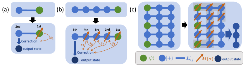
Figure 2: Demonstration of MQC. (a) shows how one rotation on one qubit is satisfied by MQC. The first is to build up the entanglement state $E_{12}|+\rangle|\psi\rangle$, then after the measurement on the input state and correction on the reserved qubit, we get $J(\alpha)|\psi\rangle$. (b) shows an arbitrary rotation for a single qubit. (c) shows how the 2D graph is used for MQC. The grey-shaped area for the transfer of the signals.

For more complex unitary operations, the measurement calculus utilizes swap relationships between operators to decompose them into sequences of J gates[29]. For example, an arbitrary single-qubit rotation $U$ can be expressed as $U=J(0)J(-\alpha)J(-\beta)J(-\gamma)$, which is equivalent to the Z-X-Z decomposition for SU(2), leading to an MQC implementation involving a linear graph of five qubits and four auxiliary qubits:

$$U|\psi\rangle =\underbrace{X_{5}^{s_{4}}M^{0}_{4}E_{45}}_{J(0)}\underbrace{X_{4}^{s_{3}}M^{\alpha}_{3}E_{43}}_{J(\alpha)}\underbrace{X_{3}^{s_{2}}M^{\beta}_{2}E_{32}}_{J(\beta)}\underbrace{X_{2}^{s_{1}}M^{\gamma}_{1}E_{21}}_{J(\gamma)}|\psi\rangle|+\rangle^{\otimes 4}$$ (4)

$$=\underbrace{X_{5}^{s_{2}+s_{4}}Z_{5}^{s_{1}+s_{3}}}_{{\text{correction}}}\underbrace{M_{4}^{0}M_{3}^{(-1)^{s_{2}}\alpha}M^{(-1)^{s_{1}}\beta}_{2}E_{1}^{\gamma}}_{{\text{measurement}}}\underbrace{E_{12345}|\psi\rangle|+\rangle^{\otimes 4}}_{{\text{entanglement}}}.$$

Fig.2(b) demonstrates this process and the transfer of signals of the measurement results. For the implementation of more complex unitary on multi-qubits states, we could use a 2-D graph to realize. see Fig.2(c).

By reordering the operators and grouping the entanglement operations and correction operations, we obtain a practical MQC plan where qubits are connected in a linear chain, and measurements are performed sequentially, adapting the measurement basis based on previous outcomes. This highlights the adaptive nature of measurements in MQC. Overall the CME pattern for the MQC could be summarized as:

$$U:=[C][M][E].$$ (5)

2.3 Invested Magic resources

From a resource-theoretic perspective, introducing auxiliary qubits in the $|+\rangle$ state, entangling them with CZ gates, and applying final Pauli corrections do not require any magic resources. As such, during the whole MQC procedure, the key source of magic resource investment lies in the non-Pauli measurements. These measurements lead to the generation of states with higher magic content, which is ultimately reflected in the final output state of the computation.

To quantify the magic resource investment associated with the adaptive measurements, we focus on the projected state of each measured qubit. Interestingly, the Pauli spectrum of these states remains the same regardless of the stochastic measurement outcomes. For the standard measurement $M^{\theta}$ onto $(|0\rangle\pm e^{i\theta}|1\rangle)/\sqrt{2}$, the Pauli spectrum is $\{\frac{1}{2},\frac{1}{2}\cos^{2}\theta,\frac{1}{2}\sin^{2}\theta,0\}$. Consequently, the magic resources required for the measurement, denoted as $\mathbb{M}_{\alpha}(\theta):=\mathbb{M}_{\alpha}((|0\rangle+e^{i\theta}|1\rangle)/\sqrt{2})$, are independent of the signal values. Specifically, for the 2-Rényi entropy, we have $\mathbb{M}_{2}(\theta)=-\log(\frac{1}{2}\cos^{4}\theta+\frac{1}{2}\sin^{4}\theta+\frac{1}{2})$.

Since each measurement setting $M^{\theta}$ in MQC corresponds to a J gate with angle $\theta$ in the J-decomposition of the target unitary $U$ in Eq.(5), we can define the total invested magic resources for implementing $U$ as:

$${\mathcal{M}}_{\alpha}(U):=\sum_{J(\theta)}\mathbb{M}_{\alpha}(\theta).$$ (6)

For example, the arbitrary rotation on the single qubits, $U=J(0)J(\alpha)J(\beta)J(\gamma)$. The corresponding magic resources on MQC is $\mathcal{M}_{\alpha}(U)=\mathbb{M}_{\alpha}(\alpha)+\mathbb{M}_{\alpha}(\beta)+\mathbb{M}_{\alpha}(\gamma)$.

This invested magic resource $\mathcal{M}_{\alpha}$ possesses the essential properties of a good magic resource measure. It exhibits faithfulness, meaning $\mathcal{M}_{\alpha}(C)=0$ if and only if $C$ is a Clifford gate. Additionally, $\mathcal{M}_{\alpha}$ is invariant under Clifford gates, meaning $\mathcal{M}_{\alpha}(CU)=\mathcal{M}_{\alpha}(U)$ for any Clifford gate $C$, as applying $C$ before or after $U$ does not change the magic resource cost. Finally, $\mathcal{M}_{\alpha}$ satisfies additivity, meaning $\mathcal{M}_{\alpha}(U\otimes V)=\mathcal{M}_{\alpha}(U)+\mathcal{M}_{\alpha}(V)$. The proof is left in Methods 5.1.

The invested magic resource measure $\mathcal{M}_{\alpha}$ offers a unique perspective compared to previous magic resource quantifiers. First, $\mathcal{M}_{\alpha}$ is naturally defined at the process level. Moreover, it is directly derived from the magic content of single-qubit states. Most importantly, while previous measures typically provide lower bounds on the magic resources required for a given task, $\mathcal{M}_{\alpha}$ serves to quantify a sufficient amount of resources for the task and also as a witness of employed magic resources. This means that if a quantum computation has an invested magic resource cost of $\mathcal{M}_{\alpha}$, there exists a concrete MQC implementation using that amount of magic resources.

2.4 Analysis on the Quantum Fourier Transform

In this section, we delve into the analysis of the Quantum Fourier Transform (QFT). The invested magic resource framework provides a useful tool for analyzing the complexity of QFT, offering an upper bound on the resources required for its implementation.

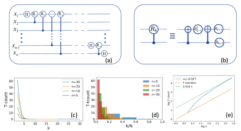
Figure 3: Demonstration of QFT and its invested magic resources. (a) The circuit model of QFT. (b) The J-decomposition of the control-rotation gate. (c) and (d) The invested magic resources distribution for different frequencies $k$. (e) The invested magic resources of QFT over qubit numbers. ‘T injection’ represents MSI with T-counts equals $n$.

QFT is a linear transformation that maps computational basis states $|x\rangle$ to the Fourier basis, $|x\rangle\xrightarrow[]{QFT}\sum_{k}\omega^{xk}|k\rangle$ with $\omega=\exp(i2\pi/2^{n})$ and $|k\rangle$ for Fourier bases. Fig. 3(a) shows the circuit implementation of QFT using Hadamard gates and controlled-rotation gates ($CR_{k}$) with $R_{k}=\text{diag}[1,\exp(i2\pi/2^{k})]$. The QFT circuit from the $j$-th qubit to the $n$-th qubits can be expressed iteratively as $\text{QFT}^{(j:n)}=\big{(}H^{(j)}\bigotimes_{i=j+1}^{n}C^{(i)}R_{i-j+1}^{(j)}\big{)}\text{QFT}^{(j+1:n)}$, where the superscripts indicate the qubit indices involved in each operation.

To analyze the magic resource cost of QFT, we utilize the J-decomposition technique, as shown in Fig. 3(b). Each $CR_{k}$ gate can be decomposed into two CNOT gates and three $R_{k+1}$ gates, with $R_{k+1}$ further decomposed as $J(0)J(2\pi/2^{k+1})$. Consequently, the invested magic resource cost of a $CR_{k}$ gate is given by $\mathcal{M}_{2}(CR_{k})=3\mathcal{M}_{2}(R_{k+1})=-3\log\left(\frac{1}{2}+\frac{1}{2}\cos^{4}\left(\frac{\pi}{2^{k}}\right)+\frac{1}{2}\sin^{4}\left(\frac{\pi}{2^{k}}\right)\right)$. For large values of $k$, this expression can be approximated as $\mathcal{M}_{2}(CR_{k})\approx-3\log\left(1+\left(\frac{\pi}{2^{k}}\right)^{4}\right)\approx\frac{3\pi^{4}}{2^{4k}}$, indicating that high-frequency components contribute minimally to the overall magic resource cost. Fig. 3(c) and (d) visualize the contribution of different frequencies to the invested magic resources of QFT. The plots reveal that most of the magic resources are concentrated in the low-frequency range, with a sharp decline in contribution as the frequency increases. This behavior remains consistent across different qubit numbers. Based on this observation, it is natural to consider a truncated QFT where only low-frequency components are included, potentially reducing the magic resource cost without significant loss of accuracy.

The full QFT for $n$ qubits requires $(n+k-1)$ instances of $CR_{k}$ gates for each frequency $k$. By summing the magic resource contributions from all frequencies up to a cut-off value $m$ and approximating the contributions from higher frequencies, we obtain:

$$\mathcal{M}_{2}(\text{QFT}) =\sum_{k=2}^{n}(n+k-1)\mathcal{M}_{2}(CR_{k})$$ (7)

$$\approx\sum_{k=2}^{m}(n+k-1)\mathcal{M}_{2}(CR_{k})+\sum_{k=m}^{n}(n+k-1)\frac{3\pi^{4}}{2^{4k}}$$

$$\approx 3.4619n-5.3388.$$

There are a total of $3(m^{2}+2mn-2n-m)/2$ J gates for the truncated QFT and $9(n^{2}-n)/2$ J gates for the complete QFT. For a sufficiently large cut-off frequency $m$, the second term becomes negligible, and the invested magic resource cost of QFT scales linearly with the number of qubits: $\mathcal{M}_{2}(\text{QFT})\approx 3.46n-5.34$ (in units of T-count). This result, visualized in Fig. 3(e), suggests that QFT can be implemented with a relatively modest amount of magic resources compared to the full complexity of the circuit.

Previous analyses of classical simulation algorithms for QFT circuits have suggested a complexity of $O(n\log n)$ T gates [46]. However, the invested magic resource framework provides an upper bound on the required resources, indicating that $O(n)$ T gates might be sufficient. This aligns with the observation that truncated QFT, which primarily involves low-frequency components, can provide a good approximation of the full QFT with reduced complexity [32]. Our analysis further supports this notion by demonstrating that the majority of magic resources are concentrated in the lower frequencies, and the cut-off frequency for an accurate approximation is independent of the qubit number. Since magic resources are directly related to classical simulation complexity, we can conclude that truncated QFT exhibits similar complexity to the full QFT while requiring significantly fewer resources.

2.5 Potential Magic resources

While designing specific graphs for targeted tasks is one approach to MQC, a more general strategy involves preparing versatile graph states capable of performing arbitrary quantum computations. These versatile graphs are often referred to as universal resources for MQC [18, 19, 17]. However, it’s important to recognize that not all invested magic resources effectively contribute to the magic content of the final state. This limitation arises from the inherent maximum potential of magic resources that a particular graph type can hold, which we term potential magic resources $\mathcal{P}$.

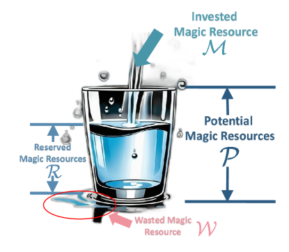
Figure 4: Cartoon showing the relationship between invested magic resources ($\mathcal{M}$), potential magic resources ($\mathcal{P}$), and reserved magic resources ($\mathcal{R}$).

Previous analyses of universal resources for MQC have attributed their versatility to the rich entanglement structures they possess. A measure called “entanglement width” ($E_{wt}$) has been introduced to quantify this potential for entanglement [19, 18]. If a state $|\psi\rangle$ can be transformed into another state $|\phi\rangle$ using local operations and classical communication (LOCC), denoted as ${|\psi\rangle}\geq_{LOCC}|\phi\rangle$, then the entanglement width satisfies $E_{wt}(|\psi\rangle)\geq E_{wt}(|\phi\rangle)$. Furthermore, a family of states qualifies as a universal resource if their entanglement width is unbounded. As previously mentioned, such an understanding for the university is incomplete because it undervalues the effects of the non-Pauli measurement. Therefore, it needs to be connected with the entanglement structure with the magic resources.

Analogously, we can define reserved magic resources $\mathcal{R}$ and potential magic resources $\mathcal{P}$ in the following way. Given a preparation obtained by a set of measurements $[M]$ on a graph state $|G\rangle$, its reserved magic resource is defined as

$$\mathcal{R}([M]|G\rangle):=\mathbb{M}_{2}([M]|G\rangle)$$ (8)

i.e. the magic resources of the remaining state after the measurement. We then define the potential magic resources as the maximum magic resources brought by the entanglement structure $[E]$. For example, the potential magic resource $\mathcal{P}(|G\rangle)$ of a graph state $|G\rangle$ as the maximum achievable magic content under any set of measurements $[M]$ on an arbitrary number of qubits:

$$\mathcal{P}(|G\rangle):=\max_{[M]}\mathbb{M}_{2}([M]|G\rangle).$$ (9)

The above definition is motivated by the fact that the entanglement structure is fundamental to determining how much magic can be hosted in a certain state. Indeed. product states are far from the average states (which are very entangled) in terms of their stabilizer entropy [6]. In Eq.9, one implies as input as reference state the pure input state $|+\rangle$ on every qubit. Additionally, MQC allows for a general quantum input, $[E]|\psi\rangle=|G\rangle*|\psi\rangle$, with $*$ as link product [33, 34] between the graph and the input state and $|G\rangle$ as a graph with some links vacant. Therefore, the maximum increment of the magic resources brought by the entanglement structure with the input $|\psi\rangle$ shows

$$\mathcal{P}(G;|\psi\rangle)=\max_{[M]}\mathbb{M}_{2}([M]|G\rangle*|\psi\rangle)-\mathbb{M}_{2}(|\psi\rangle)$$ (10)

Note that Eq. (10) is a general version of Eq. (9). Therefore, if MQC can produce a state $|\phi\rangle$ or its Clifford equivalents from the input state $|\psi\rangle$ with a graph $|G\rangle$, denoted as $|G\rangle*|\psi\rangle\geq_{\text{MQC}}|\phi\rangle$, the potential magic resources must satisfy $\mathcal{P}(|G\rangle;|\psi\rangle)\geq\mathbb{M}_{2}(|\phi\rangle)-\mathbb{M}_{2}(|\psi\rangle)$. Consequently, a family of graph states can serve as universal resources only if their potential magic resources are unbounded.

A key application of this concept lies in demonstrating the limitations of linear graphs and GHZ states as universal resources, regardless of their size. From the perspective of potential magic resources, we can show that:

$$\mathcal{P}(|\text{Linear}\rangle)=1T,\quad\mathcal{P}(|\text{GHZ}\rangle)=1T.$$ (11)

The fact that linear and GHZ states have limited potential magic resources implies that the computational power they offer through magic resources is constant and does not scale with the system size. This finding provides a novel perspective on the concept of universality in MQC, highlighting the importance of potential magic resources as a measure of the capability of different graph structures.

Fig. 4 visually summarizes the relationship between the invested magic resources ($\mathcal{M}$), potential magic resources ($\mathcal{P}$), and reserved magic resources ($\mathcal{R}$) using the analogy of pouring water into a glass. The invested magic resources represent the total amount of magic available (the water being poured), while the potential magic resources correspond to the capacity of the glass. The reserved magic resources represent the amount of water that successfully fills the glass, and any excess water that spills over signifies wasted magic resources, which could be defined as $\mathcal{W}=\mathcal{M}-\mathcal{P}$.

3 Experimental Results

The invested magic resources, $\mathcal{M}_{2}$, enable us to quantify the magic resources injected into the network in MQC. The magic resources of the remaining state after each step of measurement, $\mathcal{R}$, represent the reserved magic resources. By introducing these concepts, we can indicate the invested and reserved magic resources step by step in the MQC process.

We focus on two typical processes: single-qubit rotation and QFT. We demonstrate how the magic responds to single-qubit measurements in 1-D and 2-D graph states. The 1D graph state is a linear state, while the 2D graph state is a BOX state. Both originate from the 4-qubits cluster state, $|\text{cluster}\rangle=(|0000\rangle+|0011\rangle+|1100\rangle-|1111\rangle)/2$ [22]. For the specific setup see Methods 5.3. The experimental estimation of reserved magic resources derives from the few-shot randomized measurements [35, 36], with more explanations on the few-shot estimator left in Methods 5.4.

3.1 Arbitrary rotation from 1-D linear state

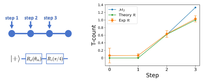
Figure 5: Experimental generation of the $|T\rangle$ state using a 1D graph in three steps. The left side visually depicts the process, starting from an initial cluster state (Step 0) and progressing through steps of measurement subject to a standard MQC pattern. The angles of $M^{\theta}$ are ${0,\theta_{m},\pi/4}$ for steps 1, 2, and 3, respectively. The plot on the right displays the total invested magic resources $\mathcal{M}_{2}$ and the reserved magic resource $\mathcal{R}$ at each step. Error bars are estimated using the bootstrap method.

Our experiment utilizes a linear graph and MQC to generate the $|T\rangle$ state. The process can be mathematically expressed with a cluster state in the CME pattern as:

$$|T\rangle=X^{s_{2}}Z^{s_{1}+s_{3}}[M_{3}^{\pi/4}]^{s_{2}}[M_{2}^{\theta_{m}}]^{s_{1}}[M_{1}^{0}]|\text{cluster}\rangle.$$ (12)

Here, $s_{i}$ represents the binary measurement outcome on the $i_{\text{th}}$ measurement. Although the measurement outcomes on each qubit are random and influence subsequent measurement settings and corrections, our previous analysis established that they do not affect the overall magic resources within the system. Therefore, we average the final magic resources over all possible single-qubit measurement outcomes to obtain an estimation.

The comparison between the invested and reserved magic resources in the process is illustrated in Fig.5. The reserved magic resources are 0, 0.62T, and 1T, with accumulated invested magic resources of 0T, 0.62T, and 1.33T, respectively. It can be seen that the invested and reserved magic are equal during the first two steps of the process. However, for the third step, a waste of magic resources $\mathcal{W}=0.33\mathrm{T}$ is inevitable because the invested magic resources exceed the potential magic resources for a linear graph $\mathcal{P}=1\mathrm{T}$.

3.2 QFT from 2-D Box state

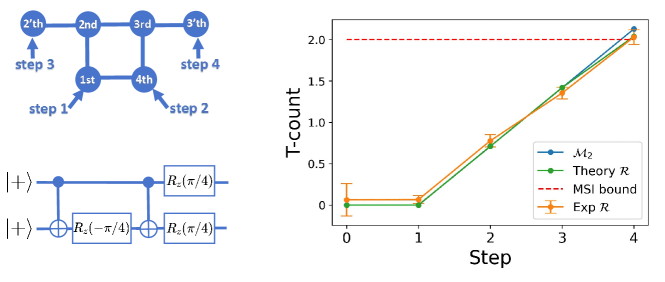
Figure 6: Experimental realization of QFT using a 2D graph. The left side of the figure depicts the 2D graph structure employed for implementing the QFT circuit of $n=2$ (left bottom) and indicates the order of measurements performed on the qubits (steps 1 to 4). The generation of $|\text{CS}\rangle$ from MQC requires at least 6 qubits, as the figure shows. Step 3 on the 2’th qubit and step 4 on the 3’th qubit are equivalent to the local rotation for the physical qubits 2nd and 3rd qubit. In this way, we can achieve the generation of $|\text{CS}\rangle$ from a BOX state with merely four qubits, denoted as 1st, 2nd, 3rd, and 4th. According to Eq.(13), implementing $M_{1}^{0}$, $M_{4}^{(\pi/8,0)}$, $\hat{T}_{2}$, and $\hat{T}_{3}$ corresponds to the steps 1 to 4, in which $M_{4}^{(\pi/8,0)}$ is for non-standard measurement $M^{(\phi,\theta)}$, projection onto $\{\cos\phi|0\rangle\pm e^{-i\theta}\sin\phi|1\rangle\}$, and $\hat{T}$ is T-gate $\hat{T}=\text{diag}[1,e^{i\pi/4}]$. See Methods 5.5 for details. The right side of the figure presents the evolution of invested and reserved magic resources throughout the QFT process. The blue line represents the invested magic, quantified by $\mathbb{M}_{2}$, while the green line depicts the theoretical expectation for the reserved magic resources ($\mathcal{R}$). Step 0 and step 1 are the same as Fig. 5 and the estimated $\mathcal{R}$ and error bars are calculated from an average of 80 incidents per measurement basis. The red dashed line indicates the upper bound for MSI, which is 2T in this case as only two qubits are retained in the final state. The orange dots represent the experimentally measured values of $\mathbb{M}_{2}$, demonstrating good agreement with the theoretical predictions.

We demonstrate the generation of QFT of $n=2$ in MQC. QFT requires controlled-rotation gates with arbitrary angles, denoted as $CR_{k}=\text{diag}[1,1,1,e^{i2\pi/2^{k}}]$, which is challenging to demonstrate in a traditional circuit model. Here for $n=2$, it shows $CR_{2}=\text{diag}[1,1,1,i]$, also known as $CS$ gate. The power of QFT is evident in the resulting QFT state, defined as $|\text{QFT}_{n}\rangle=\text{QFT}_{n}|+\rangle|0\rangle^{\otimes(n-1)}$, which possesses a nullity of $\nu(|\text{QFT}_{n})\rangle=n-2$ [26]. For $n=2$, the QFT state $|\text{QFT}_{2}\rangle=|\text{CS}\rangle=(|00\rangle+|01\rangle+|10\rangle+i|11\rangle)/2$, representing the state with maximum magic content for a two-qubit system, can be generated from the MQC, see Fig. 6. The resulting CME pattern for generating the $|\text{CS}\rangle$ state is given by:

$$|\text{CS}\rangle=X_{3}Z_{3}^{s_{4}}Z_{2}^{s_{1}}\hat{T}_{3}\hat{T}_{2}[M_{4}^{(\pi/8,0)}][M_{1}^{0}]|\text{cluster}\rangle.$$ (13)

The invested magic resources increase by approximately $0.71T$ with each step of the process. Consequently, the accumulated invested magic resources for steps 1 to 4 are $0\mathrm{T}$, $0.71\mathrm{T}$, $1.42\mathrm{T}$, and $2.13\mathrm{T}$, respectively. The corresponding reserved magic resources are $0T$, $0.71\mathrm{T}$, $1.41\mathrm{T}$, and $2.03\mathrm{T}$. The inevitable wasted magic resources are merely $\mathcal{W}=0.1T$. In the experiments, we obtain $0.066\pm 0.024\mathrm{T},0.777\pm 0.036\mathrm{T},1.354\pm 0.036\mathrm{T},2.030\pm 0.045\mathrm{T}$. Notably, almost all the invested magic resources are successfully injected into the system except for the last step, where $\mathcal{M}=2.13T$ is greater than potential $\mathcal{P}=2.03\mathrm{T}$, bringing the inevitable waste of $\mathcal{W}=0.1\mathrm{T}$.

Furthermore, MQC offers a significant advantage over the conventional MSI approach. With MSI, the maximum achievable magic resources for an n-qubit state are limited to nT. However, MQC, by strategically employing auxiliary qubits and sequential measurements, can generate states with magic content exceeding the qubit number. For example, the $|\text{CS}\rangle$ state, while comprising only 2 qubits, contains 2.03T of magic, and the Hoggar state, a 3-qubit state, holds 3.6T of magic. Both of these states can be efficiently generated using MQC, demonstrating its space-saving potential for quantum processors.

4 Discussion

This paper introduces the novel concepts of invested and potential magic resources to provide a deeper understanding of the role of magic in MQC. Invested magic resources quantify the magic resource cost associated with MQC procedures, serving both as a witness and upper bound for the magic resources needed for quantum tasks. Being an upper bound, this also quantifies a sufficient amount of magic resources for the task. Potential magic resources, on the other hand, represent the maximum achievable magic content within different graph structures associated with MQC.

In this paper, these notions are developed at the theory level and demonstrated at the experimental level. We analyzed the upper bound of magic resources required for QFT, improving the resource estimate from $O(n\log n)$ to $O(n)$. This analysis also sheds light on the potential for resource-efficient implementations of QFT using truncated versions that primarily involve low-frequency components. Furthermore, our work provides a fresh perspective on the universality of MQC resources. We demonstrate that entanglement alone is insufficient for universality and that non-Pauli measurements play a crucial role in injecting the necessary magic resources, provided the underlying graph structure has sufficient potential to hold them.

To validate our theoretical framework, we conducted high-fidelity experiments using a four-photon setup to meticulously track the evolution of invested and reserved magic resources throughout MQC processes. We introduced a more efficient method for measuring magic resources experimentally and applied it to investigate single-qubit rotations with a 1D linear graph and QFT implementation with a 2D box graph. Our results confirm the theoretical predictions, showing that the reserved magic resources increase with each non-Pauli measurement step.

Furthermore, our findings suggest that MQC offers a more efficient approach for generating magic states compared to the conventional MSI method. MQC exhibits superior space efficiency, requiring fewer qubits to achieve the same level of magic resource, and can even surpass the limitations imposed by the MSI bound.

Given the essential role of magic states in fault-tolerant universal quantum computation, MQC emerges as a promising framework for magic state generation and utilization. Our work paves the way for future research exploring more efficient methods for magic state injection through non-Pauli measurements and developing novel distillation schemes tailored for MQC. Additionally, it raises intriguing open questions regarding the relationship between invested and reserved magic resources, as well as the connection between potential magic resources and entanglement measures.

5 Methods

5.1 Proof of Invested Magic resources as a good measure

For an arbitrary unitary $U$, there exists a possible MQC process to realize it. We calculated the magic resources needed in the MQC to guarantee the necessary conditions to realize $U$. This depends on the J-decomposition of the unitary with $\mathcal{M}(U)=\sum_{J(\theta)}\mathbb{M}_{\alpha}[M(\theta)]$. We will prove that it satisfies faithfulness, invariance with Clifford gates, and additivity.

First, it exhibits faithfulness, meaning $\mathcal{M}_{\alpha}(C)=0$ if and only if $C$ is a Clifford gate. This follows from the fact that Clifford gates can be decomposed into CZ gates, Hadamard gates (equivalent to $J(0)$), and phase gates (equivalent to $J(0)J(\frac{\pi}{2})$), all of which have zero magic cost according to $\mathcal{M}_{\alpha}$. Conversely, if $\mathcal{M}_{\alpha}(U)=0$, then the unitary $U$ can only involve gates generated by $\{CZ,J(0),J(\frac{\pi}{2}),J(\pi)\}$, which correspond to Clifford operations.

Additionally, invariance under Clifford gates means $\mathcal{M}_{\alpha}(CU)=\mathcal{M}_{\alpha}(U)$ for any Clifford gate $C$, as applying $C$ before or after $U$ does not change the magic resource cost. Similar to faithfulness, Clifford gates can be decomposed by the Hadamard gate, the phase gate, and the CZ gate, and they can all be implemented with no invested magic resources.

Finally, additivity means $\mathcal{M}_{\alpha}(U\otimes V)=\mathcal{M}_{\alpha}(U)+\mathcal{M}_{\alpha}(V)$. $U$ and $V$ represent two independent MQC procedures. Suppose a greater graph with $|G\rangle=|G_{U}\rangle*|G_{V}\rangle$. The half graph $|G_{U}\rangle$ realizes $U$, and the other half $|G_{V}\rangle$ realizes $V$. Thus, the additivity is always satisfied.

5.2 Analysis on Potential Magic resources

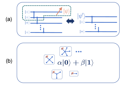
Figure 7: Computation process of the Potential Magic Resources for Linear and GHZ state

In this section, we prove that the potential magic resources of linear graph states and GHZ states are both $1\mathrm{T}$, as described by Eq. (9).

The proof for linear graph states is illustrated in Fig. 7(a). A linear graph with $n$ qubits, denoted as $|L_{n}\rangle$, is defined by $|L_{n}\rangle=\bigotimes_{j=1}^{n-1}E_{j+1,j}|+\rangle^{\otimes n}$, where $E_{j+1,j}$ is the CZ gate between the $(j+1)_{th}$ and $j_{th}$ qubits. Suppose we perform a projection measurement with the state $|\psi\rangle=\alpha|0\rangle+\beta|1\rangle$, the resulting state after the projection is given by $\tr_{1}\big{[}|\psi\rangle\langle\psi|\otimes|L_{n}\rangle\big{]}=E_{12}|\psi^{\prime}\rangle|L_{n-2}\rangle$ with normalization, where $|\psi^{\prime}\rangle=\alpha^{*}|+\rangle+\beta^{*}|-\rangle$. As shown in Fig. 7(a), we can move the remaining CZ gates that do not involve the measured qubit to a position after the measurement. Thus, the measurement on the first qubit is equivalent to state preparation on $|\psi^{\prime}\rangle$. This process can be repeated for each subsequent qubit measurement. Suppose we have $m$ qubits to be measured with measurements $M_{1}$ to $M_{m}$. Then, we have:

$$\mathbb{M}_{2}\Big{[}M_{m}\dots M_{2}M_{1}|L_{n}\rangle|\Big{]}= \mathbb{M}_{2}\Big{[}M_{m}\dots M_{2}E_{12}|\psi^{\prime}\rangle|L_{n-2}\rangle\Big{]}$$ (14)

$$= \mathbb{M}_{2}\Big{[}E_{12}|\psi^{\prime\prime}\rangle|L_{n-m-1}\rangle]$$

$$= \mathbb{M}_{2}[|\psi^{\prime\prime}\rangle]\leq 1\mathrm{T},$$

where $|\psi^{\prime\prime}\rangle$ is some 1-qubit state related to the measurement settings and results. According to the definition of potential magic resources, we have $\mathcal{P}(|L_{n}\rangle)=1\mathrm{T}$.

For GHZ states, as shown in Fig. 7(b), an $n$-qubit GHZ state can be written as $|\text{GHZ}_{n}\rangle=\frac{1}{\sqrt{2}}(|\mathbf{0}_{n}\rangle+|\mathbf{1}_{n}\rangle)$, which is locally Clifford equivalent to ”star-like” graphs with a central qubit connected to $n-1$ outer qubits. Consider a projection state $|\psi\rangle=\alpha|0\rangle+\beta|1\rangle$. After projection, the remaining state becomes $\alpha^{*}|\mathbf{0}_{n-1}\rangle+\beta^{*}|\mathbf{1}_{n-1}\rangle$. This process can be repeated multiple times. After consecutive single-qubit measurements, the GHZ state is always equivalent to $\alpha|\mathbf{0}_{n-1}\rangle+\beta|\mathbf{1}_{n-1}\rangle$ with some $\alpha$ and $\beta$. Thus, we have:

$$\mathbb{M}_{2}\Big{[}M_{m}\dots M_{2}M_{1}|\text{GHZ}_{n}\rangle\Big{]}= \mathbb{M}_{2}\Big{[}\alpha|\mathbf{0}_{n-m}\rangle+\beta|\mathbf{1}_{n-m}\rangle\Big{]}$$ (15)

$$= \mathbb{M}_{2}\Big{[}CX|0\rangle\otimes(\alpha|\mathbf{0}_{n-m-1}\rangle+\beta|\mathbf{1}_{n-m-1}\rangle)\Big{]}$$

$$= \mathbb{M}_{2}\Big{[}\alpha|0\rangle+\beta|1\rangle\Big{]}\leq 1\mathrm{T},$$

where $CX$ is the CNOT gate between $|0\rangle$ and the remaining $\alpha|\mathbf{0}_{n-m-1}\rangle+\beta|\mathbf{1}_{n-m-1}\rangle$. This process can be repeated until the final single qubit. According to the definition of potential magic resources, we have $\mathcal{P}(|\text{GHZ}_{n}\rangle)=1\mathrm{T}$.

Thus, we have proven that the potential magic resources for both linear graph states and GHZ states are $1\mathrm{T}$.

5.3 Experimental Setup

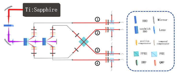
Figure 8: Scheme of the Experimental Setup. A femtosecond laser centered at 780 nm (produced by a Ti:Sapphire laser) pumps a $\beta$-barium borate (BBO) crystal, generating violet light centered at 390 nm. This violet beam then pumps two separate BBO crystals in a ”sandwich-like” configuration to create polarization-entangled photon pairs via type-II spontaneous parametric down-conversion (SPDC). Each sandwich BBO consists of a 2mm-thick BBO crystal, a zero-order half-wave plate, and a 1mm-thick BBO crystal. Here, the two extraordinary photons (e-photons) from both sources are directed to meet at a partial polarization beam splitter (PPBS) with $t_{H}=1$ and $t_{V}=1/3$. Hong-Ou-Mandel (HOM) interference occurs at the interface of PPBS. By post-selecting events where exactly one photon is detected in each output path, a cluster state is generated. This state is then measured using local single-qubit projective measurements, which involve a quarter-wave plate (QWP), a half-wave plate (HWP), and a polarization beam splitter (PBS).

cluster state can be generated using an optical CNOT gate acting on two maximally entangled states. However, the success rate and fidelity of this method are not satisfactory. Therefore, we adopted the setup described in [21] to produce a high-quality cluster state from two non-maximally entangled states and a partial-polarization beam splitter (PPBS). The setup to produce the cluster state is shown in Fig. 8. A femtosecond violet light sequentially pumps two sandwich-like $\beta$-barium borate (BBO) crystals. Each BBO sandwich comprises a 2mm-thick BBO crystal, a zero-order half-wave plate, and a 1mm-thick BBO crystal. The BBO crystals are beam-like cut [47] to enhance brightness. The 2mm-thick BBO triples the brightness of the SPDC photons compared to the 1mm-thick BBO. This, along with position and temporal compensation and a half-wave plate (HWP) on one side, enables the generation of non-maximally polarization-entangled photons in the state $(|HH\rangle+\sqrt{3}|VV\rangle)/\sqrt{2}$. By adjusting the delay lines between the two sources, the two extraordinary photons (e-photons) from both sources are directed to meet at a PPBS. This PPBS has transmission coefficients of $t_{H}=1$ for horizontally polarized light and $t_{V}=1/3$ for vertically polarized light, and it introduces an $i$ phase shift for the reflected photon. When two vertically polarized photons meet at the PPBS interface, Hong-Ou-Mandel interference occurs. Consequently, a 4-photon polarization cluster state emerges after the PPBS, described by $|\text{cluster}\rangle=(|HHHH\rangle+|HHVV\rangle+|VVHH\rangle-|VVVV\rangle)/\sqrt{2}$, with a success rate of $1/4$. Following the definition of the cluster state, the qubit labels are assigned as shown in Fig. 8. Photons from the first source represent qubits 1 and 2, while photons from the second source represent qubits 3 and 4. To optimize performance, 2nm filters are placed on the branches of qubits 2 and 3, and 3nm filters are placed on qubits 1 and 4, to eliminate the influence of frequency correlations. Further setup details can be found in [21].

Fig. 9 shows the performance of the cluster state. A cluster state can be defined by 16 stabilizer bases, $B_{i}$, which can be calculated from 9 bases in experiments. To avoid multi-photon errors, the violet beam power was set to 40mW. By collecting 200 incidents per basis, we obtained the results shown in Fig. 9. The overall fidelity is $\langle\text{cluster}|\psi|\text{cluster}\rangle=\sum_{i=1}^{16}\langle B_{i}\rangle=0.923\pm 0.001$. The error is calculated using Bootstrap.

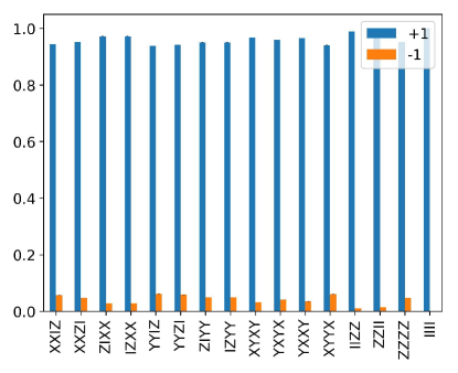
Figure 9: Stabilizer of the cluster state. Experimental results on testing the 16 stabilizers of the cluster state, which are calculated from 9 bases in the experiments: ZZZZ, ZZXX, XXZZ, YYZZ, ZZYY, XYXY, YXYX, XYYX, YXXY. “+1” and “-1” are for the eigenvalues of the stabilizer, and the bar is for the percentage per eigenstate in experiments.

5.4 Estimating Reserved Magic Resources $\mathcal{R}$ from Randomized Measurement

One experimental task involves quantifying the remaining magic resources $\mathcal{R}$ within a quantum state after undergoing MQC measurement. Since $\mathcal{R}(\ket{G})=\mathbb{M}_{2}([M]|G\rangle)$, estimating $\mathcal{R}$ involves estimating $\mathbb{M}_{2}$ in the experiments. As shown in Ref. [39], $\mathbb{M}_{2}$ can be effectively estimated on IBM’s 5-qubit and 7-qubit quantum processors.

Following established methods, we experimentally determined $\mathbb{M}_{2}$ using randomized measurements. $\mathbb{M}_{2}$ is calculated as $-\log\sum_{P}\Xi_{P}^{2}-\log d$, where $\Xi_{P}=\langle P\rangle^{2}/d$ and $P$ represents elements within the Pauli group $\mathcal{P}(n)$ excluding the identity and global phase factors. Interestingly, $\mathbb{M}_{2}$ can also be understood as a fourth-order property of a quantum state, expressible as $\mathbb{M}_{2}=-\text{tr}(Q\psi^{\otimes 4})-\log d$ for pure states $\psi$. Here, $Q=d^{-2}\sum_{P}P^{\otimes 4}$ involves the fourth tensor power of Pauli operators. While the Clifford group does not form a 4-design necessary for direct estimation of this fourth-order property, we can still leverage randomized Clifford measurements to estimate $\mathbb{M}_{2}$ using the following expression with every 4-incidents pairs:

$$\mathbb{M}_{2}(\psi)=-\log\mathbb{E}_{\vec{s}}\left[(-2)^{-s_{1}\oplus s_{2}\oplus s_{3}\oplus s_{4}}\mathbb{E}_{C\in\mathcal{C}l(n)}\prod_{i=1}^{4}\mathrm{Pr}(s_{i}|C)\right]-\log d,$$ (16)

where $s_{i}$ is an n-bit string as outcomes of the experiments and $\oplus$ denotes bit-wise binary addition, $s_{1}\oplus s_{2}\oplus s_{3}\oplus s_{4}=\sum_{i}s_{1}^{i}\land s_{2}^{i}\land s_{3}^{i}\land s_{4}^{i}$.

For mixed states $\rho$, the Pauli spectrum $\Xi_{P}$ requires normalization since $\sum_{P}\Xi_{P}=\text{tr}(\rho^{2})$. We introduce $\tilde{\Xi}_{P}=\Xi_{P}/\text{tr}(\rho^{2})$ and modify $\mathbb{M}_{2}$ to incorporate the 2-Rényi entropy of the state, $\mathbb{S}_{2}(\rho)=-\log\text{tr}(\rho^{2})$. We have $\mathbb{M}_{2}=-\text{tr}(Q\rho^{\otimes 4})-\log d-\mathbb{S}_{2}(\rho)$. Both $\mathbb{M}_{2}$ and $\mathbb{S}_{2}(\rho)$ can be estimated from the same randomized Clifford measurements, exploiting the fact that the Clifford group forms a 3-design [48, 49]. $\mathbb{S}_{2}(\rho)=-\log\sum_{(s_{1},s_{2})}(-2)^{s_{1}\oplus s_{2}}\mathbb{E}_{C\in\mathcal{C}l(n)}\prod_{i=1}^{2}\mathrm{Pr}(s_{i}|C)-\log d$ [50, 51, 52]. The resulting expression for mixed states becomes:

$$\mathbb{M}_{2}(\rho)= -\log\mathbb{E}_{\vec{s}}\left[(-2)^{-s_{1}\oplus s_{2}\oplus s_{3}\oplus s_{4}}\mathbb{E}_{C\in\mathcal{C}l(n)}\prod_{i=1}^{4}\mathrm{Pr}(s_{i}|C)\right]$$ (17)

$$-\log\mathbb{E}_{\vec{s}}\left[(-2)^{s_{1}\oplus s_{2}}\mathbb{E}_{C\in\mathcal{C}l(n)}\prod_{i=1}^{2}\mathrm{Pr}(s_{i}|C)\right].$$

Indeed, since the fourth-order operator $Q$ and the second-order Swap operator can both be written into the product of single-qubit ones, the previous estimators can be evaluated by from the random single-qubit Clifford unitary, say the Pauli measurement [39]. Moreover, employing the few-shot treatment [35, 36], we arrive at a concise few-shot estimator of $\mathbb{M}_{2}$ used in the experiment:

$$\mathbb{M}_{2}(\rho)=-\log\mathbb{E}_{P}\mathbb{E}_{\vec{s}}\left[(-2)^{-s_{1}\oplus s_{2}\oplus s_{3}\oplus s_{4}}\right]-\log\mathbb{E}_{P}\mathbb{E}_{\vec{s}}\left[(-2)^{-s_{1}\oplus s_{2}}\right],$$ (18)

where $P$ represents Pauli measurement setting chosen from the set $\{X,Y,Z\}^{\otimes n}$ with equal possibility of $1/3^{n}$. The estimation process is as follows: (1) randomly select a Pauli measurement $P$ from $\{X,Y,Z\}^{\otimes n}$, (2) collect $N_{M}$ outcomes, each an n-bit string, (3) for each 4-string pair in $N_{M}$ outcomes, calculate $(-2)^{-s_{1}\oplus s_{2}\oplus s_{3}\oplus s_{4}}$ and for each 2-string pair in $N_{M}$ outcomes, calculate $(-2)^{-s_{1}\oplus s_{2}}$, and (4) calculate the means of the calculated values for all Pauli measurements using Eq.(18).

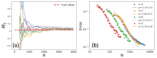
Figure 10: The experimental demonstration of measuring $\mathbb{M}_{2}$ with randomized measurement. (a) Estimation of $\mathbb{M}_{2}$ of cluster state over the number of collected photons. (b) Scaling of estimation $\mathbb{M}_{2}$ over the number of collected photons for $n=1$ to $n=4$ linear cluster states in a log-log diagram. Dots represent the experimental results with uncertainty calculated from Bootstrap over the total photon number used. The dashed line represents the linear regression results.

The experimental implementation and results of the randomized measurement (RM) method for estimating $\mathbb{M}_{2}$ are presented in Fig. 10. This figure showcases an example of using RM to quantify the magic within a 4-qubit cluster state (a specific entangled state) and illustrates the performance. A graphic processing unit (GPU), Nvidia GeForce RTX 3070, is used to accelerate the post-processing. Estimating $\mathbb{M}_{2}$ involves calculating the value of $(-2)^{s_{1}\oplus s_{2}\oplus s_{3}\oplus s_{4}}$ for every possible combination of four measurement outcomes within each measurement setting. With $N$ measurement outcomes, the number of such 4-incident-pairs $N^{\prime}=\binom{N}{4}$ scales as $N^{4}$. Consequently, for a small number of measurement outcomes, the estimation error of $\mathbb{M}_{2}$ exhibits a $1/N^{2}$ dependence. However, as $N$ increases further, the uncertainty reduction slows and approaches $1/\sqrt{N}$ scaling. This phenomenon has been previously noted in similar studies in estimating entanglement [53]. In the experiments, the linear regression in Fig. 10(b) shows that $\log\text{Err}=-1.7\log N+b$, validating the calculation. The experimental data aligns with this theoretical understanding. A linear regression analysis on the log-log diagram in Fig. 10(b) observes a slope of $-1.7$. This result validates the expected scaling behavior and confirms the effectiveness of the RM method for estimating $\mathbb{M}_{2}$.

5.5 Arbitrary Measurement-Induced Magic Resources

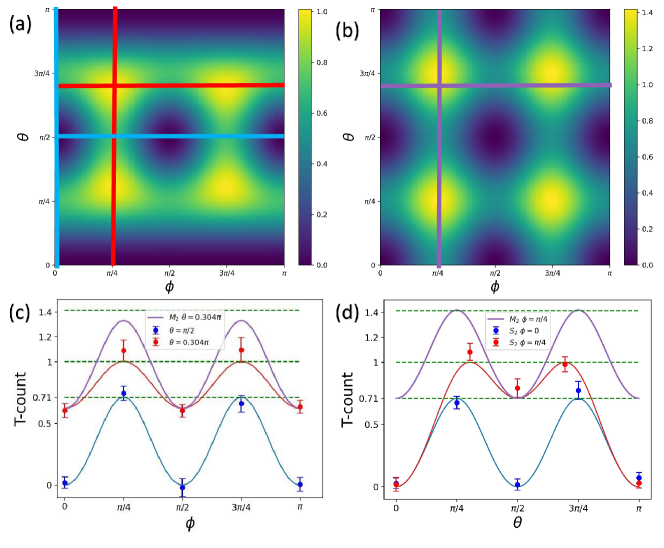
Figure 11: Magic resources under arbitrary single-qubit measurements. This figure explores the relationship between invested and reserved magic resources when performing arbitrary single-qubit measurements of the form $|\psi\rangle=\cos\theta|0\rangle+\sin\theta e^{i\phi}|1\rangle$ on a maximally entangled state. (a) illustrates the reserved magic resources after the measurement, while (b) depicts the invested magic resources following the standard MQC pattern, calculated as $\mathbb{M}_{2}(|\psi\rangle)=\mathbb{M}_{2}(M^{\theta})+\mathbb{M}_{2}(M^{\phi})$. (c) and (d) focus on specific cases with fixed angles. (c) shows the invested magic resources for fixed values of $\theta$, comparing the arbitrary measurement case (red line for $\theta=\theta_{m}$) with the standard MQC pattern (grey line for $\theta=\theta_{m}$) and a measurement with $\theta=\pi/2$ (blue line). Similarly, (d) presents the invested magic resources for fixed values of $\phi$, comparing the arbitrary measurement case (red line for $\phi=\pi/4$) with the standard MQC pattern (grey line for $\phi=\pi/4$) and measurement with $\phi=0$ (blue line). Dots in (c) and (d) represent experimental results with error bars from Bootstrap with 80 incidents per Pauli basis, which demonstrate good agreement with the theoretical predictions. Importantly, the invested magic resources for the arbitrary form measurements always match the reserved magic resources, as indicated by the alignment of the blue and red lines in subfigures (a) and (c)-(d) with the corresponding lines in (b).

Measurement-based quantum computation (MQC) with linear graphs allows for arbitrary single-qubit rotations, enabling versatile quantum operations. However, the standard MQC approach, which employs measurements of the form $(|0\rangle+e^{i\phi}|1\rangle)/\sqrt{2}$, can lead to unnecessary consumption of magic resources, as demonstrated in Fig. 5. To address this issue, we explore the use of arbitrary single-qubit measurements to minimize magic resource waste. Consider an arbitrary single-qubit measurement described by the basis states $|\psi_{\pm}\rangle=\cos\theta|0\rangle\pm\sin\theta e^{i\phi}|1\rangle$. We can show that $|\psi_{+}\rangle$ can be obtained by a maximally entangled state ($E_{12}|+\rangle^{\otimes 2}$) followed by a specific single-qubit measurement $M_{1}^{(\theta,\phi)}$ and a Pauli Z correction ($Z_{2}^{s}$) depending on the measurement outcome: $|\psi_{+}\rangle=Z_{2}^{s}M_{1}^{(\theta,\phi)}E_{12}|+\rangle^{\otimes 2}$. In this case, the invested magic resources are equal to the $\mathbb{M}_{2}$ of the outcome state $|\psi\rangle$.

Compared to the standard MQC approach, where the invested magic resources are given by $\mathbb{M}_{2}(M^{(\theta,\phi)})\leq\mathbb{M}_{2}(M^{\theta})+\mathbb{M}_{2}(M^{\phi})$, the arbitrary measurement scheme offers a significant advantage. The standard MQC approach generally requires more magic resources than the amount preserved in the final state $\mathbb{M}_{2}(|\psi_{\pm}\rangle)$, leading to unnecessary waste.

This analysis reveals that any MQC computation on a linear graph can be efficiently implemented using just a single auxiliary qubit and an appropriately chosen arbitrary measurement, effectively eliminating magic resource waste. Fig. 11 illustrates the impact of arbitrary measurements on magic resource consumption. The grey line, representing the invested magic resources for the standard MQC approach, is noticeably higher than the red line and dots, which depict the invested and reserved magic resources, respectively, for the arbitrary measurement case. The blue line and dots represent a similar comparison for a different set of measurement angles, further demonstrating the advantage of arbitrary measurements in conserving magic resources.

Declarations

This work was supported by the Innovation Program for Quantum Science and Technology (Nos. 2021ZD0301200, 2021ZD0301400, 2021ZD0302000), National Natural Science Foundation of China (Grant Nos. 12122410, 12350006, 12205048, 11821404), Anhui Initiative in Quantum Information Technologies (AHY060300), the Fundamental Research Funds for the Central Universities (Grant No. WK2030000038, WK2470000034). AH acknowledges support from PNRR MUR project PE0000023-NQSTI and PNRR MUR project CN $00000013$ -ICSC.

References

- \bibcommenthead
- Campbell et al. [2017] Campbell, E.T., Terhal, B.M., Vuillot, C.: Roads towards fault-tolerant universal quantum computation. Nature 549(7671), 172–179 (2017)
- Postler et al. [2022] Postler, L., Heuen, S., Pogorelov, I., Rispler, M., Feldker, T., Meth, M., Marciniak, C.D., Stricker, R., Ringbauer, M., Blatt, R., et al.: Demonstration of fault-tolerant universal quantum gate operations. Nature 605(7911), 675–680 (2022)
- AI [2023] AI, G.Q.: Suppressing quantum errors by scaling a surface code logical qubit. Nature 614(7949), 676–681 (2023)
- Gupta et al. [2024] Gupta, R.S., Sundaresan, N., Alexander, T., Wood, C.J., Merkel, S.T., Healy, M.B., Hillenbrand, M., Jochym-O’Connor, T., Wootton, J.R., Yoder, T.J., et al.: Encoding a magic state with beyond break-even fidelity. Nature 625(7994), 259–263 (2024)
- Veitch et al. [2014] Veitch, V., Mousavian, S.H., Gottesman, D., Emerson, J.: The resource theory of stabilizer quantum computation. New Journal of Physics 16(1), 013009 (2014)
- Leone et al. [2022] Leone, L., Oliviero, S.F., Hamma, A.: Stabilizer rényi entropy. Physical Review Letters 128(5), 050402 (2022)
- Leone and Bittel [2024] Leone, L., Bittel, L.: Stabilizer entropies are monotones for magic-state resource theory. arXiv preprint arXiv:2404.11652 (2024)
- Bravyi and Kitaev [2005] Bravyi, S., Kitaev, A.: Universal quantum computation with ideal clifford gates and noisy ancillas. Physical Review A 71(2), 022316 (2005)
- Souza et al. [2011] Souza, A.M., Zhang, J., Ryan, C.A., Laflamme, R.: Experimental magic state distillation for fault-tolerant quantum computing. Nature communications 2(1), 169 (2011)
- Knill [2005] Knill, E.: Quantum computing with realistically noisy devices. Nature 434(7029), 39–44 (2005)
- Regula and Takagi [2021] Regula, B., Takagi, R.: Fundamental limitations on distillation of quantum channel resources. Nature Communications 12(1), 4411 (2021)
- Aaronson and Gottesman [2004] Aaronson, S., Gottesman, D.: Improved simulation of stabilizer circuits. Physical Review A 70(5), 052328 (2004)
- Bravyi and Gosset [2016] Bravyi, S., Gosset, D.: Improved classical simulation of quantum circuits dominated by clifford gates. Physical review letters 116(25), 250501 (2016)
- Bravyi et al. [2016] Bravyi, S., Smith, G., Smolin, J.A.: Trading classical and quantum computational resources. Physical Review X 6(2), 021043 (2016)
- Oliviero et al. [2021] Oliviero, S.F., Leone, L., Hamma, A.: Transitions in entanglement complexity in random quantum circuits by measurements. Physics Letters A 418, 127721 (2021)
- Niroula et al. [2023] Niroula, P., White, C.D., Wang, Q., Johri, S., Zhu, D., Monroe, C., Noel, C., Gullans, M.J.: Phase transition in magic with random quantum circuits. arXiv preprint arXiv:2304.10481 (2023)
- Briegel et al. [2009] Briegel, H.J., Browne, D.E., Dür, W., Raussendorf, R., Nest, M.: Measurement-based quantum computation. Nature Physics 5(1), 19–26 (2009)
- Van den Nest et al. [2007] Nest, M., Dür, W., Miyake, A., Briegel, H.J.: Fundamentals of universality in one-way quantum computation. New Journal of Physics 9(6), 204 (2007)
- Van den Nest et al. [2006] Nest, M., Miyake, A., Dür, W., Briegel, H.J.: Universal resources for measurement-based quantum computation. Physical review letters 97(15), 150504 (2006)
- Nielsen and Chuang [2001] Nielsen, M.A., Chuang, I.L.: Quantum Computation and Quantum Information vol. 2. Cambridge university press Cambridge, ??? (2001)
- Zhang et al. [2016] Zhang, C., Huang, Y.-F., Liu, B.-H., Li, C.-F., Guo, G.-C.: Experimental generation of a high-fidelity four-photon linear cluster state. Physical Review A 93(6), 062329 (2016)
- Walther et al. [2005] Walther, P., Resch, K.J., Rudolph, T., Schenck, E., Weinfurter, H., Vedral, V., Aspelmeyer, M., Zeilinger, A.: Experimental one-way quantum computing. Nature 434(7030), 169–176 (2005)
- Veitch et al. [2014] Veitch, V., Mousavian, S.H., Gottesman, D., Emerson, J.: The resource theory of stabilizer quantum computation. New Journal of Physics 16(1), 013009 (2014)
- Howard and Campbell [2017] Howard, M., Campbell, E.: Application of a resource theory for magic states to fault-tolerant quantum computing. Physical review letters 118(9), 090501 (2017)
- Wang et al. [2020] Wang, X., Wilde, M.M., Su, Y.: Efficiently computable bounds for magic state distillation. Physical review letters 124(9), 090505 (2020)
- Beverland et al. [2020] Beverland, M., Campbell, E., Howard, M., Kliuchnikov, V.: Lower bounds on the non-clifford resources for quantum computations. Quantum Science and Technology 5(3), 035009 (2020)
- Hahn et al. [2022] Hahn, O., Ferraro, A., Hultquist, L., Ferrini, G., García-Álvarez, L.: Quantifying qubit magic resource with gottesman-kitaev-preskill encoding. Physical Review Letters 128(21), 210502 (2022)
- Danos et al. [2005] Danos, V., Kashefi, E., Panangaden, P.: Parsimonious and robust realizations of unitary maps in the one-way model. Physical Review A 72(6), 064301 (2005)
- Danos et al. [2007] Danos, V., Kashefi, E., Panangaden, P.: The measurement calculus. Journal of the ACM (JACM) 54(2), 8 (2007)
- Shor [1994] Shor, P.W.: Algorithms for quantum computation: discrete logarithms and factoring. In: Proceedings 35th Annual Symposium on Foundations of Computer Science, pp. 124–134 (1994). Ieee
- Kitaev [1995] Kitaev, A.Y.: Quantum measurements and the abelian stabilizer problem. arXiv preprint quant-ph/9511026 (1995)
- Coppersmith [2002] Coppersmith, D.: An approximate fourier transform useful in quantum factoring. arXiv preprint quant-ph/0201067 (2002)
- Chiribella et al. [2008] Chiribella, G., D’Ariano, G.M., Perinotti, P.: Quantum circuit architecture. Physical review letters 101(6), 060401 (2008)
- Chiribella et al. [2009] Chiribella, G., D’Ariano, G.M., Perinotti, P.: Theoretical framework for quantum networks. Physical Review A 80(2), 022339 (2009)
- Zhou et al. [2020] Zhou, Y., Zeng, P., Liu, Z.: Single-copies estimation of entanglement negativity. Phys. Rev. Lett. 125, 200502 (2020) https://doi.org/10.1103/PhysRevLett.125.200502
- Li et al. [2024] Li, G.-C., Chen, L., Zhang, S.-Q., Hong, X.-S., Zhou, Y., Chen, G., Li, C.-F., Guo, G.-C.: Directly estimating mixed-state entanglement with bell measurement assistance. arXiv preprint arXiv:2405.20696 (2024)
- Leone et al. [2024] Leone, L., Oliviero, S.F., Hamma, A.: Learning t-doped stabilizer states. Quantum 8, 1361 (2024)
- Campbell [2011] Campbell, E.T.: Catalysis and activation of magic states in fault-tolerant architectures. Physical Review A 83(3), 032317 (2011)
- Oliviero et al. [2022] Oliviero, S.F., Leone, L., Hamma, A., Lloyd, S.: Measuring magic on a quantum processor. npj Quantum Information 8(1), 148 (2022)
- Chen et al. [2023] Chen, J., Yan, Y., Zhou, Y.: Magic of quantum hypergraph states. arXiv preprint arXiv:2308.01886 (2023) https://doi.org/10.48550/arXiv.2308.01886
- Haug and Piroli [2023] Haug, T., Piroli, L.: Quantifying nonstabilizerness of matrix product states. Phys. Rev. B 107, 035148 (2023) https://doi.org/10.1103/PhysRevB.107.035148
- Lami and Collura [2023] Lami, G., Collura, M.: Nonstabilizerness via perfect pauli sampling of matrix product states. Phys. Rev. Lett. 131, 180401 (2023) https://doi.org/10.1103/PhysRevLett.131.180401
- Tirrito et al. [2024] Tirrito, E., Tarabunga, P.S., Lami, G., Chanda, T., Leone, L., Oliviero, S.F., Dalmonte, M., Collura, M., Hamma, A.: Quantifying nonstabilizerness through entanglement spectrum flatness. Physical Review A 109(4), 040401 (2024)
- Cao et al. [2024] Cao, C., Cheng, G., Hamma, A., Leone, L., Munizzi, W., Oliviero, S.F.: Gravitational back-reaction is the holographic dual of magic. arXiv preprint arXiv:2403.07056 (2024)
- Leone et al. [2023] Leone, L., Oliviero, S.F., Hamma, A.: Nonstabilizerness determining the hardness of direct fidelity estimation. Physical Review A 107(2), 022429 (2023)
- Nam et al. [2020] Nam, Y., Su, Y., Maslov, D.: Approximate quantum fourier transform with o (n log (n)) t gates. NPJ Quantum Information 6(1), 26 (2020)
- Kurtsiefer et al. [2001] Kurtsiefer, C., Oberparleiter, M., Weinfurter, H.: Generation of correlated photon pairs in type-ii parametric down conversion—revisited. Journal of Modern Optics 48(13), 1997–2007 (2001)
- Zhu [2017] Zhu, H.: Multiqubit clifford groups are unitary 3-designs. Physical Review A 96(6), 062336 (2017)
- Li et al. [2023] Li, G.-C., Yin, Z.-Q., Zhang, W.-H., Chen, L., Yin, P., Peng, X.-X., Hong, X.-S., Chen, G., Li, C.-F., Guo, G.-C.: Experimental full calibration of quantum devices in a semi-device-independent way. Optica 10(12), 1723–1728 (2023)
- Brydges et al. [2019] Brydges, T., Elben, A., Jurcevic, P., Vermersch, B., Maier, C., Lanyon, B.P., Zoller, P., Blatt, R., Roos, C.F.: Probing rényi entanglement entropy via randomized measurements. Science 364(6437), 260–263 (2019)
- Elben et al. [2019] Elben, A., Vermersch, B., Roos, C.F., Zoller, P.: Statistical correlations between locally randomized measurements: A toolbox for probing entanglement in many-body quantum states. Physical Review A 99(5), 052323 (2019)
- Elben et al. [2023] Elben, A., Flammia, S.T., Huang, H.-Y., Kueng, R., Preskill, J., Vermersch, B., Zoller, P.: The randomized measurement toolbox. Nature Reviews Physics 5(1), 9–24 (2023)
- Elben et al. [2020] Elben, A., Kueng, R., Huang, H.-Y.R., Bijnen, R., Kokail, C., Dalmonte, M., Calabrese, P., Kraus, B., Preskill, J., Zoller, P., et al.: Mixed-state entanglement from local randomized measurements. Physical Review Letters 125(20), 200501 (2020)