RVI-SAC:
Average Reward Off-Policy Deep Reinforcement Learning

Abstract

In this paper, we propose an off-policy deep reinforcement learning (DRL) method utilizing the average reward criterion. While most existing DRL methods employ the discounted reward criterion, this can potentially lead to a discrepancy between the training objective and performance metrics in continuing tasks, making the average reward criterion a recommended alternative. We introduce RVI-SAC, an extension of the state-of-the-art off-policy DRL method, Soft Actor-Critic (SAC) (Haarnoja et al., 2018a, b), to the average reward criterion. Our proposal consists of (1) Critic updates based on RVI Q-learning (Abounadi et al., 2001), (2) Actor updates introduced by the average reward soft policy improvement theorem, and (3) automatic adjustment of Reset Cost enabling the average reward reinforcement learning to be applied to tasks with termination. We apply our method to the Gymnasium’s Mujoco tasks, a subset of locomotion tasks, and demonstrate that RVI-SAC shows competitive performance compared to existing methods.

1 Introduction

Model-free reinforcement learning aims to acquire optimal policies through interaction with the environment. Particularly, Deep Reinforcement Learning (DRL), which approximates functions such as policy or value using Neural Networks, has seen rapid development in recent years. This advancement has enabled solving tasks with high-dimensional continuous action spaces, such as those in OpenAI Gym’s Mujoco tasks (Todorov et al., 2012). In the realm of DRL methods applicable to tasks with high-dimensional continuous action spaces, methods such as TRPO (Schulman et al., 2015), PPO (Schulman et al., 2017), DDPG (Silver et al., 2014; Lillicrap et al., 2019), TD3 (Fujimoto et al., 2018), and SAC (Haarnoja et al., 2018a, b) are well-known. These methods utilize the discounted reward criterion, which is applicable to a variety of MDP-formulated tasks (Puterman, 1994). In particular, for continuing tasks where there is no natural breakpoint in episodes, such as in robot locomotion (Todorov et al., 2012) or Access Control Queuing Tasks(Sutton & Barto, 2018), where the interaction between an agent and an environment can continue indefinitely, the discount rate plays a role in keeping the infinite horizon return bounded. However, discounting introduces an undesirable effect in continuing tasks by prioritizing rewards closer to the current time over those in the future. An approach to mitigate this effect is to bring the discount rate closer to 1, but it is commonly known that a large discount rate can lead to instability and slower convergence(Fujimoto et al., 2018; Dewanto & Gallagher, 2021).

In recent years, the average reward criterion has begun to gain attention as an alternative to the discounted reward criterion. Reinforcement learning using the average reward criterion aims to maximize the time average of the infinite horizon return in continuing tasks. In continuing tasks, the average reward criterion is considered more natural than the discounted reward criterion. Even within the realm of DRL with continuous action space, although few, there have been proposals for methods that utilize the average reward criterion. Notably, ATRPO (Zhang & Ross, 2021) and APO (Ma et al., 2021), which are extensions of the state-of-the-art on-policy DRL methods, TRPO and PPO, to the average reward criterion, have been reported to demonstrate performance on par with or superior to methods using the discounted reward criterion in Mujoco tasks (Todorov et al., 2012).

Research combining the average reward criterion with off-policy methods, generally known for their higher sample efficiency than on-policy approaches, remains limited. There are several theoretical and tabular approaches to off-policy methods using the average reward criterion, including R-learning (Schwartz, 1993; Singh, 1994), RVI Q-learning (Abounadi et al., 2001), Differential Q-learning (Wan et al., 2020), and CSV Q-learning (Yang et al., 2016). However, to our knowledge, the only off-policy DRL method with continuous action space that employs the average reward criterion is ARO-DDPG (Saxena et al., 2023) which optimize determinisitic policy. In DRL research using discount rate, Maximum Entropy Reinforcement Learning, which optimizes stochastic policies for entropy-augmented objectives, is known to improve sample efficiency significantly. Off-policy DRL methods with continuous action space that have adopted this concept (Mnih et al., 2016; Haarnoja et al., 2017, 2018a, 2018b; Abdolmaleki et al., 2018) have achieved success. However, to the best of our knowledge, there are no existing DRL methods using the average reward criterion as powerful and sample-efficient as Soft-Actor Critic.

Our goal is to propose RVI-SAC, an off-policy Actor-Critic DRL method that employs the concept of Maximum Entropy Reinforcement Learning under the average reward criterion. In our proposed method, we use a new Q-Network update method based on RVI Q-learning to update the Critic. Unlike Differential Q-learning, which was the basis for ARO-DDPG, RVI Q-learning can uniquely determine the convergence point of the Q function (Abounadi et al., 2001; Wan et al., 2020). We identify problems that arise when naively extending RVI Q-learning to a Neural Network update method and address these problems by introducing a technique called Delayed f(Q) Update, enabling the extension of RVI Q-learning to Neural Networks. We also provide an asymptotic convergence analysis of RVI Q-learning with the Delayed f(Q) Update technique, in a tabular setting using ODE. Regarding the update of the Actor, we construct a new policy update method that guarantees the improvement of soft average reward by deriving an average reward soft policy improvement theorem, based on soft policy improvement theorem in discounted reward (Haarnoja et al., 2018a, b).

Our proposed approach addresses the key challenge in applying the average reward criterion to tasks that are not purely continuing, such as in robotic locomotion tasks, for example, Mujoco’s Ant, Hopper, Walker2d and Humanoid. In these tasks, robots may fall, leading to the termination of an episode, which is not permissible in average reward reinforcement learning that aims to optimize the time average of the infinite horizon return. Similar to ATRPO (Zhang & Ross, 2021), our method introduces a procedure in these tasks that, after a fall, gives a penalty reward (Reset Cost) and resets the environment. In ATRPO, the Reset Cost was provided as a hyperparameter. However, the optimal Reset Cost is non-trivial, and setting a sub-optimal Reset Cost could lead to decreased performance. In our proposed method, we introduce a technique for automatically adjusting the Reset Cost by formulating a constrained optimization problem where the frequency of environment resets, which is independent of the reward scale, is constrained.

Our main contributions in this work are as follows:

• We introduce a new off-policy Actor-Critic DRL method, RVI-SAC, utilizing the average reward criterion. This method is comprised of two key components: (1) a novel Q-Network update approach, RVI Q-learning with the Delayed f(Q) Update technique, and (2) a policy update method derived from the average reward soft policy improvement theorem. We further provide an asymptotic convergence analysis of RVI Q-learning with the Delayed f(Q) Update technique in a tabular setting using ODE.

• To adapt our proposed method for tasks that are not purely continuing, we incorporate environment reset and Reset Cost(Zhang & Ross, 2021). By formulating a constrained optimization problem with a constraint based on the frequency of environment resets, an independent measure of the reward scale, we propose a method for automatically adjusting the Reset Cost.

• Through benchmark experiments using Mujoco, we demonstrate that our proposed method exhibits competitive performance compared to SAC(Haarnoja et al., 2018b) with various discount rates and ARO-DDPG (Saxena et al., 2023).

2 Preliminaries

In this section, we introduce problem setting and average reward reinforcement learning, which is the core concept of our proposed method. The mathematical notations employed throughout this paper are detailed in Appendix A.

2.1 Markov Decision Process

We define the interaction between the environment and the agent as a Markov Decision Process (MDP) $\mathcal{M}=(\mathcal{S},\mathcal{A},r,p)$. Here, $s\in\mathcal{S}$ represents the state space, $a\in\mathcal{A}$ represents the action space, $r:\mathcal{S}\times\mathcal{A}\rightarrow\mathbb{R},|r(\cdot,\cdot)|\leq\|r\|_{\infty}$ is the reward function, and $p:\mathcal{S}\times\mathcal{A}\times\mathcal{S}\to[0,1]$ is the state transition function. At each discrete time step $t=0,1,2,\ldots$, the agent receives a state $S_{t}\in\mathcal{S}$ from the MDP and selects an action $A_{t}\in\mathcal{A}$. The environment then provides a reward $R_{t}=r(S_{t},A_{t})$ and the next state $S_{t+1}\in\mathcal{S},$ repeating this process. The state transition function is defined for all $s,s^{\prime}\in\mathcal{S},a\in\mathcal{A}$ as $p\left(s^{\prime}\mid s,a\right):=\operatorname{Pr}\left(S_{t+1}=s^{\prime}\mid S_{t}=\right.$ $\left.s,A_{t}=a\right)$. Furthermore, we use a stationary Markov policy $\pi:\mathcal{S}\times\mathcal{A}\rightarrow[0,1]$ as the criterion for action selection. This represents the probability of selecting an action $a\in\mathcal{A}$ given a state $s\in\mathcal{S}$ and is defined as $\pi(a|s):=\operatorname{Pr}\left(A_{t}=a\mid S_{t}=s\right)$.

2.2 Average Reward Reinforcement Learning

To simplify the discussion that follows, we make the following assumption for the MDPs where average reward reinforcement learning is applied:

Assumption 2.1.

For any policy $\pi$, the MDP $\mathcal{M}$ is ergodic.

Under this assumption, for any policy $\pi$, a stationary state distribution $d_{\pi}(s)$ exists. The distribution including actions is denoted as $d_{\pi}(s,a)=d_{\pi}(s)\pi(s|a)$.

The average reward for a policy $\pi$ is defined as:

$$\rho^{\pi}:=\lim_{T\rightarrow\infty}\frac{1}{T}{{\mathbb{E}}}_{\begin{subarray}{c}\pi\end{subarray}}\left[\sum_{t=0}^{T}R_{t}\right]=\sum_{s\in\mathcal{S},a\in\mathcal{A}}d_{\pi}(s,a)r(s,a).$$ (1)

The optimal policy in average reward criterion is defined as:

$$\pi^{*}=\operatorname*{arg\,max}_{\pi}\rho^{\pi}.$$ (2)

The Q function for average reward reinforcement learning is defined as:

$$Q^{\pi}(s,a):={{\mathbb{E}}}_{\begin{subarray}{c}\pi\end{subarray}}\left[\sum_{t=0}^{\infty}(R_{t}-\rho^{\pi})|S_{0}=s,A_{0}=a\right].$$ (3)

The optimal Bellman equation for average reward is as follows:

$$Q(s,a)=r(s,a)-\rho+\sum_{s^{\prime}\in\mathcal{S}}p(s^{\prime}|s,a)\max_{a^{\prime}}Q(s^{\prime},a^{\prime}),$$ (4)

$$\forall(s,a)\in\mathcal{S}\times\mathcal{A}.$$

From existing research (e.g., Puterman (1994)), it is known that this equation has the following properties:

• There exists a unique solution for $\rho$ as $\rho=\rho^{\pi^{*}}$.

• There exisits a unique solution only up to a constant $c\in\mathbb{R}$ for $Q(s,a)$ as $q(s,a)=Q^{\pi^{*}}(s,a)+c$.

• For the solution $Q$ to the equation, a deterministic policy $\mu(s)=\operatorname*{arg\,max}_{a}q(s,a)$ is one of the optimal policies.

Henceforth, we denote $\rho^{\pi^{*}}$ as $\rho^{*}$.

2.3 RVI Q-learning

RVI Q-learning (Konda & Borkar, 1999; Wan et al., 2020) is one of the average reward reinforcement learning methods for the tabular Q function, and updates the Q function as follows:

$$\begin{aligned} &Q_{t+1}(S_{t},A_{t})=Q_{t}(S_{t},A_{t})+\\ &\alpha_{t}\left(R_{t}-f(Q_{t})+\max_{a^{\prime}}Q_{t}(S_{t+1},a^{\prime})-Q_{t}(S_{t},A_{t})\right).\end{aligned}$$ (5)

From the convergence proof of generalized RVI Q-learning (Wan et al., 2020), the function $f$ can be any function that satisfies the following assumption:

Assumption 2.2 (From Wan et al. (2020)).

$f:\mathbb{R}^{|\mathcal{S}\times\mathcal{A}|}\rightarrow\mathbb{R}$ is Lipschitz, and there exists some $u>0$ such that for all $c\in\mathbb{R}$ and $x\in\mathbb{R}^{|\mathcal{S}\times\mathcal{A}|},f(e)=u$, $f(x+ce)=f(x)+cu$ and $f(cx)=cf(x)$.

In practice, $f$ often takes forms such as $f(Q)=Q(S,A),\max_{a}Q(S,a)$ using arbitrary state/action pair $(S,A)$ as the Reference State, or the sum over all state/action pairs, $f(Q)=g\sum_{(s,a)\in\mathcal{S}\times\mathcal{A}}Q(s,a),g\sum_{s\in\mathcal{S}}\max_{a}Q(s,a)$, with gain $\forall g>0$. This assumption plays an important role in demonstrating the convergence of the algorithm. Intuitively, this indicates that the function $f$, satisfying this assumption, can include functions that correspond to specific elements of the vector $x$ or their weighted linear sum.

This algorithm, under certain appropriate assumptions, converges almost surely to a unique solution $q^{*}$, and it has been shown that $q^{*}$ satisfies both the optimal Bellman equation (Equation 4) and

$$\rho^{*}=f(q^{*})$$

as demonstrated in Wan et al. (2020).

3 Proposed Method

We propose a new off-policy Actor-Critic DRL method based on average reward. To this end, in Section 3.1, we present a Critic update method based on RVI Q-learning, and in Section 3.2, we demonstrate an Actor update method based on SAC (Haarnoja et al., 2018a, b). Additionally, in Section 3.3, we introduce a method to apply average reward reinforcement learning to problems that are not purely continuing tasks, such as locomotion tasks with termination. The overall algorithm is detailed in Appendix B.

3.1 RVI Q-learning based Q-Network update

We extend the RVI Q-learning algorithm described in Equation 5 to an updating method for the Q function represented by a Neural Network. Following traditional approach in Neural Network-based Q-learning, we update the parameters $\phi$ of the Q-Network $Q_{\phi}$ using the target:

$$Y(r,s^{\prime})=r-f(Q_{\phi^{\prime}})+\max_{a^{\prime}}Q_{\phi^{\prime}}(s^{\prime},a^{\prime}),$$

and by minimizing the following loss function:

$$\frac{1}{|\mathcal{B}|}\sum_{(s,a,r,s^{\prime})\in\mathcal{B}}\left(Y(r,s^{\prime})-Q_{\phi}(s,a)\right)^{2}.$$

$\mathcal{B}$ is a mini-batch uniformly sampled from the Replay Buffer $\mathcal{D}$, which accumulates experiences $(S_{t},A_{t},R_{t},S_{t+1})$ obtained during training, and $\phi^{\prime}$ are the parameters of the target network (Mnih et al., 2013).

In implementing this method, we need to consider the following two points:

The first point is the choice of function $f$. As mentioned in Section 2.3, tabular RVI Q-learning typically uses a Reference State $(S,A)\in\mathcal{S}\times\mathcal{A}$ or the sum over all state/action pairs to calculate $f(Q)$. Using the Reference State is easily applicable to problems with continuous state/action spaces in Neural Network-based methods. However, concerns arise about performance dependency on the visitation frequency to the Reference State and the accuracy of its Q-value (Wan et al., 2020). On the other hand, calculating the sum over all state/action pairs does not require a Reference State but is not directly computable with Neural Networks for $f(Q_{\phi^{\prime}})$. To address these issues, we substitute $f(Q_{\phi^{\prime}})$ with $f(Q_{\phi^{\prime}};\mathcal{B})$, calculated using mini-batch $\mathcal{B}$, as shown in Equation 6:

$$f(Q_{\phi^{\prime}};\mathcal{B})=\frac{1}{|\mathcal{B}|}\sum_{s\in\mathcal{B}}\max_{a}Q_{\phi^{\prime}}(s,a).$$ (6)

Equation 6 serves as an unbiased estimator of $f(Q_{\phi^{\prime}})$ when set as:

$$f(Q_{\phi^{\prime}})={{\mathbb{E}}}_{\begin{subarray}{c}s\sim d_{b}(\cdot)\end{subarray}}\left[\max_{a}Q_{\phi^{\prime}}(s,a)\right],$$ (7)

where $b$ represents the behavior policy in off-policy methods, and $d_{b}(\cdot)$ denotes the stationary state distribution under the behavior policy $b$. In our method, we use settings as shown in Equations 6 and 7, but this discussion is applicable to any setting that satisfies:

$$f(Q_{\phi^{\prime}})={{\mathbb{E}}}_{\begin{subarray}{c}X_{t}\end{subarray}}\left[f(Q_{\phi^{\prime}};X_{t})\right]$$ (8)

for the random variable $X_{t}$. Thus, the target value used for the Q-Network update becomes:

$$Y(r,s^{\prime};\mathcal{B})=r-f(Q_{\phi^{\prime}};\mathcal{B})+\max_{a^{\prime}}Q_{\phi^{\prime}}(s^{\prime},a^{\prime}).$$ (9)

The second point is that the variance of the sample value $f(Q_{\phi^{\prime}};\mathcal{B})$ (Equation 6) can increase the variance of the target value (Equation 9), potentially leading to instability in learning. This issue is pronounced when the variance of the Q-values is large. A high variance in Q-values can potentially lead to an increase in the variance of the target values, creating a feedback loop that might further amplify the variance of Q-values. To mitigate the variance of the target value, we propose the Delayed f(Q) Update technique. Delayed f(Q) Update employs a value $\xi_{t}$, updated as follows, instead of using $f(Q_{\phi^{\prime}};\mathcal{B})$ for calculating the target value:

$$\xi_{t+1}=\xi_{t}+\beta_{t}\left(f(Q_{\phi^{\prime}};\mathcal{B})-\xi_{t}\right),$$

$\beta_{t}$ denotes the learning rate for $\xi_{t}$. The new target value using $\xi_{t}$ is then:

$$Y(r,s^{\prime};\xi_{t})=r-\xi_{t}+\max_{a^{\prime}}Q_{\phi^{\prime}}(s^{\prime},a^{\prime}).$$

In this case, $\xi_{t}$ serves as a smoothed value of $f(Q_{\phi^{\prime}};\mathcal{B})$, and this update method is expected to reduce the variance of the target value.

Theoretical Analysis of Delayed f(Q) Update

We reinterpret the Q-Network update method using Delayed f(Q) Update in the context of a tabular Q-learning algorithm, it can be expressed as follows:

$$Q_{t+1}(S_{t},A_{t}) =Q_{t}(S_{t},A_{t})+$$ (10)

$$\alpha_{t}\left(R_{t}-\xi_{t}+\max_{a^{\prime}}Q_{t}(S_{t+1},a^{\prime})-Q_{t}(S_{t},A_{t})\right),$$

$$\xi_{t+1} =\xi_{t}+\beta_{t}\left(f(Q_{t};X_{t})-\xi_{t}\right).$$

This update formula is a specialization of asynchronous stochastic approximation (SA) on two time scales (Borkar, 1997; Konda & Borkar, 1999). By selecting appropriate learning rates such that $\frac{\alpha_{t}}{\beta_{t}}\rightarrow 0$, the update of $\xi_{t}$ in Equation 10 can be considered faster relative to the update of $Q_{t}$. Therefore, since $\xi_{t}$ can be considered a “relative constant”, it can be viewed as being equivalent to $f(Q_{t})$. The convergence of this algorithm is discussed in Appendix C and summarized in Theorem 3.1:

Theorem 3.1 (Sketch).

The algorithm expressed by the following equations converges almost surely to a uniquely determined $q^{*}$ under appropriate assumptions (see Appendix C):

$$Q_{t+1}(S_{t},A_{t}) =Q_{t}(S_{t},A_{t})+$$

$$\alpha_{t}\left(R_{t}-\hat{\xi}_{t}+\max_{a^{\prime}}Q_{t}(S_{t+1},a^{\prime})-Q_{t}(S_{t},A_{t})\right),$$

$$\xi_{t+1} =\xi_{t}+\beta_{t}\left(f(Q_{t};X)-\xi_{t}\right),$$

$$\textup{where }\hat{\xi}_{t}=\textup{{clip}}(\xi_{t},-\|r\|_{\infty}-\epsilon,\|r\|_{\infty}+\epsilon),\forall\epsilon>0.$$

3.2 Average Reward Soft Policy Improvement Theorem

We propose a policy update method for the average reward criterion, inspired by the policy update method of the SAC(Haarnoja et al., 2018a, b).

In the SAC, a soft-Q function defined for the discount rate $\gamma\in(0,1)$ and a policy $\pi$ (Haarnoja et al., 2017):

$$Q^{\pi,\gamma}(s,a):=$$ (11)

$$\mathbb{E}_{\pi}{\left[\sum_{t=0}^{\infty}\gamma^{t}(R_{t}-\log\pi(A_{t+1}|S_{t+1}))|S_{0}=s,A_{0}=a\right]}.$$

The policy is then updated in the following manner for $\forall s\in\mathcal{S}$:

$$\pi_{\text{new}}(\cdot|s)=\operatorname*{arg\,min}_{\pi\in\Pi}D_{\text{KL}}\left(\pi(\cdot|s)\middle|\frac{\exp{(Q^{\pi_{\text{old}},\gamma}(s,\cdot))}}{Z^{\pi_{\text{old}}}(s)}\right).\\$$ (12)

The partition function $Z^{\pi_{\text{old}}}(s)$ normalizes the distribution and can be ignored in the gradient of the new policy (refer to Haarnoja et al. (2018a)). $\Pi$ represents the set of policies, such as a parametrized family like Gaussian policies. According to the soft policy improvement theorem (Haarnoja et al., 2018a, b), for the updated policy $\pi_{\text{new}}$, the condition $Q^{\pi_{\text{new}},\gamma}(s,a)\geq Q^{\pi_{\text{old}},\gamma}(s,a),\forall(s,a)\in\mathcal{S}\times\mathcal{A}$ holds, indicating policy improvement. The actor’s update rule in the SAC is constructed based on this theorem. Further, defining the entropy-augmented reward $R_{t}^{\text{ent}}:=R_{t}-\mathbb{E}_{s^{\prime}\sim p(\cdot|S_{t},A_{t}),a^{\prime}\sim\pi(\cdot|s^{\prime})}{\left[\log\pi(a^{\prime}|s^{\prime})\right]}$, the Q function in Equation 11 can be reformulated as $Q^{\pi,\gamma}(s,a):=\mathbb{E}_{\pi}{\left[\sum_{t=0}^{\infty}\gamma^{t}R_{t}^{\text{ent}}|S_{0}=s,A_{0}=a\right]}$, allowing the application of the standard discounted Q-learning framework for the critic’s update (Haarnoja et al., 2018a, b).

In the context of average reward reinforcement learning, the soft average reward is defined as:

$$\rho^{\pi}_{\text{soft}}=\lim_{T\rightarrow\infty}\frac{1}{T}\mathbb{E}_{\pi}{\left[\sum_{t=0}^{T}R_{t}-\log\pi(A_{t}|S_{t})\right]}.$$ (13)

Correspondingly, the average reward soft-Q function is defined as:

$$Q^{\pi}(s,a):=$$ (14)

$$\mathbb{E}_{\pi}{\left[\sum_{t=0}^{\infty}R_{t}-\rho^{\pi}_{\text{soft}}-\log\pi(A_{t+1}|S_{t+1})|S_{0}=s,A_{0}=a\right]}.$$

From Equation 14, the soft Q function represents the expected cumulative sum of rewards minus the average reward. Thus, the relationship $Q^{\pi_{\text{new}}}(s,a)\geq Q^{\pi_{\text{old}}}(s,a),\forall(s,a)\in\mathcal{S}\times\mathcal{A}$ in the policy improvement theorem for the discounted SAC does not guarantee policy improvement. We present a new average reward soft policy improvement theorem using the soft average reward $\rho^{\pi}_{\text{soft}}$ as a metric.

Theorem 3.2 (Average Reward Soft Policy Improvement).

Let $\pi_{\text{old}}\in\Pi$ and let $\pi_{\text{new}}$ be the optimizer of the minimization problem defined in Equation 12. Then $\rho^{\pi_{\text{new}}}\geq\rho^{\pi_{\text{old}}}$ holds.

Proof.

See Appendix D. ∎

This result demonstrates that updating the policy in the same manner as SAC leads to improvements in the policy under the average reward criterion. Additionally, defining the entropy-augmented reward $R_{t}^{\text{ent}}$ and the entropy-augmented Q function $Q^{\pi,\text{ent}}(s,a)$ as

$$R_{t}^{\text{ent}} := R_{t}-\log\pi(A_{t}|S_{t}),$$

$$Q^{\pi,\text{ent}}(s,a) := Q^{\pi}(s,a)-\log\pi(A_{t}|S_{t}).$$ (15)

allows the Q function in Equation 14 to be reformulated as $Q^{\pi,\text{ent}}(s,a):=\mathbb{E}_{\pi}{\left[\sum_{t=0}^{\infty}R_{t}^{\text{ent}}-\rho^{\pi}_{\text{soft}}|S_{0}=s,A_{0}=a\right]}$. This formulation aligns with the definition of the Q function in average reward reinforcement learning (Equation 3), enabling the application of the average reward Q-learning framework.

3.3 Automatic Reset Cost Adjustment

In this section, we address the challenge associated with applying the average reward criterion to tasks that are not purely continuing tasks, such as locomotion tasks where episodes may end due to falls. Average reward reinforcement learning assumes continuing tasks that do not have an episode termination. This is because average rewards are defined over the infinite horizon, and after the end of an episode, the agent continues to receive a reward of zero, leading to an average reward of zero. However, in many tasks, such as locomotion tasks, episodes may end due to events like robot falls, depending on the policy. In these cases, the tasks are not purely continuing.

To apply average reward reinforcement learning to such tasks, we employ the environment reset and the Reset Cost which ATRPO (Zhang & Ross, 2021) does. The environment reset regards a terminated episode as a continuing one by initializing the environment. Reset Cost is the penalty reward given for resetting the environment, denoted as $-r_{\text{cost}}$ (where $r_{\text{cost}}>0$). This means that, even after an episode ends in a certain terminal state $S_{t}$, initializing the environment, and observing the initial state $S_{0}$, the experience $(S_{t-1},A_{t-1},r(S_{t-1},A_{t-1})-r_{\text{cost}},S_{0})$ is obtained, and the episode is treated as continued.

In ATRPO, for experiments in the Mujoco environment, the Reset Cost $r_{\text{cost}}$ is fixed at 100, but the optimal Reset Cost is generally non-trivial. Instead of setting the $r_{\text{cost}}$, we propose a method to control the frequency at which the agent reaches termination states. Let’s consider a new MDP from MDPs with termination, where we only introduce environment resets without adding the Reset Cost (equivalent to the environment when $r_{\text{cost}}=0$). Let $\mathcal{S}_{\text{term}}$ be the set of termination states in the original MDP, and define the frequency $\rho_{\text{reset}}^{\pi}$ at which the agent reaches termination states under the policy $\pi$ as follows:

$$\rho_{\text{reset}}^{\pi}=\lim_{T\rightarrow\infty}\frac{1}{T}\mathbb{E}_{\pi}{\left[\sum_{t=0}^{T}{{\mathbb{E}}}_{\begin{subarray}{c}s^{\prime}\sim p(\cdot|S_{t},A_{t})\end{subarray}}\left[\mathbbm{1}\left(s^{\prime}\in\mathcal{S}_{\text{term}}\right)\right]\right]}.$$

Using $\rho_{\text{reset}}^{\pi}$, we consider the following constrained optimization problem:

$$\max_{\pi}\rho^{\pi},$$ (16)

$$\text{s.t. }\rho_{\text{reset}}^{\pi}\leq\epsilon_{\text{reset}}.$$

This problem aims to maximize the average reward $\rho^{\pi}$ with a constraint on the frequency of reaching termination states, where the termination frequency target $\epsilon_{\text{reset}}\in(0,1)$ is a user parameter. Note that $\rho^{\pi}$ here refers to the average reward when the Reset Cost is set to zero.

To solve this constrained optimization problem, we define the Lagrangian for the dual variable $\lambda$ as follows:

$$\mathcal{L}(\pi,\lambda)=\rho^{\pi}-\lambda\rho_{\text{reset}}^{\pi}-\lambda\epsilon_{\text{reset}}.$$

Following prior research in constrained optimization problems, the primal problem is formulated as:

$$\max_{\pi}\min_{\lambda\geq 0}\mathcal{L}(\pi,\lambda).$$

In our approach to solving this problem, similar to the adjustment of the temperature parameter in Maximum Entropy Reinforcement Learning (Haarnoja et al., 2018b; Abdolmaleki et al., 2018), we alternate between outer and inner optimization steps. The outer optimization step is updating $\pi$ to maximize $\rho^{\pi}-\lambda\rho_{\text{reset}}^{\pi}$ for a fixed $\lambda$. Since $\rho^{\pi}-\lambda\rho_{\text{reset}}^{\pi}$ is equal to the average reward when $r_{\text{cost}}=\lambda$, this optimization step is equivalent to the policy update step in average reward reinforcement learning with Reset Cost. The inner optimization step is updating $\lambda$ to minimize $-\lambda\rho_{\text{reset}}^{\pi}-\lambda\epsilon_{\text{reset}}$. To compute this objective, it is necessary to obtain $\rho_{\text{reset}}^{\pi}$. Hence, we estimate the value of $\rho_{\text{reset}}^{\pi}$ by updating the Q function $Q_{\text{reset}}$ under the setting $r(s,a)={{\mathbb{E}}}_{\begin{subarray}{c}s^{\prime}\sim p(\cdot|s,a)\end{subarray}}\left[\mathbbm{1}\left(s^{\prime}\in\mathcal{S}_{\text{term}}\right)\right]$ using the update method described in Section 3.1.

4 Experiment

In our benchmark experiments, we aim to verify two aspects: (1) A comparison of the performance between RVI-SAC, SAC(Haarnoja et al., 2018b) with various discount rates, and the existing off-policy average reward DRL method, ARO-DDPG (Saxena et al., 2023). (2) How does each component in our proposed method contribute to performance?

To demonstrate these, we conducted benchmark experiments using six tasks (Ant, HalfCheetah, Hopper, Walker2d, Humanoid, and Swimmer) implemented in the Gymnasium (Towers et al., 2023) and MuJoCo physical simulator (Todorov et al., 2012). Note that there is no termination in the Swimmer and HalfCheetah environments, meaning that resets do not occur.

The source code for this experiment can be found on our GitHub repository at https://github.com/yhisaki/average-reward-drl.

4.1 Comparative evaluation

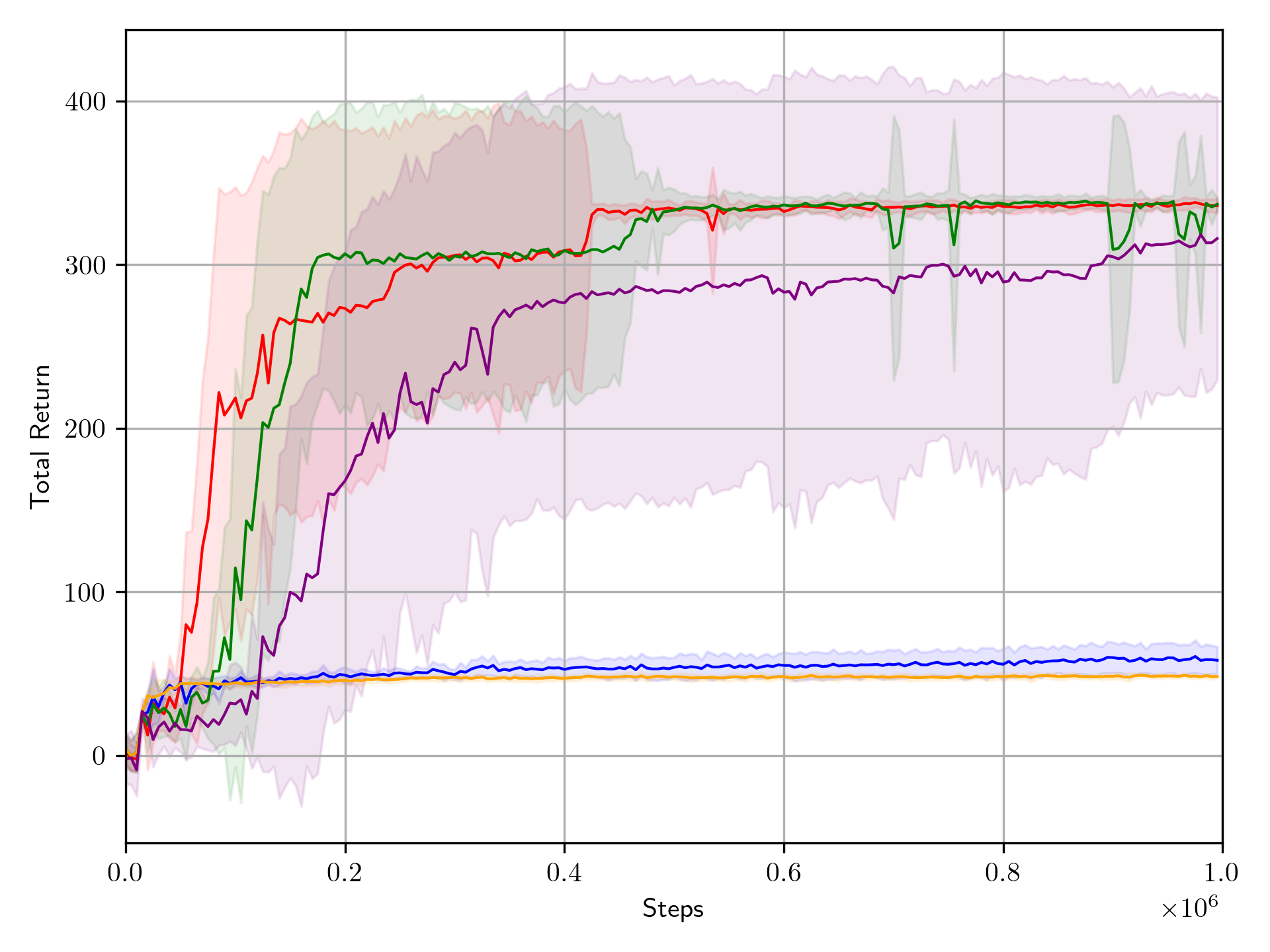
(a) Swimmer

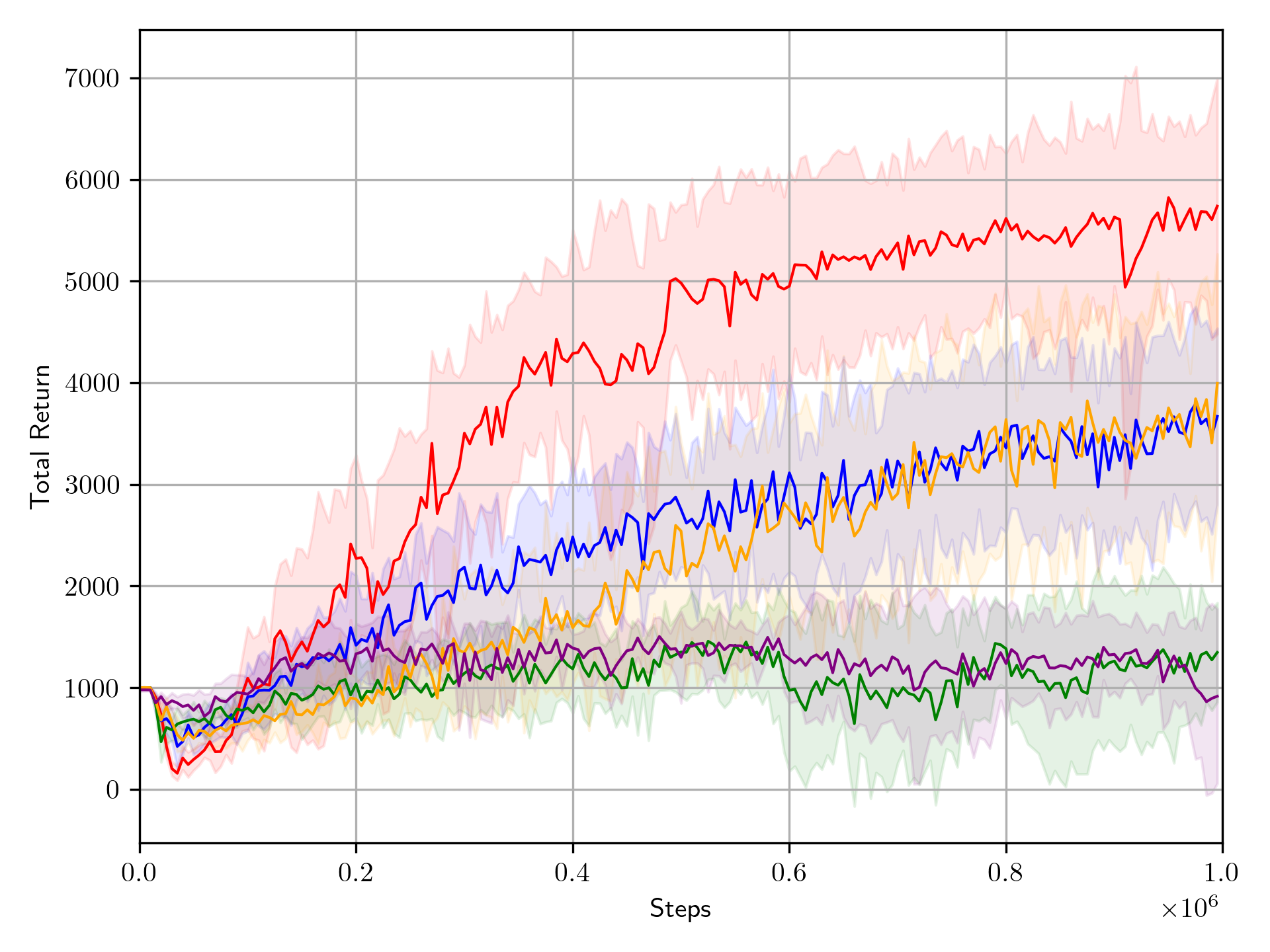
(b) Ant

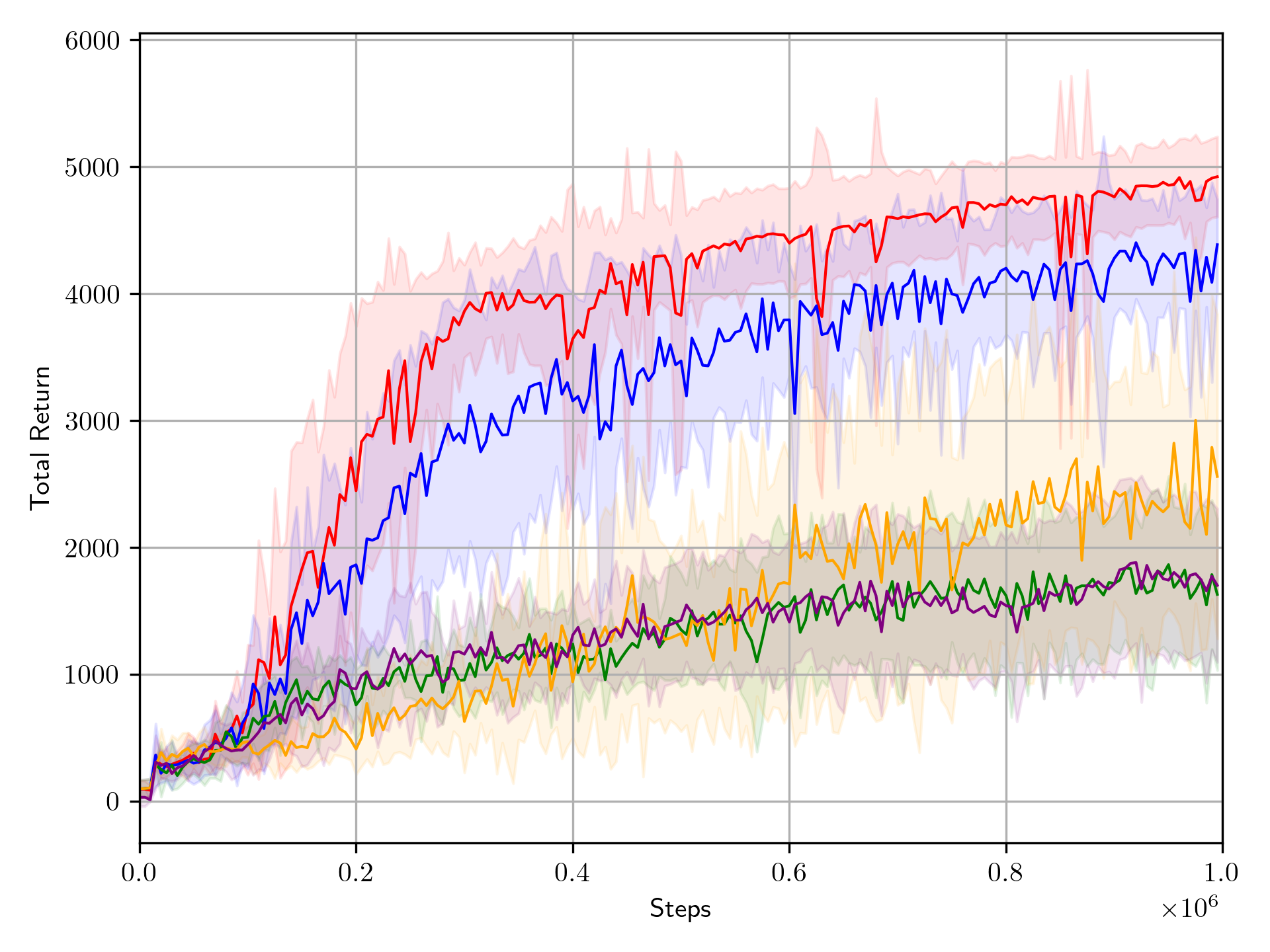
(c) Walker2d

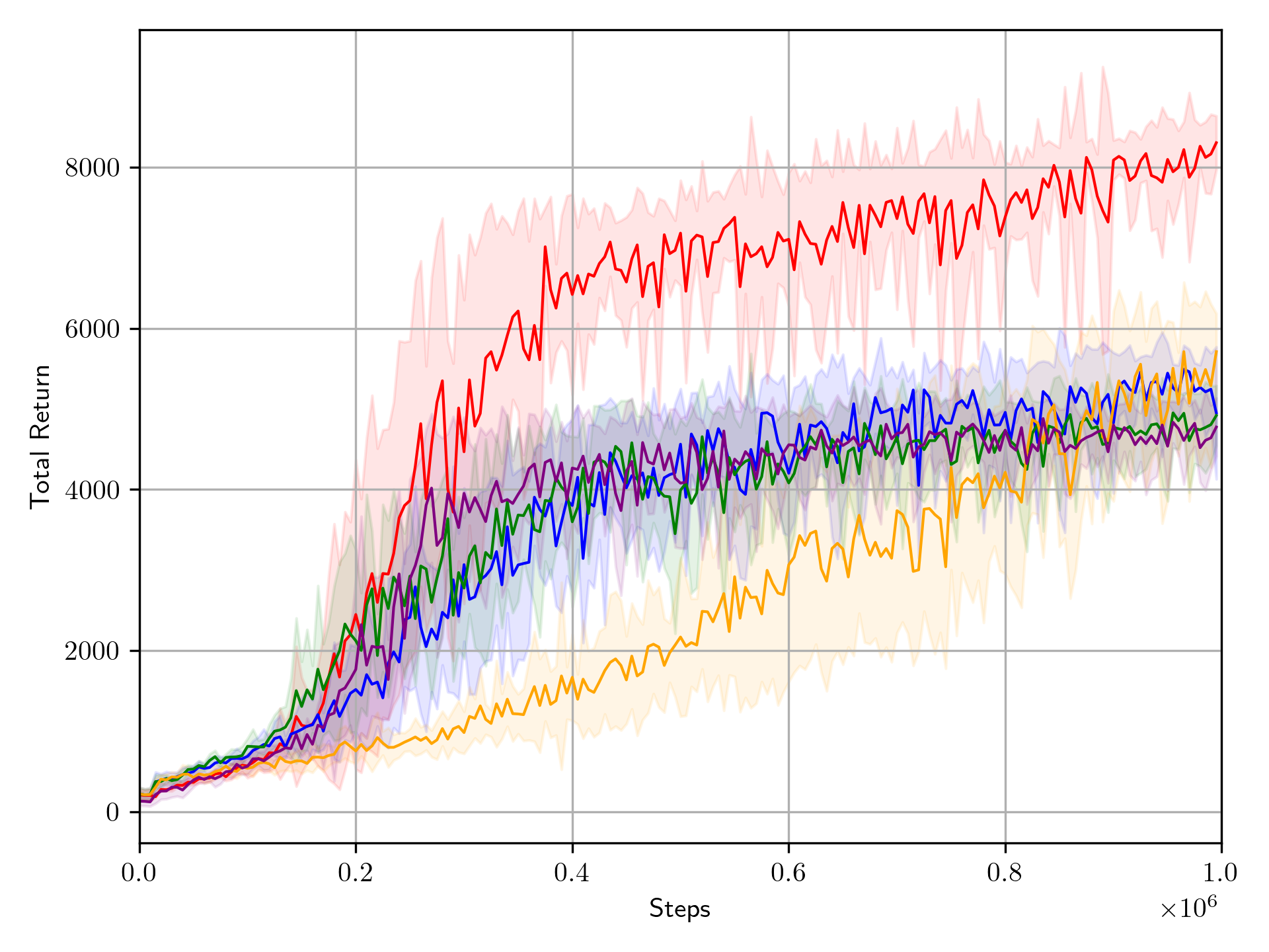
(d) Humanoid

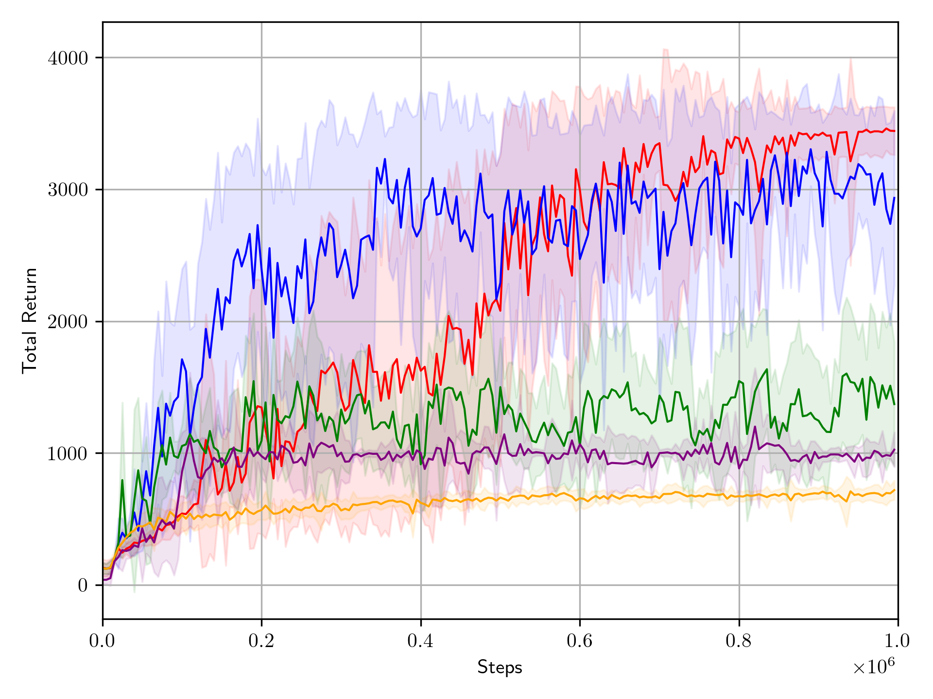
(e) Hopper

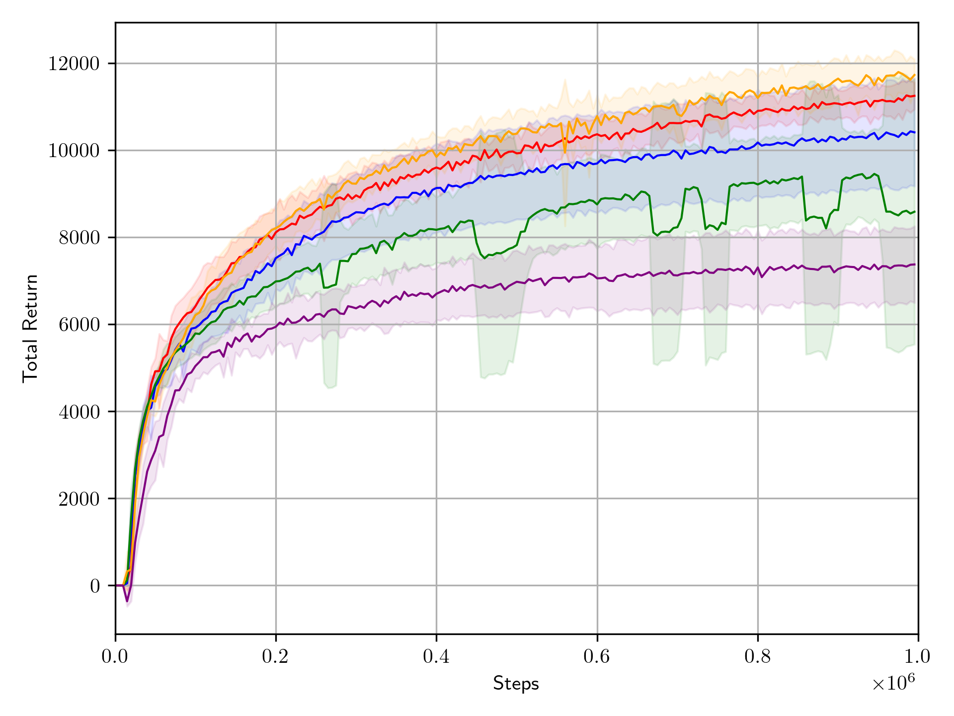
(f) HalfCheetah

Figure 1: Learning curves for the Gymnasium’s Mujoco tasks. The horizontal axis represents Steps, and the vertical axis represents the evaluation value (total_return). Lines and shades represent the mean and standard deviation of the evaluation values over 10 trials, respectively.

We conducted experiments with 10 different random seed trials for each algorithm, sampling evaluation scores every 5,000 steps. For RVI-SAC and SAC, stochastic policies are treated as deterministic during evaluation. The maximum episode step is limited to 1,000 during training and evaluation. Figure 1 shows the learning curves of RVI-SAC, SAC with various discount rates, and ARO-DDPG. These experiments set the evaluation score as the total return over 1,000 steps. Results of experiments with the evaluation score set as an average reward (total_return / survival_step) are presented in Appendix F.1.

From the results shown in Figure 1, when comparing RVI-SAC with SAC with various discount rates, RVI-SAC demonstrates equal or better performance than SAC with the best discount rate in all environments except HalfCheetah. A notable observation is from the Swimmer environment experiments (Figure 1(a)). SAC’s recommended discount rate of $\gamma=0.99$ (Haarnoja et al., 2018a, b) performs better than the other rates in environments other than Swimmer. However, a larger discount rate of $\gamma=0.999$ is required in the Swimmer environment. However, setting a large discount rate can lead to destabilization of learning and slow convergence (Fujimoto et al., 2018; Dewanto & Gallagher, 2021), and indeed, in the environments other than Swimmer, a setting of $\gamma=0.999$ shows lower performance. Compared to SAC, RVI-SAC shows the same performance as SAC ($\gamma=0.999$) in the Swimmer environment and equal or better than SAC ($\gamma=0.99$) in the other environments. This result suggests that while traditional SAC using a discount rate may be significantly impacted by the choice of discount rate, RVI-SAC using the average reward resolves this issue.

When comparing RVI-SAC with ARO-DDPG, RVI-SAC shows higher performance in all environments. SAC has improved performance over methods using deterministic policies by introducing the concept of Maximum Entropy Reinforcement Learning. Similarly, it can be considered that the introduction of this concept to RVI-SAC is the primary reason for RVI-SAC’s superior performance over ARO-DDPG.

4.2 Design evaluation

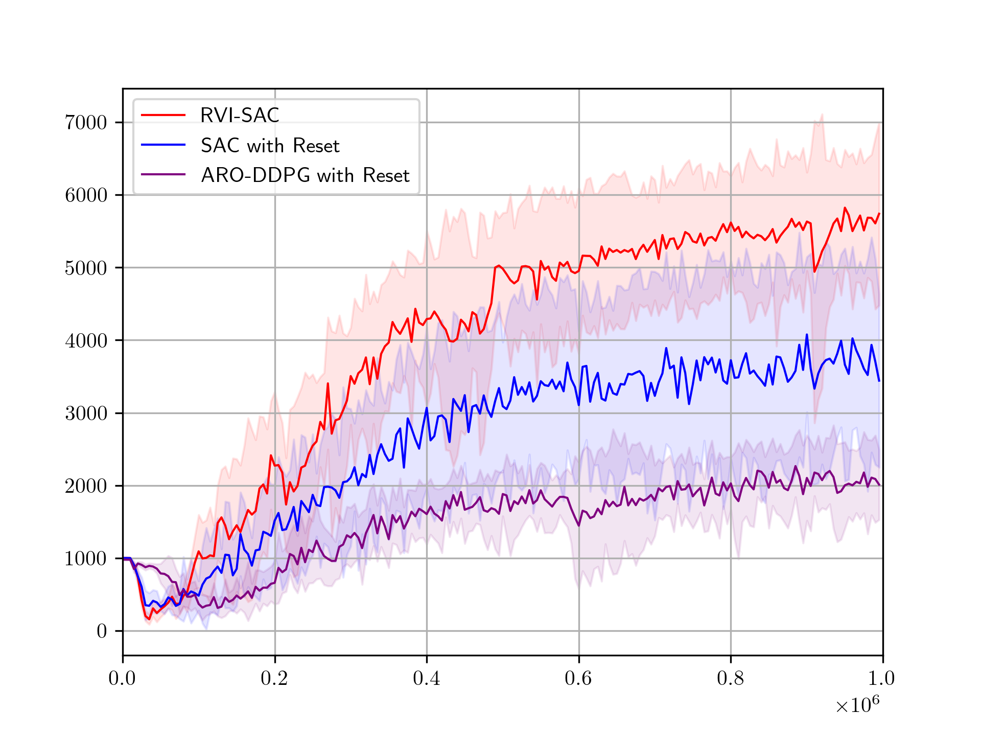
(a) Performance Comparison of RVI-SAC, SAC with automatic Reset Cost adjustment, and ARO-DDPG with automatic Reset Cost adjustment

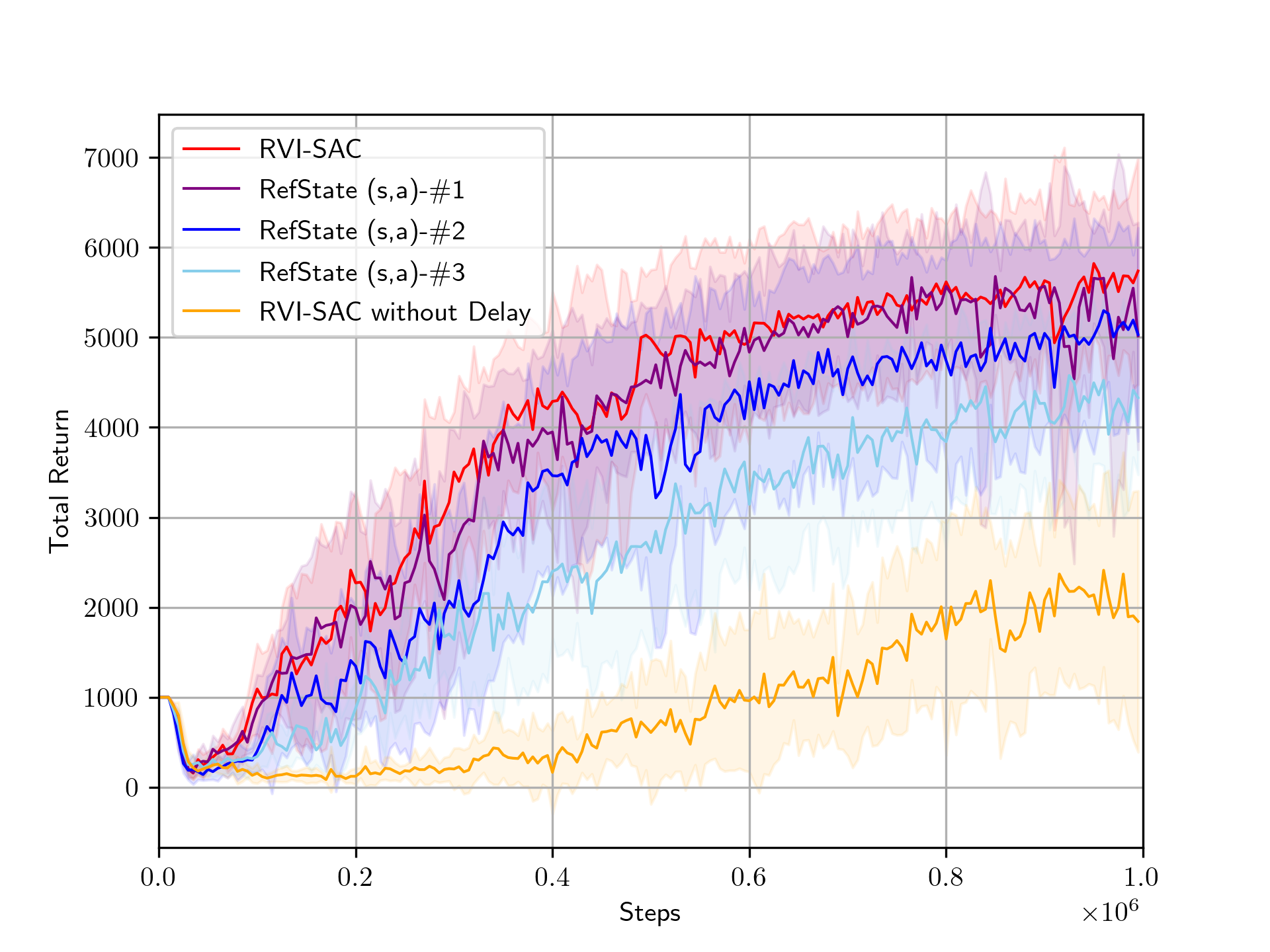
(b) Ablation Study of Delayed f(Q) Update

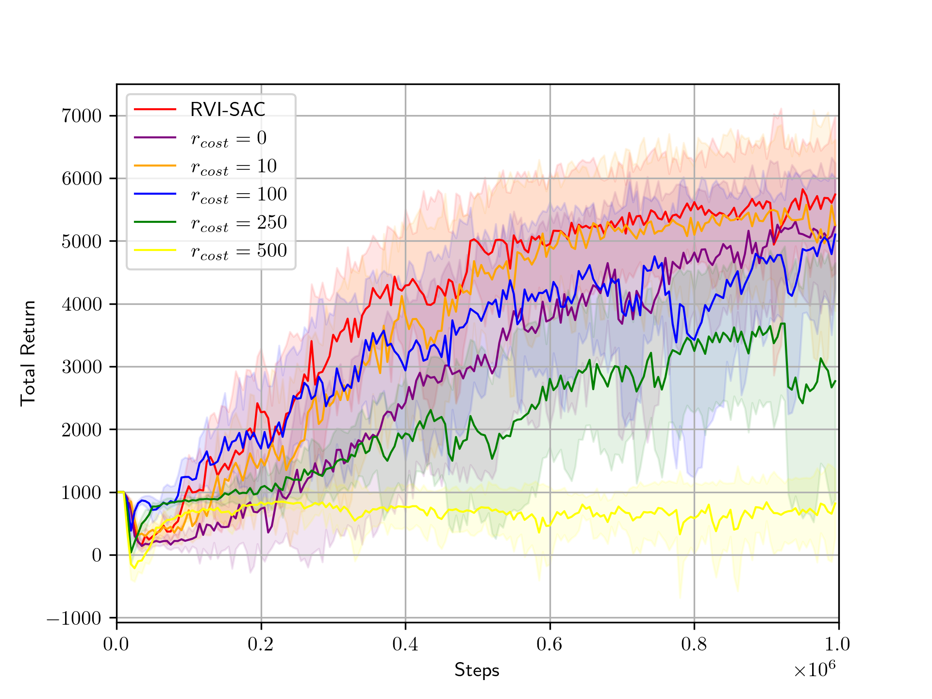
(c) Performance Comparison of RVI-SAC and RVI-SAC with Fixed Reset Cost ($r_{\text{cost}}=0,10,100,250,500$)

Figure 2: Experimental results demonstrating the effectiveness of each component of RVI-SAC. All three graphs represent learning curves on the Ant environment.

In the previous section, we demonstrated that RVI-SAC overall exhibits better performance compared to SAC using various discount rates and ARO-DDPG. In this section, we show how each component of RVI-SAC contributes to the overall performance.

Performance Comparison of RVI-SAC, SAC with automatic Reset Cost adjustment and ARO-DDPG with automatic Reset Cost adjustment

Since RVI-SAC introduces the automatic Reset Cost adjustment, RVI-SAC uses a different reward structures from that used in SAC and ARO-DDPG in which the reward is set to zero after termination. To compare the performance of RVI-SAC, SAC and ARO-DDPG under the same reward structure, we conduct comparative experiments with RVI-SAC, SAC with the automatic Reset Cost adjustment (SAC with Reset) and ARO-DDPG with the automatic Reset Cost adjustment(ARO-DDPG with Reset). Figure 2(a) shows the learning curves of these experiments in the Ant environment. (Results for other environments are shown in Appendix F.2). Here, the discount rate of SAC is set to $\gamma=0.99$.

Figure 2(a) demonstrates that RVI-SAC outperforms SAC with automatic Reset Cost adjustment and ARO-DDPG with automatic Reset Cost adjustment. This result suggests that the improved performance of RVI-SAC is not solely due to the different reward structure but also due to the effects of using the average reward criterion.

Ablation Study of Delayed f(Q) Update

In this section, we evaluate the effectiveness of the Delayed f(Q) Update described in Section 3.1. This method stabilizes learning without depending on a specific state/action pair for updating the Q function. To validate the effectiveness of this method, we examine whether the followings are correct: (1) When the function $f(Q)$ is $f(Q)=Q(S,A)$ for state/action pair $(S,A)\in\mathcal{S}\times\mathcal{A}$, the performance depends on the choice of $(S,A)$. (2) When the Q function is updated using Equation 6 directory as $f(Q)$, learning becomes unstable. To examine these, we conducted performance comparisons with three algorithms: (1) RVI-SAC, (2) RefState $(s,a)-\#1,(s,a)-\#2$ and $(s,a)-\#3$ that are RVI-SACs updating the Q functions with $f(Q)=Q(s,a)$, using sampled state/action pairs, $(s,a)-\#1,(s,a)-\#2$ and $(s,a)-\#3$, as Reference States obtained from when agent takes random actions, respectively, (3) RVI-SAC without Delay that is RVI-SAC updating the Q function using Equation 6 directory as $f(Q)$.

Figure 2(b) shows the learning curves for these methods in the Ant environment. Firstly, comparing RVI-SAC with RefState $(s,a)-\#1,(s,a)-\#2$ and $(s,a)-\#3$, except for RefState $(s,a)-\#1$, the methods using Reference States show lower performance than RVI-SAC. Furthermore, comparing the results of RefState $(s,a)-\#1,(s,a)-\#2$ and $(s,a)-\#3$, it suggests that performance depends on the choice of Reference State. These results suggest the effectiveness of RVI-SAC, which shows good performance without depending on a specific state/action pair. Next, comparing RVI-SAC with RVI-SAC without Delay, which directly uses Equation 6, it is observed that RVI-SAC performs significantly better. This result suggests that, in RVI-SAC, implementing the Delayed f(Q) Update contributes to stabilizing the learning process, thereby achieving higher performance. It indicates the effectiveness of the Delayed f(Q) Update, aiming at stabilizing updates of the Q-function.

RVI-SAC with Fixed Reset Cost

To demonstrate the effectiveness of the Automatic Reset Cost Adjustment, we compare the performance of RVI-SAC and RVI-SAC with fixed Reset Costs in the Ant environment. Figure 2(c) shows the learning curves of RVI-SAC and RVI-SAC with fixed Reset Costs, $r_{\text{cost}}=0,10,100,250,500$. These results show that settings other than the optimal fixed Reset Cost of $r_{\text{cost}}=10$ for this environment decrease performance. Moreover, the performance of RVI-SAC with fixed Reset Costs is highly dependent on its setting. This result suggests the effectiveness of the automatic adjustment of Reset Cost, which does not require specific settings.

5 Related Works

The importance of using the average reward criterion in continuing tasks has been suggested. Blackwell (1962) showed that a Blackwell optimal policy $\pi^{*}$ maximizes the average reward exists, and that, for any discount reward criterion satisfying $\gamma\geq\gamma^{*}$, the optimal policy coincides with the Blackwell optimal policy. However, Dewanto & Gallagher (2021) demonstrated that setting a high discount rate to satisfy $\gamma\geq\gamma^{*}$ can slow down convergence, and a lower discount rate may lead to a sub-optimal policy. Additionally, they noted various benefits of directly applying the average reward criterion to recurrent MDPs. Naik et al. (2019) pointed out that discounted reinforcement learning with function approximation is not an optimization problem, and the optimal policy is not well-defined.

Although there are fewer studies on tabular Q-learning methods and theoretical analyses for the average reward criterion compared to those for the discounted reward criterion, several notable works exist (Schwartz, 1993; Singh, 1994; Abounadi et al., 2001; Wan et al., 2020; Yang et al., 2016) . RVI Q-learning, which forms the foundational idea of our proposed method, was proposed by Abounadi et al. (2001) and generalized by Wan et al. (2020) with respect to the function $f$. Differential Q-learning (Wan et al., 2020) is a special case of RVI Q-learning. The asymptotic convergence of these methods in weakly communicating MDPs has been established by Wan & Sutton (2022).

Several methods focusing on function approximation for average reward criterion have been proposed (Saxena et al., 2023; Abbasi-Yadkori et al., 2019; Zhang & Ross, 2021; Ma et al., 2021; Zhang et al., 2021a, b). A notable study by Saxena et al. (2023) extended DDPG to the average reward criterion and demonstrated performance using dm-control’s Mujoco tasks. This work is deeply relevant to our proposed method. This research provides asymptotic convergence and finite time analysis in a linear function approximation. Another contribution is POLITEX (Abbasi-Yadkori et al., 2019), which updates a policy using a Boltzmann distribution over the sum of action-value estimates from a prior policy. POLITEX demonstrated performance using an Atari’s Ms Pacman. ATRPO (Zhang & Ross, 2021) and APO (Ma et al., 2021) update a policy based on policy improvement bounds to the average reward setting within an on-policy framework. ATRPO and APO demonstrated performance using OpenAI Gym’s Mujoco tasks.

6 Conclusion

In this paper, we proposed RVI-SAC, a novel off-policy DRL method with the average reward criterion. RVI-SAC is composed of three components. The first component is the Critic update based on RVI Q-learning. We did not simply extend RVI Q-learning to the Neural Network method, but introduced a new technique called Delayed f(Q) Update, enabling stable learning without dependence on a Reference State. Additionally, we proved the asymptotic convergence of this method. The second component is the Actor update using the Average Reward Soft Policy Improvement Theorem. The third component is the automatic adjustment of the Reset Cost to apply average reward reinforcement learning to locomotion tasks with termination. We applied RVI-SAC to the Gymnasium’s Mujoco tasks, and demonstrated that RVI-SAC showed competitive performance compared to existing methods.

For future work, on the theoretical side, we consider to provide asymptotic convergence and finite-time analysis of the proposed method using a linear function approximator. On the experimental side, we plan to compare the performance of RVI-SAC using benchmark tasks other than Mujoco tasks and compare it with average reward on-policy methods such as APO (Ma et al., 2021).

Impact Statement

This paper presents work whose goal is to advance the field of Reinforcement Learning. There are many potential societal consequences of our work, none which we feel must be specifically highlighted here.

Appendix A Mathematical Notations

In this paper, we utilize the following mathematical notations:

• $e$ denotes a vector with all elements being 1.

• $D_{\text{KL}}(p|q)$ represents the Kullback-Leibler divergence, defined between probability distributions $p$ and $q$ as $D_{\text{KL}}(p|q)=\sum_{x}p(x)\log\frac{p(x)}{q(x)}$.

• Here, $\mathbbm{1}(\text{``some condition"})$ is an indicator function, taking the value $1$ when “some condition” is satisfied, and $0$ otherwise.

• $\|\cdot\|_{\infty}$ denotes the sup-norm.

Appendix B Overall RVI-SAC algorithm and implementation

Algorithm 1 RVI-SAC

1:  Initialize:Q-Network parameters $\phi_{1},\phi_{2},\phi_{1}^{\prime},\phi_{2}^{\prime}$, Delayed $f(Q)$ update parameter $\xi$, Policy-Network parameters $\theta$, Temperature parameter $\alpha$, Q-Network parameters for reset $\phi_{\text{reset}},\phi_{\text{reset}}^{\prime}$, Delayed $f(Q)$ update parameter $\xi_{\text{reset}}$ for reset, and Reset Cost $r_{\text{cost}}$.

2:  for each iteration do

3:     Sample action $a\sim\pi(\cdot|s)$

4:     Sample next state $s^{\prime}\sim p(\cdot|s,a)$ and reward $r$

5:     if $s^{\prime}\notin\mathcal{S}_{\text{term}}$ then

6:       Store transition $(s,a,r,s^{\prime},\text{is\_reset\_step}=\text{false})$ in replay buffer $\mathcal{D}$

7:     else if $s^{\prime}\in\mathcal{S}_{\text{term}}$ then

8:       Reset environment to initial state $s_{0}$

9:       Store transition $(s,a,r,s_{0},\text{is\_reset\_step}=\text{true})$ in replay buffer $\mathcal{D}$

10:     end if

11:     Sample a mini-batch $\mathcal{B}$ from $\mathcal{D}$

12:     Update $\phi_{1},\phi_{2}$ by minimizing Q-Network loss $J(\phi_{i})$ (Eq. 17)

13:     Update $\xi$ using delayed f(Q) update method (Eq. 18)

14:     Update $\phi_{\text{reset}}$ by minimizing Reset Q-Network loss $J(\phi_{\text{reset}})$ (Eq. 22)

15:     Update $\xi_{\text{reset}}$ using delayed f(Q) update method (Eq. 23)

16:     Update $\theta$ by minimizing Policy-Network loss $J(\theta)$ (Eq. 20)

17:     Update $\alpha$ by minimizing Temperature Parameter loss $J(\alpha)$ (Eq. 21)

18:     Update $r_{\text{cost}}$ by minimizing Reset Cost loss $J(r_{\text{cost}})$ (Eq. 24)

19:     Update $\phi_{1}^{\prime},\phi_{2}^{\prime},\phi_{\text{reset}}^{\prime}$(Eq. 25)

20:  end for

In this section, based on Sections 3.1, 3.2, and 3.3, we present the overall algorithm of RVI-SAC.

The main parameters to be updated in this algorithm are:

• The parameters $\phi_{1},\phi_{2}$ of the Q-Network and their corresponding target network parameters $\phi_{1}^{\prime},\phi_{2}^{\prime}$,

• The parameter $\xi$ for the Delayed f(Q) Update,

• The parameters $\theta$ of the Policy-Network,

• Additionally, this method introduces automatic adjustment of the temperature parameter $\alpha$, as introduced in SAC-v2(Haarnoja et al., 2018b).

Note that the update of the Q-Network uses the Double Q-Value function approximator (Fujimoto et al., 2018).

In cases where environment resets are needed, the following parameters are also updated:

• The Reset Cost $r_{\text{cost}}$,

• The parameters $\phi_{\text{reset}}$ of the Q-Network for estimating the frequency of environment resets and their corresponding target network parameters $\phi^{\prime}_{\text{reset}}$,

• The parameter $\xi_{\text{reset}}$ for the Delayed f(Q) Update.

The Q-Network used to estimate the frequency of environment resets is not directly used in policy updates, therefore the Double Q-Value function approximator is not employed for it.

From Sections 3.1 and 3.2, the parameters $\phi_{1},\phi_{2}$ of the Q-Network are updated by minimizing the following loss function:

$$J(\phi_{i})=\frac{1}{|\mathcal{B}|}\sum_{(s,a,r,s^{\prime},\text{is\_reset\_step})\in\mathcal{B}}\left(Y(s,a,r,s^{\prime},\text{is\_reset\_step})-Q_{\phi_{i}}(s,a)\right)^{2},\ i=1,2,$$ (17)

where

$$Y(s,a,r,s^{\prime},\text{is\_reset\_step})=\hat{r}-\xi+\min_{j=1,2}Q_{\phi^{\prime}_{j}}(s^{\prime},a^{\prime})-\alpha\log\pi_{\theta}(a^{\prime}|s^{\prime}),$$

$$\hat{r}=r-r_{\text{cost}}\mathbbm{1}\left(\text{is\_reset\_step}\right),a^{\prime}\sim\pi_{\theta}(\cdot|s^{\prime}).$$

Note that $\hat{r}$ is the reward penalized by the Reset Cost. $\xi$ is updated as follows using the parameter $\kappa$, based on the Delayed f(Q) update:

$$\xi\leftarrow\xi+\kappa\left(f(Q_{\phi^{\prime}}^{\text{ent}};\mathcal{B})-\xi\right),$$ (18)

$$Q_{\phi^{\prime}}^{\text{ent}}(s,a):=Q_{\phi^{\prime}}(s,a)-\alpha\log\pi_{\theta}(a|s).$$

$Q_{\phi^{\prime}}^{\text{ent}}(s,a)$ represents the entropy augmented Q function as in Equation 15. For a function $Q:\mathcal{S}\times\mathcal{A}\rightarrow\mathbb{R}$, $f(Q;\mathcal{B})$ is calculated as follows:

$$f(Q;\mathcal{B})=\frac{1}{|\mathcal{B}|}\sum_{(s,a,r,s^{\prime},\text{is\_reset\_step})\in\mathcal{B}}Q(s^{\prime},a^{\prime}),$$ (19)

$$a^{\prime}\sim\pi_{\theta}(\cdot|s^{\prime}).$$

The parameters $\theta$ of the Policy-Network is updated to minimize the following loss function, as described in Section 3.2, using the same method as in SAC:

$$J(\theta)=\frac{1}{|\mathcal{B}|}\sum_{(s,a,r,s^{\prime},\text{is\_reset\_step})\in\mathcal{B}}\left(\alpha\log\pi_{\theta}(a^{\prime}|s)-\min_{j=1,2}Q_{\phi_{j}}(s,a^{\prime})\right),a^{\prime}\sim\pi_{\theta}(\cdot|s).$$ (20)

Furthermore, since the theory and update method for the temperature parameter $\alpha$ do not depend on the discount rate $\gamma$, it is updated in the same way as in SAC:

$$J(\alpha)=\frac{1}{|\mathcal{B}|}\sum_{(s,a,r,s^{\prime},\text{is\_reset\_step})\in\mathcal{B}}\alpha\left(-\log\pi_{\theta}(a^{\prime}|s)-\overline{\mathcal{H}}\right),a^{\prime}\sim\pi_{\theta}(\cdot|s).$$ (21)

where $\overline{\mathcal{H}}$ is the entropy target.

The parameters $\phi_{\text{reset}}$ of the Q-Network for estimating the frequency of environment resets are updated to minimize the following loss function,

$$J(\phi_{\text{reset}})=\frac{1}{|\mathcal{B}|}\sum_{(s,a,r,s^{\prime},\text{is\_reset\_step})\in\mathcal{B}}\left(Y_{\text{reset}}(s,a,r,s^{\prime},\text{is\_reset\_step})-Q_{\phi_{\text{reset}}}(s,a)\right)^{2},$$ (22)

$$Y_{\text{reset}}(s,a,r,s^{\prime},\text{is\_reset\_step})=\mathbbm{1}\left(\text{is\_reset\_step}\right)-\xi_{\text{reset}}+Q_{\phi^{\prime}_{\text{reset}}}(s^{\prime},a^{\prime}),$$

$$a^{\prime}\sim\pi_{\theta}(\cdot|s^{\prime}),$$

and $\xi_{\text{reset}}$ is updated as

$$\xi_{\text{reset}}\leftarrow\xi_{\text{reset}}+\kappa\left(f(Q_{\phi^{\prime}_{\text{reset}}};\mathcal{B})-\xi_{\text{reset}}\right)$$ (23)

using the calculation for $f(Q_{\phi^{\prime}_{\text{reset}}};\mathcal{B})$ provided in Equation 19.

When using $\xi_{\text{reset}}$ as an estimator for $\rho_{\text{reset}}^{\pi}$, the Reset Cost $r_{\text{cost}}$ is updated to minimize the following loss function, as described in Section 3.3:

$$J(r_{\text{cost}})=-r_{\text{cost}}\left(\xi_{\text{reset}}-\epsilon_{\text{reset}}\right).$$ (24)

The parameters of the target network $\phi_{1}^{\prime},\phi_{2}^{\prime},\phi^{\prime}_{\text{reset}}$ are updated according to the parameter $\tau$ as follows:

$$\phi_{1}^{\prime}\leftarrow\tau\phi_{1}+(1-\tau)\phi_{1}^{\prime}$$ (25)

$$\phi_{2}^{\prime}\leftarrow\tau\phi_{2}+(1-\tau)\phi_{2}^{\prime}$$

$$\phi_{\text{reset}}^{\prime}\leftarrow\tau\phi_{\text{reset}}+(1-\tau)\phi_{\text{reset}}^{\prime}$$

The pseudocode for the entire algorithm is presented in Algorithm 1.

Appendix C Convergence Proof of RVI Q-learning with Delayed $f(Q)$ Update

In this section, we present the asymptotic convergence of the Delayed f(Q) Update algorithm, as outlined in Equation 10. This algorithm is a two-time-scale stochastic approximation (SA) and updates the Q-values and offsets in average reward-based Q-learning at different time scales. This approach is similar to the algorithm proposed in Gosavi (2004). Moreover, the convergence discussion in this section largely draws upon the discussions in Konda & Borkar (1999); Gosavi (2004).

C.1 Proposed algorithm

In this section, we reformulate the algorithm for which we aim to prove convergence.

Consider an MDP with a finite state-action space that satisfies Assumption 2.1. For all $(s,a)\in\mathcal{S}\times\mathcal{A}$, let us define the update equations for a scalar sequence ${\xi_{k}}$ and a tabular Q function ${Q_{k}}$ as follows:

$$\xi_{k+1} = \xi_{k}+a(k)\left(f(Q_{k};X_{k})-\xi_{k}\right),$$ (26)

$$Q_{k+1}(s,a) = Q_{k}(s,a)+b(\nu(k,s,a))\left(r(s,a)-g_{\eta}(\xi_{k})+\max_{a^{\prime}}Q_{k}(s^{\prime},a^{\prime})-Q_{k}(s,a)\right)\mathbbm{1}\left((s,a)=\phi_{k}\right).$$ (27)

$g_{\eta}(\cdot)$ is a clip function newly added from Equation 10 to ensure the convergence of this algorithm. For any $\eta>0$, it is defined as:

$$g_{\eta}(x)=\left\{\begin{array}[]{lll}\|r\|_{\infty}+\eta&\text{ for }&x\geq\|r\|_{\infty}+\eta,\\ x&\text{ for }&-\|r\|_{\infty}-\eta<x<\|r\|_{\infty}+\eta,\\ -\|r\|_{\infty}-\eta&\text{ for }&x\leq-\|r\|_{\infty}-\eta.\end{array}\right.$$ (28)

At discrete time steps $k$, $\phi_{k}$ denotes the sequence of state/action pairs updated at time $k$, and $s^{\prime}$ represents the next state sampled when the agent selects action $a$ in state $s$. The function $\nu(k,s,a)$ counts the number of updates to $Q(s,a)$ up to time $k$, defined as $\nu(k,s,a)=\sum_{m=0}^{k}\mathbbm{1}\left((s,a)=\phi_{m}\right)$. The functions $a(\cdot)$ and $b(\cdot)$ represent the step-size. For the random variable $X_{k}$ and the function $f(\cdot;\cdot)$, we introduce the following assumption within the increasing $\sigma$-field $\mathcal{F}_{k}=\sigma(\xi_{n},Q_{n},n\leq k,w_{n,1},w_{n,2},n<k)$, where $w_{n,1},w_{n,2}$ are defined in Equation 35.

Assumption C.1.

It holds that

$${{\mathbb{E}}}_{\begin{subarray}{c}\end{subarray}}\left[f(Q_{k};X_{k})-f(Q_{k})\mid\mathcal{F}_{k}\right]=0,$$

and for some constant $K$,

$${{\mathbb{E}}}_{\begin{subarray}{c}\end{subarray}}\left[\|f(Q_{k};X_{k})-f(Q_{k})\|^{2}\mid\mathcal{F}_{k}\right]<K(1+\|Q_{k}\|^{2}).$$

This assumption is obviously satisfied when $f$ is set as in Equation 7.

C.2 The ODE framework and stochastic approximation(SA)

In this section, we revisit the convergence results for SA with two update equations on different time scales, as demonstrated in Konda & Borkar (1999); Gosavi (2004).

The sequences $\left\{x_{k}\right\}$ and $\left\{y_{k}\right\}$ are in $\mathbb{R}^{n}$ and $\mathbb{R}^{l}$, respectively. For $i=1,\ldots,n$ and $j=1,\ldots,l$, they are generated according to the following update equations:

$$x^{i}_{k+1} = x^{i}_{k}+a(\nu_{1}(k,i))\left(h^{i}\left(x_{k},y_{k}\right)+w^{i}_{k,1}\right)\mathbbm{1}\left(i=\phi_{k,1}\right),$$ (29)

$$y^{j}_{k+1} = y^{j}_{k}+b(\nu_{2}(k,j))\left(f^{j}\left(x_{k},y_{k}\right)+w^{j}_{k,2}\right)\mathbbm{1}\left(j=\phi_{k,2}\right),$$ (30)

where the superscripts in each vector represent vector indices, and $\left\{\phi_{k,1}\right\}$ and $\left\{\phi_{k,2}\right\}$ are stochastic processes taking values on the sets $S_{1}=\{1,2,\ldots,n\}$ and $S_{2}=\{1,2,\ldots,l\}$, respectively. The functions $h(\cdot,\cdot)$ and $f(\cdot,\cdot)$ are arbitrary functions of $(x_{k},y_{k})$. The terms $w_{k,1},w_{k,2}$ represent noise components, and $\nu_{1},\nu_{2}$ are defined as:

$$\nu_{1}(k,i) =\sum_{m=0}^{k}\mathbbm{1}\left(i=\phi_{m,1}\right),$$

$$\nu_{2}(k,j) =\sum_{m=0}^{k}\mathbbm{1}\left(j=\phi_{m,2}\right).$$

In the context of the proposed method (Equations 26 and 27), $x_{k}$ corresponds to $\xi_{k}$, and $y_{k}$ corresponds to $Q_{k}$. This implies that $n$ is 1, and $l$ is equal to the number of state/action pairs. Consequently, $\nu_{1}(k,i)$ corresponds $k$ due to $n=1$, and $\nu_{2}(k,j)$ corresponds to $\nu(k,s,a)$.

We assume the following assumptions for this SA:

Assumption C.2.

The functions $h$ and $f$ are Lipschitz continuous.

Assumption C.3.

There exist $\Delta>0$ such that

$$\liminf_{k\rightarrow\infty}\frac{\nu_{1}(k,i)}{k+1}\geq\Delta,$$

and

$$\liminf_{k\rightarrow\infty}\frac{\nu_{2}(k,j)}{k+1}\geq\Delta.$$

almost surely, for all $i=1,2,\ldots,n$ and $j=1,2,\ldots,l$. Furthermore, if, for $a(\cdot),b(\cdot)$ and $x>0$,

$$N(k,x) =\min\left\{m>k:\sum_{i=k+1}^{m}\overline{a}(i)\geq x\right\},$$

$$N^{\prime}(k,x) =\min\left\{m>k:\sum_{i=k+1}^{m}\overline{b}(i)\geq x\right\},$$

where $\overline{a}(i)=a(\nu_{1}(i,\phi_{i,1})),\overline{b}(i)=b(\nu_{2}(i,\phi_{i,2}))$ , then the limits

$$\lim_{k\rightarrow\infty}\frac{\sum_{m=\nu_{1}(k,i^{\prime})}^{\nu_{1}\left(N(k,x),i^{\prime}\right)}a(m)}{\sum_{m=\nu_{1}(k,i)}^{\nu_{1}(N(k,x),i)}a(m)},$$

$$\lim_{k\rightarrow\infty}\frac{\sum_{m=\nu_{2}(k,j^{\prime})}^{\nu_{2}\left(N^{\prime}(k,x),j^{\prime}\right)}b(m)}{\sum_{m=\nu_{2}(k,j)}^{\nu_{2}\left(N^{\prime}(n,x),j\right)}b(m)}$$

exist almost surely for all $i,i^{\prime},j,j^{\prime}$ (Together, these conditions imply that the components are updated “comparably often” in an “evenly spread” manner.)

Assumption C.4.

Let $c(k)$ be $a(k)$ or $b(k)$. The standard conditions for convergence that $c(k)$ must satisfy are as follows:

• $\sum_{k}c(k)=\infty,\sum_{k}c^{2}(k)<\infty$

• For $x\in(0,1)$,

  $$\sup_{k}c([xk])/c(k)<\infty,$$

  where $[\cdots]$ stands for the integer part of “…”.

• For $x\in(0,1)$ and $A(k)=\sum_{i=0}^{k}c(i)$,

  $$A([yk])/A(k)\rightarrow 1,$$

  uniformly in $y\in[x,1]$.

Assumption C.5.

In addition to Assumption C.4, the following conditions must be satisfied:

$$\lim_{k\rightarrow\infty}\sup\frac{b(k)}{a(k)}=0$$

.

Assumption C.6.

Let $\mathcal{F}_{k}=\sigma(x_{n},y_{n},n\leq k,w_{n,1},w_{n,2},n<k)$ be a increasing $\sigma$-field. For some constants ,$K_{1}$ and $K_{2}$, the following condition is satisfied:

$${{\mathbb{E}}}_{\begin{subarray}{c}\end{subarray}}\left[w_{k,1}\mid\mathcal{F}_{k}\right]=0,$$

$${{\mathbb{E}}}_{\begin{subarray}{c}\end{subarray}}\left[\left\|w_{k,1}\right\|^{2}\mid\mathcal{F}_{k}\right]\leq K_{1}(1+\left\|x_{k}\right\|^{2}+\left\|y_{k}\right\|^{2}),$$

and

$${{\mathbb{E}}}_{\begin{subarray}{c}\end{subarray}}\left[w_{k,2}\mid\mathcal{F}_{k}\right]=0,$$

$${{\mathbb{E}}}_{\begin{subarray}{c}\end{subarray}}\left[\left\|w_{k,2}\right\|^{2}\mid\mathcal{F}_{k}\right]\leq K_{2}(1+\left\|x_{k}\right\|^{2}+\left\|y_{k}\right\|^{2}).$$

Assumption C.7.

The iterations of $x_{k}$ and $y_{k}$ are bounded.

Assumption C.8.

For all $y\in\mathbb{R}^{l}$, the ODE

$$\dot{x}_{t}=h(x_{t},y)$$ (31)

has an asymptotically stable critical point $\lambda(y)$ such that the map $\lambda$ is Lipschitz continuous.

Assumption C.9.

The ODE

$$\dot{y}_{t}=f(\lambda(y_{t}),y_{t})$$ (32)

has a global asymptotically stable critical point $y^{*}$.

Note that, $t$ represents continuous time.

From Konda & Borkar (1999); Gosavi (2004), the following theorem holds:

Theorem C.10.

Let Assumption C.2 to C.9 hold. Then, $\{(x_{k},y_{k})\}$ converges almost surely to $\left(\lambda\left(y^{*}\right),y^{*}\right)$.

This theorem is slightly different from the problem setting for the convergence of two-time-scale SA as described in Konda & Borkar (1999). In Konda & Borkar (1999), it is assumed that a projection mapping $P$ is applied to the entire right-hand side of the update equation for $y_{k}$ (Equation 30), such that $P(x)=y,\ y\in G,|x-y|=\inf_{z\in G}|z-x|$ for some closed convex set $G$. Instead of this setting, we assume in Assumption C.7 that $y_{k}$ is bounded. With this assumption, there exists a projection mapping $P$ that, even if applied to the right-hand side of Equation 30, would not affect the values of $y_{k}$. Therefore, Theorem C.10 is essentially encompassed by the results in Konda & Borkar (1999).

C.3 Proof

We show the convergence of the proposed method by verifying that each of the assumptions presented in the previous section is satisfied.

First, we prepare ODEs related to the update equations 26 and 27. The mappings $H_{1}$ and $H_{2}$ are defined as follows:

$$H_{1}(\xi,Q) =f(Q),$$

$$H_{2}(\xi,Q)(s,a) =r(s,a)-g_{\eta}(\xi)+\sum_{s^{\prime}}p(s^{\prime}|s,a){\max_{a^{\prime}}Q(s^{\prime},a^{\prime})}.$$

We rewrite Equations 26 and 27 using the mappings $H_{1}$ and $H_{2}$ as follows:

$$\xi_{k+1} = \xi_{k}+a(k)\left(H_{1}(\xi_{k},Q_{k})-\xi_{k}+w_{k,1}\right),$$ (33)

$$Q_{k+1}(s,a) = Q_{k}(s,a)+b(\nu(k,s,a))\left(H_{2}(\xi_{k},Q_{k})(s,a)-Q_{k}(s,a)+w_{k,2}(s,a)\right)\mathbbm{1}\left((s,a)=\phi_{k}\right).$$ (34)

Here, the noise terms $w_{k,1}$ and $w_{k,2}$ are defined respectively as follows:

$$w_{k,1} =f(Q_{k};X_{k})-H_{1}(Q_{k},\xi_{k})=f(Q_{k};X_{k})-f(Q_{k}),$$ (35)

$$w_{k,2}(s,a) =r(s,a)-g_{\eta}(\xi_{k})+\max_{a^{\prime}}Q_{k}(s^{\prime},a^{\prime})-H_{2}(Q_{k},\xi_{k})(s,a).$$

Using $H_{1}$ and $H_{2}$, we define the ODEs related to Equations 26 and 27 (where Equation 36 corresponds to Equation 26, and Equation 37 corresponds to Equation 27) as follows:

$$\dot{\xi}_{t} = H_{1}(\xi_{t},Q)-\xi_{t},\ \ \forall Q$$ (36)

$$\dot{Q}_{t} = H_{2}(\lambda(Q_{t}),Q_{t})-Q_{t}.$$ (37)

C.3.1 Boundness of the iteration (Assumption C.7)

In this section, we show that Assumption C.7 holds for the iterations defined in Equations 26 and 27. To this end, we introduce an assumption for the MDP as introduced in Gosavi (2004)

Assumption C.11.

There exists a state $s$ in the Markov chain such that for some integer $m$, and for all initial states and all stationary policies, $s$ is visited with a positive probability at least once within the first $m$ timesteps.

Under this assumption, the mapping $T$ defined as

$$T(Q)(s,a)=r(s,a)+\sum_{s^{\prime}}p(s^{\prime}|s,a){\max_{a^{\prime}}Q(s^{\prime},a^{\prime})}$$ (38)

is shown to be a contraction mapping with respect to a certain weighted sup-norm. (For proof, see Appendix A.5 in Gosavi (2004)). This means that there exists a vector $\gamma$ and a scalar $\delta\in(0,1),D>0$, such that

$$\|T(Q)\|_{\gamma}\leq\delta\|Q\|_{\gamma}+D$$

is satisfied. Here, $|v|_{\gamma}$ is defined as a weighted sup-norm given by

$$\|v\|_{\gamma}=\max_{s,a\in\mathcal{S}\times\mathcal{A}}\frac{|v(s,a)|}{\gamma(s,a)}.$$

Regarding $H_{2}$, it holds that

$$H_{2}(\xi,Q)(s,a) =T(Q)(s,a)-g_{\eta}(\xi)$$

$$\Rightarrow|H_{2}(\xi,Q)(s,a)| \leq|T(Q)(s,a)|+|g_{\eta}(\xi)|,\ \forall s,a.$$

From the definition of $g_{\eta}(\xi)$ (Equation 28), $g_{\eta}(\xi)$ is bounded. Therefore, for some $D_{1}>0$ and for any $\xi$, the following is satisfied:

$$\|H_{2}(\xi,Q)\|_{\gamma} \leq\|T(Q)\|_{\gamma}+D_{1}$$

$$\Rightarrow\|H_{2}(\xi,Q)\|_{\gamma} \leq\delta\|Q\|_{\gamma}+D+D_{1}.$$

Consequently, utilizing the results from (Tsitsiklis, 1994), the iteration expressed in Equation 34, which employs $H_{2}$, maintains the boundedness of $Q_{k}$. Additionally, when $Q_{k}$ is bounded, $f(Q_{k};X_{k})$ is also bounded, thereby ensuring that $\xi_{k}$ remains bounded as well.

C.3.2 Convergence of the ODE (Assumption C.8, C.9)

We verify that Equation 36 satisfies Assumption C.8. The function $H_{1}(\xi,Q)$ in Equation 36 is independent of $\xi$, and when $Q$ is fixed, $H_{1}(\xi,Q)$ becomes a constant. Therefore, it is obvious that Assumption C.8 is satisfied, and we have

$$\lambda(Q)=f(Q).$$

Consequently, we can rewrite Equation 37 as follows:

$$\dot{Q}_{t}=H_{2}(f(Q_{t}),Q_{t})-Q_{t}=T(Q_{t})-g_{\eta}(f(Q_{t}))e-Q_{t}.$$ (39)

Next, we verify Assumption C.9 for Equation 39. To demonstrate the convergence of Equation 39, we introduce the following lemma from Wan et al. (2020):

Lemma C.12.

The following ODE

$$\dot{w}_{t}=T(w_{t})-f(w_{t})e-w_{t}$$ (40)

is globally asymptotically stable and converges to $w_{t}\rightarrow q^{*}$. Here, $q^{*}$ satisfies the optimal Bellman equation (as shown in Equation 4) and the following conditions with respect to the function $f$:

$$q^{*}(s,a) =r(s,a)-\rho^{*}+\sum_{s^{\prime}\in\mathcal{S}}p(s^{\prime}|s,a)\max_{a^{\prime}}q^{*}(s^{\prime},a^{\prime}),$$

$$\rho^{*} =f(q^{*}).$$

For Equation 39, we demonstrate that the following lemma holds:

Lemma C.13.

The ODE shown in Equation 39 is globally asymptotically stable and converges to $Q_{t}\rightarrow q^{*}$. Here, $q^{*}$ is the same as the $q^{*}$ in Lemma C.12.

Proof.

First, from the definition of function $g_{\eta}(\cdot)$ (Equation 28), it is obvious that $g_{\eta}(f(q^{*}))=f(q^{*})$, thus $q^{*}$ is an equilibrium point of the ODE shown in Equation 39.

Next, we show that the ODE presented in Equation 39 satisfies Lyapunov stability. That is, we need to show that, for any given $\epsilon>0$, there exists $\delta>0$ such that if $\|q^{*}-Q_{0}\|_{\infty}\leq\delta$, then it implies $\|q^{*}-Q_{t}\|_{\infty}\leq\epsilon$ for all $t\geq 0$. To demonstrate this, the following lemma is presented:

Lemma C.14.

Let $L$ be the Lipschitz constant of the function $f$. If $\|q^{*}-Q_{0}\|_{\infty}\leq\frac{\eta}{L(1+L)}$, then for the solution $Q_{t}$ of the ODE (Equation 39) and the solution $w_{t}$ of the ODE (Equation 40) with $Q_{0}=w_{0}$, it holds that $Q_{t}=w_{t}$.

Proof.

From Wan et al. (2020), it is known that the following holds for the ODE in Equation 40:

$$\left|\rho^{*}-f(w_{t})\right| =\left|f(q^{*})-f(w_{t})\right|$$

$$\leq L\|q^{*}-w_{t}\|_{\infty}$$

$$\leq L(1+L)\|q^{*}-w_{0}\|_{\infty}.$$

Here, we choose $w_{0}$ such that $\|q^{*}-w_{0}\|_{\infty}\leq\frac{\eta}{L(1+L)}$. Under this condition,

$$\left|\rho^{*}-f(w_{t})\right|\leq\eta$$

$$\Rightarrow\rho^{*}-\eta\leq f(w_{t})\leq\rho^{*}+\eta$$

$$\Rightarrow-\|r\|_{\infty}-\eta\leq f(w_{t})\leq\|r\|_{\infty}+\eta.$$

This result implies that $g_{\eta}(f(w_{t}))=f(w_{t})$ for all $t\geq 0$. Therefore, for the ODE in Equation 39 with $Q_{0}=w_{0}$, it follows that $Q_{t}=w_{t}$. ∎

Given that the ODE in Equation 40 satisfies Lyapunov stability (as shown in Wan et al. (2020)), it follows from Lemma C.14 that, for any $\epsilon$, by choosing $\delta\leq\frac{\eta}{L(1+L)}$, the ODE in Equation 39 also satisfies Lyapunov stability.

To demonstrate global asymptotic stability, we need to show that, for any initial $Q_{0}$, $\lim_{t\rightarrow\infty}\|q^{*}-Q_{t}\|_{\infty}=0$. Setting $w_{0}=Q_{0}$ and defining $v_{t}e=w_{t}-Q_{t}$. Then, we have

$$\dot{v}_{t}e =\dot{w}_{t}-\dot{Q}_{t}$$

$$=T(w_{t})-f(w_{t})e-w_{t}-\left(T(Q_{t})-g_{\eta}(f(Q_{t}))e-Q_{t}\right)$$

$$=T(w_{t})-T(w_{t}-v_{t}e)-\left(f(w_{t})e-g_{\eta}(f(w_{t}-v_{t}e))e\right)-v_{t}e$$

$$=T(w_{t})-T(w_{t})+v_{t}e-\left(f(w_{t})e-g_{\eta}(f(w_{t})-uv_{t})e\right)-v_{t}e$$

$$=-f(w_{t})e+g_{\eta}(f(w_{t})-uv_{t})e.$$

From the definition of $g_{\eta}(\cdot)$, $\dot{v}_{t}$ can be expressed as follows:

$$\dot{v}_{t}=\left\{\begin{array}[]{lll}-f(w_{t})+\|r\|_{\infty}+\eta&\text{ for }&f(w_{t})-uv_{t}\geq\|r\|_{\infty}+\eta,\\ -uv_{t}&\text{ for }&-\|r\|_{\infty}-\eta<f(w_{t})-uv_{t}<\|r\|_{\infty}+\eta,\\ -f(w_{t})-\|r\|_{\infty}-\eta&\text{ for }&f(w_{t})-uv_{t}\leq-\|r\|_{\infty}-\eta.\end{array}\right.$$

Here, we consider a time $T_{\eta^{\prime}}$ that satisfies the following condition for some $0<\eta^{\prime}<\eta$:

$$|\rho^{*}-f(w_{t})| \leq|f(q^{*})-f(w_{t})|$$

$$\leq L\|q^{*}-w_{t}\|_{\infty}$$

$$\leq\eta^{\prime},\ \ \forall t\geq T_{\eta^{\prime}}.$$

(Lemma C.12 ensures the existence of such $T_{\eta^{\prime}}$.) For $t\geq T_{\eta^{\prime}}$, the following holds:

$$-\eta^{\prime} \leq f(w_{t})-\rho^{*} \leq \eta^{\prime}$$

$$\Rightarrow-\|r\|_{\infty}-\eta<\rho^{*}-\eta^{\prime} \leq f(w_{t}) \leq \rho^{*}+\eta^{\prime}<\|r\|_{\infty}+\eta.$$

Therefore, for $v_{t}$, the following holds:

• When $f(w_{t})-uv_{t}\geq\|r\|_{\infty}+\eta\Rightarrow v_{t}\leq\frac{f(w_{t})-\|r\|_{\infty}-\eta}{u}<0$, we have

  $$\dot{v}_{t}=-f(w_{t})+\|r\|_{\infty}+\eta>0$$

• When $-\|r\|_{\infty}-\eta<f(w_{t})-uv_{t}<\|r\|_{\infty}+\eta\Rightarrow\frac{-\|r\|_{\infty}-\eta}{u}<v_{t}<\frac{\|r\|_{\infty}+\eta}{u}$,

  $$\dot{v}_{t}=-uv_{t}$$

• When $f(w_{t})-uv_{t}\leq-\|r\|_{\infty}-\eta\Rightarrow v_{t}\geq\frac{f(w_{t})+\|r\|_{\infty}+\eta}{u}>0$, we have

  $$\dot{v}_{t}=-f(w_{t})-\|r\|_{\infty}-\eta<0$$

Setting the Lyapunov function as $V(v)=\frac{1}{2}v^{2}$, $\dot{V}(v_{t})=v_{t}\dot{v}_{t}$ is such that $\dot{V}(v_{t})=0$ when $v_{t}=0$, and $\dot{V}(v_{t})<0$ when $v_{t}\neq 0$. Thus, from the Lyapunov Second Method, $v=0$ is a globally asymptotically stable point. Therefore, for any initial $v_{T_{\eta^{\prime}}}$, we can achieve $v_{t}\rightarrow 0$, leading to $\lim_{t\rightarrow\infty}\|q^{*}-Q_{t}\|_{\infty}=0$. Hence, the ODE in Equation 39 is globally asymptotically stable at $q^{*}$. ∎

C.3.3 Verification of other assumptions

We verify the remaining assumptions (Assumption C.2, C.3, C.4, C.5 and C.6).

First, regarding Assumption C.2, the function $h$ corresponds to $H_{1}(\xi,Q)-\xi$, and the function $f$ corresponds to $H_{2}(\xi,Q)-Q$. It is clear that all terms constituting these functions are Lipschitz continuous. Therefore, the overall functions are also Lipschitz continuous, satisfying Assumption C.2.

Assumption C.3 concerns the update frequency of elements in the vector being updated during the learning process, which is commonly used in asynchronous SA (Borkar, 2009; Abounadi et al., 2001; Wan et al., 2020). Since $\xi_{k}$, corresponding to $x_{k}$, is a scalar, it clearly satisfies this assumption. For the updates of $Q_{k}$, corresponding to $y_{k}$, we introduce the following assumption on the learning process of our proposed method.

Assumption C.15.

There exists $\Delta>0$ such that

$$\liminf_{k\rightarrow\infty}\frac{\nu(k,s,a)}{k+1}\geq\Delta$$

almost surely, for all $s\in\mathcal{S},a\in\mathcal{A}$. Furthermore, if, for $b(\cdot)$ and $x>0$,

$$N^{\prime}(k,x)=\min\left\{m>k:\sum_{i=k+1}^{m}\overline{b}(i)\geq x\right\},$$

where $\overline{b}(i)=\nu(i,\phi_{i})$ , then the limits

$$\lim_{k\rightarrow\infty}\frac{\sum_{m=\nu_{2}(k,s^{\prime},a^{\prime})}^{\nu_{2}\left(N^{\prime}(k,x),s^{\prime},a^{\prime}\right)}b(m)}{\sum_{m=\nu_{2}(k,s,a)}^{\nu_{2}\left(N^{\prime}(n,x),s,a\right)}b(m)}$$

exist almost surely for all $s,a,s^{\prime},a^{\prime}$

Assumption C.4 is a common assumption about step sizes in asynchronous SA, typically used in various studies (Borkar, 2009; Abounadi et al., 2001; Wan et al., 2020). Assumption C.5 is a standard assumption for two time-scale SA, as found in the literature (Borkar, 2009, 1997; Gosavi, 2004; Konda & Borkar, 1999). In our proposed method, we assume the selection of step sizes that satisfy these assumptions.

Assumption C.6 is about the noise term. The assumption regarding the mean of the noise is satisfied because, by the definition of noise (Equation 35), the noise is the difference between the sample and its conditional expectation. The assumption regarding the variance of the noise can be easily verified by Assumption C.1 and applying the triangle inequality.

Based on the above discussion, for a finite MDP, when Assumptions 2.1, C.1, C.11, C.4, C.5, and C.15 are satisfied, it has been shown that our proposed update equations 27 and 26 converge almost surely $Q_{k}\rightarrow q^{*}$ and $\xi_{k}\rightarrow f(q^{*})$.

Appendix D Proof of the Average Reward Soft Policy Improvement (Theorem 3.2)

In this section, we prove Theorem 3.2 as introduced in Section 3.2. From the definition of the average reward soft-Q function in Equation 14, the following equation holds:

$$Q^{\pi}(s,a)=r(s,a)-\rho^{\pi}_{\text{soft}}+{{\mathbb{E}}}_{\begin{subarray}{c}s^{\prime}\sim p(\cdot|s,a)\\ a^{\prime}\sim\pi(\cdot|s^{\prime})\end{subarray}}\left[Q^{\pi}(s^{\prime},a^{\prime})-\log\pi(a^{\prime}|s^{\prime})\right].\\$$

Using this, we perform the following algebraic transformation with respect to$\rho^{\pi_{\text{old}}}_{\text{soft}}$:

$$\rho^{\pi_{\text{old}}}_{\text{soft}} =r(s,a)-Q^{\pi_{\text{old}}}(s,a)+{{\mathbb{E}}}_{\begin{subarray}{c}s^{\prime}\sim p(\cdot|s,a)\\ a^{\prime}\sim\pi_{\text{old}}(\cdot|s^{\prime})\end{subarray}}\left[Q^{\pi_{\text{old}}}(s^{\prime},a^{\prime})-\log\pi_{\text{old}}(a^{\prime}|s^{\prime})\right]$$

$$={{\mathbb{E}}}_{\begin{subarray}{c}(s,a)\sim d^{\pi_{\text{new}}}(\cdot,\cdot)\end{subarray}}\left[r(s,a)-Q^{\pi_{\text{old}}}(s,a)+{{\mathbb{E}}}_{\begin{subarray}{c}s^{\prime}\sim p(\cdot|s,a)\\ a^{\prime}\sim\pi_{\text{old}}(\cdot|s^{\prime})\end{subarray}}\left[Q^{\pi_{\text{old}}}(s^{\prime},a^{\prime})-\log\pi_{\text{old}}(a^{\prime}|s^{\prime})\right]\right]$$

$$=\rho^{{\pi_{\text{new}}}}_{\text{soft}}-{{\mathbb{E}}}_{\begin{subarray}{c}(s,a)\sim d^{{\pi_{\text{new}}}}(\cdot,\cdot)\end{subarray}}\left[-\log\pi_{\text{new}}(a|s)\right]$$

$$+{{\mathbb{E}}}_{\begin{subarray}{c}(s,a)\sim d^{\pi_{\text{new}}}(\cdot,\cdot)\end{subarray}}\left[-Q^{\pi_{\text{old}}}(s,a)+{{\mathbb{E}}}_{\begin{subarray}{c}s^{\prime}\sim p(\cdot|s,a)\\ a^{\prime}\sim\pi_{\text{old}}(\cdot|s^{\prime})\end{subarray}}\left[Q^{\pi_{\text{old}}}(s^{\prime},a^{\prime})-\log\pi_{\text{old}}(a^{\prime}|s^{\prime})\right]\right]$$

$$\cdots.$$

Here, according to Haarnoja et al. (2018a, b), with the update in Equation 12, the following relationship holds for $\pi_{\text{old}}$ and $\pi_{\text{new}}$:

$${{\mathbb{E}}}_{\begin{subarray}{c}a\sim\pi_{\text{new}}(\cdot|s)\end{subarray}}\left[Q^{\pi_{\text{old}}}(s,a)-\log\pi_{\text{new}}(a|s)\right]\geq{{\mathbb{E}}}_{\begin{subarray}{c}a\sim\pi_{\text{old}}(\cdot|s)\end{subarray}}\left[Q^{\pi_{\text{old}}}(s,a)-\log\pi_{\text{old}}(a|s)\right],\forall s\in\mathcal{S}.$$

Continuing the transformation with this, we get:

$$\rho^{\pi_{\text{old}}}_{\text{soft}} =\cdots$$

$$\leq\rho^{{\pi_{\text{new}}}}_{\text{soft}}-{{\mathbb{E}}}_{\begin{subarray}{c}(s,a)\sim d^{{\pi_{\text{new}}}}(\cdot,\cdot)\end{subarray}}\left[-\log\pi_{\text{new}}(a|s)\right]+{{\mathbb{E}}}_{\begin{subarray}{c}(s,a)\sim d^{\pi_{\text{new}}}(\cdot,\cdot)\end{subarray}}\left[-Q^{\pi_{\text{old}}}(s,a)+{{\mathbb{E}}}_{\begin{subarray}{c}s^{\prime}\sim p(\cdot|s,a)\\ a^{\prime}\sim\pi_{\text{new}}(\cdot|s^{\prime})\end{subarray}}\left[Q^{\pi_{\text{old}}}(s^{\prime},a^{\prime})-\log\pi_{\text{new}}(a^{\prime}|s^{\prime})\right]\right]$$

$$=\rho^{{\pi_{\text{new}}}}_{\text{soft}}\cancel{-{{\mathbb{E}}}_{\begin{subarray}{c}(s,a)\sim d^{{\pi_{\text{new}}}}(\cdot,\cdot)\end{subarray}}\left[-\log\pi_{\text{new}}(a|s)\right]}\cancel{+{{\mathbb{E}}}_{\begin{subarray}{c}(s,a)\sim d^{\pi_{\text{new}}}(\cdot,\cdot)\end{subarray}}\left[-Q^{\pi_{\text{old}}}(s,a)\right]}$$

$$\cancel{+{{\mathbb{E}}}_{\begin{subarray}{c}(s,a)\sim d^{\pi_{\text{new}}}(\cdot,\cdot)\end{subarray}}\left[-Q^{\pi_{\text{old}}}(s,a)\right]}+\cancel{{{\mathbb{E}}}_{\begin{subarray}{c}(s,a)\sim d^{{\pi_{\text{new}}}}(\cdot,\cdot)\end{subarray}}\left[-\log\pi_{\text{new}}(a|s)\right]}$$

$$=\rho^{{\pi_{\text{new}}}}_{\text{soft}}.$$

Therefore, Theorem 3.2 has been shown.

Appendix E Hyperparameter settings

We summarize the hyperparameters used in RVI-SAC and SAC in Table 1. We used the same hyperparameters for ARO-DDPG as Saxena et al. (2023).

	RVI-SAC	SAC
Discount Factor $\gamma$	N/A	[0.97, 0.99, 0.999]
Optimizer	Adam	Adam
Learning Rate	3e-4	3e-4
Batch Size $|\mathcal{B}|$	256	256
Replay Buffer Size $|\mathcal{D}|$	1e6	1e6
Critic Network	[256, 256]	[256, 256]
Actor Network	[256, 256]	[256, 256]
Activation Function	ReLU	ReLU
Target Smoothing Coefficient $\tau$	5e-3	5e-3
Entrpy Target $\overline{\mathcal{H}}$	- dim_action	- dim_action
Critc Network for Reset	[64, 64]	N/A
Delayd f(Q) Update Parameter $\kappa$	5e-3	N/A
Termination Frequency Target $\epsilon_{\text{reset}}$	1e-3	N/A

Table 1: Hyperparameters of RVI-SAC and SAC.

Appendix F Additional Results

F.1 Average reward evaluation

Figure 3 shows the learning curves of RVI-SAC, SAC with various discount rates, and ARO-DDPG when the evaluation metric is set as average reward (total_return / survival_step). Note that in the Swimmer and HalfCheetah environments, where there is no termination, the results evaluated by average reward are the same as those evaluated by total return (shown in Figure 1). These results, similar to those shown in Figure 1, demonstrate that RVI-SAC also exhibits overall higher performance in terms of average reward.

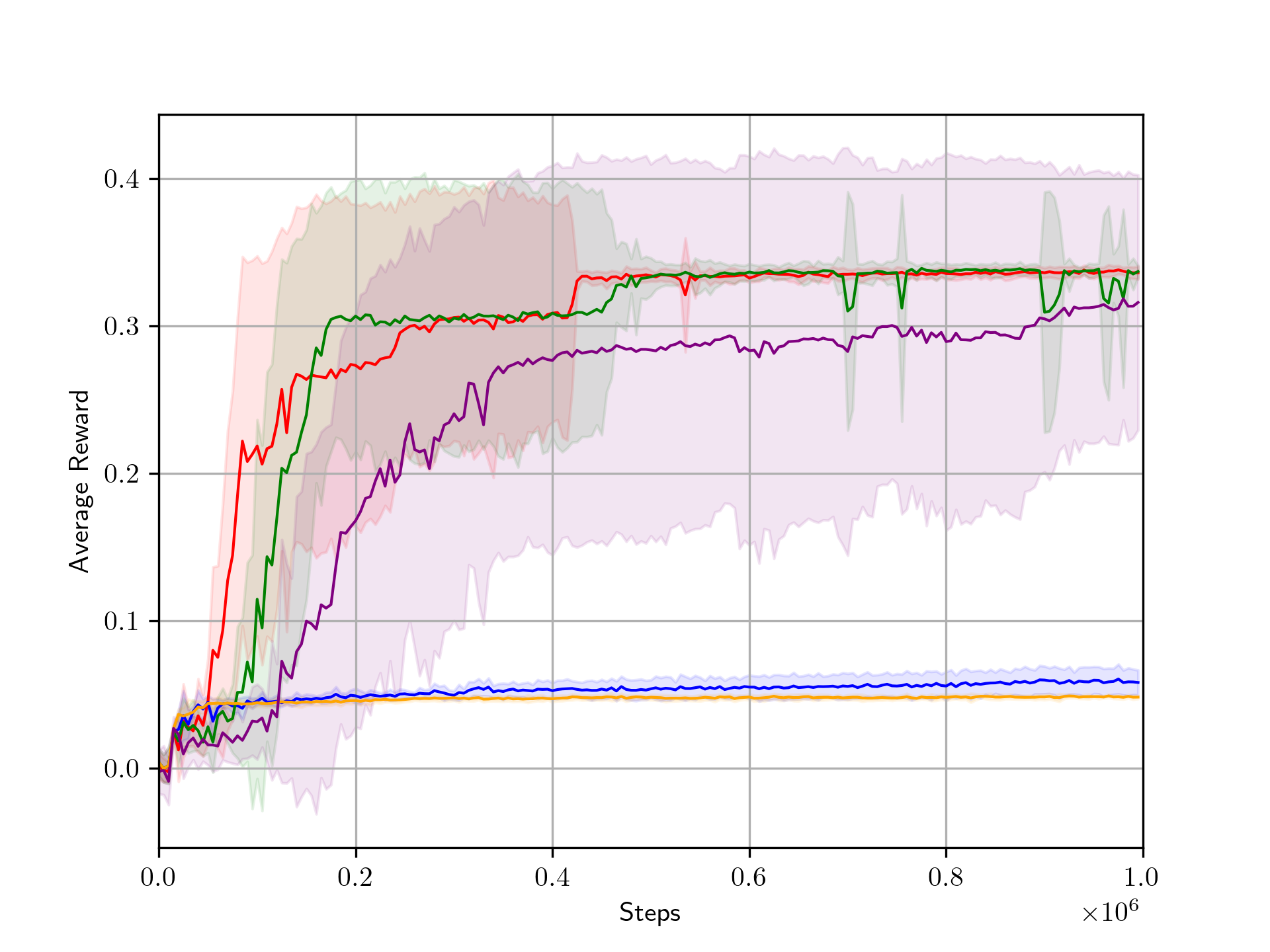
(a) Swimmer

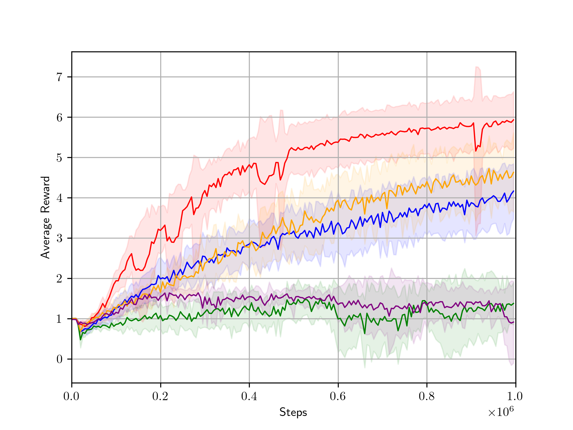
(b) Ant

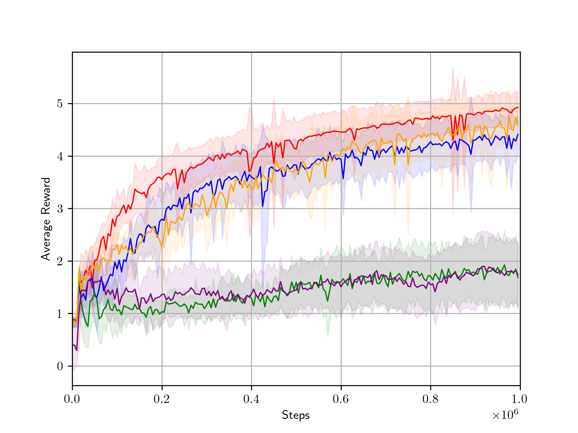
(c) Walker2d

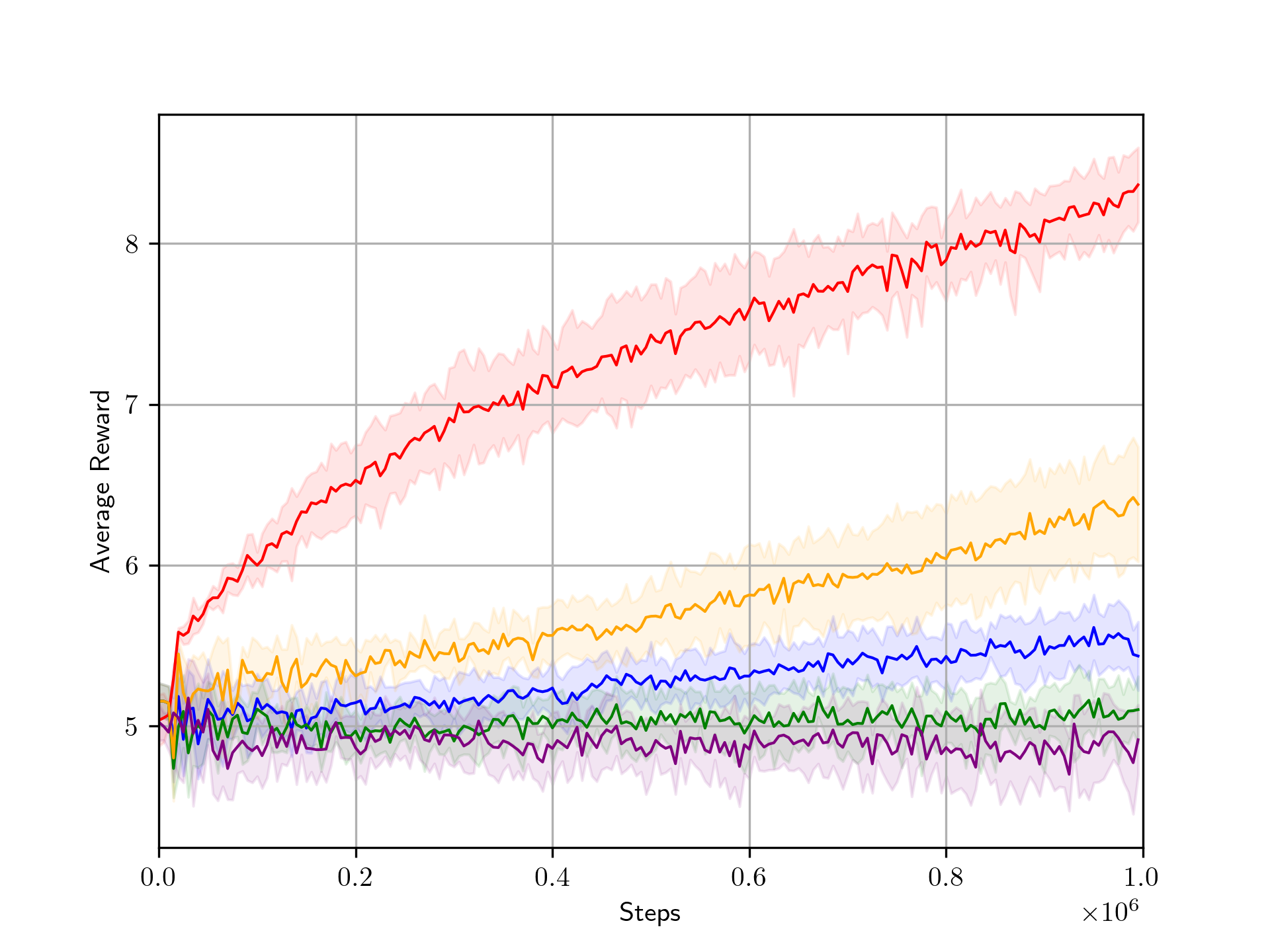
(d) Humanoid

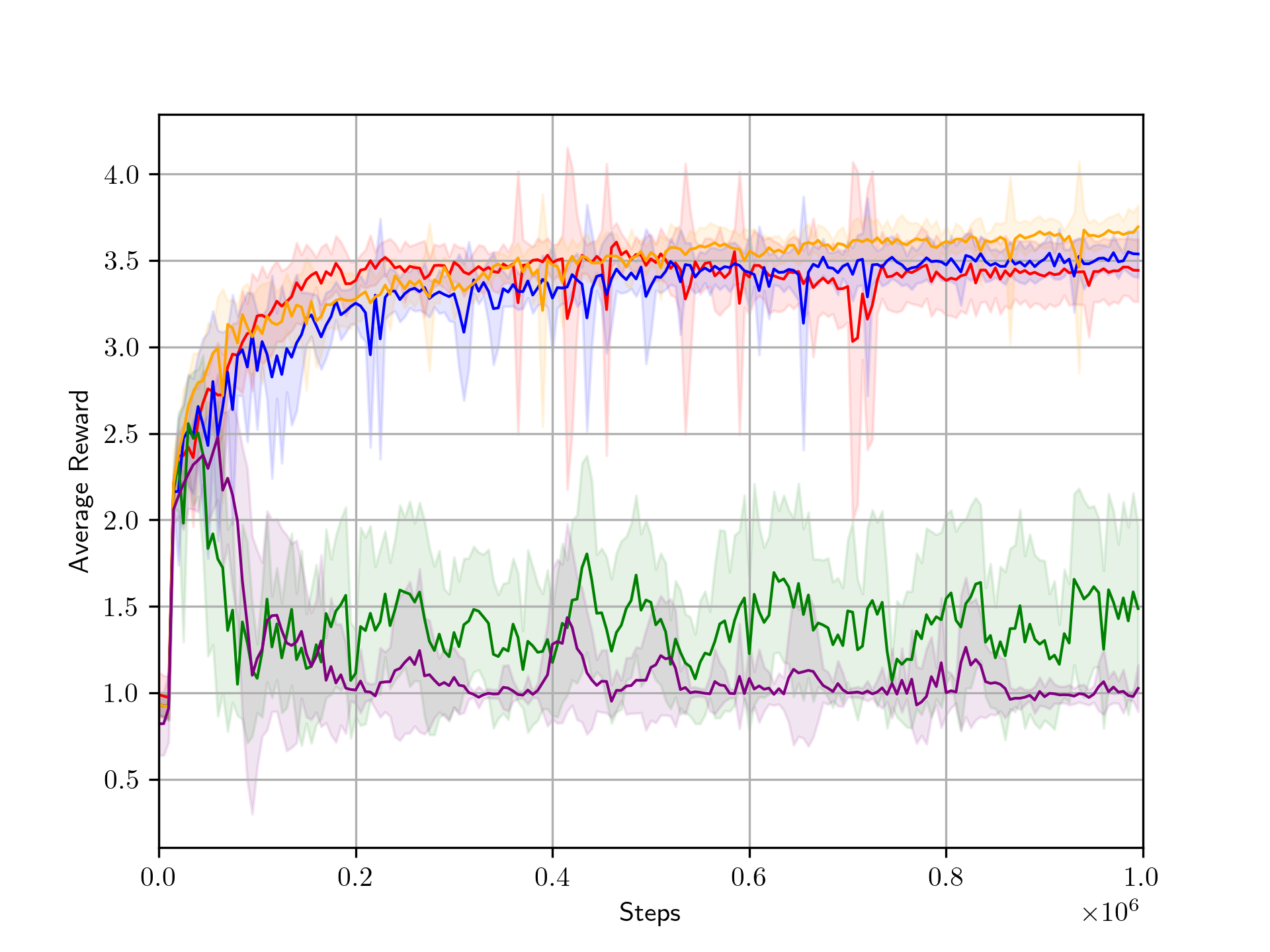
(e) Hopper

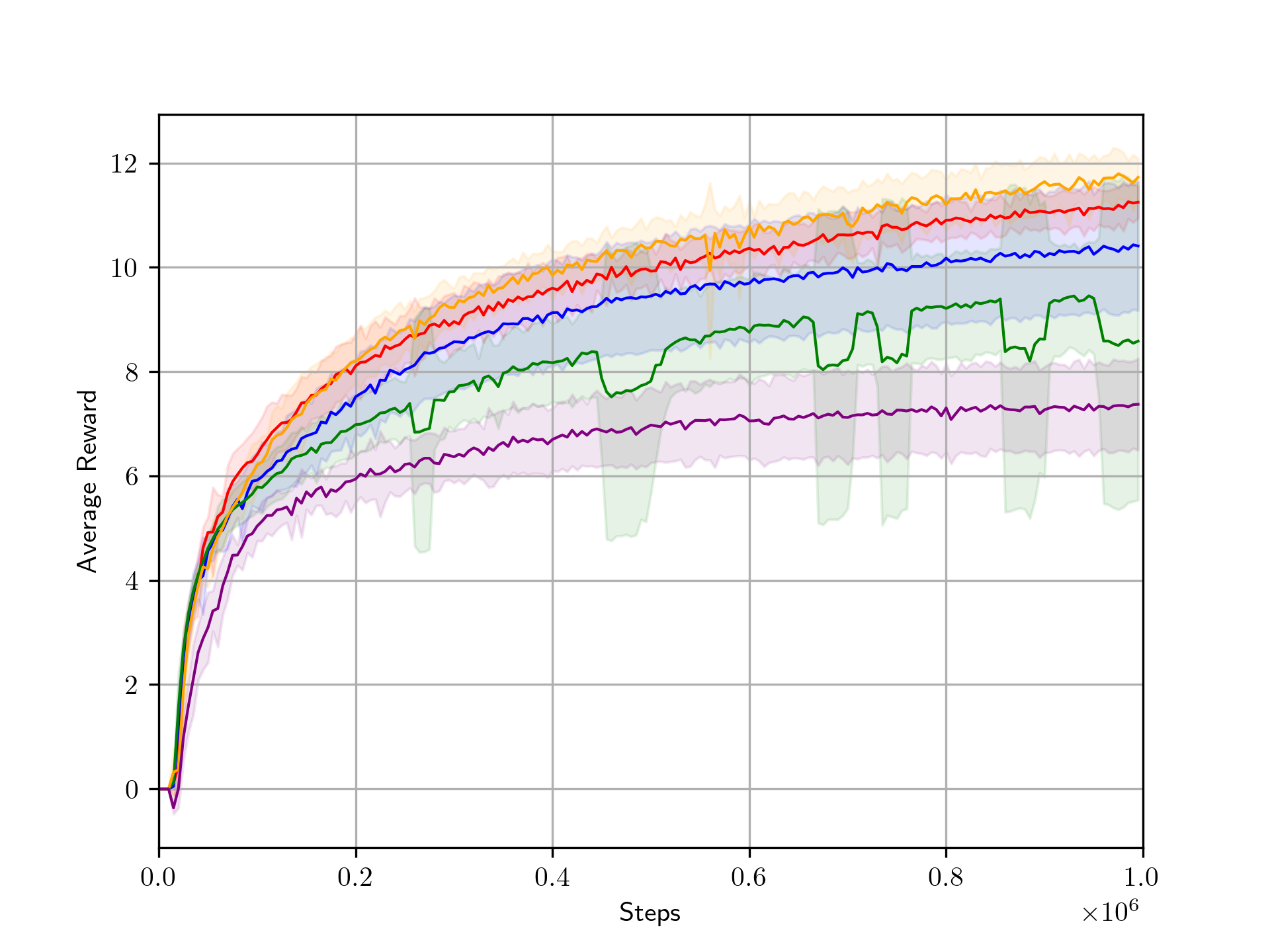
(f) HalfCheetah

Figure 3: Learning curves for the Gymnasium’s Mujoco tasks. The horizontal axis represents Steps, and the vertical axis represents the evaluation value (average reward). Lines and shades represent the mean and standard deviation of the evaluation values over 10 trials, respectively.

F.2 Perfomance Comparison with SAC and ARO-DDPG with Reset

Figure 4 presents the learning curves for all environments with termination (Ant, Hopper, Walker2d and Humanoid), similar to Figure 2(a) in Section 4.2, comparing RVI-SAC with SAC with automatic Reset Cost adjustment and ARO-DDPG with automatic Reset Cost adjustment. Here, the discount rate of SAC is set to $\gamma=0.99$. The results demonstrate that RVI-SAC outperforms SAC with automatic Reset Cost adjustment and ARO-DDPG with automatic Reset Cost adjustment across all environments.

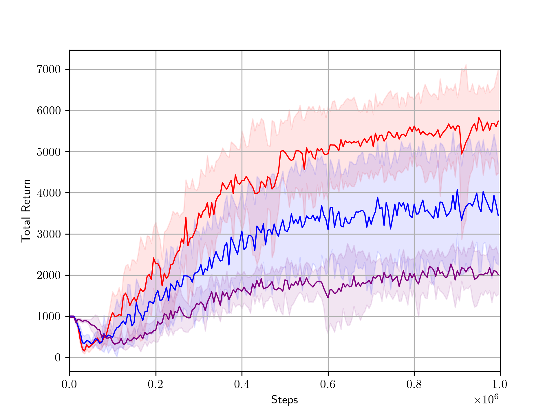
(a) Ant

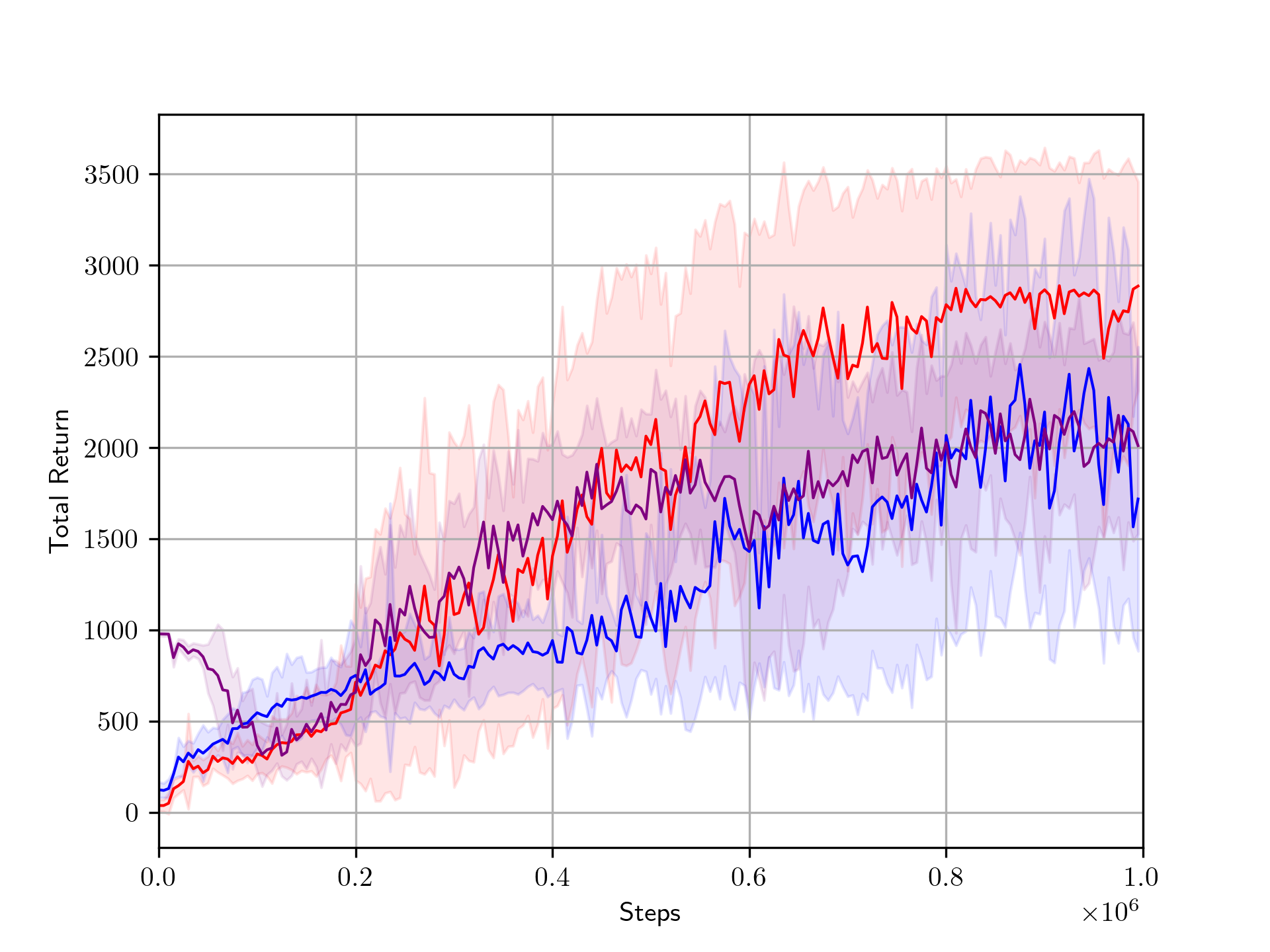
(b) Hopper

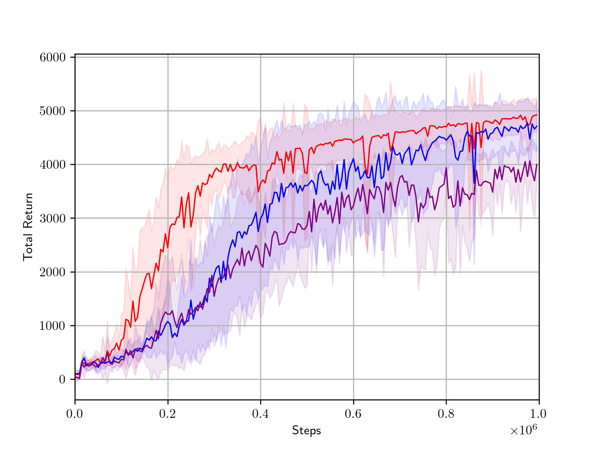
(c) Walker2d

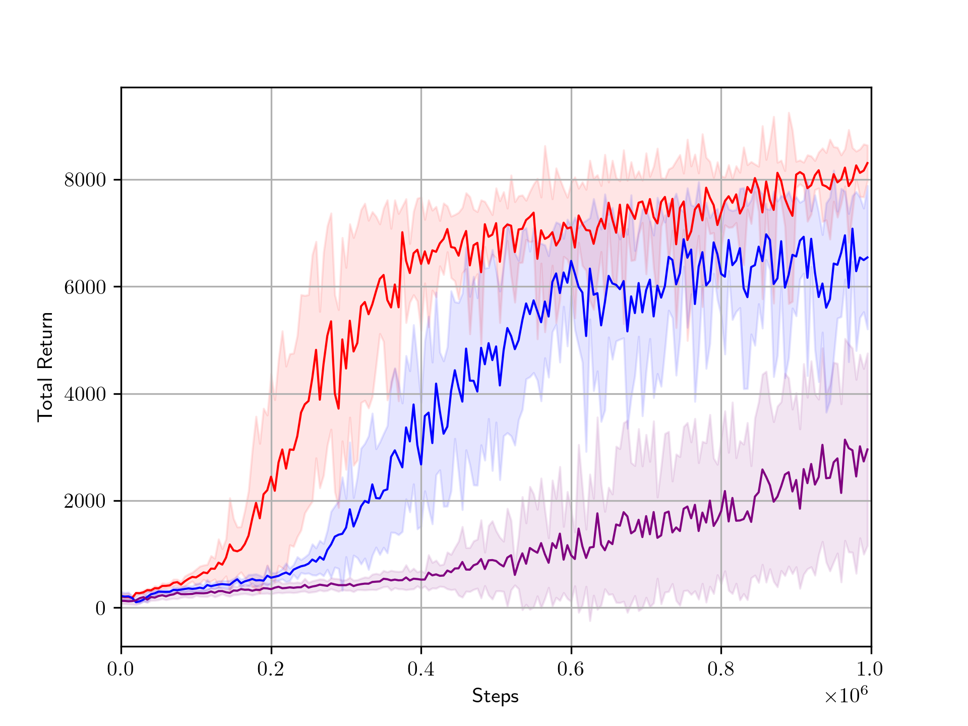
(d) Humanoid

Figure 4: This figure represent learning curves for all environments with termination, compare RVI-SAC (red) with SAC (blue) with automatic Reset Cost adjustment and ARO-DDPG(purple) with automatic Reset Cost adjustment.

References

- Abbasi-Yadkori et al. (2019) Abbasi-Yadkori, Y., Bartlett, P., Bhatia, K., Lazic, N., Szepesvari, C., and Weisz, G. POLITEX: Regret bounds for policy iteration using expert prediction. In Chaudhuri, K. and Salakhutdinov, R. (eds.), Proceedings of the 36th International Conference on Machine Learning, volume 97 of Proceedings of Machine Learning Research, pp. 3692–3702. PMLR, 09–15 Jun 2019. URL https://proceedings.mlr.press/v97/lazic19a.html.
- Abdolmaleki et al. (2018) Abdolmaleki, A., Springenberg, J. T., Tassa, Y., Munos, R., Heess, N., and Riedmiller, M. A. Maximum a posteriori policy optimisation. CoRR, abs/1806.06920, 2018. URL http://arxiv.org/abs/1806.06920.
- Abounadi et al. (2001) Abounadi, J., Bertsekas, D., and Borkar, V. S. Learning algorithms for markov decision processes with average cost. SIAM Journal on Control and Optimization, 40(3):681–698, 2001. doi: 10.1137/S0363012999361974. URL https://doi.org/10.1137/S0363012999361974.
- Blackwell (1962) Blackwell, D. Discrete dynamic programming. Annals of Mathematical Statistics, 33:719–726, 1962. URL https://api.semanticscholar.org/CorpusID:120274575.
- Borkar (1997) Borkar, V. S. Stochastic approximation with two time scales. Systems & Control Letters, 29(5):291–294, 1997. ISSN 0167-6911. doi: https://doi.org/10.1016/S0167-6911(97)90015-3. URL https://www.sciencedirect.com/science/article/pii/S0167691197900153.
- Borkar (2009) Borkar, V. S. Stochastic Approximation: A Dynamical Systems Viewpoint. Texts and Readings in Mathematics. Hindustan Book Agency Gurgaon, 1 edition, Jan 2009. ISBN 978-93-86279-38-5. doi: 10.1007/978-93-86279-38-5. URL https://doi.org/10.1007/978-93-86279-38-5. eBook Packages: Mathematics and Statistics, Mathematics and Statistics (R0).
- Dewanto & Gallagher (2021) Dewanto, V. and Gallagher, M. Examining average and discounted reward optimality criteria in reinforcement learning. CoRR, abs/2107.01348, 2021. URL https://arxiv.org/abs/2107.01348.
- Fujimoto et al. (2018) Fujimoto, S., van Hoof, H., and Meger, D. Addressing function approximation error in actor-critic methods. CoRR, abs/1802.09477, 2018. URL http://arxiv.org/abs/1802.09477.
- Gosavi (2004) Gosavi, A. Reinforcement learning for long-run average cost. European Journal of Operational Research, 155(3):654–674, 2004. ISSN 0377-2217. doi: https://doi.org/10.1016/S0377-2217(02)00874-3. URL https://www.sciencedirect.com/science/article/pii/S0377221702008743. Traffic and Transportation Systems Analysis.
- Haarnoja et al. (2017) Haarnoja, T., Tang, H., Abbeel, P., and Levine, S. Reinforcement learning with deep energy-based policies. CoRR, abs/1702.08165, 2017. URL http://arxiv.org/abs/1702.08165.
- Haarnoja et al. (2018a) Haarnoja, T., Zhou, A., Abbeel, P., and Levine, S. Soft actor-critic: Off-policy maximum entropy deep reinforcement learning with a stochastic actor, 2018a.
- Haarnoja et al. (2018b) Haarnoja, T., Zhou, A., Hartikainen, K., Tucker, G., Ha, S., Tan, J., Kumar, V., Zhu, H., Gupta, A., Abbeel, P., and Levine, S. Soft actor-critic algorithms and applications. CoRR, abs/1812.05905, 2018b. URL http://arxiv.org/abs/1812.05905.
- Konda & Borkar (1999) Konda, V. R. and Borkar, V. S. Actor-critic–type learning algorithms for markov decision processes. SIAM Journal on Control and Optimization, 38(1):94–123, 1999. doi: 10.1137/S036301299731669X. URL https://doi.org/10.1137/S036301299731669X.
- Lillicrap et al. (2019) Lillicrap, T. P., Hunt, J. J., Pritzel, A., Heess, N., Erez, T., Tassa, Y., Silver, D., and Wierstra, D. Continuous control with deep reinforcement learning, 2019.
- Ma et al. (2021) Ma, X., Tang, X., Xia, L., Yang, J., and Zhao, Q. Average-reward reinforcement learning with trust region methods. CoRR, abs/2106.03442, 2021. URL https://arxiv.org/abs/2106.03442.
- Mnih et al. (2013) Mnih, V., Kavukcuoglu, K., Silver, D., Graves, A., Antonoglou, I., Wierstra, D., and Riedmiller, M. A. Playing atari with deep reinforcement learning. CoRR, abs/1312.5602, 2013. URL http://arxiv.org/abs/1312.5602.
- Mnih et al. (2016) Mnih, V., Badia, A. P., Mirza, M., Graves, A., Lillicrap, T., Harley, T., Silver, D., and Kavukcuoglu, K. Asynchronous methods for deep reinforcement learning. In Balcan, M. F. and Weinberger, K. Q. (eds.), Proceedings of The 33rd International Conference on Machine Learning, volume 48 of Proceedings of Machine Learning Research, pp. 1928–1937, New York, New York, USA, 20–22 Jun 2016. PMLR. URL https://proceedings.mlr.press/v48/mniha16.html.
- Naik et al. (2019) Naik, A., Shariff, R., Yasui, N., and Sutton, R. S. Discounted reinforcement learning is not an optimization problem. CoRR, abs/1910.02140, 2019. URL http://arxiv.org/abs/1910.02140.
- Puterman (1994) Puterman, M. L. Markov Decision Processes: Discrete Stochastic Dynamic Programming. John Wiley & Sons, Inc., USA, 1st edition, 1994. ISBN 0471619779.
- Saxena et al. (2023) Saxena, N., Khastigir, S., Kolathaya, S., and Bhatnagar, S. Off-policy average reward actor-critic with deterministic policy search, 2023.
- Schulman et al. (2015) Schulman, J., Levine, S., Moritz, P., Jordan, M. I., and Abbeel, P. Trust region policy optimization. CoRR, abs/1502.05477, 2015. URL http://arxiv.org/abs/1502.05477.
- Schulman et al. (2017) Schulman, J., Wolski, F., Dhariwal, P., Radford, A., and Klimov, O. Proximal policy optimization algorithms. CoRR, abs/1707.06347, 2017. URL http://arxiv.org/abs/1707.06347.
- Schwartz (1993) Schwartz, A. A reinforcement learning method for maximizing undiscounted rewards. In Utgoff, P. E. (ed.), Machine Learning, Proceedings of the Tenth International Conference, University of Massachusetts, Amherst, MA, USA, June 27-29, 1993, pp. 298–305. Morgan Kaufmann, 1993. doi: 10.1016/B978-1-55860-307-3.50045-9. URL https://doi.org/10.1016/b978-1-55860-307-3.50045-9.
- Silver et al. (2014) Silver, D., Lever, G., Heess, N., Degris, T., Wierstra, D., and Riedmiller, M. Deterministic policy gradient algorithms. In Xing, E. P. and Jebara, T. (eds.), Proceedings of the 31st International Conference on Machine Learning, volume 32 of Proceedings of Machine Learning Research, pp. 387–395, Bejing, China, 22–24 Jun 2014. PMLR. URL https://proceedings.mlr.press/v32/silver14.html.
- Singh (1994) Singh, S. Reinforcement learning algorithms for average-payoff markovian decision processes. In AAAI Conference on Artificial Intelligence, 1994. URL https://api.semanticscholar.org/CorpusID:17854729.
- Sutton & Barto (2018) Sutton, R. S. and Barto, A. G. Reinforcement Learning: An Introduction. The MIT Press, second edition, 2018. URL http://incompleteideas.net/book/the-book-2nd.html.
- Todorov et al. (2012) Todorov, E., Erez, T., and Tassa, Y. Mujoco: A physics engine for model-based control. In 2012 IEEE/RSJ International Conference on Intelligent Robots and Systems, pp. 5026–5033, Vilamoura-Algarve, Portugal, 2012. doi: 10.1109/IROS.2012.6386109.
- Towers et al. (2023) Towers, M., Terry, J. K., Kwiatkowski, A., Balis, J. U., Cola, G. d., Deleu, T., Goulão, M., Kallinteris, A., KG, A., Krimmel, M., Perez-Vicente, R., Pierré, A., Schulhoff, S., Tai, J. J., Shen, A. T. J., and Younis, O. G. Gymnasium, March 2023. URL https://zenodo.org/record/8127025.
- Tsitsiklis (1994) Tsitsiklis, J. N. Asynchronous stochastic approximation and q-learning. Machine Learning, 16(3):185–202, 9 1994. doi: 10.1023/A:1022689125041. URL https://doi.org/10.1023/A:1022689125041.
- Wan & Sutton (2022) Wan, Y. and Sutton, R. S. On convergence of average-reward off-policy control algorithms in weakly communicating mdps, 2022.
- Wan et al. (2020) Wan, Y., Naik, A., and Sutton, R. S. Learning and planning in average-reward markov decision processes. CoRR, abs/2006.16318, 2020. URL https://arxiv.org/abs/2006.16318.
- Yang et al. (2016) Yang, S., Gao, Y., An, B., Wang, H., and Chen, X. Efficient average reward reinforcement learning using constant shifting values. Proceedings of the AAAI Conference on Artificial Intelligence, 30(1), Mar. 2016. doi: 10.1609/aaai.v30i1.10285. URL https://ojs.aaai.org/index.php/AAAI/article/view/10285.
- Zhang et al. (2021a) Zhang, S., Wan, Y., Sutton, R. S., and Whiteson, S. Average-reward off-policy policy evaluation with function approximation. CoRR, abs/2101.02808, 2021a. URL https://arxiv.org/abs/2101.02808.
- Zhang et al. (2021b) Zhang, S., Yao, H., and Whiteson, S. Breaking the deadly triad with a target network. In Meila, M. and Zhang, T. (eds.), Proceedings of the 38th International Conference on Machine Learning, volume 139 of Proceedings of Machine Learning Research, pp. 12621–12631. PMLR, 18–24 Jul 2021b. URL https://proceedings.mlr.press/v139/zhang21y.html.
- Zhang & Ross (2021) Zhang, Y. and Ross, K. W. On-policy deep reinforcement learning for the average-reward criterion. CoRR, abs/2106.07329, 2021. URL https://arxiv.org/abs/2106.07329.