Restriction of Schrödinger eigenfunctions to submanifolds

Abstract.

Burq-Gérard-Tzvetkov [15] and Hu [34] established $L^{p}$ estimates for the restriction of Laplace-Beltrami eigenfunctions to submanifolds. We investigate the eigenfunctions of the Schrödinger operators with critically singular potentials, and estimate the $L^{p}$ norms and period integrals for their restriction to submanifolds. Recently, Blair-Sire-Sogge [6] obtained global $L^{p}$ bounds for Schrödinger eigenfunctions by the resolvent method. Due to the Sobolev trace inequalities, the resolvent method cannot work for submanifolds of all dimensions. We get around this difficulty and establish spectral projection bounds by the wave kernel techniques and the bootstrap argument involving an induction on the dimensions of the submanifolds.

1. Introduction

Let $n\geq 2$. Let $(M,g)$ be a compact smooth $n$-dimensional Riemannian manifold (without boundary) and let $\Delta_{g}$ be the associated Laplace-Beltrami operator. It is known that the spectrum of $-\Delta_{g}$ is discrete and nonnegative (see e.g. [51]). Let $e_{\lambda}$ denote the $L^{2}$-normalized eigenfunction

$$-\Delta_{g}e_{\lambda}=\lambda^{2}e_{\lambda},\quad\text{and }\,\,\int_{M}|e_{\lambda}(x)|^{2}\,dx=1.$$

so that $\lambda\geq 0$ is the eigenvalue of the operator $\sqrt{-\Delta_{g}}.$

One of the main topics on eigenfunctions is to measure possible concentrations. There are several popular ways to do this.

1. The first way is by describing semi-classical (Wigner) measures, see the works by Shnirelman [47], Zelditch [63], Colin de Verdière [23], Gérard-Leichtnam [25], Zelditch-Zworski [65], Helffer-Martinez-Robert [31], Sarnak [45], Lindenstrauss [42] and Anantharaman [1].

2. The second way is by estimating the growth of the $L^{p}$ norms of eigenfunctions, see the works by Sogge [49, 50], Sogge-Zelditch [55], Burq-Gérard-Tzvetkov [17, 16, 18], Koch-Tataru [41], Hassell-Tacy [30], Hazari-Rivière [32], Blair-Sogge [11], Blair-Huang-Sogge [3], Huang-Sogge [36].

3. The third way is by measuring the growth of the $L^{p}$ norms over some local domains, specifically, geodesic balls or tubes along geodesics, see the works by Sogge [52, 53], Blair-Sogge [7, 8, 9, 10], Han [29], Hezari-Riviére [32], Wang-Zhang [59].

4. The fourth way is by studying the possible growth of $L^{p}$ norms and period integrals of eigenfunctions restricted to submanifolds, see the works by Burq-Gérard-Tzvetkov [15], Hu [34], Bourgain [12], Reznikov [43, 44], Tacy [56], Bourgain-Rudnick [13], Chen [21], Chen-Sogge [22], Xi-Zhang [62], Wang-Zhang [58], Hezari [33], Blair [2], Zhang [66], Huang-Zhang [37], Zelditch [64], Sogge-Xi-Zhang [54], Canzani-Galkowski-Toth [19], Canzani-Galkowski [20], Wyman [60, 61].

In this paper, we investigate the concentration of eigenfunctions in the fourth way.

1.1. Schrödinger eigenfunctions

We consider the Schrödinger operators

$$H_{V}=-\Delta_{g}+V$$

with singular potentials $V$ on the compact manifold $(M,g)$. We shall assume throughout that the potentials $V$ are real-valued and $V\in\mathcal{K}(M)$, which is the Kato class. It is all $V\in L^{1}(M)$ satisfying

$$\lim_{\delta\to 0}\sup_{x\in M}\int_{d_{g}(y,x)<\delta}|V(y)|W_{n}(d_{g}(x,y))dy=0,$$

where

$$W_{n}(r)=\begin{cases}r^{2-n},\quad\quad\quad\quad n\geq 3\\ \log(2+r^{-1}),\ \ n=2\end{cases}$$

and $d_{g}$, $dy$ denote geodesic distance, the volume element on $(M,g)$. Note that by Hölder inequality, we have $L^{q}\subset\mathcal{K}(M)\subset L^{1}(M)$ for all $q>\frac{n}{2}$. The Kato class $\mathcal{K}(M)$ and $L^{n/2}(M)$ share the same critical scaling behavior, while neither one is contained in the other one for $n\geq 3$. For instance, singularities of the type $|x|^{-\alpha}$ for $\alpha<2$ are allowed for both classes. These singular potentials appear naturally in physics, most notably the Coulomb potential $|x|^{-1}$ in three dimensions. See the survey paper [48] by Barry Simon for a detailed introduction to the Kato potentials and their physical motivations.

The Kato class is the “minimal condition” to ensure that $H_{V}$ is essentially self-adjoint and bounded from below, and eigenfunctions of $H_{V}$ are bounded. Since $M$ is compact, the spectrum of $H_{V}$ is discrete. Also, the associated eigenfunctions are continuous. The following Gaussian heat kernel bounds holds for $x,y\in M$

(1.1) $$|e^{-tH_{V}}(x,y)|\lesssim t^{-\frac{n}{2}}e^{-cd_{g}(x,y)^{2}/t},\ 0<t\leq 1.$$

See e.g. Blair-Sire-Sogge [6], Simon [48] and references therein for the detailed introduction. After possibly adding a constant to $V$ we may assume throughout that $H_{V}$ is bounded below by one, i.e.,

(1.2) $$\|f\|_{2}^{2}\leq\langle\,H_{V}f,\,f\,\rangle,\quad f\in\text{Dom }(H_{V}).$$

We shall write the spectrum of $\sqrt{H_{V}}$ as

(1.3) $$\{\tau_{k}\}_{k=1}^{\infty},$$

where the eigenvalues are arranged in increasing order and we account for multiplicity. For each $\tau_{k}$ there is an eigenfunction $e_{\tau_{k}}\in\text{Dom }(H_{V})$ (the domain of $H_{V}$) so that

(1.4) $$H_{V}e_{\tau_{k}}=\tau^{2}_{k}e_{\tau_{k}},\ \ {\rm and}\ \ \int_{M}|e_{\tau_{k}}(x)|^{2}\,dx=1.$$

Moreover, we shall let

(1.5) $$H^{0}=-\Delta_{g}$$

be the unperturbed operator. The corresponding eigenvalues and associated $L^{2}$-normalized eigenfunctions are denoted by $\{\lambda_{j}\}_{j=1}^{\infty}$ and $\{e^{0}_{j}\}_{j=1}^{\infty}$, respectively so that

(1.6) $$H^{0}e^{0}_{j}=\lambda^{2}_{j}e^{0}_{j},\quad\text{and }\,\,\int_{M}|e^{0}_{j}(x)|^{2}\,dx=1.$$

Both $\{e_{\tau_{k}}\}_{k=1}^{\infty}$ and $\{e^{0}_{j}\}_{j=1}^{\infty}$ are orthonormal bases for $L^{2}(M)$. Let $P^{0}=\sqrt{H^{0}}$ and $P_{V}=\sqrt{H_{V}}$. Let ${\rm 1\rule{0.43057pt}{6.54443pt}\hskip 0.86108pt}_{\lambda}(\tau)$ be the indicator function of the interval $[\lambda-1,\lambda+1]$. We define the unit-band spectral projection operators ${\rm 1\rule{0.43057pt}{6.54443pt}\hskip 0.86108pt}_{\lambda}(P^{0})$ and ${\rm 1\rule{0.43057pt}{6.54443pt}\hskip 0.86108pt}_{\lambda}(P_{V})$ by the spectral theorem.

1.2. Eigenfunction restriction estimates

We first review the previous results.

Blair-Sire-Sogge [6] and Blair-Huang-Sire-Sogge [4] established the following $L^{p}$ estimates for the unit-band spectral projection operator ${\rm 1\rule{0.43057pt}{6.54443pt}\hskip 0.86108pt}_{\lambda}(P_{V})$, which extend Sogge’s seminal work [49] to Schrödinger operators with critically singular potentials.

Theorem 1.1.

Let $M$ be a compact manifold of dimension $n\geq 2$. Let $q_{c}=\frac{2n+2}{n-1}$. If $V\in\mathcal{K}(M)\cap L^{n/2}(M)$, then we have for some constant $C_{V}$ independent of $\lambda$

(1.7) $$\|{\rm 1\rule{0.43057pt}{6.54443pt}\hskip 0.86108pt}_{\lambda}(P_{V})\|_{L^{2}(M)\to L^{p}(M)}\leq C_{V}\lambda^{\sigma(p)},$$

where Sogge’s exponent

$$\sigma(p)=\begin{cases}\frac{n-1}{2}-\frac{n}{p},\ \ \ \ \ \ \ q_{c}\leq p\leq\infty\\ \frac{n-1}{2}(\frac{1}{2}-\frac{1}{p}),\ \ \ \ 2\leq p<q_{c}.\end{cases}$$

Moreover, if we only assume that $V\in L^{n/2}(M)$ when $n\geq 3$, then (1.7) still holds for $2\leq p\leq\frac{2n}{n-4}$ when $n\geq 5$ and $2\leq p<\infty$ when $n=3,4$.

These estimates are sharp on any compact manifolds when $V\equiv 0$ and improve the Sobolev estimates. Indeed, they are saturated on the sphere $S^{n}$ by Zonal functions when $p\geq q_{c}$, and by Gaussian beams when $p\leq q_{c}$.

Next, Burq-Gérard-Tzvetkov [15] and Hu [34] obtained the $L^{p}$ restriction estimates of the unit-band spectral projection operator ${\rm 1\rule{0.43057pt}{6.54443pt}\hskip 0.86108pt}_{\lambda}(P^{0})$, which implies the $L^{p}$ estimates for the eigenfunctions restricted to submanifolds. See also the works by Greenleaf-Seeger [28], Tataru [57], Reznikov [43] for earlier related results.

Theorem 1.2.

Let $M$ be a compact manifold of dimension $n\geq 2$. Let $\Sigma$ be a submanifold of dimension $1\leq k\leq n-1$. Then we have for $2\leq p\leq\infty$

(1.8) $$\|{\rm 1\rule{0.43057pt}{6.54443pt}\hskip 0.86108pt}_{\lambda}(P^{0})\|_{L^{2}(M)\to L^{p}(\Sigma)}\leq CA,$$

where $C$ is a constant independent of $\lambda$, and

• If $k\leq n-3$, then $A=\lambda^{\frac{n-1}{2}-\frac{k}{p}}$ for $2\leq p\leq\infty$.

• If $k=n-2$, then $A=\lambda^{\frac{n-1}{2}-\frac{k}{p}}$ for $2<p\leq\infty$, and $A=\lambda^{\frac{1}{2}}(\log\lambda)^{\frac{1}{2}}$ for $p=2$.

• If $k=n-1$, then $A=\lambda^{\frac{n-1}{2}-\frac{k}{p}}$ for $\frac{2n}{n-1}\leq p\leq\infty$, and $A=\lambda^{\frac{n-1}{4}-\frac{n-2}{2p}}$ for $2\leq p<\frac{2n}{n-1}$.

In the theorem, the bound $A$ has the explicit form $\lambda^{\delta(p)}(\log\lambda)^{\theta}$, and depends on $\lambda,\ k,\ n,\ p$. We simply use the short notation $A$ in many cases where we do not need its explicit form and the parameters are fixed. In the following, we denote the endpoints $p_{c}=\frac{2n}{n-1}$ when $k=n-1$ and $p_{c}=2$ when $k\leq n-2$. Note that $p=2$ is also a special endpoint when $k=n-1$, and we shall handle it independently in our proof. When $k=n-1$, if $\Sigma$ has non-vanishing Gaussian curvature, then there is a power improvement: $A=\lambda^{\frac{n-1}{3}-\frac{2n-3}{3p}}$ for $2\leq p<\frac{2n}{n-1}$. It was proved by Burq-Gérard-Tzvetkov [15] $(n=2)$ and Hu [34] $(n\geq 3)$.

These estimates are essentially sharp and they improve the Sobolev trace inequalities. Indeed, they are saturated on the sphere $S^{n}$ by Zonal functions when $p\geq p_{c}$, and by Gaussian beams when $p\leq p_{c}$.

Remark 1.3.

There was a log loss at the endpoint $p_{c}=\frac{2n}{n-1}$ when $k=n-1$ in [15], but later Hu [34] removed this log loss by applying the oscillatory integral theorems of Greenleaf-Seeger [28]. The log loss at the endpoint $p_{c}=2$ when $k=n-2$ is more subtle, and it was only conditionally removed by Chen-Sogge [22] and Wang-Zhang [58]. It has long been believed that the log loss can be removed in general, but this problem is still open (see [58]).

1.3. Main results

Inspired by the previous works, we prove the following $L^{p}$ restriction estimates of the unit-band spectral projection operator ${\rm 1\rule{0.43057pt}{6.54443pt}\hskip 0.86108pt}_{\lambda}(P_{V})$. The Kato class ensures that the Schrödinger eigenfunctions are continuous so that their restriction on submanifolds makes sense. These results cover Theorem 1.2.

Theorem 1.4.

Let $M$ be a compact manifold of dimension $n\geq 2$. Let $\Sigma$ be a submanifold of dimension $k$. If $V\in\mathcal{K}(M)\cap L^{n/2}(M)$, then we have

(1.9) $$\|{\rm 1\rule{0.43057pt}{6.54443pt}\hskip 0.86108pt}_{\lambda}(P_{V})\|_{L^{2}(M)\to L^{p}(\Sigma)}\leq C_{V}A,\ \ 2\leq p\leq\infty,$$

for $k\leq n/2$ when $n\geq 5$ and for all $k$ when $n\leq 4$. In the case $k>n/2$ when $n\geq 5$, there exist $q_{k}\geq 2$ and $0<\theta_{k,p}\leq 1$ such that

(1.10) $$\|{\rm 1\rule{0.43057pt}{6.54443pt}\hskip 0.86108pt}_{\lambda}(P_{V})\|_{L^{2}(M)\to L^{p}(\Sigma)}\leq\begin{cases}C_{V}A(\log\lambda)^{\theta_{k,p}},\ \ 2\leq p\leq q_{k},\\ C_{V}A,\ \ \ \ \ \ \ \ \ \ \ \ \ q_{k}<p\leq\infty.\end{cases}$$

Moreover, if $V\in L^{q}(M)$ with $q>n/2$, then we have (1.9) for all $n$ and $k$. Here $A$ is defined in (1.8) and $C_{V}$ is a constant independent of $\lambda$.

As a corollary, this theorem implies the $L^{p}$ estimates for the Schrödinger eigenfunctions restricted to submanifolds.

Remark 1.5.

In the proof, we obtain

$$q_{n-1}=\begin{cases}45/22\approx 2.045,\ \ \ \ \ n=5\\ 168/79\approx 2.127,\ \ \ \ n=6\\ 280/127\approx 2.205,\ \ \ n=7\\ 9/4=2.250,\ \ \ \ \ \ \ \ \ n=8\\ \frac{2n(-2+n+3n^{2})}{16+4n-3n^{2}+3n^{3}}=2+\frac{8}{3n}-\frac{4}{3n^{2}}+O(\frac{1}{n^{3}}),\ \ n\geq 9\end{cases}$$

and when $k\in(n/2,n-2]$,

$$q_{k}=\frac{2kn(n+1)}{k(n^{2}-n-4)+n^{2}+3n}=2+\frac{2(k+1)}{n^{2}}+O(\frac{1}{n^{3}}).$$

Here $q_{k}$ is increasing in $k$, and $q_{n-1}<p_{c}$ when $n\leq 8$. Moreover, $\theta_{k,p}=1$ for $p=2$ and $p=p_{c}$ (if $q_{k}\geq p_{c}$), while others follow from interpolation. See Section 3.1.

Remark 1.6.

If $k=n-1$ and $\Sigma$ has non-vanishing Gaussian curvature, we can establish a similar theorem with $A$ replaced by $\lambda^{\frac{n-1}{3}-\frac{2n-3}{3p}}$ when $2\leq p<\frac{2n}{n-1}$. Indeed, if we assume that $V\in\mathcal{K}(M)\cap L^{n/2}(M)$, then (1.9) holds when $n=2,3$. When $n\geq 4$, there exist $q_{n-1}\geq 2$ and $0<\theta_{n-1,p}\leq 1$ such that (1.10) holds. Moreover, if $V\in L^{q}(M)$ with $q>n/2$, then we have (1.9) for all $n$. The proof is essentially the same, but the values of $q_{n-1}$ are slightly different. See Section 3.1.

In the proof of Theorem 1.4, we use a perturbation argument based on Duhamel’s principle and split the frequency into two parts. In the high-frequency regime, the classical resolvent method (see e.g. [6], [4]) can only handle codimension $1$ and $2$ due to the Sobolev trace inequalities. We get around this difficulty by using the wave kernel techniques to handle the spectral projection operators directly. The novelty of our argument here is a bootstrap argument involving an induction on the dimensions of the submanifolds. See Section 2 for details.

For the low-frequency regime, we need to prove for some $\frac{1}{p_{0}}\in[\frac{n+3}{2n+2}-\frac{2}{n},\frac{n-1}{2n+2}]$

(1.11) $$\|(-\Delta_{g}-\lambda^{2}+i\lambda)^{-1}\psi(P^{0}/\lambda)\|_{L^{p_{0}^{\prime}}(M)\to L^{p_{c}}(\Sigma)}\lesssim A\lambda^{\sigma(p_{0})-1}.$$

Here $\psi\in C_{0}^{\infty}(\mathbb{R})$ satisfies $\psi(t)=1$ if $|t|\leq 2$ and $\psi(t)=0$ if $|t|>3$. By (1.7) and (1.8), it is straightforward to use a duality argument to obtain (1.11) with a log loss, but the difficulty is to remove this loss. We further reduce it to estimating the norm of the oscillatory integral operator

$$T^{\lambda}f(x)=\int_{M}e^{i\lambda d_{g}(x,y)}a(x,y)f(y)dy$$

where $a(x,y)$ is supported in $\{d_{g}(x,y)\in(1/4,4)\}$ and $|\partial_{x,y}^{\gamma}a(x,y)|\leq C_{\gamma}.$ We will have (1.11) if there is a $\delta_{0}>0$ such that

(1.12) $$\|T^{\lambda}\|_{L^{p_{0}^{\prime}}(M)\to L^{p_{c}}(\Sigma)}\lesssim\lambda^{\frac{n-1}{2}-\frac{n}{p_{0}}-\frac{k}{p_{c}}-\delta_{0}}.$$

In Section 3, we can establish (1.12) for $k\leq n/2$ when $n\geq 5$ and for all $k$ when $n\leq 4$. We shall further discuss the bounds of this oscillatory integral operator in Section 5.

Furthermore, by the same method, we can also obtain period integral estimates for Schrödinger eigenfunctions. These extend the previous results for the Laplacian eigenfunctions by Good [26], Hejhal [27], Zelditch [64], Reznikov [44].

Theorem 1.7.

Let $M$ be a compact manifold of dimension $n\geq 2$. Let $\Sigma$ be a submanifold of dimension $k$. Let $V\in\mathcal{K}(M)\cap L^{n/2}(M)$. If $H_{V}e_{\lambda}=\lambda^{2}e_{\lambda}$ with $\lambda>1$, then we have

(1.13) $$\Big{|}\int_{\Sigma}e_{\lambda}d\sigma\Big{|}\leq C_{V}\lambda^{\frac{n-k-1}{2}}$$

for $k\leq n/2$ and $k\geq n-3$ when $n\geq 9$ and for all $k$ when $n\leq 8$. In the case $n/2<k\leq n-4$ when $n\geq 9$, we have

(1.14) $$\Big{|}\int_{\Sigma}e_{\lambda}d\sigma\Big{|}\leq C_{V}\lambda^{\frac{n-k-1}{2}}\log\lambda.$$

Moreover, if $V\in L^{q}(M)$ with $q>n/2$, then we have (1.13) for all $n$ and $k$. Here $\sigma$ is the volume measure on $\Sigma$ induced by the Riemannian metric, and $C_{V}$ is a constant independent of $\lambda$.

As before, one may expect to remove the log loss for all $n$ and $k$ under the critical condition that $V\in\mathcal{K}(M)\cap L^{n/2}(M)$. Since the $L^{2}$ restriction bound $A=\lambda^{\frac{n-k-1}{2}}$ when $n/2<k\leq n-4$, it suffices to removed the log loss for the $L^{2}$ bounds in (1.10). Moreover, it is worth mentioning that our method can still be used to obtain improvements on negatively curved manifolds and extend the results by Chen-Sogge [22], Sogge-Xi-Zhang [54], Canzani-Galkowski-Toth [19], Canzani-Galkowski [20], Wyman [60, 61].

Remark 1.8.

In a recent work by Blair-Park [5], they used the resolvent method (see e.g. [6], [4]) to obtain Schrödinger quasimode estimates in the cases $k=n-1,n-2$ for certain ranges of $p$. Even in these two cases, we can get larger ranges of $p$, since we do not require the “uniform resolvent conditions” (see Remark 3.2). Furthermore, Blair-Park [5] also considered the improvements on non-positively curved manifolds. Our method can be used to obtain these improvements as well by considering the spectral projections on shrinking intervals. In this paper, we only focus on the unit-band spectral projections for simplicity.

1.4. Paper structure

The paper is structured as follows. In Section 2, we presents the main argument for the proof of Theorem 1.4. The proof consists of several cases. In Section 3, we remove the log loss in Case 2. In Section 4, we consider period integrals and prove Theorem 1.7. In Section 5, we further discuss the bounds of the oscillatory integral operator.

1.5. Notations

Throughout this paper, $X\lesssim Y$ means $X\leq CY$ for some positive constants $C$. If $X\lesssim Y$ and $Y\lesssim X$, we denote $X\approx Y$. If $x$ is in a small neighborhood of $x_{0}$, we denote $x\sim x_{0}$. Let ${\rm 1\rule{0.43057pt}{6.54443pt}\hskip 0.86108pt}_{\lambda}={\rm 1\rule{0.43057pt}{6.54443pt}\hskip 0.86108pt}_{[\lambda-1,\lambda+1]}$, ${\rm 1\rule{0.43057pt}{6.54443pt}\hskip 0.86108pt}_{\lambda,\ell}(s)={\rm 1\rule{0.43057pt}{6.54443pt}\hskip 0.86108pt}_{|s-\lambda|\in(2^{\ell},2^{\ell+1}]}(s)$, ${\rm 1\rule{0.43057pt}{6.54443pt}\hskip 0.86108pt}_{\leq 2\lambda}={\rm 1\rule{0.43057pt}{6.54443pt}\hskip 0.86108pt}_{(-\infty,2\lambda]}$.

2. Main argument

We mainly focus on the endpoint estimates at $p=p_{c}$, as one can easily obtain other estimates by the same argument or by interpolation. Note that $p=2$ is also a special endpoint when $k=n-1$, and we shall handle it independently in our proof.

Fix a nonnegative function $\chi\in C_{0}^{\infty}(\mathbb{R})$, such that supp${\chi}\subset(-1,1)$. Let $\lambda\geq 10$. Let $\chi_{\lambda}(s)=\chi(\lambda-s)$. By (1.8), we have

$$\|\chi_{\lambda}(P^{0})\|_{L^{2}(M)\to L^{p_{c}}(\Sigma)}\lesssim A.$$

For $s\geq 0$, we have $\chi(\lambda+s)=0$, and then

$$\chi(\lambda-s)=\chi(\lambda-s)+\chi(\lambda+s)=\frac{1}{\pi}\int\hat{\chi}(t)e^{it\lambda}\cos(ts)dt.$$

By Duhamel’s principle and the spectral theorem, we can calculate the difference between the wave kernel and its perturbation as in [35], [38], [39]

$$\cos tP_{V}(x,y) -\cos tP^{0}(x,y)$$

$$=-\sum_{\lambda_{j}}\sum_{\tau_{k}}\int_{M}\int_{0}^{t}\frac{\sin(t-s)\lambda_{j}}{\lambda_{j}}\cos s\tau_{k}\ e_{j}^{0}(x)e_{j}^{0}(z)e_{\tau_{k}}(z)e_{\tau_{k}}(y)V(z)dzds$$

$$=\sum_{\lambda_{j}}\sum_{\tau_{k}}\int_{M}\frac{\cos t\lambda_{j}-\cos t\tau_{k}}{\lambda_{j}^{2}-\tau_{k}^{2}}e_{j}^{0}(x)e_{j}^{0}(z)e_{\tau_{k}}(z)e_{\tau_{k}}(y)V(z)dz.$$

So we have

$$\chi_{\lambda}(P_{V})(x,y)-\chi_{\lambda}(P^{0})(x,y)=\sum_{\lambda_{j}}\sum_{\tau_{k}}\int_{M}\frac{\chi_{\lambda}(\lambda_{j})-\chi_{\lambda}(\tau_{k})}{\lambda_{j}^{2}-\tau_{k}^{2}}e_{j}^{0}(x)e_{j}^{0}(z)e_{\tau_{k}}(z)e_{\tau_{k}}(y)V(z)dz$$

Let $m(\lambda_{j},\tau_{k})=\frac{\chi_{\lambda}(\lambda_{j})-\chi_{\lambda}(\tau_{k})}{\lambda_{j}^{2}-\tau_{k}^{2}}$. It suffices to show the operator associated with the kernel

(2.1) $$K(x,y)=\sum_{\lambda_{j}}\sum_{\tau_{k}}\int_{M}m(\lambda_{j},\tau_{k})e_{j}^{0}(x)e_{j}^{0}(z)e_{\tau_{k}}(z)e_{\tau_{k}}(y)V(z)dz$$

has $L^{2}(M)-L^{p_{c}}(\Sigma)$ norm $O(A)$.

By the support property of $m(\lambda_{j},\tau_{k})$, we need to consider five cases.

1. $|\tau_{k}-\lambda|\leq 1$, $|\lambda_{j}-\lambda|\leq 1$.

2. $|\tau_{k}-\lambda|\leq 1$, $|\lambda_{j}-\lambda|\in(2^{\ell},2^{\ell+1}]$, $1\leq 2^{\ell}\leq\lambda$.

3. $|\lambda_{j}-\lambda|\leq 1$, $|\tau_{k}-\lambda|\in(2^{\ell},2^{\ell+1}]$, $1\leq 2^{\ell}\leq\lambda$.

4. $|\lambda_{j}-\lambda|\leq 1$, $\tau_{k}>2\lambda$.

5. $|\tau_{k}-\lambda|\leq 1$, $\lambda_{j}>2\lambda$.

Cases 1, 3, 4 are relatively straightforward and their contributions are $O(A)$ as desired. Case 2 will give a log loss but we shall remove it in the next section by the resolvent method. Case 5 is more involved and we shall use a bootstrap argument involving an induction on the dimensions of the submanifolds.

In the following, we fix $q=\frac{n}{2}$, and fix $\frac{1}{p_{0}}\in[\frac{n+3}{2n+2}-\frac{2}{n},\frac{n-1}{2n+2}]$ and $\frac{1}{q_{0}}=\frac{1}{p_{0}^{\prime}}-\frac{1}{q}$ when $n\geq 3$, and $p_{0}=q_{0}=\infty$ when $n=2$. So we always have $q_{0}\geq\frac{2n+2}{n-1}$ and then $\sigma(p_{0})+\sigma(q_{0})=1$. In general, for $n\geq 3$ we will see that $\frac{1}{p_{0}}=\frac{n+3}{2n+2}-\frac{2}{n}$ and $q_{0}=\frac{2n+2}{n-1}$ is the best choice.

Case 1. $|\tau_{k}-\lambda|\leq 1$, $|\lambda_{j}-\lambda|\leq 1$.

In this case, for $|s-\lambda|\leq 1$ we have

$$|m(\lambda_{j},s)|+|\partial_{s}m(\lambda_{j},s)|\lesssim\lambda^{-1}.$$

Then

$$\sum_{|\lambda_{j}-\lambda|\leq 1}\sum_{|\tau_{k}-\lambda|\leq 1}\int_{M}m(\lambda_{j},\tau_{k})e_{j}^{0}(x)e_{j}^{0}(z)e_{\tau_{k}}(z)e_{\tau_{k}}(y)V(z)dz$$

$$=\sum_{|\lambda_{j}-\lambda|\leq 1}\sum_{|\tau_{k}-\lambda|\leq 1}\int_{M}\int_{\lambda-1}^{\lambda+1}\partial_{s}m(\lambda_{j},s){\rm 1\rule{0.43057pt}{6.54443pt}\hskip 0.86108pt}_{[\lambda-1,\tau_{k}]}(s)e_{j}^{0}(x)e_{j}^{0}(z)e_{\tau_{k}}(z)e_{\tau_{k}}(y)V(z)dzds$$

$$\ \ \ +\sum_{|\lambda_{j}-\lambda|\leq 1}\sum_{|\tau_{k}-\lambda|\leq 1}\int_{M}m(\lambda_{j},\lambda-1)e_{j}^{0}(x)e_{j}^{0}(z)e_{\tau_{k}}(z)e_{\tau_{k}}(y)V(z)dz$$

$$=K_{1}(x,y)+K_{2}(x,y).$$

We handle $K_{2}$ first. For any $f\in L^{2}(M)$, we have

$$\|K_{2}f\|_{L^{p_{c}}(\Sigma)} =\|{\rm 1\rule{0.43057pt}{6.54443pt}\hskip 0.86108pt}_{\lambda}(P^{0})m(P^{0},\lambda-1)(V\cdot{\rm 1\rule{0.43057pt}{6.54443pt}\hskip 0.86108pt}_{\lambda}(P_{V})f)\|_{L^{p_{c}}(\Sigma)}$$

$$\lesssim A\|{\rm 1\rule{0.43057pt}{6.54443pt}\hskip 0.86108pt}_{\lambda}(P^{0})m(P^{0},\lambda-1)(V\cdot{\rm 1\rule{0.43057pt}{6.54443pt}\hskip 0.86108pt}_{\lambda}(P_{V})f)\|_{L^{2}}$$

$$\lesssim A\lambda^{-1}\|{\rm 1\rule{0.43057pt}{6.54443pt}\hskip 0.86108pt}_{\lambda}(P^{0})(V\cdot{\rm 1\rule{0.43057pt}{6.54443pt}\hskip 0.86108pt}_{\lambda}(P_{V})f)\|_{L^{2}}$$

$$\lesssim A\lambda^{-1+\sigma(p_{0})}\|V\cdot{\rm 1\rule{0.43057pt}{6.54443pt}\hskip 0.86108pt}_{\lambda}(P_{V})f\|_{L^{p_{0}^{\prime}}}$$

$$\lesssim A\lambda^{-1+\sigma(p_{0})}\|V\|_{L^{q}}\|{\rm 1\rule{0.43057pt}{6.54443pt}\hskip 0.86108pt}_{\lambda}(P_{V})f\|_{L^{q_{0}}}$$

$$\lesssim A\lambda^{-1+\sigma(p_{0})+\sigma(q_{0})}\|V\|_{L^{q}}\|f\|_{L^{2}}$$

$$=A\|V\|_{L^{q}}\|f\|_{L^{2}}.$$

The method to handle $K_{1}$ is similar.

Case 2. $|\tau_{k}-\lambda|\leq 1$, $|\lambda_{j}-\lambda|\in(2^{\ell},2^{\ell+1}]$, $1\leq 2^{\ell}\leq\lambda$.

Let $\psi\in C_{0}^{\infty}(\mathbb{R})$ satisfy $\psi(t)=1$ if $|t|\leq 2$ and $\psi(t)=0$ if $|t|>3$. We split the $\lambda_{j}$-frequencies by the cutoff function $\psi(\lambda_{j}/\lambda)$. When $|\lambda_{j}-\lambda|\in(2^{\ell},2^{\ell+1}]$, we have $m(\lambda_{j},\tau_{k})=\frac{-\chi_{\lambda}(\tau_{k})}{\lambda_{j}^{2}-\tau_{k}^{2}}\psi(\lambda_{j}/\lambda)$, and for $|s-\lambda|\leq 1$

$$|m(\lambda_{j},s)|+|\partial_{s}m(\lambda_{j},s)|\lesssim\lambda^{-1}2^{-\ell}.$$

We can use the same argument as Case 1 to handle

$$\sum_{|\lambda_{j}-\lambda|\in(2^{\ell},2^{\ell+1}]}\sum_{|\tau_{k}-\lambda|\leq 1}\int_{M}m(\lambda_{j},\tau_{k})e_{j}^{0}(x)e_{j}^{0}(z)e_{\tau_{k}}(z)e_{\tau_{k}}(y)V(z)dz$$

$$=\sum_{|\lambda_{j}-\lambda|\in(2^{\ell},2^{\ell+1}]}\sum_{|\tau_{k}-\lambda|\leq 1}\int_{M}\int_{\lambda-1}^{\lambda+1}\partial_{s}m(\lambda_{j},s){\rm 1\rule{0.43057pt}{6.54443pt}\hskip 0.86108pt}_{[\lambda-1,\tau_{k}]}(s)e_{j}^{0}(x)e_{j}^{0}(z)e_{\tau_{k}}(z)e_{\tau_{k}}(y)V(z)dzds$$

$$\ \ \ +\sum_{|\lambda_{j}-\lambda|\in(2^{\ell},2^{\ell+1}]}\sum_{|\tau_{k}-\lambda|\leq 1}\int_{M}m(\lambda_{j},\lambda-1)e_{j}^{0}(x)e_{j}^{0}(z)e_{\tau_{k}}(z)e_{\tau_{k}}(y)V(z)dz$$

$$=K_{1,\ell}(x,y)+K_{2,\ell}(x,y).$$

We handle $K_{2,\ell}$ first. For any $f\in L^{2}(M)$, we have

$$\|K_{2,\ell}f\|_{L^{p_{c}}(\Sigma)} =\|{\rm 1\rule{0.43057pt}{6.54443pt}\hskip 0.86108pt}_{\lambda,\ell}(P^{0})m(P^{0},\lambda-1)(V\cdot{\rm 1\rule{0.43057pt}{6.54443pt}\hskip 0.86108pt}_{\lambda}(P_{V})f)\|_{L^{p_{c}}(\Sigma)}$$

$$\lesssim A2^{\ell/2}\|{\rm 1\rule{0.43057pt}{6.54443pt}\hskip 0.86108pt}_{\lambda,\ell}(P^{0})m(P^{0},\lambda-1)(V\cdot{\rm 1\rule{0.43057pt}{6.54443pt}\hskip 0.86108pt}_{\lambda}(P_{V})f)\|_{L^{2}}$$

$$\lesssim A\lambda^{-1}2^{-\ell/2}\|{\rm 1\rule{0.43057pt}{6.54443pt}\hskip 0.86108pt}_{\lambda,\ell}(P^{0})(V\cdot{\rm 1\rule{0.43057pt}{6.54443pt}\hskip 0.86108pt}_{\lambda}(P_{V})f)\|_{L^{2}}$$

$$\lesssim A\lambda^{-1+\sigma(p_{0})}\|V\cdot{\rm 1\rule{0.43057pt}{6.54443pt}\hskip 0.86108pt}_{\lambda}(P_{V})f\|_{L^{p_{0}^{\prime}}}$$

$$\lesssim A\lambda^{-1+\sigma(p_{0})}\|V\|_{L^{q}}\|{\rm 1\rule{0.43057pt}{6.54443pt}\hskip 0.86108pt}_{\lambda}(P_{V})f\|_{L^{q_{0}}}$$

$$\lesssim A\lambda^{-1+\sigma(p_{0})+\sigma(q_{0})}\|V\|_{L^{q}}\|f\|_{L^{2}}$$

$$=A\|V\|_{L^{q}}\|f\|_{L^{2}}.$$

The method to handle $K_{1,\ell}$ is similar. Summing over $\ell$ gives the bound $A\log\lambda$. We shall remove the log loss in the next section by resolvent method. Clearly, the log loss can be removed if we assume $q>n/2$ in the argument above.

Case 3. $|\lambda_{j}-\lambda|\leq 1$, $|\tau_{k}-\lambda|\in(2^{\ell},2^{\ell+1}]$, $1\leq 2^{\ell}\leq\lambda$.

In this case, $m(\lambda_{j},\tau_{k})=\frac{\chi_{\lambda}(\lambda_{j})}{\lambda_{j}^{2}-\tau_{k}^{2}}$, and for $|s-\lambda|\leq 1$ we have

$$|m(s,\tau_{k})|+|\partial_{s}m(s,\tau_{k})|\lesssim\lambda^{-1}2^{-\ell}.$$

We can use the same argument as Case 1 to handle

$$\sum_{|\tau_{k}-\lambda|\in(2^{\ell},2^{\ell+1}]}\sum_{|\lambda_{j}-\lambda|\leq 1}\int_{M}m(\lambda_{j},\tau_{k})e_{j}^{0}(x)e_{j}^{0}(z)e_{\tau_{k}}(z)e_{\tau_{k}}(y)V(z)dz$$

$$=\sum_{|\tau_{k}-\lambda|\in(2^{\ell},2^{\ell+1}]}\sum_{|\lambda_{j}-\lambda|\leq 1}\int_{M}\int_{\lambda-1}^{\lambda+1}\partial_{s}m(s,\tau_{k}){\rm 1\rule{0.43057pt}{6.54443pt}\hskip 0.86108pt}_{[\lambda-1,\lambda_{j}]}(s)e_{j}^{0}(x)e_{j}^{0}(z)e_{\tau_{k}}(z)e_{\tau_{k}}(y)V(z)dzds$$

$$\ \ \ +\sum_{|\tau_{k}-\lambda|\in(2^{\ell},2^{\ell+1}]}\sum_{|\lambda_{j}-\lambda|\leq 1}\int_{M}m(\lambda-1,\tau_{k})e_{j}^{0}(x)e_{j}^{0}(z)e_{\tau_{k}}(z)e_{\tau_{k}}(y)V(z)dz$$

$$=K_{1,\ell}(x,y)+K_{2,\ell}(x,y).$$

We handle $K_{2,\ell}$ first. For any $f\in L^{2}(M)$, we have

$$\|K_{2,\ell}f\|_{L^{p_{c}}(\Sigma)} =\|{\rm 1\rule{0.43057pt}{6.54443pt}\hskip 0.86108pt}_{\lambda}(P^{0})m(\lambda-1,P^{0})(V\cdot{\rm 1\rule{0.43057pt}{6.54443pt}\hskip 0.86108pt}_{\lambda,\ell}(P_{V})f)\|_{L^{p_{c}}(\Sigma)}$$

$$\lesssim A\|{\rm 1\rule{0.43057pt}{6.54443pt}\hskip 0.86108pt}_{\lambda}(P^{0})m(\lambda-1,P^{0})(V\cdot{\rm 1\rule{0.43057pt}{6.54443pt}\hskip 0.86108pt}_{\lambda,\ell}(P_{V})f)\|_{L^{2}}$$

$$\lesssim A\lambda^{-1}2^{-\ell}\|{\rm 1\rule{0.43057pt}{6.54443pt}\hskip 0.86108pt}_{\lambda}(P^{0})(V\cdot{\rm 1\rule{0.43057pt}{6.54443pt}\hskip 0.86108pt}_{\lambda,\ell}(P_{V})f)\|_{L^{2}}$$

$$\lesssim A\lambda^{-1+\sigma(p_{0})}2^{-\ell}\|V\cdot{\rm 1\rule{0.43057pt}{6.54443pt}\hskip 0.86108pt}_{\lambda,\ell}(P_{V})f\|_{L^{p_{0}^{\prime}}}$$

$$\lesssim A\lambda^{-1+\sigma(p_{0})}2^{-\ell}\|V\|_{L^{q}}\|{\rm 1\rule{0.43057pt}{6.54443pt}\hskip 0.86108pt}_{\lambda,\ell}(P_{V})f\|_{L^{q_{0}}}$$

$$\lesssim A\lambda^{-1+\sigma(p_{0})+\sigma(q_{0})}2^{-\ell/2}\|V\|_{L^{q}}\|f\|_{L^{2}}$$

$$=A2^{-\ell/2}\|V\|_{L^{q}}\|f\|_{L^{2}}.$$

The method to handle $K_{1,\ell}$ is similar. Summing over $\ell$ gives the desired bound $A$.

Case 4. $|\lambda_{j}-\lambda|\leq 1$, $\tau_{k}>2\lambda$.

In this case, $m(\lambda_{j},\tau_{k})=\frac{\chi_{\lambda}(\lambda_{j})}{\lambda_{j}^{2}-\tau_{k}^{2}}$.

We write

$$\frac{\chi_{\lambda}(\lambda_{j})}{\tau_{k}^{2}-\lambda_{j}^{2}} =\int_{0}^{\infty}\chi_{\lambda}(\lambda_{j})e^{-t(\tau_{k}^{2}-\lambda_{j}^{2})}dt$$

$$=\int_{0}^{\lambda^{-2}}\chi_{\lambda}(\lambda_{j})e^{-t(\tau_{k}^{2}-\lambda_{j}^{2})}dt+\frac{\chi_{\lambda}(\lambda_{j})e^{-\lambda^{-2}(\tau_{k}^{2}-\lambda_{j}^{2})}}{\tau_{k}^{2}-\lambda_{j}^{2}}$$

$$=m_{1}(\lambda_{j},\tau_{k})+m_{2}(\lambda_{j},\tau_{k}).$$

We first handle $m_{2}$. Split the interval $(2\lambda,\infty)=\cup_{\ell=1}^{\infty}I_{\ell}$ with $I_{\ell}=(2^{\ell}\lambda,2^{\ell+1}\lambda]$. For $\tau_{k}\in I_{\ell}$ and $|s-\lambda|\leq 1$, we have

$$|m_{2}(s,\tau_{k})|+|\partial_{s}m_{2}(s,\tau_{k})|\lesssim\lambda^{-2}2^{-N\ell}.$$

Then we can use the same argument as Case 1 to obtain

$$\sum_{|\lambda_{j}-\lambda|\leq 1}\sum_{\tau_{k}\in I_{\ell}}\int_{M}m_{2}(\lambda_{j},\tau_{k})e_{j}^{0}(x)e_{j}^{0}(z)e_{\tau_{k}}(z)e_{\tau_{k}}(y)V(z)dz$$

$$=\sum_{|\lambda_{j}-\lambda|\leq 1}\sum_{\tau_{k}\in I_{\ell}}\int_{M}\int_{\lambda-1}^{\lambda+1}\partial_{s}m_{2}(s,\tau_{k}){\rm 1\rule{0.43057pt}{6.54443pt}\hskip 0.86108pt}_{[\lambda-1,\lambda_{j}]}(s)e_{j}^{0}(x)e_{j}^{0}(z)e_{\tau_{k}}(z)e_{\tau_{k}}(y)V(z)dzds$$

$$\ \ \ +\sum_{|\lambda_{j}-\lambda|\leq 1}\sum_{\tau_{k}\in I_{\ell}}\int_{M}m_{2}(\lambda-1,\tau_{k})e_{j}^{0}(x)e_{j}^{0}(z)e_{\tau_{k}}(z)e_{\tau_{k}}(y)V(z)dz$$

$$=K_{1,\ell}(x,y)+K_{2,\ell}(x,y).$$

We handle $K_{2,\ell}$ first. For any $f\in L^{2}(M)$, we have

$$\|K_{2,\ell}f\|_{L^{p_{c}}(\Sigma)} =\|{\rm 1\rule{0.43057pt}{6.54443pt}\hskip 0.86108pt}_{\lambda}(P^{0})m_{2}(P^{0},\lambda-1)(V\cdot{\rm 1\rule{0.43057pt}{6.54443pt}\hskip 0.86108pt}_{I_{\ell}}(P_{V})f)\|_{L^{p_{c}}(\Sigma)}$$

$$\lesssim A\|{\rm 1\rule{0.43057pt}{6.54443pt}\hskip 0.86108pt}_{\lambda}(P^{0})m_{2}(P^{0},\lambda-1)(V\cdot{\rm 1\rule{0.43057pt}{6.54443pt}\hskip 0.86108pt}_{I_{\ell}}(P_{V})f)\|_{L^{2}}$$

$$\lesssim A\lambda^{-2}2^{-N\ell}\|{\rm 1\rule{0.43057pt}{6.54443pt}\hskip 0.86108pt}_{\lambda}(P^{0})(V\cdot{\rm 1\rule{0.43057pt}{6.54443pt}\hskip 0.86108pt}_{I_{\ell}}(P_{V})f)\|_{L^{2}}$$

$$\lesssim A\lambda^{-2+\sigma(p_{0})}2^{-N\ell}\|V\cdot{\rm 1\rule{0.43057pt}{6.54443pt}\hskip 0.86108pt}_{I_{\ell}}(P_{V})f\|_{L^{p_{0}^{\prime}}}$$

$$\lesssim A\lambda^{-2+\sigma(p_{0})}2^{-N\ell}\|V\|_{L^{q}}\|{\rm 1\rule{0.43057pt}{6.54443pt}\hskip 0.86108pt}_{I_{\ell}}(P_{V})f\|_{L^{q_{0}}}$$

$$\lesssim A\lambda^{-\frac{3}{2}+\sigma(p_{0})+\sigma(q_{0})}2^{-N^{\prime}\ell}\|V\|_{L^{q}}\|f\|_{L^{2}}$$

$$=A\lambda^{-\frac{1}{2}}2^{-N^{\prime}\ell}\|V\|_{L^{q}}\|f\|_{L^{2}}.$$

The method to handle $K_{1,\ell}$ is similar.

Next we handle $m_{1}$. As before, we split the sum $\sum_{\tau_{k}>2\lambda}$ into the difference of the complete sum

(2.2) $$\sum_{|\lambda_{j}-\lambda|\leq 1}\sum_{\tau_{k}}\int_{M}m_{1}(\lambda_{j},\tau_{k})e_{j}^{0}(x)e_{j}^{0}(y)e_{\tau_{k}}(x)e_{\tau_{k}}(y)V(y)dy$$

and the partial sum

(2.3) $$\sum_{|\lambda_{j}-\lambda|\leq 1}\sum_{\tau_{k}\leq 2\lambda}\int_{M}m_{1}(\lambda_{j},\tau_{k})e_{j}^{0}(x)e_{j}^{0}(y)e_{\tau_{k}}(x)e_{\tau_{k}}(y)V(y)dy.$$

We first handle the partial sum. When $\tau_{k}\leq 2\lambda$ and $|s-\lambda|\leq 1$, we have

$$|m_{1}(s,\tau_{k})|+|\partial_{s}m_{1}(s,\tau_{k})|\lesssim\lambda^{-2}.$$

Then we can use the same argument as Case 1 to handle

$$\sum_{|\lambda_{j}-\lambda|\leq 1}\sum_{\tau_{k}\leq 2\lambda}\int_{M}m_{1}(\lambda_{j},\tau_{k})e_{j}^{0}(x)e_{j}^{0}(y)e_{\tau_{k}}(x)e_{\tau_{k}}(y)V(y)dy$$

$$=\sum_{|\lambda_{j}-\lambda|\leq 1}\sum_{\tau_{k}\leq 2\lambda}\int_{M}\int_{\lambda-1}^{\lambda+1}\partial_{s}m_{1}(s,\tau_{k}){\rm 1\rule{0.43057pt}{6.54443pt}\hskip 0.86108pt}_{[\lambda-1,\lambda_{j}]}(s)e_{j}^{0}(x)e_{j}^{0}(z)e_{\tau_{k}}(z)e_{\tau_{k}}(y)V(z)dzds$$

$$\ \ \ +\sum_{|\lambda_{j}-\lambda|\leq 1}\sum_{\tau_{k}\leq 2\lambda}\int_{M}m_{1}(\lambda-1,\tau_{k})e_{j}^{0}(x)e_{j}^{0}(z)e_{\tau_{k}}(z)e_{\tau_{k}}(y)V(z)dz$$

$$=K_{1}(x,y)+K_{2}(x,y).$$

We handle $K_{2}$ first. For any $f\in L^{2}(M)$, we have

$$\|K_{2}f\|_{L^{p_{c}}(\Sigma)} =\|{\rm 1\rule{0.43057pt}{6.54443pt}\hskip 0.86108pt}_{\lambda}(P^{0})(V\cdot{\rm 1\rule{0.43057pt}{6.54443pt}\hskip 0.86108pt}_{\leq 2\lambda}(P_{V})m_{1}(\lambda-1,P_{V})f)\|_{L^{p_{c}}(\Sigma)}$$

$$\lesssim A\|{\rm 1\rule{0.43057pt}{6.54443pt}\hskip 0.86108pt}_{\lambda}(P^{0})(V\cdot{\rm 1\rule{0.43057pt}{6.54443pt}\hskip 0.86108pt}_{\leq 2\lambda}(P_{V})m_{1}(\lambda-1,P_{V})f)\|_{L^{2}}$$

$$\lesssim A\lambda^{\sigma(p_{0})}\|V\cdot{\rm 1\rule{0.43057pt}{6.54443pt}\hskip 0.86108pt}_{\leq 2\lambda}(P_{V})m_{1}(\lambda-1,P_{V})f\|_{L^{p^{\prime}_{0}}}$$

$$\lesssim A\lambda^{\sigma(p_{0})}\|V\|_{L^{q}}\|{\rm 1\rule{0.43057pt}{6.54443pt}\hskip 0.86108pt}_{\leq 2\lambda}(P_{V})m_{1}(\lambda-1,P_{V})f\|_{L^{q_{0}}}$$

$$\lesssim A\lambda^{\sigma(p_{0})+\sigma(q_{0})+\frac{1}{2}}\|V\|_{L^{q}}\|m_{1}(\lambda-1,P_{V})f\|_{L^{2}}$$

$$\lesssim A\lambda^{\sigma(p_{0})+\sigma(q_{0})-\frac{3}{2}}\|V\|_{L^{q}}\|f\|_{L^{2}}$$

$$=A\lambda^{-\frac{1}{2}}\|V\|_{L^{q}}\|f\|_{L^{2}}.$$

The method to handle $K_{1}$ is similar.

To handle the complete sum (2.2), we need the heat kernel bounds

(2.4) $$\|e^{-tH_{V}}\|_{L^{p}(M)\to L^{q}(M)}\lesssim t^{-\frac{n}{2}(\frac{1}{p}-\frac{1}{q})},\ \ \text{if}\ 0<t\leq 1\ \text{and}\ 1\leq p\leq q\leq\infty.$$

This follows from (1.1) and Young’s inequality. Then we have

$$\int_{0}^{\lambda^{-2}}\|{\rm 1\rule{0.43057pt}{6.54443pt}\hskip 0.86108pt}_{\lambda}(P^{0})e^{-t\Delta_{g}}(V\cdot e^{-tH_{V}}f)\|_{L^{p_{c}}(\Sigma)}dt \lesssim A\int_{0}^{\lambda^{-2}}\|{\rm 1\rule{0.43057pt}{6.54443pt}\hskip 0.86108pt}_{\lambda}(P^{0})(V\cdot e^{-tH_{V}}f)\|_{L^{2}}dt$$

$$\lesssim A\lambda^{\sigma(p_{0})}\int_{0}^{\lambda^{-2}}\|V\cdot e^{-tH_{V}}f\|_{L^{p_{0}^{\prime}}}dt$$

$$\lesssim A\lambda^{\sigma(p_{0})}\|V\|_{L^{q}}\int_{0}^{\lambda^{-2}}\|e^{-tH_{V}}f\|_{L^{q_{0}}}dt$$

$$\lesssim A\lambda^{\sigma(p_{0})}\|V\|_{L^{q}}\|f\|_{L^{2}}\int_{0}^{\lambda^{-2}}t^{-\frac{n}{2}(\frac{1}{2}-\frac{1}{q_{0}})}dt$$

$$\lesssim A\lambda^{\sigma(p_{0})}\|V\|_{L^{q}}\|f\|_{L^{2}}\lambda^{-2+n(\frac{1}{2}-\frac{1}{q_{0}})}$$

$$=A\lambda^{-\frac{1}{2}}\|V\|_{L^{q}}\|f\|_{L^{2}}.$$

Case 5. $|\tau_{k}-\lambda|\leq 1$, $\lambda_{j}>2\lambda$.

Recall that in Case 2, we split the frequencies by the cutoff function $\psi\in C_{0}^{\infty}(\mathbb{R})$ satisfying $\psi(t)=1$ if $|t|\leq 2$ and $\psi(t)=0$ if $|t|>3$. So now we need to deal with $m(\lambda_{j},\tau_{k})=\frac{-\chi_{\lambda}(\tau_{k})}{\lambda_{j}^{2}-\tau_{k}^{2}}(1-\psi(\lambda_{j}/\lambda))$.

We write

$$\frac{\chi_{\lambda}(\tau_{k})}{\lambda_{j}^{2}-\tau_{k}^{2}} =\int_{0}^{\infty}\chi_{\lambda}(\tau_{k})e^{-t(\lambda_{j}^{2}-\tau_{k}^{2})}dt$$

$$=\int_{0}^{\lambda^{-2}}\chi_{\lambda}(\tau_{k})e^{-t(\lambda_{j}^{2}-\tau_{k}^{2})}dt+\frac{\chi_{\lambda}(\tau_{k})e^{-\lambda^{-2}(\lambda_{j}^{2}-\tau_{k}^{2})}}{\lambda_{j}^{2}-\tau_{k}^{2}}$$

$$:=m_{1}(\lambda_{j},\tau_{k})+m_{2}(\lambda_{j},\tau_{k}).$$

We first handle $m_{2}$. Split the interval $(2\lambda,\infty)=\cup_{\ell=1}^{\infty}I_{\ell}$ with $I_{\ell}=(2^{\ell}\lambda,2^{\ell+1}\lambda]$. For $\lambda_{j}\in I_{\ell}$ and $|s-\lambda|\leq 1$, we have

$$|m_{2}(\lambda_{j},s)|+|\partial_{s}m_{2}(\lambda_{j},s)|\lesssim\lambda^{-2}2^{-N\ell},\ \ \forall N.$$

Then we can use the same argument as Case 1 to obtain

$$\sum_{|\tau_{k}-\lambda|\leq 1}\sum_{\lambda_{j}\in I_{\ell}}\int_{M}m_{2}(\lambda_{j},\tau_{k})e_{j}^{0}(x)e_{j}^{0}(z)e_{\tau_{k}}(z)e_{\tau_{k}}(y)V(z)dz$$

$$=\sum_{|\tau_{k}-\lambda|\leq 1}\sum_{\lambda_{j}\in I_{\ell}}\int_{M}\int_{\lambda-1}^{\lambda+1}\partial_{s}m_{2}(\lambda_{j},s){\rm 1\rule{0.43057pt}{6.54443pt}\hskip 0.86108pt}_{[\lambda-1,\tau_{k}]}(s)e_{j}^{0}(x)e_{j}^{0}(z)e_{\tau_{k}}(z)e_{\tau_{k}}(y)V(z)dzds$$

$$\ \ \ +\sum_{|\tau_{k}-\lambda|\leq 1}\sum_{\lambda_{j}\in I_{\ell}}\int_{M}m_{2}(\lambda_{j},\lambda-1)e_{j}^{0}(x)e_{j}^{0}(z)e_{\tau_{k}}(z)e_{\tau_{k}}(y)V(z)dz$$

$$=K_{1,\ell}(x,y)+K_{2,\ell}(x,y).$$

We handle $K_{2,\ell}$ first. By (1.7) and (1.8) we have

$$\|{\rm 1\rule{0.43057pt}{6.54443pt}\hskip 0.86108pt}_{I_{\ell}}(P^{0})\|_{L^{2}(M)\to L^{p_{c}}(\Sigma)}\lesssim A2^{\delta(p_{c})\ell}(\lambda 2^{\ell})^{\frac{1}{2}},$$

$$\|{\rm 1\rule{0.43057pt}{6.54443pt}\hskip 0.86108pt}_{I_{\ell}}(P^{0})\|_{L^{2}(M)\to L^{p_{0}}(M)}\lesssim(\lambda 2^{\ell})^{\sigma(p_{0})+\frac{1}{2}}.$$

For any $f\in L^{2}(M)$, we have

$$\|K_{2,\ell}f\|_{L^{p_{c}}(\Sigma)} =\|{\rm 1\rule{0.43057pt}{6.54443pt}\hskip 0.86108pt}_{I_{\ell}}(P^{0})m_{2}(P^{0},\lambda-1)(V\cdot{\rm 1\rule{0.43057pt}{6.54443pt}\hskip 0.86108pt}_{\lambda}(P_{V})f)\|_{L^{p_{c}}(\Sigma)}$$

$$\lesssim A2^{\delta(p_{c})\ell}(\lambda 2^{\ell})^{\frac{1}{2}}\|{\rm 1\rule{0.43057pt}{6.54443pt}\hskip 0.86108pt}_{I_{\ell}}(P^{0})m_{2}(P^{0},\lambda-1)(V\cdot{\rm 1\rule{0.43057pt}{6.54443pt}\hskip 0.86108pt}_{\lambda}(P_{V})f)\|_{L^{2}}$$

$$\lesssim A2^{\delta(p_{c})\ell}(\lambda 2^{\ell})^{\frac{1}{2}}\lambda^{-2}2^{-N\ell}\|{\rm 1\rule{0.43057pt}{6.54443pt}\hskip 0.86108pt}_{I_{\ell}}(P^{0})(V\cdot{\rm 1\rule{0.43057pt}{6.54443pt}\hskip 0.86108pt}_{\lambda}(P_{V})f)\|_{L^{2}}$$

$$\lesssim A2^{\delta(p_{c})\ell}(\lambda 2^{\ell})^{\frac{1}{2}}(\lambda 2^{\ell})^{\sigma(p_{0})+\frac{1}{2}}\lambda^{-2}2^{-N\ell}\|V\cdot{\rm 1\rule{0.43057pt}{6.54443pt}\hskip 0.86108pt}_{\lambda}(P_{V})f\|_{L^{p_{0}^{\prime}}}$$

$$\lesssim A\lambda^{-1+\sigma(p_{0})}2^{-N^{\prime}\ell}\|V\|_{L^{q}}\|{\rm 1\rule{0.43057pt}{6.54443pt}\hskip 0.86108pt}_{\lambda}(P_{V})f\|_{L^{q_{0}}}$$

$$\lesssim A\lambda^{-1+\sigma(p_{0})+\sigma(q_{0})}2^{-N^{\prime}\ell}\|V\|_{L^{q}}\|f\|_{L^{2}}$$

$$=A2^{-N^{\prime}\ell}\|V\|_{L^{q}}\|f\|_{L^{2}}.$$

The method to handle $K_{1,\ell}$ is similar.

Next, we handle $m_{1}$. We split the sum $\sum_{\lambda_{j}>2\lambda}$ into the difference of the complete sum

(2.5) $$\sum_{|\tau_{k}-\lambda|\leq 1}\sum_{\lambda_{j}}\int_{M}m_{1}(\lambda_{j},\tau_{k})e_{j}^{0}(x)e_{j}^{0}(z)e_{\tau_{k}}(z)e_{\tau_{k}}(y)V(z)dz$$

and the partial sum

(2.6) $$\sum_{|\tau_{k}-\lambda|\leq 1}\sum_{\lambda_{j}\leq 2\lambda}\int_{M}m_{1}(\lambda_{j},\tau_{k})e_{j}^{0}(x)e_{j}^{0}(z)e_{\tau_{k}}(z)e_{\tau_{k}}(y)V(z)dz.$$

We first handle the partial sum. When $\lambda_{j}\leq 2\lambda$ and $|s-\lambda|\leq 1$, we have

$$|m_{1}(\lambda_{j},s)|+|\partial_{s}m_{1}(\lambda_{j},s)|\lesssim\lambda^{-2}.$$

Then we can use the same argument as Case 1 to handle

$$\sum_{|\tau_{k}-\lambda|\leq 1}\sum_{\lambda_{j}\leq 2\lambda}\int_{M}m_{1}(\lambda_{j},\tau_{k})e_{j}^{0}(x)e_{j}^{0}(z)e_{\tau_{k}}(z)e_{\tau_{k}}(y)V(z)dz$$

$$=\sum_{|\tau_{k}-\lambda|\leq 1}\sum_{\lambda_{j}\leq 2\lambda}\int_{M}\int_{\lambda-1}^{\lambda+1}\partial_{s}m_{1}(\lambda_{j},s){\rm 1\rule{0.43057pt}{6.54443pt}\hskip 0.86108pt}_{[\lambda-1,\tau_{k}]}(s)e_{j}^{0}(x)e_{j}^{0}(z)e_{\tau_{k}}(z)e_{\tau_{k}}(y)V(z)dzds$$

$$\ \ \ +\sum_{|\tau_{k}-\lambda|\leq 1}\sum_{\lambda_{j}\leq 2\lambda}\int_{M}m_{1}(\lambda_{j},\lambda-1)e_{j}^{0}(x)e_{j}^{0}(z)e_{\tau_{k}}(z)e_{\tau_{k}}(y)V(z)dz$$

$$=K_{1}(x,y)+K_{2}(x,y).$$

We handle $K_{2}$ first. For any $f\in L^{2}(M)$, we have

$$\|K_{2}f\|_{L^{p_{c}}(\Sigma)} =\|{\rm 1\rule{0.43057pt}{6.54443pt}\hskip 0.86108pt}_{\leq 2\lambda}(P^{0})m_{1}(P^{0},\lambda-1)(V\cdot{\rm 1\rule{0.43057pt}{6.54443pt}\hskip 0.86108pt}_{\lambda}(P_{V})f)\|_{L^{p_{c}}(\Sigma)}$$

$$\lesssim A\lambda^{\frac{1}{2}}\|{\rm 1\rule{0.43057pt}{6.54443pt}\hskip 0.86108pt}_{\leq 2\lambda}(P^{0})m_{1}(P^{0},\lambda-1)(V\cdot{\rm 1\rule{0.43057pt}{6.54443pt}\hskip 0.86108pt}_{\lambda}(P_{V})f)\|_{L^{2}}$$

$$\lesssim A\lambda^{-\frac{3}{2}}\|{\rm 1\rule{0.43057pt}{6.54443pt}\hskip 0.86108pt}_{\leq 2\lambda}(P^{0})(V\cdot{\rm 1\rule{0.43057pt}{6.54443pt}\hskip 0.86108pt}_{\lambda}(P_{V})f)\|_{L^{2}}$$

$$\lesssim A\lambda^{-1+\sigma(p_{0})}\|V\cdot{\rm 1\rule{0.43057pt}{6.54443pt}\hskip 0.86108pt}_{\lambda}(P_{V})f\|_{L^{p_{0}^{\prime}}}$$

$$\lesssim A\lambda^{-1+\sigma(p_{0})}\|V\|_{L^{q}}\|{\rm 1\rule{0.43057pt}{6.54443pt}\hskip 0.86108pt}_{\lambda}(P_{V})f\|_{L^{q_{0}}}$$

$$\lesssim A\lambda^{-1+\sigma(p_{0})+\sigma(q_{0})}\|V\|_{L^{q}}\|f\|_{L^{2}}$$

$$=A\|V\|_{L^{q}}\|f\|_{L^{2}}.$$

The method to handle $K_{1}$ is similar.

To handle the complete sum (2.5), we use the heat kernel Gaussian bounds to calculate the kernel of $m_{1}(P^{0},s)$ with $|s-\lambda|\leq 1$

$$|\sum_{\lambda_{j}}m_{1}(\lambda_{j},s)e_{j}^{0}(x)e_{j}^{0}(y)| \lesssim\int_{0}^{\lambda^{-2}}|\sum_{\lambda_{j}}e^{-t\lambda_{j}^{2}}e_{j}^{0}(x)e_{j}^{0}(y)|dt$$

$$\lesssim\int_{0}^{\lambda^{-2}}t^{-\frac{n}{2}}e^{-cd_{g}(x,y)^{2}/t}dt$$

$$\lesssim\begin{cases}\log(2+(\lambda d_{g}(x,y))^{-1})(1+\lambda d_{g}(x,y))^{-N},\quad n=2\\ d_{g}(x,y)^{2-n}(1+\lambda d_{g}(x,y))^{-N},\quad\quad\quad\quad\quad\ \ n\geq 3\end{cases}$$

$$\lesssim W_{n}(d_{g}(x,y))(1+\lambda d_{g}(x,y))^{-N},\ \ \ \ \forall N.$$

Similarly, for $|s-\lambda|\leq 1$ we also have

$$|\partial_{s}m_{1}(P^{0},s)(x,y)|\lesssim W_{n}(d_{g}(x,y))(1+\lambda d_{g}(x,y))^{-N},\ \ \ \ \forall N.$$

We write

$$\sum_{|\tau_{k}-\lambda|\leq 1}\sum_{\lambda_{j}}\int_{M}m_{1}(\lambda_{j},\tau_{k})e_{j}^{0}(x)e_{j}^{0}(z)e_{\tau_{k}}(z)e_{\tau_{k}}(y)V(z)dz$$

$$=\sum_{|\tau_{k}-\lambda|\leq 1}\sum_{\lambda_{j}}\int_{M}\int_{\lambda-1}^{\lambda+1}\partial_{s}m_{1}(\lambda_{j},s){\rm 1\rule{0.43057pt}{6.54443pt}\hskip 0.86108pt}_{[\lambda-1,\tau_{k}]}(s)e_{j}^{0}(x)e_{j}^{0}(z)e_{\tau_{k}}(z)e_{\tau_{k}}(y)V(z)dzds$$

$$\ \ \ +\sum_{|\tau_{k}-\lambda|\leq 1}\sum_{\lambda_{j}}\int_{M}m_{1}(\lambda_{j},\lambda-1)e_{j}^{0}(x)e_{j}^{0}(z)e_{\tau_{k}}(z)e_{\tau_{k}}(y)V(z)dz$$

$$=K_{1}(x,y)+K_{2}(x,y).$$

We only handle $K_{2}$, and $K_{1}$ can be handled similarly.

By Young’s inequality, we obtain

$$\|m_{1}(P^{0},\lambda-1)(V\cdot{\rm 1\rule{0.43057pt}{6.54443pt}\hskip 0.86108pt}_{\lambda}(P_{V})f)\|_{L^{p_{c}}(\Sigma)} \lesssim\lambda^{-2+\frac{n}{p_{1}^{\prime}}-\frac{k}{p_{c}}}\|V\cdot{\rm 1\rule{0.43057pt}{6.54443pt}\hskip 0.86108pt}_{\lambda}(P_{V})f\|_{L^{p_{1}^{\prime}}}$$

$$\lesssim\lambda^{-2+\frac{n}{p_{1}^{\prime}}-\frac{k}{p_{c}}}\|V\|_{L^{q}}\|{\rm 1\rule{0.43057pt}{6.54443pt}\hskip 0.86108pt}_{\lambda}(P_{V})f\|_{L^{q_{1}}}$$

$$\lesssim\lambda^{-2+\frac{n}{p_{1}^{\prime}}-\frac{k}{p_{c}}+\sigma(q_{1})}\|V\|_{L^{q}}\|f\|_{L^{2}}.$$

Here we require that $p_{1}^{\prime}\leq p_{c}$, $\frac{n}{p_{1}^{\prime}}-\frac{k}{p_{c}}<2$ and $\frac{1}{p_{1}^{\prime}}=\frac{1}{q}+\frac{1}{q_{1}}$ with $q_{1}\geq\frac{2n+2}{n-1}$ and $q=n/2$. For $k>n-4$, we set $\frac{1}{p_{1}^{\prime}}=\max(\frac{2}{n},\frac{1}{p_{c}})$, and $\frac{1}{q_{1}}=\max(0,\frac{1}{p_{c}}-\frac{2}{n})\leq\max(0,\frac{n-4}{2n})\leq\frac{n-1}{2n+2}.$ Then $\sigma(q_{1})=\frac{n-1}{2}-\frac{n}{q_{1}}$. So we obtain the desired exponent

$$-2+\frac{n}{p_{1}^{\prime}}-\frac{k}{p_{c}}+\sigma(q_{1})=\frac{n-1}{2}-\frac{k}{p_{c}}.$$

The special endpoint $p=2$ when $k=n-1$ also follows from the same argument with $p_{c}$ replaced by 2.

Thus, it remains to handle $n\geq 5$ with $k\leq n-4$. In these cases, we have $p_{c}=2$ and $A=\lambda^{\frac{n-k-1}{2}}$. As before, we only estimate the endpoint $L^{2}(\Sigma)$ norm in the following, but the argument can still work for non-endpoint $L^{p}(\Sigma)$ norms.

Fix $\ell\in\mathbb{Z}$ with $1\leq 2^{\ell}\ll\lambda$. Let $\{x_{j}\}$ be a maximal $\lambda^{-1}$-separated set on $\Sigma$, and $\{y_{i}\}$ be a maximal $\lambda^{-1}2^{\ell}$-separated set on $M$. In local coordinate, let $\alpha\in C_{0}^{\infty}$ with $\alpha_{j}=\alpha(\lambda(x-x_{j}))$ being a partition of unity on $\Sigma$, and similarly let $\beta\in C_{0}^{\infty}$ with $\beta_{i}^{\ell}=\beta(\lambda 2^{-\ell}(y-y_{i}))$ being a partition of unity on $M$. For each fixed $j$, there are only finitely many $i$ such that the support of $\alpha_{j}$ and $\beta_{i}^{\ell}$ are within distance $\lambda^{-1}2^{\ell}$. Since the number of such $i$ is bounded by some constant independent of $\ell$, for simplicity we may assume that there is just one such $i_{j}$ with $|y_{i_{j}}-x_{j}|\lesssim\lambda^{-1}2^{\ell}$.

We split the kernel $m_{1}(P^{0},\lambda-1)(x,y)$ into the sum of

$$K_{0}(x,y)=m_{1}(P^{0},\lambda-1)(x,y){\rm 1\rule{0.43057pt}{6.54443pt}\hskip 0.86108pt}_{d_{g}(x,y)<\lambda^{-1}}$$

and

$$K_{\ell}(x,y)=m_{1}(P^{0},\lambda-1)(x,y){\rm 1\rule{0.43057pt}{6.54443pt}\hskip 0.86108pt}_{d_{g}(x,y)\approx\lambda^{-1}2^{\ell}}$$

with $1\leq 2^{\ell}\ll\lambda$. The operators associated with these kernels are denoted by $K_{0}$ and $K_{\ell}$ respectively.

Since $V\in\mathcal{K}(M)$, for any $\varepsilon>0$, we have for large $\lambda$

$$\sup_{x\in M}\int_{d_{g}(y,x)<\lambda^{-1}}K_{0}(x,y)|V(y)||g(y)|dy<\varepsilon\|\beta^{0}_{i_{j}}g\|_{L^{\infty}(M)}.$$

Since $V\in L^{n/2}(M)$, we can split $V$ into the sum of a bounded part and an unbounded part with small $L^{n/2}$-norm. So we may only consider the unbounded part and assume $\|V\|_{L^{n/2}(M)}<\varepsilon$, while the bounded part can be handled similarly with a better bound. Then

$$\sup_{x\in M}\int_{d(y,x)\approx\lambda^{-1}2^{\ell}}K_{\ell}(x,y)|V(y)||g(y)|dy<\varepsilon 2^{-N\ell}\|\beta_{i_{j}}^{\ell}g\|_{L^{\infty}(M)}.$$

Let $\rho\in\mathcal{S}(\mathbb{R})$ be nonnegative and satisfy $\rho(0)=1$ and $\hat{\rho}(t)=0$ if $|t|>1$. Let

$$\eta_{\ell}(\lambda^{-1}2^{\ell}\tau)=\sum_{\pm}\rho(\lambda^{-1}2^{\ell}(\lambda\pm\tau))=\frac{1}{\pi}\int_{\mathbb{R}}\lambda 2^{-\ell}\hat{\rho}(\lambda 2^{-\ell}t)e^{it\lambda}\cos t\tau dt.$$

So $\eta_{\ell}(\lambda^{-1}2^{\ell}\tau)\approx 1$ when $|\tau-\lambda|\leq 1$. By the finite propagation property [24, Theorems 3.3 & 3.4], the wave kernel $\cos tP_{V}(x,y)$ vanishes if $d_{g}(x,y)>t$. So we have

$$\eta_{\ell}(\lambda^{-1}2^{\ell}P_{V})(x,y)=0\ \ \text{when}\ \ d_{g}(x,y)>\lambda^{-1}2^{\ell}.$$

Since $\rho\in\mathcal{S}(\mathbb{R})$, we have for $\tau>0$

$$|\eta_{\ell}(\lambda^{-1}2^{\ell}\tau)|\lesssim(1+\lambda^{-1}2^{\ell}|\tau-\lambda|)^{-N},\ \forall N.$$

Then by the eigenfunction bounds (1.7) we get

$$\sup_{x,y\in M}|\eta_{\ell}(\lambda^{-1}2^{\ell}P_{V})(x,y)|\lesssim\lambda^{n}2^{-\ell}.$$

Thus, by Young’s inequality, we have

$$\|\eta_{\ell}(\lambda^{-1}2^{\ell}P_{V})f\|_{L^{\infty}(M)}\lesssim\lambda^{n/2}(2^{\ell})^{-1+\frac{n}{2}}\|f\|_{L^{2}(M)}.$$

Then for each fixed $j$ and $\ell$, we have

$$\|\alpha_{j}K_{\ell}(V\cdot{\rm 1\rule{0.43057pt}{6.54443pt}\hskip 0.86108pt}_{\lambda}(P_{V})f)\|^{2}_{L^{2}(\Sigma)}$$

$$\lesssim\lambda^{-k}\|\alpha_{j}K_{\ell}(V\cdot{\rm 1\rule{0.43057pt}{6.54443pt}\hskip 0.86108pt}_{\lambda}(P_{V})f)\|^{2}_{L^{\infty}(\Sigma)}$$

$$\lesssim\lambda^{-k}\cdot\varepsilon^{2}2^{-2N\ell}\|\beta_{i_{j}}^{\ell}\cdot{\rm 1\rule{0.43057pt}{6.54443pt}\hskip 0.86108pt}_{\lambda}(P_{V})f\|^{2}_{L^{\infty}(M)}$$

$$=\lambda^{-k}\cdot\varepsilon^{2}2^{-2N\ell}\|\beta_{i_{j}}^{\ell}\cdot\eta_{\ell}(\lambda^{-1}2^{\ell}P_{V})\eta_{\ell}(\lambda^{-1}2^{\ell}P_{V})^{-1}{\rm 1\rule{0.43057pt}{6.54443pt}\hskip 0.86108pt}_{\lambda}(P_{V})f\|^{2}_{L^{\infty}(M)}$$

$$\lesssim\lambda^{-k}\cdot\varepsilon^{2}2^{-2N\ell}\cdot\lambda^{n}\|\tilde{\beta}_{i_{j}}^{\ell}\cdot\eta_{\ell}(\lambda^{-1}2^{\ell}P_{V})^{-1}{\rm 1\rule{0.43057pt}{6.54443pt}\hskip 0.86108pt}_{\lambda}(P_{V})f\|^{2}_{L^{2}(M)}.$$

Here the function $\tilde{\beta}_{i_{j}}^{\ell}$ is supported in the $4\lambda^{-1}2^{\ell}$-neighborhood of $y_{i_{j}}$. Thus, we have

(2.7) $$\|K_{\ell}(V\cdot{\rm 1\rule{0.43057pt}{6.54443pt}\hskip 0.86108pt}_{\lambda}(P_{V})f)\|_{L^{2}(\Sigma)}$$

$$=(\sum_{j}\|\alpha_{j}K_{\ell}(V\cdot{\rm 1\rule{0.43057pt}{6.54443pt}\hskip 0.86108pt}_{\lambda}(P_{V})f)\|_{L^{2}(\Sigma)}^{2})^{\frac{1}{2}}$$

$$\lesssim\varepsilon\lambda^{\frac{n-k}{2}}2^{-N\ell}(\sum_{j}\|\tilde{\beta}_{i_{j}}^{\ell}\cdot\eta(\lambda^{-1}2^{\ell}P_{V})^{-1}{\rm 1\rule{0.43057pt}{6.54443pt}\hskip 0.86108pt}_{\lambda}(P_{V})f\|^{2}_{L^{2}(M)})^{\frac{1}{2}}$$

$$\lesssim\varepsilon\lambda^{\frac{n-k}{2}}2^{-N\ell}\|\eta(\lambda^{-1}2^{\ell}P_{V})^{-1}{\rm 1\rule{0.43057pt}{6.54443pt}\hskip 0.86108pt}_{\lambda}(P_{V})f\|_{L^{2}(\mathcal{T}_{\lambda^{-1}2^{\ell}}(\Sigma))}$$

Here $\mathcal{T}_{r}(\Sigma)$ is the $r$-neighborhood of $\Sigma$.

To explain the idea to handle the last term in (2.7), we first consider the special case $V\equiv 0$. We may assume in local coordinates

$$\Sigma=\{(x,0)\in\mathbb{R}^{k}\times\mathbb{R}^{n-k}:\ |x|\leq 1\},$$

and then $\mathcal{T}_{r}(\Sigma)$ can be covered by

$$\bigcup_{|y|\leq C_{1}r}\Sigma_{y}$$

where for each $y\in\mathbb{R}^{n-k}$ we define

$$\Sigma_{y}=\{(x,y)\in\mathbb{R}^{k}\times\mathbb{R}^{n-k}:|x|\leq 2\}\text{. }$$

By the proof of (1.8) in [15], the constant $C$ in (1.8) is uniform under small smooth perturbations on $\Sigma$, so there exist constants $C_{2}>0$ and $\delta>0$ such that

(2.8) $$\sup_{|y|<\delta}\|{\rm 1\rule{0.43057pt}{6.54443pt}\hskip 0.86108pt}_{\lambda}(P^{0})\|_{L^{2}(M)\to L^{2}(\Sigma_{y})}\leq C_{2}A.$$

Thus

(2.9) $$\|{\rm 1\rule{0.43057pt}{6.54443pt}\hskip 0.86108pt}_{\lambda}(P^{0})f\|_{L^{2}(\mathcal{T}_{r}(\Sigma))}$$

$$\lesssim(\int_{|y|\leq C_{1}r}\|{\rm 1\rule{0.43057pt}{6.54443pt}\hskip 0.86108pt}_{\lambda}(P^{0})f\|^{2}_{L^{2}(\Sigma_{y})}dy)^{\frac{1}{2}}$$

$$\lesssim r^{\frac{n-k}{2}}A\|f\|_{L^{2}(M)}.$$

So if $V\equiv 0$ the last term in (2.7) can bounded by a constant times $2^{-N\ell}A\|f\|_{L^{2}(M)}$. Summing over $\ell$ gives the desired bound $A$.

Next, we consider general $V$. To use the bootstrap argument, the difficulty here is that the last term in (2.7) is the norm over some neighborhood of $\Sigma$ rather than the norm over $\Sigma$. To get around this, the key idea is to construct a closed foliation with leaves homeomorphic to $\Sigma$. We shall use an induction argument with respect to $k$.

In the following, we shall work in a fixed local coordinate chart $U\subset M$ containing $\Sigma$. Let $D^{d}(r)=\{y\in\mathbb{R}^{d}:|y|\leq r\}.$ Without loss of generality, we always assume that in this local coordinate, $\Sigma\subset D^{n}(2)$ and $D^{n}(100n)\subset U$.

Base Step. We start with the base case $k=1$. Let $\Sigma$ be a curve on $M$, by choosing local coordinates, we may assume it is

$$\Sigma=\{(x_{1},0)\in\mathbb{R}\times\mathbb{R}^{n-1}:\tfrac{1}{2}\leq x_{1}\leq\tfrac{3}{2}\},$$

and let

$$D_{\Sigma}=\{x\in\mathbb{R}^{n}:\tfrac{1}{2}\leq|x|\leq\tfrac{3}{2}\}.$$

For any $\theta\in S^{n-1}\subset\mathbb{R}^{n}$, let $\Sigma_{\theta}$ be the intersection of $D_{\Sigma}$ and the ray from the origin with direction $\theta$. Then we have

$$D_{\Sigma}=\bigcup_{\theta\in S^{n-1}}\Sigma_{\theta}\sim\Sigma\times S^{n-1}.$$

We will not distinguish $\Sigma_{\theta}$ and $D_{\Sigma}$ between their pullbacks, since the metrics are comparable. Let

$$B=\sup_{\theta\in S^{n-1}}\|{\rm 1\rule{0.43057pt}{6.54443pt}\hskip 0.86108pt}_{\lambda}(P_{V})\|_{L^{2}(M)\to L^{2}(\Sigma_{\theta})}.$$

By the $L^{\infty}$ bound in (1.7), we have $B\lesssim\lambda^{\frac{n-1}{2}}<+\infty.$ We shall prove that $B\lesssim A$.

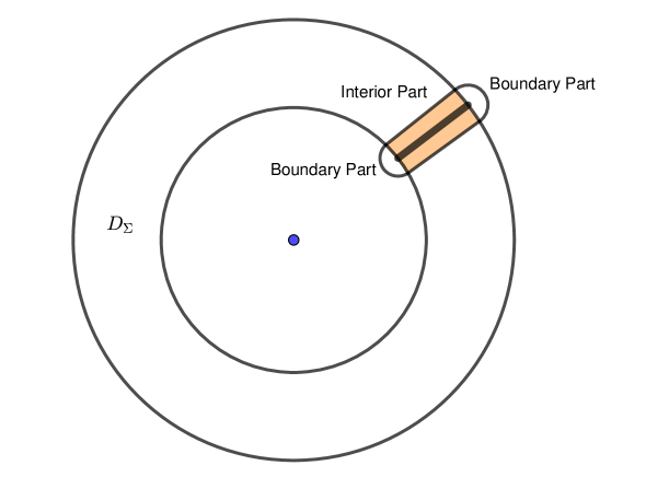
Figure 1. The neighborhood of $\Sigma_{\theta}$

As in Figure 1, the neighborhood $\mathcal{T}_{r}(\Sigma_{\theta})$ can be split into two parts.

Interior Part: $\mathcal{T}_{r}(\Sigma_{\theta})\cap D_{\Sigma}$. As in (2.9), using the above foliation, we have

(2.10) $$\|{\rm 1\rule{0.43057pt}{6.54443pt}\hskip 0.86108pt}_{\lambda}(P_{V})f\|_{L^{2}(\mathcal{T}_{r}(\Sigma_{\theta})\cap D_{\Sigma})}$$

$$\lesssim(\int_{|\phi-\theta|\leq r}\|{\rm 1\rule{0.43057pt}{6.54443pt}\hskip 0.86108pt}_{\lambda}(P_{V})f\|^{2}_{L^{2}(\Sigma_{\phi})}d\phi)^{\frac{1}{2}}$$

$$\lesssim r^{\frac{n-1}{2}}B\|f\|_{L^{2}(M)}.$$

Boundary Part: $\mathcal{T}_{r}(\Sigma_{\theta})\setminus D_{\Sigma}$. This part is essentially the $r$-neighborhood of $\partial\Sigma_{\theta}$, namely the endpoints of the curve $\Sigma_{\theta}$. Then by the $L^{\infty}$ bound in (1.7) we have

(2.11) $$\|{\rm 1\rule{0.43057pt}{6.54443pt}\hskip 0.86108pt}_{\lambda}(P_{V})f\|_{L^{2}(\mathcal{T}_{r}(\Sigma_{\theta})\setminus D_{\Sigma})}$$

$$\lesssim r^{\frac{n}{2}}\|{\rm 1\rule{0.43057pt}{6.54443pt}\hskip 0.86108pt}_{\lambda}(P_{V})f\|_{L^{\infty}(M)}$$

$$\lesssim r^{\frac{n}{2}}\lambda^{\frac{n-1}{2}}\|f\|_{L^{2}(M)}.$$

When $k=1$, $A=\lambda^{\frac{n-2}{2}}$ and $r=2^{\ell}\lambda^{-1}$, combining (2.10) with (2.11) we have for any $\theta\in S^{n-1}$

$$\lambda^{\frac{n-1}{2}}\|{\rm 1\rule{0.43057pt}{6.54443pt}\hskip 0.86108pt}_{\lambda}(P_{V})f\|_{L^{2}(\mathcal{T}_{r}(\Sigma_{\theta}))} \lesssim\lambda^{\frac{n-1}{2}}\cdot r^{\frac{n-1}{2}}B_{\Sigma}\|f\|_{L^{2}(M)}+\lambda^{\frac{n-1}{2}}\cdot\lambda^{\frac{n-1}{2}}r^{\frac{n}{2}}\|f\|_{L^{2}(M)}$$

$$=2^{\frac{n-1}{2}\ell}B\|f\|_{L^{2}(M)}+2^{\frac{n}{2}\ell}A\|f\|_{L^{2}(M)}.$$

Then we can estimate (2.7) for $\Sigma_{\theta}$ by

(2.12) $$\|K_{\ell}(V\cdot{\rm 1\rule{0.43057pt}{6.54443pt}\hskip 0.86108pt}_{\lambda}(P_{V})f)\|_{L^{2}(\Sigma_{\theta})}\lesssim(\varepsilon B+C_{\varepsilon}A)2^{-N\ell}\|f\|_{L^{2}(M)}.$$

Summing over $\ell$, we get the contribution $\varepsilon B+C_{\varepsilon}A$ in this case. Combing this with the contributions $O(A)$ from Cases 1-4, we get $B\leq\varepsilon B+C_{\varepsilon}A$, which implies $B\lesssim A$ as desired.

Remark 2.1.

Note that in the argument for $k=1$ we only use the fact that $S^{n-1}$ is a closed manifold. So the same argument works for any smooth embedding $\Phi:\Sigma\times Q\rightarrow D^{n}(10)$, where $Q$ is smooth closed manifold of dimension $n-1$ and $\Phi(\Sigma,\theta_{0})=\Sigma$ for some $\theta_{0}\in Q$. This fact will be used to deal with $k\geq 2$.

For $k\geq 2$, by rotation in local coordinates, one can similarly construct an embedding $\Phi:\Sigma\times S^{n-k}\rightarrow D^{n}(10)$. The Interior Part is similar, but the Boundary Part is more difficult to handle directly. To get around this difficulty, we generalize the family of embedded submanifolds and use an induction argument. Without loss of generality, we always assume $\Sigma$ is sufficiently small and homeomorhpic to a disk in $\mathbb{R}^{k}$.

Let

$$\mathcal{F}(\Sigma)=\{ (Q,\Phi):Q\text{ is a smooth closed manifold and }\dim Q=\dim M-\dim\Sigma,$$

$$\Phi:\Sigma\times Q\rightarrow D^{n}(10(n-k))\text{ is a smooth embedding},$$

$$\Phi(\Sigma,\theta_{0})=\Sigma\text{ for some }\theta_{0}\in Q\}.$$

From the above discussion, we see that $\mathcal{F}(\Sigma)$ is not empty.

Let $\Sigma_{\theta}=\Phi(\Sigma,\theta)$. We claim that for $n\geq 5$, $k\leq n-4$, $\dim\Sigma=k$, $(Q,\Phi)\in\mathcal{F}(\Sigma)$, there exists a constant $C=C(Q,\Phi,V,\Sigma,M)$ such that

(2.13) $$\sup_{\theta\in Q}\|{\rm 1\rule{0.43057pt}{6.54443pt}\hskip 0.86108pt}_{\lambda}(P_{V})\|_{L^{2}(M)\to L^{2}(\Sigma_{\theta})}\leq CA(k).$$

In the following, we establish (2.13) by an induction argument on $k$. The base case $k=1$ has been done as above. Suppose that (2.13) holds for submanifolds of dimension $k-1$. Now we prove it for submanifolds of dimension $k$.

Induction Step. We fix any $(Q,\Phi)\in\mathcal{F}(\Sigma)$, and let $D_{\Sigma}=\Phi(\Sigma,Q)$. As before, we will not distinguish $\Sigma_{x}$ and $D_{\Sigma}$ between their pullbacks, since the metrics are comparable the ones on $Q\times\Sigma$. Let

$$B=\sup_{\theta\in Q}\|{\rm 1\rule{0.43057pt}{6.54443pt}\hskip 0.86108pt}_{\lambda}(P_{V})\|_{L^{2}(M)\to L^{2}(\Sigma_{\theta})}.$$

By the $L^{\infty}$ bound in (1.7), we have $B\lesssim\lambda^{\frac{n-1}{2}}<+\infty.$ As before, the neighborhood $\mathcal{T}_{r}(\Sigma_{\theta})$ can be split into two parts.

Interior Part: $\mathcal{T}_{r}(\Sigma_{\theta})\cap D_{\Sigma}$, this contribution of this part can be handled as in (2.10) by $r^{\frac{n-k}{2}}B\|f\|_{L^{2}(M)}$.

Boundary Part: $\mathcal{T}_{r}(\Sigma_{\theta})\setminus D_{\Sigma}$ is essentially contained in $\mathcal{T}_{r}(\partial\Sigma_{\theta})$. We need to do some extensions in order to apply the induction hypothesis to $\partial\Sigma_{\theta}$, which is a smooth submanifold of dimension $k-1$.

Lemma 2.2 (Local extension lemma).

Let $Z\subset\mathbb{R}^{n}$ be a submanifold of dimension $k-1$. Suppose that we have an smooth embedding $\Phi:Z\times D^{n-k}(1)\rightarrow D^{n}(10(n-k))$ and $\Phi(Z,0)=Z$. Then for any $x_{0}\in Z$, there exist a neighborhood $U_{0}$ of $x_{0}$ in $Z$, and $\delta>0$, a smooth closed manifold $\tilde{Q}$ of dimension $n-k+1$, and an embedding $\phi:D^{n-k}(\delta)\to\tilde{Q}$, an embedding $\tilde{\Phi}:U_{0}\times\tilde{Q}\to D^{n}(10(n-k+1))$ that extends the region $\Phi(U_{0},D^{n-k}(\delta))$ in the following sense

$$\tilde{\Phi}(x,\phi(y))=\Phi(x,y)\ \ \text{ for }\ x\in U_{0},\ y\in D^{n-k}(\delta).$$

We postpone the proof of this lemma and use it to finish the induction argument. We first split $\partial\Sigma_{\theta}$ into finitely many small enough pieces. For each piece $Z$, by Lemma 2.2 we can find a neighborhood $U_{1}$ of $\theta$, such that we can extend $\Phi(Z,U_{1})$ to $\tilde{\Phi}(Z,\tilde{Q})$ for some $(\tilde{Q},\tilde{\Phi})\in\mathcal{F}(Z)$. Then by induction hypothesis, we have

$$\|{\rm 1\rule{0.43057pt}{6.54443pt}\hskip 0.86108pt}_{\lambda}(P_{V})f\|_{L^{2}(\mathcal{T}_{r}(\partial\Sigma_{\theta}))} \lesssim A(k-1)\cdot r^{\frac{n-(k-1)}{2}}\|f\|_{L^{2}(M)}$$

$$=A(k)\cdot\lambda^{-\frac{n-k}{2}}\cdot 2^{\frac{n-k+1}{2}\ell}\|f\|_{L^{2}(M)}.$$

By the compactness of $Q$, we can choose a constant uniform in $\theta\in Q$. Thus for $r=2^{\ell}\lambda^{-1}$, we have

$$\lambda^{\frac{n-k}{2}}\|{\rm 1\rule{0.43057pt}{6.54443pt}\hskip 0.86108pt}_{\lambda}(P_{V})f\|_{L^{2}(\mathcal{T}_{r}(\Sigma_{\theta}))}\lesssim 2^{\frac{n-k}{2}\ell}B\|f\|_{L^{2}(M)}+A(k)\cdot 2^{\frac{n-k+1}{2}\ell}\|f\|_{L^{2}(M)}.$$

Note that $N$ can be arbitrarily large in (2.7). Summing over $\ell$, we get the contribution $\varepsilon B+C_{\varepsilon}A$ in this case. Finally, combing this with the contributions $O(A)$ from Cases 1-4, we have $B\leq\varepsilon B+C_{\varepsilon}A$, which implies $B\lesssim A$ as desired.

Proof of Lemma 2.2.

Let $x=(x_{1},\cdots,x_{k-1})$ be a local coordinate near $x_{0}$ on $Z$ and assume $x_{0}=0$. Let $\Phi_{1}(x,w)=s\nu+\Phi(x,y)$, where $w=(y,s)$ and $\nu\in{\mathbb{R}}^{n}$ is a unit normal vector of $\Phi(Z,D^{n-k}(1))$ at $\Phi(x_{0},0)$. Then we can find $\delta_{1}>0$ and a neighborhood $U_{0}$ of $x_{0}$ such that

$$\Phi_{1}:U_{0}\times D^{n-k+1}(\delta_{1})\to D^{n}(10(n-k))$$

is a smooth embedding.

Let $e_{i}=\partial_{x_{i}}\Phi_{1}(0,0)$ for $1\leq i\leq k-1$, and $f_{j}=\partial_{w_{j}}\Phi_{1}(0,0)$ for $1\leq j\leq n-k+1$. By a linear transformation, we may assume $\{e_{i}\}\cup\{f_{j}\}$ is an orthonormal basis of ${\mathbb{R}}^{n}$. We extend $\Phi_{1}(0,D^{n-k+1}(\delta_{1}))$ to a smooth closed manifold $\tilde{Q}\subset D^{n-k+1}(10\delta_{1})$ that is homeomorhpic to the sphere $S^{n-k+1}$. Fix a sufficiently small $\delta_{2}>0$ and let $\mathcal{T}_{\delta_{2}}(\tilde{Q})\subset{\mathbb{R}}^{n}$ be the $\delta_{2}$-neighborhood of $\tilde{Q}$. Then using the normal vector fields of $\tilde{Q}$, one can find a smooth bijection

$$\Phi_{2}:D^{k-1}(\delta_{2})\times\tilde{Q}\to\mathcal{T}_{\delta_{2}}(\tilde{Q})$$

such that for each $q\in\tilde{Q}$, $\Phi_{2}(\cdot,q)$ is an isometry, and $\Phi_{2}(D^{k-1}(\delta_{2}),q)$ is a disk centered at $q$ and lies in the normal plane of $\tilde{Q}$ at $q$. We can choose the above $w\in D^{n-k+1}(\delta_{1})$ as a local coordinate over $\Phi_{1}(0,D^{n-k+1}(\delta_{1}))\subset\tilde{Q}$. We will not distinguish the local coordinate and the corresponding point in the later calculations.

Let $\bar{e}_{i}=\partial_{x_{i}}\Phi_{2}(0,0)$ for $1\leq i\leq k-1$, and $\bar{f}_{j}=\partial_{w_{j}}\Phi_{2}(0,0)$ for $1\leq j\leq n-k+1$. We have $\bar{f}_{j}=f_{j}$ since $\Phi_{1}(0,w)=\Phi_{2}(0,w)$ for $w$ near 0. Since both $\{e_{i}\}$ and $\{\bar{e}_{i}\}$ form an orthonormal basis of the normal plane of $\tilde{Q}$ at $w=0$, by applying a suitable orthogonal transformation, we may assume $\bar{e}_{i}=e_{i}$. By continuity, for any $\varepsilon>0$, we can choose $\delta$ small enough such that when $|x|<\delta,\ |w|<\delta$, we have

(2.14) $$|\partial_{x_{i}}\Phi_{\alpha}(x,w)-e_{i}|<\varepsilon\ \ \text{and}\ \ |\partial_{w_{j}}\Phi_{\alpha}(x,w)-f_{j}|<\varepsilon$$

for $\alpha=1,2$ and $1\leq i\leq k-1$ and $1\leq j\leq n-k+1.$ Choose a cutoff function $\eta\in C_{0}^{\infty}(D^{n-k+1}(\delta))$ with $\eta(w)=1$ in $D^{n-k+1}(\delta/2)$, and let

$$\tilde{\Phi}(x,w)=\eta(w)\Phi_{1}(x,w)+(1-\eta(w))\Phi_{2}(x,w).$$

Then for $|x|<\delta,\ |w|<\delta$, $\tilde{\Phi}(x,w)$ satisfies the same derivative estimates as in (2.14), and so its Jacobian has full rank when $\varepsilon$ is sufficiently small. So

$$\tilde{\Phi}:D^{k-1}(\delta)\times\tilde{Q}\to D^{n}(10(n-k+1))$$

is the desired embedding. ∎

3. Remove the log loss in Case 2

In this section, we refine the argument in Case 2 and remove the log loss. Note that the resolvent-like symbol $(\lambda_{j}^{2}-\tau_{k}^{2})^{-1}$ naturally appears in the previous perturbation argument for the wave kernels. To remove the log loss, we shall use the kernel decomposition of the resolvent operator $(-\Delta_{g}-\lambda^{2}+i\lambda)^{-1}$ in [14] and [46].

Case 2. $|\tau_{k}-\lambda|\leq 1$, $|\lambda_{j}-\lambda|\in(2^{\ell},2^{\ell+1}]$, $1\leq 2^{\ell}\leq\lambda$.

Recall that we split the frequencies by the cutoff function $\psi\in C_{0}^{\infty}(\mathbb{R})$ satisfying $\psi(t)=1$ if $|t|\leq 2$ and $\psi(t)=0$ if $|t|>3$. In this case, $m(\lambda_{j},\tau_{k})=\frac{-\chi_{\lambda}(\tau_{k})}{\lambda_{j}^{2}-\tau_{k}^{2}}\psi(\lambda_{j}/\lambda)$. Let

$$m_{1}(\lambda_{j},\tau_{k})=\frac{-\chi_{\lambda}(\tau_{k})}{\lambda_{j}^{2}-\tau_{k}^{2}+i\lambda}\psi(\lambda_{j}/\lambda)$$

and

$$m_{2}(\lambda_{j},\tau_{k})=m(\lambda_{j},\tau_{k})-m_{1}(\lambda_{j},\tau_{k}).$$

We first handle $m_{2}$. It is clear that

(3.1) $$m_{2}(\lambda_{j},\tau_{k})=\frac{-i\lambda\chi_{\lambda}(\tau_{k})}{(\lambda_{j}^{2}-\tau_{k}^{2})(\lambda_{j}^{2}-\tau_{k}^{2}+i\lambda)}\psi(\lambda_{j}/\lambda).$$

For $|s-\lambda|\leq 1$ and $|\lambda_{j}-\lambda|\in(2^{\ell},2^{\ell+1}]$, we have

$$|m_{2}(\lambda_{j},s)|+|\partial_{s}m_{2}(\lambda_{j},s)|\lesssim\lambda^{-1}2^{-2\ell}.$$

We can use the same argument as Case 1 to handle

$$\sum_{|\lambda_{j}-\lambda|\in(2^{\ell},2^{\ell+1}]}\sum_{|\tau_{k}-\lambda|\leq 1}\int_{M}m_{2}(\lambda_{j},\tau_{k})e_{j}^{0}(x)e_{j}^{0}(z)e_{\tau_{k}}(z)e_{\tau_{k}}(y)V(z)dz$$

$$=\sum_{|\lambda_{j}-\lambda|\in(2^{\ell},2^{\ell+1}]}\sum_{|\tau_{k}-\lambda|\leq 1}\int_{M}\int_{\lambda-1}^{\lambda+1}\partial_{s}m_{2}(\lambda_{j},s){\rm 1\rule{0.43057pt}{6.54443pt}\hskip 0.86108pt}_{[\lambda-1,\tau_{k}]}(s)e_{j}^{0}(x)e_{j}^{0}(z)e_{\tau_{k}}(z)e_{\tau_{k}}(y)V(z)dzds$$

$$\ \ \ +\sum_{|\lambda_{j}-\lambda|\in(2^{\ell},2^{\ell+1}]}\sum_{|\tau_{k}-\lambda|\leq 1}\int_{M}m_{2}(\lambda_{j},\lambda-1)e_{j}^{0}(x)e_{j}^{0}(z)e_{\tau_{k}}(z)e_{\tau_{k}}(y)V(z)dz$$

$$=K_{1,\ell}(x,y)+K_{2,\ell}(x,y).$$

We handle $K_{2,\ell}$ first. For any $f\in L^{2}(M)$, we have

$$\|K_{2,\ell}f\|_{L^{p_{c}}(\Sigma)} =\|{\rm 1\rule{0.43057pt}{6.54443pt}\hskip 0.86108pt}_{\lambda,\ell}(P^{0})m(P^{0},\lambda-1)(V\cdot{\rm 1\rule{0.43057pt}{6.54443pt}\hskip 0.86108pt}_{\lambda}(P_{V})f)\|_{L^{p_{c}}(\Sigma)}$$

$$\lesssim A2^{\ell/2}\|{\rm 1\rule{0.43057pt}{6.54443pt}\hskip 0.86108pt}_{\lambda,\ell}(P^{0})m(P^{0},\lambda-1)(V\cdot{\rm 1\rule{0.43057pt}{6.54443pt}\hskip 0.86108pt}_{\lambda}(P_{V})f)\|_{L^{2}}$$

$$\lesssim A\lambda^{-1}2^{-3\ell/2}\|{\rm 1\rule{0.43057pt}{6.54443pt}\hskip 0.86108pt}_{\lambda,\ell}(P^{0})(V\cdot{\rm 1\rule{0.43057pt}{6.54443pt}\hskip 0.86108pt}_{\lambda}(P_{V})f)\|_{L^{2}}$$

$$\lesssim A\lambda^{-1+\sigma(p_{0})}2^{-\ell}\|V\cdot{\rm 1\rule{0.43057pt}{6.54443pt}\hskip 0.86108pt}_{\lambda}(P_{V})f\|_{L^{p_{0}^{\prime}}}$$

$$\lesssim A\lambda^{-1+\sigma(p_{0})}2^{-\ell}\|V\|_{L^{q}}\|{\rm 1\rule{0.43057pt}{6.54443pt}\hskip 0.86108pt}_{\lambda}(P_{V})f\|_{L^{q_{0}}}$$

$$\lesssim A\lambda^{-1+\sigma(p_{0})+\sigma(q_{0})}2^{-\ell}\|V\|_{L^{q}}\|f\|_{L^{2}}$$

$$=A2^{-\ell}\|V\|_{L^{q}}\|f\|_{L^{2}}$$

The method to handle $K_{1,\ell}$ is similar. Note that there is no log loss if we sum over $\ell$.

Next, we handle $m_{1}$. It suffices to deal with $m_{1}(\lambda_{j},\tau_{k})$ for all $\lambda_{j}\leq 3\lambda$, as the easy case $|\lambda_{j}-\lambda|\leq 1$ can be handled similarly as in Case 1.

We write

$$\sum_{\lambda_{j}}\sum_{|\tau_{k}-\lambda|\leq 1}\int_{M}m_{1}(\lambda_{j},\tau_{k})e_{j}^{0}(x)e_{j}^{0}(z)e_{\tau_{k}}(z)e_{\tau_{k}}(y)V(z)dz$$

$$=\sum_{\lambda_{j}}\sum_{|\tau_{k}-\lambda|\leq 1}\int_{M}\int_{\lambda-1}^{\lambda+1}\partial_{s}m_{1}(\lambda_{j},s){\rm 1\rule{0.43057pt}{6.54443pt}\hskip 0.86108pt}_{[\lambda-1,\tau_{k}]}(s)e_{j}^{0}(x)e_{j}^{0}(z)e_{\tau_{k}}(z)e_{\tau_{k}}(y)V(z)dzds$$

$$\ \ \ +\sum_{\lambda_{j}}\sum_{|\tau_{k}-\lambda|\leq 1}\int_{M}m_{1}(\lambda_{j},\lambda-1)e_{j}^{0}(x)e_{j}^{0}(z)e_{\tau_{k}}(z)e_{\tau_{k}}(y)V(z)dz$$

$$=K_{1}(x,y)+K_{2}(x,y).$$

For $|s-\lambda|\leq 1$, we have

$$|m_{1}(\lambda_{j},s)|+|\partial_{s}m_{1}(\lambda_{j},s)|\lesssim\lambda^{-1}.$$

As before, we just handle $K_{2}$. It suffices to prove for each $s\in[\lambda-1,\lambda+1]$

(3.2) $$\|(-\Delta_{g}-s^{2}+i\lambda)^{-1}\psi(P^{0}/\lambda)\|_{L^{p_{0}^{\prime}}(M)\to L^{p_{c}}(\Sigma)}\lesssim A\lambda^{\sigma(p_{0})-1}.$$

Indeed, by (3.2) we have

$$\|m_{1}(P^{0},\lambda-1)(V\cdot{\rm 1\rule{0.43057pt}{6.54443pt}\hskip 0.86108pt}_{\lambda}(P_{V})f)\|_{L^{p_{c}}(\Sigma)} \lesssim A\lambda^{\sigma(p_{0})-1}\|V\cdot{\rm 1\rule{0.43057pt}{6.54443pt}\hskip 0.86108pt}_{\lambda}(P_{V})f\|_{L^{p_{0}^{\prime}}}$$

$$\lesssim A\lambda^{\sigma(p_{0})-1}\|V\|_{L^{q}}\|{\rm 1\rule{0.43057pt}{6.54443pt}\hskip 0.86108pt}_{\lambda}(P_{V})f\|_{L^{q_{0}}}$$

$$\lesssim A\lambda^{\sigma(p_{0})-1+\sigma(q_{0})}\|V\|_{L^{q}}\|f\|_{L^{2}}$$

$$=A\|V\|_{L^{q}}\|f\|_{L^{2}}.$$

We first handle $n=2$ for $V\in\mathcal{K}(M)$ by Hadamard parametrix. Recall that $p_{c}=4$ and $p_{0}=q_{0}=\infty$ in this case. For each $s\in[\lambda-1,\lambda+1]$, we write as in [4, Proof of Theorem 5.1]

(3.3) $$(-\Delta_{g}-s^{2}+i\lambda)^{-1}\psi(P^{0}/\lambda)=T_{\lambda}+R_{\lambda},$$

where $R_{\lambda}$ is a non-local operator which satisfies

$$\|R_{\lambda}\|_{L^{1}(M)\to L^{p_{c}}(\Sigma)}\lesssim\lambda^{\delta(p_{c})+\sigma(\infty)-1}=A\lambda^{\sigma(p_{0})-1}.$$

And $T_{\lambda}$ is a local operator, which satisfies following kernel estimates

(3.4) $$|T_{\lambda}(x,y)|\lesssim\begin{cases}|\log(\lambda d_{g}(x,y)/2)|,\hskip 5.69054pt\ \ \ \text{if}\hskip 5.69054ptd_{g}(x,y)\leq\lambda^{-1}\\ \lambda^{-1/2}\big{(}d_{g}(x,y)\big{)}^{-1/2},\hskip 5.69054pt\text{if}\hskip 5.69054pt\lambda^{-1}\leq d_{g}(x,y)\leq 1.\\ \end{cases}$$

By Young’s inequality, we have

$$\|T_{\lambda}\|_{L^{1}(M)\to L^{p_{c}}(\Sigma)}\lesssim\lambda^{-\frac{1}{4}}=A\lambda^{\sigma(p_{0})-1}.$$

Similarly, for the special endpoint $p=2$ we have

$$\|R_{\lambda}\|_{L^{1}(M)\to L^{2}(\Sigma)}\lesssim\lambda^{\delta(2)+\sigma(\infty)-1}=A\lambda^{\sigma(p_{0})-1}$$

$$\|T_{\lambda}\|_{L^{1}(M)\to L^{2}(\Sigma)}\lesssim\lambda^{-\frac{1}{2}}(\log\lambda)^{\frac{1}{2}}\lesssim A\lambda^{\sigma(p_{0})-1}.$$

Moreover, these still hold if $\Sigma$ has non-vanishing curvature.

Next, we consider $n\geq 3$. As in [14] and [46], we write

(3.5) $$(-\Delta_{g}-s^{2}+i\lambda)^{-1}\psi(P^{0}/\lambda)=(S_{0}(P^{0})+\sum_{j\geq 1}S_{j}(P^{0})+R_{\lambda}(P^{0}))\psi(P^{0}/\lambda).$$

Here

(3.6) $$|S_{0}(\tau)\psi(\tau/\lambda)|\lesssim\lambda^{-2}{\rm 1\rule{0.43057pt}{6.54443pt}\hskip 0.86108pt}_{\leq 3\lambda}(\tau)$$

and for $1\leq j\lesssim\log\lambda$

(3.7) $$|S_{j}(\tau)\psi(\tau/\lambda)|\lesssim\lambda^{-1}\varepsilon(1+\varepsilon|\lambda-\tau|)^{-N},\ \ \forall N.$$

and

(3.8) $$|R_{\lambda}(\tau)\psi(\tau/\lambda)|\lesssim\lambda^{-1}((1+|\lambda-\tau|)^{-N}+(1+|\lambda+\tau|)^{-N}),\ \ \forall N.$$

By the spectral projection bounds (1.8), (1.7) and the symbol estimates (3.6), (3.7), (3.8), it is easy to use a duality argument to obtain (see e.g. [14, Proof of Lemma 2.3])

(3.9) $$\|S_{0}(P^{0})\psi(P^{0}/\lambda)\|_{L^{p_{0}^{\prime}}(M)\to L^{p_{c}}(\Sigma)}\lesssim A\lambda^{\sigma(p_{0})-1},$$

(3.10) $$\|S_{j}(P^{0})\psi(P^{0}/\lambda)\|_{L^{p_{0}^{\prime}}(M)\to L^{p_{c}}(\Sigma)}\lesssim A\lambda^{\sigma(p_{0})-1},$$

(3.11) $$\|R_{\lambda}(P^{0})\psi(P^{0}/\lambda)\|_{L^{p_{0}^{\prime}}(M)\to L^{p_{c}}(\Sigma)}\lesssim A\lambda^{\sigma(p_{0})-1}.$$

However, we will get a log loss after summing over $1\leq j\lesssim\log\lambda$. To get around this, we need to improve (3.10). By the proof of the kernel estimate of $S_{j}(P^{0})$ in [46, (2.23)], we can obtain the kernel of its smooth cutoff in essentially the same form

(3.12) $$S_{j}(P_{0})\psi(P_{0}/\lambda)(x,y)=\lambda^{\frac{n-3}{2}}\varepsilon^{-\frac{n-1}{2}}e^{i\lambda d_{g}(x,y)}a_{\varepsilon}(x,y)+O(\lambda^{-1}\varepsilon^{1-n}{\rm 1\rule{0.43057pt}{6.54443pt}\hskip 0.86108pt}_{d_{g}(x,y)<4\varepsilon})$$

where $\varepsilon=\lambda^{-1}2^{j}$ and the smooth function $a_{\varepsilon}(x,y)$ is supported in $\{d_{g}(x,y)/\varepsilon\in(1/4,4)\}$ and

$$|\partial_{x,y}^{\gamma}a_{\varepsilon}(x,y)|\leq C_{\gamma}\varepsilon^{-|\gamma|}.$$

We denote the first term by $T_{j}(x,y)$ and the remainder term by $r_{j}(x,y)$.

Let us handle the remainder term first. By Young’s inequality

$$\|r_{j}f\|_{L^{p_{c}}(\Sigma)} \lesssim\lambda^{-1}\varepsilon^{1-n}\cdot\varepsilon^{\frac{k}{p_{c}}+\frac{n}{p_{0}}}\|f\|_{L^{p_{0}^{\prime}}(M)}$$

$$=\lambda^{n-2-\frac{k}{p_{c}}-\frac{n}{p_{0}}}2^{j(1-n+\frac{k}{p_{c}}+\frac{n}{p_{0}})}\|f\|_{L^{p_{0}^{\prime}}(M)}$$

Since $p_{c}=2$ when $k\leq n-2$ and $p_{c}=\frac{2n}{n-1}$ when $k=n-1$, we have

$$n-2-\frac{k}{p_{c}}-\frac{n}{p_{0}}=\delta(p_{c})+\sigma(p_{0})-1,$$

$$1-n+\frac{k}{p_{c}}+\frac{n}{p_{0}}<0.$$

So summing over $j$ we get

$$\sum_{j}\|r_{j}f\|_{L^{p_{c}}(\Sigma)}\lesssim\lambda^{\delta(p_{c})+\sigma(p_{0})-1}\|f\|_{L^{p_{0}^{\prime}}(M)}.$$

The special endpoint $p=2$ for $k=n-1$ also follows from the same argument with $p_{c}$ replaced by 2.

It remains to handle $T_{j}$. Let $\{x_{\ell}\}$ be a maximal $\varepsilon$-separated set in $\Sigma$. Suppose that $\rho_{\varepsilon}$ is a smooth cutoff function on $\Sigma$ with support of diameter $\sim\varepsilon$, and $\eta_{\varepsilon}$ is a smooth cutoff function on $M$ with support of diameter $\sim\varepsilon$, and $\{\rho_{\varepsilon}(x-x_{\ell})\}$ is a partition of unity on $\Sigma$. Let $T^{\lambda}$ be the oscillatory integral operator

(3.13) $$T^{\lambda}f(x)=\int_{M}e^{i\lambda d_{g}(x,y)}a(x,y)f(y)dy,$$

where $dy$ is the volume measure on $M$, and the smooth function $a(x,y)$ is supported in $\{d_{g}(x,y)\in(\frac{1}{4},4)\}$ and $|\partial_{x,y}^{\gamma}a(x,y)|\leq C_{\gamma}.$ By the proof of the $L^{2}(M)-L^{p_{c}}(\Sigma)$ bound (1.8) and interpolation with the trivial $L^{1}(M)-L^{p_{c}}(\Sigma)$ bound, we have for some $\delta_{0}>0$

(3.14) $$\|T^{\lambda}\|_{L^{p_{0}^{\prime}}(M)\to L^{p_{c}}(\Sigma)}\lesssim\lambda^{-\frac{2k}{p_{0}p_{c}}}\lesssim\lambda^{\frac{n-1}{2}-\frac{n}{p_{0}}-\frac{k}{p_{c}}-\delta_{0}},$$

whenever

(3.15) $$k<\frac{p_{c}}{2}\Big{(}n-\frac{1}{1-2/p_{0}}\Big{)}.$$

Note that if $T^{\lambda}$ is just the spectral projection operator in [50, (5.1.3’)] modulo the factor $\lambda^{\frac{n-1}{2}}$ and a remainder term, then (3.14) beats the simple bound from the duality argument (see e.g. [14, Proof of Lemma 2.3]). Here we only focus on the power gain, so we omit the log loss that possibly appears in (3.14) when $k=n-2$.

So by rescaling and using (3.14) we have

$$\|T_{j}f\|_{L^{p_{c}}(\Sigma)}=\lambda^{\frac{n-3}{2}}\varepsilon^{-\frac{n-1}{2}}(\sum_{\ell}\int_{\Sigma}\Big{|}\int_{M}e^{i\lambda d_{g}(x,y)}a_{\varepsilon}(x,y)\rho_{\varepsilon}(x-x_{\ell})\eta_{\varepsilon}(y-x_{\ell})f(y)dy\Big{|}^{p_{c}}dx)^{\frac{1}{p_{c}}}$$

$$=\lambda^{\frac{n-3}{2}}\varepsilon^{-\frac{n-1}{2}}\varepsilon^{n+\frac{k}{p_{c}}}(\sum_{\ell}\int_{\Sigma}\Big{|}\int_{M}e^{i\lambda d_{g}(\varepsilon x+x_{\ell},\varepsilon y+x_{\ell})}a_{\varepsilon}(\varepsilon x+x_{\ell},\varepsilon y+x_{\ell})\rho_{\varepsilon}(\varepsilon x)\eta_{\varepsilon}(\varepsilon y)f(\varepsilon y+x_{\ell})dy\Big{|}^{p_{c}}dx)^{\frac{1}{p_{c}}}$$

$$\lesssim\lambda^{\frac{n-3}{2}}\varepsilon^{-\frac{n-1}{2}}\varepsilon^{n+\frac{k}{p_{c}}}2^{j(\frac{n-1}{2}-\frac{n}{p_{0}}-\frac{k}{p_{c}}-\delta_{0})}(\sum_{\ell}\|\eta_{\varepsilon}(\varepsilon y)f(\varepsilon y+x_{\ell})\|_{L^{p_{0}^{\prime}}(M)}^{p_{c}})^{\frac{1}{p_{c}}}$$

$$\lesssim\lambda^{\frac{n-3}{2}}\varepsilon^{-\frac{n-1}{2}}\varepsilon^{n+\frac{k}{p_{c}}}2^{j(\frac{n-1}{2}-\frac{n}{p_{0}}-\frac{k}{p_{c}}-\delta_{0})}(\sum_{\ell}\|\eta_{\varepsilon}(\varepsilon y)f(\varepsilon y+x_{\ell})\|_{L^{p_{0}^{\prime}}(M)}^{p_{0}^{\prime}})^{\frac{1}{p_{0}^{\prime}}}$$

$$\lesssim\lambda^{\frac{n-3}{2}}\varepsilon^{-\frac{n-1}{2}}\varepsilon^{n+\frac{k}{p_{c}}}2^{j(\frac{n-1}{2}-\frac{n}{p_{0}}-\frac{k}{p_{c}}-\delta_{0})}\varepsilon^{-n/p_{0}^{\prime}}\|f\|_{L^{p_{0}^{\prime}}(M)}$$

$$=\lambda^{n-2-\frac{k}{p_{c}}-\frac{n}{p_{0}}}2^{-\delta_{0}j}\|f\|_{L^{p_{0}^{\prime}}(M)}.$$

So summing over $j$ we get

$$\sum_{j}\|T_{j}f\|_{L^{p_{c}}(\Sigma)}\lesssim\lambda^{\delta(p_{c})+\sigma(p_{0})-1}\|f\|_{L^{p_{0}^{\prime}}(M)}.$$

Since $\frac{1}{p_{0}}\in[\frac{n+3}{2n+2}-\frac{2}{n},\frac{n-1}{2n+2}]$, by (3.15) we see that the range of admissible $k$ is

$$k<\frac{p_{c}}{2}\Big{(}n-\frac{1}{1-2(\frac{n+3}{2n+2}-\frac{2}{n})}\Big{)}=\frac{p_{c}}{2}\cdot\frac{n(n+3)}{2(n+2)}.$$

When $k\leq n-2$ and $p_{c}=2$, this is equivalent to $k<\frac{n+1}{2}-\frac{1}{n+2}$. So $k\leq n/2$. When $k=n-1$ and $p_{c}=\frac{2n}{n-1}$, this is equivalent to $n^{3}-3n^{2}-6n+4<0$. So $n=3,4.$ The special endpoint $p=2$ when $k=n-1$ also holds for $n=3,4$ and we shall discuss it in the following subsection.

Remark 3.1.

Let $n\geq 3$. To remove the log loss in Case 2, it suffices to establish

(3.16) $$\|T^{\lambda}\|_{L^{p_{0}^{\prime}}(M)\to L^{p_{c}}(\Sigma)}\lesssim\lambda^{\frac{n-1}{2}-\frac{n}{p_{0}}-\frac{k}{p_{c}}-\delta_{0}}$$

for some $\delta_{0}>0$ and $\frac{1}{p_{0}}\in[\frac{n+3}{2n+2}-\frac{2}{n},\frac{n-1}{2n+2}]$. It is proved for $k\leq n/2$ when $n\geq 5$ and for all $k$ when $n\leq 4$. Moreover, in Section 5 we shall discuss it further in the model case where the metric is Euclidean and the submanifold is flat. In this case, we can improve the range to $k\leq[2n/3]-2$ when $n\geq 11$.

3.1. Remove the log loss for certain exponents

Since we have only discussed the endpoint $L^{p_{c}}(\Sigma)$ norm so far, we shall refine the interpolation argument above and also remove the log loss for certain exponents $p$, such as the special endpoint $p=2$ when $k=n-1$.

Let $n\geq 3$. We first handle $p\geq p_{c}$. Suppose that for some $\alpha\geq 0$

(3.17) $$\|T^{\lambda}\|_{L^{p_{0}^{\prime}}(M)\to L^{p}(\Sigma)}\lesssim\lambda^{-\alpha}.$$

Then by the previous argument we get

(3.18) $$\|T_{j}\|_{L^{p_{0}^{\prime}}(M)\to L^{p}(\Sigma)}\lesssim\lambda^{n-2-\frac{k}{p}-\frac{n}{p_{0}}}2^{j(-\alpha-\frac{n-1}{2}+\frac{n}{p_{0}}+\frac{k}{p})}.$$

To remove the log loss, we require that

(3.19) $$n-2-\frac{k}{p}-\frac{n}{p_{0}}+\sigma(q_{0})\leq\frac{n-1}{2}-\frac{k}{p}$$

(3.20) $$n-2-\frac{k}{p}-\frac{n}{p_{0}}+(-\alpha-\frac{n-1}{2}+\frac{n}{p_{0}}+\frac{k}{p})+\sigma(q_{0})<\frac{n-1}{2}-\frac{k}{p}.$$

To get the largest range of $p$, we require that $q_{0}=\frac{2n+2}{n-1}$ and $\frac{1}{p_{0}}=\frac{n+3}{2n+2}-\frac{2}{n}$. Then (3.19) always holds, and (3.20) is equivalent to

(3.21) $$\alpha>\frac{k}{p}-\frac{n+3}{2n+2}.$$

Now it suffices to determine the best $\alpha$ in (3.17).

When $k=n-1$, by interpolation between $L^{2}-L^{2}$ and $L^{1}-L^{\infty}$ bounds we have

(3.22) $$\|T^{\lambda}\|_{L^{p^{\prime}}(M)\to L^{p}(\Sigma)}\lesssim\lambda^{-\frac{1}{p}(n-\frac{3}{2})}.$$

By Stein’s oscillatory integral theorem (see [50, Theorem 2.2.1]), we get

(3.23) $$\|T^{\lambda}\|_{L^{\frac{2n}{n+2}}(M)\to L^{2}(\Sigma)}\lesssim\lambda^{-\frac{(n-1)(n-2)}{2n}}.$$

By the interpolation between this and the $L^{1}-L^{\infty}$ bound, we get for $p_{2}=\frac{np}{n-2}$

(3.24) $$\|T^{\lambda}\|_{L^{p_{2}^{\prime}}(M)\to L^{p}(\Sigma)}\lesssim\lambda^{-(n-1)/p_{2}}.$$

We require that $p<p_{0}<p_{2}$. By interpolation between (3.22) and (3.24) we get

(3.25) $$\|T^{\lambda}\|_{L^{p_{0}^{\prime}}(M)\to L^{p}(\Sigma)}\lesssim\lambda^{-\frac{n-2}{4p}-\frac{3n-4}{4p_{0}}}.$$

When $k\geq n-2$, similarly we have

(3.26) $$\|T^{\lambda}\|_{L^{p^{\prime}}(M)\to L^{p}(\Sigma)}\lesssim\lambda^{-k/p},$$

and for $p_{2}=\frac{(k+1)p}{k-1}$

(3.27) $$\|T^{\lambda}\|_{L^{p_{2}^{\prime}}(M)\to L^{p}(\Sigma)}\lesssim\lambda^{-k/p_{2}}.$$

We require that $p<p_{0}<p_{2}$. By interpolation between (3.26) and (3.27) we get

(3.28) $$\|T^{\lambda}\|_{L^{p_{0}^{\prime}}(M)\to L^{p}(\Sigma)}\lesssim\lambda^{-k/p_{0}}.$$

Thus, inserting the power $\alpha$ from (3.25) and (3.28) into (3.21), we can obtain the range of $p$. When $k=n-1$, we have

$$p>\frac{2n(-2+n+3n^{2})}{16+4n-3n^{2}+3n^{3}}=2+\frac{8}{3n}-\frac{4}{3n^{2}}+O(\frac{1}{n^{3}})$$

for $n\geq 9$, and $p\geq p_{c}$ for $n\leq 8$. When $k\leq n-2$, we have

$$p>\frac{2kn(n+1)}{k(n^{2}-n-4)+n^{2}+3n}=2+\frac{2(k+1)}{n^{2}}+O(\frac{1}{n^{3}}).$$

Moreover, we can also consider $2\leq p<p_{c}$ when $n\leq 8$ and $k=n-1$. To remove the log loss, we require that

(3.29) $$n-2-\frac{n-1}{p}-\frac{n}{p_{0}}+\sigma(q_{0})\leq\frac{n-1}{4}-\frac{n-2}{2p}$$

(3.30) $$n-2-\frac{n-1}{p}-\frac{n}{p_{0}}+(-\alpha-\frac{n-1}{2}+\frac{n}{p_{0}}+\frac{n-1}{p})+\sigma(q_{0})<\frac{n-1}{4}-\frac{n-2}{2p}.$$

To get the largest range of $p$, we require that $q_{0}=\frac{2n+2}{n-1}$ and $\frac{1}{p_{0}}=\frac{n+3}{2n+2}-\frac{2}{n}$. Then (3.29) always holds, and (3.30) is equivalent to

(3.31) $$\alpha>\frac{n-2}{2p}+\frac{n^{2}-2n-7}{4(n+1)}.$$

Now it suffices to determine the best $\alpha$ in (3.17). Indeed, we can interpolate between (3.24) and the trivial bound

(3.32) $$\|T^{\lambda}\|_{L^{1}(M)\to L^{p}(\Sigma)}\lesssim 1$$

to get

(3.33) $$\|T^{\lambda}\|_{L^{p_{0}^{\prime}}(M)\to L^{p}(\Sigma)}\lesssim\lambda^{-(n-1)/p_{0}}.$$

Thus, inserting the power $\alpha$ from (3.33) (when $n\leq 6$) or (3.25) (when $n\geq 7$) into (3.31) we get

$$p>\begin{cases}6/5=1.200,\ \ \ \ \ \ \ \ n=3\\ 20/11\approx 1.818,\ \ \ \ \ n=4\\ 45/22\approx 2.045,\ \ \ \ \ n=5\\ 168/79\approx 2.127,\ \ \ \ n=6\\ 280/127\approx 2.205,\ \ \ n=7\\ 9/4=2.250,\ \ \ \ \ \ \ \ \ n=8.\end{cases}$$

But $p\geq 2$. So in particular we can handle the special endpoint $p=2$ when $n=3,4$.

Special case: Curved hypersurfaces. Recall that when $k=n-1$ there is a power improvement for $2\leq p<p_{c}$ if $\Sigma$ has non-vanishing Gaussian curvature. We have handled $n=2$ in the previous discussion. Now we handle $n\geq 3$. We first consider $p\geq p_{c}$. For the curved case, by interpolation between the curved $L^{2}-L^{2}$ bound and the trivial $L^{1}-L^{\infty}$ bounds we have

(3.34) $$\|T^{\lambda}\|_{L^{p^{\prime}}(M)\to L^{p}(\Sigma)}\lesssim\lambda^{-\frac{1}{p}(n-\frac{4}{3})}.$$

By interpolation between (3.34) and (3.24) we get

(3.35) $$\|T^{\lambda}\|_{L^{p_{0}^{\prime}}(M)\to L^{p}(\Sigma)}\lesssim\lambda^{-\frac{n-2}{6p}-\frac{5n-6}{6p_{0}}}.$$

Thus, inserting the power $\alpha$ from (3.35) into (3.21), we can obtain

$$p>\frac{2(-4n+n^{2}+5n^{3})}{24+4n-5n^{2}+5n^{3}}=2+\frac{12}{5n}-\frac{4}{5n^{2}}+O(\frac{1}{n^{3}})$$

for $n\geq 11$, and $p\geq p_{c}$ for $n\leq 10$. These ranges are larger than the general case.

Next, we can still consider $2\leq p<p_{c}$ for $n\leq 10$. To remove the log loss, we require

(3.36) $$n-2-\frac{n-1}{p}-\frac{n}{p_{0}}+\sigma(q_{0})\leq\frac{n-1}{3}-\frac{2n-3}{3p}$$

(3.37) $$n-2-\frac{n-1}{p}-\frac{n}{p_{0}}+(-\alpha-\frac{n-1}{2}+\frac{n}{p_{0}}+\frac{n-1}{p})+\sigma(q_{0})<\frac{n-1}{3}-\frac{2n-3}{3p}.$$

To get the largest range of $p$, we require that $q_{0}=\frac{2n+2}{n-1}$ and $\frac{1}{p_{0}}=\frac{n+3}{2n+2}-\frac{2}{n}$. Then (3.36) always holds, and (3.37) is equivalent to

(3.38) $$\alpha>\frac{2n-3}{3p}+\frac{n^{2}-3n-10}{6(n+1)}.$$

Now it suffices to determine the best $\alpha$ in (3.17). Indeed, Thus, inserting the power $\alpha$ from (3.33) (when $n\leq 5$) or (3.35) (when $n\geq 6$) into (3.38) we get

$$p>\begin{cases}12/7\approx 1.714,\ \ \ \ \ \ \ \ n=3\\ 25/12\approx 2.083,\ \ \ \ \ \ \ n=4\\ 35/16\approx 2.188,\ \ \ \ \ \ \ n=5\\ 49/22\approx 2.227,\ \ \ \ \ \ \ n=6\\ 56/25=2.240,\ \ \ \ \ \ \ n=7\\ 360/161\approx 2.236,\ \ \ \ \ n=8\\ 69/31\approx 2.226,\ \ \ \ \ \ \ \ \ n=9\\ 715/323\approx 2.214,\ \ \ \ \ \ n=10.\end{cases}$$

But $p\geq 2$. So in particular we can handle the special endpoint $p=2$ when $n=3$. These ranges are slightly worse than the general case when $n\leq 8$.

Remark 3.2.

These ranges are larger than those by Blair-Park [5], since in the argument above we do not need the “uniform resolvent conditions”: $n-2-\frac{k}{p}-\frac{n}{p_{0}}=0$ and the power of $2^{j}$ is negative in (3.18). For instance, when $n\geq 8$ they proved that when $k=n-1$,

$$p>\frac{2n^{2}-5n+4}{n^{2}-4n+8}=2+\frac{3}{n}+O\Big{(}\frac{1}{n^{3}}\Big{)},$$

and when $k=n-2$,

$$p>\frac{2(n-2)^{2}}{n^{2}-5n+8}=2+\frac{2}{n}+\frac{2}{n^{2}}+O\Big{(}\frac{1}{n^{3}}\Big{)}.$$

4. period integral

The previous argument can still work for period integral estimates. We just need to replace the $L^{p_{c}}(\Sigma)$ norm by the period integral semi-norm $\|f\|_{\mathcal{P}(\Sigma)}=|\int_{\Sigma}fd\sigma|$, and replace $A$ by $\lambda^{\frac{n-k-1}{2}}$. The argument in Case 5 can still work for $k\geq n-3$ and $k\leq n/2$, since the sharp $L^{2}$ restriction bounds coincide with the period integral bounds when $k\leq n-2$. Now, it suffices to refine the argument in Case 2 and remove the log loss there.

As in Section 3, it suffices to prove for each $s\in[\lambda-1,\lambda+1]$,

(4.1) $$\|(-\Delta_{g}-s^{2}+i\lambda)^{-1}\psi(P^{0}/\lambda)\|_{L^{p_{0}^{\prime}}(M)\to\mathcal{P}(\Sigma)}\lesssim A\lambda^{\sigma(p_{0})-1},$$

where $A=\lambda^{\frac{n-k-1}{2}}.$ Indeed, by (4.1) we have

$$\|m_{1}(P^{0},\lambda-1)(V\cdot{\rm 1\rule{0.43057pt}{6.54443pt}\hskip 0.86108pt}_{\lambda}(P_{V})f)\|_{\mathcal{P}(\Sigma)} \lesssim A\lambda^{\sigma(p_{0})-1}\|V\cdot{\rm 1\rule{0.43057pt}{6.54443pt}\hskip 0.86108pt}_{\lambda}(P_{V})f\|_{L^{p_{0}^{\prime}}}$$

$$\lesssim A\lambda^{\sigma(p_{0})-1}\|V\|_{L^{q}}\|{\rm 1\rule{0.43057pt}{6.54443pt}\hskip 0.86108pt}_{\lambda}(P_{V})f\|_{L^{q_{0}}}$$

$$\lesssim A\lambda^{\sigma(p_{0})-1+\sigma(q_{0})}\|V\|_{L^{q}}\|f\|_{L^{2}}$$

$$=A\|V\|_{L^{q}}\|f\|_{L^{2}}.$$

We first handle $n=2$ for $V\in\mathcal{K}(M)$ by Hadamard parametrix. Recall that $A=1$ and $p_{0}=q_{0}=\infty$ in this case. As in the argument before, we write

(4.2) $$(-\Delta_{g}-s^{2}+i\lambda)^{-1}\psi(P^{0}/\lambda)=T_{\lambda}+R_{\lambda},$$

where $R_{\lambda}$ is a non-local operator which satisfies

$$\|R_{\lambda}\|_{L^{1}(M)\to\mathcal{P}(\Sigma)}\lesssim\lambda^{\sigma(\infty)-1}=\lambda^{-\frac{1}{2}}=A\lambda^{\sigma(p_{0})-1}.$$

Moreover, $T_{\lambda}$ is a local operator satisfying (3.4). Then by Young’s inequality, we have

$$\|T_{\lambda}\|_{L^{1}(M)\to L^{1}(\Sigma)}\lesssim\lambda^{-\frac{1}{2}}=A\lambda^{\sigma(p_{0})-1},$$

which implies the bound (4.1) when $n=2$.

Next, we consider $n\geq 3$. As before, we write

(4.3) $$(-\Delta_{g}-s^{2}+i\lambda)^{-1}\psi(P^{0}/\lambda)=(S_{0}(P^{0})+\sum_{j\geq 1}S_{j}(P^{0})+R_{\lambda}(P^{0}))\psi(P^{0}/\lambda).$$

As before, by (1.8), (1.7) and the symbol estimates (3.6) and (3.8) we can use the duality argument to obtain

$$\|R_{\lambda}(P^{0})\psi(P^{0}/\lambda)\|_{L^{p_{0}^{\prime}}(M)\to\mathcal{P}(\Sigma)}\lesssim A\lambda^{\sigma(p_{0})-1},$$

$$\|S_{0}(P^{0})\psi(P^{0}/\lambda)\|_{L^{p_{0}^{\prime}}(M)\to\mathcal{P}(\Sigma)}\lesssim A\lambda^{\sigma(p_{0})-1}.$$

Now it remains to handle $S_{j}$. By the kernel estimate (3.12), we get

$$\|r_{j}f\|_{\mathcal{P}(\Sigma)} \lesssim\lambda^{-1}\varepsilon^{1-n}\cdot\varepsilon^{k}\|f\|_{L^{1}(\mathcal{T}_{\varepsilon}(\Sigma))}$$

$$\lesssim\lambda^{-1}\varepsilon^{1-n}\cdot\varepsilon^{k}\varepsilon^{\frac{n-k}{p_{0}}}\|f\|_{L^{p_{0}^{\prime}}(M)}$$

$$\lesssim\lambda^{-1}\varepsilon^{1-\frac{n-k}{p_{0}^{\prime}}}\|f\|_{L^{p_{0}^{\prime}}(M)}.$$

Then

$$\sum_{j}\|r_{j}f\|_{\mathcal{P}(\Sigma)} \lesssim(\lambda^{-1}+\lambda^{-2+\frac{n-k}{p_{0}^{\prime}}})\|f\|_{L^{p_{0}^{\prime}}(M)}$$

$$\lesssim A\lambda^{\sigma(p_{0})-1}\|f\|_{L^{p_{0}^{\prime}}(M)}$$

since

$$-2+\frac{n-k}{p_{0}^{\prime}}<-2+\frac{n}{p_{0}^{\prime}}-\frac{k}{2}=\frac{n-k-1}{2}+\sigma(p_{0})-1.$$

Let $\{x_{\ell}\}$ be a maximal $\varepsilon$-separated set in $\Sigma$. Suppose that $\rho_{\varepsilon}$ is a smooth cutoff function on $\Sigma$ with support of diameter $\sim\varepsilon$, and $\eta_{\varepsilon}$ is a smooth cutoff function on $M$ with support of diameter $\sim\varepsilon$, and $\{\rho_{\varepsilon}(x-x_{\ell})\}$ is a partition of unity on $\Sigma$. Then by rescaling and stationary phase we have

$$\|T_{j}f\|_{\mathcal{P}(\Sigma)} \lesssim\lambda^{\frac{n-3}{2}}\varepsilon^{-\frac{n-1}{2}}\sum_{\ell}|\iint e^{i\lambda d_{g}(x,y)}a_{\varepsilon}(x,y)\rho_{\varepsilon}(x-x_{\ell})\eta_{\varepsilon}(y-x_{\ell})f(y)dydx|$$

$$\lesssim\lambda^{\frac{n-3}{2}}\varepsilon^{-\frac{n-1}{2}}\varepsilon^{n+k}\sum_{\ell}|\iint e^{i\lambda d_{g}(\varepsilon x+x_{\ell},\varepsilon y+x_{\ell})}a_{\varepsilon}(\varepsilon x+x_{\ell},\varepsilon y+x_{\ell})\rho_{\varepsilon}(\varepsilon x)\eta_{\varepsilon}(\varepsilon y)f(\varepsilon y+x_{\ell})dydx|$$

$$\lesssim\lambda^{\frac{n-3}{2}}\varepsilon^{-\frac{n-1}{2}}\varepsilon^{n+k}(2^{j})^{-k/2}\sum_{\ell}\int|\eta_{\varepsilon}(\varepsilon y)f(\varepsilon y+x_{\ell})|dy$$

$$\lesssim\lambda^{\frac{n-3}{2}}\varepsilon^{-\frac{n-1}{2}}\cdot\varepsilon^{n+k}\cdot(2^{j})^{-k/2}\cdot\varepsilon^{-n}\|f\|_{L^{1}(\mathcal{T}_{\varepsilon}(\Sigma))}$$

$$\lesssim\lambda^{\frac{n-3}{2}}\varepsilon^{-\frac{n-1}{2}}\cdot\varepsilon^{k}\cdot(2^{j})^{-k/2}\cdot\varepsilon^{\frac{n-k}{p_{0}}}\|f\|_{L^{p_{0}^{\prime}}(M)}$$

$$=\lambda^{\frac{n-k-3}{2}}\varepsilon^{-\frac{n-k-1}{2}+\frac{n-k}{p_{0}}}\|f\|_{L^{p_{0}^{\prime}}(M)}.$$

Thus,

$$\sum_{j}\|T_{j}f\|_{\mathcal{P}(\Sigma)} \lesssim(\lambda^{\frac{n-k-3}{2}}+\lambda^{-2+\frac{n-k}{p_{0}^{\prime}}})\|f\|_{L^{p_{0}^{\prime}}(M)}$$

$$\lesssim A\lambda^{\sigma(p_{0})-1}\|f\|_{L^{p_{0}^{\prime}}(M)}.$$

So we complete the proof of (4.1).

5. Further discussion on oscillatory integrals

In the Section 3, we have removed the log loss for $k\leq n/2$ when $n\geq 5$ and for all $k$ when $n\leq 4$. It remains to handle $k>\frac{n}{2}$ when $n\geq 5$. By Remark 3.1, we can reduce the problem to the estimate of the oscillatory integral operator in (3.13). In this section, we shall further investigate this operator bound.

We start with the Euclidean model case, where $d_{g}(x,y)=\sqrt{|u-y|^{2}+|x^{\prime}|^{2}}$ with $x=(u,x^{\prime})\in\mathbb{R}^{k}\times\mathbb{R}^{n-k}$ and $y\in\mathbb{R}^{k}$. Let

(5.1) $$T_{\lambda}f(x)=\int_{\mathbb{R}^{k}}e^{i\lambda\sqrt{|u-y|^{2}+|x^{\prime}|^{2}}}a(x,y)f(y)dy,$$

where $a\in C_{0}^{\infty}$ is supported in $\{(x,y):d_{g}(x,y)\approx 1\}$ and $|\partial_{x,y}^{\gamma}a(x,y)|\leq C_{\gamma}.$ This is the adjoint operator of (3.13). In our problem, we are interested in the norm

$$\|T_{\lambda}\|_{L^{p_{c}^{\prime}}(\mathbb{R}^{k})\to L^{p_{0}}(\mathbb{R}^{n})}$$

where $\frac{1}{p_{0}}\in[\frac{n+3}{2n+2}-\frac{2}{n},\frac{n-1}{2n+2}]$, $n\geq 5$ and $k>n/2$. By Remark 3.1, we want to beat the bound $\lambda^{-\frac{k}{p_{c}}+\frac{n-1}{2}-\frac{n}{p_{0}}}$.

5.1. Knapp type lower bound

Suppose that $y\sim 0$ and $x\sim e_{n}$ on the support of $a(x,y)$, and $a(x,y)$ is real-valued and has a fixed sign on the support. Here $e_{n}=(0,...0,1)$. We fix $f(y)=1$ when $|y|<\frac{1}{100}\lambda^{-\frac{1}{2}}$ and $f(y)=0$ otherwise. Let

$$E=\{x=(u,x^{\prime})\in\mathbb{R}^{n}:|u|<\frac{1}{100}\lambda^{-\frac{1}{2}},\ |x-e_{n}|<\frac{1}{100}\}.$$

Then

$$|\sqrt{|u-y|^{2}+|x^{\prime}|^{2}}-|x^{\prime}||\leq\frac{1}{10}\lambda^{-1}$$

if $x\in E$ and $|y|<\frac{1}{100}\lambda^{-\frac{1}{2}}$. Thus,

$$|T_{\lambda}f(x)|=|e^{-i\lambda|x^{\prime}|}T_{\lambda}f(x)|\approx\lambda^{-k/2},\ \ \forall x\in E.$$

We get

$$\|T_{\lambda}f\|_{L^{q}(\mathbb{R}^{n})}\gtrsim\lambda^{-\frac{k}{2}-\frac{k}{2q}},$$

and

$$\|f\|_{L^{p}(\mathbb{R}^{k})}\approx\lambda^{-\frac{k}{2p}}.$$

So we have

$$\|T_{\lambda}\|_{L^{p}(\mathbb{R}^{k})\to L^{q}(\mathbb{R}^{n})}\gtrsim\lambda^{-\frac{k}{2}(\frac{1}{p^{\prime}}+\frac{1}{q})}.$$

This lower bound is sharp when $p^{\prime}=q$ and $k\leq n-2$.

5.2. Gaussian beam type lower bound

Suppose that $x\sim 0$ and $y\sim e_{1}$ on the support of $a(x,y)$, and $a(x,y)$ is real-valued and has a fixed sign on the support. Here $e_{1}=(1,0,...,0)$. Let $y=(y_{1},y^{\prime})$. We fix $f(y)=e^{-i\lambda y_{1}}$ when $|y_{1}-1|<\frac{1}{100}$ and $|y^{\prime}|<\frac{1}{100}\lambda^{-\frac{1}{2}}$, and $f(y)=0$ otherwise. Let

$$E=\{x=(u_{1},u^{\prime},x^{\prime})\in\mathbb{R}^{n}:|u_{1}|<\frac{1}{100},\ |u^{\prime}|^{2}+|x^{\prime}|^{2}<\frac{1}{100}\lambda^{-1}\}$$

Then

$$|\sqrt{|y_{1}-u_{1}|^{2}+|u^{\prime}-y^{\prime}|^{2}+|x^{\prime}|^{2}}-(y_{1}-u_{1})|\leq\frac{1}{10}\lambda^{-1}$$

if $x\in E$ and $|y^{\prime}|<\frac{1}{100}\lambda^{-\frac{1}{2}}$. Thus,

$$|T_{\lambda}(x)|=|e^{i\lambda u_{1}}T_{\lambda}f(x)|\approx\lambda^{-\frac{k-1}{2}},\ \forall x\in E.$$

We get

$$\|T_{\lambda}f\|_{L^{q}(\mathbb{R}^{n})}\gtrsim\lambda^{-\frac{k-1}{2}-\frac{n-1}{2q}},$$

and

$$\|f\|_{L^{p}(\mathbb{R}^{k})}\approx\lambda^{-\frac{k-1}{2p}}.$$

So we have

$$\|T_{\lambda}\|_{L^{p}(\mathbb{R}^{k})\to L^{q}(\mathbb{R}^{n})}\gtrsim\lambda^{-\frac{k-1}{2p^{\prime}}-\frac{n-1}{2q}}.$$

This lower bound is sharp when $p^{\prime}=q$ and $k\geq n-2$.

5.3. An upper bound

We shall use the Stein-Tomas argument to estimate an upper bound. We only consider $k\leq n-2$ in the following, since $p_{c}=2$ and we can apply $TT^{*}$ argument.

For any fixed $x^{\prime}=t\omega$ with $t=|x^{\prime}|$ we analyze the operator

$$T_{\lambda}^{t}f(u)=\int_{\mathbb{R}^{k}}e^{i\lambda\sqrt{|u-y|^{2}+t^{2}}}a(u,t\omega,y)f(y)dy.$$

We shall establish operator bounds for $T_{\lambda}^{t}$ independent of $\omega$. We first claim that if $t,t^{\prime}\approx r$ and $t\neq t^{\prime}$ then

(5.2) $$\|T_{\lambda}^{t}f\|_{L^{2}(\mathbb{R}^{k})}\lesssim\lambda^{-k/2}r^{-(k+1)/2}\|f\|_{L^{2}(\mathbb{R}^{k})},$$

(5.3) $$\|T_{\lambda}^{t}(T_{\lambda}^{t^{\prime}})^{*}f\|_{L^{\infty}(\mathbb{R}^{k})}\lesssim((\lambda r^{-1}|t-t^{\prime}|)^{-k/2}r^{-1}+(1+\lambda r^{11}|t-t^{\prime}|)^{-N})\|f\|_{L^{1}(\mathbb{R}^{k})},\ \forall N.$$

Then by the proof of the Stein-Tomas restriction theorem (see [50, Corollary 0.3.7]), we have for $q=2(k+2)/k$

(5.4) $$(\int_{r}^{2r}\|T_{\lambda}^{t}f\|_{L^{q}(\mathbb{R}^{k})}^{q}dt)^{\frac{1}{q}}\lesssim\lambda^{-\frac{k+1}{q}}r^{-\frac{k+12}{q}}\|f\|_{L^{2}(\mathbb{R}^{k})}.$$

Moreover, by fixing one variable, one can verify the Carleson-Sjölin condition and apply Stein’s oscillatory integral theorem (see [50, Theorem 2.2.1]). We claim that

(5.5) $$\|T_{\lambda}^{t}f\|_{L^{2}(\mathbb{R}^{k})}\lesssim\lambda^{-(k-1)/2}\|f\|_{L^{2}(\mathbb{R}^{k})}$$

(5.6) $$\|T_{\lambda}^{t}f\|_{L^{q_{0}}(\mathbb{R}^{k})}\lesssim\lambda^{-k/q_{0}}\|f\|_{L^{2}(\mathbb{R}^{k})}$$

for $q_{0}=\frac{2(k+1)}{k-1}$, and then by interpolation we get

(5.7) $$\|T_{\lambda}^{t}f\|_{L^{q}(\mathbb{R}^{k})}\lesssim\lambda^{-\frac{k+1}{q}}\lambda^{\frac{k+1}{kq}}\|f\|_{L^{2}(\mathbb{R}^{k})}.$$

So

(5.8) $$(\int_{r}^{2r}\|T_{\lambda}^{t}f\|_{L^{q}(\mathbb{R}^{k})}^{q}dt)^{\frac{1}{q}}\lesssim\lambda^{-\frac{k+1}{q}}\lambda^{\frac{k+1}{kq}}r^{1/q}\|f\|_{L^{2}(\mathbb{R}^{k})}.$$

Using the polar coordinate in $x^{\prime}$ and the dyadic decomposition in $t$, by (5.4) and (5.8) we get

$$\|T_{\lambda}f\|_{L^{q}(\mathbb{R}^{n})} \lesssim\lambda^{-(k+1)/q}\Big{(}\sum_{j\geq 0}\min\{2^{j(k+12)},\ \lambda^{\frac{k+1}{k}}2^{-j}\}\cdot 2^{-j(n-k-1)}\Big{)}^{1/q}\|f\|_{L^{2}(\mathbb{R}^{k})}$$

$$=\lambda^{-\frac{(1+k)(-13+11k+k^{2}+n)}{2(2+k)(13+k)}}\|f\|_{L^{2}(\mathbb{R}^{k})}.$$

By the proof of (1.8) we have for $k\leq n-3$

$$\|T_{\lambda}f\|_{L^{2}(\mathbb{R}^{n})}\lesssim\lambda^{-k/2}\|f\|_{L^{2}(\mathbb{R}^{k})}.$$

We fix $\frac{1}{p_{0}}=\frac{n+3}{2n+2}-\frac{2}{n}$. Note that $p_{0}\in[2,q]$ when $k\leq n-3$. So by interpolation we get

(5.9) $$\|T_{\lambda}f\|_{L^{p_{0}}(\mathbb{R}^{n})}\lesssim\lambda^{\alpha(p_{0},k,n)}\|f\|_{L^{2}(\mathbb{R}^{k})},$$

where

$$\alpha(p_{0},k,n) =\frac{26+11n-n^{2}+k(56+13n-14n^{2})+k^{2}(6+2n-n^{2})}{2(13+k)n(1+n)}$$

$$=-\frac{k}{2}+\frac{3k}{2n}-\frac{1}{2}+O(\frac{1}{n})$$

for $n/2<k\leq n-3$. However,

$$-\frac{k}{2}+\frac{n-1}{2}-\frac{n}{p_{0}}=-\frac{k}{2}+\frac{1}{2}+O(\frac{1}{n}).$$

A direct calculation shows that $\alpha(p_{0},k,n)<-\frac{k}{2}+\frac{n-1}{2}-\frac{n}{p_{0}}$ holds for $k\leq[2n/3]-2$ when $n\geq 11$. This improves the range $k\leq n/2$ obtained in Section 3.

However, we have

$$\alpha(p_{0},k,n)+\frac{k}{2}(\frac{1}{p_{0}}+\frac{1}{2})=\frac{(1+k)(13+2k-n)(2+n)}{2(13+k)n(1+n)}>0$$

for $n/2<k\leq n-3$. So the upper bound here is strictly greater than the Knapp type lower bound. It would be interesting to find the sharp upper bound.

Proof of Claims. Now we prove the claims (5.2), (5.3), (5.5), (5.6).

To prove (5.2), by the $TT^{*}$ argument and Young’s inequality, it suffices to estimate the kernel

$$K(y,z)=\int_{\mathbb{R}^{k}}e^{i\lambda(\sqrt{|u-y|^{2}+t^{2}}-\sqrt{|u-z|^{2}+t^{2}})}a(y,t\omega,u)\overline{a(u,t\omega,z)}du$$

and show that for $t\approx r$ we have

(5.10) $$\sup_{y}\int|K(y,z)|dz\lesssim\lambda^{-k}r^{-k-1}.$$

Indeed, we may assume that $y=e_{1}$ and $z=z_{1}e_{1}$, where $e_{1}=(1,0,...,0)$ and $z_{1}\sim 1$. Let $u=(u_{1},u^{\prime})\in\mathbb{R}\times\mathbb{R}^{k-1}$. Then the phase function can be written as

(5.11) $$\phi(u)=\sqrt{|u_{1}-1|^{2}+|u^{\prime}|^{2}+t^{2}}-\sqrt{|u_{1}-z_{1}|^{2}+|u^{\prime}|^{2}+t^{2}}.$$

We get $|\partial_{u_{1}}\phi(u)|\approx(r^{2}+|u^{\prime}|^{2})|y-z|$ and $|\partial_{u_{1}}^{\alpha}\phi(u)|\lesssim(r^{2}+|u^{\prime}|^{2})|y-z|$, $\forall\alpha$. Integration by parts in $u_{1}$ gives

$$|K(y,z)| \lesssim\int(1+\lambda(r^{2}+|u^{\prime}|^{2})|y-z|)^{-2N}du^{\prime}$$

$$\lesssim(1+\lambda r^{2}|y-z|)^{-N}(\lambda|y-z|)^{-\frac{k-1}{2}},\ \forall N.$$

So we obtain (5.10).

To prove (5.3), by Young’s inequality we just need to estimate the kernel

$$K_{t,t^{\prime}}(y,z)=\int_{\mathbb{R}^{k}}e^{i\lambda(\sqrt{|u-y|^{2}+t^{2}}-\sqrt{|u-z|^{2}+t^{\prime 2}})}a(y,t\omega,u)\overline{a(u,t^{\prime}\omega,z)}du$$

and show that if $t,t^{\prime}\approx r$ and $t\neq t^{\prime}$ then

(5.12) $$\sup_{y,z}|K_{t,t^{\prime}}(y,z)|\lesssim(\lambda r^{-1}|t-t^{\prime}|)^{-k/2}r^{-1}+(1+\lambda r^{11}|t-t^{\prime}|)^{-N},\ \ \forall N.$$

Indeed, as before may assume that $y=e_{1}$ and $z=z_{1}e_{1}$ and the phase function

(5.13) $$\phi(u)=\sqrt{|u_{1}-1|^{2}+|u^{\prime}|^{2}+t^{2}}-\sqrt{|u_{1}-z_{1}|^{2}+|u^{\prime}|^{2}+t^{\prime 2}}.$$

Then $\partial_{u}\phi(u)=0$ has a unique zero

$$u_{c}=\frac{tz-t^{\prime}y}{t-t^{\prime}}=y+t(z-y)/(t-t^{\prime})$$

and the Hessian matrix

$$\partial_{u}^{2}\phi(u_{c})=(\frac{1}{t}-\frac{1}{t^{\prime}})(1+\beta^{2})^{-\frac{1}{2}}diag((1+\beta^{2})^{-1},1,...,1)$$

where $\beta=|y-z|/|t-t^{\prime}|$. Then we have either $|u-u_{c}|\lesssim 1$ or $|u-u_{c}|\approx r\beta$. This implies the upper bound

(5.14) $$|(u-y)-\tfrac{t}{t^{\prime}}(u-z)|=\frac{|t-t^{\prime}|}{t^{\prime}}|u-u_{c}|\lesssim r^{-1}(|t-t^{\prime}|+r|y-z|).$$

When $|u-u_{c}|\gtrsim 1$, we also have the lower bound

(5.15) $$|(u-y)-\tfrac{t}{t^{\prime}}(u-z)|\gtrsim r^{-1}(|t-t^{\prime}|+r|y-z|).$$

Thus, when $|u-u_{c}|\gtrsim 1$ we obtain

$$|\partial_{u}\phi(u)| =\Big{|}\frac{u-y}{\sqrt{|u-y|^{2}+t^{2}}}-\frac{u-z}{\sqrt{|u-z|^{2}+t^{\prime 2}}}\Big{|}$$

$$=\Big{|}\frac{u-y}{\sqrt{|u-y|^{2}+t^{2}}}-\frac{\frac{t}{t^{\prime}}(u-z)}{\sqrt{|\frac{t}{t^{\prime}}(u-z)|^{2}+t^{2}}}\Big{|}$$

$$\gtrsim t^{2}|(u-y)-\tfrac{t}{t^{\prime}}(u-z)|$$

$$\approx r(|t-t^{\prime}|+r|y-z|).$$

Here we use the mean value theorem in the third line. Similarly, by (5.14) we get

$$|\partial_{u}^{\alpha}\phi(u)|\lesssim r^{-1}(|t-t^{\prime}|+r|y-z|),\ \ \forall\alpha.$$

So when $|u-u_{c}|\gtrsim 1$, integration by parts gives the bound $(1+\lambda r^{3}|t-t^{\prime}|)^{-N}$, which is better than the second bound in (5.12). So it suffices to consider $u\sim u_{c}$. This implies $|t-t^{\prime}|\gtrsim r|y-z|$. In this case, we can similarly obtain

$$|u-u_{c}|/|\partial_{u}\phi(u)|\lesssim r^{-1}|t-t^{\prime}|^{-1}$$

$$|\partial_{u}^{\alpha}\phi(u)|\lesssim r^{-1}|t-t^{\prime}|,\ \ \forall\alpha.$$

By stationary phase (see Hörmander [40, Theorem 7.7.5]) we get

$$|K_{t,t^{\prime}}(y,z)|\lesssim(\lambda r^{-1}|t-t^{\prime}|)^{-k/2}r^{-1}+(1+\lambda r^{11}|t-t^{\prime}|)^{-N},\ \ \forall N,$$

which gives (5.12). The first term comes from the leading terms in the stationary phase expansion, and the second term comes from the remainder term.

To prove (5.5) and (5.6), we may assume that $x=(u,x^{\prime})\sim 0$ and $y\sim e_{1}$ on the support of $a(x,y)$. Then $|u_{1}-y_{1}|\approx 1$. Fix $u_{1},y_{1}$ and let $s^{2}=t^{2}+|u_{1}-y_{1}|^{2}$. Let

$$\tilde{T}_{\lambda}^{s}g(u^{\prime})=\int_{\mathbb{R}^{k-1}}e^{i\lambda\sqrt{|u^{\prime}-y^{\prime}|^{2}+s^{2}}}a(u_{1},u^{\prime},t\omega,y_{1},y^{\prime})g(y^{\prime})dy^{\prime}.$$

Then (5.5) and (5.6) directly follows from the Minkovski inequality and the argument above, where $r$ is replaced by $s\approx 1$, and $k$ is replaced by $k-1$.

5.4. Discussions

Both of the lower bounds are still valid on general manifolds. The Knapp type lower bound is greater than the Gaussian beam type lower bound if and only if $k<n-1-\frac{q}{p^{\prime}}$. Both of the lower bounds are sharp when $p^{\prime}=q$. If we fix $\frac{1}{p_{0}}=\frac{n+3}{2n+2}-\frac{2}{n}$, then the lower bounds are strictly less than the bounds that we want to beat (see (3.21), (3.31)) when $(p,q)=(p_{c}^{\prime},p_{0})$. One might expect that these two examples together saturate the sharp upper bounds of the oscillatory integral operator.

The proof of the upper bound relies on the explicit formula of the Euclidean distance and the flatness of the submanifold. The main difficulty is that the rank of mixed Hessian $\partial_{x}\partial_{y}d_{g}(x,y)$ becomes degenerate (rank=$k-1$) when $x\in\mathbb{R}^{k}\times\{0\}^{n-k}$. In general, this degeneracy happens when the geodesic connecting $x\in M$ and $y\in\Sigma$ is tangent to the submanifold $\Sigma$ at $y$. We call the point $x$ a degenerating point of $\Sigma$ if such degeneracy occurs for some $y\in\Sigma$. Let the degenerating set of $\Sigma$ be the collection of all such degenerating points. For example, in the above model case, the degenerating set of $\mathbb{R}^{k}$ is just $\mathbb{R}^{k}$ itself. However, in general, the dimension of the degenerating set can be as large as $\min\{2k,n\}$, making it difficult to precisely estimate the operator norm.

References

[1]N. Anantharaman, The eigenfunctions of the Laplacian do not concentrate on sets of topological entropy, Preprint, 2004.
[2]M. D. Blair, On logarithmic improvements of critical geodesic restriction bounds in the presence of nonpositive curvature, Isr. J. Math. 224(1) (2018) 407–436.
[3]M. D. Blair, X. Huang, and C. D. Sogge. Improved spectral projection estimates. preprint, arXiv:2211.17266, to
appear in Journal of the European Mathematical Society.
[4]M. D. Blair, X. Huang, Y. Sire, and C. D. Sogge. Uniform Sobolev Estimates on compact manifolds
involving singular potentials. Rev. Mat. Iberoam. 38 (2022), no. 4, 1239–1286.
[5]M. D. Blair and C. Park, Estimates on the Restriction of Schrödinger Eigenfunctions with singular potentials, arXiv:2406.15715
[6]M. D. Blair, Y. Sire, and C. D. Sogge. Quasimode, eigenfunction and spectral projection bounds for
Schrödinger operators on manifolds with critically singular potentials. Journal of Geometric Analysis
31.7 (2021): 6624-6661.
[7]M. D. Blair, C. D. Sogge, Kakeya-Nikodym averages, -norms and lower bounds for nodal sets of eigenfunctions in higher dimensions, J. Eur. Math. Soc. 17 (2015) 2513–2543.
[8]M. D. Blair, C. D. Sogge, Refined and microlocal Kakeya-Nikodym bounds for eigenfunctions in two dimensions, Anal. PDE 8 (2015) 747–764.
[9]M. D. Blair, C. D. Sogge, Refined and microlocal Kakeya–Nikodym bounds of eigenfunctions in higher dimensions, Commun. Math. Phys. 356(2) (2017) 501–533.
[10]M. D. Blair, C. D. Sogge, Concerning Toponogov’s theorem and logarithmic improvement of estimates of eigenfunctions, J. Differ. Geom. 109(2) (2018) 189–221.
[11] M. D. Blair, C. D. Sogge, Logarithmic improvements in bounds for eigenfunctions at the critical exponent in the presence of nonpositive curvature, Invent. Math. 217(2) (2019) 703–748.
[12]J. Bourgain, Geodesic restrictions and -estimates for eigenfunctions of Riemannian surfaces, Am. Math. Soc. Tranl. 226 (2009) 27–35.
[13]J. Bourgain, Z. Rudnick, Restriction of toral eigenfunctions to hypersurfaces and nodal sets, Geom. Funct. Anal. 22(4) (2012) 878–937.
[14]J. Bourgain, P. Shao, C. D. Sogge, and X. Yao. On -resolvent estimates and the density of
eigenvalues for compact Riemannian manifolds. Comm. Math. Phys., 333(3):1483–1527, 2015.
[15]N. Burq, P. Gérard, and N. Tzvetkov. Restriction of the Laplace-Beltrami eigenfunctions to submanifolds.
Duke Math. J., 138:445–486, 2007.
[16]N. Burq, P. Gérard, N. Tzvetkov, Multilinear estimates for the Laplace spectral projectors on compact manifolds, C. R. Math. 338(5) (2004) 359–364.
[17]N. Burq, P. Gérard, N. Tzvetkov, Bilinear eigenfunction estimates and the nonlinear Schrödinger equation on surfaces, Invent. Math. 159(1) (2005) 187–223.
[18]N. Burq, P. Gérard, N. Tzvetkov, Multilinear eigenfunction estimates and global existence for the three dimensional nonlinear Schrödinger equations, Ann. Sci. Éc. Norm. Supér. 38(2) (2005) 255–301.
[19]Y. Canzani, J. Galkowski, J.A. Toth, Averages of eigenfunctions over hypersurfaces, Commun. Math. Phys. 360(2) (2018) 619–637.
[20]Y. Canzani and J. Galkowski, On the growth of eigenfunction averages: microlocalization and geometry. Duke Math. J.168(2019), no.16, 2991–3055.
[21]X. Chen, An improvement on eigenfunction restriction estimates for compact boundaryless Rieman-nian manifolds with nonpositive sectional curvature, Trans. Am. Math. Soc. 367 (2015) 4019–4039.
[22]X. Chen, C.D. Sogge, A few endpoint geodesic restriction estimates for eigenfunctions, Commun. Math. Phys. 329(2) (2014) 435–459.
[23] Y. Colin De Verdiere, Ergodicité et fonctions propres du laplacien, Commun. Math. Phys. 102(3) (1985) 497–502.
[24]T. Coulhon and A. Sikora. Gaussian heat kernel upper bounds via the Phragmén-Lindelöf theorem.
Proc. Lond. Math. Soc. (3), 96(2):507–544, 2008.
[25] P. Gérard, É. Leichtnam, et al., Ergodic properties of eigenfunctions for the Dirichlet problem, Duke Math. J. 71(2) (1993) 559–607.
[26]A. Good, Local analysis of Selberg’s trace formula, Springer Lecture Notes 1040 (1983).
[27]D. Hejhal, Sur certaines s´eries de Dirichlet associ´ees aux g´eodesiques ferm´ees d’une surface de
Riemann compacte, C. R. Acad. Sci. Paris 294 (1982), 273–276.
[28]A. Greenleaf, A. Seeger, Fourier integral operators with fold singularities, J. Reine Angew. Math. 455 (1994) 35–56.
[29]X. Han, Small scale quantum ergodicity in negatively curved manifolds, Nonlinearity 28(9) (2015) 3263.
[30]A. Hassell, M. Tacy, Improvement of eigenfunction estimates on manifolds of nonpositive curvature, Forum Math. 27(3) (2015) 1435–1451.
[31] B. Helffer, A. Martinez, D. Robert, Ergodicité et limite semi-classique, Commun. Math. Phys. 109(2) (1987) 313–326.
[32]H. Hezari, G. Rivière, norms, nodal sets, and quantum ergodicity, Adv. Math. 290 (2016) 938–966.
[33]H. Hezari, Quantum ergodicity and norms of restrictions of eigenfunctions, Commun. Math. Phys. 357(3) (2018) 1157–1177.
[34] R. Hu. norm estimates of eigenfunctions restricted to submanifolds. Forum Math., 6:1021–1052,
2009.
[35]X. Huang and C. D. Sogge. Weyl formulae for Schrödinger operators with critically singular potentials,
Comm. Partial Differential Equations46(2021), no.11, 2088–2133.
[36]X. Huang and C. Sogge. Curvature and sharp growth rates of log-quasimodes on compact manifolds. preprint,
arXiv:2404.13734
[37]X. Huang, C. Zhang, Restriction of toral eigenfunctions to totally geodesic submanifolds, Anal. PDE 14 (2021) 861–880.
[38]X. Huang and C. Zhang, Pointwise Weyl Laws for Schrodinger operators with singular potentials. Adv. Math. 410 (2022), Paper No. 108688, 34 pp.
[39]X. Huang and C. Zhang, Sharp Pointwise Weyl Laws for Schrödinger Operators with Singular Potentials on Flat Tori, Comm. Math. Phys.401(2023), no.2, 1063–1125.
[40]L. Hörmander. The Analysis of Linear Partial Differential Operators I Distribution Theory and
Fourier Analysis, Springer-Verlag, Berlin, 1985.
[41]H. Koch, D. Tataru, eigenfunction bounds for the Hermite operator, Duke Math. J. 128 (2005),
369– 392.
[42] E. Lindenstrauss, Invariant measures and arithmetic quantum unique ergodicity, Ann. Math. (2006) 165–219.
[43]A. Reznikov, Norms of geodesic restrictions for eigenfunctions on hyperbolic surfaces and representation theory, arXiv :math /0403437.
[44]A. Reznikov, A Uniform Bound for Geodesic Periods of Eigenfunctions on Hyperbolic Surfaces, Forum Mathematicum, vol.27, De Gruyter, 2015, pp.1569–1590.
[45] P. Sarnak, Arithmetic quantum chaos, in: The Schur Lectures, 1992, Tel Aviv, in: Israel Math. Conf. Proc., vol.8, 1995, pp.183–236.
[46]P. Shao and X. Yao, Uniform Sobolev resolvent estimates for the Laplace-Beltrami operator on compact
manifolds, Int. Math. Res. Not. IMRN(2014), no. 12, 3439–3463.
[47] A.I. Shnirel’man, Ergodic properties of eigenfunctions, Usp. Mat. Nauk 29(6) (1974) 181–182.
[49]C.D. Sogge, Concerning the norm of spectral cluster of second-order elliptic operators on compact manifolds, J. Funct. Anal. 77 (1988) 123–138.
[50]C.D. Sogge, Fourier Integrals in Classical Analysis, Cambridge Tracts in Mathematics, vol.210, Cambridge University Press, Cambridge, 2017.
[51] C. D. Sogge. Hangzhou lectures on eigenfunctions of the Laplacian, volume 188 of Annals of Mathematics Studies. Princeton University Press, Princeton, NJ, 2014.
[52] C.D. Sogge, Kakeya-Nikodygm averages and -norms of eigenfunctions, Tohoku Math. J. 63 (2011) 519–538.
[53]C.D. Sogge, Localized -estimates of eigenfunctions: a note on an article of Hezari and Riviere, Adv. Math. 289 (2016) 384–396.
[54]C.D. Sogge, Y. Xi, C. Zhang, Geodesic period integrals of eigenfunctions on Riemannian surfaces and the Gauss–Bonnet theorem, Camb. J. Math. 5(1) (2017) 123–151.
[55]C.D. Sogge, S. Zelditch, Riemannian manifolds with maximal eigenfunction growth, Duke Math. J. 114(3) (2002) 387–437.
[56] M. Tacy, Semiclassical l p estimates of quasimodes on submanifolds, Commun. Partial Differ. Equ. 35(8) (2010) 1538–1562.
[57]D. Tataru, On the regularity of boundary traces for the wave equation, Ann. Sc. Norm. Super. Pisa, Cl. Sci. 26(1) (1998) 185–206.
[58]X. Wang and C. Zhang, Sharp endpoint estimates for eigenfunctions restricted to submanifolds of codimension 2. Adv. Math.386(2021), Paper No. 107835, 20 pp.
[59]X. Wang and C. Zhang, Sharp local estimates for the Hermite eigenfunctions, arXiv:2308.11178
[60]E.L. Wyman, Explicit bounds on integrals of eigenfunctions over curves in surfaces of nonpositive curvature, J. Geom. Anal. (2019) 1–29.
[61]E.L. Wyman, Period integrals in nonpositively curved manifolds. Math. Res. Lett. 27 (2020), no. 5, 1513–1563.
[62] Y. Xi, C. Zhang, Improved critical eigenfunction restriction estimates on Riemannian surfaces with nonpositive curvature, Commun. Math. Phys. 350(3) (2017) 1299–1325.
[63] S. Zelditch, Uniform distribution of eigenfunctions on compact hyperbolic surfaces, Duke Math. J. 55(4) (1987) 919–941.
[64]S. Zelditch, Kuznecov sum formulae and Szegö limit formulae on manifolds, Commun. Partial Differ. Equ. 17(1–2) (1992) 221–260.
[65] S. Zelditch, M. Zworski, Ergodicity of eigenfunctions for ergodic billiards, Commun. Math. Phys. 175(3) (1996) 673–682.
[66]C. Zhang, Improved critical eigenfunction restriction estimates on Riemannian manifolds with con-stant negative curvature, J. Funct. Anal. 272(11) (2017) 4642–4670.