Aa Article Title

Efficient Decision Trees for Tensor Regressions

Abstract

We proposed the tensor-input tree (TT) method for scalar-on-tensor and tensor-on-tensor regression problems. We first address scalar-on-tensor problem by proposing scalar-output regression tree models whose input variable are tensors (i.e., multi-way arrays). We devised and implemented fast randomized and deterministic algorithms for efficient fitting of scalar-on-tensor trees, making TT competitive against tensor-input GP models (Sun et al., 2023; Yu et al., 2018). Based on scalar-on-tensor tree models, we extend our method to tensor-on-tensor problems using additive tree ensemble approaches. Theoretical justification and extensive experiments on real and synthetic datasets are provided to illustrate the performance of TT.

Our implementation is provided at http://www.github.com/hrluo.

1 Introduction

1.1 Problem and Settings

In recent years, the intersection of tensor data analysis and non-parametric modeling (Guhaniyogi et al., 2017; Papadogeorgou et al., 2021; Wang and Xu, 2024) has garnered considerable interest among mathematicians and statisticians. Non-parametric tensor models have the potential to handle complex multi-dimensional data (Bi et al., 2021) and represent spatial correlation between entries of data. This paper addresses both scalar-on-tensor (i.e., to predict a scalar response based on a tensor input) and tensor-on-tensor (i.e., both the input and output are tensors) non-linear regression problems using recursive partitioning methods, often referred to as tree(-based) models.

Supervised learning on tensor data, such as tensor regression, has significant relevance due to the proliferation of multi-dimensional data in modern applications. Tensor data naturally arises in various fields such as imaging (Wang and Xu, 2024), neuroscience (Li et al., 2018), and computer vision (Luo and Ma, 2023), where observations often take the form of multi-way arrays. Traditional regression models typically handle vector inputs and outputs, and thus can fail to capture the structural information embedded within tensor data.

Tree-based methods (Breiman et al., 1984; Breiman, 2001; Friedman et al., 2004; Hastie et al., 2009), on the other hand, offer a flexible and interpretable framework for regression. They can capture non-linear relationships and interactions between features, making them particularly well-suited for the intricate nature of tensor data. The ability to apply tree models directly to tensor inputs provides a powerful tool for researchers and practitioners dealing with high-dimensional and multi-way data.

Existing tree regression methods such as CART, random forest, and boosting, however, do not incorporate the multi-array nature of tensor data. We aim to fill this gap by developing regression tree models tailored for tensor input and output data, enabling non-linear and potentially non-parametric modeling approaches that can capture complex interactions between elements of the tensors. First, we address scalar-on-tensor regression by proposing new scalar-output regression tree algorithms equipped with tree building strategies and loss functions tailored for tensor inputs that incorporate available low-rank tensor approximation methods. We then address the tensor-on-tensor problem by constructing an additive tree ensemble model analogous to that for tree boosting in regression (Chipman et al., 1998; Denison et al., 1998; Friedman, 2001; Friedman et al., 2004). Our tensor tree boosting uses our scalar-on-tensor tree models as “weak” learners to achieve competitive predictive performance. We show that the tree ensemble approach is particularly effective for complex outcome spaces such as in tensor-response regression.

In addition to developing methodology, we also address the computational scalability and basic theoretical guarantees of our algorithms. This is particularly important in the ensemble approach, as a large number of single trees are trained. We design fast algorithms for fitting tensor tree models that combine a divide-and-conquer strategy with approximate tree expansion algorithms. In terms of computational scalability (in big O complexity), our algorithms are competitive with existing tensor regression approaches such as tensor Gaussian processes (Yu et al., 2018; Sun et al., 2023), and alternative non-parametric models. Non-parametric tree-based models provide appropriate data partitions in conjunction with ensemble methods to extend these models into the domain of tensor inputs and outputs, integrating methodological ideas and theories from tensor decompositions and low-rank approximations in parametric tensor regression models (Zhou et al., 2013; Li and Zhang, 2017; Li et al., 2018). Our proposed non-pararmetric regression method of tensor-input trees (TT) allows us to capture multi-way dependence expressed in tensor covariates, and presents a scalable model for potentially heterogeneous tensors. In contrast to smoothing methods, TT is particularly suitable when there are non-smooth or change-of-pattern behavior in the tensor.

1.2 Regression Trees Revisited

We start by reviewing a scalar-on-vector regression problem. Consider the regression setup with $n$ data pairs $(X_{i},y_{i})$ where the input and response variables are $X_{i}\in\mathbb{R}^{d},y_{i}\in\mathbb{R}$

$$y_{i}=f(X_{i})+\epsilon_{i},i=1,\ldots,n$$ (1)

where $f\colon\mathbb{R}^{d}\rightarrow\mathbb{R}$ is a real-valued function we wish to estimate and the $\epsilon_{i}$s are independent mean zero noises.

A single regression tree assumes a vector input in $\mathbb{R}^{d}$ and is built by recursively partitioning (Breiman et al., 1984; Hastie et al., 2009) the input space into disjoint regions and then fitting a regression mean model $m_{j}$ in each region. Specifically, suppose that the model partitions the input space into $J$ distinct and non-overlapping regions, $R_{1},R_{2},\ldots,R_{J}\subset\mathbb{R}^{d},R_{j}\cap R_{k}=\emptyset$ when $j\neq k$. The regression tree model can be written as $y_{i}=g(X_{i})+\epsilon_{i}$, where the conditional mean function $g$ in this regression model is defined as:

$$g(X;\mathcal{T},\mathcal{M})=\sum_{j=1}^{J}m_{j}(X)\cdot I(X\in R_{j}),$$ (2)

where $I(X\in R_{j})$ is an indicator function, $\mathcal{T}$ is the tree structure that determines the partition of the input space, and $\mathcal{M}$ determines the tree model’s prediction values. For any region $R_{j}$, the model predicts the same value over the entire region; this value is often the sample mean of the responses of the training data in the region, i.e., $m_{j}(X)=\hat{y}_{R_{j}}$ where $\hat{y}_{R_{j}}=\frac{1}{N_{j}}\sum_{i=1}^{n}y_{i}\cdot I(X_{i}\in R_{j}),N_{j}=\sum_{i=1}^{n}I(X_{i}\in R_{j})$. The input space is partitioned by minimizing a splitting criterion such as the sum of squared residuals (or sum of variances)of responses within each region:

$$\text{SSE}(\mathcal{T};y_{1},\cdots,y_{n})=\sum_{j=1}^{J}\frac{1}{N_{j}}\sum_{X_{i}\in R_{j}}(y_{i}-\hat{y}_{R_{j}})^{2}.$$ (3)

Typically $J=2$ so that each tree split induces two (sub)regions corresponding to left and right children nodes, in which case we can use the vector notation $\bm{y}=(y_{1},\cdots,y_{n}),I\subset\{1,\cdots,n\}$ and $\bm{y}[I,:]=\{y_{i}\mid i\in I\}$:

$$\text{SSE}(j_{0},j_{1})=\sum_{j=1}^{2}\frac{1}{N_{j}}\sum_{I_{j}=\{k\mid\bm{X}[k,j_{1}]\in R_{j}\}}\left\|\bm{y}[I_{j},:]-\frac{1}{|I_{j}|}\bm{1}_{|I_{j}|}^{\top}\bm{y}[I_{j},:]\cdot\bm{1}_{|I_{j}|}\right\|_{2}^{2}$$ (4)

where the regions $R_{1}$ and $R_{2}$ are defined by bisecting a given region along the $j_{1}$th axis at the observed input $\bm{X}[j_{0},j_{1}]$, i.e., at the $(j_{0},j_{1})$-th entry in the design matrix $\bm{X}\in\mathbb{R}^{n\times d}$ created by stacking the vectors $X_{1},\cdots,X_{n}$ as rows. We adopt a top-down greedy algorithm using criterion (3) (see Algorithm 2) for fitting a regression tree model (2) at each of its leaf nodes.

Bayesian regression trees (Chipman et al., 1998; Denison et al., 1998; Chipman et al., 2010, 2012) extend this approach by placing a prior distribution on the space of possible trees and their hyper-parameters like splitting coordinates and values, hence providing uncertainty quantification over predictions. Posterior distributions of the trees are then explored and updated using Markov chain Monte Carlo (MCMC) methods. The Bayesian approach allows for full posterior inference, including point and interval estimates of the unknown regression function and the effects of potential predictors (Pratola et al., 2014; Pratola, 2016; Luo and Pratola, 2022).

Boosting is an ensemble learning technique that enhances model performance by combining multiple weak learners, usually decision trees, into a strong learner. This method sequentially trains base models, with each new model correcting the errors of the previous ones, thus reducing bias and variance. Pioneering boosting algorithms include AdaBoost (Freund and Schapire, 1997), which adjusts weights of misclassified instances, and Gradient Boosting (Friedman, 2001; Friedman et al., 2004), which fits new models to residual errors. Bayesian Additive Regression Trees (BART), introduced by Chipman et al. (2010), combine Bayesian methods with boosting principles, modeling responses as a sum of regression trees and providing a probabilistic framework with uncertainty quantification. BART is a non-parametric Bayesian regression model which enables full posterior inference on an additive ensemble of regression trees. This paper will focus on non-Bayesian approaches of ensemble construction, but generalization to Bayesian models is natural in most scenarios (Wang and Xu, 2024).

1.3 Tensor Input Linear Regression

A key ingredient of tree-based regression models is the baseline model that characterizes the conditional response distribution within the terminal nodes of the recursive partition (i.e., the leaves of the tree). Instead of adopting a constant baseline, which ignores any further dependence between the outcome and predictors, our base model will use existing linear regression models tailored for tensor inputs. The more flexible baseline model will not only improve predictive performance, but it will also generally lead to more parsimonious trees and therefore improve computational efficiency.

Next we briefly review the relevant tensor-input linear models that we consider later as the base models. When the regression function $f$ in (1) is assumed to be linear, we can fit a vector input linear regression model for estimation and prediction of the output $y$. In matrix product notation, one can express this model as $\bm{y}=\bm{X}\bm{\beta}+\bm{\epsilon}$ with $\bm{X}\in\mathbb{R}^{n\times d}$ and $\bm{y}\in\mathbb{R}^{n\times 1}$. We can estimate the model by solving the loss function (i.e., $L_{2}$ residual) $\|\bm{y}-\bm{X}\bm{\beta}\|_{2}$ for the coefficient $\bm{\beta}\in\mathbb{R}^{d\times 1}$. This can be generalized to tensor input (multi-)linear regression (i.e., scalar-on-tensor (multi-)linear regression) with a tensor input and a scalar response (Zhou et al., 2013; Luo and Ma, 2023). Without loss of generality, for notational simplicity we consider data pairs consisting of a 3-way input tensor $\bm{X}_{i}\in\mathbb{R}^{1\times d_{1}\times d_{2}}$, where the first dimension is treated as an observation index as in vector input linear models, and a scalar response $y_{i}\in\mathbb{R}^{1}$. This setup can directly handle tensor inputs via the tensor product $\circ$ in the following tensor regression model:

$$y_{i} =\bm{X}_{i}\circ\bm{B}+E_{i},i=1,\cdots,n\text{ or in tensor format, }$$ (5)

$$\bm{y} =\bm{X}^{(n)}\circ\bm{B}^{(n)}+\bm{E},$$ (6)

where the matrix $\bm{y}\in\mathbb{R}^{n\times 1}$ stacks the responses $y_{1},\ldots,y_{n}$, the tensor $\bm{X}^{(n)}\in\mathbb{R}^{n\times d_{1}\times d_{2}}$ stacks the inputs $\bm{X}_{1},\ldots,\bm{X}_{n}$ along the first dimension, the tensor $\bm{B}\in\mathbb{R}^{d_{1}\times d_{2}}$ collects the regression coefficients, and the tensor $\bm{E}\in\mathbb{R}^{n\times 1}$ stacks the i.i.d. Gaussian noise $E_{i}\in\mathbb{R}^{1}$. The tensor products are defined as in Zhou et al. (2013). As in the vector input case, the solution to (6) corresponds to the least square problem $\min_{\bm{B}^{(n)}}\|\bm{y}^{(n)}-\bm{X}^{(n)}\circ\bm{B}^{(n)}\|_{2}$. In this paper, the superscript $(n)$ will denote an object created by stacking $n$ quantities (corresponding to $n$ observations) along the first dimension. If it is obvious that the object is stacked, we will omit the superscript to reduce visual clutter.

We use the state-of-the-art $\mathtt{tensorly}$ (Kossaifi et al., 2019) implementation for scalar-on-tensor CP/Tucker regressions for leaf models in our tree regression method.

As Zhou et al. (2013) and Li et al. (2018) noted, scalar-on-tensor linear regression can extend to $D$-mode tensor inputs $\bm{X}\in\mathbb{R}^{n\times d_{1}\times d_{2}\times\cdots\times d_{D}}$ with more complex notations. We focus on $D=3$ and $D=4$ (i.e., $\bm{X}\in\mathbb{R}^{n\times d_{1}\times d_{2}}$ and $\bm{X}\in\mathbb{R}^{n\times d_{1}\times d_{2}\times d_{3}}$), which are common in applications, with notation centered on $D=3$. The model (5) has high-dimensional coefficients $\mathbf{B}$ ($n\times d_{1}\times d_{2}$), complicating model fitting and optimization. Current state-of-the-art implementations like CatBoost (Prokhorenkova et al., 2018) and XGBoost (Chen and Guestrin, 2016) support up to $D=2$ and overlook spatial correlation in $\bm{X}\circ\bm{B}$.

Tensor decomposition (Kolda and Bader, 2009; Johndrow et al., 2017) is a popular approach to reducing the dimensionality and hence model complexity by aiming to capture multi-way interactions in the data using lower-dimensional representations. In particular, CP and Tucker decompositions extend the idea of low-rank approximation (e.g., SVD) from matrices to tensors, offering unique ways to explore and model the possible sparse structure in tensors. CP decomposition represents a tensor $\bm{T}\in\mathbb{R}^{t_{1}\times t_{2}\times t_{3}}$ (specifically $\bm{X}\in\mathbb{R}^{n\times d_{1}\times d_{2}}$ in (6), $t_{1}=n$, $t_{2}=d_{1}$, $t_{3}=d_{2}$) as a linear combination of $R$ rank-$1$ tensors $\mathbf{a}_{r}\times\mathbf{b}_{r}\times\mathbf{c}_{r}$:

$$\bm{T}=\sum_{r=1}^{R}\lambda_{r}\mathbf{a}_{r}\times\mathbf{b}_{r}\times\mathbf{c}_{r}$$ (7)

where $\times$ denotes the outer product (i.e., Kronecker product) between vectors, and $\lambda_{r}$ is the scalar weight of the $r$-th component for factor vectors $\mathbf{a}_{r}\in\mathbb{R}^{t_{1}},\mathbf{b}_{r}\in\mathbb{R}^{t_{2}},\mathbf{c}_{r}\in\mathbb{R}^{t_{3}}$, reducing the number of coefficients in $\bm{B}$ from $nd_{1}d_{2}$ to $R(1+t_{1}+t_{2}+t_{3})\leq R(1+n+d_{1}+d_{2})$. Tucker decomposition represents the tensor $\bm{T}$ (specifically $\bm{X}\in\mathbb{R}^{n\times d_{1}\times d_{2}}$ in (6), $t_{1}=n$, $t_{2}=d_{1}$, $t_{3}=d_{2}$) using a (usually dense) core tensor $\mathbf{G}\in\mathbb{R}^{R_{1}\times R_{2}\times R_{3}}$, and factor matrices $\mathbf{A}_{1}\in\mathbb{R}^{R_{1}\times t_{1}},\mathbf{A}_{2}\in\mathbb{R}^{R_{2}\times t_{2}},\mathbf{A}_{3}\in\mathbb{R}^{R_{3}\times t_{3}}$ where $R_{1}\leq t_{1},R_{2}\leq t_{2},R_{3}\leq t_{3}$:

$$\bm{T}=\mathbf{G}\times_{1}\mathbf{A}_{1}\times_{2}\mathbf{A}_{2}\times_{3}\mathbf{A}_{3}=\sum_{r_{1}=1}^{R_{1}}\sum_{r_{2}=1}^{R_{2}}\sum_{r_{3}=1}^{R_{3}}\lambda_{r_{1},r_{2},r_{3}}\mathbf{a}_{r_{1}}\times\mathbf{b}_{r_{2}}\times\mathbf{c}_{r_{3}}.$$ (8)

Here $\times_{q}$ denotes the product along mode-$q$ ($q=1,2,\cdots,D$), which is the mathematical operation of multiplying a tensor by another tensor along a specific mode by permuting the mode-$q$ in front and permuting it back. That is, we pull one dimension to the front, flatten it, transform it by a matrix, then put everything back the way it was, except that the numbers along one dimension are mixed and changed (Kolda and Bader, 2009). The core tensor $\mathbf{G}$ has rank $(R_{1},R_{2},R_{3})$ along each mode but is typically much smaller in size than $\bm{T}$. We use the second equivalent summation as in (3) of Li et al. (2018) for $\lambda_{r_{1},r_{2},r_{3}}\in\mathbb{R},\mathbf{a}_{r_{1}}\in\mathbb{R}^{t_{1}},\mathbf{b}_{r_{2}}\in\mathbb{R}^{t_{2}},\mathbf{c}_{r_{3}}\in\mathbb{R}^{t_{3}}$, reducing the number of coefficients parameters from $nd_{1}d_{2}$ to $(1+t_{1}R_{1}+t_{2}R_{2}+t_{3}R_{3})\leq(1+nR+d_{1}R+d_{2}R)$ when we use the same rank $R$ along each mode.

For tensor regression (5), we adopt a low-rank decomposition for coefficient $\bm{B}$ in (6) using CP or Tucker decompositions and use the factor matrices through the linear model (6).

Performance Metrics

The performance of a tensor-input predictive model $\hat{\bm{y}}$ can be quantified using the classical regression metric Mean Square Error (MSE) $\|\bm{y}-\hat{\bm{y}}\|_{2}^{2}$ (or root MSE). We also consider the Relative Prediction Error (RPE) (Lock, 2018) defined as ${\rm RPE}=\|\bm{y}-\hat{\bm{y}}\|_{F}^{2}/\|\bm{y}\|_{F}^{2}$ on testing data (a.k.a. SMSPE (Gahrooei et al., 2021)), where $\|\cdot\|_{F}$ denotes the Frobenius norm on the vectorized form of a tensor. Unlike MSE, RPE is a normalized discrepancy between the predicted and actual values. To supplement these prediction error metrics, we also provide complexity analysis with actual time benchmarks. Many existing tensor models (Sun et al., 2023) including the low-rank models (Liu, 2017) have been shown to be bottlenecked by scalability, and our tree models and ensemble variant provide a natural divide-and-conquer approach addressing this.

1.4 Organization

The paper is organized as follows: Section 2 introduces the ingredients for fitting a single tree model with tensor inputs. Section 2.1 introduces splitting criteria for tensor inputs, followed by algorithm designs for reducing the computational complexity when splitting based on these criteria. The complexity measures of the models needed for pruning the tree structure are discussed in Section 2.3, and the grow-prune fitting procedure for our TT model is summarized in Section 2.4. Section 3 begins by reviewing ensemble techniques for improving single trees (Section 3.1), and then introduces entry-wise and low-rank methods for handling tensor output using ensembles (Section 3.2). Section 4 provides two groups of theoretical results including the consistency of leaf models and the oracle bounds for predictions. Section 5 investigates the effect of using novel splitting criteria (Section 5.1), compares to other tensor models in terms of prediction and efficiency (Section 5.2), and concludes with a tensor-on-tensor application example (Section 5.3). Section 6 provides discussions and potential future directions based on this model.

2 Trees for Tensor Inputs

2.1 Splitting Criterion

We now propose and implement fast algorithms for the scalar-on-tensor regression problem

$$y_{i}=g^{*}(\bm{X}_{i})+E_{i},i=1,\ldots,n$$ (9)

for inputs $\bm{X}_{i}\in\mathbb{R}^{d_{1}\times d_{2}}$ and responses $y_{i}\in\mathbb{R}$. Here $g^{*}\colon\mathbb{R}^{d_{1}\times d_{2}}\rightarrow\mathbb{R}$ is a real-valued function we wish to estimate and the $E_{i}$s are independent mean zero noises. Extending the tree model (2) and creating ensembles for tensor input regression require ingredients from low-rank tensor approximations (i.e., (7) and (8)) and associated low-rank tensor input regression models.

For continuous vector inputs, the split rule $\bm{X}[:,j_{1}]>c$ in (2) and Algorithm 2 can be written as the rule $\bm{X}^{\top}\bm{e}_{j_{1}}>c$ using the design matrix $\bm{X}$ and unit vector $\bm{e}_{j_{1}}$ along splitting coordinate $j_{1}$. For continuous tensor inputs, we can consider the split rule $\bm{X}\circ\bm{e}_{j_{1},j_{2}}>c$ and the following splitting criteria:

1. Variance criterion (SSE). Under this criterion, which generalizes the well-accepted criterion (3) in the tree regression literature (Breiman et al., 1984) to scalar-on-tensor regressions (5), we choose a dimension pair $(j_{1},j_{2})$ and observed value $\bm{X}[j_{0},j_{1},j_{2}]$ so that the induced pair of children

   $$R_{1}\coloneqq\left\{\bm{X}\mid\bm{X}[:,j_{1},j_{2}]\leq\bm{X}[j_{0},j_{1},j_{2}]\right\},$$ (left child) (10)

   $$R_{2}\coloneqq\left\{\bm{X}\mid\bm{X}[:,j_{1},j_{2}]>\bm{X}[j_{0},j_{1},j_{2}]\right\},$$ (right child) (11)

   minimizes the sum of variances

   $$\text{SSE}(j_{0},j_{1},j_{2})=\sum_{j=1}^{2}\frac{1}{N_{j}}\sum_{\bm{X}_{i}\in R_{j}}(y_{i}-\hat{y}_{R_{j}})^{2} =\sum_{j=1}^{2}\frac{1}{N_{j}}\sum_{\underset{I_{j}=\{k\mid\bm{X}[k,j_{1},j_{2}]\in R_{j}\}}{i\in I_{j}}}\left\|\bm{y}[I_{j},:]-\frac{1}{|I_{j}|}\bm{1}_{|I_{j}|}^{\top}\bm{y}[I_{j},:]\cdot\bm{1}_{|I_{j}|}\right\|_{2}^{2}$$ (12)

   among all possible pairs of children induced by splitting on a dimension pair and observed value.

2. Low-rank approximation error (LAE). This criterion aims to partition the input space by leveraging the potential low-rank structure in the tensor input $\bm{X}$. Rather than use the predictors, we can split based on how closely the children tensor inputs match their low-rank CP or Tucker approximations. Namely, we choose the child pair (10) and (11) whose tensor inputs $\bm{X}[I_{j},:,:]\in\mathbb{R}^{|I_{j}|\times d_{1}\times d_{2}}$ (for $j=1,2$) and corresponding tensor low-rank approximations $\widetilde{\bm{X}}[I_{j},:,:]$ minimize the error

   $$\text{LAE}(j_{0},j_{1},j_{2})=\sum_{j=1}^{2}\sum_{\underset{I_{j}=\{k\mid\bm{X}[k,j_{1},j_{2}]\in R_{j}\}}{i\in I_{j}}}\left\|\widetilde{\bm{X}}[i,:,:]-\bm{X}[i,:,:]\right\|_{F}^{2}$$ (13)

   among all possible such child pairs. This criterion does not use the predictors $\bm{y}$ and is more expensive to compute than (12) as described by Lemma 1 and 2 below.

3. Low-rank regression error (LRE). Alternatively, we can find a split that minimizes the low-rank regression error in each child:

   $$\text{LRE}(j_{0},j_{1},j_{2})=\sum_{j=1}^{2}\sum_{\underset{I_{j}=\{k\mid\bm{X}[k,j_{1},j_{2}]\in R_{j}\}}{i\in I_{j}}}\left\|\widetilde{\bm{y}}\left(\bm{X}[i,:,:]\right)-y_{i}\right\|_{F}^{2},$$ (14)

   where $\widetilde{\bm{y}}\left(\bm{X}[I_{j},:,:]\right)$ is the chosen CP (7) or Tucker (8) low-rank regression model (of a given target rank) of $\bm{X}[I_{j},:,:]$ against $\bm{y}[I_{j}]$. Intuitively, this minimizes the error of predicting $\bm{y}$ in each child, which is analogous to CART minimizing the sum of variances of $\bm{y}$ in each node. Because we fit two models for two children nodes, (14) is slightly more expensive than (13).

Any given split with $D=3$ requires a split-coordinate pair $(j_{1},j_{2})$ and index $j_{0}$ for the split value $c=\bm{X}[j_{0},j_{1},j_{2}]$. The $j_{0},j_{1},j_{2}$ triplet is usually obtained by solving the following mixed integer problem of dimensionality $nd_{1}d_{2}$:

$$\min_{(j_{0},j_{1},j_{2})\in\{1,\cdots,n\}\times\{1,\cdots,d_{1}\}\times\{1,\cdots,d_{2}\}}\mathcal{L}(j_{0},j_{1},j_{2})$$ (15)

where the criterion function $\mathcal{L}$ is chosen as one of (3), (13) or (14). This is a major computational overhead for generating a tree structure via (binary) splitting.

The splitting criteria SSE and LRE involve both $\bm{X}$ and $\bm{y}$, whereas LAE is specifically designed for low-rank tensors $\bm{X}$ (or mat-vec that essentially has low-rank structures). Because LAE does not involve the response $\bm{y}$, the learned tree based on LAE will well approximate the mean response only when the underlying latent tree structure in the tensor input $\bm{X}$ corresponds to that in $\bm{y}$. On the other hand, SSE and LRE more directly target the prediction task and more easily produce a good fit to the data, but also make the algorithm more prone to overfitting, though this issue can be easily addressed with proper regularization techniques such as pruning and out-of-sample validation.

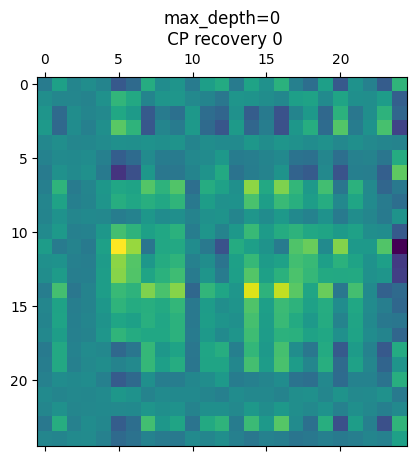
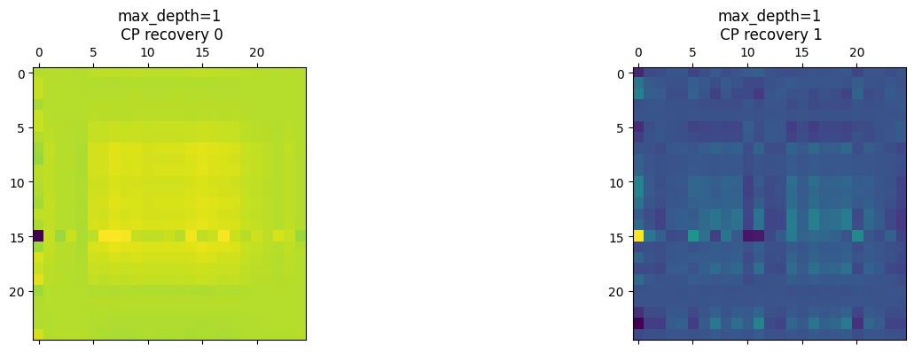
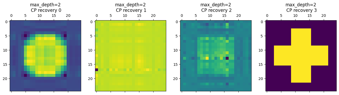
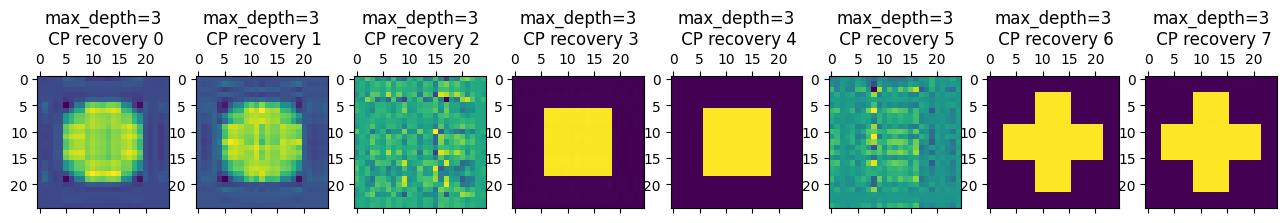
Figure 1: Tensor-input decision tree regression estimated coefficients $\hat{\bm{B}}$ on a mixture-of-classes model ($\tau=0.1$) with rank-2 CP regression at leaf models from the circle-rectangle-cross example in Zhou et al. (2013). Each row corresponds to a max_depth$\in\{0,1,2,3\}$.

The key idea behind the LRE loss is to incorporate low-rank tensor regression as the baseline models on the leaves of a partition tree. Trees can capture non-linear local structures in the underlying mean functions but are ineffective at approximating global smooth structures such as linear patterns on some latent dimensions which low-rank tensor regression targets. As such, we construct trees using novel splitting criteria and complexity measures, then fit tensor regressions at each leaf node. Figure 1 shows a scenario of mixed class data (Zhou et al., 2013) in which existing tensor regressions (i.e., the top row) fail to recover each class but a tree-based regression model is successful with appropriate splits. In addition, this tree-based model can realize typical low-rank CP and Tucker regression models as special cases when the max depth of the tree is set to be zero (i.e., when the tree has only one node) and the only model is a single low-rank regression model. The effects of the splitting criteria will be further investigated in Section 5.1.

 

Result: Train a tensor input single decision tree regressor with exhaustive search

Function fit($\bm{X}\in\mathbb{R}^{n\times d_{1}\times d_{2}}$, $\bm{y}\in\mathbb{R}^{n}$):

begin

       Initialize root node. for node in tree do

             Calculate for all potential splits along each dimension pair $(j_{1},j_{2})$: Find $\arg\min_{j_{0}\in\{1,\cdots,n\},j_{1}\in\{1,\cdots,d_{1}\},j_{2}\in\{1,\cdots,d_{2}\}}LAE(j_{0},j_{1},j_{2})$ or $LRE(j_{0},j_{1},j_{2})$ ;

             With the minimizer $(j_{0}^{*},j_{1}^{*},j_{2}^{*})$, split the dataset on the chosen dimension pair $(j_{1}^{*},j_{2}^{*})$ and split value $\bm{X}[j_{0}^{*},j_{1}^{*},j_{2}^{*}]$, creating left and right child nodes using data in $R_{1},R_{2}$ ;

            

       end for

      Fit the chosen mean/CP/Tucker models at each of the leaf nodes.

end

 

Algorithm 1 Exhaustive search method for fitting tensor input decision tree regressor with low-rank splitting criteria (13) and (14).

2.2 Reducing Computational Cost

There are two major computational overheads in fitting the tree tensor regression model we just proposed: leaf model fitting and splitting criteria computation. The cost of the former is alleviated thanks to the tree structure providing a partitioning regime that allows divide-and-conquer scaling. The latter, however, is a new computational challenge born from the nature of tensor data as we explain below.

It is computationally very expensive to exhaustively search (see Algorithm 1) for the best split node in tensor input decision trees. This process evaluates all possible splits along each dimension pair $(j_{1},j_{2})$, which requires examining every combination of $j_{0}$, $j_{1}$, and $j_{2}$. Consequently, the search space size for each split decision is $n\cdot d_{1}\cdot d_{2}$, which scales poorly with increasing dataset size and tensor dimensions, making exhaustive search computationally intensive and impractical for large-scale data or real-time applications.

In addition, the computational complexity of (13) and (14) is rather high since both CP and Tucker decompositions rely on expensive alternating algorithms, which often have convergence issues. Therefore, the greedy search approach over a space of size $d_{1}d_{2}$ to solve $\min_{(j_{0},j_{1},j_{2})}\mathcal{L}(j_{0},j_{1},j_{2})$ is no longer an efficient algorithmic design, given the frequency of splitting in fitting a regression tree structure.

Splitting criteria complexity analysis.

Computing the variance in (12) using scalar responses has complexity $\mathcal{O}\left(n\right)$, which can be vectorized and does not scale with dimensions. On the other hand, the time complexities of (13) and (14) are dominated by the CP and Tucker low-rank decomposition of the coefficient tensors. Although many scalable methods are proposed for CP and Tucker decompositions, the well-adopted alternating least square (ALS) (Malik and Becker, 2018) solvers are of iterative nature and hence can have relatively high complexities:

Lemma 1.

(CP-ALS per iteration complexity Minster et al. (2023) Section 3.2) In the alternating least square algorithm for the rank-$R$ CP decomposition of a $n\times d_{1}\times d_{2}\times\cdots\times d_{K}$ tensor where $R<n$ and $R\ll d_{i},i=1,\cdots,K$, each iteration has time complexity $\mathcal{O}\left((K+1)\cdot\prod_{i=1}^{K}d_{i}\cdot R\right)$. Therefore, for $N^{*}$ iterations in CP-ALS, the overall complexity is bounded from above by $\mathcal{O}\left(N^{*}\cdot(K+1)R\cdot\left(\max_{i}d_{i}\right)^{K}\right)$.

Lemma 2.

(Tucker-ALS per iteration complexity Oh et al. (2018) Section II.C) In the alternating least square algorithm for the rank-$(R,d_{1}^{{}^{\prime}},d_{2}^{{}^{\prime}},\cdots,d_{K}^{{}^{\prime}})$ (i.e., core tensor dimension) Tucker decomposition of a $n\times d_{1}\times d_{2}\times\cdots\times d_{K}$ tensor, each iteration has complexity

$$\mathcal{O}\left(\min\left\{n\prod_{j=1}^{K}d_{j}^{{}^{\prime}2},n^{2}\prod_{j=1}^{K}d_{j}^{{}^{\prime}}\right\}+\sum_{i=1}^{K}\min\left\{R^{2}\cdot d_{i}\prod_{j\neq i}d_{j}^{{}^{\prime}2},R\cdot d_{i}^{2}\prod_{j\neq i}d_{j}^{{}^{\prime}}\right\}\right).$$

When $R<n$ and $d_{i}^{{}^{\prime}}\asymp d_{i}\ll n,i=1,\cdots,K$, for $N^{*}$ iterations in Tucker-ALS, the overall complexity is at most $\mathcal{O}\left(N^{*}\cdot n\cdot\left(\max_{i}d_{i}\right)^{2K}\right)$.

To simplify our subsequent analysis, we assume $n\asymp R$ and always choose a constant maximal iteration number $N^{*}$ regardless of the convergence. Then both decompositions have time complexities at most $\mathcal{O}\left(N^{*}\cdot n\cdot\left(\max_{i}d_{i}\right)^{2K}\right)$ which scales linearly with $n$. However, the factor $N^{*}\cdot\left(\max_{i}d_{i}\right)^{2K}$ greatly increases complexity in greedy-style tree-fitting, which bottlenecks most regression tree fitting algorithms (Loh, 2014).

Adoption of mean splitting values.

Minimizing these three criteria can be a strategy to choose the split-value index $j_{0}$ and splitting coordinates $(j_{1},j_{2})$, and can easily generalize to regression trees for tensor inputs. Finding the best combination of $(j_{0},j_{1},j_{2})$ using (3), (13), (14), in a worst-case scenario, needs $n\cdot\prod_{j=1}^{K}d_{j}$-many variance evaluations and contributes to a quadratic complexity in $n$. But if we do not optimize over $j_{0}$ and instead split on the sample mean, we can simplify the partitions in (3), (13), (14) as:

$$\bar{R}_{1}\coloneqq\left\{\bm{X}\mid\bm{X}[:,j_{1},j_{2}]\leq\frac{1}{n}\sum_{k=1}^{n}\bm{X}[k,j_{1},j_{2}]\right\},$$ (left child) (16)

$$\bar{R}_{2}\coloneqq\left\{\bm{X}\mid\bm{X}[:,j_{1},j_{2}]>\frac{1}{n}\sum_{k=1}^{n}\bm{X}[k,j_{1},j_{2}]\right\}.$$ (right child) (17)

Since we no longer need to determine $j_{0}$, we can complete the search within linear time in $n$, without losing too much empirical prediction performance. Then the corresponding loss functions in our reduced optimization problems become:

$$\overline{\text{SSE}}(j_{1},j_{2})=\sum_{j=1}^{2}\frac{1}{|I_{j}|}\sum_{\underset{I_{j}=\{k\mid\bm{X}[k,j_{1},j_{2}]\in\bar{R}_{j}\}}{i\in I_{j}}}\left\|\hat{y}_{\bar{R}_{j}}-y_{i}\right\|_{2}^{2},$$ (18)

$$\overline{\text{LAE}}(j_{1},j_{2})=\sum_{j=1}^{2}\sum_{\underset{I_{j}=\{k\mid\bm{X}[k,j_{1},j_{2}]\in\bar{R}_{j}\}}{i\in I_{j}}}\left\|\widetilde{\bm{X}}[i,:,:]-\bm{X}^{(n)}[i,:,:]\right\|_{F}^{2},$$ (19)

$$\overline{\text{LRE}}(j_{1},j_{2})=\sum_{j=1}^{2}\sum_{\underset{I_{j}=\{k\mid\bm{X}[k,j_{1},j_{2}]\in\bar{R}_{j}\}}{i\in I_{j}}}\left\|\widetilde{\bm{y}}\left(\bm{X}^{(n)}[i,:,:]\right)-y_{i}\right\|_{F}^{2}.$$ (20)

This simplification shrinks the dimensionality of the optimization problem $\min_{(j_{0},j_{1},j_{2})}\mathcal{L}(j_{0},j_{1},j_{2})$ to reduce the complexity per evaluation of the split criterion, by removing the search along the first mode.

Figure 2 shows that the loss functions LAE and LRE lead to similar complexities and predictive behavior. Although LAE and LRE are both based on low-rank tensor decomposition, LRE (like SSE) focuses on the children’s predictive loss. In what follows, we mainly study TT models with LRE in (14) or its mean version (20) as our default loss functions, unless otherwise is stated.

Methods of efficient search for splitting coordinates.

Existing efficient methods (Luo and Pratola, 2022; Chickering et al., 2001) for splitting point optimization (i.e., search among possible points for the above loss functions) usually rely on the distribution assumptions on the candidates. In our case, this assumption is usually not realistic due to the complex correlation between dimensions of the input tensor. To reduce the $N^{*}\cdot\left(\max_{i}d_{i}\right)^{K}$ factor further, we propose the following two methods for shrinking the search space of these optimization problems in order to quickly solve the minimization problems for (13) or (14). Both methods have existed in the optimization community for a while and exhibit trade-offs between efficiency and accuracy, but to our best knowledge are applied in regression trees for the first time.

Decision Trees Extra-Trees (ERT) Algorithm 3 Algorithm 4 Reference (Breiman et al., 1984) (Geurts et al., 2006) This paper splitting coordinate Exact optimization Exact optimization Importance sampling Branch-and-bound splitting value Exact optimization Random selection Random $\tau<1$/ Random $\xi>0$/ Exact $\tau=1$ Exact $\xi=0$

Table 1: Comparison of state-of-the-art methods, where we essentially replace the splitting value and coordinate optimization $\min_{(j_{0},j_{1},j_{2})}\mathcal{L}(j_{0},j_{1},j_{2})$ with a surrogate problem and support approximate choices of splitting values to allow more expressive complexity trade-offs.

Leverage score sampling (LS) uses a sample rate $\tau$ to shrink the search space size from $d_{1}d_{2}$ down to $\tau d_{1}d_{2}$ for constrained optimization (see Algorithm 3). When $\tau=1$, LS reduces to exhaustive search. The subset $\mathcal{D}$ of dimension pairs $(j_{1},j_{2})$ is chosen from $\{1,2,...,d_{1}\}\times\{1,2,...,d_{2}\}$ following a LS (without replacement) scheme (Murray et al., 2023; Malik and Becker, 2018). Pairs with higher variance are preferred since they offer diversity and may benefit low-rank approximations for $R_{1},R_{2}$. The probability of choosing a constant-value dimension is zero. LS keeps the same asymptotic computational complexity but sacrifices optimal solutions for faster computation during the greedy search for splits. This per-split strategy also shares the spirit of the traditional $\mathtt{mtry}$-strategy used in random forests (Mentch and Zhou, 2020) which searches $\mathtt{mtry}$ (rather than all) features.

Branch-and-bound optimization (BB) considers a divide-and-conquer strategy for this optimization problem. In Algorithm 4, we introduce the tolerance $\xi$ to divide the search space via the branch-and-bound strategy (Lawler and Wood, 1966; Morrison et al., 2016) and consider the optimization of (13) or (14) within the parameter tolerance $\xi$. When $\xi=0$, this method reduces to regular exhaustive search. BB divides the entire space of $d_{1}d_{2}$ potential splits into smaller search subspaces (i.e., branching). For each subspace, it estimates a bound on the quality of the best split coordinates (minimizing the chosen criterion) that can be found. If this estimated bound is worse than the best split (within the prespecified tolerance $\xi$) found so far, the subspace is excluded from further consideration (i.e., bounding). This method efficiently narrows the search to the most relevant splits and provides a practical alternative to exhaustive search at the price of possible local minima. To support our claim, Figure 2 shows that in the zero-noise cases, both LS and BB tend to have larger MSE compared to exhaustive search, regardless of the choice of leaf node fitting models, and the model quality deterioration becomes severe when the maximal depth increases. When there is more noise (i.e., lower signal-to-noise ratio in data), such differences in MSE between exhaustive search and BB/LS become less obvious. As rank of the leaf model increases, the performance of LS is less stable compared to BB. As the depth of the model increase, BB takes more time to fit compared to the linearly increasing sampling time of LS. Table 1 summarizes the difference between these fast search tree methods.

On one hand, our LS sampling (Algorithm 3) randomly chooses split coordinates but not the splits. It also serves as a surrogate importance measure for each coordinate combination. The LS design of choosing the optimal split among a fraction of all possible splits is related to that of extra-trees (Geurts et al., 2006). Extra-trees differ from classic decision trees in that instead of exhaustively optimizing for the optimal split, random splits are drawn using randomly selected features and the sub-optimal split among those candidates is chosen. When the candidate possible features is 1, this builds a totally random decision tree.

On the other hand, our BB (Algorithm 4) deterministically selects those split coordinates with the best approximation error at a certain tolerance level. BB exhibits a trade-off between the accuracy of the best pair $(j_{1},j_{2})$ minimizing splitting criterion and search complexity but its quality will be affected by the additional tolerance hyper-parameter, which is not always straightforward to tune. BB also generalizes the classical constraint of limiting the maximal number of features used in all possible splits: limiting the number of features restricts the possible partitions induced by the tree, whereas BB also ensures that the “resolution” of tree-induced partition will not exceed a certain tolerance.

In the spirit of Lemma 11 of Luo and Pratola (2022) and the above Lemmas 1 and 2, we can derive the per-iteration complexity (of ALS used for computing CP and Tucker decompositions) by observing that there are $\mathcal{O}(n\log k)$ evaluations of the loss function in a tree with $k$ nodes ($\log k$ layers) and $n\geq 1$ sample points:

Proposition 3.

(Computational complexity for TT) If there are $n\geq 1$ samples with at most $k$ nodes for the splitted tree structure and no more than $N^{*}<\infty$ iterations for all decompositions, the worst-case computational complexity for generating this tree structure (via exhaustive search for problem (15)) is

(1) $\mathcal{O}(nd_{1}d_{2}\log k)$ if the loss function is (12).

(2) $\mathcal{O}(n^{2}d_{1}^{2}d_{2}^{2}\log k)$ if the loss function is (13) or (19) with CP low-rank approximations.

(3) $\mathcal{O}(n^{2}d_{1}^{2}d_{2}^{2}\cdot\left[\min(d_{1}d_{2},n)+\min(d_{1},d_{2})\right]\log k)$ if the loss function is (14) or (20) with Tucker low-rank approximations.

Proof.

See Appendix B. ∎

This complexity result indicates that the tensor tree model has $\mathcal{O}(n^{2}\cdot C)$ complexity (where $C=C(d_{1},d_{2})$ depends on the dimensionality of the tensor inputs) compared to the larger $\mathcal{O}(n^{3})$ complexity (whose constant inside big O also depends on the kernel evaluation) incurred by tensor GP models (Yu et al., 2018) as shown later in Figure 8. We can also see that both LAE and LRE share the same big O complexity in terms of the sample size $n$. As explained in Section 2.1, we will focus on LRE since it parallels the SSE in regular regression trees.

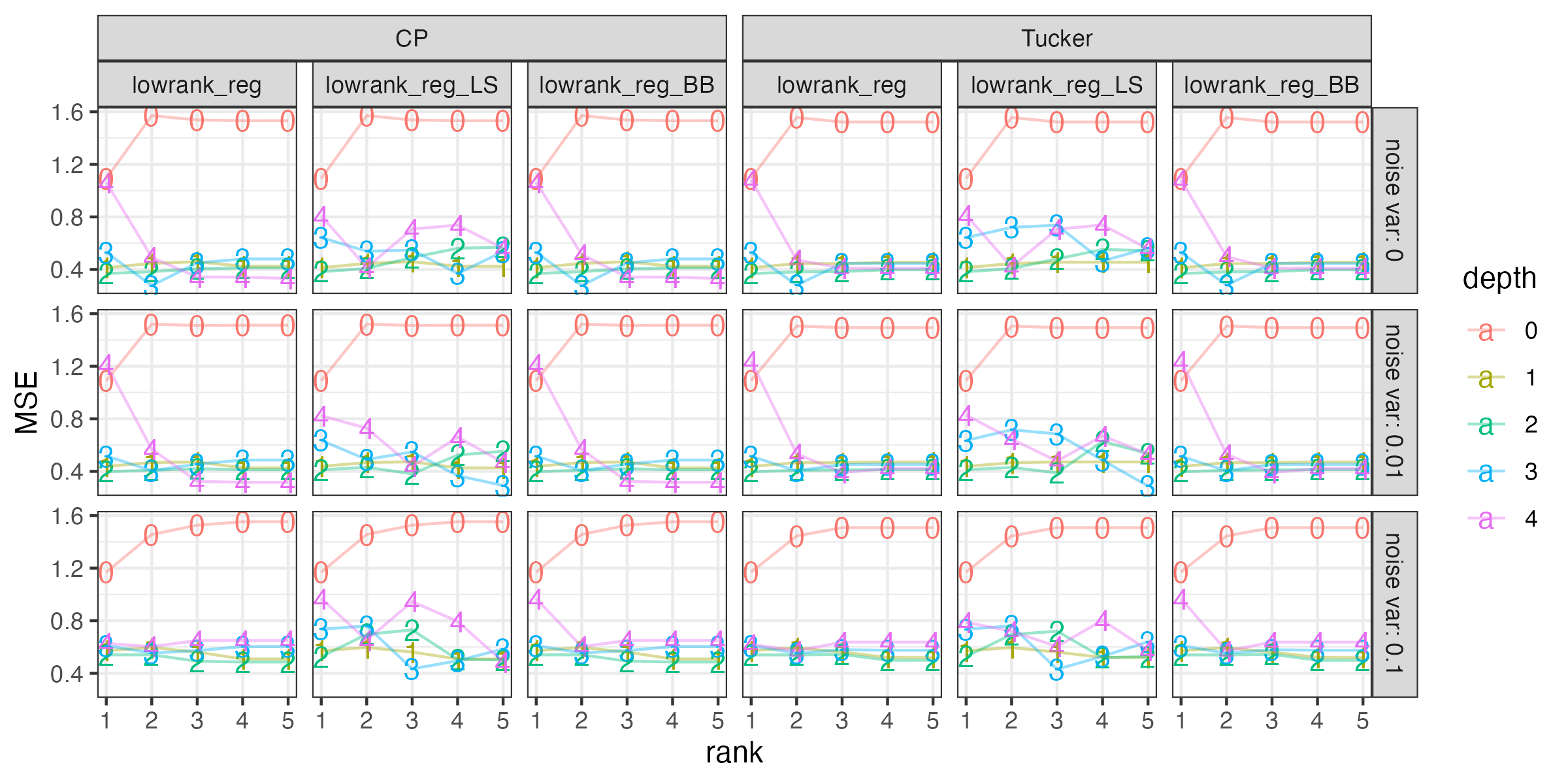
Figure 2: Out-of-sample MSEs for tree regression models of different maximal depths, using a $(500,5,4)$ input tensor $\bm{X}$ sampled uniformly randomly from $[-1,1]$ and scalar output $\bm{y}=2\bm{X}[:,0,1]\cdot\bm{X}[:,2,3]+3\bm{X}[:,1,0]\cdot\bm{X}[:,2,0]\cdot\bm{X}[:,3,0]+\varepsilon$ where $\varepsilon\sim N(0,\sigma^{2})$ and $\sigma^{2}=0,0.01,0.1$. (Columns 1&4: Full search; Columns 2&5: LS with $\tau=0.5$; Columns 3&6: BB with $\delta=0.5$.)

2.3 Complexity-based Pruning

As with traditional tree-based regression methods, pruning and other forms of regularization are necessary to avoid overfitting. Adaptive pruning can be achieved based on a complexity measure $C_{\alpha}(T)$ following the definition in (9.16) in Hastie et al. (2009):

$$C_{\alpha}(T)=\sum_{m=1}^{T}N_{m}Q_{m}(T)+\alpha T_{l},$$ (21)

where $T_{l}$ is the number of leaves in the decision tree, $N_{m}$ is the number of samples in the $m$-th leaf, and $Q_{m}(T)$ is the variance of the response values in the $m$-th leaf. The term $\alpha T_{l}$ introduces a penalty for the tree’s complexity through an apriori user-defined constant $\alpha$. High-bias models oversimplify, resulting in lower variance and smaller $Q_{m}(T)$. More leaves capture details, increasing variance but reducing bias. (21) captures this trade-off by combining both terms, and the parameter $\alpha$ controls the balance between them.

Revisiting the three possible splitting criteria in Section 2.1, we find that variance splitting can correspond naturally to (21). For the low-rank splitting proposed in Algorithm 3, we propose the following modified complexity measure $C_{\text{tl}_{\alpha}}(T)$ which includes a low-rank induced error term $Q_{\text{tl}_{m}}(T)$ and is defined as:

$$C_{\text{tl}_{\alpha}}(T)=\sum_{m=1}^{T}N_{m}Q_{\text{tl}_{m}}(T)+\alpha T_{l}$$ (22)

The measure $C_{\text{tl}_{\alpha}}$ generalizes $C_{\alpha}$ by accounting for the structure and relationships in multi-dimensional data. The term $Q_{m}(T)$ in (21) is replaced by $Q_{\text{tl}_{m}}(T)$, which can be chosen as one of (3), (13) or (14) to evaluate the fitness of the leaf models given a tree structure $\mathcal{T}$ (i.e., bias component). This captures the inherent complexity in tensor data and reflects how well the model fits the underlying tensor structure. The variance term remains the same, representing the complexity of the tree through the number of leaves.

By considering the low-rank prediction errors, the measure $C_{\text{tl}_{\alpha}}$ (as discussed in Hastie et al. (2009)) also balances the trade-off between fitting the tensor structure (the first summation term in (22) as bias) and the complexity of the decision tree (the second summation term in (22) as variance). The trade-off between bias and variance also happens when we fit tensor regression models at each leaf. This makes our model suitable for multi-dimensional data. Both $C_{\alpha}$ and $C_{\text{tl}_{\alpha}}$ provide a way to prune the tree $\mathcal{T}$ and maintain a simple model (high bias, low variance), which is essential for achieving good generalization performance.

In our TT models, we implement recursive pruning (without swapping or other kinds of reduction operations, for simplicity) based on whether a specific branch will reduce complexity. When we compute the first term in (22) (the second term will be affected by the choice of $\alpha$) we can observe that a deeper tree may not necessarily improve the overall fit. We can also see that (21) is no longer a suitable complexity measure when we use tensor leaf node models $m_{j}$ since these models are fitting the subdatasets at each leaf node well. Dividing the dataset into more subsets will reduce the variance in each leaf node but the overall prediction errors actually increase, reflected by the increasing first term in (22).

Pruning is needed to get a good fit and prediction in a tensor input tree regression model. We may adjust $\alpha$ in the term $\alpha T_{l}$ to favor shallower trees. However, if we use $\sum_{m=1}^{T}N_{m}Q_{\text{tl}_{m}}(T)$ in (22) to guide our pruning, the depth of the tree tensor model should be 0; if we use $\sum_{m=1}^{T}N_{m}Q_{m}(T)$ in (21) to guide our pruning, the depth of the tree tensor model should be 1. Corresponding to these two choices, it is clear that the predictive error is better when there is no splitting at all.

We show the effect of pruning using the following tensor-input scalar-output synthetic function

$$f(\bm{X})=\begin{cases}5&\text{if }\bm{X}[:,0,1,0]\geq 0.4\\ -1&\text{if }\bm{X}[:,0,1,0]<0.4\text{ and }\bm{X}[:,2,2,0]\geq 0.65\\ -4&\text{otherwise}\end{cases}.$$ (23)

Hence the function can be represented by a tree with three leaves. As shown in Figure 3, we fit trees using the variance splitting criterion and various pruning parameter values $\alpha$. First we observed that for all shown $\alpha$ values that the MSE decreases with tree’s maximal depth, and that this decrease levels off once the maximal depth is two or larger. We also see that trees under $\alpha=0$ (i.e., without pruning) can grow to have many leaves, but once pruning is introduced ($\alpha>0$), trees with $\texttt{maxdepth}\geq 2$ are typically pruned to have three or four leaves, especially at $\alpha=0.1$ (i.e., the largest tested $\alpha$ value). Hence, in this example, an appropriately large $\alpha$ value induces sufficient pruning for trees to have the “correct” number of leaves.

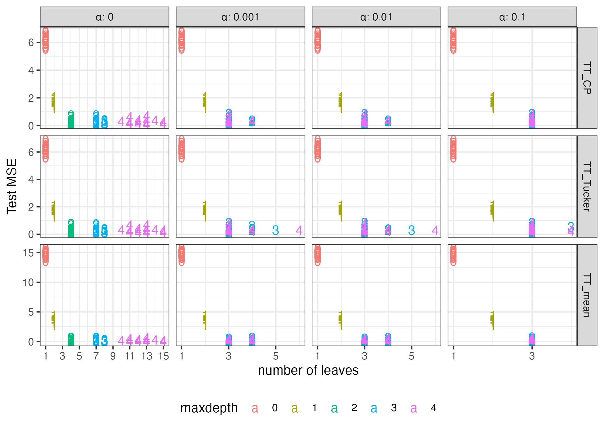
Figure 3: Out-of-sample MSE of trees trained on data generated by first sampling $(500,4,4,4)$ input tensor $\bm{X}$ uniformly randomly from $[0,1]$ and then evaluating the function (23) at the input tensor before adding i.i.d. Gaussian noise with mean zero and variance $0.1$. The figure shows 20 replicates for each combination of $\alpha$, maxdepth, and leaf model.

2.4 Summary of Single Tensor Tree Model

We can summarize our model construction for efficient tensor tree (TT) models for tensor input $\bm{X}\in\mathbb{R}^{n\times d_{1}\times d_{2}}$, where $n$ is the number of observations, and $d_{1},d_{2}$ are the tensor’s dimensions, and scalar response $\bm{y}\in\mathbb{R}^{n}$. Our single tree models assume a tree structure $\mathcal{T}$; at the leaf nodes we propose to fit low-rank scalar-on-tensor regression CP/Tucker models (Zhou et al., 2013; Li et al., 2018) to adapt to low-rank structures in tensors. This is a direct but novel generalization to non-linear tree models (Chaudhuri et al., 1994; Li et al., 2000) onto non-standard tensor-input domains, and also a natural generalization of low-rank tensor models to handle heterogeneity.

In tensor regression trees, the splitting criterion involves entire tensor dimensions, and the decision to split is based on a low-rank approximation criterion, either $\text{LAE}(j_{0},j_{1},j_{2}),\overline{\text{LAE}}(j_{1},j_{2})$ or $\text{LRE}(j_{0},j_{1},j_{2}),\overline{\text{LRE}}(j_{1},j_{2})$. This consideration makes the splits more nuanced. Traditional decision trees evaluate splits based on single features, but tensor regression trees consider interactions between multiple dimensions, adding computational complexity. The enhanced complexity and the higher number of potential decision boundaries with tensors increase the risk of overfitting, which makes regularization via pruning essential. As we transition to tensor regression trees, interpretability can become a challenge due to intricate decision boundaries. Lastly, operations like low-rank approximations can be computationally intensive, requiring efficient algorithms or specialized hardware. Therefore, we further tackle the scalability problems that arise in tensor regression settings (Kolda and Sun, 2008; Liu, 2017) with the following innovations.

1. We propose criteria (18), (19) and (20) to split the tree structure $\mathcal{T}$, which reduces the dimensionality of the optimization problem $\min_{(j_{0},j_{1},j_{2})}\mathcal{L}(j_{0},j_{1},j_{2})$.

2. We propose randomized and branch-and-bound optimization methods (i.e., LS and BB) , which trades the accuracy of the optimization problem $\min_{(j_{0},j_{1},j_{2})}\mathcal{L}(j_{0},j_{1},j_{2})$ for better complexity.

3. We generalize complexity measures into (22) using new criteria for tree pruning, which achieves parsimonious partition structures.

The first and third adjustments allows us to attain a flexible divide-and-conquer for model aggregation regime within a tree. The second adjustment essentially introduces randomness into the tree splitting procedure (i.e., LS) or trades optimization quality for scalability (i.e., BB) for efficiency in tree structure search. Figure 1 shows that our tree model can adapt to potentially heterogeneous datasets and hence benefits from flexible structures.

3 Ensemble of Trees

Continuing our discussion of TT models in Section 2.4, a single tree model tends to have large variance and overfit the data, which can produce inconsistent predictions. The idea behind tree ensemble modeling is to combine multiple models in order to improve the performance of a single TT model. Ensemble methods are foundational in modern machine learning due to their effectiveness in improving predictive performance. We first describe a boosted TT ensemble, then use it to fit a tensor response regression model.

3.1 Boosted Trees

Before describing boosted trees in detail, we first introduce a different tree ensemble method called Random Forests (RFs). Random Forests (Breiman, 2001; Amit and Geman, 1997) create an ensemble of independent decision trees using bootstrap samples and random feature subsets, enhancing diversity and robustness through randomization over the feature space. For a given set of $n$ data pairs $(\bm{X}_{i},y_{i})$, where $\bm{X}_{i}$ are input tensors and $y_{i}$ are scalar responses, a RF builds $B$ trees. Each tree is trained on a bootstrap sample of the data, and at each split, a random subset of features is considered as shown in Algorithm 5. This approach reduces the variance of the model by averaging the predictions of independently trained trees, which helps mitigate overfitting. The main challenge of ensembling trees is ensuring that the trees are diverse enough to capture different patterns in the data without making inconsistent predictions.

Although RFs combined with TT (See Algorithm 5) are powerful, its performance on predicting entries in a tensor output is not ideal. We focus on boosting methods, which iteratively improve the model by focusing on previously mispredicted instances. Boosting constructs trees sequentially, where each new tree corrects errors from the previous ones, leading to a strong aggregated model. Therefore, the concept behind boosting diverges fundamentally from RF. Boosting does not aggregate weak learners; instead, it averages the predictions of strong learners. This method is particularly effective for our tensor regression tree models, as detailed in the following sections. Gradient Boosting (Friedman, 2001) constructs an ensemble of decision trees sequentially, where each new tree is trained to correct the errors of the existing ensemble. Unlike RFs, where trees are built independently, GB involves a functional gradient descent approach to minimize a specified loss function (Hastie et al., 2009).

In the general case, gradient boosting involves computing “pseudo-residuals,” which are the negative gradients of the loss function with respect to the model’s predictions. For a given loss function $L(y,F(\bm{X}))$, the pseudo-residuals at iteration $b$ are given by:

$$r_{i}^{(b)}=-\left[\frac{\partial L(y_{i},F(\bm{X}_{i}))}{\partial F(\bm{X}_{i})}\right]_{F(\bm{X})=F_{\text{GB}}^{(b-1)}(\bm{X})}.$$

Each new tree $g_{b}$ is then fit to these pseudo-residuals, and the model is updated as follows:

$$F_{\text{GB}}^{(b)}(\bm{X})=F_{\text{GB}}^{(b-1)}(\bm{X})+\eta g_{b}(\bm{X};T_{b},M_{b}),$$

where $\eta$ is a learning rate that controls the contribution of each tree. The new tree minimizes the loss function:

$$\text{argmin}_{T_{b},M_{b}}\sum_{i=1}^{n}L\left(y_{i},F_{\text{GB}}^{(b-1)}(\bm{X}_{i})+g_{b}(\bm{X}_{i};T_{b},M_{b})\right).$$

In our case, we focus on a simpler version of tree boosting algorithm, which uses the squared error loss (for the scalar response $y$). This approach iteratively fits trees to the residuals of the previous trees without explicitly computing pseudo-residuals. For a set of $n$ data pairs $(\bm{X}_{i},y_{i})$, one popular tree boosting model constructs an additive series of $m$ regression trees:

$$F_{\text{GB}}(\bm{X})=\sum_{b=1}^{m}g_{b}(\bm{X};T_{b},M_{b}),$$ (24)

where each tree $g_{b}(\bm{X};T_{b},M_{b})$ is fit to the residuals of the previous ensemble:

$$r_{i}^{(b)}=y_{i}-F_{\text{GB}}^{(b-1)}(\bm{X}_{i}).$$ (25)

Each new tree is trained to minimize the squared error loss on these residuals:

$$\text{argmin}_{T_{b},M_{b}}\sum_{i=1}^{n}\left(r_{i}^{(b)}-g_{b}(\bm{X}_{i};T_{b},M_{b})\right)^{2}.$$

By sequentially fitting trees to the residuals, the forward-stagewise fitting approach builds a strong aggregated model, effectively capturing the complex patterns in the data while mitigating overfitting. This method is particularly suitable for our tensor regression tree models, as detailed in the following sections.

In the context of tensor regressions, gradient boosting is particularly powerful. Each tree corrects the residuals of the previous ensemble, enabling the model to capture complex patterns in multi-dimensional data, which is crucial for tensor inputs and outputs. GB can also incorporate regularization, such as shrinkage and tree constraints, to prevent overfitting, which is vital when modeling high-dimensional tensor data. Our current approach does not include regularization in the ensemble. CatBoost (Prokhorenkova et al., 2018) and XGBoost (Chen and Guestrin, 2016) are notable implementations of regularized gradient boosting that offer enhanced performance for input vectors with number of modes $K=1,2$. Converting tensor inputs to tabular form (i.e., $K=1,2$) typically involves flattening, which can lead to loss of spatial or sequential information. Boosting algorithms iteratively build decision trees, and the complexity of constructing trees grows with the dimensionality of the input space. Tensor inputs significantly increase the dimensionality, making tree construction inefficient and potentially leading to overfitting (CatBoost does not allow pruning) or redundant splits over the flattening space. Our implementation generalizes to $K>2$ without regularization.

Algorithm 6 combines gradient boosting and adaptive sampling with the multi-dimensional prowess of tensor regression trees in order to achieve highly accurate predictive models that are especially suited for complex, multi-dimensional datasets. We will be able to combine $m$ different weak learners in a residualized back-fitting scheme, and choose a learning rate (which is usually greater than $1/m$) that allows the aggregated model to leverage the prediction power. From our experience, the GB is more appropriate than RF and yields more significant improvement in model prediction power, and we will focus on GB in the rest of the text. Our software simultaneously supports both gradient boosting (Chen and Guestrin, 2016) and AdaBoost.R2 (Drucker, 1997) as two special cases of the arcing (perturb and combine) technique (Breiman, 1999) that are used widely in tree ensemble regressions.

3.2 Tensor-on-tensor: Multi-way Output Tensor Trees via Ensemble

We now consider a regression problem for tensor inputs $\bm{X}_{i}\in\mathbb{R}^{d_{1}\times d_{2}}$ and tensor responses $\bm{y}_{i}\in\mathbb{R}^{p_{1}\times p_{2}}$. We focus on this special case but emphasize that this result can be extended to higher order tensors:

$$\bm{y}_{i}=\bm{g}^{*}(\bm{X}_{i})+\bm{E}_{i},i=1,\ldots,n.$$ (26)

Here $\bm{g}^{*}\colon\mathbb{R}^{d_{1}\times d_{2}}\rightarrow\mathbb{R}^{p_{1},p_{2}}$ is a tensor-valued function and the $\bm{E}_{i}$s are independent mean zero noises.

Lock (2018) proposes to treat a linear tensor-on-tensor regression problem. For tensor output $\bm{y}\in\mathbb{R}^{n\times p_{1}\times p_{2}}$ (we again emphasize that this result can be extended to higher order tensors), their methodology performs optimization directly on $\|\bm{y}-\bm{X}\circ\bm{B}\|_{F}$ with an optional regularization term penalizing the tensor rank of the coefficient tensor $\bm{B}$. A naive approach is to replace the linear scalar-on-tensor regression model at the leaf node with a tensor-on-tensor regression model so that the tree naturally adapts to the tensor output for each node fitting and prediction, which is supported by our implementation by replacing CP/Tucker models with tensor-on-tensor models. The issue with this naive approach is that tensor-on-tensor regression is a very high-dimensional problem and very sensitive to pruning.

Instead, we propose two alternative approaches for TT models based on ensemble modeling using tree regressions (Breiman et al., 1984; Breiman, 2001). From the previous section, we know that GB can improve the predictive power of a single tree; in what follows, we will use pruning parameter $\alpha=0.1$ and $10$ single trees for each GB ensemble unless otherwise stated. We can also use other ensemble methods (e.g., RF, Adaboost (Breiman, 1999)) or even different kinds of ensembles for different entries (in entrywise approach) or components (in lowrank approach). As mentioned earlier, we will focus on “ensemble of GBs”:

1. Entry-wise approach. The first approach (TTentrywise-CP, TTentrywise-Tucker) is to use a single GB ensemble to predict vector slices $\bm{y}[:,i,j],i=1,\cdots,p_{1};j=1,\cdots,p_{2}$ of the tensor output as if the slices are mutually independent, which facilitates parallel computation but ignores the dependence between slices. However, this trades the loss of dependency with improved computational cost since the break-down into $p_{1}\times p_{2}$ single TT trees and the overall complexity is scaled up by a factor of $\mathcal{O}(p_{1}\times p_{2})$. This method is prone to overfitting but is not sensitive to the rank choice.

2. Low-rank approach. The second approach (TTlowrank-CP, TTlowrank-Tucker) is to perform CP/Tucker decomposition on the tensor output $\bm{y}$ and use a single GB ensemble to predict each component (i.e., $\mathbf{a}_{r},\mathbf{b}_{r},\mathbf{c}_{r}$ in (7); $\bm{A}_{1},\bm{A}_{2},\bm{A}_{3}$ in (8)) in the low-rank decomposition. The low-rank decompositions align tensor structures but can be computationally intensive (the cost of decomposing $\bm{y}$ can be obtained by directly applying Lemmas 1 and 2), especially when leaf nodes contain fewer samples than the selected rank of the decomposition which may not be enough to ensure a reasonable fit and generalization ability. This approach allows parallelism only within each component as matrices. In addition to the higher dimensionality, evaluating tensor gradients puts additional computational burden for this direct generalization. This approach allows us to break down the regressions into vector components for fitting using single trees and the overall complexity is scaled up by these factors that is dependent on the ranks we choose for CP or Tucker decompositions.

The entry-wise approach TTentrywise naïvely ignores the tensor structure in $\bm{y}$ and simply flattens it into a vector form. Therefore, this can easily overfit the training set across output entries. When the data has large signal-to-noise ratio, this approach usually works well even when evaluating on testing data. This naive approach of using tensor-on-tensor models at leaf nodes assumes independence between data across leaf nodes; the TTentrywise approach assumes independence between entries of the output tensor, and works well when the elements of the output tensor have minimal or no correlation.

The low-rank approach TTlowrank performs CP or Tucker decomposition on the response to offer a low-rank representation to handle multi-dimensional data by leveraging the structures and relationships within tensor outputs. By decomposing the output tensor into a lower-dimensional form and using the result as features, we enable powerful regression models that can capture complex patterns in the data. We perform a low-rank decomposition and record weights (if CP) or core tensor (if Tucker) but fit our TT regressions on the factors. Then on a new input $\bm{X}$, we predict the corresponding factors and reconstruct the tensor output predictions using the recorded weights (if CP) or core tensor (if Tucker).

Intuitively, CP decomposition preserves the potential diagonality, while Tucker decomposition preserves the potential orthogonality in the output tensor. This approach is suitable when the elements of the output tensor are correlated and exhibit complex relationships, and yield much smaller models compared to the naive approach. Specifically, if we treat matrix outputs as 2-way tensors, then this approach is like performing regressions on the eigenvectors of the decomposed matrix outputs. Mathematically, neither the number of modes nor the assumed rank for the decomposition of the tensor output $\bm{y}$ need to match that of the input $\bm{X}$ nor the target ranks of tensor regression models at the leaves, but we find that setting the decomposition rank equal to the regression rank often works well.

Here we empirically compare the predictive performance of Lock (2018)’s approach with that of our two TT approaches. To generate our datasets, we randomly sample entries of $\bm{X}$ using a uniform distribution on $[0,1]$ and compute $\bm{y}$ using the functions listed in Table 2 (whose ranges are all within $[-1,2]$), and add a uniform noise of scale 0.01. The training and testing sets are generated independently; all models are fitted on the training set, and the predictive performance is evaluated on only the testing set. For rrr methods (Lock, 2018), we set the $\mathtt{R}$ rank parameter and leave the remaining parameters as the package default. For TT methods, we set both splitting ranks and regression ranks to be the same as $\mathtt{R}$, with max_depth =3 and pruning measures $\alpha=0.01$. We use a GB ensemble with 10 estimators and learning rate 0.1 uniformly.

	$(d_{1},d_{2})$	dim $y$	Function expressions
Linear	(3,4)	15	$\bm{y}[:,i]=\begin{cases}\bm{X}[:,0,1]+\bm{X}[:,1,1]&\text{if }i\mod 3=0\\ \bm{X}[:,1,1]+\bm{X}[:,2,0]&\text{if }i\mod 3=1\\ \bm{X}[:,2,2]+\bm{X}[:,0,3]&\text{if }i\mod 3=2\end{cases}$
Non-linear	(3,4)	6	$\bm{y}[:,i]=\sin(\bm{X}[:,i\mod 3,i\mod 4])$
Exact CP (4)	(12,6)	7	$\bm{y}[:,i]=\tilde{\bm{X}}[:,0,1]^{2}-\bm{X}[:,0,0]$ ()
Exact Tucker (4, 4, 4)	(12,6)	7	$\bm{y}[:,i]=\tilde{\bm{X}}[:,0,1]^{2}-\bm{X}[:,0,0]$ ()

Table 2: Information about each simulation in Table 3.

Table 3 shows the out-of-sample errors of each model, where we see that at least one of the TT methods either ties or outperforms both rrr methods in 23 of the 24 tested scenarios. The comparison can be separated into two groups. One group (Linear/Non-linear) explores the power of using GB ensemble TT models (with pruning) along with the two approaches for tensor-on-tensor regression tasks (here for simplicity we choose the same regression rank $R$ for CP models or $(R,R,R)$ for Tucker models for both input $\bm{X}$ and output $\bm{y}$). Using the RPE metric, we can observe that TT with GB for tensor output performs quite competitively with the rrr models and improves as the low-rank models’ rank increases, and only TT model can possibly capture non-linear interactions as expected. This is intuitive since a higher decomposition rank on the output tensor $\bm{y}$ means a better approximation to the tensor-output. In the TTlowrank method with Tucker decomposition on $\bm{y}$, the Tucker decomposition is behaving very badly regardless of ranks and shows non-convergence after max_iters, since the components in $\bm{y}$ possess high correlations. This partially explains why its RPE is greater than 1 for the linear and non-linear examples, and its performance is the worst for this group due to the fact that we do not assume low-rank structure in the output $\bm{y}$ (see Table 2). It seems that the practice of using rank $(R,R,R)$ for Tucker decomposition on $\bm{y}$ does not reflect the tensor structure in the output well in this group of experiments.

In the linear and non-linear signal scenarios, the lowest RPE values are generally associated with the rrrBayes and TTlowrank_CP methods, which are pretty close to the rrr methods as expected. These two examples suggest that our tree-based tensor regression methods become more efficient as rank increases since the approximation quality improves.

The second group of experiments (Exact CP/Exact Tucker) considers the case where there are essentially non-trivial TT trees (with pruning) in GB ensembles. Setting max_depth$>$0 allows a localization effect on the data induced by the partitioning of the tree structures, which allows us to capture behaviors (e.g., periodic) in each weak learner. The TTentrywise and TTlowrank approaches work quite well with CP decomposition, suggesting again quite competitive performance against rrr models. The Tucker decomposition still seems to suffer from the $(R,R,R)$ rank prescription, which leads to occasional non-convergence warnings (raised by $\mathtt{tensorly}$, and we will re-run such experiments to ensure converged results). In the Exact CP and Exact Tucker examples, the signals depend only on the low-rank reconstructed $\bm{X}$ and therefore shall favor TT models with correct ranks $R$.

Interestingly, the TT models do not seem to benefit much when $R$ is correctly specified. We believe that this is due to the fact that the additive noise on $\bm{y}$ makes it not exactly low-rank, but numerically low-rank. In this case, a regularization term in output approximation (like rrr) will help to stabilize the model predictions. In the Exact CP (4) scenario, TTlowrank_Tucker consistently outperforms the other methods across all ranks. This demonstrates the robustness of TTlowrank_Tucker in capturing the underlying structure of this tensor type, which aligns with the CP decomposition. In the Exact Tucker (4, 4, 4) scenario, TTlowrank_Tucker achieves the lowest RPE at ranks 2 to 7. This suggests that the underlying tensor structure may benefit from different decompositions depending on the rank, yet the optimal model rank does not match the underlying true rank used for reconstructing the $\bm{X}$ tensor.

Rank	rrr	rrrBayes	TTentrywise_CP	TTentrywise_Tucker	TTlowrank_CP	TTlowrank_Tucker
2	143 ± 9	136 ± 9	218 ± 3	223 ± 4	172 ± 2	3581 ± 79
3	172 ± 9	162 ± 7	219 ± 3	219 ± 3	132 ± 2	3633 ± 84
4	177 ± 10	171 ± 9	219 ± 3	219 ± 3	134 ± 2	3678 ± 90
5	178 ± 5	170 ± 5	216 ± 3	216 ± 3	133 ± 2	3628 ± 92
6	174 ± 7	207 ± 24	219 ± 4	219 ± 4	137 ± 2	3715 ± 106
7	260 ± 17	319 ± 24	219 ± 3	219 ± 3	138 ± 2	3659 ± 85

(a) Linear

Rank	rrr	rrrBayes	TTentrywise_CP	TTentrywise_Tucker	TTlowrank_CP	TTlowrank_Tucker
2	219 ± 5	209 ± 3	205 ± 2	206 ± 3	297 ± 2	1249 ± 18
3	231 ± 8	211 ± 4	205 ± 2	206 ± 3	260 ± 2	1265 ± 25
4	240 ± 9	218 ± 6	205 ± 2	206 ± 3	231 ± 3	1290 ± 27
5	241 ± 11	222 ± 8	205 ± 2	206 ± 3	200 ± 2	1279 ± 12
6	257 ± 8	240 ± 8	203 ± 2	204 ± 2	169 ± 2	1328 ± 23
7	288 ± 31	276 ± 32	205 ± 2	206 ± 3	261 ± 34	1332 ± 38

(b) Non-linear

Rank	rrr	rrrBayes	TTentrywise_CP	TTentrywise_Tucker	TTlowrank_CP	TTlowrank_Tucker
2	342 ± 69	326 ± 65	455 ± 36	464 ± 35	392 ± 43	204 ± 37
3	433 ± 91	404 ± 86	456 ± 36	465 ± 34	395 ± 42	204 ± 37
4	531 ± 106	490 ± 97	456 ± 36	466 ± 34	398 ± 42	205 ± 38
5	609 ± 115	553 ± 107	456 ± 36	468 ± 34	400 ± 42	204 ± 37
6	666 ± 127	596 ± 117	456 ± 36	468 ± 34	403 ± 42	206 ± 38
7	666 ± 127	596 ± 117	456 ± 36	468 ± 34	406 ± 42	205 ± 38

(c) Exact CP (4)

Rank	rrr	rrrBayes	TTentrywise_CP	TTentrywise_Tucker	TTlowrank_CP	TTlowrank_Tucker
2	376 ± 114	335 ± 98	452 ± 42	463 ± 41	395 ± 47	208 ± 57
3	480 ± 134	427 ± 122	451 ± 41	464 ± 42	395 ± 46	208 ± 57
4	537 ± 153	491 ± 141	451 ± 41	464 ± 42	397 ± 46	209 ± 57
5	609 ± 177	545 ± 153	451 ± 41	464 ± 42	400 ± 46	206 ± 56
6	668 ± 189	591 ± 166	451 ± 41	464 ± 42	403 ± 46	206 ± 56
7	668 ± 189	591 ± 166	451 ± 41	464 ± 42	406 ± 46	209 ± 57

(d) Exact Tucker (4, 4, 4)

Table 3: Out-of-sample RPE (multiplied by 1000 to highlight decimal differences) of various tensor-output regression models trained on the synthetic data described in Table 2. Bold font indicates the smallest RPE of a given rank and signal; we use $\pm$ to represent the standard error of each metric over 10 repeats.

3.3 Summary of Tensor Tree Ensembles

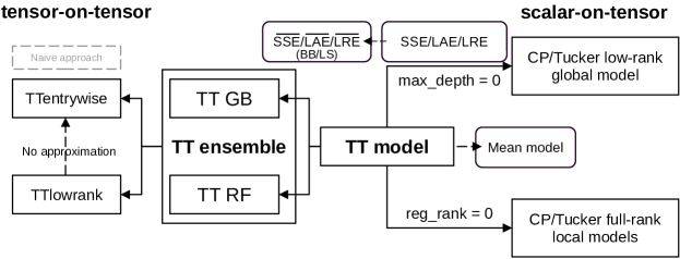
Figure 4: Design summary of the TT models (scalar-on-tensor) and ensembles (tensor-on-tensor).

Boosting methods like GB employ functional gradient descent to minimize a specified loss function. The process involves calculating pseudo-residuals, fitting new trees to these residuals, and updating the model iteratively. This GB along with TT method is favored over random forests and particularly effective for tensor regression tree models, capturing complex patterns in multi-dimensional output.

To addresses multi-way regression problems by performing optimization directly on tensor outputs, we deploy GB ensemble of TT along with two alternative approaches for tensor regression trees (TT models) using ensemble methods:

1. Entry-wise Approach (TTentrywise-CP, TTentrywise-Tucker): This approach predicts vector slices of the tensor output independently, facilitating parallel computation. It trades the loss of dependency between slices for improved computational cost. Although prone to overfitting, this method is not sensitive to rank choice since it does not need decomposition on $\bm{y}$.

2. Low-rank Approach (TTlowrank-CP, TTlowrank-Tucker): This approach performs CP/Tucker decomposition on the tensor output, aligning tensor structures in $\bm{y}$ while being realatively computationally intensive. It predicts decomposed components and reconstructs the tensor output, preserving potential diagonality (CP) or orthogonality (Tucker).

Figure 4 illustrates how we construct ensemble models and how GB (or RF) ensemble of TT models can be utilized to perform tensor-on-tensor regressions. Ensemble methods, in particular boosting, are adopted for tensor output regressions for their ability to sequentially improve models by focusing on residuals, making them suitable for complex tensor-on-tensor regression tasks.

4 Theoretical Guarantees

Although this paper focuses on developing new modeling methodologies and fast training algorithms, we use existing theoretical results to support the validity of our modeling designs. The results in this section all assume scalar responses.

4.1 Coefficient Asymptotics

A fixed tree of depth $K$ has at most $2^{K}$ leaf nodes. In the recursive partition literature (e.g., (2.27) in Gordon and Olshen (1978)), it is commonly assumed that for each leaf node $t$, the number of samples $n_{t}$ tends to infinity when the overall sample size $n$ tends to infinity. This condition obviously holds when we split on the median in the vector input case, but is not necessarily true if we split according to (10), (11) or (16), (17). Under this assumption, within each leaf node we can directly apply existing coefficient estimate consistency results for CP and Tucker regression models (Zhou et al., 2013; Li et al., 2018).

Proposition 4.

For a fixed complete binary tree of depth $K<\infty$, assume for each leaf node $t$ that the number of i.i.d. samples $n_{t}\rightarrow\infty$ and the leaf model parameter space is compact.

(a) (Theorem 1 in Section 4.3 of Zhou et al. (2013)) For the leaf node CP model $y_{i}=\bm{X}[i,:,:]\circ\bm{B}_{0}(t)+E_{i}$ with mean-zero normal error and $\bm{X}[i,:,:]\in R_{t}$, suppose the true coefficient $\bm{B}_{0}(t)=\sum_{r=1}^{R}\lambda_{r}(t)\mathbf{a}_{r}(t)\times\mathbf{b}_{r}(t)\times\mathbf{c}_{r}(t)$ of node $t$ is identifiable up to permutation in the sense of Proposition 4 in Zhou et al. (2013). Then the MLE $\hat{\bm{B}}_{n}(t)$ converges to $\bm{B}_{0}(t)$ in probability.

(b) (Theorem 1 in Section 4.3 of Li et al. (2018)) For the leaf node Tucker model $y_{i}=\bm{X}[i,:,:]\circ\bm{B}_{0}(t)+E_{i}$ with mean-zero normal error and $\bm{X}[i,:,:]\in R_{t}$, suppose the true coefficient $\bm{B}_{0}(t)=\mathbf{G}(t)\times_{1}\mathbf{A}_{1}(t)\times_{2}\mathbf{A}_{2}(t)\times_{3}\mathbf{A}_{3}(t)$ of node $t$ is identifiable up to permutation in the sense of Proposition 3 in Li et al. (2018). Then the MLE $\hat{\bm{B}}_{n}(t)$ converges to $\bm{B}_{0}(t)$ in probability.

Though often presupposed, the condition $n_{t}\rightarrow\infty$ assumes fixed tree and leaf node partitions $R_{t}$, which is not realistic since typically the partition changes as $n\rightarrow\infty$. It also requires an additive underlying true function $f(\bm{X})=\sum_{t\text{ is a leaf node}}\bm{X}\circ\bm{B}_{0}(t)\cdot\bm{1}\left(\bm{X}\in R_{t}\right)$ whose summands are piece-wise multilinear functions. Furthermore, even under these restrictions we still do not have estimates for the ranks of tensor coefficients, as pointed out by Zhou et al. (2013) and Li et al. (2018). However, Proposition 4 confirms one important aspect that if $f(\bm{X})=\bm{X}\circ\bm{B}_{0}$ for some global $\bm{B}_{0}$ (for CP or Tucker model), our tree model produces consistent coefficient estimates for arbitrary (hence dynamic) partitions, since

$$\bm{X}\circ\bm{B}_{0}=\bm{X}\circ\bm{B}_{0}\cdot\left\{\sum_{t\text{ is a leaf node}}\bm{1}\left(\bm{X}\in R_{t}\right)\right\}=\sum_{t\text{ is a leaf node}}\bm{X}\circ\bm{B}_{0}\cdot\bm{1}\left(\bm{X}\in R_{t}\right)$$ (27)

and $\bm{B}_{0}=\bm{B}_{0}(t)$. With this positive result, our tensor tree model for any maximum depth $K$ is no worse than the standalone CP or Tucker model in terms of consistency under $f(\bm{X})=\bm{X}\circ\bm{B}_{0}$.

Moving on to dynamic binary trees, we can establish asymptotic results following the idea of fitting a piece-wise polynomial per partition (Chaudhuri et al., 1994; Loh, 2014). However, Theorem 1 in Chaudhuri et al. (1994) cannot directly apply because the tensor regressions are not analytically solved (i.e., for tensor regression models, the MLE $\hat{\bm{B}}_{n}$ of the regression coefficient does not have an analytic solution).

4.2 Oracle Error Bounds for (12)

As seen above, the fitted mean function from a decision tree regression model lies in the additive class with iterative summation across tensor dimensions $d_{1},d_{2}$:

$$\mathcal{G}^{1}\coloneqq\left\{g\colon\mathbb{R}^{d_{1}\times d_{2}}\rightarrow\mathbb{R}\middle|\ g(\bm{X})=\sum_{i_{2}=1}^{d_{2}}\sum_{i_{1}=1}^{d_{1}}g_{i_{1},i_{2}}(\bm{X}[i_{1},i_{2}])\right\},$$ (28)

which is essentially the same functional class as that in Klusowski and Tian (2024) but with both dimensions additively separable. Within this class, a more useful result regarding the prediction risk can be established, which works for both fixed trees and dynamically splitting trees.

Theorem 5.

(Empirical bounds for TT) Suppose the data $\bm{X}^{(n)}\in\mathbb{R}^{n\times d_{1}\times d_{2}}$ and $\bm{y}\in\mathbb{R}^{n\times 1}$ are generated by the model (9) where the function $g^{*}$ is not necessarily in $\mathcal{G}^{1}$. Let $g_{K}$ be the regression function of a TT model split by minimizing (12) with maximal depth $K$ and fitted mean models at the leaves. Then the empirical risk $\hat{\mathcal{R}}(g)=n^{-1}\sum_{i=1}^{n}(y_{i}-g(\bm{X}^{(n)}[i,:,:]))^{2}$ has the following bound:

$$\hat{\mathcal{R}}\left(g_{K}\right) \leq\inf_{g\in\mathcal{G}^{1}}\left\{\hat{\mathcal{R}}\left(g\right)+\frac{\left\|g\right\|_{\text{TV}}^{2}}{K+3}\right\}$$

where $\left\|g\right\|_{\text{TV}}$ is (the infimum over all additive representations of $g\in\mathcal{G}^{1}$ of) the aggregated total variation of the individual component functions of $g$.

Proof.

See Appendix D. ∎

Using the same argument as in Theorem 4.3 in Klusowski and Tian (2024), the following theorem bounds the expected $L_{2}$ error between the true signal $g^{*}$ (not necessarily in $\mathcal{G}^{1}$) and the mean function $g_{K}$ of a complete tree of depth $K\geq 1$ constructed by minimizing (12).

Theorem 6.

(Oracle inequalities for TT) Suppose the data $\bm{X}^{(n)}\in\mathbb{R}^{n\times d_{1}\times d_{2}}$ and $\bm{y}\in\mathbb{R}^{n\times 1}$ are generated by the model $y=g^{*}(\bm{X})+\varepsilon$ where $\varepsilon$ is an additive sub-Gaussian noise (i.e., $\mathbb{P}(\varepsilon\geq u)\leq 2\exp(-u^{2}/2\sigma^{2})$ for some $\sigma^{2}>0$). Let $g_{K}$ be the regression function of a TT model split by minimizing (12) with maximal depth $K$ and fitted mean models at the leaves. Then

$$\mathbb{E}\left(\left\|g^{*}-g_{K}\right\|^{2}\right) \leq 2\inf_{g\in\mathcal{G}^{1}}\left\{\left\|g^{*}-g\right\|^{2}+\frac{\left\|g\right\|_{\text{TV}}^{2}}{K+3}+C_{1}\cdot\frac{2^{K}\log^{2}(n)\log(nd_{1}d_{2})}{n}\right\}$$

where $C_{1}$ is a positive constant depending only on $\|g^{*}\|_{\infty}$ and $\sigma^{2}$.

This result does not cover CP or Tucker regressions at the leaf nodes. Also, if the tree is split using the LAE criterion (13), then the correlation-based expansion in Klusowski and Tian (2024) will no longer work even when $\tau=1$ in Algorithm 3. In fact, an open question is whether the LAE-based Algorithm 3 is consistent even when $K=1$.

5 Data Experiments

5.1 Effect of Different Splitting Criteria

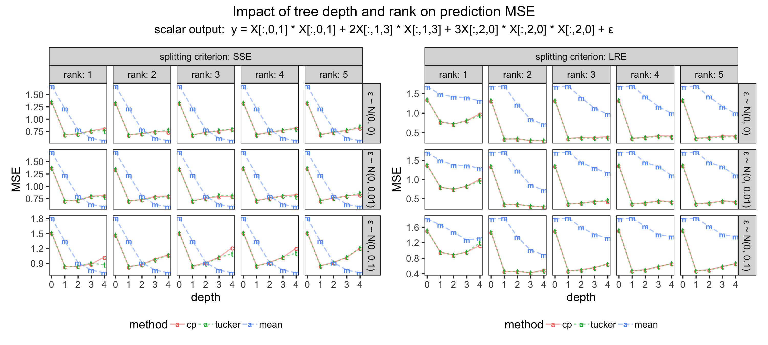
Figure 5: Out-of-sample MSE comparison of CP, Tucker (which both depend on the chosen ranks with $\tau=1$), and mean predictions (which do not depend on the ranks) for tree models of different maximal depths and split by either the SSE (12) or LRE (14) criterion. The data uses a $(1000,5,4)$ input tensor sampled uniformly randomly from $[-1,1]$. The figure shows MSEs averaged over 10 seeds.

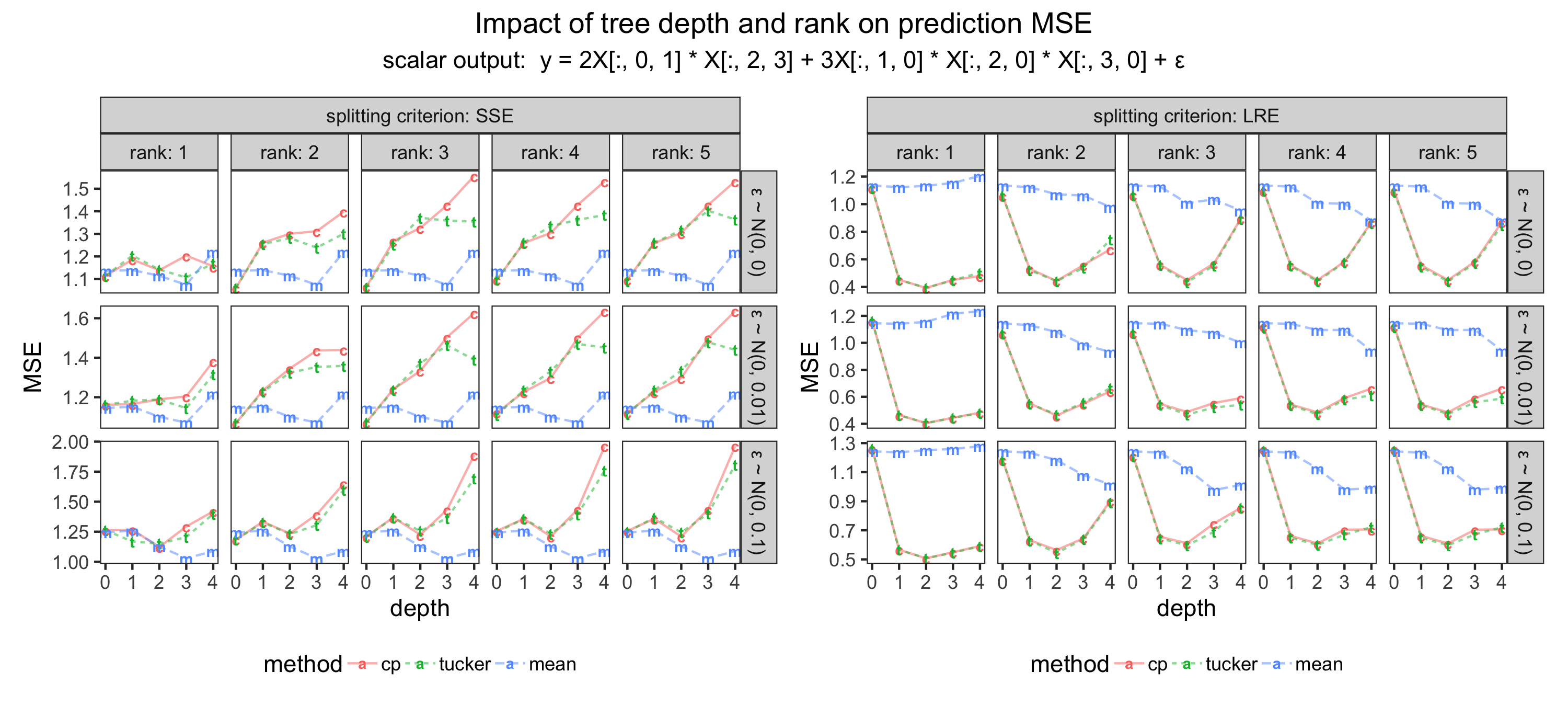
Figure 6: Out-of-sample MSE comparison of CP, Tucker (which both depend on the chosen ranks with $\tau=1$) and mean predictions (which do not depend on the ranks) for tree models of different maximal depths and split by either the SSE (12) or LRE (14) criterion. The data uses a $(1000,5,4)$ input tensor sampled uniformly randomly from $[-1,1]$. The figure shows MSEs averaged over 10 seeds. *In the SSE experiment with rank 2 and $N(0,0.1)$ noise, we found 4 out of 10 cases raising possible non-convergence warnings from $\mathtt{tensorly}$, for other experiments there are 1 or 2.

Splitting criteria allow tree-based regression models to capture interactions between the predictors that would not be captured by a standard regression model (Ritschard, 2013). This approach can also be generalized to tensors of any order. Conditioned on the splitted partitions, we may take the sample mean as predictive values, or fit a regression model (e.g., linear or tensor regression) to the data on each partition.

The standard setting of our model is to let the split_rank parameter to be the same as CP_reg_rank (or Tucker_reg_rank, see Table 5 for detailed parameter specification). In most of the applications considered in this paper, we set split_rank to be the same as the rank chosen for the leaf node regressions. This practice reflects our belief that the model and recursive partition regime share the same low-rank structure assumption. However, it is possible to choose split and regression ranks to be different. The rationale is that when we use one low-rank structure to partition the observations, the low-rank structure within each group might change and hence need a different low-rank assumption. More generally, we can adaptively choose a different target split_rank when we split each layer of the tree using the LAE criterion (13). A common choice is to shrink the target rank as the tree grows deeper, since we have fewer data per split.

Selecting splitting criteria. We examine the MSE in Figures 5 and 6. When split using the SSE criterion (4), the tensor models appear to perform comparably with the mean model, with neither consistently outperforming the other. The underlying mechanisms that split the data according to the variation of $\bm{y}$ do not necessarily capture the tensor structure better.

In contrast, when split using the LRE criterion (14), the tensor models perform better than the mean models. Hence the remainder of the subsection highlights the enhanced performance of tensor models when utilizing the LRE criterion. Interestingly, the MSE of the CP/Tucker models does not monotonically decrease as decomposition rank and tree depth increase. In Figures 5 and 6, the MSEs at rank 1 are different from the MSEs at ranks 2,3,4,5. Rank also seems to affect MSEs at larger tree depths. Otherwise, rank seems to not make much difference in these two examples. Regarding depth, Figure 5 shows that with an appropriate rank (i.e., ranks 2,3,4,5), our tree-based low-rank model exhibit an L-shaped MSE pattern with respect to depth can outperform the mean model for any of the tested tree depths. However, in Figure 6, the CP/Tucker models exhibit a U-shaped MSE pattern with respect to depth and may perform worse than a mean model if the tree depth is not appropriately selected. Specifically, plain CP/Tucker low-rank regression (depth 0) is shown to perform the same as mean regression, but combining low-rank regression with tree structure drastically improves the prediction results (as also shown in Figure 5).

Interaction in signals. The tensor model is quite good at capturing the non-separable interactions like $\bm{X}[:,1,3]*\bm{X}[:,1,3]$ and $\bm{X}[:,1,0]*\bm{X}[:,2,0]*\bm{X}[:,3,0]$ in the tensor input. In Figures 5 and 6, where triplet interactions $\bm{X}[:,2,0]*\bm{X}[:,2,0]*\bm{X}[:,2,0]$ or $\bm{X}[:,1,0]*\bm{X}[:,2,0]*\bm{X}[:,3,0]$ exist, the 3-way tensor decomposition helps to fit a low-rank regression model to outperform the usual mean model used along with tree regressions.

On one hand, increasing the regression ranks will have a saturation effect, where the performance may not change after a certain rank threshold. This is clear in both LAE and LRE columns. The difference is that increasing LAE may deteriorate the performance (Figure 5) while LRE cannot deteriorate the performance, since it is purely splitting based on reducing the tensor regression ranks of the chosen leaf models.

On the other hand, the tree depth (max_depth) will not have this saturation effect. We can observe that there is usually a ’sweetspot’ depth (e.g., depth 1, 2,3 in Figure 6). If we keep increasing the tree depth, we will enter the second half of the U-shape and deteriorate the tree-based tensor-model.

As shown by Figures 5 and 6, the low-rank CP regression models at leaf nodes significantly improve prediction MSE compared to the traditional mean predictions. The performance of low-rank Tucker regression models at leaf nodes, however, depends on the choice of ranks and the depth of the tree.

5.2 Comparison with Other Tensor Models

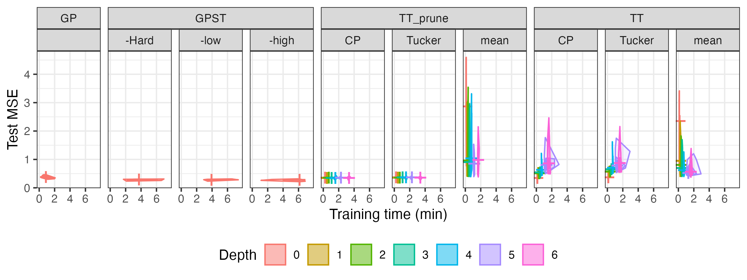
Figure 7: Bagplots (i.e., 2-d generalization of boxplots, Marwick (2024)) for an out-of-sample MSE (mean squared error) comparison between our tensor-input tree (TT), tensor-GP (Yu et al., 2018), GPST (Sun et al., 2023) and CP (ranks = 3), Tucker (ranks = [3,3,3]). All models are fitted (with 75% training set of size 1000 4-dimensional tensor) on 20 batches of the synthetic datasets in Table 1 of Sun et al. (2023). Our TT model is split using SSE criterion (12). For the TT_prune methods, the maximum depth is displayed but the tree is pruned with $\alpha=0.1$ in (22).

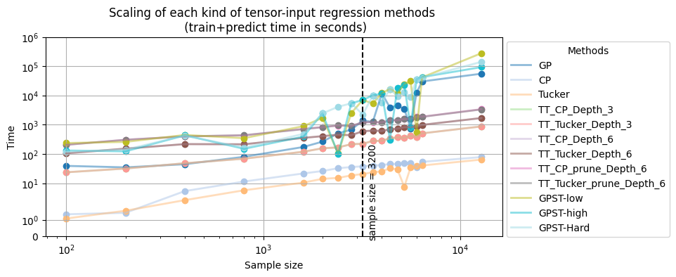
Figure 8: The in-sample and out-of-sample training time (seconds) scaling plot against the sample size for the experiments in Figure 7. For TT models with pruning, we select $\alpha=0.5$ in (22) and perform only one fit on an Intel i9-10885H 2.40GHz machine. TT models with max_depth = 3 or smaller always take less time to produce a comparable fit to tensor-GP (Yu et al., 2018), but when the sample size is greater than 3200, TT methods scales linearly while all GP-based methods (GP, GPST-*) hits the scaling bottleneck.

The Tensor Gaussian Process (TensorGP, Yu et al. (2018)) extends Gaussian Processes (GPs, Luo et al. (2022)) to high-dimensional tensor data using a multi-linear kernel with a low-rank approximation. In regular GPs, the covariance matrix $\bm{K}$ is derived from a kernel function $k(\bm{X},\bm{X}^{\prime})$ which typically depends on the Euclidean distance between points $\bm{X},\bm{X}^{\prime}$. For $n$ data points, the matrix $\bm{K}$ has size $n\times n$ with elements $\bm{K}_{ij}=k(\bm{X}[i,:],\bm{X}[j,:])$.

In TensorGP, the kernel is constructed using a low-rank Tucker tensor decomposition approach. Given tensor data with dimensions corresponding to different features, TensorGP constructs Tucker components (8) like matrices $\mathbf{A}_{1},\mathbf{A}_{2},\mathbf{A}_{3}$ for each dimension. These matrices provide a compact representation of the data in each respective dimension. The covariance matrix $\bm{K}$ is then approximated using the Kronecker product of these matrices, i.e., $\bm{K}\approx\bm{U}\otimes\bm{U}^{\top}+\sigma^{2}\bm{I}$ where $\bm{U}$ is the low-rank approximant $\mathbf{A}_{1}\times_{2}\mathbf{A}_{2}\times_{3}\mathbf{A}_{3}$ and $\sigma^{2}$ is the nugget variance. In our case where we treat the first dimension of the tensor as the number of samples, we will treat the other dimensions as features.

This approach significantly reduces the computational complexity from the $\mathcal{O}(n^{3})$ complexity by GP to a more manageable level, especially for high-dimensional data. The optimization of the TensorGP model involves finding the best low-rank matrices that capture the underlying structure of the data. By doing so, TensorGP maintains the core principles of GP modeling—using a covariance kernel to capture relationships between data points—in a tensor format. Analogous to projection-pursuit (Barnett et al., 2014; Hawke et al., 2023), the Tensor-GPST model (Sun et al., 2023) integrates tensor contraction with a Tensor-GP for dimensionality reduction, employing tensor mode products. This approach is analogous to applying a PCA for dimension reduction before fitting regular GP, where anisotropic total variation regularization is introduced during tensor contraction, creating sparse, smooth latent tensors.

Figure 7 uses the synthetic data from Sun et al. (2023) to compare each model’s performance on training and testing datasets. GPST (low/high/Hard) attains the best testing MSE followed by (tensor-)GP, which shows their exceptional fitting and generalization ability. On the other hand, our tensor tree models obtain lower training MSE (not shown) but much higher testing MSE, which suggests that TT is overfitting the training data and hence might benefit from pruning using our proposed complexity measure (22). Interestingly, in terms of testing MSE, such pruning impairs TT with mean leaf models but also greatly improves TT with CP/Tucker leaf models which are now comparable to GP but still worse than GPST. We find that for any maximum depth setting, the pruned tree models using CP/Tucker leaf models are pruned back to depth 0 whereas the mean models tend to be pruned back to depth 1. However, Figures 7 and 8 also show that GPST has by far the longest training and prediction times, and that our TT models without pruning have the best fitting and predicting times. With pruning, our TT models take longer to compute, but all TT models with depth $\leq 3$ take still much less time to compute than the tensor GP models, echoing our Proposition 3.

5.3 More Applications

EEG Data

Our first example uses the EEG dataset from Li and Zhang (2017) in the $\mathtt{TRES}$ R package. We use $61\times 64\times 64$ tensor inputs of $n=61,d_{1}=d_{2}=64$ parsed from EEG dataset and a binary response $\bm{y}$.

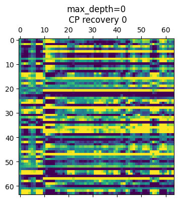
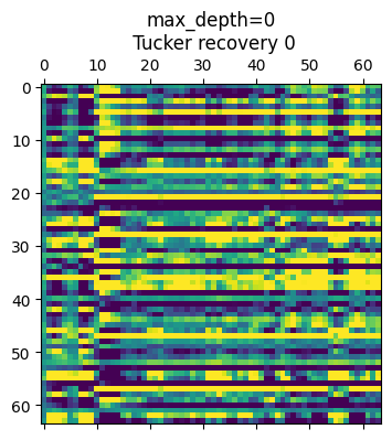
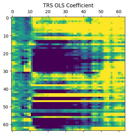
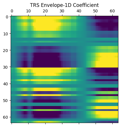
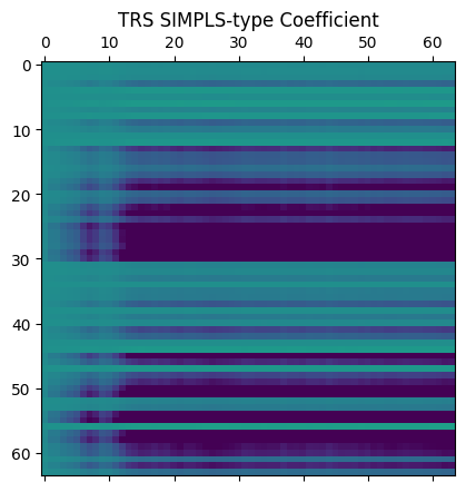
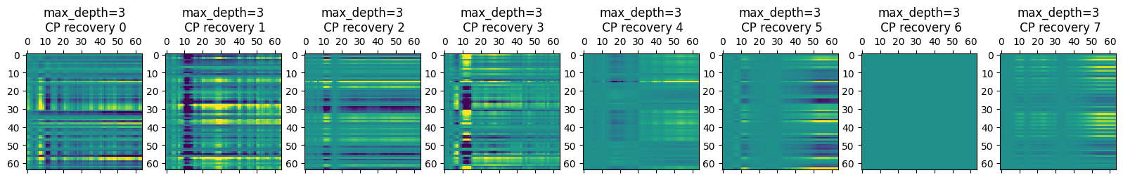
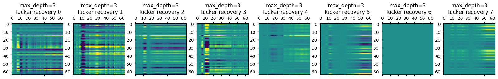
Figure 9: The tensor-input decision tree regression coefficients on an EEG dataset in Li and Zhang (2017). The first row is the coefficients from CP ($R=5$), Tucker ($R=5$), TRS-OLS, TRS-1D and TRS-PLS tensor input models. The second row is coefficients from tensor input tree regression model with depth 3 and leaf node CP models $m_{j}$ ($R=5$). The third row is coefficients from tensor input tree regression model with depth 3 and leaf node Tucker models $m_{j}$ ($R=5$).

Analogous to Figure 1, the second and third rows in Figure 9 consist of eight panels, each of which represents coefficients based on subsets (induced by low-rank splitted trees with target rank $R=5$) along the first dimension of the tensor $\bm{X}$. Each panel visualizes coefficients corresponding to a low-rank CP or Tucker model at leaf nodes, which are based on a subset along the first mode.

We first compare the typical CP and Tucker regression model coefficients (in panels 1,2 of the first row) against the coefficients of tensor input trees (in the second and third rows). The eight panels in the second and third rows appear to overlap and collectively approximate the first two panels in the first row. This can be attributed to several factors. One is the redundancy in the subsets along the first dimension; if these subsets either overlap significantly or are highly correlated, the resulting reconstructions in each panel would naturally appear similar, otherwise dis-similar. Another explanation could be the complementarity of the features captured in each panel. If each panel captures unique but complementary structural or informational elements of the original tensor, their collective representation would naturally approximate the entire tensor effectively. Lastly, the inherent nature of CP and Tucker decomposition as a low-rank approximation implies that even a subset of the first dimension’s factor vectors, when integrated with the corresponding vectors from other modes, can capture significant global features of the original tensor $\bm{X}$.

We then compare the TRS regression model (Li and Zhang, 2017) coefficients (in panels 3,4,5 of the first row) against the coefficients of tensor input trees (in the second and third rows). We can still observe the overlapping phenomena, but different patterns shown in tensor input tree model seems to align with the TRS coefficient patterns well. In particular, the 3,4,5-th leaf node models’ coefficients capture the TRS (OLS, 1D) coefficient patterns.

Facial Image

Our second example uses frontalized facial images as in Lock (2018) showing forward-facing faces achieved by rotating, scaling, and cropping original images. The highly aligned images facilitate appearance comparisons. Each image has $90\times 90$ pixels, with each pixel containing red, green, and blue channel intensities, resulting in a $90\times 90\times 3$ tensor per image. We randomly sample 500 images, so the predictor tensor $\bm{X}$ has dimensions $500\times 90\times 90\times 3$, and the response tensor $\bm{Y}$ has dimensions $500\times 72$. We center each image tensor by subtracting the mean of all image tensors. Another randomly sampled 500 images and response are used as a validation set.

Although Lock (2018) reported that their rrr method with a regularization term $\lambda=10^{5}$ yielded the best prediction result as reported in the original paper of RPE 0.568 and a range from 0.5 to 0.9, it is difficult to fairly compare non-zero regularizations. At each leaf $t$, we can add a regularization term $\lambda(t)$ to the loss function used for the leaf node model, either CP or Tucker. It is unlikely that each leaf model will have the best prediction performance with a shared regularization term $\lambda(t)=\lambda_{TT}$, since the leaf nodes will likely have different sample sizes. Because it is not clear how to adaptively choose this regularization term for leaf models, we choose to enforce all models to have no regularization term (i.e., $\lambda_{TT}=0$). Table 4 shows that TTentrywise and TTlowrank both perform reasonably (although not as good as rrr method) compared to the tensor-on-tensor rrr and its Bayesian rrrBayes models (Lock, 2018). TT provides an alternative adaptive non-parametric modeling for tensor-on-tensor regression without refined prior specification, MCMC computations, or sampling plans (Gahrooei et al., 2021; Luo and Zhang, 2022; Wang and Xu, 2024). However, fitting such a high-dimensional input remains quite challenging for TT models due to the need to compute SSE and LRE in order to split and prune; the output space for TTentrywise requires $72\times 10\text{(number of estimators in ensemble)}=720$ different tree models of depth 3, each of which needs splitting and pruning. Even with the techniques we introduced, the computational cost is rather high compared to rrr.

	TTentrywise_CP		TTentrywise_Tucker		TTlowrank_CP		TTlowrank_Tucker
rank	RMSE	RPE	RMSE	RPE	RMSE	RPE	RMSE	RPE
3	9.0007	0.7083	9.0218	0.7150	8.8316	0.6566	11.7500	2.0573
5	9.0523	0.7247	9.0729	0.7313	8.8761	0.6699	12.072	2.2924
15	9.0582	0.7266	9.1162	0.7454	8.9741	0.7000	10.5614	1.3447

Table 4: The tensor-input decision tree regression coefficients on a resampled Facial Image dataset in Lock (2018). The RMSE and RPE from TT models for tensor-on-tensor regression with CP/Tucker methods and TTentrywise/TTlowrank approaches ($R=3,5,15$) are reported.

6 Conclusion

6.1 Contributions

Our current paper contains contributions to the field of scalar-on-tensor and tensor-on-tensor regressions with a tree-based approach, particularly emphasizing regression tree models for high-dimensional tensor data. A notable innovation is the development of scalar-output regression tree models specifically designed for tensor (multi-way array) inputs. This approach marks a significant departure from traditional regression trees, which typically handle vector inputs, thereby extending the applicability of tree-based models to more complex, multi-dimensional data.

A key strength of our work lies in the development of both randomized and deterministic algorithms tailored for efficiently fitting these tensor-input trees. This advancement is particularly important considering the computational intensity typically associated with tensor operations. Our models demonstrate competitive performance against established tensor-input Gaussian Process models by Sun et al. (2023) and Yu et al. (2018), with the added advantage of reduced computational resource requirements by proposing strategies like leverage score sampling and branch-and-bound optimization to mitigate the computational challenges in tensor operations. This efficiency, coupled with the demonstrated effectiveness, positions these models as a valuable tool in high-dimensional data analysis.

Building on the scalar-on-tensor framework, we extend the methodology to address tensor-on-tensor regression problems using tree ensemble approaches. This and previous works on scaling tree models (Chen and Guestrin, 2016) and Bayesian tree-based models like BART (Luo and Pratola, 2022) show that ensemble tree-based modeling has under-explored potential in building scalable models (See Figure 8). Our extension addresses a notable gap in existing non-parametric supervised models that can handle both tensor inputs and outputs, employing a divide-and-conquer strategy that captures the heterogeneity (Figure 1), allows tensor models at leaf nodes (Algorithm 1) with tensor-input splitting criteria, and may be extended its applicability to wider scenarios like tensor compression (Kielstra et al., 2024). Moreover, we introduce new splitting criteria for trees with tensor inputs, including variance splitting and low-rank approximation.

Theoretically, although we have shown coefficient estimates for fixed trees, the consistency of dynamic trees is not known when the leaf node model is CP or Tucker regression. While the prediction error bound holds for mean leaf node models, it remains unknown whether it holds for CP or Tucker regressions. For ensembles, although we empirically showed the superiority of the gradient boost and random forest ensembles of tensor trees, their consistency and error bounds remains to be derived.

Our paper makes contributions to tree-based non-parametric regression models in the context of tensor data. By addressing computational efficiency (Algorithm 3 and 4), extending our methodologies to tensor-on-tensor problems with ensembling techniques, and introducing new splitting criteria, this work expands the applicability of tree-based models in handling complex, high-dimensional data sets. Building upon the current advancements in tensor-on-tensor regression, future research could explore several intriguing avenues within a concise scope. This expansion promises to enhance the model’s ability to capture complex data interactions.

6.2 Future Works

There are other types of tensor products, such as the Khatri-Rao products, which offer granular feature spaces and detailed splitting rules (Section 2.1). Additionally, kernel-based approaches are well-suited for capturing complex, non-linear relationships and could enhance the predictive power for mixed inputs (Luo et al., 2024). In this direction, practitioners could also explore clustering algorithms on tensor product structures to create sophisticated partitions of the input space (Krawczyk, 2021). A more general form of split rules can be written as $\bm{X}\odot\bm{v}>c$ or $\mathcal{K}(\bm{X},\bm{v})>c$ (analogous to oblique trees Breiman et al. (1984)), where $\odot$ is Khatri-Rao product and $\mathcal{K}$ is a kernelized partition function. Such partition boundaries may not align with the coordinate axes but the splitting on predictive locations may need to be determined by training a classifier based on the clustering algorithm (Luo et al., ress).

Selecting the rank for splitting criteria and leaf tensor models remains an open problem. A optimization-based method or adaptive rank selection via tree models, performed dynamically in a layer-wise manner, could be more flexible than Bayesian shrinkage (Johndrow et al., 2017). Adaptive TT methods could benefit from dynamic rank strategies, such as different target ranks for different layers or incorporating a GCV-term for the target rank into the complexity measure (Section 2.3). This would allow both ranks in splitting criteria and leaf model ranks to be chosen adaptively during tree pruning, which might improve performance, and reveal possible trade-off between shrinkage prior (Wang and Xu, 2024; Lock, 2018) and regularization via pruning.

Another promising direction for future research is to incorporate cross-validation between sub-models in an ensemble, particularly for models using LAE and LRE criteria in ensemble methods, as discussed in Section 3. This approach can reduce the ensemble and diversify sub-models, and aligns with the idea by Blockeel and Struyf (2002), where cross-validation enhances the performance of tree-based models through more refined error evaluation and model selection.

The oracle bounds when using LRE and LAE along with TT models remains open, and developing a robust theoretical framework for these algorithms would enhance our understanding of their behavior and provide guidelines for their practical applications.

Bayesian and additive variants of the TT model and its BART analog with appropriate prior specifications is a very interesting and imminent direction for future work. Additionally, integrating soft decision tree methodologies, such as softBART (Linero and Yang, 2018), tensor Gaussian Processes (Yu et al., 2018) could offer a hybrid approach that combines interpretability with robust uncertainty quantification inherited from Bayesian framework (Shi and Shen, 2023). Such hybrid models could leverage the strengths of both Bayesian and frequentist approaches, providing more flexible and reliable predictive models.

Appendices

Appendix A Algorithms for Fitting Tensor Trees

 

Result: Train a vector input single decision tree regressor and predict with it

Function fit($\bm{X}\in\mathbb{R}^{n\times d}$, $y\in\mathbb{R}^{n}$): begin

       Initialize root node

      for node in tree do

             Calculate for all potential splits along each column $j_{1}\in\{1,2,...,d\}$: Find $\arg\min_{j_{0}\in\{1,\cdots,n\},j_{1}\in\{1,\cdots,d\}}SSE(j_{0},j_{1})$;

             With the minimizer $(j_{0}^{*},j_{1}^{*})$ we split the dataset on the chosen column $j_{1}^{*}$ and splitting value $\bm{X}[j_{0}^{*},j_{1}^{*}]$, creating left and right child nodes using data in $R_{1},R_{2}$;

            

       end for

      Fit the chosen mean/CP/Tucker models at each of the leaf nodes.

end

 

Algorithm 2 Fitting vector input decision tree regressor with SSE criterion (3).

 

Result: Train a tensor input single decision tree regressor with leverage score sampling

Function fit($\bm{X}\in\mathbb{R}^{n\times d_{1}\times d_{2}}$, $\bm{y}\in\mathbb{R}^{n}$):

begin

       Initialize root node and sample_rate $\tau\in(0,1]$ (when $\tau=1$ there is no subsampling). Compute the variance matrix $\bm{V}=\left(\bm{X}[:,i,j]\right)_{i,j=1}^{d_{1},d_{2}}$;

       for node in tree do

             Take a random subset $D\subset\{1,2,...,d_{1}\}\times\{1,2,...,d_{2}\}$ of cardinality $\tau d_{1}d_{2}$ such that the probability of selecting dimension pair $(j_{1},j_{2})$ is proportional to $\bm{V}_{j_{1},j_{2}}$;

             Calculate for all potential splits along each dimension pair $(j_{1},j_{2})\in D$: Find $\arg\min_{j_{0}\in\{1,\cdots,n\},(j_{1},j_{2})\in D}LAE(j_{0},j_{1},j_{2})$ or $LRE(j_{0},j_{1},j_{2})$;

             With the minimizer $(j_{0}^{*},j_{1}^{*},j_{2}^{*})$ we split the dataset on the chosen dimension pair $(j_{1}^{*},j_{2}^{*})$ and splitting value $\bm{X}[j_{0}^{*},j_{1}^{*},j_{2}^{*}]$, creating left and right child nodes using data in $R_{1},R_{2}$;

            

       end for

      Fit the chosen mean/CP/Tucker models at each of the leaf nodes.

end

 

Algorithm 3 Method 1: Leverage score sampling for fitting tensor input decision tree regressor with low-rank splitting criteria (13) and (14).

 

Result: Train a tensor input single decision tree regressor with branch-and-bound optimization

Function fit($\bm{X}\in\mathbb{R}^{n\times d_{1}\times d_{2}}$, $\bm{y}\in\mathbb{R}^{n}$):

begin

       Initialize root node;

       for node in tree do

             Take the full set $D=\{1,2,...,d_{1}\}\times\{1,2,...,d_{2}\}$ of cardinality $d_{1}d_{2}$;

             Calculate for all potential splits along each dimension pair $(j_{1},j_{2})\in D$: Use $best\_idx$ as $(j_{1},j_{2})$ from the return of BnB_minimize($LAE$,$D$,$\xi$) or BnB_minimize($LRE$,$D$,$\xi$);

             With the minimizer $(j_{0}^{*},j_{1}^{*},j_{2}^{*})$ we split the dataset on the chosen dimension pair $(j_{1}^{*},j_{2}^{*})$ and splitting value $\bm{X}[j_{0}^{*},j_{1}^{*},j_{2}^{*}]$, creating left and right child nodes using data in $R_{1},R_{2}$;

            

       end for

      Fit the chosen mean/CP/Tucker models at each of the leaf nodes.

end

Function BnB_minimize($obj$,$D$,$\xi$):

begin

       Set $best\_obj$ to infinity; Set initial bounds $D$ for tensor dimensions and append $D$ to queue;

      

      while queue is not empty do

             $D_{c}$ = queue.pop(0);

            

            mid_feature_index = tuple((b[0] + b[1]) // 2 for b in current $D_{c}$);

            Calculate $obj$ at mid_feature_index;

             if $obj<best\_obj$ then Update $best\_obj$, $best\_idx$;

             for i in range(len($D_{c}$)) do

                   if $D_{c}$[i][1] - $D_{c}$[i][0] > tolerance $\xi$ then

                         mid_point = ($D_{c}$[i][0] + $D_{c}$[i][1]) // 2;

                         left_bounds = right_bounds = $D_{c}$;

                         left_bounds[i] = ($D_{c}$[i][0], mid_point);

                         right_bounds[i] = (mid_point + 1, current_bounds[i][1]);

                         queue.append(left_bounds,right_bounds);

                         break;

                        

                   end if

                  

             end for

            

       end while

      Return $best\_obj$, $best\_idx$ ;

      

end

 

Algorithm 4 Method 2: Branch-and-bound optimization for fitting tensor input decision tree regressor with low-rank splitting criteria (13) and (14).

Appendix B Proof of Proposition 3

Proof.

Since each decomposition when constructing the tree structure takes no more than $N^{*}<\infty$ iterations, it suffices to consider per iteration complexity as stated in Lemmas 1 and 2.

(1) The computational complexity at any node $t$ with $n_{t}$ samples is $\mathcal{O}(n_{t}d_{1}d_{2})$ for finding the best split. In a balanced binary tree with $n$ samples in $\mathbb{R}^{d_{1}\times d_{2}}$, $i$-th level has $2^{i}$ nodes, each processing $\mathcal{O}(n2^{-i})$ samples. The complexity per node is then $\mathcal{O}\left(n2^{-i}\cdot d_{1}d_{2}\right)$. Hence, the total complexity for level $i$ is $2^{i}\cdot\mathcal{O}\left(n2^{-i}\cdot d_{1}d_{2}\right)=\mathcal{O}(nd_{1}d_{2})$. Summing over all $K$ levels, the overall complexity is $\mathcal{O}(n\cdot d_{1}d_{2}\cdot\log k)$.

(2) Now the total complexity for level $i$ is $2^{i}\cdot\mathcal{O}\left(d_{1}d_{2}n2^{-i}\right)\cdot\mathcal{O}\left(d_{1}d_{2}n2^{-i}\right)$. The first factor $\left(d_{1}d_{2}n2^{-i}\right)$ comes from the search of all samples at each coordinate combination in each node at this level. The second factor $\left(d_{1}d_{2}n2^{-i}\right)$ comes from setting $R=n2^{-i}$ and $K=2$ in Lemma 1 since the maximum rank of tensor decomposition cannot exceed the number of sample sizes. Summing over all $\log k$ levels, the overall complexity is $\mathcal{O}(n^{2}d_{1}^{2}d_{2}^{2}\cdot\log k)$.

(3) Now the total complexity for level $i$ is

$$2^{i}\cdot\mathcal{O}\left(d_{1}d_{2}n2^{-i}\right)\cdot\mathcal{O}\left(n2^{-i}d_{1}d_{2}\cdot\min(d_{1}d_{2},n2^{-i})+n2^{-i}d_{1}d_{2}\cdot\min(n2^{-i}d_{1},n2^{-i}d_{2},d_{2},d_{1})\right).$$

The first factor $\left(d_{1}d_{2}n2^{-i}\right)$ comes from the search of all samples at each coordinate combination in each node at this level. The second factor come from setting $R=n2^{-i}$ and $K=2$ in Lemma 2. Summing over all $\log k$ levels, the overall complexity is $\mathcal{O}\left(\log k\cdot n^{2}d_{1}^{2}d_{2}^{2}\cdot\left(\min(d_{1}d_{2},n)+\min(nd_{1},nd_{2},d_{2},d_{1})\right)\right)$. Then we can simplify the term $\min(nd_{1},nd_{2},d_{2},d_{1})$ to $\min(d_{2},d_{1})$ since we know that $n\geq 1$ by assumption. ∎

Appendix C Proof of Lemma 2

Proof.

The argument is as follows, since the complexity bottleneck per iteration comes from the SVD step:

$$\mathcal{O}\left(\min\left\{n\prod_{j=1}^{K}d_{j}^{{}^{\prime}2},n^{2}\prod_{j=1}^{K}d_{j}^{{}^{\prime}}\right\}+\sum_{i=1}^{K}\min\left\{R^{2}\cdot d_{i}\prod_{j\neq i}d_{j}^{{}^{\prime}2},R\cdot d_{i}^{2}\prod_{j\neq i}d_{j}^{{}^{\prime}}\right\}\right)$$

$$\asymp \mathcal{O}\left(\min\left\{n\prod_{j=1}^{K}d_{j}^{{}^{\prime}2},n^{2}\prod_{j=1}^{K}d_{j}^{{}^{\prime}}\right\}+\sum_{i=1}^{K}\min\left\{R^{2}\cdot\frac{d_{i}}{d_{i}^{{}^{\prime}2}}\prod_{j=1}^{K}d_{j}^{{}^{\prime}2},R\cdot\frac{d_{i}^{2}}{d_{i}^{{}^{\prime}}}\prod_{j=1}^{K}d_{j}^{{}^{\prime}}\right\}\right)$$

$$\asymp \mathcal{O}\left(\min\left\{n\prod_{j=1}^{K}d_{j}^{2},n^{2}\prod_{j=1}^{K}d_{j}\right\}+\sum_{i=1}^{K}\min\left\{R^{2}\cdot\frac{1}{d_{i}}\prod_{j=1}^{K}d_{j}^{2},R\cdot d_{i}\prod_{j=1}^{K}d_{j}\right\}\right)\text{ since }d_{i}^{{}^{\prime}}\asymp d_{i},$$

$$\lesssim \mathcal{O}\left(n\prod_{j=1}^{K}d_{j}^{2}+\sum_{i=1}^{K}R\cdot d_{i}\prod_{j=1}^{K}d_{j}\right)$$

Because $R<n$, in the preceding line the first summand dominates the second summand. We conclude the proof by noting that $\prod_{i=1}^{K}d_{i}^{2}\leq(\max_{i}d_{i})^{2K}$. ∎

Appendix D Proof of Theorem 5

Proof.

The proof is almost identical to the proof of Theorem 4.2 in Klusowski and Tian (2024) since when minimizing (12) and splitting at each interior node we indeed “flatten” the input tensor $\bm{X}$ along its second and third coordinates. We consider the maximum impurity gain $IG(t)$ for $N_{t}$ samples in node $t$ to decrease the empirical risk for the regressor $g$

$$\hat{\mathcal{R}}_{t}(g)=\frac{1}{N_{t}}\sum_{\bm{X}^{(n)}[i,:,:]\in t}\mathcal{L}(y_{i},g(\bm{X}^{(n)}[i,:,:]))$$ ,

for the chosen loss function $\mathcal{L}$ (e.g., (3) and (4)) in the parent node $t$. When we split node $t$ into left and right nodes

$$t_{L} \coloneqq\left\{\bm{X}\in t\colon\bm{X}[:,j_{1},j_{2}]\leq s\right\},N_{t_{L}}=\#\{\bm{X}^{(n)}[i,:,:]\in t_{L}\},$$

$$t_{R} \coloneqq\left\{\bm{X}\in t\colon\bm{X}[:,j_{1},j_{2}]>s\right\},N_{t_{R}}=\#\{\bm{X}^{(n)}[i,:,:]\in t_{R}\}$$

we have an analog to Lemma A.1 in Klusowski and Tian (2024) for the $\ell_{2}$ inner product between multivariate functions $u$ and $v$. At node $t$, this inner product is evaluated only at those observed locations $\bm{X}^{(n)}[i,:,:]\in t$:

$$\left\langle u,v\right\rangle_{t} \coloneqq\frac{1}{N_{t}}\cdot\sum_{\bm{X}^{(n)}[i,:,:]\in t}u(\bm{X}^{(n)}[i,:,:])\cdot v(\bm{X}^{(n)}[i,:,:])=\frac{1}{N_{t}}\cdot\sum_{\bm{X}^{(n)}[i,:,:]\in t}\sum_{j,k}u(\bm{X}[i,j,k])\cdot v(\bm{X}[i,j,k])\text{ for \eqref{eq:sse-tensor}}.$$

The key idea in proving the impurity gain lower bound is to use a linear interpolator over the domain $\mathbb{R}$ indexed by $\mathbb{N}\times\mathbb{N}$, for the ordered statistics $\bm{X}[(1),j_{1},j_{2}]\leq\cdots\leq\bm{X}[(n),j_{1},j_{2}]$, to control the empirical risk. To attain this goal, we define the probability measure $\Pi(j_{1},j_{2},s)$ for splitting point $s$ and variables $\bm{X}[:,j_{1},j_{2}]$ where its RN derivative with respect to the counting measure on $\mathbb{N}\times\mathbb{N}$ and the Lebesgue measure on $\mathbb{R}$ (this is still defined on $\mathbb{R}$ not $\mathbb{R}^{d_{1}\times d_{2}}$ since the split still happens by one threshold $s$) can be written as

$$\frac{d\Pi(j_{1},j_{2},s)}{d(j_{1},j_{2})\times ds}\coloneqq\frac{\left|Dg_{j_{1},j_{2}}(s)\right|\sqrt{N_{t_{L}}N_{t_{R}}/N_{t}^{2}}}{\sum_{i_{1}=1}^{d_{1}}\sum_{i_{2}=1}^{d_{2}}\int_{\mathbb{R}}\left|Dg_{i_{1},i_{2}}(s^{\prime})\right|ds^{\prime}}$$

$$Dg_{j_{1},j_{2}}(s) = \begin{cases}\frac{g_{j_{1},j_{2}}\left(\bm{X}[(i+1),j_{1},j_{2}]\right)-g_{j_{1},j_{2}}\left(\bm{X}[(i),j_{1},j_{2}]\right)}{\bm{X}[(i+1),j_{1},j_{2}]-\bm{X}[(i),j_{1},j_{2}]}&\bm{X}[(i),j_{1},j_{2}]<s<\bm{X}[(i+1),j_{1},j_{2}]\\ 0&\text{otherwise}\end{cases}.$$

Using these bi-indexed linear interpolators $Dg_{j_{1},j_{2}}(s)$ as piece-wise density functions, we obtain an impurity gain formula for a tensor-input tree when splitting with the SSE criterion and fitting with mean leaf models.

Analog of Lemma 4.1 (Tensor Input Case): Let $g\in\mathcal{G}_{1}$ and $K\geq 1$ be any depth. For any terminal node $t$ of the tree $T_{K-1}$ such that $\hat{\mathcal{R}}_{t}(g_{T_{K-1}})>\hat{\mathcal{R}}_{t}(g)$, we have

$$IG(t)\geq\frac{\left(\hat{\mathcal{R}}_{t}(\hat{g}_{T_{K-1}})-\hat{\mathcal{R}}_{t}(g)\right)^{2}}{V^{2}(g)}$$

where $V(g)=\|g\|_{TV}$ is a complexity constant dependent on $g$.

Next, we proceed with the proof of Theorem 5, which is an analog of Theorem 4.2 of Klusowski and Tian (2024). Since the output is still scalar, we use recursion for empirical risk reduction and get the total risk

$$\hat{\mathcal{R}}(g_{T_{K}})=\hat{\mathcal{R}}(g_{T_{K-1}})-\sum_{t\in T_{K-1}}\frac{N_{t}}{N}IG(t)$$

where $t\in T_{K-1}$ means that $t$ is a terminal node of tree $T_{K-1}$. By the above tensor analog of Lemma 4.1, the total impurity gain over all terminal nodes $t\in T_{K-1}$ such that $\hat{\mathcal{R}}_{t}(g_{T_{K-1}})>\hat{\mathcal{R}}_{t}(g)$ is bounded by

$$\sum_{t\in T_{K-1}\colon\hat{\mathcal{R}}_{t}(g_{T_{K-1}})>\hat{\mathcal{R}}_{t}(g)}\frac{N_{t}}{N}IG(t)\geq\sum_{t\in T_{K-1}\colon\hat{\mathcal{R}}_{t}(g_{T_{K-1}})>\hat{\mathcal{R}}_{t}(g)}\frac{N_{t}}{N}\frac{\left(\hat{\mathcal{R}}_{t}(\hat{g}_{T_{K-1}})-\hat{\mathcal{R}}_{t}(g)\right)^{2}}{V^{2}(g)}.$$

Applying Jensen’s inequality to the sum, we get

$$\sum_{t\in T_{K-1}\colon\hat{\mathcal{R}}_{t}(g_{T_{K-1}})>\hat{\mathcal{R}}_{t}(g)}\frac{N_{t}}{N}\left(\hat{\mathcal{R}}_{t}(\hat{g}_{T_{K-1}})-\hat{\mathcal{R}}_{t}(g)\right)^{2} \geq\left(\sum_{t\in T_{K-1}\colon\hat{\mathcal{R}}_{t}(g_{T_{K-1}})>\hat{\mathcal{R}}_{t}(g)}\frac{N_{t}}{N}\left(\hat{\mathcal{R}}_{t}(\hat{g}_{T_{K-1}})-\hat{\mathcal{R}}_{t}(g)\right)\right)^{2}$$

$$\geq\left(\sum_{t\in T_{K-1}}\frac{N_{t}}{N}\left(\hat{\mathcal{R}}_{t}(\hat{g}_{T_{K-1}})-\hat{\mathcal{R}}_{t}(g)\right)\right)^{2}.$$

The global excess risk can be defined as

$$E_{K}:=\hat{\mathcal{R}}(g_{T_{K}})-\hat{\mathcal{R}}(g).$$

We can rewrite the total impurity gain as

$$\sum_{t\in T_{K-1}}\frac{N_{t}}{N}\left(\hat{\mathcal{R}}_{t}(\hat{g}_{T_{K-1}})-\hat{\mathcal{R}}_{t}(g)\right)=E_{K-1}.$$

Combining the results from steps above, we have

$$E_{K}\leq E_{K-1}\left(1-\frac{E_{K-1}}{V^{2}(g)}\right).$$

By induction, we iterate this inequality to obtain

$$E_{K}\leq\frac{V^{2}(g)}{K+3}.$$

Finally, substituting back into the empirical risk, we obtain

$$\hat{\mathcal{R}}(g_{T_{K}})\leq\hat{\mathcal{R}}(g)+\frac{V^{2}(g)}{K+3}.$$

Taking the infimum over all functions $g$, we get

$$\hat{\mathcal{R}}(g_{T_{K}})\leq\inf_{g\in{\mathcal{G}_{1}}}\left\{\hat{\mathcal{R}}(g)+\frac{V^{2}(g)}{K+3}\right\}.$$

Hence, we have proved an analog of Theorem 4.2 for the tensor input case, where the only difference is the statement and definitions used in the analog of Lemma 4.1. ∎

Appendix E Algorithms for Ensembles of Trees

	variance	clustering	low-rank
Sample average of the $y$	max_depth	max_depth, cluster_method	split_rank, max_depth
CP regression on $y$	max_depth,	max_depth,	split_rank,
	CP_reg_rank	cluster_method,	max_depth,
		CP_reg_rank	CP_reg_rank
Tucker regression on $y$	max_depth,	max_depth,	split_rank,
	Tucker_reg_rank	cluster_method,	max_depth,
		Tucker_reg_rank	Tucker_reg_rank

Table 5: Supported combination methods: TensorDecisionTreeRegressor and associated parameters, and how it generalizes existing models.

 

Result: Forest of decision trees $\{T_{t}\}$

Input: Tensor data $\bm{X}\in\mathbb{R}^{n\times p_{1}\times p_{2}\times\ldots\times p_{d}}$, Target values $y\in\mathbb{R}^{n}$, Number of trees $T$;

for $t\leftarrow 1$ to $T$ do

       $(X_{t},y_{t})\leftarrow\text{Bootstrap sample from }(X,y)$;

       $T_{t}\leftarrow\text{Train a decision tree on }(X_{t},y_{t})$ with random subsampling of predictors at root node;

       Store all observations in each leaf of $T_{t}$;

       Fit the chosen mean/CP/Tucker models at each of the leaf nodes of $T_{t}$;

      

end for

$\bm{y}_{i}^{pred}=\sum_{t=1}^{T}F_{t}(\bm{X}^{(n)}[i,:,:])$;

 

Algorithm 5 Random Forest with Tensor Input

 

Result: Train a generalized boosting regressor model and predict with it

Function GeneralizedBoostingRegressor($\bm{X}\in\mathbb{R}^{n\times d_{1}\times d_{2}}$, $\bm{y}\in\mathbb{R}^{n}$, $M$, $\eta$, $p_{resample}$):

begin

       Initialize $F_{0}(x)$ to the mean of $\bm{y}$;

      

      for $m=1$ to $M$ do

             Compute residuals: $r_{im}=y_{i}-F_{m-1}(\bm{X}^{(n)}[i,:,:])$ for all $i$;

            

            if $p_{resample}>0$ then

                   Sample indices according to weights: $\bm{I}_{resample}\sim\text{Sample}(\text{Indices},\text{Weights},\text{Size}=n\times p_{resample})$;

                   $\bm{h}_{m}$ = fit($\bm{X}[\bm{I}_{resample},:,:]$, $r_{im}[\bm{I}_{resample}]$);

                   Update weights: $\text{Weights}=\text{Weights}\times\exp(\left|r_{im}\right|)$;

                   Normalize weights: $\text{Weights}=\text{Weights}/\sum\text{Weights}$;

                  

            else

                  

             end if

            for each sample $i$ do

                   $\bm{y}_{i}^{pred}=F_{m-1}(\bm{X}^{(n)}[i,:,:])+\eta\bm{h}_{m}(\bm{X}^{(n)}[i,:,:])$;

                  

             end for

            Update $F_{m}(x)=F_{m-1}(x)+\eta\bm{h}_{m}(x)$;

            

       end for

      return $F_{M}(x)$;

      

end

 

Algorithm 6 Generalized Boosting Regressor with Optional AdaBoost-Like Resampling

References

- Amit and Geman (1997) Amit, Y. and D. Geman (1997). Shape quantization and recognition with randomized trees. Neural computation 9(7), 1545–1588.
- Barnett et al. (2014) Barnett, R. M., J. G. Manchuk, and C. V. Deutsch (2014). Projection pursuit multivariate transform. Mathematical Geosciences 46, 337–359.
- Bi et al. (2021) Bi, X., X. Tang, Y. Yuan, Y. Zhang, and A. Qu (2021). Tensors in statistics. Annual review of statistics and its application 8, 345–368.
- Blockeel and Struyf (2002) Blockeel, H. and J. Struyf (2002). Efficient algorithms for decision tree cross-validation. Journal of Machine Learning Research 3(Dec), 621–650.
- Breiman (1999) Breiman, L. (1999). Prediction games and arcing algorithms. Neural computation 11(7), 1493–1517.
- Breiman (2001) Breiman, L. (2001). Random forests. Machine Learning 45, 5–32.
- Breiman et al. (1984) Breiman, L. et al. (1984). Classification and regression trees.
- Chaudhuri et al. (1994) Chaudhuri, P., M.-C. Huang, W.-Y. Loh, and R. Yao (1994). Piecewise-polynomial regression trees. Statistica Sinica, 143–167.
- Chen and Guestrin (2016) Chen, T. and C. Guestrin (2016). Xgboost: A scalable tree boosting system. In Proceedings of the 22Nd ACM SIGKDD International Conference on Knowledge Discovery and Data Mining, KDD ’16, New York, NY, USA, pp. 785–794. ACM.
- Chickering et al. (2001) Chickering, D. M., C. Meek, and R. Rounthwaite (2001). Efficient determination of dynamic split points in a decision tree. In Proceedings 2001 IEEE international conference on data mining, pp. 91–98. IEEE.
- Chipman et al. (1998) Chipman, H., E. I. George, and R. E. McCulloch (1998). Bayesian cart model search. Journal of the American Statistical Association 93(443), 935–948.
- Chipman et al. (2012) Chipman, H., P. Ranjan, and W. Wang (2012). Sequential design for computer experiments with a flexible Bayesian additive model. Canadian Journal of Statistics 40(4), 663–678.
- Chipman et al. (2010) Chipman, H. A., E. I. George, and R. E. McCulloch (2010). Bart: Bayesian additive regression trees. The Annals of Applied Statistics 4(1), 266–298.
- Denison et al. (1998) Denison, D., A. Smith, and B. Mallick (1998). Bayesian cart model search: Comment. Journal of the American Statistical Association 93(443), 954–957.
- Drucker (1997) Drucker, H. (1997). Improving Regressors using Boosting Techniques. In Proceedings of the Fourteenth International Conference on Machine Learning, ICML ’97, pp. 107–115.
- Freund and Schapire (1997) Freund, Y. and R. E. Schapire (1997). A decision-theoretic generalization of on-line learning and an application to boosting. Journal of computer and system sciences 55, 119–139.
- Friedman et al. (2004) Friedman, J., T. Hastie, S. Rosset, R. Tibshirani, and J. Zhu (2004). Discussion of boosting papers. Annual Statistics 32, 102–107.
- Friedman (2001) Friedman, J. H. (2001). Greedy function approximation: A gradient boosting machine. The Annals of Statistics 19, 1189–1232.
- Gahrooei et al. (2021) Gahrooei, M. R., H. Yan, K. Paynabar, and J. Shi (2021). Multiple tensor-on-tensor regression: An approach for modeling processes with heterogeneous sources of data. Technometrics 63(2), 147–159.
- Geurts et al. (2006) Geurts, P., D. Ernst, and L. Wehenkel (2006). Extremely randomized trees. Machine learning 63, 3–42.
- Gordon and Olshen (1978) Gordon, L. and R. A. Olshen (1978). Asymptotically efficient solutions to the classification problem. The Annals of Statistics, 515–533.
- Guhaniyogi et al. (2017) Guhaniyogi, R., S. Qamar, and D. B. Dunson (2017). Bayesian tensor regression. Journal of Machine Learning Research 18(79), 1–31.
- Hastie et al. (2009) Hastie, T., R. Tibshirani, J. H. Friedman, and J. H. Friedman (2009). The elements of statistical learning: data mining, inference, and prediction, Volume 2. Springer.
- Hawke et al. (2023) Hawke, S., H. Luo, and D. Li (2023). Contrastive Inverse Regression for Dimension Reduction. arXiv:2305.12287, 1–35.
- Johndrow et al. (2017) Johndrow, J. E., A. Bhattacharya, and D. B. Dunson (2017). Tensor decompositions and sparse log-linear models. Annals of statistics 45(1), 1.
- Kielstra et al. (2024) Kielstra, P. M., T. Shi, H. Luo, J. Qian, and Y. Liu (2024+). A linear-complexity tensor butterfly algorithm for compressing high-dimensional oscillatory integral operators. ongoing, 1–39.
- Klusowski and Tian (2024) Klusowski, J. M. and P. M. Tian (2024). Large scale prediction with decision trees. Journal of the American Statistical Association 119(545), 525–537.
- Kolda and Bader (2009) Kolda, T. G. and B. W. Bader (2009). Tensor decompositions and applications. SIAM review 51(3), 455–500.
- Kolda and Sun (2008) Kolda, T. G. and J. Sun (2008). Scalable tensor decompositions for multi-aspect data mining. In 2008 Eighth IEEE international conference on data mining, pp. 363–372. IEEE.
- Kossaifi et al. (2019) Kossaifi, J., Y. Panagakis, A. Anandkumar, and M. Pantic (2019). Tensorly: Tensor learning in python. Journal of Machine Learning Research 20(26), 1–6.
- Krawczyk (2021) Krawczyk, B. (2021). Tensor decision trees for continual learning from drifting data streams. Machine Learning 110(11-12), 3015–3035.
- Lawler and Wood (1966) Lawler, E. L. and D. E. Wood (1966). Branch-and-bound methods: A survey. Operations research 14(4), 699–719.
- Li et al. (2000) Li, K.-C., H.-H. Lue, and C.-H. Chen (2000). Interactive tree-structured regression via principal hessian directions. Journal of the American Statistical Association 95(450), 547–560.
- Li and Zhang (2017) Li, L. and X. Zhang (2017). Parsimonious tensor response regression. Journal of the American Statistical Association 112(519), 1131–1146.
- Li et al. (2018) Li, X., D. Xu, H. Zhou, and L. Li (2018). Tucker tensor regression and neuroimaging analysis. Statistics in Biosciences 10, 520–545.
- Linero and Yang (2018) Linero, A. R. and Y. Yang (2018). Bayesian regression tree ensembles that adapt to smoothness and sparsity. Journal of the Royal Statistical Society: Series B (Statistical Methodology) 80(5), 1087–1110.
- Liu (2017) Liu, Y. (2017). Low-rank tensor regression: Scalability and applications. In 2017 IEEE 7th International Workshop on Computational Advances in Multi-Sensor Adaptive Processing (CAMSAP), pp. 1–5. IEEE.
- Lock (2018) Lock, E. F. (2018). Tensor-on-tensor regression. Journal of Computational and Graphical Statistics 27(3), 638–647.
- Loh (2014) Loh, W.-Y. (2014). Fifty years of classification and regression trees. International Statistical Review 82, 329–348.
- Luo et al. (2024) Luo, H., Y. Cho, J. W. Demmel, X. Li, and Y. Liu (2024). Hybrid Parameter Search and Dynamic Model Selection for Mixed-Variable Bayesian Optimization. Journal of Computational and Graphical Statistics 0(0), 1–14.
- Luo et al. (ress) Luo, H., J. W. Demmel, Y. Cho, X. S. Li, and Y. Liu (In press). Non-smooth Bayesian Optimization in Tuning Problems. International Journal of High Performance Computing Applications, 1–61.
- Luo and Ma (2023) Luo, H. and A. Ma (2023+). Tensor randomized frontal sketching method to large-scale linear systems. In preparation, 1–30.
- Luo et al. (2022) Luo, H., G. Nattino, and M. T. Pratola (2022). Sparse Additive Gaussian Process Regression. Journal of Machine Learning Research 23(61), 1–34.
- Luo and Pratola (2022) Luo, H. and M. T. Pratola (2022). Sharded Bayesian Additive Regression Trees. arXiv:2306.00361, 1–46.
- Luo and Zhang (2022) Luo, Y. and A. R. Zhang (2022). Tensor-on-tensor regression: Riemannian optimization, over-parameterization, statistical-computational gap, and their interplay. arXiv preprint arXiv:2206.08756.
- Malik and Becker (2018) Malik, O. A. and S. Becker (2018). Low-rank tucker decomposition of large tensors using tensorsketch. Advances in neural information processing systems 31.
- Marwick (2024) Marwick, B. (2024). Basic bagplot geom for ggplot2. https://gist.github.com/benmarwick/00772ccea2dd0b0f1745.
- Mentch and Zhou (2020) Mentch, L. and S. Zhou (2020). Randomization as regularization: A degrees of freedom explanation for random forest success. The Journal of Machine Learning Research 21(1), 6918–6953.
- Minster et al. (2023) Minster, R., I. Viviano, X. Liu, and G. Ballard (2023). Cp decomposition for tensors via alternating least squares with qr decomposition. Numerical Linear Algebra with Applications 30(6), e2511.
- Morrison et al. (2016) Morrison, D. R., S. H. Jacobson, J. J. Sauppe, and E. C. Sewell (2016). Branch-and-bound algorithms: A survey of recent advances in searching, branching, and pruning. Discrete Optimization 19, 79–102.
- Murray et al. (2023) Murray, R., J. Demmel, M. W. Mahoney, N. B. Erichson, M. Melnichenko, O. A. Malik, L. Grigori, M. a. M. E. L. Dereziński, T. Liang, H. Luo, and J. J. Dongarra (2023). Randomized numerical linear algebra: A perspective on the field with an eye to software. arXiv preprint arXiv:2302.11474.
- Oh et al. (2018) Oh, S., N. Park, S. Lee, and U. Kang (2018). Scalable tucker factorization for sparse tensors-algorithms and discoveries. In 2018 IEEE 34th International Conference on Data Engineering (ICDE), pp. 1120–1131. IEEE.
- Papadogeorgou et al. (2021) Papadogeorgou, G., Z. Zhang, and D. B. Dunson (2021). Soft tensor regression. Journal of Machine Learning Research 22(219), 1–53.
- Pratola (2016) Pratola, M. T. (2016). Efficient metropolis-hastings proposal mechanisms for bayesian regression tree models. Bayesian Analysis 11, 885–911.
- Pratola et al. (2014) Pratola, M. T., H. A. Chipman, J. R. Gattiker, D. M. Higdon, R. McCulloch, and W. N. Rust (2014). Parallel Bayesian additive regression trees. Journal of Computational and Graphical Statistics 23, 830–852.
- Prokhorenkova et al. (2018) Prokhorenkova, L., G. Gusev, A. Vorobev, A. V. Dorogush, and A. Gulin (2018). Catboost: unbiased boosting with categorical features. Advances in neural information processing systems 31.
- Ritschard (2013) Ritschard, G. (2013). Chaid and earlier supervised tree methods. Contemporary issues in exploratory data mining in the behavioral sciences, 48–74.
- Shi and Shen (2023) Shi, Y. and W. Shen (2023). Bayesian methods in tensor analysis. arXiv preprint arXiv:2302.05978.
- Sun et al. (2023) Sun, H., W. Manchester, M. Jin, Y. Liu, and Y. Chen (2023). Tensor gaussian process with contraction for multi-channel imaging analysis. arXiv preprint arXiv:2301.11203.
- Wang and Xu (2024) Wang, K. and Y. Xu (2024). Bayesian tensor-on-tensor regression with efficient computation. Statistics and its interface 17(2), 199.
- Yu et al. (2018) Yu, R., G. Li, and Y. Liu (2018). Tensor regression meets gaussian processes. In International Conference on Artificial Intelligence and Statistics, pp. 482–490. PMLR.
- Zhou et al. (2013) Zhou, H., L. Li, and H. Zhu (2013). Tensor regression with applications in neuroimaging data analysis. Journal of the American Statistical Association 108(502), 540–552.