Scalable Signal Temporal Logic Guided Reinforcement Learning via Value Function Space Optimization
Abstract
The integration of reinforcement learning (RL) and formal methods has emerged as a promising framework for solving long-horizon planning problems. Conventional approaches typically involve abstraction of the state and action spaces and manually created labeling functions or predicates. However, the efficiency of these approaches deteriorates as the tasks become increasingly complex, which results in exponential growth in the size of labeling functions or predicates. To address these issues, we propose a scalable model-based RL framework, called VFSTL, which schedules pre-trained skills to follow unseen STL specifications without using hand-crafted predicates. Given a set of value functions obtained by goal-conditioned RL, we formulate an optimization problem to maximize the robustness value of Signal Temporal Logic (STL) defined specifications, which is computed using value functions as predicates. To further reduce the computation burden, we abstract the environment state space into the value function space (VFS). Then the optimization problem is solved by Model-Based Reinforcement Learning. Simulation results show that STL with value functions as predicates approximates the ground truth robustness and the planning in VFS directly achieves unseen specifications using data from sensors.
Index Terms:
formal methods, signal temporal logic, reinforcement learning, value function space, planningI INTRODUCTION
As robots are widely deployed in increasingly complicated environments, tasks that span long time horizons become ubiquitous and impose immense challenges. RL enables autonomous agents to acquire complex behaviors through trails and errors, which has been applied in a variety of scenarios ranging from robot navigation to dexterous manipulation, and demonstrated its great potential. However, learning complex long-horizon behaviours remains tough due to the large exploration space and sparsity of rewards, see, e.g.,[22] [27].
To mitigate the issues, formal methods have been incorporated into robot planning and control applications to define structured task specifications [3]. Some recent advances extend Linear Temporal Logic (LTL) to reward engineering [20, 5, 26], multi-task RL[25] and hierarchical RL [2, 10]. For instance, Araki at el. use options to encapsulate sub-policies to satisfy logical formula [2]. These methods are usually based on abstracting states and actions into specifications represented as an automaton, which allows the semantic groundings of LTL properties in the RL framework. This abstraction process is crucial in bridging the gap between low-level RL policies and high-level LTL specifications, ensuring that the execution of actions aligns with the desired temporal properties. However, the size of the discretized state space exponentially increases with its dimensions.
Compared with LTL, Signal Temporal Logic (STL) is more capable to describe a wider range of temporal and real-valued constraints, making it a versatile tool for specifying complex properties in robotics[4]. Despite its strong expressiveness, it is usually computationally expensive to solve STL based planning, learning and control problems, which requires mixed-integer programming[17] or sampling-based[6] approaches. This drawback severely restrains the application of STL to non-linear and high high-dimensional systems, where such methods are impractical. Another mainstream direction is to integrate STL with RL to address safety [14] and long-horizon planning [7, 12] problems, where most relevant works assume that the predicates from signals are given a priori. However, real word signals usually appear as images or point clouds, thus it is more reasonable to build the predicates. Leung at.el. tackled this problem by treating each channel in the input of a convolution neural network as a signal to compute the robustness[9], but their results are only applicable to one particular type of STL formula.
Given the limitations of existing works, we propose a model-based reinforcement learning framework that is capable of satisfying unseen STL specifications by sequencing the execution of pre-learned policies. Our approach leverages the theorem that the value function in goal-conditioned RL represents the probability of achieving the target. We remove the need for hand-crafting predicates by using value function approximations. To solve this planning problem, we then train a multi-layer perceptron to predict the dynamics of value functions. By doing this, we formulate an optimization problem on value function space[19], whose state space is only related to the number of skills, enabling for efficient long horizon planning. This problem is then solved using model-based reinforcement learning approach. We evaluate VFSTL on three randomly generated tasks: sequencing, reach-avoid and stability, where results show that optimizing on value function space approximates the original problem.
The main contributions of this work include: (i) we show that the value function captures the satisfaction probability of a given task in current state in goal-conditioned RL. (ii) we illustrate that the dynamics of the value function space provides ample information about the process of completing the tasks. (iii) We propose a scalable model-based RL framework to achieve planning in the value function space, independent of the low-level system state space dimensions.
The following sections are organized in the following manner. Section II introduces the preliminary knowledge. Section III formally formulates the STL planning problem studied in this work. Section IV proposes the scalable STL guided reinforcement learning framework which approximates the robustness values of STL in the value function space. Then Section V presents the simulation results in an robot planning environment. Finally Section VI concludes the work and includes some potential directions of extension.
II Preliminaries
II-A Signal Temporal Logic
Signal Temporal Logic (STL)[4] is employed to define system behaviors based on real signals , where denotes the discrete time domain. Considering a signal within a specific time frame , where and , STL provides a robustness value that quantifies the degree to which this signal meets a given specification. The interpretation of the results is straightforward: positive values indicate that the STL specification is fulfilled, whereas negative values indicate non-compliance. STL comprises three fundamental elements: predicates , Boolean operators and , and temporal operators constrained by time intervals . It is formally defined in a recursive manner as:
| (1) |
Predicates are functions that convert signals into boolean values, denoted as , typically in the form of , where and is a real number. The ’until’ operator, , holds when remains true up until becomes true. Using existing operators, we can introduce additional temporal concepts. For instance, the ’eventually’ operator is defined as , and the ’globally’ operator is defined as . To express that from a certain time onward, the signal adheres to the STL formula , we use the notation .
The robustness value, , quantifies how well a signal satisfies a STL formula at time . There are several methods to compute this. In our study, we adopt the classic space robustness metric as defined in the referenced work[4]. The robustness value is considered sound when it is positive if and only if . Moreover, the formula encompasses a horizon, , which is calculated recursively based on the bounded temporal operators contained within, as detailed in [4]. Consequently, to evaluate the robustness of the signal starting from time , denoted , it suffices to consider only the segment of the signal within this horizon, represented as .
II-B Goal-conditioned Reinforcement Learning
In this work, we consider skills that are trained by goal-conditioned RL, where an agent is to achieve a given goal within its environment. The goals may be articulated in several forms, including a specific environmental state or a particular target result [11]. The agent’s training involves learning how to convert its present observations into a sequence of actions aimed at approaching the goal. Equipped with a high-level goal, the agent becomes capable of planning its behaviors in a wider range of scenarios, thereby has enhanced adaptability when facing more complex tasks. In the goal-conditioned RL setting, we define a set of goal states and make the reward if the MDP terminates at goal states, otherwise the reward is set to be , see, e.g., [1].
We make the assumption that our skills are associated with a critic, or value function, denoted as , representing the expected cumulative reward from the current state . This information is typically accessible for policies trained using value-based or actor-critic methods [23].
Theorem 1: With a binary reward structure (0 if goal state not reached, 1 when reached) and a discount factor , the optimal value function of an optimal policy represents the probability of reaching a goal state from any given state under the optimal policy .
Proof:
Base case: Consider a state , by definition, , since the agent receives a reward of 1 immediately fro reaching the goal, and no further actions are required.
Inductive Step: Consider a state . The value function under policy is defined by the Bellman equation as:
since if and otherwise, this simplifies to:
Note that for is 1, and represents the probability of reaching a goal from under . By definition, under this setup represents the weighted average of probabilities of reaching the goal from all possible next states , weighted by the transition probabilities . Therefore, represents the probability of reaching the goal from state under policy , taking into account all possible actions and subsequent states.
II-C The Options Framework
We employ a set of pre-trained skills to satisfy STL specifications, formally defined as Options. Options are considered as temporally extended actions, meaning they can span multiple timesteps, unlike actions in Markov Decision Processes (MDP), which are executed for only one timestep. Each option comprises three components: an initiation set, denoted by , a termination condition , and a policy . Here, the state and action originate from the low-level MDP. In this work, we set the initiation condition as , indicating that the policy can be initiated from anywhere within the entire state space. As for the termination condition, we establish that the option should conclude after a predetermined time limit is reached.
III Problem Formulation
Suppose the agent has access to a limited set of goal-conditioned temporally extended skills, or options, denoted as , that it can combine to address long-term tasks. Each option is designed to reach a set of target states , which we refer to as a goal . By leveraging the set of goals derived from the option set , we can formulate a set of tasks to achieve and avoid these goals using STL. The problem is then formulated as follows: for any given task , compute a sequence of options to produce a state sequence under an unknown dynamic , which maximizes the robustness value . This problem is denoted as
| (2) |
To solve the problem, we first make the assumption that each option is associated with a critic, or value function, denoted as , representing the expected cumulative skill reward when executing skill from the current state . This information is typically accessible for policies trained using value-based RL methods [23].
IV STL Guided Reinforcement Learning
IV-A Overview
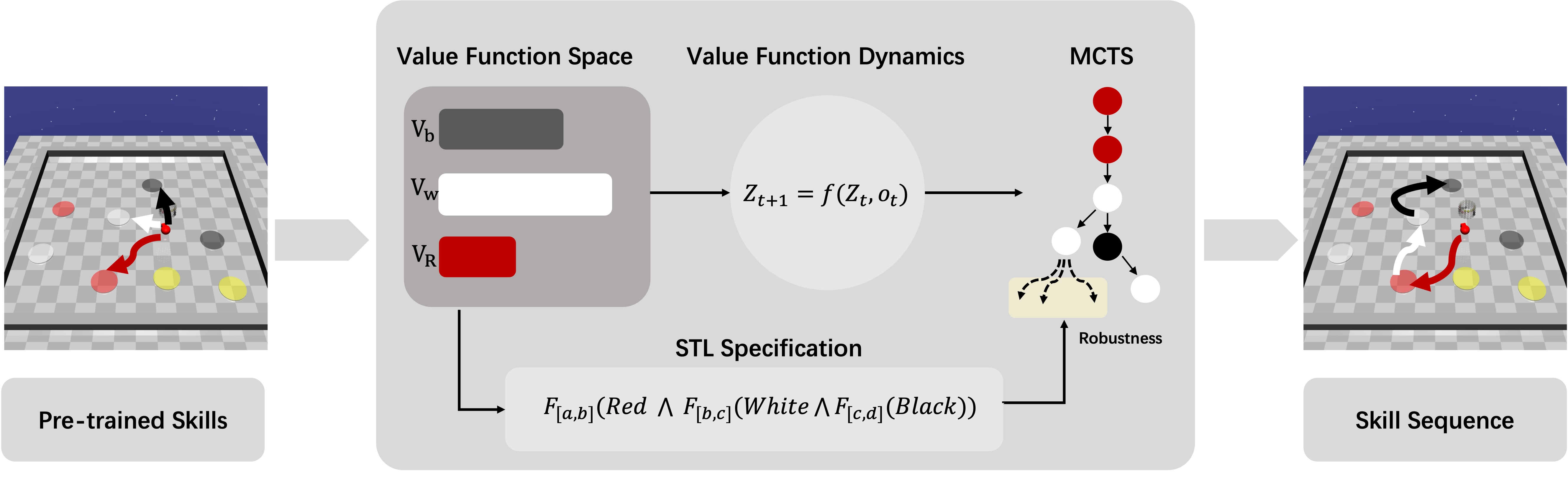
Initially, we obtain a set skills through goal-conditioned actor-critic RL, where each skill is associated with a distinct task. These skills’ value functions are then stacked, creating a value function space that abstracts the original state space to a dimensionality corresponding to the number of tasks, effectively reducing the complexity of the state representation. Next, we employ supervised learning to model the dynamics within this value function space [19], capturing the essential transitions between tasks. With the dynamics model, we frame an optimization problem that incorporates these value function dynamics alongside STL to articulate the tasks’ requirements. We approximate the robustness value using value functions as predicates. To solve this optimization problem and determine the optimal sequence of skills, we utilize Monte Carlo Tree Search (MCTS) [21], leveraging its exploratory capabilities to navigate the space of possible skill sequences efficiently.
IV-B Value Function Space Dynamics
Given an environment MDP where is a set of states, is a set of actions, is the transition function and is the immediate reward (may adjust according to the skill we want to obtain). We can define another MDP with a finite set of k skills trained with sparse outcome rewards in and their corresponding value functions . By constructing an embedding space Z by stacking these skill value functions, we obtain an abstract representation that maps a state to a k-dimensional representation , which called the Value Function Space (VFS). This representation effectively captures functional information regarding the full range of interactions that the agent can engage in with the environment through the execution of skills, making it a scalable state abstraction for subsequent tasks. Further, we can learn a transition dynamics such that via supervised learning using a dataset of prior interactions in the environment. Depending on the high level task, we will adjust the reward accordingly using STL.
IV-C Optimization with VFSTL
Given the forward system dynamic , a goal latent state , and a scoring function for the high-level task, we can formulate a general optimization problem [8] that obtain by solving the following optimization problem:
| (3) | ||||
| s.t. |
, this cost function can be represent by any STL formula.
Thus, we can formulate equation (3) with STL and solve it for long-horizon task planning. For example, suppose we place a blue ball and a red in an interactive environment. Then we train two policies, one for reaching the blue ball and one for reaching the red ball . It is easy to obtain the VFS at the red ball and the blue ball . Suppose we want the agent reach the red ball first and then reach the blue ball, we can formulate following problem:
| (4) |
set of skills
IV-D Monte-Carlo Tree Search
Given that the forward dynamic is nonlinear and non-convex, it can not be linearized due to nature of neural network. We attempt to solve the optimization problem with model-based RL Algorithm 1. Our approach involves the MCTS to identify the optimal skill sequence for maximizing the robustness value of STL specifications that define specific long-horizon tasks shown in Algorithm 2.
Within each iteration of MCTS, nodes are selected based on the upper confidence bound (UCB) formula, represented by the equation
| (5) |
where the term is initialized to 0 and is subsequently updated following the completion of simulations and the receipt of rewards from the robustness value of the STL . Additionally, denotes the number of visits to the current node, refers to the parent node of , and represents a constant parameter that balances the trade-off between exploration and exploitation (Line 23).
The algorithm then proceeds to expand the tree by adding child node if the nodes has not been visited (Line 19), conducts playout simulations to assess potential game outcomes based on the robustness of the STL task formulation (Line 14), and subsequently backpropagates the results to update all parents statistics of the nodes (Line 24). This iterative process is repeated until a specified computational budget is reached (Line 1).
Ultimately, the selection of the skill sequence involves navigating the tree from the root and identifying the skill that leads to the child node with the highest .

V Experiments
In this section, we introduce the experimental setup, training details for skills and dynamics, and simulation results. Upon learning the skills and dynamics, we demonstrate that our method, without further training, can fulfill various tasks, including sequencing, reach-avoid, and stability, using only raw observations from onboard sensors. We also present randomly generated Signal Temporal Logic (STL) formulas to illustrate that utilizing the value function as predicates effectively approximates the ground truth robustness value, computed using privileged information.
V-A Simulation Environment
Our simulation environment is defined in safety-gym[18] based on mujoco[24]. It includes a robot agent and eight goal regions defined with four different colors: gray, red, yellow and white as shown in Fig. 2. The agent is a differential wheel robot equipped with proprioceptive sensors capable of capturing velocities and accelerations of internal states. Additionally, it includes a LiDAR capable of obtaining a 2D point cloud of the target regions.
V-B Skills and Value Function Dynamics Training
Since the training of skills is not the main topic of this work and for the ease of comparison, we use the pre-trained skills from LTLGC[15] directly. There are four skills responsible of reaching the four different colors, respectively. They are trained with the Proximal Policy Optimization (PPO) in a goal-conditioned fashion, which means the reward is +1 if and only the agent reaches the target region, while for any other states, the reward is 0. The PPO method trains a policy network and a value function network who are two different Multi-Layer Perceptrons (MLPs) here [16]. They share the same input structure which consists of the current goal representation , internal states and the point cloud from LiDAR . The output of the policy MLP is a integer indicating one of the primitive actions: turn left, turn right, move forward and move backward. While, the output of the value function MLP is the expected future reward following the current policy, which also means the possibility of reaching the target region.
Remark: It worth noted that, our method dose not depend one how the skill is trained, as long as we can get a critic of the skill.
The dynamic model predicts the value function values of the next time step, abbreviated as values, given the current values and the activated skill . Here, the time step is 1 in the value function space. However, it could be any time step in the low-level MDP, that is the happens after executing for time steps in the environment. Smaller means more restiveness, but more time steps. Here we choose for the balance of restiveness and computation.
The architecture of our dynamic network is as 3 layer MLP with ReLU activation function. To train it, for each epoch, we randomly execute policies for steps and totally 1,000 steps in the environment. During epochs the positions of the robot and goal regions are randomly initialized. Finally, we record 10,000 pair of . Then we compute the cost using mean square error and then use Adam optimizer to train the network.
V-C Simulation Results
Given the trained skills and dynamics, we then solve the problem using model predictive controller i.e. recompute skill sequence produced by MCTS every 2 steps. The rollout score in MCTS is the STL robustness computed using RTMAT [13]. As shown in the Fig. 3, our method can successfully satisfy sequencing, reach-avoid and stability tasks. And the sequencing task describe that the robot needs to first visit a red region, then a jet-black region in two steps, finally a red region 3(a). The agent then operates randomly, as it already satisfies the specification. Fig. 3(b) shows the reach-avoid case, the task is to visit a jet-black region, avoid yellow regions, and aftermath the agent should visit a red region and avoid yellow regions. The stable task is simply to reach red regions and stay there until termination Fig. 3(c).
V-D Robustness Representation
In the experiment, we to explore the correlation between path robustness in value function space and its translation to robustness within a simulation environment’s state space. To conduct this exploration, we considered three distinct navigational tasks: reach-avoid, chain, and stale. For each of these task classifications, we procedurally generated a suite of 100 random signal temporal logic formulations. The reach-avoid task was characterized by the necessity to approach certain states while avoid other states. The chain task entailed a sequence of state visits, with the order of these visits being strictly defined. For the stable task, the objective was to attain a specific state and sustain presence within that state. The is set to 100, each skill in generated skill sequence will be executed in the simulation environment for 100 time step, and total horizon will be set to 10, totally 10 skills will be sequenced to solve the task.
Firstly, we calculated the robustness of the paths within the value function space—a theoretical construct that provides an abstract measure of task fulfillment. Secondly, we assessed the robustness in the state space of the simulation environment, employing Euclidean distance as a practical metric to ascertain whether the tasks were satisfied within a simulated real-world scenario.
Our primary hypothesis posited that the robustness measure obtained in the value function space would be indicative of the robustness in the state space. We anticipated that planning within the value function space would effectively guide successful planning within the state space. To evaluate task completion, we established that a robustness score greater than zero would signify a successfully completed task, whereas a score less than zero would indicate failure.
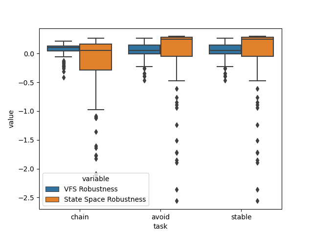
The experiment result is shown in Fig. 4. For all three tasks reach-avoid, chain, and stable, the lower quartile of robustness scores in the value function space were all above zero. This suggests that in the value function space, the tasks achieved a success rate of at least , indicating a generally effective path generation by the MCTS algorithm.
In the state space, a similar level of success was observed for the reach-avoid and stable tasks, where the lower quartile of robustness scores also remained above zero. This alignment demonstrates that planning within the value function space can indeed translate effectively into state space for these two types of tasks, supporting our hypothesis.
However, a slight deviation was encountered in the chain task’s performance. The lower performance is attributable to the complexity of the task, which involves completing a sequence of subtasks within a limited time horizon. The controller is sometimes required to transition to the next subtask before the current goal is fully achieved, to optimize for the overall STL robustness. This aspect is visually represented in the provided figures, which also highlight several outliers with subpar performance.
The outliers are indicative of the limitations in the quality of the policy trained via reinforcement learning. While the value function robustness scores are clustered around zero, an effort to maximize STL compliance, the corresponding robustness in the state space exhibited more negative values. This discrepancy underscores a deficiency in the policy’s ability to navigate the agent to the desired positions within the environment, resulting in a divergence between the theoretical robustness of the value function and the practical robustness observed in the state space.
VI CONCLUSIONS
This paper presented VFSTL, a novel model-based RL framework that leverages pre-trained RL policies to satisfy desired unseen STL specifications for robot planning tasks. By abstracting the state space into value function spaces, we computes and predicts robustness values of STL directly from onboard sensor data. Our method no longer requires hand-crafted predicates of STL and scales well with a large amount of existing trained policies for planning. Apart from theoretical analysis, simulation results also validated the soundness and applicability of our framework. For future research directions, we plan to consider online assessment STL robustness measures to facilitate early pruning of low-potential branches, thereby accelerating the search process. Additionally, we also aim to extend our method into the decentralized setting and decompose the global STL specification into several local formulas for individual agents.
References
- [1] Marcin Andrychowicz, Filip Wolski, Alex Ray, Jonas Schneider, Rachel Fong, Peter Welinder, Bob McGrew, Josh Tobin, OpenAI Pieter Abbeel, and Wojciech Zaremba. Hindsight experience replay. Advances in neural information processing systems, 30, 2017.
- [2] Brandon Araki, Xiao Li, Kiran Vodrahalli, Jonathan DeCastro, Micah Fry, and Daniela Rus. The logical options framework. In International Conference on Machine Learning, pages 307–317. PMLR, 2021.
- [3] Christel Baier and Joost-Pieter Katoen. Principles of model checking. MIT press, 2008.
- [4] Calin Belta and Sadra Sadraddini. Formal methods for control synthesis: An optimization perspective. Annual Review of Control, Robotics, and Autonomous Systems, 2:115–140, 2019.
- [5] Mohammadhosein Hasanbeig, Alessandro Abate, and Daniel Kroening. Logically-constrained reinforcement learning. arXiv preprint arXiv:1801.08099, 2018.
- [6] Roland B Ilyes, Qi Heng Ho, and Morteza Lahijanian. Stochastic robustness interval for motion planning with signal temporal logic. In 2023 IEEE International Conference on Robotics and Automation (ICRA), pages 5716–5722. IEEE, 2023.
- [7] Parv Kapoor, Anand Balakrishnan, and Jyotirmoy V Deshmukh. Model-based reinforcement learning from signal temporal logic specifications. arXiv preprint arXiv:2011.04950, 2020.
- [8] Donald E Kirk. Optimal control theory: an introduction. Courier Corporation, 2004.
- [9] Karen Leung and Marco Pavone. Semi-supervised trajectory-feedback controller synthesis for signal temporal logic specifications. In 2022 American Control Conference (ACC), pages 178–185. IEEE, 2022.
- [10] Xiao Li, Yao Ma, and Calin Belta. A policy search method for temporal logic specified reinforcement learning tasks. In 2018 Annual American Control Conference (ACC), pages 240–245. IEEE, 2018.
- [11] Minghuan Liu, Menghui Zhu, and Weinan Zhang. Goal-conditioned reinforcement learning: Problems and solutions. arXiv preprint arXiv:2201.08299, 2022.
- [12] Yue Meng and Chuchu Fan. Signal temporal logic neural predictive control. IEEE Robotics and Automation Letters, 2023.
- [13] Dejan Ničković and Tomoya Yamaguchi. Rtamt: Online robustness monitors from stl. In International Symposium on Automated Technology for Verification and Analysis, pages 564–571. Springer, 2020.
- [14] Aniruddh G Puranic, Jyotirmoy V Deshmukh, and Stefanos Nikolaidis. Signal temporal logic-guided apprenticeship learning. arXiv preprint arXiv:2311.05084, 2023.
- [15] Wenjie Qiu, Wensen Mao, and He Zhu. Instructing goal-conditioned reinforcement learning agents with temporal logic objectives. Advances in Neural Information Processing Systems, 36, 2024.
- [16] Antonin Raffin, Ashley Hill, Adam Gleave, Anssi Kanervisto, Maximilian Ernestus, and Noah Dormann. Stable-baselines3: Reliable reinforcement learning implementations. Journal of Machine Learning Research, 22(268):1–8, 2021.
- [17] Vasumathi Raman, Alexandre Donzé, Mehdi Maasoumy, Richard M Murray, Alberto Sangiovanni-Vincentelli, and Sanjit A Seshia. Model predictive control with signal temporal logic specifications. In 53rd IEEE Conference on Decision and Control, pages 81–87. IEEE, 2014.
- [18] Alex Ray, Joshua Achiam, and Dario Amodei. Benchmarking safe exploration in deep reinforcement learning. arXiv preprint arXiv:1910.01708, 7(1):2, 2019.
- [19] Dhruv Shah, Peng Xu, Yao Lu, Ted Xiao, Alexander Toshev, Sergey Levine, and Brian Ichter. Value function spaces: Skill-centric state abstractions for long-horizon reasoning. arXiv preprint arXiv:2111.03189, 2021.
- [20] Daqian Shao and Marta Kwiatkowska. Sample efficient model-free reinforcement learning from ltl specifications with optimality guarantees. arXiv preprint arXiv:2305.01381, 2023.
- [21] David Silver, Thomas Hubert, Julian Schrittwieser, Ioannis Antonoglou, Matthew Lai, Arthur Guez, Marc Lanctot, Laurent Sifre, Dharshan Kumaran, Thore Graepel, et al. Mastering chess and shogi by self-play with a general reinforcement learning algorithm. arXiv preprint arXiv:1712.01815, 2017.
- [22] Richard S Sutton, Doina Precup, and Satinder Singh. Between mdps and semi-mdps: A framework for temporal abstraction in reinforcement learning. Artificial intelligence, 112(1-2):181–211, 1999.
- [23] Gerald Tesauro et al. Temporal difference learning and td-gammon. Communications of the ACM, 38(3):58–68, 1995.
- [24] Emanuel Todorov, Tom Erez, and Yuval Tassa. Mujoco: A physics engine for model-based control. In 2012 IEEE/RSJ international conference on intelligent robots and systems, pages 5026–5033. IEEE, 2012.
- [25] Pashootan Vaezipoor, Andrew C Li, Rodrigo A Toro Icarte, and Sheila A Mcilraith. Ltl2action: Generalizing ltl instructions for multi-task rl. In International Conference on Machine Learning, pages 10497–10508. PMLR, 2021.
- [26] Yanwei Wang, Nadia Figueroa, Shen Li, Ankit Shah, and Julie Shah. Temporal logic imitation: Learning plan-satisficing motion policies from demonstrations. arXiv preprint arXiv:2206.04632, 2022.
- [27] Tichakorn Wongpiromsarn, Ufuk Topcu, and Richard M Murray. Receding horizon control for temporal logic specifications. In Proceedings of the 13th ACM international conference on Hybrid systems: computation and control, pages 101–110, 2010.