Construction of a curved Kakeya set

Abstract.

We construct a compact set in $\mathbb{R}^{2}$ of measure $0$ containing a piece of a parabola of every aperture between $1$ and $2$. As a consequence, we improve lower bounds for the $L^{p}$-$L^{q}$ norm of the corresponding maximal operator for a range of $p,q$. Moreover, our construction can be generalised from parabolas to a family of curves with cinematic curvature.

1. Introduction

Consider Wolff’s circular maximal Kakeya function introduced in [KW99]:

$$\mathcal{C}f(r)=\sup_{x\in\mathbb{R}^{2}}\int_{C(x,r)}|f(y)|dy,$$

initially defined for continuous functions $f:\mathbb{R}^{2}\to\mathbb{C}$ with compact support, where $r\in[1,2]$ and $C(x,r)$ denotes the circle centred at $x$ of radius $r$. For $\delta>0$, we can also consider a $\delta$-thickened version of the maximal function, defined by

$$\mathcal{C}_{\delta}f(r)=\sup_{x\in\mathbb{R}^{2}}\frac{1}{|C_{\delta}(x,r)|}\int_{C_{\delta}(x,r)}|f(y)|dy,$$

where $C_{\delta}(x,r)$ denotes the annulus centred at $x$ of radius $r$ and thickness $\delta$, namely, $C_{\delta}(x,r)=\{y\in\mathbb{R}^{2}:r-\delta\leq|y-x|\leq r+\delta\}$. For Lebesgue exponents $p,q\in[1,\infty]$, we are interested in the $L^{p}(\mathbb{R}^{2})\to L^{q}([1,2])$ mapping property of $\mathcal{C}$ and $\mathcal{C}_{\delta}$. Wolff [Wol97] proved the bound

$$\left\lVert\mathcal{C}_{\delta}\right\rVert_{L^{3}\to L^{3}}\lesssim_{\varepsilon}\delta^{-\varepsilon},\quad\forall\varepsilon>0,$$

which is sharp except for the $\varepsilon$-loss. Using this, he concluded that every compact subset of $\mathbb{R}^{2}$ containing a circle of every radius between $1$ and $2$ must have Hausdorff dimension $2$.

A closely related analogue of $\mathcal{C}$ is a parabolic maximal function defined by

$$\mathcal{P}f(a)=\sup_{(x_{1},x_{2})\in\mathbb{R}^{2}}\int_{0}^{1}|f(x_{1}+t,x_{2}+at^{2})|dt.$$

Similarly, for each $\delta>0$, we can define the $\delta$-thickened version

$$\mathcal{P}_{\delta}f(a)=\sup_{(x_{1},x_{2})\in\mathbb{R}^{2}}(2\delta)^{-1}\int_{0}^{1}\int_{-\delta}^{\delta}|f(x_{1}+t,x_{2}+at^{2}+s)|dsdt.$$

1.1. Curves of cinematic curvature

Both maximal functions can be thought of as special cases of a family of curves with cinematic curvature, introduced by Sogge [Sog91]. See also [KW99][Zah12a][Zah12b][PYZ22][CGY23] [Zah23][CG24] for related discussions on maximal operator bounds related to curves of cinematic curvature. There are many different but essentially equivalent formulations of a family of curves $u_{a}(t)$ satisfying the cinematic curvature condition; for instance, in [CGY23] it is formulated as

$$\det\begin{bmatrix}u_{tt}&u_{at}\\ u_{ttt}&u_{att}\end{bmatrix}\neq 0,$$ (1.1)

which one can check to be true for the family of parabolas $\{(t,at^{2}):t\in[0,1]\}$ with $a\in[1,2]$.

Thus, one has the following upper bounds for the parabolic maximal operator.

$$\left\lVert\mathcal{P}_{\delta}f\right\rVert_{L^{3}([1,2])}\lesssim_{\varepsilon}\delta^{-\varepsilon}\left\lVert f\right\rVert_{L^{3}(\mathbb{R}^{2})}\quad\forall\varepsilon>0,$$ (1.2)

$$\left\lVert\mathcal{P}_{\delta}f\right\rVert_{L^{q}([1,2])}\lesssim\delta^{\frac{1}{2}-\frac{3}{2p}}\left\lVert f\right\rVert_{L^{p}(\mathbb{R}^{2})},\quad p<\frac{8}{3},\quad q\geq\frac{2p}{p-1}.$$ (1.3)

Indeed, (1.2) follows from [Zah12a] or [Zah12b], and (1.3) follows from [KW99]. It is worth noting that (1.3) has no $\varepsilon$-losses in the power of $\delta$.

1.2. Lower bounds

In order to make things simple, we first restrict ourselves to the parabolic maximal operator $\mathcal{P}_{\delta}$. Define

$$B(p,q)=\sup_{f\neq 0}\frac{\left\lVert\mathcal{P}f\right\rVert_{L^{q}([1,2])}}{\left\lVert f\right\rVert_{L^{p}(\mathbb{R}^{2})}},\quad B(p,q,\delta)=\sup_{f\neq 0}\frac{\left\lVert\mathcal{P}_{\delta}f\right\rVert_{L^{q}([1,2])}}{\left\lVert f\right\rVert_{L^{p}(\mathbb{R}^{2})}}.$$

The inequalities (1.2) and (1.3) give upper bounds for $B(p,q,\delta)$. On the other hand, the existence of some Kakeya sets provides some related lower bounds of $B(p,q,\delta)$. For clarity, we first introduce the notion of (vertical) $\delta$-thickening $S(\delta)$ for a subset $S\subseteq\mathbb{R}^{2}$:

$$S(\delta):=\{x+(0,\varepsilon):x\in S,-\delta\leq\varepsilon\leq\delta\}.$$ (1.4)

Theorem 1.1 (Parabolic variant of Kolasa-Wolff construction [KW99]).

There exists a compact subset $K$ of $\mathbb{R}^{2}$ of Lebesgue measure $0$ that contains a piece of length $\sim 1$ of a parabola of every aperture between $1$ and $2$. Moreover, its $\delta$-thickening $K(\delta)$ has measure $\lesssim(\log\delta^{-1})^{-2}(\log\log\delta^{-1})^{2}$. Thus we have the lower bound

$$B(p,q,\delta)\gtrsim(\log\delta^{-1})^{2/p}(\log\log\delta^{-1})^{-2/p},$$ (1.5)

where the implicit constant is independent of $\delta$. In particular, $B(p,q)=\infty$ if $p<\infty$.

Proof.

This follows from an easy adaptation of the main construction of Proposition 1.1 in [KW99] for circles to the case of parabolas. ∎

We also encourage the reader to check other curved Kakeya set constructions, such as [BR68][Kin68][Dav72][Tal80][HKLO23][CYZ23].

The main theorem of this paper is an improvement of Theorem 1.1 as follows.

Theorem 1.2 (Main theorem).

There exists a compact subset $K$ of $\mathbb{R}^{2}$ of Lebesgue measure $0$ that contains a piece of length $\sim 1$ of a parabola of every aperture between $1$ and $2$. Moreover, its $\delta$-thickening $K(\delta)$ has measure $\lesssim(\log\delta^{-1})^{-2}$. Thus we have the lower bound

$$B(p,q,\delta)\gtrsim(\log\delta^{-1})^{2/p}.$$ (1.6)

Namely, by refining the main construction in [KW99], we are able to remove the $\log\log\delta^{-1}$ factor in the lower bound.

1.3. Kakeya set with cinematic curvature

More generally, we can generalise the construction in Theorem 1.2 with parabolas replaced by a family of functions obeying cinematic curvature conditions.

We start with a $C^{2}$-function $f:[0,1]\to\mathbb{R}$ that satisfies the following assumptions:

$$f^{\prime}(0)\geq 0,\quad\inf f^{\prime\prime}>0,$$ (1.7)

$$f^{\prime\prime\prime}\text{ exists and is bounded in }(0,1),$$ (1.8)

$$f^{\prime}f^{\prime\prime\prime}-(f^{\prime\prime})^{2}\leq 0\text{ in }(0,1).$$ (1.9)

Then one can check that the family of functions $u_{a}(t)=af(t)$, $1\leq a\leq 2$ satisfies (1.1). Also, the case of parabolas corresponds to $f(t)=t^{2}$.

Define the corresponding maximal operators as

$$\mathcal{R}g(a) =\sup_{(x_{1},x_{2})\in\mathbb{R}^{2}}\int_{0}^{1}|g(x_{1}+t,x_{2}+af(t))|dt$$ (1.10)

$$\mathcal{R}_{\delta}g(a) =\sup_{(x_{1},x_{2})\in\mathbb{R}^{2}}(2\delta)^{-1}\int_{0}^{1}\int_{-\delta}^{\delta}|g(x_{1}+t,x_{2}+af(t)+s)|dsdt,$$

and define the corresponding operator norms

$$R(p,q)=\sup_{g\neq 0}\frac{\left\lVert\mathcal{R}g\right\rVert_{L^{q}([1,2])}}{\left\lVert g\right\rVert_{L^{p}(\mathbb{R}^{2})}},\quad R(p,q,\delta)=\sup_{g\neq 0}\frac{\left\lVert\mathcal{R}_{\delta}g\right\rVert_{L^{q}([1,2])}}{\left\lVert g\right\rVert_{L^{p}(\mathbb{R}^{2})}}.$$

Theorem 1.3.

Let $f:[0,1]\to\mathbb{R}$ be a $C^{2}$ function obeying (1.7)(1.8)(1.9). Then there exists a compact subset $K$ of $\mathbb{R}^{2}$ of Lebesgue measure $0$ that contains a translated copy of a piece of length $\sim 1$ of the graph of a function of the form $af(x)$ where $1\leq a\leq 2$. Moreover, its $\delta$-thickening $K(\delta)$ has measure $\lesssim(\log\delta^{-1})^{-2}$. Thus we have the lower bound

$$R(p,q,\delta)\gtrsim(\log\delta^{-1})^{2/p}.$$ (1.11)

In particular, $R(p,q)=\infty$ for $p<\infty$.

In the following of this article, we prove Theorem 1.3, from which Theorem 1.2 follows as a corollary.

1.4. Outline of the article

In Section 2 we construct the $M$-th stage $K_{M}$ of the curved Kakeya set $K$. In Section 3 we iterate the previous construction to obtain an actual curved Kakeya set of zero measure. In the appendix we give a brief summary of current best upper and lower bounds for $R(p,q,\delta)$.

1.5. Acknowledgements

Tongou Yang is supported by the Croucher Fellowships for Postdoctoral Research. Yue Zhong is supported in part by the National Key R&D Program of China (No. 2022YFA1005700) and the NNSF of China (No. 12371105). Both authors would like to thank Sanghyuk Lee and Shaoming Guo for bringing this problem to our attention, and Lixin Yan, Xianghong Chen and Mingfeng Chen for helpful suggestions.

2. Compression by forcing tangencies

Let $M\in 2\mathbb{N}$ be large enough. In this section, we are going to present the $M$-th building block $F_{M}$ of the construction of the curved Kakeya set $K$ in Theorem 1.3. This is done using a “cut-and-slide” procedure. The idea at each step $j$ is to create many tangencies at a fixed $x$-coordinate $x_{j}$ by translations, so that the curved rectangles are compressed near $x_{j}$. The following is the precise construction.

Unless otherwise specified, all implicit constants are allowed to depend on $f$ only; more precisely, they depend on $\left\lVert f\right\rVert_{C^{2}}$, $\inf f^{\prime\prime}$ and $\sup|f^{\prime\prime\prime}|$ given in (1.7)(1.8)(1.9).

2.1. Step 0

We start with a $C^{2}$-function $f:[0,1]\to\mathbb{R}$ obeying (1.7)(1.8) (1.9). Fix $1\leq a_{0}\leq 2$ and $0<\delta_{0}\leq 2-a_{0}$. Consider the initial “curved rectangle”

$$T^{(0)}(a_{0},\delta_{0}):=\{(x,af(x)):x\in[0,1],a\in[a_{0},a_{0}+\delta_{0}]\}.$$ (2.1)

Fix $M\in 4\mathbb{N}$. We divide $T_{0}(a_{0},\delta_{0})$ into $2^{M}$ “curved rectangles” of the form

$$T^{(0)}_{n}:=T^{(0)}(a_{0}+n\delta_{0}2^{-M},\delta_{0}2^{-M}),\quad n=0,1,\dots,2^{M}-1.$$ (2.2)

The curve at the bottom of $T^{(0)}_{n}$ is given by

$$L^{(0)}_{n}(x):=a_{0}f(x).$$ (2.3)

Partition $[0,1]$ uniformly into $M/2$ intervals of length $2M^{-1}$, where the partitioning points are given by

$$x_{j}:=2jM^{-1},\quad j=0,1,\dots,M/2.$$ (2.4)

2.2. Step 1

For odd $n=1,3,\dots,2^{M}-1$, we now apply different translations to $T^{(0)}_{n}$ so that its bottom curve $L^{(0)}_{n}$ will be tangent to the bottom curve $L^{(0)}_{n-1}$ at $x_{1}$. That is, we need to find translations $u:=u_{n}^{(1)}$, $v:=v_{n}^{(1)}$ such that

$$\left\{\begin{aligned} &af(x_{1}-u)+v=\tilde{a}f(x_{1})\\ &af^{\prime}(x_{1}-u)=\tilde{a}f^{\prime}(x_{1})\\ \end{aligned}\right.$$

where $a=a_{0}+n\delta_{0}2^{-M}$ and $\tilde{a}=a_{0}+(n-1)\delta_{0}2^{-M}$.

To find the solutions, we first focus on the second equation. First, using the implicit function theorem and the fact that $\inf f^{\prime\prime}>0$, we see that for $M$ large enough, such $u$ always exists and $0<u\lesssim\delta_{0}2^{-M}$. To find the expression of $u$, by the mean value theorem, there exists some $\xi=\xi_{n}^{(1)}$ such that

$$f^{\prime}(x_{1})-f^{\prime}(x_{1}-u)=uf^{\prime\prime}(\xi).$$

Moreover, such $\xi$ must be unique since $f^{\prime\prime}>0$. Thus the second equation gives

$$u=u_{n}^{(1)}=\frac{\delta_{0}2^{-M}}{a}\frac{f^{\prime}(x_{1})}{f^{\prime\prime}(\xi)}.$$ (2.5)

Plugging into the first equation, we can find $v$, which is also positive. Also, by Lemma 2.1 below, the translated curve $L_{n}^{(0)}+(u,v)$ is still strictly above $L_{n-1}^{(0)}$ except at the tangent point.

After Step 1, we obtain $2^{M-1}$ larger curved figures

$$T^{(1)}_{n}:=T_{n}^{(0)}\bigcup(T_{n+1}^{(0)}+(u_{n+1}^{(1)},v_{n+1}^{(1)})),$$ (2.6)

where $n=0,2,\dots,2^{M}-2$, that are compressed well at $x_{1}$. Moreover, for each even $n$, the curve $L_{n}^{(0)}$ is still the bottom curve of $T^{(1)}_{n}$. Denote

$$T^{(1)}:=\bigcup_{n:2|n}T^{(1)}_{n}.$$

2.3. Step $2$

We continue in a similar way, this time compressing $T^{(1)}_{n}$, $n=0,2,\dots,2^{M}-2$ at the point $x_{2}$. More precisely, for $n=2,6,10,\dots,2^{M}-2$, we translate $T^{(1)}_{n}$ further by some $(u_{n}^{(2)},v_{n}^{(2)})$ so that its bottom curve $L_{n}^{(0)}$ is tangent to $L^{(0)}_{n-2}$ at $x_{2}$. Similarly to (2.6), we obtain $2^{M-2}$ larger curved figures $T^{(2)}_{n}$, $n=0,4,\dots,2^{M}-4$, whose bottom curve is $L_{n}^{(0)}$ by Lemma 2.1 below, and they are compressed well at $x_{2}$. Denote

$$T^{(2)}:=\bigcup_{n:4|n}T^{(2)}_{n}.$$

Refer to Figure 1, which shows two steps of translations when $2^{M}=16$.

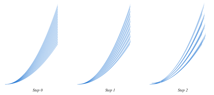
Figure 1. Figure after two steps when $2^{M}=16$

2.4. Step $j$

Now we describe a general Step $j$. For each $n$ of the form $2^{j}k+2^{j-1}$, $k=0,1,\dots,2^{M-j}-1$, we translate $T_{n}^{(j-1)}$ by some $(u^{(j)}_{n},v^{(j)}_{n})$ so that its bottom curve $L^{(0)}_{n}$ is tangent to $L_{n-2^{j-1}}^{(0)}$ at $x_{j}$. By the same computation as in Step 1, we have

$$u_{n}^{(j)}=\frac{\delta_{0}2^{j-1-M}}{a}\frac{f^{\prime}(x_{j})}{f^{\prime\prime}(\xi)},$$ (2.7)

where $a=a_{0}+n\delta_{0}2^{-M}$, and $\xi=\xi_{n}^{(j)}$ is the unique number such that

$$f^{\prime\prime}(\xi)=\frac{f^{\prime}(x_{j})-f^{\prime}(x_{j}-u^{(j)}_{n})}{u^{(j)}_{n}},$$ (2.8)

and its existence is guaranteed by the implicit function theorem. Moreover, a direct computation using Taylor’s theorem gives for some $\zeta=\zeta_{n}^{(j)}$ that

$$v_{n}^{(j)}=\delta_{0}2^{j-1-M}\left[\frac{f^{\prime}(x_{j})^{2}}{f^{\prime\prime}(\xi)}-f(x_{j})\right]-a\frac{f^{\prime\prime}(\zeta)}{2}(u_{n}^{(j)})^{2}.$$ (2.9)

Thus, similarly to (2.6), we obtain $2^{M-j}$ larger curved figures $T_{n}^{(j)}$, $n=0,2^{j},\dots,2^{M}-2^{j}$, which are compressed well at $x_{j}$. Also, by the following lemma, the bottom of $T_{n}^{(j)}$ is still $L_{n}^{(0)}$. Denote

$$T^{(j)}:=\bigcup_{n:2^{j}|n}T^{(j)}_{n}.$$

Lemma 2.1.

If $f:[0,1]\to\mathbb{R}$ is a $C^{2}$ function obeying (1.7)(1.8)(1.9), $x_{0}\in[0,1]$, and $(u,v)$ is the solution of the equation $\left\{\begin{aligned} &af(x_{0}-u)+v=\tilde{a}f(x_{0})\\ &af^{\prime}(x_{0}-u)=\tilde{a}f^{\prime}(x_{0})\\ \end{aligned},\right.$ then we have $af(x-u)+v\geq\tilde{a}f(x)$ for any $x$ while $a\geq\tilde{a}$ (such that $u,v$ exist).

Proof.

Fix $\tilde{a},x,x_{0}$. Let

$$F(a)=a(f(x-u(a))-f(x_{0}-u(a)))-\tilde{a}(f(x)-f(x_{0})),$$

where we regard $u,v$ as functions of $a$. We have $F(\tilde{a})=0$ since $u(\tilde{a})=v(\tilde{a})=0$. We want to show $F(a)\geq 0$ while $a\geq\tilde{a}$, and it suffices to show that $F^{\prime}(a)\geq 0$ for $a\geq\tilde{a}$.

Since $u$ is the solution of the equation $af^{\prime}(x_{0}-u)=\tilde{a}f^{\prime}(x_{0})$, we have

$$\frac{\partial}{\partial a}(af^{\prime}(x_{0}-u))=\frac{\partial}{\partial a}(\tilde{a}f^{\prime}(x_{0})),$$

which means that

$$u^{\prime}(a)=\frac{f^{\prime}(x_{0}-u)}{af^{{}^{\prime\prime}}(x_{0}-u)}.$$

Denote $X=x-u$ and $X_{0}=x_{0}-u$. Then by direct computation,

$$F^{\prime}(a) =(f(X)-f(X_{0}))-a(f^{\prime}(X)-f^{\prime}(X_{0}))\cdot u^{\prime}(a)$$

$$=\dfrac{(f(X)-f(X_{0}))f^{\prime\prime}(X_{0})-(f^{\prime}(X)-f^{\prime}(X_{0}))f^{\prime}(X_{0})}{f^{\prime\prime}(X_{0})}$$

$$=\frac{G(X)-G(X_{0})}{f^{\prime\prime}(X_{0})},$$

where we have denoted

$$G(X):=f(X)f^{\prime\prime}(X_{0})-f^{\prime}(X)f^{\prime}(X_{0}).$$

Then it suffices to show $G(X)\geq G(X_{0})$ for all $X$, which is true if we can show $G^{\prime}(X)\geq 0$ for $X\geq X_{0}$ and $G^{\prime}(X)\leq 0$ for $X\leq X_{0}$. To this end, we consider

$$H(X):=\frac{G^{\prime}(X)}{f^{\prime}(X)}=\frac{f^{\prime}(X)f^{\prime\prime}(X_{0})-f^{\prime\prime}(X)f^{\prime}(X_{0})}{f^{\prime}(X)}.$$

We note that $X=x-u>0$ since $x\geq 2/M\ll u$. Thus by (1.7), $f^{\prime}(X)>0$. Thus it suffices to show that $H(X)\geq 0$ for $X\geq X_{0}$ and $H(X)\leq 0$ for $X\leq X_{0}$. But $H(X_{0})=0$, so it further suffices to show $H^{\prime}(X)\geq 0$ for all $X$. But direct computation gives

$$H^{\prime}(X)=\frac{f^{\prime}(X_{0})[f^{\prime\prime}(X)^{2}-f^{\prime\prime\prime}(X)f^{\prime}(X)]}{f^{\prime}(X)^{2}},$$

which is nonnegative by (1.9). This finishes the proof. ∎

2.5. End of construction

Denote

$$m:=M/2.$$ (2.10)

We perform the above procedures for $m-1$ times at each tangent point $x_{j}=2j/M$, $j=1,\dots,m-1$, arriving at the set $T^{(m)}$. We now define our required set

$$F_{M}:=T^{(m)}\bigcap\left(\left[\frac{4\log M}{M},1\right]\times\mathbb{R}\right).$$ (2.11)

Note that this means we throw away the part of $T^{(m)}$ over $[0,x_{j}]$ where $j<2\log M$. The choice of the cutoff $\frac{4\log M}{M}$ will be clear later in (2.22) in the proof of Theorem 2.3.

2.6. Computation of translations

Our first task is to control the sum $(u_{n},v_{n})$ of all translations $(u_{n}^{(j)},v_{n}^{(j)})$ that have been performed to the original curved rectangle $T^{(0)}_{n}$ at Steps $j=1,2,\dots,m$.

Given $n=0,1,\dots,2^{M}-1$, by binary expansion, we know there exist unique integers $\varepsilon_{j}=\varepsilon_{j}(n)\in\{0,1\}$, $1\leq j\leq M$ such that $n=\sum_{j=1}^{M}\varepsilon_{j}2^{j-1}$.

For convenience, we introduce the notation

$$\left\lfloor n\right\rfloor_{j}:=n-(n\,\,\mathrm{mod}\,\,2^{j-1}),$$ (2.12)

which means the “integral part” of $n$ in in $2^{j-1}\mathbb{Z}$. Then we note that $\varepsilon_{j}(n)=1$ if and only if $u_{\left\lfloor n\right\rfloor_{j}}$, $v_{\left\lfloor n\right\rfloor_{j}}$ are defined by Step $j$.

Proposition 2.2.

For each $n=0,1,\dots,2^{M}-1$, we have the relations

$$u_{n}=\sum_{j=1}^{m}\varepsilon_{j}(n)u^{(j)}_{\left\lfloor n\right\rfloor_{j}},\quad v_{n}=\sum_{j=1}^{m}\varepsilon_{j}(n)v^{(j)}_{\left\lfloor n\right\rfloor_{j}}.$$ (2.13)

In particular, we have

$$0\leq u_{n}\leq C\delta_{0}2^{-M/2},\quad 0\leq v_{n}\leq C\delta_{0}2^{-M/2}.$$ (2.14)

More generally, denote the partial sums

$$U_{n}^{(j)}:=\sum_{i=1}^{j}\varepsilon_{i}(n)u^{(i)}_{\left\lfloor n\right\rfloor_{i}},\quad V_{n}^{(j)}:=\sum_{i=1}^{j}\varepsilon_{i}(n)v^{(i)}_{\left\lfloor n\right\rfloor_{i}},$$ (2.15)

then we have

$$0\leq U_{n}^{(j)}\leq C\delta_{0}2^{j-M},\quad 0\leq V_{n}^{(j)}\leq C\delta_{0}2^{j-M}.$$ (2.16)

Here $C$ is a large constant depending on $f$ only.

Proof.

The proof of (2.13) is by inspection. For example, if $m>100$ and $n=27$, then $T_{n}^{(0)}$ is translated according to the bottoms of $T_{27}^{(0)}$, $T_{26}^{(0)}$, $T_{24}^{(0)}$ and $T_{16}^{(0)}$ at Steps $1,2,4,5$, respectively; it remains unchanged at all other steps. Note that $\varepsilon_{j}(27)=1$ if and only if $j=1,2,4,5$, whence $27-(27\,\,\mathrm{mod}\,\,2^{j-1})=27,26,24,16$, respectively.

The relations (2.14) then follow from (2.7) and (2.9) and the choice $m=M/2$. The estimates of the partial sums are similar. ∎

This proposition ensures that for large $M$, the total distance of translations is tiny; in particular, it can be less than $\frac{4\log M}{M}$, so that the projections of the translated curved rectangles onto the $x$-axis all contain $[\frac{4\log M}{M},1]$.

For future reference, we denote by $L_{n}$ the bottom curves of $T_{n}^{(0)}$ after all steps of translations. Namely,

$$L_{n}:=L_{n}^{(0)}+(u_{n},v_{n}).$$ (2.17)

2.7. Upper bound of measure

In this subsection, we control the measure of the set $F_{M}$ we constructed.

Theorem 2.3.

The set $F_{M}$ satisfies

$$|F_{M}|\lesssim\delta_{0}M^{-2}.$$ (2.18)

Corollary 2.4.

The lower bound (1.11) holds.

Proof of corollary assuming Theorem 2.3.

Let $\delta=2^{-M}$ and take $g=1_{F_{M}}$ corresponding to $a_{0}=1,\delta_{0}=1$. Then the construction gives $\mathcal{R}_{\delta}g(a)\sim 1$ for every $a\in[1,2]$. Then the result follows from Theorem 2.3. ∎

Proof of Theorem 2.3.

It suffices to show that for each $x_{0}\in[\frac{4\log M}{M},1]$,

$$|\{y\in\mathbb{R}:(x_{0},y)\in F_{M}\}|\lesssim\delta_{0}M^{-2}.$$ (2.19)

Fix $j\in[\log M,m-1]$ and assume $x_{0}\in[x_{j},x_{j+1}]$. For each $n=0,1,\dots,2^{M}-1$, we write

$$n=p+\sum_{i=1}^{j}\varepsilon_{i}\cdot 2^{i-1}\quad(p=0,2^{j},\cdots,2^{M}-2^{j}).$$ (2.20)

In words, for each $j$, we group the translated curved rectangles $T_{n}^{(m)}$ into $2^{M-j}$ groups, and $T_{n}^{(m)}$ belongs to the $p2^{-j}$-th group, whose bottom curve is given by $L_{p}$.

By the triangle inequality, it suffices to show that the thickness of the $p2^{-j}$-th group is $\lesssim\delta_{0}M^{-2}2^{j-M}$. More precisely, we need to show

$$L_{n}(x_{0})-L_{p}(x_{0})+\delta_{0}2^{-M}\lesssim\delta_{0}M^{-2}2^{j-M}.$$ (2.21)

Here, $L_{n}(x_{0})-L_{p}(x_{0})$ is the distance between the bottoms, and $\delta_{0}2^{-M}$ is the thickness of one smallest curved rectangle. But by our choice that $j\geq 2\log M$, we have

$$2^{-M}\lesssim M^{-2}2^{j-M}.$$ (2.22)

Thus our task reduces to showing

$$L_{n}(x_{0})-L_{p}(x_{0})\lesssim\delta_{0}M^{-2}2^{j-M}.$$ (2.23)

We trace back to the configuration right after Step $j$. That is, we let

$$x:=x_{0}-\sum_{i=j+1}^{m-1}u_{\left\lfloor n\right\rfloor_{i}}^{(i)},$$ (2.24)

which lies within $[x_{j-1},x_{j+1}]$, by (2.7). Thus

$$L_{n}(x_{0})-L_{p}(x_{0})=L_{n}^{(j)}(x)-L_{p}^{(j)}(x),$$

where $L_{n}^{(j)}$ stands for the bottom curve of $T_{n}^{(0)}$ after $j$ steps of translations.

Recall that

$$\left\{\begin{aligned} &L_{n}^{(j)}(x)=(a_{0}+\delta_{0}n2^{-M})f(x-U_{n}^{(j)})+V_{n}^{(j)}\\ &L_{p}^{j}(x)=(a_{0}+\delta_{0}p2^{-M})f(x-U_{p}^{(j)})+V_{p}^{(j)}\\ \end{aligned}\right..$$

According to the definition of $U_{n}^{(j)}$ and $V_{n}^{(j)}$, we know that

$$U_{p}^{(j)}=V_{p}^{(j)}=0.$$

We then Taylor expand $f$:

$$f(x-U_{n}^{(j)})=f(x)-f^{\prime}(x)U_{n}^{(j)}+O(U_{n}^{(j)})^{2},$$

and by (2.16), we have $|U_{n}^{(j)}|^{2}\lesssim\delta_{0}^{2}2^{-2j-2M}\ll\delta_{0}M^{-2}2^{j-M}$. Thus we need to show

$$|(a_{0}+\delta_{0}n2^{-M})(f(x)-f^{\prime}(x)U_{n}^{(j)})+V_{n}^{(j)}-(a_{0}+\delta_{0}p2^{-M})f(x)|\lesssim\delta_{0}M^{-2}2^{j-M}.$$ (2.25)

We compute the left hand side using (2.20), (2.15), (2.7) and (2.9):

LHS of (2.25)

$$=\sum_{i=1}^{j}\left(\delta_{0}\varepsilon_{i}2^{i-1-M}f(x)-(a_{0}+\delta_{0}n2^{-M})f^{\prime}(x)u_{\left\lfloor n\right\rfloor_{i}}^{(i)}+v_{\left\lfloor n\right\rfloor_{i}}^{(i)}\right)$$

$$=\delta_{0}2^{-M}\sum_{i=1}^{j}2^{i-1}\left(f(x)-\frac{f^{\prime}(x)f^{\prime}(x_{i})}{f^{\prime\prime}(\xi_{i})}+\frac{f^{\prime}(x_{i})^{2}}{f^{\prime\prime}(\xi_{i})}-f(x_{i})+O(2^{i-M})\right)$$

$$=\delta_{0}2^{-M}\sum_{i=1}^{j}2^{i-1}\left(f(x)-f(x_{i})-(f^{\prime}(x)-f^{\prime}(x_{i}))\frac{f^{\prime}(x_{i})}{f^{\prime\prime}(\xi_{i})}+O(2^{i-M})\right),$$

where we abbreviated $\xi_{i}:=\xi^{(i)}_{\left\lfloor n\right\rfloor_{i}}$. The sum of the quadratic error terms obeys

$$\sum_{i=1}^{j}2^{i-1}2^{i-M}\sim 2^{2j-M}\ll M^{-2}2^{j},$$

so it suffices to prove

$$\sum_{i=1}^{j}2^{i}\left|f(x)-f(x_{i})-(f^{\prime}(x)-f^{\prime}(x_{i}))\frac{f^{\prime}(x_{i})}{f^{\prime\prime}(\xi_{i})}\right|\lesssim 2^{j}M^{-2}.$$ (2.26)

To this end, we fix $i$ and let $g(x)=f(x)-f^{\prime}(x)\frac{f^{\prime}(x_{i})}{f^{\prime\prime}(\xi_{i})}$, so that we need to bound $g(x)-g(x_{i})$. But by direct computation using (1.8),

$$|g^{\prime}(x_{i})|=\left|\frac{f^{\prime}(x_{i})}{f^{\prime\prime}(\xi_{i})}(f^{\prime\prime}(\xi_{i})-f^{\prime\prime}(x_{i}))\right|\lesssim|x-x_{i}|,$$

and so by Taylor expansion of $g$, we have

$$|g(x)-g(x_{i})|\lesssim|x-x_{i}|^{2}.$$

Thus we have reduced the problem to proving

$$\sum_{i=1}^{j}2^{i}|x-x_{i}|^{2}\lesssim 2^{j}M^{-2}.$$

However, using $x\in[x_{j-1},x_{j+1}]$ and the definition that $x_{i}=2i/M$, we obtain the bound. This finishes the proof.

∎

3. Construction of zero measure Kakeya set

In this section, we use a routine method to construct the curved Kakeya set $K$ with zero measure mentioned in Theorem 1.3, based on the sets $F_{M}$ constructed in the previous section.

Start with $T^{(0)}(a_{0}=1,\delta_{0}=1)$ as defined in (2.1). Pick a large integer $M\in 2\mathbb{N}$ such that we have all the results in Section 2. Denote

$$M_{n}:=M^{n}.$$ (3.1)

We then construct the set

$$K_{1}:=F_{M_{1}}=F_{M},$$ (3.2)

which is a compact subset of $[\frac{4\log M}{M},1]\times[-C_{0},C_{0}]$ where $C_{0}=C_{0}(f)$ is a fixed large constant. Denote $A_{1}:=\frac{4\log M}{M}$.

Recall $K_{1}$ consists of $2^{M}$ smaller curved rectangles which we denote by $T(1)$, each of the form $T^{(0)}(a,2^{-M})+(u,v)$ for some $a\in[1,2]$,

$$|u|\leq C2^{-M/2},|v|\leq C2^{-M/2}$$

by (2.14). We then apply the same procedures in Section 2 to each $T(1)$, this time with $a_{0}$ taken to be this $a$, $M$ taken to be $M_{2}$, and $\delta_{0}$ taken to be $2^{-M_{1}}$. (More precisely, to fit the notation of Section 2 perfectly, we should first reverse the translation by $(u_{n},v_{n})$ to $T(1)$, rescale so that it is over $[0,1]$, apply the construction, and then rescale back in the end.) This gives us the set $K_{2}$, whose projection onto the $x$-axis is equal to $[A_{2},1]$ where

$$A_{2}:=1-\left(1-\frac{4\log M_{1}}{M_{1}}\right)\left(1-\frac{4\log M_{2}}{M_{2}}\right).$$ (3.3)

Note that by (2.14) (and recall (1.4)), we have

$$K_{2}(2^{-M_{1}-M_{2}})\subseteq K_{1}(2C2^{-M_{1}}2^{-M_{2}/2})\subseteq K_{1}(2^{-M_{1}}).$$ (3.4)

We continue this process. Now $K_{2}$ consists of $2^{M_{1}+M_{2}}$ even smaller curved rectangles which we denote by $T(2)$. We then apply the same procedures in Section 2 to each such $T(2)$, this time with $M$ taken to be $M_{3}$ and $\delta_{0}$ taken to be $2^{-M_{1}-M_{2}}$. This gives us the set $K_{3}$, whose projection onto the $x$-axis is equal to $[A_{3},1]$ where

$$A_{3}:=1-\left(1-\frac{4\log M_{1}}{M_{1}}\right)\left(1-\frac{4\log M_{2}}{M_{2}}\right)\left(1-\frac{4\log M_{3}}{M_{3}}\right).$$ (3.5)

By (2.14), we have

$$K_{3}(2^{-M_{1}-M_{2}-M_{3}})\subseteq K_{2}(2C2^{-M_{1}-M_{2}-M_{3}/2})\subseteq K_{2}(2^{-M_{1}-M_{2}}).$$ (3.6)

Continuing this process, we obtain a nested sequence of nonempty compact sets:

$$K_{1}(2^{-M_{1}})\supseteq K_{2}(2^{-M_{2}-M_{1}})\supseteq K_{3}(2^{-M_{3}-M_{2}-M_{1}})\supseteq\cdots.$$ (3.7)

We are now ready to define

$$K:=\bigcap_{n=1}^{\infty}K_{n}(2^{-M_{1}-M_{2}-\cdots-M_{n}}),$$ (3.8)

which is a nonempty compact set.

Theorem 3.1.

The following statements hold for $K$.

1. $K$ has zero two dimensional Lebesgue measure.

2. The projection of $K$ onto the $x$-axis contains an interval of positive length. Therefore, $K$ contains a translation of a piece of length $\sim 1$ of the graph of a function of the form $af(x)$ where $1\leq a\leq 2$.

3. $|K(\delta)|\lesssim(\log\delta^{-1})^{-2}$.

Proof.

1. We recall that $K_{n}$ is the union of $2^{M_{1}+\cdots+M_{n}}$ curved rectangles. By Theorem 2.3 and induction, we have

   $$|K_{n}|\lesssim M_{n}^{-2}.$$

   Thus

   $$|K_{n}(2C2^{-M_{1}-\cdots-M_{n}-M_{n+1}/2})|\lesssim M_{n}^{-2}+2^{-M_{n+1}/2}\leq 2M_{n}^{-2},$$

   which converges to $0$ as $n\to\infty$. Thus $|K|=0$.

2. After the $n$-th step, the projection of $K_{n}$ onto the $x$-axis is equal to $[A_{n},1]$ where

   $$A_{n}:=1-\prod_{l=1}^{n}\left(1-\frac{4\log M_{l}}{M_{l}}\right).$$ (3.9)

   Thus it suffices to prove that $\lim_{n}A_{n}<1$, which is equivalent to proving $\sum_{n}\frac{4\log M_{n}}{M_{n}}<\infty$. But by our choice of $M_{n}=M^{n}$, this follows.

3. Given $\delta\in(0,1)$, pick the unique $n$ such that

   $$2^{-M_{1}-\cdots-M_{n}}<\delta\leq 2^{-M_{1}-\cdots-M_{n-1}}.$$

   Then we have

   $$|K(\delta)|\leq|K(3C2^{-M_{1}-\cdots-M_{n-2}-M_{n-1}/2})|\lesssim M_{n-2}^{-2}.$$ (3.10)

   On the other hand, using $2^{-M_{1}-\cdots-M_{n}}<\delta$, we have $M^{n}\gtrsim\log\delta^{-1}$. Hence we have $M_{n-2}^{-2}\lesssim(\log\delta^{-1})^{-2}$.

∎

4. Appendix

In this appendix, we provide a brief summary of the $L^{p}$ to $L^{q}$ boundedness of the maximal operator $\mathcal{R}_{\delta}$ defined in (1.10), under an additional assumption that $f$ is smooth on $[0,1]$.

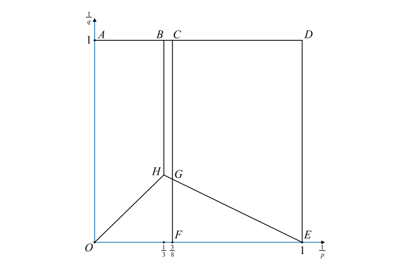
Figure 2. Interpolation diagram of $\mathcal{R}_{\delta}$

Theorem 4.1.

In the $(1/p,1/q)$-interpolation diagram (see Figure 2), let $O$ be the origin, and

$$A=\left(0,1\right),\quad B=\left(\frac{1}{3},1\right),\quad C=\left(\frac{3}{8},1\right),\quad D=\left(1,1\right),$$

$$E=\left(1,0\right),\quad F=\left(\frac{3}{8},0\right),\quad G=\left(\frac{3}{8},\frac{5}{16}\right),\quad H=\left(\frac{1}{3},\frac{1}{3}\right).$$

Then we have the following estimates. Here all line segments and polygons below include their boundaries, and the implicit constants are allowed to depend on $p,q$ but not $\delta$.

$$\begin{array}[]{|c|c|}\hline\cr R(p,q,\delta)&\forall(1/p,1/q)\in\\ \hline\cr\sim 1&OA\\ \hline\cr\begin{cases}\lesssim_{\varepsilon}\delta^{-\varepsilon}\\ \gtrsim(\log\delta^{-1})^{2/p}\end{cases}&OABH\backslash OA\\ \hline\cr\begin{cases}\lesssim_{\varepsilon}\delta^{-\varepsilon+\frac{1}{2}-\frac{3}{2p}}\\ \gtrsim\delta^{\frac{1}{2}-\frac{3}{2p}}\end{cases}&BCGH\backslash BH\\ \hline\cr\sim\delta^{\frac{1}{2}-\frac{3}{2p}}&CDEG\backslash CG\\ \hline\cr\sim\delta^{\frac{1}{q}-\frac{1}{p}}&EFG\backslash FG\\ \hline\cr\begin{cases}\lesssim_{\varepsilon}\delta^{-\varepsilon+\frac{1}{q}-\frac{1}{p}}\\ \gtrsim\delta^{\frac{1}{q}-\frac{1}{p}}\end{cases}&OFGH\backslash OF\\ \hline\cr\sim\delta^{-1/p}&OE\\ \hline\cr\end{array}$$

Proof.

We first come to the case $p=\infty$, namely, $(1/p,1/q)\in OA$. Here the upper bound is trivial, and the lower bound follows from taking $f=1_{B(0,1)}$.

For the case $q=\infty$, namely, $(1/p,1/q)\in OE$, the upper bound follows from interpolating between $p=1$ and $p=\infty$, and the lower bound follows from taking $f=1_{S}$ where

$$S=\{(x,af(x)):x\in[0,1],a\in[1,1+\delta]\}.$$ (4.1)

When $(1/p,1/q)\in OABH\backslash OA$, to prove the upper bound, by Hölder’s inequality, it suffices to prove the bound on $OH$ only. By [Zah12b], it holds at $H=(1/3,1/3)$. Then this follows from interpolating between $(0,0)$ and $(1/3,1/3)$. The lower bound follows from Theorem 1.3.

When $(1/p,1/q)\in CDEG\backslash CG$, the upper bound follows from [KW99]. The lower bound follows from taking $f=1_{T}$, where $T$ is a rectangle of dimensions $\delta^{1/2}\times\delta$.

When $(1/p,1/q)\in EFG\backslash FG$, the upper bound follows from interpolating between the points $(1/p,0)$ and $(\frac{1}{p},\frac{1}{2}-\frac{1}{2p})$. The lower bound follows from taking $f=1_{S}$, where $S$ is given by (4.1).

When $(1/p,1/q)\in BCGH\backslash BH$, the upper bound follows from interpolating between $BH$ and $CG$. The lower bound follows from taking $f=1_{T}$, where $T$ is a rectangle of dimensions $\delta^{1/2}\times\delta$.

When $(1/p,1/q)\in OFGH\backslash OF$, the upper bound follows from interpolating between $OF$ and the segments $OH,HG$. The lower bound follows from taking $f=1_{S}$, where $S$ is given by (4.1). ∎

4.1. Open problems

It is very natural to ask whether we can replace the $\varepsilon$-loss on the upper bounds of $R(p,q,\delta)$ to logarithmic loss (when we have a logarithmic lower bound), or to a constant loss (when we have a lower bound of the form $\delta^{\alpha}$, $\alpha>0$, without $\varepsilon$-loss). There are two key open problems to consider.

1. Improving the upper bound of $R(3,3,\delta)$. One may work through all the details of [Sch03] and [Wol00] to see if each time a loss of the form $\delta^{-\varepsilon}$ can be upgraded to just $\log\delta^{-1}$; if yes, then we can improve the bound to $(\log\delta^{-1})^{O(1)}$. However, improving to the lower bound $(\log\delta^{-1})^{2/p}$ proved in Theorem 1.3 seems to require a new method.

2. Removing the $\varepsilon$-loss in the range $\frac{1}{3}<\frac{1}{p}\leq\frac{3}{8}$. The condition $p<8/3$ is needed in the proof in the combinatorial argument in [KW99], but as far as the authors know, there are no counterexample showing why $p<8/3$ is necessary.

References

- [BR68] A. S. Besicovitch and R. Rado. A plane set of measure zero containing circumferences of every radius. J. London Math. Soc., 43:717–719, 1968.
- [CG24] M. Chen and S. Guo. The dichotomy of Nikodym sets and local smoothing estimates for wave equations. 2024. arXiv:2402.15476.
- [CGY23] M. Chen, S. Guo, and T. Yang. A multi-parameter cinematic curvature. 2023. arXiv:2306.01606.
- [CYZ23] X. Chen, L. Yan, and Y. Zhong. On the generalized Hausdorff dimension of Besicovitch sets. 2023. arXiv:2304.03633.
- [Dav72] R. O. Davies. Another thin set of circles. J. London Math. Soc. (2), 5:191–192, 1972.
- [HKLO23] S. Ham, H. Ko, S. Lee, and S. Oh. Remarks on dimension of unions of curves. Nonlinear Anal., 229:Paper No. 113207, 14, 2023.
- [Kin68] J. R. Kinney. A thin set of circles. The American Mathematical Monthly, 75(10):1077–1081, 1968.
- [KW99] L. Kolasa and T. Wolff. On some variants of the Kakeya problem. Pacific J. Math., 190(1):111–154, 1999.
- [PYZ22] M. Pramanik, T. Yang, and J. Zahl. A Furstenberg-type problem for circles, and a Kaufman-type restricted projection theorem in . 2022. arXiv:2207.02259.
- [Sch03] W. Schlag. On continuum incidence problems related to harmonic analysis. J. Funct. Anal., 201(2):480–521, 2003.
- [Sog91] C. D. Sogge. Propagation of singularities and maximal functions in the plane. Invent. Math., 104(2):349–376, 1991.
- [Tal80] M. Talagrand. Sur la mesure de la projection d’un compact et certaines familles de cercles. Bull. Sci. Math. (2), 104(3):225–231, 1980.
- [Wol97] T. Wolff. A Kakeya-type problem for circles. Amer. J. Math., 119(5):985–1026, 1997.
- [Wol00] T. Wolff. Local smoothing type estimates on for large . Geom. Funct. Anal., 10(5):1237–1288, 2000.
- [Zah12a] J. Zahl. estimates for an algebraic variable coefficient Wolff circular maximal function. Rev. Mat. Iberoam., 28(4):1061–1090, 2012.
- [Zah12b] J. Zahl. On the Wolff circular maximal function. Illinois J. Math., 56(4):1281–1295, 2012.
- [Zah23] J. Zahl. On maximal functions associated to families of curves in the plane. 2023. arXiv:2307.05894.