Magnon-squeezing-enhanced weak magnetic field sensing in cavity-magnon system

Abstract

Quantum noise and thermal noise are the two primary sources of noise that limit the sensitivity of weak magnetic field sensing. Although quantum noise has been widely addressed, effectively reducing thermal noise remains challenging in detecting weak magnetic fields. We employ an anisotropic elliptical YIG sphere as a magnetic field probe to establish a parametric amplification interaction of magnons and induce magnon squeezing effects. These effects can effectively suppress thermal noise in the magnon mode and amplify weak magnetic field signals from external sources. Specifically, complete suppression of thermal noise can be achieved by placing the YIG sphere in a squeezed vacuum reservoir. Our scheme has the potential to inspire advancements in thermal noise suppression for quantum sensing.

• May 2023

1 Introduction

In quantum sensing, [1, 2, 3, 4, 5, 6, 7, 8, 9, 10, 11, 12, 13, 14, 15, 16], the performance of the system is inevitably affected by quantum noise arising from quantum fluctuations and thermal noise resulting from system thermal fluctuations [17, 18, 19]. Thus, mitigating system noise and amplifying weak signals is crucial for improved sensing performance. Recently, sensing weak magnetic fields has been extensively explored using the cavity-magnon system [20, 21, 22, 23, 24, 25]. This system offers high-frequency tunability [26], high spin density [27], and a long coherence time in the magnon mode of yttrium iron garnet (YIG) spheres [28, 29]. Additionally, the ground state magnon mode (Kittel mode) of YIG spheres [30] can interact with various frequency bands of fields, including optical and microwave fields, making them excellent readout devices for detecting magnon modes [31, 32, 33, 34, 35, 36, 10]. Moreover, magnons can couple with superconducting qubits, providing advantages for spin readout [37, 38, 39]. Furthermore, the coupling of magnon-phonon-spin has been achieved [40], leading to groundbreaking applications in quantum information processing. These applications include the generation of non-classical magnon states [41, 42, 43, 44], Floquet engineering [45], magnon-driven nonreciprocal transport [46, 47, 48, 49, 50], and advancements in non-Hermitian quantum physics [51, 52, 53, 54].

The sensitivity of a cavity magnon system used for weak magnetic field sensing is primarily influenced by the microwave cavity’s quantum noise and the thermal noise of the YIG sphere’s magnon mode [10, 55]. Quantum noise comprises photons’ shot noise in the microwave cavity and the backaction noise resulting from the interaction between photons and magnons. The competition between these two types of noise creates the standard quantum limit (SQL) [56] and numerous methods, such as coherent quantum noise cancellation [57, 58, 59, 60], quadratic coupling [61, 62, 63], quantum squeezing [64, 65, 66], and Non-Markovian regime [67], have already been devised to surpass SQL by reducing the quantum noise in cavity optomechanical weak force and displacement sensing. Regarding thermal noise, one could naturally consider suppressing the thermal fluctuations by lowering the environment’s temperature, for example, using a dilution refrigerator [68]. However, achieving the desired low temperature in practical sensing scenarios could be challenging. In this regard, finding other mechanisms to reduce the impact of magnon thermal noise is significant.

This paper proposes a scheme to suppress thermal noise in magnetic field sensing. We leverage the unique anisotropic fluctuations of ellipsoidal YIG spheres in traditional cavity magnetic systems to induce a parameter-amplified magnon-magnon interaction. Through this magnon squeezing interaction, we can adjust the squeezing parameters, amplify the signal response of the magnon probe, and suppress additional noise in the microwave cavity of our weak magnetic field sensing system. This approach partially suppresses thermal noise and enhances the system’s sensitivity. Furthermore, immersion of the YIG sphere in a squeezed vacuum reservoir enables complete suppression of magnon mode thermal noise. The paper is structured as follows: Section 2 presents the model and Hamiltonian of the weak magnetic field sensing scheme with our anisotropic YIG spherical cavity magnon system. In Section 3, we delve into the system’s dynamics, provide an expression for the phase quadrature output of the weak magnetic field sensing system, and scrutinize the sensor’s performance. Section LABEL:IV employs the microwave-optical wave conversion homodyne detection method to analyze the system’s output spectrum, evaluating the response, additional noise, thermal noise, and sensitivity of weak magnetic sensing. Additionally, we offer a physical mechanism to elucidate the role of squeezed vacuum reservoirs and parametric interactions in thermal noise suppression. Finally, conclusions and discussions are presented in Section LABEL:V.

2 Weak sensing model and Hamiltonian

Figure 1: The schematic diagram of weak magnetic field sensing model. The system employs an anisotropic ellipsoidal YIG sphere as a probe to detect the external magnetic field. The microwave signal output from the cavity undergoes conversion into an optical signal via a microwave-optical wave conversion device (MOC). Subsequently, it traverses through a beam splitter (BS) before reaching two photodetectors (D1) and (D2). A subtractor is then utilized, followed by quadrature component spectrum detection, constituting a homodyne detection device. The external bias magnetic field $\rm B_{b}$ aligns with the z-axis, whereas the measured magnetic field $\rm B_{ex}(t)$ aligns with the x-direction. The amplitudes of the externally driven microwave field and the externally driven YIG spherical magnon mode are denoted as $\rm E_{l}$ and $\rm E_{b}$, respectively.

The system depicted in Fig. 1 consists of an anisotropic ellipsoidal YIG sphere within a microwave cavity. Two classical pump fields drive the microwave cavity and the YIG sphere, respectively, while an external magnetic field is applied along the x-axis. At the macroscopic spin limit, the Hamiltonian of the system can be expressed using the Holstein-Primakoff transformations as [69, 70, 71]

$$\hat{H} = \hbar\omega_{a}\hat{a}^{\dagger}\hat{a}+\hbar\omega_{0}\hat{m}^{\dagger}\hat{m}+\frac{\hbar\omega_{m}}{2}\left(\hat{m}^{2}+\hat{m}^{\dagger 2}\right)$$ (1)

$$+\hbar g_{0}(t)\left(\hat{m}+\hat{m}^{\dagger}\right)\left(\hat{a}+\hat{a}^{\dagger}\right)+i\hbar E_{l}(\hat{a}^{\dagger}e^{-i\omega_{l}t}-\hat{a}e^{i\omega_{l}t})$$

$$-\hbar\lambda B_{ex}(t)(\hat{m}+\hat{m}^{\dagger}),$$

Whereas the first two terms represent the free components of the microwave cavity field and the YIG spherical magnon mode, $\omega_{a}$ and $\omega_{0}$ denote the intrinsic frequencies of the cavity field and magnon, respectively. The operators $a$ and $m$ $(a^{\dagger},m^{\dagger})$ correspond to the annihilation (creation) operators of microwave photons and magnons. The frequency $\omega_{0}$ can be modulated by a bias magnetic field $B_{b}$ along the z-axis, with the gyromagnetic ratio $\gamma=2\pi\times{28}~{}\mathrm{GHz/T}$ [23]. The third term describes the parametric amplification interaction due to the anisotropy of an ellipsoidal YIG sphere, where $\omega_{m}=\gamma B_{b}-\omega_{0}$ stands for the corresponding anisotropic coupling coefficient, as elucidated in Refs. [70, 72]. The fourth term accounts for the dipole-dipole interaction between microwave photons and magnons. In contrast, the fifth and sixth terms denote the Hamiltonian driven by the two semi-classical pump fields. Here, $E_{l}=\sqrt{2P_{l}\kappa_{a}/\hbar\omega_{l}}$ represents the amplitude of the pump field with frequency $\omega_{l}$, where $P_{l}$ denotes the power of the microwave pump field, with $\kappa_{a}$ denoting the dissipation of the microwave cavity field. Notably, the coupling strength between photons and magnons adopts time-dependent coherent modulation, i.e., $g_{0}(t)=g_{0}+2g_{0}A\cos(\omega^{\prime}t)$, where $\omega^{\prime}$ and $A$ signify the coherent modulation frequency and amplitude, achievable through a Josephson parametric amplifier (JPA) to control the strength of magnon-photon coupling. Specifically, by adjusting the magnetic flux bias of the superconducting quantum interference device (SQUID) circuit in JPA, the inductance of SQUID can be modulated [10]. Here, $g_{0}=\gamma B_{0}\sqrt{5N}/2$ represents the cavity magnetic coupling coefficient without time-dependent modulation, and the intensity of the microwave field is denoted by $B_{0}$. The last term of the Hamiltonian represents the interaction between the measured magnetic field $B_{ex}(t)$ along the x-axis and the YIG sphere, with $\lambda=\gamma\sqrt{5N}/2$ being the corresponding interaction coefficient of external detected field-magnon.

To account for the influence of the parametric amplification interaction of magnons on the system, we diagonalize $H_{1}=\hbar\omega_{0}\hat{m}^{\dagger}\hat{m}+\frac{\hbar\omega_{m}}{2}\left(\hat{m}^{2}+\hat{m}^{\dagger 2}\right)$ through the squeezing transformation $\hat{m}=\cosh r_{m}\hat{M}+\sinh r_{m}\hat{M}^{\dagger}$, where $r_{m}=\frac{1}{4}\ln{\frac{\omega_{0}+\omega_{m}}{\omega_{0}-\omega_{m}}}$ denotes the degree of squeezing amplitude. Consequently, the Hamiltonian, after the squeezing transformation, takes the form

$$\hat{H^{s}} = \hbar\omega_{a}\hat{a}^{\dagger}\hat{a}+\hbar\omega^{\prime}_{0}\hat{M}^{\dagger}\hat{M}+\hbar g^{\prime}_{0}\left(\hat{M}+\hat{M}^{\dagger}\right)\left(\hat{a}+\hat{a}^{\dagger}\right)$$ (2)

$$+i\hbar E_{l}(\hat{a}^{\dagger}e^{-i\omega_{l}t}-\hat{a}e^{i\omega_{l}t})+i\hbar E_{b}(\hat{M}^{\dagger}e^{-i\omega_{b}t}-\hat{M}e^{i\omega_{b}t})$$

$$-\hbar\lambda B^{\prime}_{ex}(t)(\hat{M}+\hat{M}^{\dagger}),$$

where $\omega^{\prime}_{0}=\omega_{0}/\cosh(2r_{m})$ represents the corrected magnon frequency, $g_{0}^{\prime}(t)=g_{0}(t)e^{r_{m}}$, and $B^{\prime}_{ex}(t)=B_{ex}(t)e^{r_{m}}$ denote the enhanced cavity photon-magnon interaction intensity and the enhanced external magnetic field, respectively, and $\omega_{b}$ and $E_{b}$ represent the frequency and amplitude of the driving field of the magnon. Due to the external adjustable parameters $\omega^{\prime}$, $\omega_{l}$, and $\omega_{b}$, we set $\omega^{\prime}$ = $\omega_{l}+\omega_{b}$ and consider the rotational wave approximation. Consequently, after rotating with the semi-classical driving field frequencies $\omega_{L}$ and $\omega_{d}$, the Hamiltonian reads

$$\hat{H^{\prime}} =\hbar\Delta_{a}\hat{a}^{\dagger}\hat{a}+\hbar\Delta^{\prime}_{0}\hat{M}^{\dagger}\hat{M}+\hbar g^{\prime}\left(\hat{M}+\hat{M}^{\dagger}\right)\left(\hat{a}+\hat{a}^{\dagger}\right)$$

$$+i\hbar E_{l}(\hat{a}^{\dagger}-\hat{a})+i\hbar E_{b}(\hat{M}^{\dagger}-\hat{M})$$

$$-\hbar\lambda B^{\prime}_{ex}(t)(\hat{M}e^{-i\omega_{b}t}+\hat{M}^{\dagger}e^{i\omega_{b}t}),$$ (3)

where $\Delta_{a}=\omega_{a}-\omega_{l}$, $g^{\prime}=Ag_{0}e^{r_{m}}=ge^{r_{m}}$, and $\Delta^{\prime}_{0}=\omega^{\prime}_{0}-\omega_{b}$ represent the detuning between the cavity field and the driving microwave field, the effective cavity magnetic coupling strength, and the detuning of the magnon relative to the magnon driving field, respectively. Notably, to meet the rotational wave approximation, we require $g\ll\omega^{\prime}$, which can be satisfied by controlling the modulation amplitude $A$.

3 Dynamics of weak magnetic sensing system

In this section, we delve into our proposed scheme’s fluctuation and dissipation dynamics. Referring to the Hamiltonian in Eq. (2) from the preceding section, we derive the quantum Heisenberg-Langevin equation for the system [73, 74]

$$\dot{\hat{a}} = -i\Delta_{a}\hat{a}-\frac{\kappa_{a}}{2}\hat{a}-ig^{\prime}(\hat{M}+\hat{M}^{\dagger})+E_{l}+\sqrt{\kappa_{a}}\hat{a}_{\rm in}(t),$$

$$\dot{\hat{M}} = -i\Delta^{\prime}_{0}\hat{M}-\frac{\kappa_{m}}{2}\hat{M}-ig^{\prime}(\hat{a}+\hat{a}^{\dagger})+E_{b}+\sqrt{\kappa_{m}}\hat{M}_{\rm in}(t)$$ (4)

$$+i\lambda B^{\prime}_{ex}(t)e^{i\omega_{b}t},$$

Here, $\kappa_{m}$ denotes the dissipation rate of the YIG sphere, and $\hat{a}_{\rm in}(t)$, $\hat{M}_{\rm in}(t)=\cosh r_{m}\hat{m}_{\rm in}-\sinh r_{m}\hat{m}_{\rm in}^{\dagger}$ represent the vacuum input operator of the cavity field and the squeezed input noise operator of the magnon, respectively. The correlation functions for the input operators are given by

$$\left\langle\hat{a}_{\rm in}(t)\hat{a}_{\rm in}^{\dagger}\left(t^{\prime}\right)\right\rangle=(\bar{n}_{a}+1)\delta\left(t-t^{\prime}\right),$$

$$\left\langle\hat{m}_{\rm in}(t)\hat{m}_{\rm in}^{\dagger}\left(t^{\prime}\right)\right\rangle=(\bar{n}_{m}+1)\delta\left(t-t^{\prime}\right),$$ (5)

where $\bar{n}_{a}(\bar{n}_{m})=[\exp(\hbar\omega_{a}(\omega_{0})/k_{B}T)-1]^{-1}$ represents the average number of photons (magnons) in a thermal equilibrium state [41]. The modified squeezing input operator satisfies

$$\left\langle\hat{M}_{\rm in}(t)\hat{M}_{\rm in}^{\dagger}\left(t^{\prime}\right)\right\rangle=[\cosh(2r_{m})\bar{n}_{m}+\sinh^{2}(r_{m})+1]\delta\left(t-t^{\prime}\right),$$

$$\left\langle\hat{M}_{\rm in}^{\dagger}(t)\hat{M}_{\rm in}^{\dagger}\left(t^{\prime}\right)\right\rangle=-\sinh(2r_{m})(\bar{n}_{m}+1/2)\delta\left(t-t^{\prime}\right).$$ (6)

Since we consider a strong driving field, we can write the operator as the steady-state part plus the first-order fluctuations, i.e., $\hat{a}(M)=\bar{a}(\bar{m})+\delta{\hat{a}}(\delta{\hat{M}})$. Thus the Heisenberg- Langevin’s equation can be rewritten as

$$\delta\dot{\hat{a}} = -i\Delta_{a}\delta\hat{a}-\frac{\kappa_{a}}{2}\delta\hat{a}-ig^{\prime}(\delta\hat{M}+\delta\hat{M}^{\dagger})+\sqrt{\kappa_{a}}\hat{a}_{\rm in}(t),$$

$$\delta\dot{\hat{M}} = -i\Delta^{\prime}_{0}\delta\hat{M}-\frac{\kappa_{m}}{2}\delta\hat{M}-ig^{\prime}(\delta\hat{a}+\delta\hat{a}^{\dagger})+\sqrt{\kappa_{m}}\hat{M}_{\rm in}(t)$$ (7)

$$+i\lambda B^{\prime}_{ex}(t)e^{i\omega_{b}t}.$$

Considering the detection of the external magnetic field signal through the output of the microwave cavity field, we introduce the quadrature components $\delta\hat{X}_{a}=(\hat{a}^{\dagger}+\hat{a})/\sqrt{2}$, $\delta\hat{P}_{a}=(\hat{a}-\hat{a}^{\dagger})/\sqrt{2}i$, $\delta\hat{X}_{M}=(\hat{a}+\hat{a}^{\dagger})/\sqrt{2}i$, $\delta\hat{P}_{M}=(\hat{a}-\hat{a}^{\dagger})/\sqrt{2}i$. The Langevin equations for these quadrature components are

$$\delta\dot{\hat{X}}_{M} = \Delta^{\prime}_{0}\delta\hat{P}_{M}-\frac{\kappa_{m}}{2}\delta\hat{X}_{M}+\sqrt{\kappa_{m}}\hat{X}_{M}^{\prime\rm{in}},$$

$$\delta\dot{\hat{P}}_{M} = -\Delta^{\prime}_{0}\delta\hat{X}_{M}-2g^{\prime}\delta\hat{X}_{a}-\frac{\kappa_{m}}{2}\delta\hat{P}_{M}+\sqrt{\kappa_{m}}\hat{P}_{M}^{\rm{\prime in}},$$

$$\delta\dot{\hat{X}}_{a} = \Delta_{a}\delta\hat{P}_{a}-\frac{\kappa_{a}}{2}\delta\hat{X}_{a}+\sqrt{\kappa_{a}}\hat{X}_{a}^{\rm{in}},$$

$$\delta\dot{\hat{P}}_{a} = -\Delta_{a}\delta\hat{X}_{a}-2g^{\prime}\delta\hat{X}_{M}-\frac{\kappa_{a}}{2}\delta\hat{P}_{a}+\sqrt{\kappa_{a}}\hat{P}_{a}^{\rm{in}},$$ (8)

where $\hat{X}_{a}^{in}=(\hat{a}_{in}^{\dagger}+\hat{a}_{in})/\sqrt{2}$, $\hat{P}_{a}^{in}=(\hat{a}_{in}-\hat{a}_{in}^{\dagger})/\sqrt{2}i$, $\hat{X}_{M}^{\prime\rm in}=(\hat{M}_{in}^{\dagger}+\hat{M}_{in})/\sqrt{2}-\sqrt{2/\kappa_{m}}\lambda B^{\prime}_{ex}(t)\sin(\omega_{b}t)=\hat{X}_{M}^{\rm in}-\sqrt{2/\kappa_{m}}\lambda B^{\prime}_{ex}(t)\sin(\omega_{b}t)$, $\hat{P}_{M}^{\prime\rm in}=(\hat{M}_{in}-\hat{M}_{in}^{\dagger})/\sqrt{2}i+\sqrt{2/\kappa_{m}}\lambda B^{\prime}_{ex}(t)\cos(\omega_{b}t)=\hat{P}_{M}^{\rm in}+\sqrt{2/\kappa_{m}}\lambda B^{\prime}_{ex}(t)\cos(\omega_{b}t)$ are the quadratures of the cavity field and magnon mode correction noise input operators.

According to Eqs. (3), we can find that the correlation functions for the quadratures of the magnon mode are

$$\left\langle\hat{X}_{M}^{\rm in}(t)\hat{X}_{M}^{\rm in}\left(t^{\prime}\right)\right\rangle=e^{-2r_{m}}(\bar{n}_{m}+1/2)\delta\left(t-t^{\prime}\right),$$

$$\left\langle\hat{P}_{M}^{\rm in}(t)\hat{P}_{M}^{\rm in}\left(t^{\prime}\right)\right\rangle=e^{2r_{m}}(\bar{n}_{m}+1/2)\delta\left(t-t^{\prime}\right),$$ (9)

detailed derivation can be found in A. Eqs. (3) indicates that the magnon mode correlation function is modified to squeeze the amplitude quadrature fluctuations and increase the phase quadrature fluctuations. Therefore, we need to measure the cavity field phase quadrature to detect weak magnetic fields sensitively. Eqs. (3) indicate that the magnon mode correlation function is modified to squeeze the amplitude quadrature fluctuations and increase the phase quadrature fluctuations. Therefore, measuring the cavity field’s phase quadrature is crucial for sensitively detecting weak magnetic fields. To address the impact of noise on the system, we transform Eqs. (3) into the frequency domain space using the Fourier transform ${\hat{O}(\omega)=\int_{-\infty}^{\infty}dtO(t)e^{i\omega t}}$. Utilizing the input-output relationship for the phase quadrature component $\delta\hat{P}^{\rm out}_{a}=\sqrt{\kappa_{a}}\delta\hat{P}_{a}-\hat{P}^{\rm in}_{a}$, we obtain an expression for the phase quadrature of the cavity field as

$$\delta\hat{P}^{\rm{out}}_{a}(\omega) = K_{1}(\omega)\hat{X}^{\prime\rm{in}}_{m}(\omega)+K_{2}(\omega)\hat{P}^{\prime\rm{in}}_{m}(\omega)+K_{3}(\omega)\hat{X}^{\rm{in}}_{a}(\omega)$$ (10)

$$+K_{4}(\omega)\hat{P}^{\rm{in}}_{a}(\omega),$$

where

$${K_{1}}(\omega)= \frac{8g^{\prime}\sqrt{\kappa_{a}\kappa_{m}}\left(\kappa_{a}-2i\omega\right)\left(\kappa_{m}-2i\omega\right)}{64\Delta^{\prime}_{0}\Delta_{a}g^{\prime 2}+\left[\left(\kappa_{m}-2i\omega\right)^{2}+4\Delta^{\prime 2}_{0}\right]\left(4\omega^{2}+\kappa^{2}_{a}-4\Delta^{2}_{a}\right)},$$

$${K_{2}}(\omega)= \frac{16g^{\prime}\Delta^{\prime}_{0}\sqrt{\kappa_{a}\kappa_{m}}\left(\kappa_{a}-2i\omega\right)}{64\Delta^{\prime}_{0}\Delta_{a}g^{\prime 2}+\left[\left(\kappa_{m}-2i\omega\right)^{2}+4\Delta^{\prime 2}_{0}\right]\left(4\omega^{2}+\kappa^{2}_{a}-4\Delta^{2}_{a}\right)},$$

$${K_{3}}(\omega)= \frac{4\kappa_{a}\left[-16g^{\prime 2}\Delta^{\prime}_{0}+\Delta_{a}[(\kappa_{m}-2i\omega)^{2}+4\Delta^{\prime 2}_{0}]\right]}{64\Delta^{\prime}_{0}\Delta_{a}g^{\prime 2}+\left[\left(\kappa_{m}-2i\omega\right)^{2}+4\Delta^{\prime 2}_{0}\right]\left(4\omega^{2}+\kappa^{2}_{a}-4\Delta^{2}_{a}\right)},$$

$${K_{4}}(\omega)= -1-\frac{2\kappa_{a}\left(\kappa_{a}-2i\omega\right)\left[\left(\kappa_{m}-2i\omega\right)^{2}+4\Delta^{\prime 2}_{0}\right]}{64\Delta^{\prime}_{0}\Delta_{a}g^{\prime 2}+\left[\left(\kappa_{m}-2i\omega\right)^{2}+4\Delta^{\prime 2}_{0}\right]\left(4\omega^{2}+\kappa^{2}_{a}-4\Delta^{2}_{a}\right)},$$ (11)

with $\hat{X}^{\prime\rm{in}}_{M}(\omega)=\hat{X}^{\rm{in}}_{M}(\omega)+\lambda\sqrt{\frac{1}{2\kappa_{m}}}{i}\left[B^{\prime}_{ex}(\omega+\omega_{b})-B^{\prime}_{ex}(\omega-\omega_{b})\right]$ and $\hat{P}^{\prime\mathrm{in}}_{M}(\omega)=\hat{p}^{\rm{in}}_{M}(\omega)+\lambda\sqrt{\frac{1}{2\kappa_{m}}}\left[B^{\prime}_{ex}(\omega+\omega_{b})+B^{\prime}_{ex}(\omega-\omega_{b})\right]$ representing the modified quadrature component of the magnon in the frequency domain.

4 Weak magnetic field sensing using output spectrum analysis

4.1 The Role of Magnon squeezing in Anisotropic YIG Sphere

Direct homodyne detection of microwave photons remains impractical due to the experimental, developmental stage of the technology. As an alternative, microwave-to-optical frequency conversion technology offers a feasible approach by transferring photons from the microwave to the optical frequency band [75, 76, 77, 78, 79]. This initial conversion step bypasses the challenges associated with direct homodyne detection of microwave photons. Subsequent optical homodyne detection, applied to the converted optical frequency photons, is considered experimentally viable. It’s essential to clarify that our discussion does not delve into the specifics of conversion efficiency but emphasizes the broader implications of our proposed solution on sensing performance. Furthermore, leveraging homodyne detection, one can calculate the output spectrum of a weak magnetic field sensing system [80] as

$$S_{{\mathrm{out}}}(\omega)=\frac{1}{4\pi}\int d\omega^{\prime}e^{i(\omega+\omega^{\prime})t}\left[C_{P}(\omega,\omega^{\prime})+C_{P}(\omega^{\prime},\omega)\right]$$ (12)

with $C_{P}(\omega,\omega^{\prime})=\langle\delta\hat{P}^{\rm{out}}_{a}(\omega)\delta\hat{P}^{\rm{out}}_{a}(\omega^{\prime}\rangle$. For the current system, we have

$$S_{{\rm{out}}}(\omega) =(\bar{n}_{a}+\frac{1}{2})[|{K_{3}}(\omega)|^{2}+|{K_{4}}(\omega)|^{2}]$$

$$+|{K_{1}}(\omega)|^{2}[(\bar{n}_{m}+\frac{1}{2})/\xi+S^{\prime}_{B_{ex1}}]$$

$$+|{K_{2}}(\omega)|^{2}[(\bar{n}_{m}+\frac{1}{2})\xi+S^{\prime}_{B_{ex2}}],$$ (13)

Where $S^{\prime}_{B_{ex1}}=\xi S_{B_{ex1}}$ and $S^{\prime}_{B_{ex2}}=\xi S_{B_{ex2}}$ are the amplified signal spectral densities of the external magnetic field corresponding to the two channels of magnon amplitude quadrature component and a phase quadrature component, respectively, with $\xi=e^{2r_{m}}$ being the coefficient of amplification, from the output spectrum $S_{{\rm{out}}}(\omega)$, it can be seen that the second and third terms correspond to the squeezing effect and the anti-squeezing effect of the noise, respectively. In the squeezing effect, thermal noise can be reduced, while in the anti-squeezing effect, thermal noise is amplified. Therefore, to suppress the thermal noise of the system, a prerequisite is to make $|{K_{2}}(\omega)|^{2}=0$ so that the thermal noise only retains the squeezing effect, which can be attained by adjusting the detuning as $\Delta_{a}=\Delta^{\prime}_{0}=0$. Thus, one can obtain an output spectrum as

$$S_{{\rm{out}}}(\omega) =\frac{2\bar{n}_{a}+1}{2}|{K_{4}}(\omega)|^{2}+|{K_{1}}(\omega)|^{2}[\frac{2\bar{n}_{m}+1}{2\xi}+S^{\prime}_{B_{ex1}}].$$ (14)

Eq. (14) indicates that not only the thermal fluctuations of the magnon are exponentially suppressed, but also the backaction noise of the cavity field is eliminated. This can be further understood by rewriting the Langevin equations as

$$\delta\dot{\hat{X}}_{M} = -\frac{\kappa_{m}}{2}\delta\hat{X}_{M}+\sqrt{\kappa_{m}}\hat{X}_{M}^{\prime\rm{in}},$$

$$\delta\dot{\hat{P}}_{M} = -2g^{\prime}\delta\hat{X}_{a}-\frac{\kappa_{m}}{2}\delta\hat{P}_{M}+\sqrt{\kappa_{m}}\hat{P}_{M}^{\rm{\prime in}},$$

$$\delta\dot{\hat{X}}_{a} = -\frac{\kappa_{a}}{2}\delta\hat{X}_{a}+\sqrt{\kappa_{a}}\hat{X}_{a}^{\rm{in}},$$

$$\delta\dot{\hat{P}}_{a} = -2g^{\prime}\delta\hat{X}_{M}-\frac{\kappa_{a}}{2}\delta\hat{P}_{a}+\sqrt{\kappa_{a}}\hat{P}_{a}^{\rm{in}}.$$ (15)

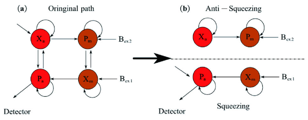
Figure 2: The schematic diagram of signal/noise transmission path. (a) The original path. (b) the path after implementing backaction avoidance and magnon squeezing.

It can be found that in the quadrature equations of the magnon mode (see the first two equations in Eqs. (4.1)), the amplitude quadrature and the phase quadrature are independent of each other. That is, the amplitude quadrature and the phase quadrature component can be measured independently simultaneously, and the phase quadrature component of the cavity field is only related to the amplitude quadrature. Therefore, our phase quadrature output spectrum will avoid the backaction noise caused by the cavity-magnon coupling effect. This is evident from the transition shown in Fig. 2, from panel (a) to panel (b). The phase quadrature component of the cavity field we aim to detect is separated into a squeezing path, enabling us to achieve low-noise sensing. On the contrary, the noise on the anti-squeezing path is amplified and captured by amplitude quadrature.

To better understand the noise suppression, one can express the output spectrum as

$$S_{{\rm{out}}}(\omega)=A_{m}(\omega)[N_{mth}(\omega)+N_{\rm{qn}}(\omega)+S_{B_{ex1}}],$$ (16)

where $A_{m}(\omega)$, $N_{\rm{qn}}(\omega)$, and $N_{mth}(\omega)$ represent the system’s response, additional noise, and magnon thermal noise, respectively. These are explicitly defined as

$$A_{m}(\omega)=\xi|{K_{1}}(\omega)|^{2},$$ (17)

$$N_{\rm{\rm{qn}}}(\omega)=\frac{(\bar{n}_{a}+\frac{1}{2})}{\xi}\frac{|{K_{4}}(\omega)|^{2}}{|{K_{1}}(\omega)|^{2}},$$ (18)

$$N_{mth}(\omega)=\frac{(\bar{n}_{m}+\frac{1}{2})}{\xi^{2}}.$$ (19)

From Eq. (17, 18, 19), we can surprisingly find that due to the squeezing effect, the response of the system to the external magnetic field can be amplified, which is conducive to more significant sensing of extremely weak magnetic field signals. Moreover, the system’s additional noise and the magnon’s thermal noise are also reduced, and the thermal noise decays faster.

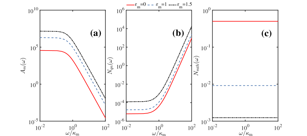
Figure 3: (a) The response $A_{\rm m}(\omega)$ of a weak magnetic field sensing system versus the normalized frequency $\omega/\kappa_{m}$ under different squeezing parameters. (b) Additional noise $N_{\rm qn}(\omega)$ versus the normalized frequency $\omega/\kappa_{m}$ under different squeezing parameters. (c) Thermal noise versus the normalized frequency $\omega/\kappa_{m}$ under different squeezing parameters. Here, the initial environmental temperature is $50~{}\rm{mK}$. It is worth noting that the legends for Fig. (a), (b), and Fig. (c) are consistent.

To elucidate the effects of various mechanisms on noise suppression, we conduct numerical simulations on several sensing performance indicators at low temperatures ($50\,\rm mK$), employing the experimental parameters cited in [21, 70, 10]: $\omega_{0}/2\pi=\omega_{a}/2\pi=37.5\,\rm{GHz}$, $\lambda/2\pi=14\times\sqrt{17.5}\,\rm{THz}$, $g/2\pi=2.5\,\rm{GHz}$, $\kappa_{m}/2\pi=15\,\rm{MHz}$, and $\kappa_{a}/2\pi=16.5\,\rm{MHz}$. Fig. 2(a) illustrates the response of the weak magnetic field sensing system. As the squeezing parameters increase, the signal amplification effect strengthens, attributed to the parametric amplification interaction of magnons acting as a parametric amplifier, thereby enhancing the external signal. Figs. 3(b) and 3(c) depict the suppression effect of magnon squeezing on additional noise and thermal noise, respectively. With increasing squeezing parameters, thermal and additional noise decrease by approximately three orders of magnitude. This reduction is straightforwardly understood as magnon squeezing significantly reduces vacuum fluctuations, leading to observable thermal noise decay. Additionally, the effective amplification of the signal through magnon squeezing results in a noticeable reduction of additional noise. This phenomenon is clearly illustrated in the comparison between Fig. 3(a) and 3(b). Furthermore, to evaluate the impact of cavity field dissipation on the sensing performance of the system, we plotted the variation curves of response, additional noise, and thermal noise at different cavity field dissipation rates, as illustrated in Fig. 4. The results indicate that increased cavity field dissipation adversely affects both the response and additional noise metrics (Fig. 5(a), (b)). This is because dissipation heightens the quantum noise within the cavity field, diminishing its ability to respond to the original signal accurately. Conversely, thermal noise remains unaffected by changes in cavity field dissipation, as depicted in Fig. 5(c). This is because thermal noise, having been normalized, is essentially background noise influenced solely by squeezing parameters.

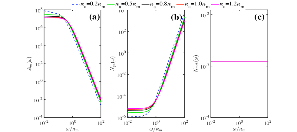
Figure 4: (a) The response $A_{\rm m}(\omega)$ of a weak magnetic field sensing system versus the normalized frequency $\omega/\kappa_{m}$ under different cavity field dissipation. (b) Additional noise $N_{\rm qn}(\omega)$ versus the normalized frequency $\omega/\kappa_{m}$ under different cavity field dissipation. (c) Thermal noise versus the normalized frequency $\omega/\kappa_{m}$ under different cavity field dissipation. The initial environmental temperature is $50~{}\rm{mK}$, squeezing parameter $r_{m}=1.5$. It is worth noting that the legends for Fig. (a), (b), and Fig. (c) are consistent.

Another parameter that significantly influences the response and additional noise is the cavity-magnon coupling strength, as depicted in Fig. 5(a) and Fig. 5(b). As the coupling strength increases, the response is enhanced, resulting in an amplified signal of the external magnetic field and a corresponding suppression of additional noise. This phenomenon can be explained from a physical perspective; with an increase in the cavity magnetic coupling strength, the energy exchange between the cavity photon-major systems becomes more efficient, facilitating the extraction of information regarding the external magnetic field.

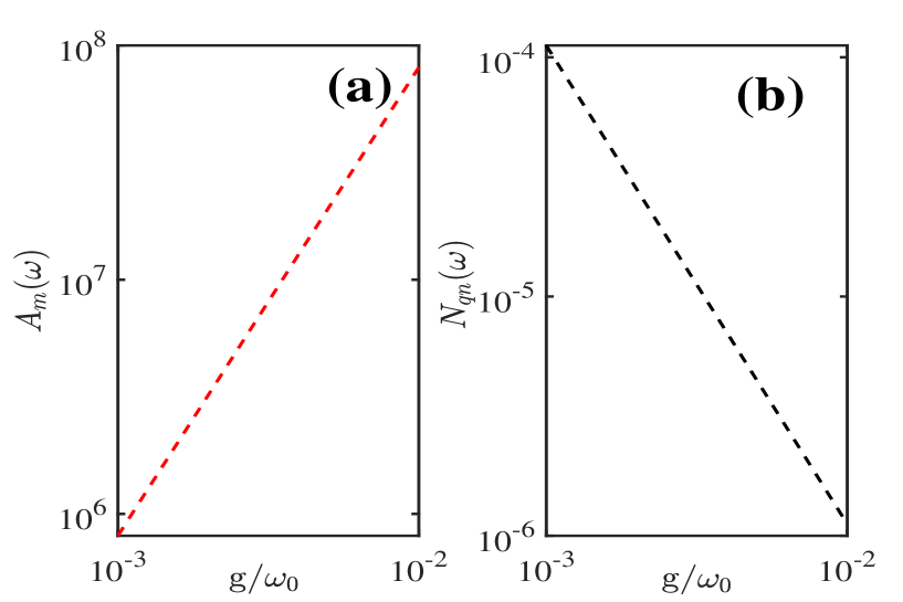
Figure 5: (a) The response $A_{\rm m}(\omega)$ of a weak magnetic field sensing system versus the normalized frequency $\omega/\kappa_{m}$ under different cavity- magnon coupling strengths. (b) Additional noise $N_{\rm qn}(\omega)$ versus the normalized frequency $\omega/\kappa_{m}$ under different cavity-magnon coupling strengths. Here, the initial environmental temperature is $50~{}\rm{mK}$,squeezing parameter $r_{m}=1.5$, $\kappa_{a}$=0.2$\kappa_{m}$.

To perform a detailed analysis of the system’s sensitivity, we consider the total noise spectral density of the system. According to Eq. (10), the total noise amplitude can be expressed as

$$\hat{B}_{noise}(\omega)=\frac{\sqrt{2\kappa_{m}}}{\lambda{\xi}}\hat{X}^{\rm{in}}_{m}(\omega)+\frac{\sqrt{2\kappa_{m}}K_{4}(\omega)}{K_{1}(\omega)\lambda\sqrt{\xi}}\hat{P}^{\rm{in}}_{a}(\omega).$$ (20)

The total noise intensity can be quantified using the symmetric noise power spectral density. This measure is directly detectable by a quantum spectrum analyzer and is defined as follows [60]

$$S_{Bnoise}(\omega)\delta(\omega+\omega^{\prime})=\frac{1}{2}(\langle\hat{B}_{noise}(\omega)\hat{B}_{noise}(\omega^{\prime})\rangle+c.c.).$$ (21)

Thus, the total noise spectrum can be given as

$$S_{Bnoise}(\omega)=\frac{2\kappa_{m}}{\lambda^{2}}[N_{Mth}(\omega)+N_{\rm{ad}}(\omega)].$$ (22)

Next, we further discuss the system’s signal-to-noise ratio to define its sensitivity. Generally speaking, the signal-to-noise ratio is the ratio of the measured signal to noise. For our system, it can be written in the following form

$$B_{SNR}(\omega)=\frac{|{B_{ex}}(\omega)|}{\sqrt{S_{Bnoise}(\omega)}},$$ (23)

the numerator represents the signal of the external magnetic field to be measured, and the denominator represents the noise information. To find the minimum detectable signal, we set the signal-to-noise ratio to 1, which can provide the minimum detectable signal, i.e., $B_{dmin}=\sqrt{S_{Bnoise}(\omega)}$ can be given. Therefore, we define the minimum detectable signal as sensitivity [10, 80], which is defined as

$$Y_{sensitivity}(\omega) = \sqrt{S_{Bnoise}(\omega)}$$ (24)

$$= \frac{\sqrt{{2\kappa_{m}}[N_{Mth}(\omega)+N_{\rm{ad}}(\omega)]}}{\lambda}.$$

The sensitivity of the system depends on the additional noise and magnon thermal noise, the dissipation rate ($\kappa_{m}$) of the YIG sphere, and the coupling strength ($\lambda$) of the external magnetic field. A smaller $Y_{\text{sensitivity}}(\omega)$ value indicates higher sensitivity.

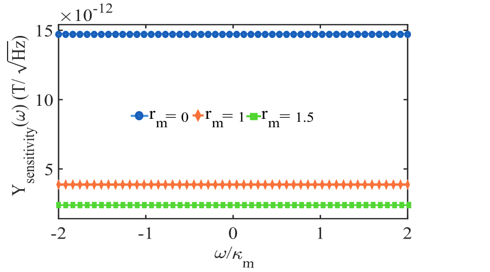
Figure 6: The sensitivity $Y_{\rm sensitivity}(\omega)$ of a weak magnetic field sensing system versus the normalized frequency $\omega/\kappa_{m}$ under different squeezing parameters. We set the initial environmental temperature to be $280~{}\rm{K}$.

In Fig. 6, we plot the sensitivity of the weak magnetic sensing system as a function of the normalized frequency $\omega/\kappa_{m}$ under different squeezing parameters. At room temperature, our sensitivity improves by one order of magnitude compared to without magnon squeezing. Furthermore, we observe that the sensitivity remains relatively constant with the normalized frequency, indicating that thermal noise predominantly influences the system. Nonetheless, our results demonstrate a significant enhancement over the scenario without squeezing.

4.2 The Role of Magnon squeezed Vacuum Reservoir

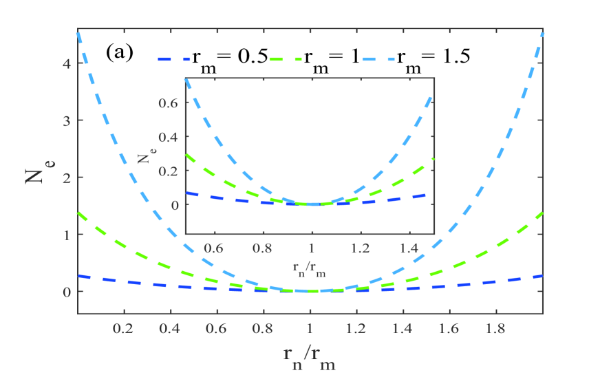
Figure 7: (a) The corrected effective average number of magnon $N_{e}$ versus the relative squeezing parameters $r_{\rm n}/r_{\rm m}$. (b) The corrected effective average number of magnon $N_{e}$ versus the squeezing phase $\Phi_{\rm n}/\pi$.

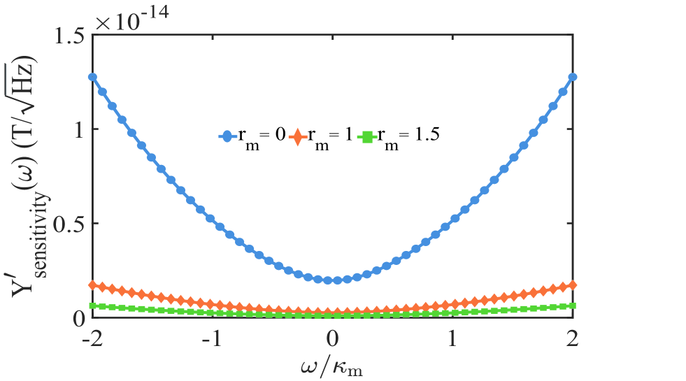
Figure 8: The sensitivity $Y^{\prime}_{\rm sensitivity}(\omega)$ versus the normalized frequency $\omega/\kappa_{m}$ under different squeezing parameters. We set the initial environmental temperature to be $280~{}\rm{K}$.

In this section, we demonstrate that introducing a specific magnon-squeezed vacuum reservoir for continued suppression of thermal noise can significantly enhance sensitive sensing performance. We introduce a magnon squeezing vacuum reservoir with a squeezing parameter $r_{n}$ and a phase $\Phi_{n}$. Consequently, the correlation function of the input noise operator of the magnon can be further modified as follows

$$\left\langle M^{c}_{in}(t)M_{in}^{{c}\dagger}\left(t^{\prime}\right)\right\rangle =\left(N_{e}+1\right)\delta\left(t-t^{\prime}\right),$$

$$\left\langle M_{in}^{{c}\dagger}(t)M_{in}^{{c}}\left(t^{\prime}\right)\right\rangle =N_{e}\delta\left(t-t^{\prime}\right),$$

$$\left\langle M_{in}^{{c}\dagger}(t)M_{in}^{{c}\dagger}\left(t^{\prime}\right)\right\rangle =M_{e}\delta\left(t-t^{\prime}\right),$$

$$\left\langle M_{in}^{{c}\dagger}(t)M_{in}^{{c}\dagger}\left(t^{\prime}\right)\right\rangle =M^{*}_{e}\delta\left(t-t^{\prime}\right).$$ (25)

where

$$N_{e}= \sinh^{2}\left(r_{n}\right)\cosh^{2}\left(r_{m}\right)+\sinh^{2}\left(r_{m}\right)\cosh^{2}\left(r_{n}\right)+$$

$$\frac{1}{2}\cos\left(\Phi_{n}\right)\sinh\left(2r_{n}\right)\sinh\left(2r_{m}\right),$$

$$M_{e}= {\left[\cosh\left(r_{n}\right)\sinh\left(r_{m}\right)+e^{i\Phi_{n}}\sinh\left(r_{n}\right)\cosh\left(r_{m}\right)\right]\times}$$

$${\left[\cosh\left(r_{n}\right)\cosh\left(r_{m}\right)+e^{-i\Phi_{n}}\sinh\left(r_{n}\right)\sinh\left(r_{m}\right)\right],}$$ (26)

represent the corrected effective average number of magnons and the interaction coefficient of two magnons, respectively [81]. In Fig. 7, we plot the curve of $N_{\rm e}$ as a function of the squeezing parameter and phase of the vacuum reservoir. Notably, if $r_{n}=r_{m}$ and $\Phi=\pm\pi$, the effective number of magnons reduces to zero, leading to a simplified expression of sensitivity

$$Y^{\prime}_{sensitivity}(\omega)\approx\frac{\sqrt{{2\kappa_{m}}N_{\rm{ad}}(\omega)}}{\lambda}.$$ (27)

This implies complete suppression of magnon thermal noise, with sensitivity $Y^{\prime}_{\text{sensitivity}}$ solely dependent on the additional noise $N_{\rm{ad}}$ of the weak magnetic field sensing system, a component of the microwave cavity field. Furthermore, given the previous achievement of backaction evading, the sensing system’s noise is only part of the shot noise of the cavity field. To better highlight the significant advantage of combining the parametric amplification effect of squeezed vacuum reservoirs and magnons on sensitivity, as shown in Fig. 8, we plot the sensitivity with different squeezing parameters under complete suppression of magnon thermal noise. Surprisingly, with a squeezing parameter $r_{m}=1.5$, the sensitivity reaches the $\rm fT/\sqrt{\rm Hz}$ level at room temperature (280K). Therefore, our theoretical scheme can achieve ultra-high sensitivity weak magnetic field sensing.

5 DISCUSSION and CONCLUSIONS

In this paper, we achieved magnon squeezing interaction through an anisotropic YIG sphere. Additionally, squeezing may be induced by various methods such as utilizing squeezed vacuum fields [82], employing dual-tone microwave fields to stimulate magnon mode [83], or utilizing two microwave fields to drive qubits within a magnetic qubit system nested in a cavity [84]. Our study focuses on suppressing thermal noise in weak magnetic sensing within cavity magnon systems. We propose modifying the shape of the YIG sphere from spherical to ellipsoidal to achieve magnon squeezing and alter the correlation function of the quadrature components of the magnon mode, resulting in significant suppression of thermal noise. Furthermore, successfully coupling the YIG sphere magnon with a squeezed vacuum reservoir can enable perfect thermal noise suppression, allowing the system sensitivity to reach the order of fT even at room temperature. Our scheme provides a crucial foundation for improvement in weak magnetic field sensing. Magnons serve as excellent probes for external magnetic fields, and achieving low noise in microwave cavities and ultrastrong coupling of cavity photon-magnon facilitates converting the external magnetic field signal through magnons to photons, detectable by spectral analyzers. Moreover, in dark matter detection, the coupling between axions and standard model matter can generate a pseudo magnetic field detectable by magnons, with the extracted signal detectable by the optical readout, as initially proposed in [85]. The idea and experimentation of using cavity magnetic systems for weak magnetic field sensing have been continually evolving [86, 87, 88, 89], providing a promising platform for dark matter detection. Although experimentally realizing a squeezed vacuum reservoir for magnons remains challenging, there is relevant literature on preparing single-mode and dual-mode squeezed states of magnons [90, 91, 92, 93]. This can be achieved through other methods, such as reservoir engineering or optical lattice. Moving forward, we aim to investigate the impact of entanglement and other quantum resources on weak magnetic field sensing.

Appendix A Modified Magnon Correlation Functions

In this section, we derive the correlation function for the quadrature components of the magnon mode, as presented in Eqs. (3) in the main text.

For a magnon mode located in a thermal equilibrium reservoir, its input correlation function is expressed in the following form

$$\left\langle\hat{m}_{\rm in}(t)\hat{m}_{\rm in}^{\dagger}\left(t^{\prime}\right)\right\rangle = (\bar{n}_{m}+1)\delta\left(t-t^{\prime}\right),$$

$$\left\langle\hat{m}_{\rm in}^{\dagger}(t)\hat{m}_{\rm in}\left(t^{\prime}\right)\right\rangle = \bar{n}_{m}\delta\left(t-t^{\prime}\right),$$ (28)

In the main text, we introduce the correlation function satisfied by the input noise operator after squeezing transformation $\hat{m}=\cosh r_{m}\hat{M}+\sinh r_{m}\hat{M}^{\dagger}$ as follows

$$\left\langle\hat{M}_{\rm in}(t)\hat{M}_{\rm in}^{\dagger}\left(t^{\prime}\right)\right\rangle=[\cosh(2r_{m})\bar{n}_{m}+\sinh^{2}(r_{m})+1]\delta\left(t-t^{\prime}\right),$$

$$\left\langle\hat{M}_{\rm in}^{\dagger}(t)\hat{M}_{\rm in}^{\dagger}\left(t^{\prime}\right)\right\rangle=-\sinh(2r_{m})(\bar{n}_{m}+1/2)\delta\left(t-t^{\prime}\right),$$

$$\left\langle\hat{M}_{\rm in}(t)\hat{M}_{\rm in}\left(t^{\prime}\right)\right\rangle=-\sinh(2r_{m})(\bar{n}_{m}+1/2)\delta\left(t-t^{\prime}\right),$$

$$\left\langle\hat{M}_{\rm in}^{\dagger}(t)\hat{M}_{\rm in}\left(t^{\prime}\right)\right\rangle=[\cosh(2r_{m})\bar{n}_{m}+\sinh^{2}(r_{m})]\delta\left(t-t^{\prime}\right).$$ (29)

Next, we introduce the quadrature components of the amplitude and phase of the magnon mode, which are expressed as follows

$$\hat{X}_{M}^{\rm in} = (\hat{M}_{in}^{\dagger}+\hat{M}_{in})/\sqrt{2},$$

$$\hat{P}_{M}^{\rm in} = (\hat{M}_{in}-\hat{M}_{in}^{\dagger})/\sqrt{2}i.$$ (30)

Afterwards, we calculate the two relationships of Eqs. (3), The correlation functions for amplitude and phase quadrature components of magnon mode are

$$\left\langle\hat{X}_{M}^{\rm in}(t)\hat{X}_{M}^{\rm in}\left(t^{\prime}\right)\right\rangle =\frac{1}{2}\left[\left\langle\hat{M}_{\rm in}(t)\hat{M}_{\rm in}\left(t^{\prime}\right)\right\rangle+\left\langle\hat{M}_{\rm in}(t)\hat{M}_{\rm in}^{\dagger}\left(t^{\prime}\right)\right\rangle+\left\langle\hat{M}_{\rm in}^{\dagger}(t)\hat{M}_{\rm in}\left(t^{\prime}\right)\right\rangle+\left\langle\hat{M}_{\rm in}^{\dagger}(t)\hat{M}_{\rm in}^{\dagger}\left(t^{\prime}\right)\right\rangle\right]$$

$$=\frac{1}{2}\left[-2\sinh(2r_{m})(\bar{n}_{m}+1/2)+2\cosh(2r_{m})\bar{n}_{m}+2\sinh^{2}(r_{m})+1\right]$$

$$=\frac{1}{2}\left[-2\sinh(2r_{m})(\bar{n}_{m}+1/2)+2\cosh(2r_{m})\bar{n}_{m}+\cosh(2r_{m})\right]$$

$$=\frac{1}{2}\left[-2\sinh(2r_{m})(\bar{n}_{m}+1/2)+2\cosh(2r_{m})(\bar{n}_{m}+1/2)\right]$$

$$=e^{-2r_{m}}(\bar{n}_{m}+1/2)\delta\left(t-t^{\prime}\right).$$ (31)

$$\left\langle\hat{P}_{M}^{\rm in}(t)\hat{P}_{M}^{\rm in}\left(t^{\prime}\right)\right\rangle =-\frac{1}{2}\left[\left\langle\hat{M}_{\rm in}(t)\hat{M}_{\rm in}\left(t^{\prime}\right)\right\rangle-\left\langle\hat{M}_{\rm in}(t)\hat{M}_{\rm in}^{\dagger}\left(t^{\prime}\right)\right\rangle-\left\langle\hat{M}_{\rm in}^{\dagger}(t)\hat{M}_{\rm in}\left(t^{\prime}\right)\right\rangle+\left\langle\hat{M}_{\rm in}^{\dagger}(t)\hat{M}_{\rm in}^{\dagger}\left(t^{\prime}\right)\right\rangle\right]$$

$$=-\frac{1}{2}\left[-2\sinh(2r_{m})(\bar{n}_{m}+1/2)-2\cosh(2r_{m})\bar{n}_{m}-2\sinh^{2}(r_{m})-1\right]$$

$$=-\frac{1}{2}\left[-2\sinh(2r_{m})(\bar{n}_{m}+1/2)-2\cosh(2r_{m})\bar{n}_{m}-\cosh(2r_{m})\right]$$

$$=-\frac{1}{2}\left[-2\sinh(2r_{m})(\bar{n}_{m}+1/2)-2\cosh(2r_{m})(\bar{n}_{m}+1/2)\right]$$

$$=e^{2r_{m}}(\bar{n}_{m}+1/2)\delta\left(t-t^{\prime}\right).$$ (32)

So, we obtained Eqs. (3) in the main text.

Disclosures

The authors declare no conflicts of interest related to this article.

References

References

- [1] Degen C L, Reinhard F and Cappellaro P 2017 Rev. Mod. Phys. 89(3) 035002 URL https://link.aps.org/doi/10.1103/RevModPhys.89.035002
- [2] Forstner S, Prams S, Knittel J, van Ooijen E D, Swaim J D, Harris G I, Szorkovszky A, Bowen W P and Rubinsztein-Dunlop H 2012 Phys. Rev. Lett. 108(12) 120801 URL https://link.aps.org/doi/10.1103/PhysRevLett.108.120801
- [3] Takeuchi Y, Matsuzaki Y, Miyanishi K, Sugiyama T and Munro W J 2019 Phys. Rev. A 99(2) 022325 URL https://link.aps.org/doi/10.1103/PhysRevA.99.022325
- [4] Long X, He W T, Zhang N N, Tang K, Lin Z, Liu H, Nie X, Feng G, Li J, Xin T, Ai Q and Lu D 2022 Phys. Rev. Lett. 129(7) 070502 URL https://link.aps.org/doi/10.1103/PhysRevLett.129.070502
- [5] Kumar P, Biswas T, Feliz K, Kanamoto R, Chang M S, Jha A K and Bhattacharya M 2021 Phys. Rev. Lett. 127(11) 113601 URL https://link.aps.org/doi/10.1103/PhysRevLett.127.113601
- [6] Li B B, Bílek J, Hoff U B, Madsen L S, Forstner S, Prakash V, Schäfermeier C, Gehring T, Bowen W P and Andersen U L 2018 Optica 5 850–856 URL https://opg.optica.org/optica/abstract.cfm?URI=optica-5-7-850
- [7] Forstner S, Sheridan E, Knittel J, Humphreys C L, Brawley G A, Rubinsztein-Dunlop H and Bowen W P 2014 Advanced Materials 26 6348–6353 URL https://onlinelibrary.wiley.com/doi/abs/10.1002/adma.201401144
- [8] Barry J F, Irion R A, Steinecker M H, Freeman D K, Kedziora J J, Wilcox R G and Braje D A 2023 Phys. Rev. Appl. 19(4) 044044 URL https://link.aps.org/doi/10.1103/PhysRevApplied.19.044044
- [9] Cao Y and Yan P 2019 Phys. Rev. B 99(21) 214415 URL https://link.aps.org/doi/10.1103/PhysRevB.99.214415
- [10] Ebrahimi M S, Motazedifard A and Harouni M B 2021 Phys. Rev. A 103(6) 062605 URL https://link.aps.org/doi/10.1103/PhysRevA.103.062605
- [11] Xu A N and Liu Y C 2022 Phys. Rev. A 106(1) 013506 URL https://link.aps.org/doi/10.1103/PhysRevA.106.013506
- [12] Schliesser A, Anetsberger G, Rivière R, Arcizet O and Kippenberg T J 2008 New Journal of Physics 10 095015 URL https://dx.doi.org/10.1088/1367-2630/10/9/095015
- [13] Anetsberger G, Gavartin E, Arcizet O, Unterreithmeier Q P, Weig E M, Gorodetsky M L, Kotthaus J P and Kippenberg T J 2010 Phys. Rev. A 82(6) 061804 URL https://link.aps.org/doi/10.1103/PhysRevA.82.061804
- [14] Li B B, Bulla D, Prakash V, Forstner S, Dehghan-Manshadi A, Rubinsztein-Dunlop H, Foster S and Bowen W P 2018 APL Photonics 3 120806 ISSN 2378-0967 URL https://doi.org/10.1063/1.5055029
- [15] Colombano M F, Arregui G, Bonell F, Capuj N E, Chavez-Angel E, Pitanti A, Valenzuela S O, Sotomayor-Torres C M, Navarro-Urrios D and Costache M V 2020 Phys. Rev. Lett. 125(14) 147201 URL https://link.aps.org/doi/10.1103/PhysRevLett.125.147201
- [16] Chu P H, Kim Y J and Savukov I 2019 Phys. Rev. D 99(7) 075031 URL https://link.aps.org/doi/10.1103/PhysRevD.99.075031
- [17] Clerk A A, Devoret M H, Girvin S M, Marquardt F and Schoelkopf R J 2010 Rev. Mod. Phys. 82(2) 1155–1208 URL https://link.aps.org/doi/10.1103/RevModPhys.82.1155
- [18] Safavi-Naeini A H, Chan J, Hill J T, Gröblacher S, Miao H, Chen Y, Aspelmeyer M and Painter O 2013 New Journal of Physics 15 035007 URL https://dx.doi.org/10.1088/1367-2630/15/3/035007
- [19] Zhang W Z, Chen L B, Cheng J and Jiang Y F 2019 Phys. Rev. A 99(6) 063811 URL https://link.aps.org/doi/10.1103/PhysRevA.99.063811
- [20] Rao J, Wang C Y, Yao B, Chen Z J, Zhao K X and Lu W 2023 Phys. Rev. Lett. 131(10) 106702 URL https://link.aps.org/doi/10.1103/PhysRevLett.131.106702
- [21] Zhang X, Zou C L, Jiang L and Tang H X 2014 Phys. Rev. Lett. 113(15) 156401 URL https://link.aps.org/doi/10.1103/PhysRevLett.113.156401
- [22] Zare Rameshti B, Viola Kusminskiy S, Haigh J A, Usami K, Lachance-Quirion D, Nakamura Y, Hu C M, Tang H X, Bauer G E and Blanter Y M 2022 Physics Reports 979 1–61 ISSN 0370-1573 cavity Magnonics URL https://www.sciencedirect.com/science/article/pii/S0370157322002460
- [23] Zhang X, Zou C L, Jiang L and Tang H X 2016 Science Advances 2 e1501286 URL https://www.science.org/doi/abs/10.1126/sciadv.1501286
- [24] Hussain B, Qamar S and Irfan M 2022 Phys. Rev. A 105(6) 063704 URL https://link.aps.org/doi/10.1103/PhysRevA.105.063704
- [25] Zhang Q, Wang J, Lu T X, Huang R, Nori F and Jing H 2024 Science China Physics, Mechanics and Astronomy 67 100313 ISSN 1869-1927 URL https://doi.org/10.1007/s11433-024-2432-9
- [26] Sharma S, Blanter Y M and Bauer G E W 2017 Phys. Rev. B 96(9) 094412 URL https://link.aps.org/doi/10.1103/PhysRevB.96.094412
- [27] Cherepanov V, Kolokolov I and L’vov V 1993 Physics Reports 229 81–144 ISSN 0370-1573 URL https://www.sciencedirect.com/science/article/pii/037015739390107O
- [28] Goryachev M, Farr W G, Creedon D L, Fan Y, Kostylev M and Tobar M E 2014 Phys. Rev. Appl. 2(5) 054002 URL https://link.aps.org/doi/10.1103/PhysRevApplied.2.054002
- [29] Bourhill J, Kostylev N, Goryachev M, Creedon D L and Tobar M E 2016 Phys. Rev. B 93(14) 144420 URL https://link.aps.org/doi/10.1103/PhysRevB.93.144420
- [30] Kittel C 1948 Phys. Rev. 73(2) 155–161 URL https://link.aps.org/doi/10.1103/PhysRev.73.155
- [31] Soykal O O and Flatté M E 2010 Phys. Rev. Lett. 104(7) 077202 URL https://link.aps.org/doi/10.1103/PhysRevLett.104.077202
- [32] Haigh J A, Nunnenkamp A, Ramsay A J and Ferguson A J 2016 Phys. Rev. Lett. 117(13) 133602 URL https://link.aps.org/doi/10.1103/PhysRevLett.117.133602
- [33] Osada A, Hisatomi R, Noguchi A, Tabuchi Y, Yamazaki R, Usami K, Sadgrove M, Yalla R, Nomura M and Nakamura Y 2016 Phys. Rev. Lett. 116(22) 223601 URL https://link.aps.org/doi/10.1103/PhysRevLett.116.223601
- [34] Zhang X, Zhu N, Zou C L and Tang H X 2016 Phys. Rev. Lett. 117(12) 123605 URL https://link.aps.org/doi/10.1103/PhysRevLett.117.123605
- [35] Viola Kusminskiy S, Tang H X and Marquardt F 2016 Phys. Rev. A 94(3) 033821 URL https://link.aps.org/doi/10.1103/PhysRevA.94.033821
- [36] Fan Z Y, Shen R C, Wang Y P, Li J and You J Q 2022 Phys. Rev. A 105(3) 033507 URL https://link.aps.org/doi/10.1103/PhysRevA.105.033507
- [37] Ren Y l, Ma S l and Li F l 2022 Phys. Rev. A 106(5) 053714 URL https://link.aps.org/doi/10.1103/PhysRevA.106.053714
- [38] Wolski S P, Lachance-Quirion D, Tabuchi Y, Kono S, Noguchi A, Usami K and Nakamura Y 2020 Phys. Rev. Lett. 125(11) 117701 URL https://link.aps.org/doi/10.1103/PhysRevLett.125.117701
- [39] Xie J k, Ma S l and Li F l 2020 Phys. Rev. A 101(4) 042331 URL https://link.aps.org/doi/10.1103/PhysRevA.101.042331
- [40] Kim T, Leiner J C, Park K, Oh J, Sim H, Iida K, Kamazawa K and Park J G 2018 Phys. Rev. B 97(20) 201113 URL https://link.aps.org/doi/10.1103/PhysRevB.97.201113
- [41] Li J, Zhu S Y and Agarwal G S 2018 Phys. Rev. Lett. 121(20) 203601 URL https://link.aps.org/doi/10.1103/PhysRevLett.121.203601
- [42] Zhang Z, Scully M O and Agarwal G S 2019 Phys. Rev. Res. 1(2) 023021 URL https://link.aps.org/doi/10.1103/PhysRevResearch.1.023021
- [43] Yuan H Y, Yan P, Zheng S, He Q Y, Xia K and Yung M H 2020 Phys. Rev. Lett. 124(5) 053602 URL https://link.aps.org/doi/10.1103/PhysRevLett.124.053602
- [44] Sun F X, Zheng S S, Xiao Y, Gong Q, He Q and Xia K 2021 Phys. Rev. Lett. 127(8) 087203 URL https://link.aps.org/doi/10.1103/PhysRevLett.127.087203
- [45] Xu J, Zhong C, Han X, Jin D, Jiang L and Zhang X 2020 Phys. Rev. Lett. 125(23) 237201 URL https://link.aps.org/doi/10.1103/PhysRevLett.125.237201
- [46] Kong C, Xiong H and Wu Y 2019 Phys. Rev. Appl. 12(3) 034001 URL https://link.aps.org/doi/10.1103/PhysRevApplied.12.034001
- [47] Wang Y P, Rao J W, Yang Y, Xu P C, Gui Y S, Yao B M, You J Q and Hu C M 2019 Phys. Rev. Lett. 123(12) 127202 URL https://link.aps.org/doi/10.1103/PhysRevLett.123.127202
- [48] Zhu N, Han X, Zou C L, Xu M and Tang H X 2020 Phys. Rev. A 101(4) 043842 URL https://link.aps.org/doi/10.1103/PhysRevA.101.043842
- [49] Yu T, Zhang Y X, Sharma S, Zhang X, Blanter Y M and Bauer G E W 2020 Phys. Rev. Lett. 124(10) 107202 URL https://link.aps.org/doi/10.1103/PhysRevLett.124.107202
- [50] Ren Y l, Ma S l, Xie J k, Li X k, Cao M t and Li F l 2022 Phys. Rev. A 105(1) 013711 URL https://link.aps.org/doi/10.1103/PhysRevA.105.013711
- [51] Harder M, Yang Y, Yao B M, Yu C H, Rao J W, Gui Y S, Stamps R L and Hu C M 2018 Phys. Rev. Lett. 121(13) 137203 URL https://link.aps.org/doi/10.1103/PhysRevLett.121.137203
- [52] Xu P C, Rao J W, Gui Y S, Jin X and Hu C M 2019 Phys. Rev. B 100(9) 094415 URL https://link.aps.org/doi/10.1103/PhysRevB.100.094415
- [53] Yang Y, Wang Y P, Rao J W, Gui Y S, Yao B M, Lu W and Hu C M 2020 Phys. Rev. Lett. 125(14) 147202 URL https://link.aps.org/doi/10.1103/PhysRevLett.125.147202
- [54] Lu T X, Zhang H, Zhang Q and Jing H 2021 Phys. Rev. A 103(6) 063708 URL https://link.aps.org/doi/10.1103/PhysRevA.103.063708
- [55] Liu Z, Liu Y q, Mai Z y, Yang Y j, Zhou N n and Yu C s 2024 Phys. Rev. A 109(2) 023709 URL https://link.aps.org/doi/10.1103/PhysRevA.109.023709
- [56] Aspelmeyer M, Kippenberg T J and Marquardt F 2014 Rev. Mod. Phys. 86(4) 1391–1452 URL https://link.aps.org/doi/10.1103/RevModPhys.86.1391
- [57] Bariani F, Seok H, Singh S, Vengalattore M and Meystre P 2015 Phys. Rev. A 92(4) 043817 URL https://link.aps.org/doi/10.1103/PhysRevA.92.043817
- [58] Motazedifard A, Bemani F, Naderi M H, Roknizadeh R and Vitali D 2016 New Journal of Physics 18 073040 URL https://dx.doi.org/10.1088/1367-2630/18/7/073040
- [59] Allahverdi H, Motazedifard A, Dalafi A, Vitali D and Naderi M H 2022 Phys. Rev. A 106(2) 023107 URL https://link.aps.org/doi/10.1103/PhysRevA.106.023107
- [60] Wimmer M H, Steinmeyer D, Hammerer K and Heurs M 2014 Phys. Rev. A 89(5) 053836 URL https://link.aps.org/doi/10.1103/PhysRevA.89.053836
- [61] Sainadh U S and Kumar M A 2020 Phys. Rev. A 102(6) 063523 URL https://link.aps.org/doi/10.1103/PhysRevA.102.063523
- [62] Chao S L, Yang Z, Zhao C S, Peng R and Zhou L 2021 Opt. Lett. 46 3075–3078 URL https://opg.optica.org/ol/abstract.cfm?URI=ol-46-13-3075
- [63] Zhang S D, Wang J, Zhang Q, Jiao Y F, Zuo Y L, Şahin K Özdemir, Qiu C W, Nori F and Jing H 2024 Optica Quantum 2 222–229 URL https://opg.optica.org/opticaq/abstract.cfm?URI=opticaq-2-4-222
- [64] Xu X and Taylor J M 2014 Phys. Rev. A 90(4) 043848 URL https://link.aps.org/doi/10.1103/PhysRevA.90.043848
- [65] Zhao W, Zhang S D, Miranowicz A and Jing H 2019 Science China Physics, Mechanics and Astronomy 63 224211 ISSN 1869-1927 URL https://doi.org/10.1007/s11433-019-9451-3
- [66] Wang J, Zhang Q, Jiao Y F, Zhang S D, Lu T X, Li Z, Qiu C W and Jing H 2024 Applied Physics Reviews 11 031409 ISSN 1931-9401 (Preprint https://pubs.aip.org/aip/apr/article-pdf/doi/10.1063/5.0208107/20084417/031409_1_5.0208107.pdf) URL https://doi.org/10.1063/5.0208107
- [67] Zhang W Z, Han Y, Xiong B and Zhou L 2017 New J. Phys 19 083022 URL https://dx.doi.org/10.1088/1367-2630/aa68d9
- [68] Kuhn A G, Teissier J, Neuhaus L, Zerkani S, van Brackel E, Deléglise S, Briant T, Cohadon P F, Heidmann A, Michel C, Pinard L, Dolique V, Flaminio R, Taïbi R, Chartier C and Le Traon O 2014 Applied Physics Letters 104 044102 ISSN 0003-6951 URL https://doi.org/10.1063/1.4863666
- [69] Holstein T and Primakoff H 1940 Phys. Rev. 58(12) 1098–1113 URL https://link.aps.org/doi/10.1103/PhysRev.58.1098
- [70] Sharma S, Bittencourt V A S V, Karenowska A D and Kusminskiy S V 2021 Phys. Rev. B 103(10) L100403 URL https://link.aps.org/doi/10.1103/PhysRevB.103.L100403
- [71] Tiablikov S V 2013 Methods in the quantum theory of magnetism (Springer)
- [72] Yuan H, Cao Y, Kamra A, Duine R A and Yan P 2022 Physics Reports 965 1–74 ISSN 0370-1573 quantum magnonics: When magnon spintronics meets quantum information science URL https://www.sciencedirect.com/science/article/pii/S0370157322000977
- [73] Benguria R and Kac M 1981 Phys. Rev. Lett. 46(1) 1–4 URL https://link.aps.org/doi/10.1103/PhysRevLett.46.1
- [74] Gardiner C W and Collett M J 1985 Phys. Rev. A 31(6) 3761–3774 URL https://link.aps.org/doi/10.1103/PhysRevA.31.3761
- [75] Rueda A, Sedlmeir F, Collodo M C, Vogl U, Stiller B, Schunk G, Strekalov D V, Marquardt C, Fink J M, Painter O, Leuchs G and Schwefel H G L 2016 Optica 3 597–604 URL https://opg.optica.org/optica/abstract.cfm?URI=optica-3-6-597
- [76] Kim B, Kurokawa H, Sakai K, Koshino K, Kosaka H and Nomura M 2023 Phys. Rev. Appl. 20(4) 044037 URL https://link.aps.org/doi/10.1103/PhysRevApplied.20.044037
- [77] Xing F F, Qin L G, Tian L J, Wu X Y and Huang J H 2023 Opt. Express 31 7120–7133 URL https://opg.optica.org/oe/abstract.cfm?URI=oe-31-5-7120
- [78] Weaver M J, Duivestein P, Bernasconi A C, Scharmer S, Lemang M, Thiel T C v, Hijazi F, Hensen B, Gröblacher S and Stockill R 2023 Nature Nanotechnology ISSN 1748-3395 URL https://doi.org/10.1038/s41565-023-01515-y
- [79] Rochman J, Xie T, Bartholomew J G, Schwab K C and Faraon A 2023 Nature Communications 14 1153 ISSN 2041-1723 URL https://doi.org/10.1038/s41467-023-36799-0
- [80] Motazedifard A, Dalafi A, Bemani F and Naderi M H 2019 Phys. Rev. A 100(2) 023815 URL https://link.aps.org/doi/10.1103/PhysRevA.100.023815
- [81] Lü X Y, Wu Y, Johansson J R, Jing H, Zhang J and Nori F 2015 Phys. Rev. Lett. 114(9) 093602 URL https://link.aps.org/doi/10.1103/PhysRevLett.114.093602
- [82] Li J, Zhu S Y and Agarwal G S 2019 Phys. Rev. A 99(2) 021801 URL https://link.aps.org/doi/10.1103/PhysRevA.99.021801
- [83] Zhang W, Wang D Y, Bai C H, Wang T, Zhang S and Wang H F 2021 Opt. Express 29 11773–11783 URL https://opg.optica.org/oe/abstract.cfm?URI=oe-29-8-11773
- [84] Guo Q, Cheng J, Tan H and Li J 2023 Phys. Rev. A 108(6) 063703 URL https://link.aps.org/doi/10.1103/PhysRevA.108.063703
- [85] Barbieri R, Cerdonio M, Fiorentini G and Vitale S 1989 Physics Letters B 226 357–360 ISSN 0370-2693 URL https://www.sciencedirect.com/science/article/pii/0370269389912094
- [86] Crescini N, Alesini D, Braggio C, Carugno G, D’Agostino D, Di Gioacchino D, Falferi P, Gambardella U, Gatti C, Iannone G, Ligi C, Lombardi A, Ortolan A, Pengo R, Ruoso G and Taffarello L (QUAX Collaboration) 2020 Phys. Rev. Lett. 124(17) 171801 URL https://link.aps.org/doi/10.1103/PhysRevLett.124.171801
- [87] Flower G, Bourhill J, Goryachev M and Tobar M E 2019 Physics of the Dark Universe 25 100306 ISSN 2212-6864 URL https://www.sciencedirect.com/science/article/pii/S2212686418301985
- [88] Ruoso G, Lombardi A, Ortolan A, Pengo R, Braggio C, Carugno G, Gallo C S and Speake C C 2016 Journal of Physics: Conference Series 718 042051 URL https://dx.doi.org/10.1088/1742-6596/718/4/042051
- [89] Barbieri R, Braggio C, Carugno G, Gallo C, Lombardi A, Ortolan A, Pengo R, Ruoso G and Speake C 2017 Physics of the Dark Universe 15 135–141 ISSN 2212-6864 URL https://www.sciencedirect.com/science/article/pii/S2212686417300031
- [90] Qian H, Zuo X, Fan Z Y, Cheng J and Li J 2024 Phys. Rev. A 109(1) 013704 URL https://link.aps.org/doi/10.1103/PhysRevA.109.013704
- [91] Zhao X D, Zhao X, Jing H, Zhou L and Zhang W 2013 Phys. Rev. A 87(5) 053627 URL https://link.aps.org/doi/10.1103/PhysRevA.87.053627
- [92] Wuhrer D, Rohling N and Belzig W 2022 Phys. Rev. B 105(5) 054406 URL https://link.aps.org/doi/10.1103/PhysRevB.105.054406
- [93] Wuhrer D, Rózsa L, Nowak U and Belzig W 2023 Phys. Rev. Res. 5(4) 043124 URL https://link.aps.org/doi/10.1103/PhysRevResearch.5.043124