Efficient simulation of the SABR model
Abstract
We propose an efficient and reliable simulation scheme for the stochastic-alpha-beta-rho (SABR) model. The two challenges of the SABR simulation lie in sampling (i) the integrated variance conditional on terminal volatility and (ii) the terminal price conditional on terminal volatility and integrated variance. For the first sampling procedure, we analytically derive the first four moments of the conditional average variance, and sample it from the moment-matched shifted lognormal approximation. For the second sampling procedure, we approximate the conditional terminal price as a constant-elasticity-of-variance (CEV) distribution. Our CEV approximation preserves the martingale condition and precludes arbitrage, which is a key advantage over Islah’s approximation used in most SABR simulation schemes in the literature. Then, we adopt the exact sampling method of the CEV distribution based on the shifted-Poisson-mixture Gamma random variable. Our enhanced procedures avoid the tedious Laplace inversion algorithm for sampling integrated variance and non-efficient inverse transform sampling of the forward price in some of the earlier simulation schemes. Numerical results demonstrate our simulation scheme to be highly efficient, accurate, and reliable.
keywords:
SABR model, Monte Carlo simulation, constant elasticity of variance process, shifted-Poisson-mixture gamma distribution1 Introduction
The stochastic-alpha-beta-rho (SABR) model proposed by Hagan et al. (2002) has been widely adopted in option pricing due to its ability to capture volatility smile or skew using a few parameters, and exhibiting consistency in revealing the dynamic behavior between price and smile. On one hand, it is common in equity options that the implied volatility of out-of-money options are generally higher than that of the in-the-money counterparts, known as the volatility skew. On the other hand, the relatively symmetric volatility smile is common in the foreign exchange options. The SABR model can capture the volatility skew and volatility smile in the respective markets. In addition, the SABR model exhibits consistency in the dynamic behavior of volatility smile or skew, where an increase of the price of the underlying asset leads to shifting of the volatility smile or skew to a higher price (Hagan et al., 2002). The SABR model can generate such co-movements correctly while the local volatility model fails to do so (Derman and Kani, 1998; Dupire, 1997).
In their original paper, Hagan et al. (2002) derived an analytic implied volatility formula under the SABR model via an asymptotic expansion in small time-to-maturity. It has been a standard practice for practitioners to obtain the option price from the implied volatility using the Black–Scholes formula. However, Hagan et al. (2002)’s approximation becomes unreliable under large time-to-maturity or when the option is deep-out-of-the-money. As a result, one important stream of the SABR model research has been improving the implied volatility approximation (Obłój, 2007; Paulot, 2015; Lorig et al., 2017; Gulisashvili et al., 2018; Yang et al., 2017; Choi and Wu, 2021a). Notably, Antonov and Spector (2012) obtained a more accurate approximation by mapping the implied volatilities under the correlated cases to those of the uncorrelated cases, under which more analytic properties of the SABR model become available.
Another stream of research, to which this paper belongs, is developing efficient simulation algorithms of the SABR model. With growing popularity of the SABR model, there has been demand for pricing path-dependent derivatives using the model. Since analytic expansion approaches are limited to pricing the European options, the Monte Carlo method becomes a natural choice. In particular, the research on the SABR simulation has been stimulated by less than perfect performance of the Euler and Milstein time-discretization schemes. Since the SABR model imposes an absorbing boundary condition at the origin, the time discretization scheme should be more carefully implemented; naive truncation at the origin leads to large deviation from the original SABR model. Typically, it is necessary to use a small time discretization step to decrease the discretization errors due to its low order of convergence, thus suffering from heavy computation load.
Several simulation algorithms (Chen et al., 2012; Cai et al., 2017; Leitao et al., 2017a, b; Cui et al., 2018; Grzelak et al., 2019; Kyriakou et al., 2023) have been proposed for efficient simulation of the SABR model. Simulating the SABR process over a relatively large time step requires sequentially sampling terminal volatility, average variance, and terminal price at the next simulation time point. Since the last two sampling procedures are challenging, existing methods are differentiated with reference to different choices of the algorithms for these two steps. These earlier simulation algorithms have achieved some success in that they overcome the issue of the time-discretization method. However, there are still many gaps to be filled in order to make SABR simulation more efficient.
Regarding the average variance conditional on the terminal volatility, Chen et al. (2012) sampled the quantity through the mean-and-variance matched lognormal (LN) variable. While the sampling procedures are fast, the time step cannot be large since the derived mean and variance are valid in small-time limit only. For more accurate sampling, researchers used various version of the transform of the average variance. Leitao et al. (2017a, b) derived the approximate Fourier transform of the unconditional average variance recursively, while Cai et al. (2017) adopted the analytically available Laplace transform of the reciprocal of the conditional average variance (Matsumoto and Yor, 2005). However, these approaches are cumbersome and time-consuming due to the tedious numerical inverse transform for constructing the cumulative distribution function (CDF) and iterative root-finding for inverse transform sampling. Cui et al. (2021) approximated the volatility dynamics with the continuous-time Markov chain (CTMC) over volatility grids. Their approach is also not immune from heavy computation and complicated implementation. Kyriakou et al. (2023) used moment-matched Pearson family of distributions for efficient sampling. For such purpose, they rely on numerical evaluation of the four moments from the conditional Laplace transform.
Sampling the terminal price conditional on the terminal variance and average variance is perhaps more challenging. Unlike the other stochastic volatility models that are based on the geometric Brownian motion (BM), the constant-elasticity-of-variance (CEV) feature of the SABR model does not admit an analytically tractable form of the conditional price distribution. As a result, the distribution has to be approximated by an analytic form first even before the corresponding sampling algorithm is considered. For the approximation of the conditional price distribution, almost all existing algorithms (Chen et al., 2012; Cai et al., 2017; Leitao et al., 2017a, b; Cui et al., 2018; Grzelak et al., 2019; Kyriakou et al., 2023) adopted Islah (2009)’s noncentral chi-squared (NCX2) distribution approximation unquestionably. However, the failure of the martingale property in this approximation has not been critically examined among these papers. Leitao et al. (2017a, b) applied an ad-hoc correction on the simulation prices to enforce the martingale property. Therefore, the possibility of better approximation of the conditional price distribution that preserves the martingale should be explored.
The lack of fast sampling algorithm for the approximated distribution is the last hurdle in constructing an efficient SABR simulation algorithm. The inverse transform sampling with numerical root-finding is accurate but tediously slow. The mean-and-variance-match quadratic Gaussian sampling has been adopted in Chen et al. (2012), Leitao et al. (2017a, b), and Cui et al. (2021) to speed up sampling. However, it is limited to small time step due to the nature of approximation. Also, it cannot be used efficiently when the price is close to zero due to the absorbing boundary condition.
This paper proposes an accurate, efficient, and reliable SABR simulation algorithm, filling the gaps in all steps of the simulation procedure. The contributions of this paper are three-fold. Firstly, we derive the first four conditional moments of the conditional average variance analytically. We then use the shifted lognormal (SLN) distribution matching the moments for fast sampling of the average variance. As we use the moments that are higher in order and exact for any arbitrary time step, the validity of our algorithm can be extended to larger time step. Secondly, we present an alternative approximation of the conditional price distribution based on the CEV process. Our approximation is superior to the widely adopted Islah (2009)’s approximation because it preserves the martingale property by construction. Lastly, we employ the algorithms of Makarov and Glew (2010) and Kang (2014) that are capable of sampling the CEV price process for an arbitrary time step. Their algorithms are fast since the CEV price can be expressed by a compound random variable composed of three elementary (i.e., gamma-Poison-gamma) random variables.
This paper is organized as follows. Section 2 presents the formulation of the SABR model and reviews some of its analytic properties. Section 3 describes our SLN approximation for sampling the average variance. In Section 4, we present the CEV distribution approximation of the conditional forward price, and an exact sampling algorithm for the CEV distribution via the shifted Poisson-mixture Gamma distribution. In Sections 3 and 4, our simulation algorithm is compared to those in the existing literature. In particular, we argue that the CEV distribution is a better alternative to the widely adopted Islah (2009)’s approximation as it preserves the martingale condition. Section 5 presents our comprehensive numerical experiments that serve to assess accuracy, efficiency and reliability of different simulation schemes and analytic approximation methods, focusing on the more challenging choices of parameters, such as large time-to-maturity. Conclusive remarks are summarized in Section 6.
2 Formulation of the SABR model and its special cases
In this section, we introduce the SABR model and review some of its analytic properties. The two steps of the SABR simulation are outlined. Specifically, we discuss some special cases where the SABR simulation becomes straightforward.
2.1 SABR model
The governing stochastic differential equations (SDE) for the SABR volatility model (Hagan et al., 2002) are given by
| (1) |
where and are the stochastic processes for the forward price and volatility, respectively, is the vol-of-vol, is the elasticity of variance parameter, and and are the standard BMs that are correlated with correlation coefficient . We also define two variables for later use:
2.2 Average variance, conditional expectation, and two-step simulation procedures
Regarding the simulation step, without loss of generality, we sample the volatility and forward price at time (i.e., and ) for some time step given time . Accordingly, the filtration up to time (e.g., and ) is implicitly assumed.
Since the volatility process in Eq. (1) follows a geometric BM, , simulating from time to can be easily done by observing
| (2) |
Here, is the standard deviation of over the time step . This quantity is used as a measure of small-time limit.
Like the simulation schemes of other SV models, integrated variance conditional on initial and terminal volatility values plays an important role in the SABR model simulation. Given the initial and terminal volatility (i.e., and ), we define the conditional average variance between and as
| (3) |
Here, we normalize the integral by in order that becomes a dimensionless quantity in the order of one. Specifically, converges to one in the limit of . From the simulation step in Eq. (2), is equivalently conditioned by as
For notational simplicity, we omit the dependence on or and simply write .
Almost all SABR simulation algorithms are required to perform the following two steps, given the filtration up to , to sufficient accuracy:
- Step 1
-
: simulation of the average variance conditional on (or ),
- Step 2
-
: simulation of the forward price conditional on and .
As both simulation steps pose challenges, the previous studies on the topic have proposed numerous algorithms for the two steps. This paper also aims to innovate the two steps, details are presented in Sections 3 and 4, respectively.
Regarding Step 2, let us also define the conditional expectation of :
| (4) |
which is essential for the discussion of the simulation algorithms of Step 2. We also omit the dependence on and , and simply write .
2.3 Special cases
Before introducing our simulation algorithm, we review several special cases of the SABR model. In these cases, Step 2 is relatively easier while Step 1 remains challenging. Reviewing these cases also helps building intuitions for our new algorithm.
Normal () SABR model: When , conditional on and , integrating from to reveals that the terminal forward price follows the normal distribution with mean and variance :
where the conditional expectation is given by
| (5) |
Therefore, Step 2 becomes trivial as long as can be sampled accurately in Step 1. Choi et al. (2019) have also found an exact closed-form expression for sampling without separating Steps 1 and 2. Moreover, note that , as well as can be negative in this special case as the origin is not a boundary. The normal SABR model is different from the limit of the SABR model, where the origin is an absorbing boundary. In the view of the above, the SABR model under is not a concern of our study.
Lognormal () SABR model: When , conditional on and , integrating from to yields that the terminal forward price follows the LN distribution with mean and log variance :
| (6) |
where is a standard normal variate independent of and . The conditional expectation is given by
| (7) |
Therefore, Step 2 becomes trivial as well when .
This special case provides an important observation, which derives an intuition for our CEV approximation when (to be discussed Section 4).
Remark 1.
The joint distribution of and satisfies
for any initial volatility .
Proof.
It follows from the law of total expectation:
Zero vol-of-vol () SABR model: When , the SABR model is visualized as the stochastic volatility version of the CEV model:
| (8) |
with the absorbing boundary condition at the origin.
Definition 1.
We define the distribution of resulting from the CEV dynamics in Eq. (8) as the CEV distribution,
parameterized by the elasticity-of-variance parameter , mean 111If , then regardless of the values of and ., and variance . The probability distribution function (PDF) and CDF of the CEV distribution will be shown later in Proposition 5.
Therefore, in the zero vol-of-vol () limit, from the SABR model (unconditionally) follows . Step 2 is reduced to sampling from the CEV distribution. However, this is not a trivial task as we discuss later in Section 4.
Uncorrelated () SABR model: The terminal forward price also exhibits a CEV distribution under non-zero vol-of-vol () and zero correlation () case, albeit conditionally. Conditional on , the terminal price follows the CEV distribution:
Basically, plays the role of stochastic time clock of the CEV model. As in the case, Step 2 is reduced to sampling from the CEV distribution in this case. Unlike the case, is conditioned by only since conditional expectation is always without depending on . Thus, should be understood as the unconditional average variance in this context. Therefore, the European option price can be simplified to one dimensional integral of the CEV option price over the (unconditional) distribution of . Choi and Wu (2021b) have approximated the integral using the Gaussian quadrature together with the LN distribution fitted to the (unconditional) mean and variance of .
Completing the discussion on the four special cases, we are left with the most general case with and , under which the conditional distribution of is not analytically tractable. One has to resort to an approximation. The approximation should be reduced to the special cases discussed above under various continuous limits.
3 First simulation step: Sampling average variance
This section presents our simulation method for sampling . We also compare with other most popular simulation methods, highlighting the computational advantages of our simulation scheme.
3.1 Sampling from the moment-matched SLN approximation
We sample from the SLN distribution matched to the first three moments of .
Definition 2 (SLN variable).
The SLN random variable, , is given by
where is a standard normal variate. Here, is the mean of , and are the weight and variance of the LN component, respectively. When , is reduced to the LN variable with mean and log variance .
The mean, coefficient of variation, skewness, and ex-kurtosis of are given by
where .
Remark 2.
While the skewness and ex-kurtosis of distribution follow the conventional definitions, the coefficient of variation is defined as the ratio of standard deviation to mean:
The coefficient of variation is an important dimensionless quantity that characterizes non-negative distributions such as the LN or SLN distributions.
Proposition 1 (SLN distribution matched to the first three moments).
Given mean , coefficient of variance , and skewness , the parameters of the SLN distribution matching , , and are analytically given by
Proof.
We first fit to the given skewness :
Substituting transforms the equation to a special case of the cubic equation:
where the unique positive root is analytically given by 222See https://en.wikipedia.org/wiki/Cubic_equation#Hyperbolic_solution_for_one_real_root.
The expression for follows from . Next, we fit to the given coefficient of variance :
Remark 3.
For an LN random variable (i.e., ), is determined by matching the coefficient of variation :
Chen et al. (2012) has sampled through the LN random variable fitted to the mean and variance of in the small-time limit.
Next, we derive the first four conditional moments of , whose analytic formulas are presented in the next proposition.
Proposition 2 (Conditional moments of average variance).
Given and , the first four raw moments of (i.e., and ) are obtained as below.
where the conditioning variable, and , are exchangeable by , and the coefficients, and , are the functions of them:
and and are the PDF and CDF of the standard normal distribution, respectively.
Proof.
Remark 4.
Remark 5.
From the first four raw moments, the coefficient of variation , skewness , and ex-kurtosis of are obtained as
where is the variance.
From Propositions 1 and 2, it is possible to sample from the SLN variable whose parameters are fitted to the first three moments of exactly. However, we take a simpler computational approach that uses a fixed obtained from the small-time limit. It is shown to be effective as well.
Proposition 3 (SLN in the small-time limit).
Proof.
In A, the coefficient of variation and skewness of are expanded around as
Using Taylor’s expansion, we have
so that the shift parameter converges to
Once is determined, we fit to match the coefficient of variation:
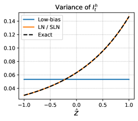
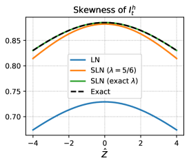
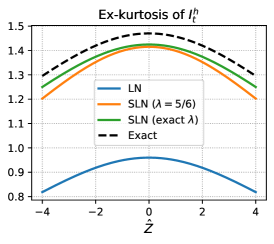
As we demonstrate in the numerical results shown in Figure 1, this approximation is highly reliable not only for small but also for . ∎
3.2 Comparison to other simulation methods in literature
Our sampling method for is much faster and easier to implement compared to other methods in the literature, such as Chen et al. (2012), Cai et al. (2017), Leitao et al. (2017a, b) and Cui et al. (2021).
Our method is considered as an extension of Chen et al. (2012) as they use an LN approximation matched to mean and variance of . However, they derive the mean and variance only in the small-time limit, so the time step should be small accordingly. We enhance the method by deriving the moments analytically and matching to higher moments with the SLN approximation. Figure 1 displays the accuracy of variance, skewness, and ex-kurtosis of obtained from our SLN approximation. The left figure shows that Chen et al. (2012)’s small-time approximation of the variance is not accurate across the dependency while our approximation is exact. The middle figure shows that the SLN approximation gives the correct skewness value as the parameters are fitted up to skewness. Moreover, the skewness under the simple SLN scheme with also agrees well for . Even though the two SLN schemes do not use the ex-kurtosis in the parameter calibration, the ex-kurtosis is close to the true value, justifying our choice of the SLN random variable.
Cai et al. (2017) computed the analytic form of the Laplace transform of the CDF of the reciprocal of the average variance 1/, then used the Euler inversion formula to obtain the CDF of 1/. After obtaining the CDF, they used the inverse transform method, which requires some tedious root-finding procedures such as Newton’s method or bisection method to sample .
Leitao et al. (2017a, b) used recursion schemes to find the characteristic function of the logarithm of and then employed the inverse Fourier technique COS method (Fang and Oosterlee, 2008) to recover its PDF. They then computed the Pearson correlation coefficient of and , then the bivariate copula distribution based on the CDF of and approximate CDF of . Finally, they adopted the direct inverse transform method based on linear interpolation to sample .
Cui et al. (2021) used the continuous-time Markov chain (CTMC) to approximate the space of the volatility process with finite number of states. In their procedure, they first fixed the volatility grids, computed the transition probability density at these grids based on the exponential of the generator matrix and used the inverse transform method to sample the volatility. After obtaining the volatility values, they computed the conditional characteristic function of the integrated variance, again based on the exponential of the generator matrix. They then adopted the Fourier sampler to get the CDF of the integrated variance, which first computed the PDF of the integrated variance via the orthogonal projection. Finally, they simulated the integrated variance using the closed-form inverse function.
Putting aside the issue of accuracy of the simulation methods of , these simulation methods invariably include some tedious and time-consuming procedures such as the adoption of the inverse Laplace/Fourier transform calculation, root-finding steps in the inverse transform methods or computation of the exponential of matrices. However, our SLN simulation methods for exhibits easy and fast implementation. As shown in the numerical experiments reported in Section 5, our simulation methods for demonstrate significant savings in computational time and high level of accuracy.
4 Second simulation step: Sampling forward price
This section presents our CEV approximation for and its sampling method.
4.1 CEV approximation of the conditional price
Proposition 4 proposes our approximation of for the general case. Our choice of the approximation is a very natural and intuitive extension of the special cases discussed in Section. 2.3. The only technical component is the choice of the conditional terminal forward price that we adopt from Remark 1.
Proposition 4 (CEV approximation of the conditional terminal forward price).
For and , conditional on and (and the filtration up to time ), we approximate as a CEV distribution
| (10) |
where the conditional expectation is approximated by
| (11) |
Proof.
We provide the rationales for each component of the CEV approximation. First, with regard to distribution, the choice of is a natural extension of the and cases, where the forward price is distributed by unconditionally and conditionally, respectively. Given that we choose the CEV distribution as the approximation, we show how to select the mean and variance. The variance, , is also a natural choice, since it is consistent with all special cases in Section 2.3. The variance in the case is merely the special cases of when .
Lastly, we choose the conditional expectation as the mean of the CEV distribution. Note that it is analytically intractable to obtain the exact conditional expectation under the original SABR dynamics when . Instead, we approximate the SABR dynamics in the interval by the lognormal SABR model:
| (12) |
where the stochastic volatility is replaced by . Under this approximation, the conditional expectation in Eq. (11) follows from case in Eq. (7). Note that the lognormal SABR approximation is too loose to be used for sampling . We only use it for approximating . Most importantly, our choice of ensures the martingale property of . Based on Remark 1, we observe
| (13) |
when is sampled according to this proposition. The martingale condition significantly improves the accuracy of our simulation algorithm (see numerical results illustrated in Figure 3). ∎
4.2 Sampling conditional price from a CEV distribution
The availability of analytic distribution function does not guarantee an efficient sampling algorithm of the random variable. The slow root-finding step is often used to invert the distribution function, and it has been the case with some existing SABR simulation methods (e.g., Cai et al. (2017)). Our SABR simulation algorithm would be completed when our CEV approximation in Proposition 4 is paired with an efficient sampling algorithm of the CEV distribution. For the purpose, we adopt the algorithms of Makarov and Glew (2010) and Kang (2014) for sampling the CEV distribution exactly. Despite its simplicity and efficiency, the algorithm is not widely known in the literature.
Before further discussion, let us present probability distributions that are related to the CEV distribution, and review several related analytic properties.
Definition 3 (Noncentral chi-squared random variable).
Let be the NCX2 random variable with degree of freedom and noncentrality . The PDF and CDF of are respectively expressed by
| (14) |
where and is the modified Bessel function of the first kind,
Remark 6 (Relation to the gamma distribution).
The central chi-squared (i.e., ) distribution is a gamma distribution. Let be a gamma random variable with shape parameter and unit scale parameter, the two random variables are related by
The PDF and CDF of are respectively expressed by 333The CDF, , is the scaled lower incomplete gamma function :
| (15) |
Definition 4 (Shifted Poisson random variable).
The shifted Poisson (SP) variate with intensity and shift , , takes non-negative integer values with mass probability function:
| (16) |
Remark 7 (Relation to the Poisson distribution).
When the shift parameter is zero, the SP distribution is reduced to the Poisson distribution with intensity , , with mass probability function:
Remark 8.
The SP variate arises from the series expansion of (Abramowitz and Stegun, 1972, 6.5.29):
Next, we discuss the connection of the above defined distributions to the CEV distribution. It is well known that the transition density of is closely related to the NCX2 distribution (Schroder, 1989; Cox, 1996).
Proposition 5.
Define be a transformation of the CEV process, , in Eq. (8) by the function :
| (17) |
The PDF of is expressed in terms of the NCX2 distribution:
Since the location variable plays the role of the noncentrality parameter, the distribution of is not a NCX2 distribution. The complementary CDF of and the probability of absorption (i.e., mass at zero) are respectively given by
| (18) | ||||
| (19) |
The last equality in the second line comes from Remark 6.
Proposition 6 (Mixture gamma representation of the CEV distribution (Makarov and Glew, 2010, § 3.3)).
Under the CEV model with absorbing boundary condition, given ( is not absorbed at the origin until time ), the transition from to can be sampled by an SP-mixture gamma distribution:
Proof.
We employ the infinite series expansion of to obtain
so that the transition density of conditional on is given by
The right hand side is the composite probability density of the gamma variable, , where is sampled from the SP variable, . Therefore, can be sampled as . ∎
Proposition 7 (Sampling an SP variable (Kang, 2014, Algorithm 3)).
The SP variable, , can be sampled by a gamma-mixture Poisson variable:
Proof.
For proof, see Kang (2014). ∎
Combining Propositions 6 and 7 leads to an exact simulation algorithm for sampling the CEV distribution. Moreover, Proposition 7 can be further optimized in the context of the CEV simulation. This is the reason we select ‘Algorithm 3’ among the three algorithms in Kang (2014). As this advantage is not mentioned in Kang (2014), we state explicitly it as a remark:
Remark 9 (Kang (2014)’s ‘Algorithm 3’ for the CEV distribution).
If simulating is the final goal, can be obtained by repeatedly sampling until . If is an intermediate variable for the CEV simulation in Proposition 6, however, the repeated sampling of is unnecessary since
Therefore, we put if .
In summary, an exact simulation of the CEV distribution consists of successive generation of elementary random variables, for which efficient numerical algorithms are available in standard numerical library. Finally, the simulation algorithm for is summarized in Algorithm 1:
The CEV sampling algorithm can be applied to the conditional distribution of in Proposition 4. We need to sample from , where the transformation is modified in the context of Proposition 4:
We summarize the simulation of in the context of the SABR model in Algorithm 2:
4.3 Comparison to Islah (2009)’s approximation used in other simulation schemes
While earlier SABR simulation methods show various approach for sampling (Step 1), almost all of them (Chen et al., 2012; Cai et al., 2017; Leitao et al., 2017a, b; Grzelak et al., 2019; Cui et al., 2021; Kyriakou et al., 2023) are based on Islah (2009)’s approximation for sampling (Step 2). We compare our approach to Islah (2009)’s in this section.
Proposition 8 (Islah (2009)’s approximation).
For , conditional on and (and the filtration up to time ), the distribution of is approximated by
| (20) |
where
Proof.
Islah’s approximation is compared with the probability under our CEV approximation in Proposition 4:
The key difference between the two is that Islah’s approximation uses the modified degree of freedom, , in Eq. (20), and it is not equal to (except ). However, the transformation uses inconsistently. On the other hands, our CEV approximation uses , which is the same degree of freedom for the CEV distribution. This means that under Islah’s approximation is not a CEV distribution, which leads to two drawbacks discussed in the next two remarks.
Remark 10.
As , under Islah’s approximation does not converge to the CEV distribution with if . This violates the limiting property that the SABR model should converge to the CEV model with as .
Remark 11.
The martingale property of is not guaranteed under Islah’s approximation: In particular, when (), we can show that is a supermartingale: . In the limit, , as well as , approaches to 1, and the conditional expectation is given by
Taking expectation on both sides over the joint distribution of , we arrive at
In order to preserve the martingale property, Leitao et al. (2017a, b) artificially add an additive adjustment, commonly called the martingale correction, to the simulated samples of . This ad-hoc correction is inferior to our approach where the martingale condition is naturally observed.
Apart from the failure of martingale property in Islah’s approximation, a fast and exact algorithm for sampling according to Eq. (20) has not been available in the literature. The methods presented so far are either slow (but accurate) or inaccurate (but fast). Chen et al. (2012) (partially) and Cai et al. (2017) adopted numerical root finding of for a uniform random number , which belongs to the former type. This approach is slow due to the cumbersome evaluations of despite using some good initial guess and efficient calculation algorithm. Grzelak et al. (2019) speeded up sampling by using the stochastic collocation method, which is an optimal caching of the distribution function. Chen et al. (2012) (partially) and Cui et al. (2021) adopted the moment-matched quadratic Gaussian approximation to Eq. (20), which is proven to be effective in the Heston simulation (Andersen, 2008). While fast, it becomes inaccurate for a larger time step as it only uses the first two moments. This approach belongs to the latter type.
It is interesting to note that the exact CEV sampling algorithm in Section 4.2 can also be modified to sample under Islah’s approximation though it is not recommended due to the inherent drawbacks of Islah’s approximation. We outline the procedure in B. With the use of the exact CEV sampling procedure, we numerically illustrate the supermartingale property of in Section 5.
5 Numerical Results
We demonstrate the accuracy and effectiveness of our simulation algorithm with an extensive set of numerical examples. Table 1 shows the five parameter sets used in our numerical tests. For easier comparison to other existing methods, we select the sets from previous literature: the first two from Antonov and Spector (2012) and the rest from Cai et al. (2017). Following the literature (Chen et al., 2012; Cai et al., 2017), we price European options. Although the versatility of our simulation scheme goes beyond prcing European options, it offers a good testing case. Pricing European options also benefits from the availability of highly accurate benchmark option prices obtained from using the finite difference method (FDM) (Cai et al., 2017).
| Cases | |||||||
|---|---|---|---|---|---|---|---|
| Case I | 1 | 0.25 | 0.3 | 0.3 | 10 | [0.2, 2.0] | |
| Case II | 1 | 0.25 | 0.3 | 0.6 | 10 | [0.2, 2.0] | |
| Case III | 0.05 | 0.4 | 0.6 | 0.0 | 0.3 | 1 | [0.02, 0.10] |
| Case IV | 1.1 | 0.4 | 0.8 | 0.3 | 4 | 1.1 | |
| Case V | 1.1 | 0.3 | 0.5 | 0.4 | [1, 10] | 1.1 |
In our numerical tests, unless otherwise specified, we used paths for each simulation, and repeated times. Out of prices, we computed the average bias (used the FDM price as the benchmark) and standard deviation. Our algorithm is implemented in MATLAB R2023b on a laptop with a 13th Gen Intel Core i7-1360P 2.20 GHz processor. In Section 5.2, to demonstrate the speed of algorithm, we compare the CPU time of our method with those reported in Cai et al. (2017). Cai et al. (2017) used Matlab 7 on an Intel Core2 Q9400 2.66GHZ processor. One may argue that comparing CPU time in this manner may not be fair as we used a newer system. However, the two CPUs are not significantly different to overturn the conclusion. As shown, our algorithm is faster than the existing algorithms by one or two orders of magnitude.
5.1 Accuracy and comparison to analytic approximations
In this subsection, we test the accuracy of our algorithm (Algorithm 2) using Cases I and II in Table 1. Tables 2 and 3 show the numerical results for the two sets. The two examples are previously tested in Antonov and Spector (2012) to demonstrate the performance of the cutting-edge analytic approximations for European vanilla options, map to the zero correlation (ZC Map, and hybrid map to the zero correlation (Hyb ZC Map), against the widely used Hagan et al. (2002)’s implied volatility formula.444Since these approximation formulas are all expressed in terms of implied volatilities, we use the Black-Scholes formula to obtain the call option price. Antonov and Spector (2012) use MC method for the benchmark option price. Instead, we use FDM price for the benchmark, which is more precise. Therefore, we also display those option prices for comparison.
Tables 2 and 3 demonstrate that our simulation scheme is highly accurate. As we decrease the time step from 1 to , the option price converges to its true price. Even for a large time step (), the option prices are accurate almost up to three decimal points. Such bias level is comparable to the advanced analytic methods. Overall speaking, we note that the bias in Table 3 (Case II) is lower than that in Table 2 (Case I). This is probably due to the observation that the geometric BM approximation for the conditional mean in Eq. (12) holds better as (Case II) is closer to one than (Case I).
| 0.2 | 0.4 | 0.8 | 1.0 | 1.2 | 1.6 | 2.0 | |
| Exact option price from FDM | |||||||
| FDM | 0.84255 | 0.68906 | 0.40646 | 0.28502 | 0.18304 | 0.05343 | 0.01096 |
| Bias of our simulation method | |||||||
| -1.22 | -1.49 | -0.37 | 0.49 | 1.28 | 1.72 | 1.32 | |
| -0.46 | -0.24 | 0.22 | 0.42 | 0.56 | 0.56 | 0.48 | |
| -0.34 | -0.20 | 0.00 | 0.05 | 0.11 | 0.10 | 0.10 | |
| Standard deviation of our simulation method | |||||||
| 1.97 | 1.83 | 1.50 | 1.31 | 1.08 | 0.63 | 0.38 | |
| 1.96 | 1.73 | 1.29 | 1.08 | 0.91 | 0.61 | 0.41 | |
| 1.89 | 1.75 | 1.44 | 1.28 | 1.06 | 0.53 | 0.22 | |
| Bias of various analytic approximation methods | |||||||
| Hagan | 22.35 | 23.64 | 17.94 | 13.81 | 9.38 | 2.54 | 0.82 |
| ZC Map | 0.37 | 0.51 | 1.39 | 2.29 | 3.20 | 4.02 | 2.66 |
| Hyb ZC Map | 4.64 | 5.81 | 4.07 | 2.29 | 0.43 | -1.26 | -0.30 |
| 0.2 | 0.4 | 0.8 | 1.0 | 1.2 | 1.6 | 2 | |
| Exact option price from FDM | |||||||
| FDM | 0.82886 | 0.66959 | 0.39772 | 0.29118 | 0.20690 | 0.10018 | 0.05014 |
| Bias of our simulation method | |||||||
| -0.14 | -0.30 | -0.42 | -0.43 | -0.43 | -0.40 | -0.30 | |
| 0.45 | 0.37 | 0.27 | 0.20 | 0.10 | -0.02 | 0.00 | |
| 0.01 | -0.01 | 0.02 | 0.04 | 0.03 | 0.00 | -0.03 | |
| Stdev of our simulation method | |||||||
| 2.23 | 2.09 | 1.78 | 1.65 | 1.51 | 1.20 | 0.93 | |
| 2.21 | 2.10 | 1.85 | 1.70 | 1.51 | 1.14 | 0.88 | |
| 2.46 | 2.32 | 2.01 | 1.79 | 1.58 | 1.22 | 0.97 | |
| Bias of various analytic approximation methods | |||||||
| Hagan | 11.65 | 15.94 | 16.69 | 14.67 | 12.18 | 8.56 | 6.88 |
| ZC Map | -1.56 | -1.57 | 0.56 | 2.37 | 4.02 | 5.77 | 5.33 |
| Hyb ZC Map | 3.07 | 4.53 | 3.86 | 2.37 | 1.00 | -0.10 | 0.52 |
5.2 Accuracy and speed trade-off
In this subsection, we demonstrate the computational efficiency of our method by comparing the accuracy-speed trade-off with the earlier simulation methods, such as the Euler, low-bias (Chen et al., 2012), and piecewise semi-exact (PSE) (Cai et al., 2017) schemes. For the purpose, we use Cases III and IV. These cases have been tested by Cai et al. (2017), and we take advantage of the extensive records of the CPU time reported therein.
| 0.4 | 0.8 | 1 | 1.2 | 1.6 | 2 | Time (s) | |
| Exact option price from FDM | |||||||
| FDM | 0.04559 | 0.04141 | 0.03942 | 0.03750 | 0.03390 | 0.03061 | |
| Error and CPU time of our simulation method | |||||||
| 0.00 | 0.00 | 0.00 | 0.00 | -0.01 | -0.01 | 0.03 | |
| Bias and CPU time of the Euler scheme reported in Cai et al. (2017) | |||||||
| 1.6 | 1.5 | 1.5 | 1.4 | 1.3 | 1.2 | 49.4 | |
| 0.7 | 0.6 | 0.5 | 0.5 | 0.4 | 0.3 | 99.1 | |
| -0.3 | -0.3 | -0.3 | -0.3 | -0.3 | -0.3 | 194.0 | |
| Bias and CPU time of the low-bias scheme reported in Cai et al. (2017) | |||||||
| 0.5 | 0.5 | 0.5 | 0.4 | 0.4 | 0.4 | 78.4 | |
| 0.4 | 0.4 | 0.4 | 0.3 | 0.3 | 0.2 | 175.8 | |
| Bias and CPU time of the PSE scheme reported in Cai et al. (2017) | |||||||
| 0.1 | 0.2 | 0.2 | 0.2 | 0.2 | 0.2 | 98.3 | |
The results for Case III in Table 4 show that our method is at least several hundred times faster than the competitors while the bias is much lower. Note that the correlation is zero in this case. When , both our CEV approximation and Islah’s approximation become exact, and the source of bias is the accuracy of sampling . The near-zero error of our method validates our SLN approximation for . For the Euler and low-bias schemes, it is necessary to decrease the time step for more accurate sampling of , resulting with slower computation. Although the PSE scheme exhibits good accuracy for single step (), it requires prohibitive computation for numerical inverse transform for sampling .
| RMS error () | Time (s) | ||
|---|---|---|---|
| 160,000 | 1 | 3.27 | 0.53 |
| 320,000 | 1/2 | 1.94 | 2.27 |
| 640,000 | 1/4 | 1.21 | 9.66 |
| 1,280,000 | 1/8 | 0.86 | 41.35 |
| 2,560,000 | 1/16 | 0.59 | 279.53 |
Next, we perform CPU time versus root-mean-square (RMS) error analysis on Case IV. The RMS error is defined by
| (21) |
Table 5 presents the RMS error and CPU time for decreasing time step and increasing number of paths . Similar to Cai et al. (2017, Table 9), we set . In each successive row, we double and halve to generate data points for the plots of RMS versus simulation time.
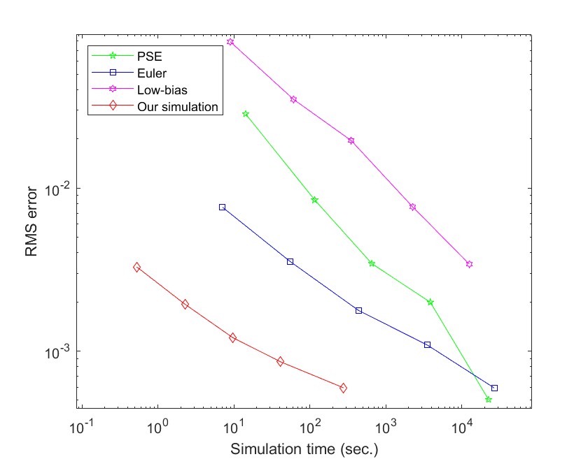
Based on the data points from Table 5, Figure 2 shows the plots of the trade-off between CPU time and RMS error. The figure explicitly demonstrates that, while the decay is slightly slower than the competing schemes, our simulation method achieves the same degree of RMS error using much less computation time, only about one hundredth of the Euler scheme. Thanks to the high efficiency for small time step , our algorithm is also effective for evaluating path-dependent options with frequent discrete monitoring.
5.3 Comparison with Islah’s approximation
In this last numerical experiment using Case V, we demonstrate superiority of our CEV approximation of conditional in Section 4.1 to Islah’s approximation which has been commonly adopted in other schemes. The parameter set is also taken from Cai et al. (2017, Figure 4). We price the at-the-money European option for maturity, with time step or 1. On one hand, our simulation scheme consists of (i) SLN sampling of and (ii) CEV model sampling of conditional . On the other hand, we replace the second step with Islah’s approximation (Proposition 8).
Under Islah’s approximation, a power transformation of observes a CEV distribution; see Eq. (22). Therefore, Kang (2014)’s algorithm also provides a better way to simulate Islah’s approach. Accordingly, we use Algorithm 1 with , , and replaced by , , and in Eq. (22), respectively, to sample . Then, is finally obtained.
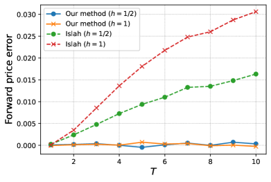
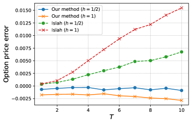
Figure 3 compares the results from the two approaches: our conditional distribution of and Islah’s approximation. Figure 3(a) shows the error of the terminal price , which should be equal to in theory. As expected, the results show that our approach preserves the martingale property fairly well for all time-to-maturity . That is, holds with very high accuracy regardless of . In Islah’s approach, however, deviates from . In particular, the deviation accumulates as the time-to-maturity becomes longer. The time step has to be smaller to reduce the deviation.
Figure 3(b) shows the error of the ATM option price from its true value computed with the FDM. Our approach is more accurate than Islah’s approach. Note that the higher option price error in Islah’s approach is due to failure of the martingale property. As the delta of ATM option is about 0.5, the option price error is approximately half of the forward price error. Conversely, the martingale preservation of our CEV approximation indeed improves European call option pricing. The option price error in our approach is mostly attributed to the error in distribution. The underpricing of option seems to be related to that the ex-kurtosis of sampled from the SLN approach, which is slightly smaller than that of true distribution (see Figure 1). The error is reduced when a smaller is used.
From Figure 3(b), we observe that under the same approach to sample , and same size of time step , the results using our CEV distribution of are very close to the benchmark FDM results. However, the results of Islah’s approximation have larger numerical bias as gets longer. These results illustrate that our CEV approximation of the conditional is superior to Islah’s approximation.
6 Conclusion
The stochastic-alpha-beta-rho (SABR) model proposed by Hagan et al. (2002) has been widely adopted for pricing derivatives under the stochastic volatility framework. The corresponding simulation methods have been studied extensively. The naive time-discretization schemes, such as the Euler or Milstein schemes, suffer from non-negligible bias caused by the truncation of negative forward values even when a small time step is used. Although researchers proposed various simulation schemes that overcome the limitation of the time-discretization schemes, the schemes have their own limitations. In sampling conditional average variance, the schemes are riddled with either heavy computation (Cai et al., 2017; Leitao et al., 2017a) or inaccurate approximation over a large simulation step (Chen et al., 2012). In sampling conditional forward price, almost all methods adopt Islah (2009)’s NCX2 approximation that neither preserves martingale property nor provides efficient sampling algorithm.
This paper present a series of innovations on the SABR simulation. Firstly, we derive the first four moments of the conditional average variance analytically, and sample the conditional average variance via an SLN random variable fitted to the first three moments. Our sampling procedure is accurate for reasonably large time-to-maturity and fast in computation in comparison to the numerical inverse transform methods. Secondly, we propose a martingale-preserving CEV approximation for the conditional forward price that preserves the martingale property. Lastly, we sample the conditional forward price efficiently with the exact CEV sampling algorithm of Makarov and Glew (2010) and Kang (2014). Numerical results show that our methods are highly efficient and accurate even under challenging parameter values, like large time-to-maturity , when compared with other simulation methods.
Funding
The works of Lilian Hu and Yue Kuen Kwok are supported by the Guangzhou-HKUST (GZ) Joint Funding Program (Number 2024A03J0630).
Appendix A Conditional moments of
The conditional average variance is closely related to the exponential functional of BM, defined by
where is a standard Brownian motion. The derivation of Proposition 2 is based on the analytic conditional moments of the exponential functional of BM (Matsumoto and Yor, 2005, (5.4)):
The conditional average variance is expressed by conditional on the terminal location of the BM, :
Therefore, the conditional moments admit the following integral form:
where we apply the change of variable, , to obtain the second line, and integration by part to obtain the third line.
Using the following analytic integral
we obtain for ,
which will be useful in the derivation below. Here, we define in such a way that for any non-zero as .
Next, we evaluate . For , we obtain
For , using , we have
For , using , we obtain
For , using , we have
In addition, the expansion of the mean, coefficient of variance, skewness, and ex-kurtosis (see Remark 5) around are obtained as
Appendix B Sampling Islah’s approximation via a CEV distribution
Though Islah’s approximation is less than desirable, we show that Islah’s distribution of can be expressed as a power of a CEV random variable. Therefore, the CEV simulation algorithm in Section 4.2 can be applied to expedite the sampling.
Let us define
so that
As a result, the complementary CDF of Islah (2009)’s approximation is equivalently expressed by
and this implies that
| (22) |
In other words, a power of instead of itself, follows a CEV distribution under Islah’s approximation. Therefore, can be sampled as
Lastly, we obtain
References
- Abramowitz and Stegun (1972) Abramowitz, M., Stegun, I.A. (Eds.), 1972. Handbook of Mathematical Functions with Formulas, Graphs, and Mathematical Tables. New York. URL: https://www.math.hkbu.edu.hk/support/aands/toc.htm.
- Andersen (2008) Andersen, L., 2008. Simple and efficient simulation of the Heston stochastic volatility model. Journal of Computational Finance 11, 1–42. doi:10.21314/JCF.2008.189.
- Antonov and Spector (2012) Antonov, A., Spector, M., 2012. Advanced analytics for the SABR model. SSRN Electronic Journal URL: https://ssrn.com/abstract=2026350.
- Cai et al. (2017) Cai, N., Song, Y., Chen, N., 2017. Exact simulation of the SABR model. Operations Research 65, 931–951. doi:10.1287/opre.2017.1617.
- Chen et al. (2012) Chen, B., Oosterlee, C.W., Van Der Weide, H., 2012. A low-bias simulation scheme for the SABR stochastic volatility model. International Journal of Theoretical and Applied Finance 15, 1250016. doi:10.1142/S0219024912500161.
- Choi et al. (2019) Choi, J., Liu, C., Seo, B.K., 2019. Hyperbolic normal stochastic volatility model. Journal of Futures Markets 39, 186–204. doi:10.1002/fut.21967.
- Choi and Wu (2021a) Choi, J., Wu, L., 2021a. The equivalent constant-elasticity-of-variance (CEV) volatility of the stochastic-alpha-beta-rho (SABR) model. Journal of Economic Dynamics and Control 128, 104143. doi:10.1016/j.jedc.2021.104143.
- Choi and Wu (2021b) Choi, J., Wu, L., 2021b. A note on the option price and ‘Mass at zero in the uncorrelated SABR model and implied volatility asymptotics’. Quantitative Finance 21, 1083–1086. doi:10.1080/14697688.2021.1876908.
- Cox (1996) Cox, J.C., 1996. The Constant Elasticity of Variance Option Pricing Model. The Journal of Portfolio Management 23, 15–17. doi:10.3905/jpm.1996.015.
- Cui et al. (2018) Cui, Z., Kirkby, J., Nguyen, D., 2018. A general valuation framework for SABR and stochastic local volatility models. SIAM Journal on Financial Mathematics 9, 520–563. doi:10.1137/16M1106572.
- Cui et al. (2021) Cui, Z., Kirkby, J.L., Nguyen, D., 2021. Efficient simulation of generalized SABR and stochastic local volatility models based on Markov chain approximations. European Journal of Operational Research 290, 1046–1062. doi:10.1016/j.ejor.2020.09.008.
- Derman and Kani (1998) Derman, E., Kani, I., 1998. Stochastic Implied Trees: Arbitrage Pricing with Stochastic Term and Strike Structure of Volatility. International Journal of Theoretical and Applied Finance 01, 61–110. doi:10.1142/S0219024998000059.
- Dupire (1997) Dupire, B., 1997. Pricing and hedging with smiles, in: Dempster, M.A.H., Pliska, S.R. (Eds.), Mathematics of Derivative Securities. number 15 in Publications of the Newton Institute, pp. 103–111.
- Fang and Oosterlee (2008) Fang, F., Oosterlee, C., 2008. A Novel Pricing Method for European Options Based on Fourier-Cosine Series Expansions. SIAM Journal on Scientific Computing 31, 826–848. doi:10.1137/080718061.
- Grzelak et al. (2019) Grzelak, L.A., Witteveen, J.A.S., Suárez-Taboada, M., Oosterlee, C.W., 2019. The stochastic collocation Monte Carlo sampler: Highly efficient sampling from ‘expensive’ distributions. Quantitative Finance 19, 339–356. doi:10.1080/14697688.2018.1459807.
- Gulisashvili et al. (2018) Gulisashvili, A., Horvath, B., Jacquier, A., 2018. Mass at zero in the uncorrelated SABR model and implied volatility asymptotics. Quantitative Finance 18, 1753–1765. doi:10.1080/14697688.2018.1432883.
- Hagan et al. (2002) Hagan, P.S., Kumar, D., Lesniewski, A.S., Woodward, D.E., 2002. Managing smile risk. Wilmott September, 84–108.
- Islah (2009) Islah, O., 2009. Solving SABR in Exact Form and Unifying it with LIBOR Market Model. SSRN Electronic Journal doi:10.2139/ssrn.1489428.
- Kang (2014) Kang, C., 2014. Simulation of the shifted Poisson distribution with an application to the CEV model. Management Science and Financial Engineering 20, 27–32. doi:10.7737/MSFE.2014.20.1.027.
- Kennedy et al. (2012) Kennedy, J.E., Mitra, S., Pham, D., 2012. On the Approximation of the SABR Model: A Probabilistic Approach. Applied Mathematical Finance 19, 553–586. doi:10.1080/1350486X.2011.646523.
- Kyriakou et al. (2023) Kyriakou, I., Brignone, R., Fusai, G., 2023. Unified Moment-Based Modeling of Integrated Stochastic Processes. Operations Research doi:10.1287/opre.2022.2422.
- Leitao et al. (2017a) Leitao, Á., Grzelak, L.A., Oosterlee, C.W., 2017a. On a one time-step Monte Carlo simulation approach of the SABR model: Application to European options. Applied Mathematics and Computation 293, 461–479. doi:10.1016/j.amc.2016.08.030.
- Leitao et al. (2017b) Leitao, Á., Grzelak, L.A., Oosterlee, C.W., 2017b. On an efficient multiple time step Monte Carlo simulation of the SABR model. Quantitative Finance 17, 1549–1565. doi:10.1080/14697688.2017.1301676.
- Lorig et al. (2017) Lorig, M., Pagliarani, S., Pascucci, A., 2017. Explicit implied volatilities for multifactor local-stochastic volatility models. Mathematical Finance 27, 926–960. doi:10.1111/mafi.12105.
- Makarov and Glew (2010) Makarov, R.N., Glew, D., 2010. Exact simulation of Bessel diffusions. Monte Carlo Methods and Applications 16, 283–306. doi:10.1515/mcma.2010.010, arXiv:0910.4177.
- Matsumoto and Yor (2005) Matsumoto, H., Yor, M., 2005. Exponential functionals of Brownian motion, I: Probability laws at fixed time. Probability Surveys 2, 312–347. doi:10.1214/154957805100000159.
- Obłój (2007) Obłój, J., 2007. Fine-tune your smile: Correction to Hagan et al. arXiv:0708.0998 [math, q-fin] URL: https://arxiv.org/abs/0708.0998, arXiv:0708.0998.
- Paulot (2015) Paulot, L., 2015. Asymptotic implied volatility at the second order with application to the SABR model, in: Friz, P., Gatheral, J., Gulisashvili, A., Jacquier, A., Teichmann, J. (Eds.), Large Deviations and Asymptotic Methods in Finance, pp. 37–69. doi:10.1007/978-3-319-11605-1_2.
- Schroder (1989) Schroder, M., 1989. Computing the constant elasticity of variance option pricing formula. Journal of Finance 44, 211–219. doi:10.1111/j.1540-6261.1989.tb02414.x.
- Yang et al. (2017) Yang, N., Chen, N., Liu, Y., Wan, X., 2017. Approximate arbitrage-free option pricing under the SABR model. Journal of Economic Dynamics and Control 83, 198–214. doi:10.1016/j.jedc.2017.08.004.