On determinant of checkerboard colorable virtual knots

Abstract.

For classical knots, it is well known that their determinants mod $8$ are classified by the Arf invariant. Boden and Karimi introduced a determinant of checkerboard colorable virtual knots. We prove that their determinant mod $8$ is classified by the coefficient of $z^{2}$ in the ascending polynomial which is an extension of the Conway polynomial for classical knots.

1. Introduction

For a knot in $S^{3}$, let $\Delta_{K}(t)$ denote the Conway-normalized Alexander polynomial, that is, $\Delta_{K}(t)=\det(t^{1/2}V-t^{-1/2}V^{T})$ for a Seifert matrix $V$ of $K$. The absolute value $\det K=|\Delta_{K}(-1)|$ is called the determinant of $K$. Here $\Delta_{K}(t)$ is related to the Conway polynomial $\nabla_{K}(z)$ of $K$ via $\Delta_{K}(t)=\nabla_{K}(t^{-1/2}-t^{1/2})$. Let $\operatorname{Arf}K\in\mathbb{Z}/2\mathbb{Z}$ denote the Arf invariant of $K$. Then, it is well known that

$$\det K\equiv\begin{cases}\pm 1\mod 8&\text{if $\operatorname{Arf}K=0$,}\\ \pm 3\mod 8&\text{if $\operatorname{Arf}K=1$.}\end{cases}$$ (1.1)

Figure 1. A virtual knot diagram, the corresponding Gauss diagram, and (projection of) knot in a thickened torus.

In this paper, we extend the above classical result to a certain class of virtual knots. A virtual knot is a generalization of classical knots, defined by a virtual knot diagram containing both real and virtual crossings, or by a Gauss diagram as illustrated in Figure 1. It is also defined to be a certain equivalence class of a knot in $\Sigma\times[0,1]$, where $\Sigma$ is an orientable closed surface. For its precise definition and related topics, we refer the reader to [14], [2], [4], and [6].

Boden, Chrisman, and Karimi [1] introduced a determinant of a pair $(L,F)$, where $L$ is a link in $\Sigma\times[0,1]$ with $[L]=0$ in $H_{1}(\Sigma\times[0,1];\mathbb{Z}/2\mathbb{Z})$ and $F$ is a spanning surface for $L$. Their determinant can be applied to checkerboard colorable virtual links introduced by Kamada [13] since they admit spanning surfaces. Boden and Karimi [4] defined another determinant for these links, which is independent of the choice of a spanning surface. Now, it is natural to expect that the Arf invariant for classical knots can be extended to checkerboard colorable virtual knots so that the extension and the determinant in [4] fit into (1.1).

When a knot $K$ satisfies $[K]=0$ in $\mathbb{Z}$-coefficients and $F$ is a Seifert surface of $K$, the Arf invariant is defined for $(K,F)$ and used as an obstruction for virtual concordance of Seifert surfaces by Chrisman, Mukherjee [10] and Boden, Karimi [3]. The Arf invariant for $(K,F)$, however, does not satisfy (1.1) above (see Example 3.5). We here focus on the fact that $\operatorname{Arf}K=v_{2}(K)\bmod 2$ for classical knots $K$, where $v_{2}(K)$ denotes the coefficient of $z^{2}$ in the Conway polynomial $\nabla_{K}(z)$. For a Gauss diagram $G$ of a virtual knot with a basepoint $b$ on the circle disjoint from chords, let $\nabla_{\mathrm{asc}}(G_{b})(z)$ (resp. $\nabla_{\mathrm{des}}(G_{b})(z)$) denote the ascending (resp. descending) polynomial introduced by Chmutov, Khoury, and Rossi [7]. For classical knots, $\nabla_{\mathrm{asc}}(G_{b})(z)$ and $\nabla_{\mathrm{des}}(G_{b})(z)$ do not depend on the choice of a diagram and basepoint, and they coincide with the Conway polynomial.

We write $v_{2,1}(G_{b})$ (resp. $v_{2,2}(G_{b})$) for the coefficient of $z^{2}$ in $\nabla_{\mathrm{asc}}(G_{b})(z)$ (resp. $\nabla_{\mathrm{des}}(G_{b})(z)$) and show that they behave well for a certain class of virtual knots containing checkerboard colorable virtual knots as the case $p=2$.

Theorem 1.1.

Let $G$ be a Gauss diagram of a mod $p$ almost classical knot. Then, for $j=1,2$, $v_{2,j}(G_{b})\bmod p$ do not depend on the choice of a basepoint $b$. Moreover, $v_{2,1}(G_{b})\equiv v_{2,2}(G_{b})\bmod p$.

This theorem allows us to define $v_{2}(K)\in\mathbb{Z}/2\mathbb{Z}$ for checkerboard colorable virtual knots $K$ by $v_{2}(K)=v_{2,1}(G_{b})\equiv v_{2,2}(G_{b})\bmod 2$. The purpose of this paper is to prove the following relation between $\det K$ in [4] and our invariant $v_{2}(K)$.

Corollary 1.2.

Let $K$ be a checkerboard colorable virtual knot. Then,

$$\det K\equiv\begin{cases}\pm 1\mod 8&\text{if $v_{2}(K)=0$,}\\ \pm 3\mod 8&\text{if $v_{2}(K)=1$.}\end{cases}$$

Note here that a similar result for almost classical knots is mentioned in [3, Section 4], but the definition of the determinant is different from [4] and ours. This difference arises from that of Gordon-Litherland linking forms (see a discussion after [5, Definition 3.1]).

By Corollary 1.2, while the Arf invariant derived from Seifert matrices coincides with the coefficient of $z^{2}$ in the Conway polynomial mod $2$ in classical knot theory, they play different roles in virtual knot theory. The former is an obstruction for concordance and the latter controls the determinant mod $8$. Finally, this paper is based on the first author’s master thesis at Hiroshima University written in Japanese.

Acknowledgments

The authors would like to thank Noboru Ito, Kodai Wada, and Yuka Kotorii for their helpful comments. This study was supported in part by JSPS KAKENHI Grant Numbers JP20K14317 and JP23K12974.

2. Preliminaries

2.1. mod $p$ almost classical knots

We review basic definitions concerning virtual links according to [2]. A virtual link is an equivalence class of virtual link diagrams, where two diagrams $D$ and $D^{\prime}$ are equivalent if there exists a finite sequence of Reidemeister moves and virtual moves from $D$ to $D^{\prime}$. Also, $D$ and $D^{\prime}$ are said to be welded equivalent if they are related by the Reidemeister moves, virtual moves, and forbidden overpass move in [2, Figure 1]. A short arc (resp. long arc) of a virtual link diagram is an arc connecting two consecutive crossings (resp. two under-crossings). For instance, the diagram on the left of Figure 1 has six short arcs and two long arcs.

We recall the following definition from [2, Section 5].

Definition 2.1.

Let $p$ be a non-negative integer. A diagram $D$ of oriented virtual link is said to be mod $p$ Alexander numberable if there exists an assignment of integers to the short arcs of $D$ such that the four integers $\lambda_{a},\lambda_{b},\lambda_{c},\lambda_{d}$ around a crossing as illustrated in Figure 2 satisfy

• $\lambda_{b}\equiv\lambda_{c}$ and $\lambda_{a}\equiv\lambda_{d}\equiv\lambda_{b}+1\bmod p$ if the crossing is real,

• $\lambda_{a}=\lambda_{c}$ and $\lambda_{b}=\lambda_{d}$ if the crossing is virtual.

Moreover, an oriented virtual link $L$ is said to be mod $p$ almost classical if $L$ admits a mod $p$ Alexander numberable diagram. As special cases, a mod $2$ (resp. mod $0$) almost classical link is also said to be checkerboard colorable in [13] (resp. almost classical in [18]).

Figure 2. Colorings of short arcs around positive/negative crossings and virtual crossing.

Note that a checkerboard colorable virtual link actually admits a checkerboard coloring in the sense of [13, Section 2] or [8, Introduction].

Example 2.2.

The virtual knot in Figure 1 is not checkerboard colorable. Indeed, one can check that the diagram in Figure 1 is not mod $2$ Alexander numberable and the crossing number of this diagram is minimal, and thus [2, Theorem 8.3] implies that it is not checkerboard colorable.

In Green’s table [12], $K=4.90$ is checkerboard colorable as illustrated in Figure 3. On the other hand, one can see that it is not almost classical.

Recall here that every oriented virtual link is represented by a Gauss diagram, which is a chord diagram with oriented chords (called arrows) and with signs $+1$ or $-1$ assigned to each chord. See, for example, [7]. Throughout this paper, orientations of circles of Gauss diagrams (and arrow diagrams in Section 3) are assumed to be counterclockwise.

We recall from [2, Section 1] the definition of an index of a chord.

Definition 2.3.

Let $G$ be a Gauss diagram of a virtual knot. The index $I(c)\in\mathbb{Z}$ of a chord $c$ of $G$ with sign $\varepsilon$ is defined by $I(c)=\varepsilon(r_{+}-r_{-}+l_{-}-l_{+})$, where $r_{\pm}$ (resp. $l_{\pm}$) denote the numbers of chords with sign $\pm$ intersecting $c_{i}$ from left to right (resp. from right to left) when the head of $c$ is oriented up.

The following lemma is stated after Definition 5.1 in [2].

Lemma 2.4.

Let $G$ be a Gauss diagram of oriented virtual knot diagram $D$. Then $D$ is mod $p$ Alexander numberable if and only of $I(c)\equiv 0\bmod p$ for any chord $c$ of $G$.

The next result is shown in much the same way as [2, Theorem 6.1]. See also an argument written before Theorem 5.2 in [2].

Theorem 2.5.

For an oriented virtual link $L$, the following are equivalent.

1. $L$ is mod $p$ almost classical.

2. $[L]\in H(\Sigma\times[0,1];\mathbb{Z}/p\mathbb{Z})$ is trivial, where $\Sigma$ is a Carter surface of $K$.

Figure 3. A mod $2$ Alexander numbering of a diagram of $4.90$ and labels of crossings and long arcs.

2.2. Determinant for checkerboard colorable links

We recall from [4, Section 3] the definition of the coloring matrix.

Definition 2.6.

Let $D$ be a checkerboard colorable diagram with real crossings $c_{1},\dots,c_{n}$ and long arcs $a_{1},\dots,a_{m}$. The coloring matrix $B(D)=(b_{ij})$ is the $n\times m$ matrix such that $b_{ij}=1$ if $a_{j}$ is both the over-crossing arc and one of the under-crossing arcs at $c_{i}$, otherwise

$$b_{ij}=\begin{cases}2&\text{if $a_{j}$ is the over-crossing arc at $c_{i}$,}\\ -1&\text{if $a_{j}$ is one of an under-crossing arc at $c_{i}$,}\\ 0&\text{otherwise.}\end{cases}$$

Example 2.7.

For the labels of the diagram of $K=4.90$ on the right of Figure 3, we have

$$B(D)=\begin{pmatrix}1&-1&0&0\\ 1&0&0&-1\\ 2&0&-1&-1\\ 2&-1&-1&0\\ \end{pmatrix}.$$

Therefore, $\det K=1$ (see Definition 2.8).

Now, we can define a determinant, which is an essential ingredient of this paper.

Definition 2.8.

The determinant $\det L$ of checkerboard colorable virtual link $L$ is defined to be the absolute value of the determinant of an $(n-1)\times(n-1)$ minor of $B(D)$, which is well-defined due to [4, Proposition 3.1].

The determinant is actually an invariant of welded links since the coloring matrix is invariant under the forbidden overpass move in [2, Figure 1]. We use this fact in the proof of Lemma 4.3.

To show a kind of skein relation for $\det L$ in the next subsection, we give another interpretation of $\det L$ in terms of a mock Seifert matrix introduced in [5, Definition 3.5]. Let $\Sigma$ be an orientable closed surface. For disjoint oriented virtual knots $K_{1}$ and $K_{2}$ in $\Sigma\times[0,1]$, we define the virtual linking number $\mathrm{vlk}(K_{1},K_{2})\in\mathbb{Z}$ by the identity

$$[K_{2}]=\mathrm{vlk}(K_{1},K_{2})[\mu]\in H_{1}(\Sigma\times[0,1]\setminus K_{1},\Sigma\times\{1\};\mathbb{Z})\cong\mathbb{Z}.$$

We recall the Gordon-Litherland form $\mathcal{L}_{F}$ from [5]. Let $\widetilde{F}$ be the boundary of a neighborhood of $F\subset\Sigma\times[0,1]$ and $\pi\colon\widetilde{F}\to F$ be the induced double cover. One can define a transfer map $\tau\colon H_{1}(F;\mathbb{Z})\to H_{1}(\widetilde{F};\mathbb{Z})$, and then the Gordon-Litherland form $\mathcal{L}_{F}\colon H_{1}(F)\times H_{1}(F)\to\mathbb{Z}$ is defined by $\mathcal{L}_{F}(\alpha,\beta)=\mathrm{vlk}(\tau(\alpha),\beta)$.

Definition 2.9.

Let $L$ be a link in $\Sigma\times[0,1]$ with $[L]=0\in H_{1}(\Sigma\times[0,1];\mathbb{Z}/2\mathbb{Z})$ and let $F$ be a spanning surface for $L$, that is, $F$ is (not necessarily orientable) connected compact surface whose boundary is $L$. A matrix for the Gordon-Litherland form $\mathcal{L}_{F}$ associated with $F$ is called a mock Seifert matrix for $L$.

Let $L$ be a checkerboard colorable virtual link and $D$ a diagram of $L$. We write for $X$ the quotient space obtained from $\Sigma\times[0,1]$ by identifying $\Sigma\times\{1\}$ with a point. Let $X_{2}$ be the double cover of $X$ branched over $L$ and $X_{\infty}$ the infinite cyclic cover of $X\setminus L$. It is shown in [4, Section 3] that we can compute the first elementary ideal $\mathcal{E}_{1}$ of the Alexander module $H_{1}(X_{\infty};\mathbb{Z})$ over the ring $\mathbb{Z}[t,t^{-1}]$ from a matrix $A(D)$ obtained by Fox’s free derivative. As mentioned before Proposition 3.1 in [4], the coloring matrix $B(D)$ is obtained from $A(D)$ by substituting $t=-1$ (up to sign for any given row). Therefore, one can compute the first elementary ideal of $H_{1}(X_{2};\mathbb{Z})$ over the ring $\mathbb{Z}[-1]=\mathbb{Z}$ from $B(D)$. On the other hand, it is shown in [5, Theorem 3.9] that a mock Seifert matrix for $L$ is a presentation matrix of $H_{1}(X_{2};\mathbb{Z})$. Therefore, we obtain the following consequence (see [5, Remark 3.11]).

Proposition 2.10.

Let $S$ be a mock Seifert matrix for $L$. Then, $\det L=|{\det S}|$ holds.

Remark 2.11.

For almost classical oriented link $L$, the Alexander polynomial $\Delta_{L}(t)$ is defined in [2, Section 7] (see also [15]). It is shown in [4, Proposition 4.1] that $\det L=|\Delta_{L}(-1)|$ holds.

Example 2.12.

Let $K$ be the virtual knot $6.87548$ in Green’s table [12] (see also [2, Figure 20]). Using a Seifert surface in [9, Figure 14] as a spanning surface, we have

$$S=\begin{pmatrix}-2&-1&0&0\\ -1&2&1&0\\ 0&-1&0&1\\ 0&0&1&2\end{pmatrix},$$

which is also obtained by adding $V^{+}$ and $V^{-}$ in [9, Example (6.87548)]. Then one has $\det K=1$. Note that this result is compatible with [2, Table 2].

2.3. Skein relation

We prove a kind of skein relation for $\det L$ similar to [2, Theorem 7.11] for the Alexander polynomial of almost classical links. The idea of the proof is based on [11, Lemma 3].

Theorem 2.13.

Let $L_{+}$, $L_{-}$ and $L_{0}$ be oriented virtual links in Figure 4. Suppose that one of them is checkerboard colorable (then the others are also checkerboard colorable) and consider spanning surfaces in Figure 5. Then, mock Seifert matrices $S_{+}$, $S_{-}$, $S_{0}$ associated with the spanning surfaces satisfy

$$\det S_{+}-\det S_{-}=2\det S_{0}.$$

Figure 4. Oriented virtual links $L_{+}$, $L_{-}$, $L_{0}$ that are identical except within a $3$-ball.

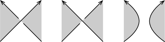
Figure 5. Spanning surfaces $F_{+}$, $F_{-}$, $F_{0}$ that are identical except within a $3$-ball.

Remark 2.14.

When $F_{0}$ is disconnected, we obtain a spanning surface by attaching a tube to $F_{0}$. The mock Seifert matrix for the resulting spanning surface satisfies Theorem 2.13 because then $\det S_{+}=\det S_{-}$ and $\det S_{0}=0$.

Proof of Theorem 2.13.

Fix a basis of $H_{1}(F_{0};\mathbb{Z})$ and let $S_{0}$ be the corresponding mock Seifert surface for $F_{0}$. Since $F_{+}$ is obtained from the connected surface $F_{0}$ by attaching a band, there exists a loop $\ell$ on $F_{+}$ passing through the band. By the Mayer-Vietoris exact sequence, the union of the basis of $H_{1}(F_{0};\mathbb{Z})$ and $[\ell]\in H_{1}(F_{+};\mathbb{Z})$ is a basis of $H_{1}(F_{+};\mathbb{Z})$. Now, the union also gives a basis of $H_{1}(F_{-};\mathbb{Z})$. Let $S_{\pm}$ be mock Seifert surfaces for $F_{\pm}$ with respect to the bases. Then one can see that

$$S_{+}=\begin{pmatrix}S_{0}&\bm{x}\\ \bm{y}^{T}&a\end{pmatrix},\quad S_{-}=\begin{pmatrix}S_{0}&\bm{x}\\ \bm{y}^{T}&a-2\end{pmatrix}$$

for some $a\in\mathbb{Z}$ and integral column vectors $\bm{x},\bm{y}$. We have

$$\det S_{-} =\det\begin{pmatrix}S_{0}&\bm{x}\\ \bm{y}^{T}&a-2\end{pmatrix}$$

$$=\det\begin{pmatrix}S_{0}&\bm{x}\\ \bm{y}^{T}&a\end{pmatrix}+\det\begin{pmatrix}S_{0}&\bm{0}\\ \bm{y}^{T}&-2\end{pmatrix}$$

$$=\det S_{+}-2\det S_{0}.$$

This completes the proof. ∎

3. Ascending and descending polynomials

We review basic definitions according to [7]. An arrow diagram is a based chord diagram with oriented chords (called arrows). A homomorphism $\varphi$ from $A$ to $G$ is an orientation-preserving homeomorphism of the circle of $A$ to the circle of $G$ which maps the basepoint to the basepoint and induces an injective map of arrows of $A$ to arrows of $G$ respecting the orientation of the arrows.

Definition 3.1.

For an arrow diagram $A$ and a based Gauss diagram $G$, define the pairing $\langle A,G\rangle\in\mathbb{Z}$ by

$$\langle A,G\rangle=\sum_{\varphi\in\mathrm{Hom}(A,G)}\prod_{\text{$\mathsf{a}$:\,arrow in $A$}}\operatorname{sign}(\varphi(\mathsf{a})).$$

Definition 3.2.

For a non-negative integer $n$, the Conway combination $\mathfrak{C}_{2n}$ (resp. $\mathfrak{C}^{\prime}_{2n}$) is defined to be the sum of one-component ascending (resp. descending) arrow diagrams with $2n$ arrows on a circle (see [7, Definition 4.3] for the definitions of one-component descending and ascending arrow diagrams). Similarly, $\mathfrak{C}_{2n+1}$ (resp. $\mathfrak{C}^{\prime}_{2n+1}$) is defined to be the sum of one-component ascending (resp. descending) diagrams with $2n+1$ arrows on two circles.

For instance, each of $\mathfrak{C}_{1}$, $\mathfrak{C}^{\prime}_{1}$, $\mathfrak{C}_{2}$, and $\mathfrak{C}^{\prime}_{2}$ consists of a single diagram illustrated in Figure 6.

Figure 6. Conway combinations $\mathfrak{C}_{1}$, $\mathfrak{C}^{\prime}_{1}$, $\mathfrak{C}_{2}$, and $\mathfrak{C}^{\prime}_{2}$.

Definition 3.3.

For a based Gauss diagram $G$, define the ascending polynomial $\nabla_{\mathrm{asc}}(G)(z)$ and descending polynomial $\nabla_{\mathrm{des}}(G)(z)\in\mathbb{Z}[z]$ respectively by

$$\nabla_{\mathrm{asc}}(G)(z)=\sum_{i\geq 0}\langle\mathfrak{C}_{2i},G\rangle z^{2i}\text{ and }\nabla_{\mathrm{des}}(G)(z)=\sum_{i\geq 0}\langle\mathfrak{C}^{\prime}_{2i},G\rangle z^{2i}.$$

Remark 3.4.

The polynomials $\nabla_{\mathrm{asc}}(G)(z)$ and $\nabla_{\mathrm{des}}(G)(z)$ depend on the choice of a basepoint of $G$ in general. For instance, one can observe it for the Gauss diagram in Figure 1. This is because the virtual knot in Figure 1 is not (mod $0$) almost classical, which implies that the assumption of Theorems 1.1 and 4.7 is essential in their proofs.

Example 3.5.

Let $K$ be the (almost classical) virtual knot $6.87548$ in Green’s table [12]. For the Gauss diagram in [9, Figure 14] (with an arbitrary basepoint), the coefficients of $z^{2}$ in $\nabla_{\mathrm{asc}}(G)(z)$ and in $\nabla_{\mathrm{des}}(G)(z)$ are $-2$. On the other hand, concerning determinant and Arf invariant in [3], one can see $\det(K,F)=5$ and $\operatorname{Arf}(q_{K,F})=1$. Indeed, these are computed from a Seifert matrix

$$V^{+}=\begin{pmatrix}-1&0&0&0\\ -1&1&1&0\\ 0&-1&0&1\\ 0&0&0&1\end{pmatrix}$$

written in [9, Example (6.87548)]. See also [3, Remark 3.5].

In [7, Lemma 5.1 and (5.3)], skein relations among pairings are shown for classical links. In their proofs, any property of classical knots is not used, and hence we obtain the following lemmas as extensions to virtual links.

Lemma 3.6.

Let $D_{+}$, $D_{-}$, $D_{0}$ be a skein triple drawn in Figure 4 such that $D_{\pm}$ have one component and $D_{0}$ has two components. Let $G_{+}$, $G_{-}$, $G_{0}$ be the corresponding Gauss diagrams. Then, for $n\geq 1$,

$$\langle\mathfrak{C}_{2n},G_{+}\rangle-\langle\mathfrak{C}_{2n},G_{-}\rangle =\langle\mathfrak{C}_{2n-1},G_{0}\rangle,$$

$$\langle\mathfrak{C}^{\prime}_{2n},G_{+}\rangle-\langle\mathfrak{C}^{\prime}_{2n},G_{-}\rangle =\langle\mathfrak{C}^{\prime}_{2n-1},G_{0}\rangle.$$

Lemma 3.7.

Let $D_{+}$, $D_{-}$, $D_{0}$ be a skein triple drawn in Figure 4 such that $D_{\pm}$ have two components and $D_{0}$ has one component. Let $G_{+}$, $G_{-}$, $G_{0}$ be the corresponding Gauss diagrams. Then, for $n\geq 0$,

$$\langle\mathfrak{C}_{2n+1},G_{+}\rangle-\langle\mathfrak{C}_{2n+1},G_{-}\rangle =\langle\mathfrak{C}_{2n},G_{0}\rangle,$$

$$\langle\mathfrak{C}^{\prime}_{2n+1},G_{+}\rangle-\langle\mathfrak{C}^{\prime}_{2n+1},G_{-}\rangle =\langle\mathfrak{C}^{\prime}_{2n},G_{0}\rangle.$$

The next notion is an extension of [17] to virtual knots, which will be used in the proof of Theorem 4.5.

Definition 3.8.

Let $D$ be a diagram of an oriented virtual knot with a basepoint. The warping degree $d(D)$ of $D$ is defined to be the number of crossings at which we first go through the under-arcs when we travel from the basepoint along the orientation of $D$. Moreover, the warping degree $d(G)$ of a based Gauss diagram $G$ is defined to be that of a virtual link diagram whose Gauss diagram is $G$.

A diagram $D$ is said to be descending if $d(D)=0$. It is shown in [16, Proposition 2.2] that a descending diagram is welded equivalent to the trivial one. This fact will be used in the proof of Lemma 4.3.

4. Main results

This section is devoted to proving Theorem 1.1 and Corollary 1.2. We first show some lemmas.

Lemma 4.1.

Let $G$ be a based Gauss diagram with $d(G)=0$. Then, for any positive integer $n$,

$$\langle\mathfrak{C}_{2n},G_{b}\rangle=\langle\mathfrak{C}^{\prime}_{2n},G_{b}\rangle=0.$$

Proof.

First, $\langle\mathfrak{C}_{2n},G_{b}\rangle=0$ is obvious by definition. Next, since $d(G)=0$, every descending subdiagram of $G$ is of the form in Figure 7. This is not one-component, and thus $\langle\mathfrak{C}^{\prime}_{2n},G_{b}\rangle=0$. ∎

Figure 7. Descending diagram with isolated $2n$ arrows.

Lemma 4.2.

Let $G_{b}$ be a based Gauss diagram of mod $p$ almost classical oriented virtual knot and let $\mathsf{a}$ be an arrow. The $\mathsf{a}$ divides the circle into two arcs and suppose that the tail of any arrow intersecting with $\mathsf{a}$ is attached to the arc containing $b$. Let $H_{b}$ be the $2$-component based Gauss diagram obtained by smoothing $G_{b}$ along $\mathsf{a}$. Then, $\langle\mathfrak{C}_{1},H_{b}\rangle\equiv\langle\mathfrak{C}^{\prime}_{1},H_{b}\rangle\equiv 0\bmod p$ and $\langle\mathfrak{C}_{2n-1},H_{b}\rangle=0$ for $n\geq 2$.

Proof.

First, $\langle\mathfrak{C}_{1},H_{b}\rangle=0$ is obvious by definition. Next, by Lemma 2.4, we have $\langle\mathfrak{C}_{1},H_{b}\rangle\equiv\langle\mathfrak{C}^{\prime}_{1},H_{b}\rangle\bmod p$. Let $H^{\prime}$ be a one-component subdiagram of $H_{b}$ with $2n-1$ arrows. $H^{\prime}$ must have an arrow connecting two circles of $H_{b}$. Since the tail of the arrow is attached to the circle containing $b$, $H^{\prime}$ is not ascending, and hence $\langle\mathfrak{C}_{2n-1},H_{b}\rangle=0$. ∎

Lemma 4.3.

Let $K$ be a checkerboard colorable virtual knot admitting a descending diagram. Then, $\det K=1$.

Proof.

First, a descending diagram is welded equivalent to the trivial one by [16, Proposition 2.2]. Since $\det K$ is invariant under welded equivalence, we conclude that $\det K=1$. ∎

Lemma 4.4.

Let $L=L_{1}\cup L_{2}$ be $2$-component mod $2$ almost classical oriented virtual link. If $L$ admits a diagram $D=D_{1}\cup D_{2}$ such that $D_{1}$ is above $D_{2}$ at every crossing between them, then $\det L=0$.

Proof.

Let $c_{1},\dots,c_{k}$ be the real crossings of $D_{1}$ and itself, and let $c_{k+1},\dots,c_{n}$ be the rest of real crossings of $D$. We may assume $k\geq 1$ and $n\geq 2$ by Reidemeister moves. Let $a_{1},\dots,a_{l}$ be long arcs of $D_{1}$ and let $a_{l+1},\dots,a_{m}$ be that of $D_{2}$. The assumption implies $k=l$ and we have

$$B(D)=\begin{pmatrix}B(D_{1})&O\\ \ast&\ast\end{pmatrix}.$$

Since $\det B(D_{1})=0$ (see a sentence before [4, Proposition 3.1]), any $(n-1)\times(n-1)$ minor of $B(D)$ is zero. ∎

Theorem 4.5.

Let $K$ be a checkerboard colorable oriented virtual knot, $G$ a based Gauss diagram of $K$, and $S$ a mock Seifert matrix for $K$. Then, $\det S\equiv\pm\nabla_{\mathrm{asc}}(G)(2)\bmod 8$.

Proof.

For non-negative integers $n$, we introduce the following proposition $(\ast)_{n}$ which is a refinement of the statement above.

$(\ast)_{n}$:

Let $D$ be a diagram of a checkerboard colorable oriented virtual knot with $n$ real crossings, $G$ the Gauss diagram corresponding to $D$ with an arbitrary basepoint, and $S$ a mock Seifert matrix for $K$. Then, $\det S\equiv\pm\nabla_{\mathrm{asc}}(G)(2)\bmod 8$. Moreover, let $D_{0}$ be a diagram of $2$-component link obtained by smoothing a real crossing of a diagram of a checkerboard colorable oriented virtual knot with $n+1$ real crossings, $G_{0}$ a based Gauss diagram of $D_{0}$, and $S_{0}$ a mock Seifert matrix for the link represented by $D_{0}$. Then, $\det S_{0}\equiv\pm\nabla_{\mathrm{asc}}(G_{0})(2)\bmod 4$.

We prove $(\ast)_{n}$ by induction on $n$. First, $(\ast)_{0}$ is true since a virtual knot without real crossings is the unknot and the link obtained from a knot with a single real crossing by smoothing the crossing is a trivial link.

We next assume that $(\ast)_{n-1}$ is true and we prove

$$\det S\equiv\pm\nabla_{\mathrm{asc}}(G)(2)\bmod 8$$ (4.1)

by induction on the warping degree $d$ of $G$. If $d=0$, then $D$ is descending, and thus (4.1) holds by Lemmas 4.3 and 4.1. Assume that (4.1) holds when the warping degree is less than $d$. Let $D$ and $S$ be a diagram and matrix in $(\ast)_{n}$ and assume $d(G)=d$.

Let $\mathsf{a}$ be an arrow of $G$. By smoothing $G$ along $\mathsf{a}$, we obtain diagrams $G^{\prime}$ and $G_{0}$. Since $d(G^{\prime})=d-1$, one has $\det S^{\prime}\equiv\varepsilon^{\prime}\nabla_{\mathrm{asc}}(G^{\prime})(2)\bmod 8$ for some $\varepsilon^{\prime}\in\{\pm 1\}$. By $(\ast)_{n-1}$, we have $\det S_{0}\equiv\pm\nabla_{\mathrm{asc}}(G_{0})(2)\bmod 4$. Let $\varepsilon$ be the sign of the crossing. Using Lemma 3.6, we have

$$\det S =\det S^{\prime}+\varepsilon 2\det S_{0}$$

$$\equiv\varepsilon^{\prime}\nabla_{\mathrm{asc}}(G^{\prime})(2)+2\varepsilon\nabla_{\mathrm{asc}}(G_{0})(2)\mod 8$$

$$\equiv\varepsilon^{\prime}\nabla_{\mathrm{asc}}(G^{\prime})(2)+2\varepsilon^{\prime}\varepsilon\nabla_{\mathrm{asc}}(G_{0})(2)\mod 8$$

$$\equiv\varepsilon^{\prime}\nabla_{\mathrm{asc}}(G)(2)\mod 8.$$

Here the third equality follows from

$$\nabla_{\mathrm{asc}}(G_{0})(2)=\sum_{i\geq 1}\langle\mathfrak{C}_{2i-1},G_{0}\rangle 2^{2i-1}\equiv\varepsilon^{\prime}\nabla_{\mathrm{asc}}(G_{0})(2)\mod 4.$$

We finally prove

$$\det S_{0}\equiv\pm\nabla_{\mathrm{asc}}(G_{0})(2)\bmod 4$$ (4.2)

by induction on the number $k$ of arrows in $G$ from the component without basepoint to the other component. If $k=0$, then one component of $D_{0}$ is above the other component at every real crossing, and thus (4.2) holds by Lemmas 4.2 and 4.4. Assume (4.2) holds less than $k$. Let $S_{0}$ and $G_{0}$ be a matrix and diagram in $(\ast)_{n}$, respectively. Let $\mathsf{a}$ be an arrow in $G$ from the component without basepoint to the other component. Let $D_{0}^{\prime}$ and $D_{0}^{0}$ be diagrams obtained by crossing change and smoothing at the crossing corresponding to $\mathsf{a}$. By the induction hypothesis, we have $\det S_{0}^{\prime}\equiv\varepsilon^{\prime}\nabla_{\mathrm{asc}}(G_{0}^{\prime})(2)\bmod 4$ for some $\varepsilon^{\prime}\in\{\pm 1\}$. By $(\ast)_{n-1}$, we have $\det S_{0}^{0}\equiv\nabla_{\mathrm{asc}}(G_{0}^{0})(2)\mod 8$. Using Theorem 2.13, we have

$$\det S^{0} =\det S_{0}^{\prime}+\varepsilon 2\det S_{0}^{0}$$

$$\equiv\varepsilon^{\prime}\nabla_{\mathrm{asc}}(G_{0}^{\prime})(2)+2\varepsilon\nabla_{\mathrm{asc}}(G_{0}^{0})(2)\mod 4$$

$$\equiv\varepsilon^{\prime}\nabla_{\mathrm{asc}}(G_{0}^{\prime})(2)+2\varepsilon^{\prime}\varepsilon\nabla_{\mathrm{asc}}(G_{0}^{0})(2)\mod 4$$

$$\equiv\varepsilon^{\prime}\nabla_{\mathrm{asc}}(G_{0})(2)\mod 4,$$

where the last equality follows from Lemma 3.7. ∎

Now, we divide Theorem 1.1 into the following two theorems and give their proofs.

Theorem 4.6.

Let $G$ be a based Gauss diagram of a mod $p$ almost classical oriented knot. Then, $\langle\mathfrak{C}_{2},G\rangle\equiv\langle\mathfrak{C}^{\prime}_{2},G\rangle\bmod p$.

Proof.

The proof is by induction on the pair $(n(G),d(G))$, where we write $n(G)$ for the number of arrows of $G$ in this proof. In the case $(n(G),d(G))=(0,0)$, we see $\langle\mathfrak{C}_{2},G\rangle=\langle\mathfrak{C}^{\prime}_{2},G\rangle=0$. Assume that it holds for $G$ such that $(n(G),d(G))$ is smaller than a given $(n,d)$ in the lexicographic order. Let $G$ be a Gauss diagram of a mod $p$ almost classical oriented knot with $(n(G),d(G))=(n,d)$. If $d(G)=0$, Lemma 4.1 implies $\langle\mathfrak{C}_{2},G\rangle\equiv\langle\mathfrak{C}^{\prime}_{2},G\rangle\bmod p$.

Consider the case $d(G)\geq 1$. Then there exists an arrow $\mathsf{a}$ such that the head of $\mathsf{a}$ appears before the tail when we move on the circle from $b$. Let $G_{\mathsf{a}}^{\prime}$ (resp. $G_{\mathsf{a}}^{0}$) be the diagram obtained from $G$ by switching the orientation of $\mathsf{a}$ (resp. smoothing along $\mathsf{a}$). By Lemma 3.6, we have

$$\langle\mathfrak{C}_{2},G\rangle=\langle\mathfrak{C}_{2},G_{\mathsf{a}}^{\prime}\rangle+\varepsilon\langle\mathfrak{C}_{1},G_{\mathsf{a}}^{0}\rangle,$$

$$\langle\mathfrak{C}^{\prime}_{2},G\rangle=\langle\mathfrak{C}^{\prime}_{2},G_{\mathsf{a}}^{\prime}\rangle+\varepsilon\langle\mathfrak{C}^{\prime}_{1},G_{\mathsf{a}}^{0}\rangle.$$

for some $\varepsilon\in\{\pm 1\}$. By the induction hypothesis and $I(\mathsf{a})\equiv 0\bmod p$, we conclude that $\langle\mathfrak{C}_{2},G\rangle\equiv\langle\mathfrak{C}^{\prime}_{2},G\rangle\bmod p$. ∎

Figure 8. Ascending diagrams with basepoints $b$ and $b^{\prime}$.

Theorem 4.7.

Let $G$ be a Gauss diagram of a mod $p$ almost classical oriented knot. Then $\langle\mathfrak{C}_{2},G_{b}\rangle\bmod p$ and $\langle\mathfrak{C}^{\prime}_{2},G_{b}\rangle\bmod p$ do not depend on the choice of a basepoint $b$.

Proof.

By Theorem 4.6, we need to discuss only $\langle\mathfrak{C}_{2},G_{b}\rangle\bmod p$. It suffices to show that $\langle\mathfrak{C}_{2},G_{b}\rangle\equiv\langle\mathfrak{C}_{2},G_{b^{\prime}}\rangle\bmod 2$, where the basepoint $b$, an endpoint of an arrow $\mathsf{a}$, and $b^{\prime}$ are aligned in this order on the oriented circle. We use the same symbols $r_{\pm}$ and $l_{\pm}$ as Definition 2.3 with respect to $\mathsf{a}$ with sign $\varepsilon$. There are two cases where the above endpoint of $\mathsf{a}$ between $b$ and $b^{\prime}$ is (I) the head or (II) the tail of $\mathsf{a}$.

In the case (I), the contribution of subdiagrams containing $\mathsf{a}$ in $\langle\mathfrak{C}_{2},G_{b}\rangle$ (resp. $\langle\mathfrak{C}_{2},G_{b^{\prime}}\rangle$) is $\varepsilon(r_{+}-r_{-})$ (resp. $\varepsilon(l_{+}-l_{-})$) as drawn in Figure 8. They are the same mod $p$ by Lemma 2.4. Since the contribution of subdiagrams which do not contain $\mathsf{a}$ in $\langle\mathfrak{C}_{2},G_{b}\rangle$ is the same as that of $\langle\mathfrak{C}_{2},G_{b^{\prime}}\rangle$, we conclude that $\langle\mathfrak{C}_{2},G_{b}\rangle\equiv\langle\mathfrak{C}_{2},G_{b^{\prime}}\rangle\bmod 2$.

In the case (II), there is no subdiagram containing $\mathsf{a}$ which contributes to $\langle\mathfrak{C}_{2},G_{b}\rangle$. Therefore, we complete the proof. ∎

Proof of Corollary 1.2.

Let $G$ be a based Gauss diagram of a checkerboard colorable virtual knot $K$. It follows from Theorems 4.5 and 1.1 that

$$\det K =\pm\nabla_{\mathrm{asc}}(G)(2)=\pm\sum_{i\geq 0}\langle\mathfrak{C}_{2i},G\rangle 2^{2i}$$

$$\equiv\pm 1+\langle\mathfrak{C}_{2},G\rangle 4\equiv\pm 1+4v_{2}(K)\mod 8.$$

This completes the proof. ∎

Theorem 1.1 and Corollary 1.2 reveal important properties of the second-degree term of the ascending/descending polynomial for checkerboard colorable virtual knots. On the other hand, higher degree terms of the ascending/descending polynomial are not necessarily well known. It is natural to investigate their properties and applications.

References

- [1] H. U. Boden, M. Chrisman, and H. Karimi. The Gordon-Litherland pairing for links in thickened surfaces. Internat. J. Math., 33(10-11):Paper No. 2250078, 47, 2022.
- [2] H. U. Boden, R. Gaudreau, E. Harper, A. J. Nicas, and L. White. Virtual knot groups and almost classical knots. Fund. Math., 238(2):101–142, 2017.
- [3] H. U. Boden and H. Karimi. Concordance invariants of null-homologous knots in thickened surfaces. arXiv:2111.07409v1, 2021.
- [4] H. U. Boden and H. Karimi. Classical results for alternating virtual links. New York J. Math., 28:1372–1398, 2022.
- [5] H. U. Boden and H. Karimi. Mock seifert matrices and unoriented algebraic concordance. arXiv:2301.05946v3, 2023.
- [6] S. Chmutov, S. Duzhin, and J. Mostovoy. Introduction to Vassiliev knot invariants. Cambridge University Press, Cambridge, 2012.
- [7] S. Chmutov, M. C. Khoury, and A. Rossi. Polyak-Viro formulas for coefficients of the Conway polynomial. J. Knot Theory Ramifications, 18(6):773–783, 2009.
- [8] S. Chmutov and I. Pak. The Kauffman bracket of virtual links and the Bollobás-Riordan polynomial. Mosc. Math. J., 7(3):409–418, 573, 2007.
- [9] M. Chrisman. Virtual Seifert surfaces. J. Knot Theory Ramifications, 28(6):1950039, 33, 2019.
- [10] M. Chrisman and S. Mukherjee. Algebraic concordance order of almost classical knots. J. Knot Theory Ramifications, 32(11):Paper No. 2350072, 34, 2023.
- [11] C. A. Giller. A family of links and the Conway calculus. Trans. Amer. Math. Soc., 270(1):75–109, 1982.
- [12] J. Green. A table of virtual knots. https://www.math.toronto.edu/drorbn/Students/GreenJ/.
- [13] N. Kamada. On the Jones polynomials of checkerboard colorable virtual links. Osaka J. Math., 39(2):325–333, 2002.
- [14] L. H. Kauffman. Virtual knot theory. European J. Combin., 20(7):663–690, 1999.
- [15] T. Nakamura, Y. Nakanishi, S. Satoh, and Y. Tomiyama. Twin groups of virtual 2-bridge knots and almost classical knots. J. Knot Theory Ramifications, 21(10):1250095, 18, 2012.
- [16] S. Satoh. Crossing changes, delta moves and sharp moves on welded knots. Rocky Mountain J. Math., 48(3):967–979, 2018.
- [17] A. Shimizu. The warping degree of a knot diagram. J. Knot Theory Ramifications, 19(7):849–857, 2010.
- [18] D. S. Silver and S. G. Williams. Crowell’s derived group and twisted polynomials. J. Knot Theory Ramifications, 15(8):1079–1094, 2006.