Channel-Aware Distributed Transmission Control and Video Streaming in UAV Networks

Abstract

In this paper, we study the problem of distributed transmission control and video streaming optimization for unmanned aerial vehicles (UAVs) operating in unlicensed spectrum bands. We develop a rigorous cross-layer analysis framework that jointly considers three inter-dependent factors: (i) in-band interference introduced by ground/aerial nodes at the physical (PHY) layer, (ii) limited-size queues with delay-constrained packet arrival at the medium access control (MAC) layer, and (iii) video encoding rate at the application layer. First, we formulate an optimization problem to maximize the throughput by optimizing the fading threshold. To this end, we jointly analyze the queue-related packet loss probabilities (i.e., buffer overflow and time threshold event) as well as the outage probability due to the low signal-to-interference-plus-noise ratio (SINR). We introduce the Distributed Transmission Control (DTC) algorithm that maximizes the throughput by adjusting transmission policies to balance the trade-offs between packet drop from queues vs. transmission errors due to low SINRs. Second, we incorporate the video distortion model to develop distributed peak signal-to-noise ratio (PSNR) optimization for video streaming. The formulated optimization incorporates two cross-layer parameters, specifically the fading threshold and video encoding rate. To tackle this problem, we develop the Joint Distributed Video Transmission and Encoder Control (JDVT-EC) algorithm that enhances the PSNR for all nodes by fine-tuning transmission policies and video encoding rates to balance the trade-offs between packet loss and lossy video compression distortions. Through extensive numerical analysis, we thoroughly examine the proposed algorithms and demonstrate that they are able to find the optimal transmission policies and video encoding rates under various scenarios.

I Introduction

Recently, UAV-enabled wireless communication has shown promising applications due to ease of deployment, high agility, ability to perform different tasks, and the high probability of establishing Line-of-Sight (LoS) links with ground/aerial nodes. For example, they can provide video streaming services in areas with limited infrastructure, such as disaster-affected areas where ground base stations (BSs) may be nonfunctional or during periods of overloaded video traffic in existing cellular networks [1]. In fact, the capability of UAVs for video streaming plays a crucial role in public safety applications [2], as they can be deployed in search and rescue operations to efficiently cover large areas and provide live videos to locate missing persons or assess disaster areas. During emergencies, UAVs’ live videos enable commanders to facilitate quick decision-making about resource allocation and response strategies [3]. To realize these benefits, both licensed and unlicensed spectrum bands can be used for UAV communications. Licensed bands offer exclusive access but have regulatory obligations, while unlicensed bands are shared and more prone to interference [4]. This poses challenges for reliable UAV communication and video streaming. To address this, developing distributed video streaming and transmission control policies is crucial to ensure high quality of experience (QoE), particularly for UAVs that depend on time-sensitive video packets and command-and-control (C2) data [5, 6].

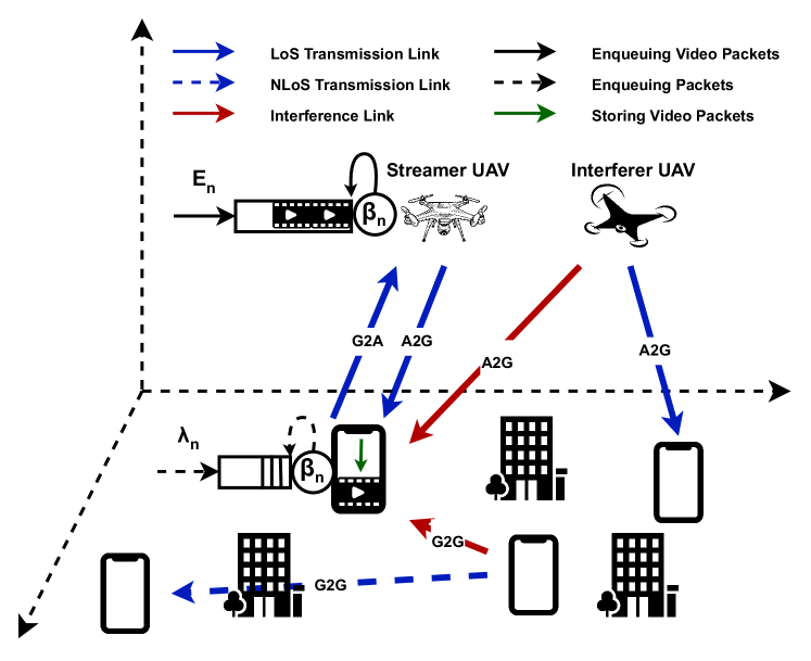
Figure 1: System model including aerial and ground nodes operating in unlicensed spectrum bands. The proposed system model captures in-band interference, limited-size queues with delay-constrained traffic and video streaming between the streamer UAV and its associated ground node.

Extensive research has been conducted on various aspects of UAV networking (see, for example, [7, 8, 9]). However, several research gaps remain in developing distributed transmission policies that jointly consider (i) interference levels in unlicensed spectrum bands, (ii) transmission queue states regarding buffer size and queuing delay, and (iii) video encoding rate optimization. For example, [10] models LoS and Non-LoS (NLoS) wireless links for UAVs and defines a transmission policy without considering interference. In [11], a distributed transmission policy is developed for ground-level terrestrial networks only, and not specifically for UAV networks. The study in [12] proposes a new LoS channel model for UAVs, but does not include an interference model in the outage probability. In [13], ground-to-air (G2A) and air-to-ground (A2G) channels are modeled, and system performance is characterized in terms of UAV trajectory rather than channel parameters. Therefore, although there has been research on UAV network transmission policies [10, 12, 13], a comprehensive investigation of distributed policies that consider packet queues, interference levels, and video encoding rates in unlicensed bands is still lacking.

This paper aims to address this gap by exploring how UAVs and ground-level nodes achieve an optimal policy by adjusting the fading threshold and video encoding rate in a distributed manner to achieve optimal throughput and PSNR performance metrics. To this end, we formulate two optimization problems to maximize the throughput and PSNR performance, which is used to measure the quality of video frames. To solve the formulated problems, we first propose the Distributed Transmission Control (DTC) algorithm that determines the optimal fading threshold set $\boldsymbol{\beta}^{\star}$ in the environment to maximize the average throughput for all nodes. Next, to solve the video streaming problem, we develop the Joint Distributed Video Transmission and Encoder Control (JDVT-EC) algorithm that optimizes average PSNR for all nodes by adjusting transmission policies and video encoding rates to balance the trade-offs between packet loss and lossy video compression distortions. Through comprehensive numerical results, we compare the performance of our proposed algorithms with several baselines, confirming the effectiveness of our method. In summary, the main contributions of this paper are as follows.

• We propose a comprehensive analytical framework to develop PSNR-optimal distributed video streaming and throughput-optimal distributed packet transmission for UAV networks. Our framework considers the impacts of buffer overflow and time threshold losses in the queue, transmission error loss in the channel as an overall packet loss within the MAC and PHY layers, and the effect of video encoding rate as a video distortion within the application layer. Based on this cross-layer scheme, we compute the throughput and PSNR for video streaming UAV networks.

• We develop optimization algorithms to control the distributed transmission policy in the presence of interferer nodes and distributed encoder control. We employ the consensus-based distributed optimization and coordinate descent optimization to achieve the optimal fading threshold and video encoding rate for maximizing the average throughput and PSNR over all nodes.

• We implement our proposed algorithms and evaluate their efficacy extensively under various scenarios compared to several baseline policies. Also, we show the average optimal PSNR for a specific spatial area between a ground node and the streamer UAV.

The rest of this paper is organized as follows. In Section II, the related work is presented. Section III describes the system model, including the wireless channel model and transmission policies. In Section IV, we formulate the distributed transmission control problem in terms of queue and interference analysis for throughput optimization. Section V investigates the distortion-based PSNR optimization problem. In Section VI, extensive numerical results are provided, followed by the conclusion in Section VII.

II Related Work

We discuss related works by dividing our analysis into two main categories: distributed transmission control and video streaming optimization for UAVs.

Distributed Transmission Control. In this section, we review related works focused on developing distributed transmission control policies as well as cross-layer solutions. Wang et al. [14] proposed a closed-form expression for the average packet error probability and effective throughput of the control link in UAV communication. Their framework considers a ground central station (GCS) that transmits control signals toward the UAV to ensure ultra-reliable and low-latency communication (URLLC). Solanki et al. [15] proposed a C2 short packet communication from a multi-antenna GCS to UAV. They derived a closed-form expression for the average block error rate and formulated a joint optimization problem to maximize the UAV coverage range to be reliably controlled by GCS. Ultimately, they solved this problem using standard convex optimization solvers. Pan et al. [16] proposed secrecy outage performance in UAV networks with linear trajectory while eavesdropping UAV tries to listen to the uplink C2 messages between the ground station and UAV. Finally, they derived a closed-form expression of the secrecy outage probability for both uplink and downlink. Hellaoui et al. [17] proposed an efficient cellular-based UAV control framework in which a cellular BS transmits control messages toward a UAV in the presence of interference nodes. They introduced an optimal sub-carrier allocation algorithm to compensate for the low throughput due to interference nodes.

In addition to the aforementioned studies, several related works are focused on cross-layer optimization. Tian et al. [18] proposed a cross-layer framework considering transmission error, queuing delay, and encoding rate in different layers for ground-to-ground (G2G) nodes in ad hoc networks. They formulated a cross-layer optimization problem to maximize video transmission quality and solved it using game theory. Guan et al. [11] proposed a distributed transmission policy in which the fading threshold has a decision-maker role in an interference-limited wireless network. They introduced a distributed design via game theory to maximize expected throughput consisting of transmission error in the G2G Rayleigh channel and queuing delay in the transmission queue. Li et al. [19] proposed a cross-layer resource management optimization problem in multi-hop UAV swarm networks based on the novel mean field game (MFG) theory. In their cross-layer design, they jointly consider power control in the PHY layer, frequency resources in the MAC layer, and routing protocols in the network layer. They tackled the problem by breaking it into three sub-algorithms and solving them sequentially.

Video Streaming Optimization for UAVs. There are several related works focused on video streaming optimization for UAV applications. Khan et al. [2] formulated a joint UAV position and resource allocation problem for cellular-based public safety communication. The goal is to maximize the average utility of the videos streamed by ground nodes to the ground BSs using observational and relay UAVs. Eventually, this problem is solved iteratively using block coordinate descent and successive convex approximation techniques. Zhan et al. [20] proposed a joint resource allocation and aerial trajectory design for dynamic adaptive streaming in UAV networks. Assuming BS UAVs serve multiple users by considering different parameters, such as video bitrate, outage probability, and quality variations in their framework. Ultimately, they solved two problems, including maximizing the minimum utility for multiple users and minimizing the UAV operation time. Chen et al. [21] formulated a theoretical framework by considering the bandwidth allocation and transmission power for video streaming in UAV relay networks. The objective is to maximize the long-term QoE, including freezing time and video bitrate for all users. To solve this, they utilized Lyapunov optimization to transform the original problem into the drift-plus-penalty problem. Zhang and Chakareski [22] proposed a UAV-assisted mobile edge computing (MEC) framework for virtual reality (VR) users to meet the necessary communication and computing demands. They formulated a joint UAV position, resource allocation, and 360 video layer assignment problem to maximize the QoE over all VR users by dividing it into three subproblems and solving them sequentially. Xie et al. [23] proposed a model-based cache-enabled UAV-assisted framework in cellular networks. The goal is to optimize the joint caching and user association for adaptive video bitrate to minimize the content delivery delay. They devised a heuristic iterative algorithm using the quantum-inspired evolutionary algorithm (QEA). Liao et al. [24] proposed a multi-antenna UAV video streaming to serve ground users simultaneously. They formulated a playback rate, transmission scheduling, and UAV trajectory joint optimization to maximize the minimum QoE in ground users. Finally, they solved this problem with a double-loop iterative algorithm using the penalty block coordinate descent.

Compared with existing works, this paper develops distributed transmission control and video streaming policies that jointly consider (i) in-band interference in unlicensed spectrum bands at the PHY layer, (ii) the transmission queue condition in terms of buffer overflow and maximum queuing delay at the MAC layer, and (iii) level of the video encoding rate at the application layer. This paper extends our preliminary results in [25] in several directions. In the preliminary work, we only investigated the distributed transmission control policy by adjusting the fading threshold. In this paper, we extend the distributed transmission control policy to the distributed video transmission and encoder control policy, which jointly adjusts the fading threshold and video encoding rate to maximize the average PSNR over all nodes using a cross-layer scheme at application, MAC, and PHY layers. Furthermore, we have significantly extended our numerical evaluations to investigate throughput and PSNR optimization, as well as the spatial performance of the proposed algorithms.

III System Model

Network setup. We consider a network consisting of ground and aerial nodes operating in unlicensed spectrum bands for G2A, A2G, G2G, and air-to-air (A2A) links. The spectrum band is divided into a set of $\boldsymbol{F}$ frequency channels. We assume that the source node communicates with the streamer UAV (left UAV in Fig. 1), while one of the interferer ground nodes communicates with the interferer UAV (right UAV in Fig. 1). In general, $\boldsymbol{N}$ denotes the set of communication sessions that share the same spectrum band, and $n\in\boldsymbol{N}$ represents the individual session between the source node and streamer UAV.

Furthermore, we assume each node has a limited-size queue, where the packet arrival process ($\lambda_{i}$) follows a Poisson distribution. Each node either transmits the packet to its destination or keeps it in its queue. This transmission decision is determined based on channel conditions and queue states. For instance, if two or more nodes choose the same channel to transmit packets simultaneously, there would be in-band interference and degraded SINR values.

III-A Channel Model

Distance-Based LoS Probability Model. In our previous studies [26], we focused on G2A and A2G channels, deriving LoS probability $\mathbb{P}_{L}(\theta_{i})$ and Rician factor $K(\theta_{i})$ according to the elevation angle $\theta_{i}$ [27]. However, this approach is not suitable for A2A channels since, as the altitude of the nodes increases, $\theta_{i}$ decreases, leading to reduced values of $\mathbb{P}_{L}(\theta_{i})$ and $K(\theta_{i})$ for A2A channels. In reality, we expect an increase in both $\mathbb{P}_{L}(\theta_{i})$ and $K(\theta_{i})$ at higher altitudes. Therefore, we present a complete LoS probability model based on distance $d_{i}$, covering all G2G, G2A, A2G, and A2A channels. Thus, $\mathbb{P}_{L}(d_{i})$ can be expressed as follows [28, 29]:

$$\mathbb{P}_{L}(d_{i})=\begin{cases}\Bigl{(}1-e^{(-\frac{z_{i}^{2}}{2\zeta^{2}})}\Bigl{)}^{d_{i}\sqrt{v\mu}}&\text{$z_{i}=z_{u}$}\\ \Bigl{(}1-\frac{\sqrt{2\pi}\zeta}{d_{i}^{V}}\left|Q(\frac{z_{i}}{\zeta})-Q(\frac{z_{u}}{\zeta})\right|\Bigl{)}^{d_{i}^{H}\sqrt{v\mu}}&\text{$z_{i}\neq z_{u}$}.\end{cases}$$

Here, $\zeta$, $v$, and $\mu$ represent environmental parameters, and $Q(.)$ denotes the $Q$-function. Furthermore, $d_{i}^{H}=\sqrt{(x_{i}-x_{u})^{2}+(y_{i}-y_{u})^{2}}$ and $d_{i}^{V}=\sqrt{(z_{i}-z_{u})^{2}}$ denote the horizontal and vertical distances between the transmitter node $i$ and the receiver node $u$, respectively. Hence, the total distance between node $i$ and a designated receiver is determined by $d_{i}=\sqrt{{d_{i}^{H}}^{2}+{d_{i}^{V}}^{2}}$ for $\forall{i}=\left\{n,\boldsymbol{m}\right\}$, where the indices $n\in\boldsymbol{N}$ and $\boldsymbol{m}\subset\boldsymbol{N}$ are the source node and the set of interferer nodes within a specified area, respectively.

Single-Slope Path Loss Model. With the transmit power $P_{t}$, the received power $P_{r}$ is expressed as $P_{r}=P_{t}|h_{n}^{f}|^{2}$, where $h_{n}^{f}$ denotes the channel gain of sub-channel $f\in\boldsymbol{F}$. Also, $h_{n}^{f}$ can be defined as $h_{n}^{f}=\tilde{h}_{n}^{f}\hat{h}_{n}^{f}$, where $\tilde{h}_{n}^{f}$ and $\hat{h}_{n}^{f}$ are the fading coefficient and the square root of the path loss, respectively. By the single-slope path loss model [30], we have:

$$\hat{h}_{n}^{f}=\sqrt{C(\frac{d_{0}}{d_{n}})^{\alpha(d_{n})}}\quad\text{if}\enskip d_{n}\geq d_{0},$$ (1)

where $C=\frac{\lambda^{2}}{16\pi^{2}d_{0}^{2}}$ serves as a constant factor in which $\lambda=\frac{c}{f}$ represents the wavelength. Furthermore, $d_{0}$ and $d_{n}$ express the reference distance and the distance between the source and destination nodes, respectively. Furthermore, the path loss exponent is defined as $\alpha(d_{n})=\alpha_{L}\mathbb{P}_{L}(d_{n})+\alpha_{N}(1-\mathbb{P}_{L}(d_{n}))$, where $\alpha_{L}$ and $\alpha_{N}$ denote the path loss exponents for LoS and NLoS links, respectively [31].

III-B Channel Transmission Policy

In the context of a block fading channel model, the variable $\tilde{h}_{n}^{f}$ follows Rician or Rayleigh distributions, depending on whether it corresponds to LoS or NLoS channels, respectively [32]. Here, we only discuss the Rician channel models for brevity [26]. Hence, the probability density function (PDF) of the Rician distribution for the LoS channel is given by [33]:

$$\mathbb{P}(\tilde{h}_{n}^{f}=x)=xe^{-\frac{x^{2}+b^{2}}{2}}I_{0}(xb),$$ (2)

where $I_{0}$ denotes the modified Bessel function of the first kind with order zero. Also, the parameter $b=\sqrt{2K(d_{n})}$ is defined by the Rician factor $K(d_{n})=K_{N}e^{\ln(\frac{K_{L}}{{K_{N}}})\mathbb{P}_{L}(d_{n})^{2}}$, in which $K_{L}$ and $K_{N}$ are determined based on the condition that $\mathbb{P}_{L}(d_{n})$ is equal to one and zero, respectively [29].

The source node transmits its packet to the destination node over the best frequency channel $f^{*}={\arg\max}_{f\in\boldsymbol{F}}\ \ \tilde{h}_{n}^{f}\hat{h}_{n}^{f}$ if the fading coefficient is greater than the fading threshold $\beta_{n}$, i.e., $\tilde{h}_{n}^{f^{*}}\geq\beta_{n}>0$; otherwise, the source node enqueues the packet for later transmission [11]. Thus, the cumulative distribution function (CDF) of Rician distribution is determined based on the fading threshold $\beta_{n}$, which is defined as:

$$\mathbb{P}(\tilde{h}_{n}^{f}<\beta_{n}) =\int_{0}^{\beta_{n}}xe^{-\frac{x^{2}+b^{2}}{2}}I_{0}(xb)\,dx=1-Q_{1}(b,\beta_{n}).$$

Here, $Q_{1}(.,.)$ denotes the first-order Marcum $Q$-function. Let $|\boldsymbol{F}|$ be the cardinality of the set $\boldsymbol{F}$, which specifies the number of sub-channels. Accordingly, the transmission probability of a packet from the source node in a time slot over the Rician channel can be expressed as:

$$\begin{aligned} \mu_{n}(\beta_{n})&=1-\mathbb{P}(\tilde{h}_{n}^{f^{*}}<\beta_{n})\\ &=1-(1-Q_{1}(b,\beta_{n}))^{|\boldsymbol{F}|}.\end{aligned}$$ (3)

A similar approach can be applied to the Rayleigh distribution for the NLoS channel by assuming $b=0$ and the Rayleigh fading factor $\Omega=2$ [26].

IV Distributed Transmission Control

In this section, we characterize the throughput performance in terms of constituent queuing and interference components. Next, we present the Distributed Transmission Control (DTC) algorithm to optimize the throughput in a distributed manner.

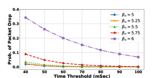
Figure 2: $\mathbb{P}_{n}^{dly}(\beta_{n})$ vs. $T^{th}_{n}$ by Different $\beta_{n}$.

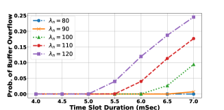
Figure 3: $\mathbb{P}_{n}^{ov}(\beta_{n})$ vs. $T^{slt}_{n}$ by Different $\lambda_{n}$.

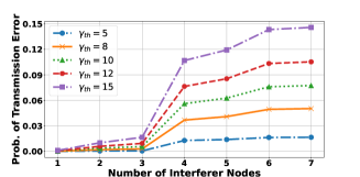
Figure 4: $\mathbb{P}_{n}^{err}(\boldsymbol{\beta})$ vs. # of Interferers by Different $\gamma_{th}$.

IV-A Queuing Analysis

IV-A1 Time Threshold Model

The source node $n\in\boldsymbol{N}$ might transmit time-sensitive packets, such as C2 packets, to UAV nodes. Hence, it is important to ensure a reliable delivery of these packets to the destination before a predetermined timeout. Let $T_{n}$ represent the waiting time in the queue for the source node. Sometimes, the source node cannot transmit the packet due to poor channel conditions, such as low SINR; any packet with a waiting time $T_{n}$ exceeding the time threshold $T_{n}^{th}$ will be discarded [34].

Let $t_{n}$ be the number of time slots necessary for the source node to transmit a packet to the destination through the channel. Using exponential distribution and $\mu_{n}(\beta_{n})$ derived from Eq. (3), the PDF of $t_{n}$ can be approximated as:

$$\begin{aligned} \mathbb{P}(t_{n}=x)&=(1-\mu_{n}(\beta_{n}))^{x-1}\mu_{n}(\beta_{n})\\ &\approx\mu_{n}(\beta_{n})e^{-\mu_{n}(\beta_{n})x}.\end{aligned}$$ (4)

Finally, the probability of dropping a packet, denoted as $\mathbb{P}_{n}^{dly}(\beta_{n})$ due to exceeding the maximum queuing delay threshold $T_{n}^{th}$ can be represented as [11]:

$$\mathbb{P}_{n}^{dly}(\beta_{n})\triangleq\mathbb{P}(T_{n}>T_{n}^{th})=e^{-(\frac{\mu_{n}(\beta_{n})}{T^{slt}_{n}}-\lambda_{n})T_{n}^{th}},$$ (5)

where $\lambda_{n}$ represents the average incoming packet rate following a Poisson distribution and $T^{slt}_{n}$ is the time slot duration. Upper Bound of Fading Threshold. The upper bound of $\beta_{n}$ for Rician distribution can be determined by $\mathbb{P}_{n}^{dly}(\beta_{n})\leq 1$, and by solving the following:

$$Q_{1}(b,\beta_{n}) \geq 1-(1-\lambda_{n}T^{slt}_{n})^{\frac{1}{|\boldsymbol{F}|}}.$$ (6)

IV-A2 Buffer Overflow Model

In addition to the time threshold model that addresses the time sensitivity of data packets, queues are assumed to have finite buffer sizes. In cases where the source node cannot transmit packets due to poor channel conditions, buffer overflow may occur. When the buffer reaches full capacity, any incoming packets will be dropped. Using the principles of queuing theory, the probability of exceeding the buffer capacity in a particular state $i$, where $i\geq 0$, is determined as [35]:

$$\overline{\mathbb{P}_{i,i+1}}=\mathbb{P}[x_{1}+...+x_{i+1}>b_{n}|x_{1}+...+x_{i}\leq b_{n}].$$ (7)

Here, $b_{n}$ denotes the buffer capacity for the source node $n\in\boldsymbol{N}$, and $x$ is the packet length following an exponential random variable with a parameter $\eta_{n}$. By applying the Markov chain, the probability of buffer overflow, which represents the probability of packet loss, can be approximated as [26]:

$$\mathbb{P}_{n}^{ov}(\beta_{n}) \approx\sum_{i=0}^{\infty}\overline{\mathbb{P}_{i,i+1}}\pi_{i}=\frac{(1-\rho_{n}(\beta_{n}))e^{-\tilde{b}_{n}(1-\rho_{n}(\beta_{n}))}}{1-\rho_{n}(\beta_{n})e^{-\tilde{b}_{n}(1-\rho_{n}(\beta_{n}))}},$$

where $\rho_{n}(\beta_{n})=\frac{\lambda_{n}T^{slt}_{n}}{\mu_{n}(\beta_{n})}$ and $\tilde{b}_{n}=b_{n}\eta_{n}$ are the offered load and normalized buffer capacity, respectively. Notably, the buffer overflow model resembles the M/M/1/K queue model by assuming $\tilde{b}_{n}=K\geq 50$. Further details and proof are provided in Appendix A.

IV-B Interference Analysis

In this section, we evaluate the impact of interference on the main channel between the source node and its destination. We aim to determine the probability of transmission error due to high interference from other nodes operating in the same spectrum band. Assuming that $\gamma_{th}$ denotes the SINR threshold, a transmission error occurs when the SINR falls below the SINR threshold $\gamma_{th}$. Let $I_{n}^{f}(\boldsymbol{\beta}_{-n})$ represent the impact of interferer nodes on the destination, which is given by [11]:

$$I_{n}^{f}(\boldsymbol{\beta}_{-n})=\sum_{m\in\boldsymbol{N}\backslash n}P_{m}(\hat{h}_{m}^{f})^{2}(\tilde{h}_{m}^{f})^{2}\alpha_{m}^{f}(\beta_{m}),$$ (8)

where $(\hat{h}_{m}^{f})^{2}$ and $(\tilde{h}_{m}^{f})^{2}$ are the path loss and the square of fading coefficient between the interferer nodes and the destination, respectively. Furthermore, $P_{m}$ and $\boldsymbol{\beta}_{-n}\triangleq(\boldsymbol{\beta}_{\boldsymbol{m}})_{\boldsymbol{m}\subset\boldsymbol{N}\backslash n}$ are the transmission power and the fading threshold of the interferer nodes. In addition, $\alpha_{m}^{f}(\beta_{m})$ equals one if interferer node $m$ transmits using channel $f$, and zero otherwise. Thus, the probability of transmission error $\mathbb{P}_{n}^{err}(\boldsymbol{\beta})$ is defined as:

$$\mathbb{P}_{n}^{err}(\boldsymbol{\beta})\triangleq\mathbb{P}(\gamma_{n}<\gamma_{th})=\mathbb{P}\Big{(}\frac{P_{n}(\hat{h}_{n}^{f})^{2}(\tilde{h}_{n}^{f})^{2}}{\sigma^{2}+I_{n}^{f}(\boldsymbol{\beta}_{-n})}<\gamma_{th}\Big{)},$$ (9)

where $P_{n}$ denotes the transmission power of the source node, and $\sigma^{2}=kTW$ represents the thermal noise power where $k$, $T$, and $W$ are the Boltzmann constant, noise temperature, and bandwidth, respectively.

By adopting a classical stochastic geometry approach, the aggregated interference $I_{n}^{f}(\boldsymbol{\beta}_{-n})$ can be modeled using Log-normal distribution, which better fits the real distribution than Gamma distribution [18]. Thus, PDF of $I_{n}^{f}(\boldsymbol{\beta}_{-n})$ is given by:

$$\zeta_{n}(x)=\mathbb{P}(I_{n}^{f}(\boldsymbol{\beta}_{-n})=x)=\frac{\text{exp}(-\frac{(\text{ln}x-\mu(\boldsymbol{\beta}_{-n}))^{2}}{2\sigma^{2}(\boldsymbol{\beta}_{-n})})}{x\sigma(\boldsymbol{\beta}_{-n})\sqrt{2\pi}},$$ (10)

where $\mu(\boldsymbol{\beta}_{-n})$ and $\sigma(\boldsymbol{\beta}_{-n})$ are the location and scale parameters in Log-normal distribution, respectively, which are derived in Appendix B. Then, the complementary cumulative distribution function (CCDF) of $I_{n}^{f}(\boldsymbol{\beta}_{-n})$ can be expressed as:

$$v_{n}(x,\boldsymbol{\beta}_{-n})\triangleq\mathbb{P}(x<I_{n}^{f}(\boldsymbol{\beta}_{-n}))=\frac{1}{2}-$$ (11)

$$\frac{1}{2}\text{erf}(\frac{\ln(x)-\mu(\boldsymbol{\beta}_{-n})}{\sqrt{2}\sigma(\boldsymbol{\beta}_{-n})})=1-\phi(\frac{\ln(x)-\mu(\boldsymbol{\beta}_{-n})}{\sigma(\boldsymbol{\beta}_{-n})}).$$

Here, $\text{erf}(x)=\frac{2}{\sqrt{\pi}}\int_{0}^{x}e^{-t^{2}}dt$ is the error function and $\phi(x)$ denotes the CDF of the standard normal distribution. Eventually, $\mathbb{P}_{n}^{err}(\boldsymbol{\beta})$ using Eq. (9) can be defined as [11, 18]:

$$\mathbb{P}_{n}^{err}(\boldsymbol{\beta}) =\mathbb{P}\Big{(}\frac{P_{n}(\hat{h}_{n}^{f})^{2}(\tilde{h}_{n}^{f})^{2}}{\gamma_{th}}-\sigma^{2}<I_{n}^{f}(\boldsymbol{\beta}_{-n})\Big{)}$$

$$=\int_{\beta_{n}}^{\infty}\mathbb{P}(\tilde{h}_{n}^{f}=x)v_{n}\Big{(}\frac{P_{n}(\hat{h}_{n}^{f})^{2}}{\gamma_{th}}x^{2}-\sigma^{2},\boldsymbol{\beta}_{-n}\Big{)}dx,$$

where $\mathbb{P}(\tilde{h}_{n}^{f}=x)$ represents the PDF of Rician or Rayleigh distributions between the source node and its destination.

IV-C Distributed Throughput Optimization

In the queuing and interference analysis sections, we calculated the probability of time threshold $\mathbb{P}_{n}^{dly}(\beta_{n})$ due to exceeding the maximum queuing delay, the probability of buffer overflow $\mathbb{P}_{n}^{ov}(\beta_{n})$ due to full buffer capacity, and the probability of transmission error $\mathbb{P}_{n}^{err}(\boldsymbol{\beta})$ caused by SINR falling below the SINR threshold where the behavior of them with respect to different parameters are shown in Figs. 4, 4 and 4, respectively. Due to the negligible product of $\mathbb{P}_{n}^{dly}(\beta_{n})$, $\mathbb{P}_{n}^{ov}(\beta_{n})$ and $\mathbb{P}_{n}^{err}(\boldsymbol{\beta})$, the probability of overall loss $\mathbb{P}_{n}^{lss}(\boldsymbol{\beta})$ can be approximated by:

$$\small\begin{aligned} \mathbb{P}_{n}^{lss}(\boldsymbol{\beta})&=\mathbb{P}_{n}^{ov}(\beta_{n})+[1-\mathbb{P}_{n}^{ov}(\beta_{n})]\mathbb{P}_{n}^{dly}(\beta_{n})+[1-\mathbb{P}_{n}^{ov}(\beta_{n})]\times\\ &[1-\mathbb{P}_{n}^{dly}(\beta_{n})]\mathbb{P}_{n}^{err}(\boldsymbol{\beta})\approx\mathbb{P}_{n}^{ov}(\beta_{n})+\mathbb{P}_{n}^{dly}(\beta_{n})+\mathbb{P}_{n}^{err}(\boldsymbol{\beta}).\end{aligned}$$

Given the probability of overall loss $\mathbb{P}_{n}^{lss}(\boldsymbol{\beta})$, the throughput $\mathbb{R}_{n}(\boldsymbol{\beta})$ is approximated as:

$$\begin{aligned} \mathbb{R}_{n}(\boldsymbol{\beta})&=\lambda_{n}[1-\mathbb{P}_{n}^{lss}(\boldsymbol{\beta})]\\ &\approx\lambda_{n}[1-\mathbb{P}_{n}^{dly}(\beta_{n})-\mathbb{P}_{n}^{ov}(\beta_{n})-\mathbb{P}_{n}^{err}(\boldsymbol{\beta})],\end{aligned}$$ (12)

Theorem 1.

Given the provided expressions, $\mathbb{R}_{n}(\boldsymbol{\beta})$ is a concave function with respect to $\beta_{n}$.

Proof.

The proof is provided in Appendix C. ∎

With this theorem, we aim to develop a distributed algorithm by which different nodes adjust their fading thresholds $\beta_{i}$ to maximize the throughput. In this case, distributed nodes should coordinate to converge to the optimal fading threshold or transmission policy, which is advantageous for all nodes. To solve this problem, we use consensus-based distributed optimization, which tries to reach a consensus on the fading threshold $\boldsymbol{\beta}$ as different nodes collaborate [36]. Our proposed Distributed Transmission Control (DTC) policy is presented in Algorithm 1 by which we maximize the throughput by finding the optimal fading threshold $\boldsymbol{\beta}^{\star}$.

Algorithm 1 Distributed Transmission Control (DTC)

1:function DTC($\hat{\boldsymbol{m}}$, $\boldsymbol{stp}$, $itr$, $\boldsymbol{\beta}^{max}$)

2:    $\boldsymbol{m}^{prv}\leftarrow\hat{\boldsymbol{m}}$, $\boldsymbol{\beta}\leftarrow\boldsymbol{\beta}^{max}$

3:    for $n$ in range $\hat{\boldsymbol{m}}$ do

4:         $bst\leftarrow\mathbb{R}_{n}(\boldsymbol{\beta})$, $\beta_{n}\leftarrow\boldsymbol{\beta}[n]$, $\boldsymbol{m}\leftarrow\hat{\boldsymbol{m}}-\{n\}$

5:         $\boldsymbol{\beta}^{slf}[n]\leftarrow\text{LCS}(\boldsymbol{0},\boldsymbol{\beta},\boldsymbol{stp},bst,\boldsymbol{\beta}^{max},0)$

6:         $\hat{\boldsymbol{m}}\leftarrow\boldsymbol{m}^{prv}$

7:    end for

8:    $\boldsymbol{\beta}^{\star}\leftarrow\boldsymbol{\beta}^{slf}$

9:    for $i$ in range $itr$ do $\boldsymbol{\beta}\leftarrow\boldsymbol{\beta}^{\star}$

10:         for $n$ in range $\hat{\boldsymbol{m}}$ do

11:             $\beta_{n}\leftarrow\boldsymbol{\beta}[n]$, $\boldsymbol{m}\leftarrow\hat{\boldsymbol{m}}-\{n\}$

12:             $bst\leftarrow\textbf{R}[i][n]\leftarrow\mathbb{R}_{n}(\boldsymbol{\beta})$

13:             $\boldsymbol{\beta}^{\star}[n]\leftarrow\text{LCS}(\boldsymbol{0},\boldsymbol{\beta},\boldsymbol{stp},bst,\boldsymbol{\beta}^{max},0)$

14:             $\hat{\boldsymbol{m}}\leftarrow\boldsymbol{m}^{prv}$

15:         end for

16:         if $|\boldsymbol{\beta}-\boldsymbol{\beta}^{\star}|<\epsilon$ then

17:             break

18:         end if

19:    end for

20:    return $\boldsymbol{\beta}^{\star}$

21:end function

Initially, this algorithm sets the fading threshold $\boldsymbol{\beta}$ to the maximum value $\boldsymbol{\beta}^{max}$, which is obtained from the upper bound of the fading threshold. The algorithm then finds the selfish fading threshold $\boldsymbol{\beta}^{slf}$ for all nodes, where each node assumes that the other nodes are not transmitting. Then, it starts to discover the optimal fading threshold $\boldsymbol{\beta}^{\star}$ by the initialized selfish values. To do this, the DTC algorithm utilizes the Local Coordinate Search (LCS) function presented in Appendix E to determine the maximum throughput and associated best fading threshold for each node in each iteration. In the end, if the difference in the fading thresholds for two consecutive iterations is less than $\epsilon$, this algorithm returns the optimal fading threshold $\boldsymbol{\beta}^{\star}$. At each iteration, the calculated throughput $\mathbb{R}_{n}(\boldsymbol{\beta})$ will be stored in the throughput set R, where the first dimension denotes the index of iterations and the second dimension represents the index of the nodes. In the next section, we extend this analysis to incorporate video transmission control policies.

V Joint Distributed Video Transmission and Encoder Control

In the previous section, we presented the DTC algorithm, which aims to maximize performance through distributed transmission control. In this section, we further extend our setup by incorporating video encoding rate optimization. Therefore, the performance metric is expanded from focusing solely on throughput optimization to include PSNR optimization, which accounts for video distortion.

V-A Video Distortion and PSNR Analysis

Given the probability of overall loss $\mathbb{P}_{n}^{lss}(\boldsymbol{\beta})$, we define the packet loss distortion as $\mathrm{D}_{n}^{lss}(\boldsymbol{\beta})=s_{n}\mathbb{P}_{n}^{lss}(\boldsymbol{\beta})$, where $s_{n}$ is the sensitivity parameter of a video sequence to packet loss. Moreover, we assume $\mathrm{D}_{n}^{cmp}(\mathrm{E}_{n})=D_{0}+\frac{\theta_{0}}{\mathrm{E}_{n}-E_{0}}$ represents the lossy video compression distortion. Here, $\mathrm{E}_{n}=\lambda_{n}L_{n}$ denotes the video encoding rate at the application layer, where $L_{n}$ is the average video packet length. Also, $D_{0}$, $\theta_{0}$, and $E_{0}$ are the parameters of video rate-distortion model, which can be determined using nonlinear regression techniques [34]. According to the packet loss distortion $\mathrm{D}_{n}^{lss}(\boldsymbol{\beta})$ and the lossy video compression distortion $\mathrm{D}_{n}^{cmp}(\mathrm{E}_{n})$, the overall video distortion $\mathrm{D}_{n}(\mathrm{E}_{n},\boldsymbol{\beta})$ is given by [18]:

$$\begin{aligned} \mathrm{D}_{n}(\mathrm{E}_{n},\boldsymbol{\beta})&=\mathrm{D}_{n}^{cmp}(\mathrm{E}_{n})+\mathrm{D}_{n}^{lss}(\boldsymbol{\beta})\\ &=D_{0}+\frac{\theta_{0}}{\mathrm{E}_{n}-E_{0}}+s_{n}\mathbb{P}_{n}^{lss}(\boldsymbol{\beta}).\end{aligned}$$ (13)

Given the overall video distortion, we calculate the PSNR, an important metric for video transmission quality measurement. The PSNR metric is defined by the widely used mean square error rate-distortion model. Therefore, given the overall video distortion $\mathrm{D}_{n}(\mathrm{E}_{n},\boldsymbol{\beta})$, PSNR between the source node $n\in\boldsymbol{N}$ and its destination is calculated as [18, 37]:

$$\mathcal{P}_{n}(\mathrm{E}_{n},\boldsymbol{\beta})=10\log_{10}\Big{(}\frac{(2^{p}-1)^{2}}{\mathrm{D}_{n}(\mathrm{E}_{n},\boldsymbol{\beta})}\Big{)},$$ (14)

where $p$ is the bit-depth of a video pixel. In Eq. (14), the encoding rate $\mathrm{E}_{n}$ and fading threshold $\boldsymbol{\beta}$ are jointly incorporated into our cross-layer formulation including packet loss distortion $\mathrm{D}_{n}^{lss}(\boldsymbol{\beta})$ at the PHY and MAC layers and lossy video compression distortion $\mathrm{D}_{n}^{cmp}(\mathrm{E}_{n})$ at the application layer.

Algorithm 2 Joint Distributed Video Transmission and Encoder Control (JDVT-EC)

1:function JDVT-EC($\boldsymbol{\mathrm{E}}^{ini}$, $\boldsymbol{\beta}^{ini}$, $\hat{\boldsymbol{m}}$, $\boldsymbol{stp}$, $itr$, $\boldsymbol{\beta}^{max}$)

2:    $\boldsymbol{\mathrm{E}}^{\star}\leftarrow\boldsymbol{\mathrm{E}}^{ini}$, $\boldsymbol{\beta}^{\star}\leftarrow\boldsymbol{\beta}^{ini}$

3:    for $ctr$ in range $itr$ do $\boldsymbol{\mathrm{E}}^{prv}\leftarrow\boldsymbol{\mathrm{E}}^{\star}$, $\boldsymbol{\beta}^{prv}\leftarrow\boldsymbol{\beta}^{\star}$

4:         $\boldsymbol{\beta}^{\star}\leftarrow\text{DVTC}(\boldsymbol{\mathrm{E}}^{\star},\boldsymbol{\beta}^{\star},\hat{\boldsymbol{m}},\boldsymbol{stp},itr,ctr,\boldsymbol{\beta}^{max})$

5:         $\boldsymbol{\mathrm{E}}^{\star}\leftarrow\text{DVEC}(\boldsymbol{\mathrm{E}}^{\star},\boldsymbol{\beta}^{\star},\hat{\boldsymbol{m}},\boldsymbol{stp},ctr)$

6:         if $|\boldsymbol{\beta}^{prv}-\boldsymbol{\beta}^{\star}|<\epsilon$ and $|\boldsymbol{\mathrm{E}}^{prv}-\boldsymbol{\mathrm{E}}^{\star}|<\epsilon$ then

7:             break

8:         end if

9:    end for

10:    return $\boldsymbol{\mathrm{E}}^{\star}$, $\boldsymbol{\beta}^{\star}$

11:end function

To characterize the PSNR in a 3D space, we define the average PSNR ($\bar{\mathcal{P}}_{n}$) between the source node and its destination as the mean PSNR value calculated over discretized distances and elevation angles, as follows [14]:

$$\bar{\mathcal{P}}_{n}=\frac{1}{|\textbf{d}||\Theta|}\sum_{j=\theta_{n}^{min}}^{\theta_{n}^{max}}\sum_{i=d_{n}^{min}}^{d_{n}^{max}}\mathcal{P}^{ij}_{n}(\mathrm{E}_{n},\boldsymbol{\beta}),$$ (15)

where $d_{n}^{min}$ and $d_{n}^{max}$ are the minimum and maximum distances, which can be included in a discrete distance set d = {$d_{n}^{min},...,d_{n}^{max}$}. Similarly, $\theta_{n}=\arctan{(\frac{d_{n}^{V}}{d_{n}^{H}})}$ denotes the elevation angle where $\theta_{n}^{min}$ and $\theta_{n}^{max}$ are the minimum and maximum elevation angles given in a discrete elevation angle set $\Theta$ = {$\theta_{n}^{min},...,\theta_{n}^{max}$}.

Theorem 2.

Given the expressions provided for PSNR in Eq. (14), $\mathcal{P}_{n}(\mathrm{E}_{n},\boldsymbol{\beta})$ is concave with respect to $E_{n}$ and $\beta_{n}$.

Proof.

The proofs are provided in Appendices D and C. ∎

Based on this result, next we propose a distributed algorithm to maximize the PSNR values.

V-B Distributed PSNR Optimization

The goal is to maximize the average PSNR for streamer nodes in the environment. To do this, two important parameters, including the encoding rate $\mathrm{E}_{n}$ and the fading threshold $\beta_{n}$, need to be optimized for each node. Therefore, the optimization problem is divided into two sub-problems to solve each parameter individually. To solve the distributed PSNR optimization, we propose Joint Distributed Video Transmission and Encoder Control (JDVT-EC), as described in Algorithm 2. In each iteration, the JDVT-EC optimization algorithm finds the optimal fading threshold $\boldsymbol{\beta}^{\star}$ and the optimal encoding rate $\boldsymbol{\mathrm{E}}^{\star}$ using the DVTC and DVEC sub-algorithms and compares it with the previous fading threshold $\boldsymbol{\beta}^{prv}$ and the previous encoding rate $\boldsymbol{\mathrm{E}}^{prv}$. Finally, if the difference between the optimal and previous sets is smaller than $\epsilon$, the algorithm returns the optimal fading threshold $\boldsymbol{\beta}^{\star}$ and the optimal encoding rate $\boldsymbol{\mathrm{E}}^{\star}$. In this algorithm, $ctr$ counts the number of iterations, and $itr$ specifies the maximum number of iterations.

Algorithm 3 Distributed Video Transmission Control (DVTC)

1:function DVTC($\boldsymbol{\mathrm{E}}^{\star}$, $\boldsymbol{\beta}^{\star}$, $\hat{\boldsymbol{m}}$, $\boldsymbol{stp}$, $itr$, $ctr$, $\boldsymbol{\beta}^{max}$)

2:    $\boldsymbol{m}^{prv}\leftarrow\hat{\boldsymbol{m}}$

3:    for $i$ in range $itr$ do $\boldsymbol{\beta}\leftarrow\boldsymbol{\beta}^{\star}$

4:         for $n$ in range $\hat{\boldsymbol{m}}$ do

5:             $\mathrm{E}_{n}\leftarrow\boldsymbol{\mathrm{E}}^{\star}[n]$, $\beta_{n}\leftarrow\boldsymbol{\beta}[n]$, $\boldsymbol{m}\leftarrow\hat{\boldsymbol{m}}-\{n\}$

6:             $bst\leftarrow\boldsymbol{\mathcal{P}}[2ctr][i][n]\leftarrow\mathcal{P}_{n}(\mathrm{E}_{n},\boldsymbol{\beta})$

7:             $\boldsymbol{\beta}^{\star}[n]\leftarrow\text{LCS}(\mathrm{E}_{n},\boldsymbol{\beta},\boldsymbol{stp},bst,\boldsymbol{\beta}^{max},0)$

8:             $\hat{\boldsymbol{m}}\leftarrow\boldsymbol{m}^{prv}$

9:         end for

10:         if $|\boldsymbol{\beta}-\boldsymbol{\beta}^{\star}|<\epsilon$ then

11:             break

12:         end if

13:    end for

14:    return $\boldsymbol{\beta}^{\star}$

15:end function

Algorithm 4 Distributed Video Encoder Control (DVEC)

1:function DVEC($\boldsymbol{\mathrm{E}}^{\star}$, $\boldsymbol{\beta}^{\star}$, $\hat{\boldsymbol{m}}$, $\boldsymbol{stp}$, $ctr$)

2:    $\boldsymbol{m}^{prv}\leftarrow\hat{\boldsymbol{m}}$, $\boldsymbol{\beta}\leftarrow\boldsymbol{\beta}^{\star}$

3:    for $n$ in range $\hat{\boldsymbol{m}}$ do

4:         $\mathrm{E}_{n}\leftarrow\boldsymbol{\mathrm{E}}^{\star}[n]$, $\beta_{n}\leftarrow\boldsymbol{\beta}[n]$, $\boldsymbol{m}\leftarrow\hat{\boldsymbol{m}}-\{n\}$

5:         $bst\leftarrow\boldsymbol{\mathcal{P}}[2ctr+1][0][n]\leftarrow\mathcal{P}_{n}(\mathrm{E}_{n},\boldsymbol{\beta})$

6:         $\boldsymbol{\mathrm{E}}^{\star}[n]\leftarrow\text{LCS}(\mathrm{E}_{n},\boldsymbol{\beta},\boldsymbol{stp},bst,\boldsymbol{0},1)$

7:         $\hat{\boldsymbol{m}}\leftarrow\boldsymbol{m}^{prv}$

8:    end for

9:    return $\boldsymbol{\mathrm{E}}^{\star}$

10:end function

In the Distributed Video Transmission Control (DVTC) algorithm, like the DTC algorithm, ground/aerial nodes collaborate to achieve an optimal distributed transmission strategy that is beneficial to all nodes, assuming that each link can be a main link. Accordingly, multiple nodes coordinate to achieve a consensus on the fading threshold set $\boldsymbol{\beta}$ while keeping the encoding rate constant [36]. Each node contains its local information, iteratively communicating with adjacent nodes to determine the optimal fading threshold $\boldsymbol{\beta}^{\star}$. Algorithm 3 presents the DVTC policy to determine the optimal fading threshold set $\boldsymbol{\beta}^{\star}$ for all nodes. In each iteration, if the difference between the updated fading threshold set $\boldsymbol{\beta}^{\star}$ and the preceding one $\boldsymbol{\beta}$ exceeds $\epsilon$, nodes share information about their fading thresholds with each other to specify the optimal fading threshold again. In this algorithm, $n$ and set $\boldsymbol{m}$ denote the source node and interferer nodes while set $\hat{\boldsymbol{m}}$ contains both the source node and interferer nodes. Also, $\boldsymbol{stp}$ set denotes the step parameters, which are used in the LCS function, and $\boldsymbol{\beta}^{max}$ set represents the maximum value of the fading thresholds corresponding to the upper bounds. Moreover, the LCS function computes the best fading threshold $\beta_{n}$ for each node while having access to $\boldsymbol{\beta}_{m}$, which explores coordinates by step parameters until it identifies the best fading threshold $\beta_{n}$ associated with the maximum PSNR $\mathcal{P}_{n}$ [38]. In each iteration, the computed PSNR $\mathcal{P}_{n}$ will be stored in the 3-dimensional $\boldsymbol{\mathcal{P}}$ set, in which the $1^{st}$, $2^{nd}$, and $3^{rd}$ dimensions are related to JDVT-EC algorithm counter, iteration number in the specific algorithm, and the source node index, respectively.

TABLE I: Key Simulation Parameters

Definition	Notation & Value
Communication Area	$100\times 100\,\text{m}^{2}$
Environmental Parameters	$\zeta=20$, $v=3\times 10^{-4}$, $\mu=0.5$
Path Loss Exponent	$\alpha_{L}=2$, $\alpha_{N}=3.5$
Reference Distance	$d_{0}=10$ m
Number of Sub-Channels	$|\boldsymbol{F}|=14$
Rician Factor	$K_{L}=15$, $K_{N}=1$
Time Threshold	$T^{th}_{n}=80$ ms
Time Slot Duration	$T^{slt}_{n}=5$ ms
Normalized Buffer Capacity	$\tilde{b}_{n}=100$
Transmission Power	$P_{n}=0.2$ W
SINR Threshold	$\gamma_{th}=10$
Operating Frequency	$f=2.4$ GHz
Noise Temperature	$T=290$ K
Bandwidth	$W=100$ MHz
Boltzmann Constant	$k=1.38\times 10^{-23}$ J/K
Sensitivity Parameter	$s_{n}=30$
Average Video Packet Length	$L_{n}=3.04$ Kb
Rate-Distortion Parameters	$D_{0}=1.18$, $E_{0}=0.67$, $\theta_{0}=858$
Video Pixel Bit-Depth	$p=8$
Fading Threshold Step	$\boldsymbol{stp}_{\beta}=\{0.5,0.01\}$
Incoming Packet Rate Step	$\boldsymbol{stp}_{\lambda}=\{0.5,1\}$

TABLE II: Fading Threshold $\beta_{i}$ for Different Policies

Policy	Streamer UAV	Interferer UAV	Node 3	Node 4	Node 5	Node 6	Node 7	Node 8	Node 9	Node 10
Random	3.16	3.53	3.01	1.48	2.54	1.56	2.49	1.57	4.06	4.08
Aggressive	3.18	3.35	2.03	2.03	1.44	1.88	1.79	1.46	3.43	4.16
Selfish	5.06	5.35	2.73	2.97	2.39	2.97	2.85	2.95	5.76	5.14
Fixed	4.00	4.00	2.00	2.00	2.00	2.00	2.00	2.00	4.00	4.00
Optimal	5.12	5.44	2.82	2.98	2.57	2.98	2.93	2.97	5.78	5.17
Conservative	5.33	5.94	2.93	3.06	2.95	3.07	3.20	3.04	6.07	5.36

To solve the second sub-problem, the Distributed Video Encoder Control (DVEC) method, as described in Algorithm 4 aims to find the optimal encoding rate set $\boldsymbol{\mathrm{E}}^{\star}$ for streamer nodes using the LCS algorithm. Unlike the DVTC algorithm, each source node’s video encoding rate $\mathrm{E}_{n}$ does not impact other nodes’ video encoding rates. Therefore, $\boldsymbol{\mathrm{E}}^{\star}$ does not need to be solved iteratively. In this algorithm, each node in $\hat{\boldsymbol{m}}$ can be a source node $n\in\boldsymbol{N}$, which can find the optimal video encoding rate $\mathrm{E}_{n}^{\star}$ and store it in the optimal encoding rate set $\boldsymbol{\mathrm{E}}^{\star}$ without changing $\boldsymbol{\beta}$. Finally, the algorithm returns the optimal encoding rates $\boldsymbol{\mathrm{E}}^{\star}$ for the JDVT-EC algorithm.

VI Evaluation Results

To evaluate the performance of the proposed algorithms, we consider a network in which $10$ ground/aerial nodes are placed according to the Poisson distribution in the environment. The network includes $1$ streamer UAV (node index 1), $1$ interferer UAV (node index $2$), and $8$ ground nodes (nodes indices $3$ to $10$). In this case, $2$ ground nodes (nodes $10$ and $9$) are, respectively, paired with the streamer and interferer UAVs, and the other $6$ ground nodes (nodes $3$ to $8$) establish $3$ G2G pairs. We assume that the streamer and interferer UAVs are streaming videos to their associated ground nodes in the downlink, also 3 ground nodes are streaming to their paired ground nodes. On the other hand, 3 G2G pairs and 2 G2A pairs transmit short packets (e.g., C2 messages). The key simulation parameters are summarized in Table I.

VI-A Throughput Optimization Performance

VI-A1 DTC Algorithm Performance

TABLE III: $R_{i}^{\star}-\beta_{i}^{\star}$ Values by DTC Algorithm

$\gamma_{th}$	Streamer UAV	Interferer UAV	Node 3	Node 4	Node 5	Node 6	Node 7	Node 8	Node 9	Node 10
5	96.60 - 5.08	99.87 - 5.26	98.88 - 2.77	88.94 - 2.98	99.90 - 2.45	89.46 - 2.97	95.87 - 2.90	90.65 - 2.96	94.40 - 5.73	93.38 - 5.14
8	95.01 - 5.11	99.72 - 5.39	98.39 - 2.81	88.93 - 2.98	99.84 - 2.54	89.17 - 2.98	94.82 - 2.92	89.98 - 2.97	91.27 - 5.77	91.33 - 5.16
10	94.20 - 5.12	99.60 - 5.44	98.08 - 2.82	88.92 - 2.98	99.80 - 2.57	89.09 - 2.98	94.25 - 2.93	89.73 - 2.97	90.24 - 5.78	90.60 - 5.17
12	93.58 - 5.13	99.47 - 5.48	97.81 - 2.84	88.92 - 2.98	99.75 - 2.61	89.04 - 2.98	93.88 - 2.93	89.57 - 2.97	89.68 - 5.78	90.14 - 5.17
15	92.81 - 5.14	99.25 - 5.52	97.44 - 2.85	88.92 - 2.98	99.67 - 2.64	88.99 - 2.98	93.33 - 2.94	89.40 - 2.97	89.27 - 5.78	89.69 - 5.17

$|\boldsymbol{F}|$	Streamer UAV	Interferer UAV	Node 3	Node 4	Node 5	Node 6	Node 7	Node 8	Node 9	Node 10
8	85.42 - 4.90	97.64 - 5.32	94.20 - 2.62	82.77 - 2.72	99.03 - 2.45	82.79 - 2.72	86.95 - 2.70	82.92 - 2.72	82.84 - 5.52	83.44 - 4.91
11	90.99 - 5.03	99.15 - 5.40	96.85 - 2.74	86.58 - 2.87	99.61 - 2.53	86.64 - 2.87	91.65 - 2.83	87.01 - 2.86	87.07 - 5.67	87.78 - 5.06
14	94.20 - 5.12	99.60 - 5.44	98.08 - 2.82	88.92 - 2.98	99.80 - 2.57	89.09 - 2.98	94.25 - 2.93	89.73 - 2.97	90.24 - 5.78	90.60 - 5.17
17	96.11 - 5.19	99.78 - 5.47	98.73 - 2.89	90.53 - 3.06	99.87 - 2.61	90.83 - 3.06	95.89 - 3.00	91.67 - 3.05	92.75 - 5.85	92.64 - 5.25
20	97.25 - 5.24	99.86 - 5.50	99.11 - 2.93	91.71 - 3.13	99.91 - 2.64	92.12 - 3.13	96.87 - 3.05	93.13 - 3.11	94.65 - 5.91	94.22 - 5.31

Fig. 5 demonstrates the distribution of nodes in the 100$\times$100 $\text{m}^{2}$ area in which the star symbol marks the streamer and interferer UAVs at the altitudes of $50$ m and $60$ m, respectively; also, the circles denotes the ground nodes. Double arrow lines display the main links between the nodes; the solid ones are the G2A or A2G LoS channels, and the dashed ones are the G2G NLoS channels. Using the heatmap, the optimal throughput $R_{i}^{\star}$ obtained by the DTC algorithm is shown as source nodes transmit their packets to destination nodes. The results show that the destination nodes further away from the “crowded area” (such as nodes $6$, $8$, and $9$) experience a better throughput after reaching a consensus on the fading threshold $\beta_{i}$. However, the streamer and interferer UAVs suffer from A2A interference, resulting in a lower throughput than G2G communications pairs.

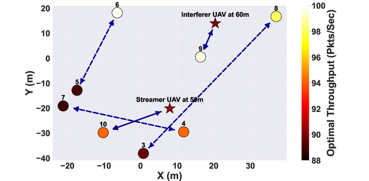
Figure 5: Nodes Distribution vs. $R_{i}^{\star}$ by DTC Algorithm.

In Table II, we compare the DTC algorithm performance with $5$ baselines to set the fading thresholds $\beta_{i}$, which are defined as: (1) Random Policy: Nodes set the fading threshold $\beta_{i}$ randomly between zero and the upper bound. (2) Aggressive Policy: Nodes set the fading threshold $\beta_{i}$ to low values to send their packets even under bad channel conditions and enqueue fewer packets. Thus, nodes experience more packet losses due to the channel conditions. (3) Selfish Policy: Nodes set the fading threshold $\beta_{i}$ selfishly by assuming that the fading threshold of other nodes is equal to the upper bound (lines 3-7 in the DTC algorithm). Thus, nodes do not collaborate to find the optimal fading threshold $\beta_{i}^{\star}$ by consensus. (4) Fixed Policy: Nodes set the fading threshold $\beta_{i}$ as a fixed value, which is assumed to be $\beta_{i}=4$ for LoS channels and $\beta_{i}=2$ for NLoS channels. (5) Conservative Policy: Nodes set the fading threshold $\beta_{i}$ close to the upper bound, so they enqueue more packets instead of transmitting them over the channel. Therefore, nodes experience less packet loss in the channel, but more in the queue. From the results in Table II, we observe that the DTC algorithm finds the optimal fading threshold $\beta_{i}^{\star}$ that is smaller than the conservative policy, but larger than the aggressive policy for all nodes since the algorithm balances the trade-offs between different packet loss probabilities. In addition, the optimal fading threshold $\beta_{i}^{\star}$ is slightly higher than the selfish policy since each node increases its fading threshold during collaboration to improve overall system performance. Similarly, Fig. 6 compares optimal throughput $R_{i}^{\star}$ with the above baselines, as well as the “no-interference” scenario. The results show that the DTC algorithm outperforms all $5$ policies while achieving a close performance to the no-interference scenario, which denotes the maximum achievable throughput $R_{i}$ in the environment. Thus, our proposed DTC algorithm balances the trade-off between packet loss due to poor channel condition (i.e., smaller $\beta_{i}$) vs. packet loss due to buffer overflow and time threshold model (i.e., larger $\beta_{i}$).

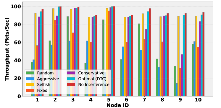
Figure 6: $R_{i}$ vs. Different Transmission Policies

TABLE IV: $\mathcal{P}_{i}-\beta_{i}-E_{i}$ Comparison for Individual or Joint Optimized Parameters

Optimized	Streamer UAV	Interferer UAV	Node 3	Node 4	Node 5	Average $\mathcal{P}^{\star}$
$E_{i}^{\star}$	39.40 - 5.00 - 346.56	42.12 - 5.00 - 413.44	38.68 - 2.00 - 422.56	36.31 - 2.00 - 431.68	41.71 - 2.00 - 416.48	39.64 dB
$\beta_{i}^{\star}$	40.53 - 5.12 - 304.00	41.97 - 5.44 - 304.00	41.52 - 2.82 - 304.00	39.47 - 2.98 - 304.00	42.03 - 2.57 - 304.00	41.10 dB
$\beta_{i}^{\star},E_{i}^{\star}$	40.37 - 5.12 - 310.08	42.51 - 5.14 - 407.36	41.70 - 2.67 - 373.92	39.50 - 3.02 - 279.68	42.62 - 2.29 - 410.40	41.34 dB

TABLE V: $\mathcal{P}_{i}-E_{i}$ Values for Different Encoding Rates

Encoding Rate	Streamer UAV	Interferer UAV	Node 3	Node 4	Node 5	Average $\mathcal{P}$
Low	38.93 - 158.08	40.67 - 203.68	38.90 - 179.36	38.92 - 191.52	40.05 - 167.20	39.49 dB
Medium	40.35 - 325.28	41.86 - 297.92	41.42 - 307.04	39.11 - 331.36	41.68 - 273.60	40.88 dB
Optimal	40.37 - 310.08	42.51 - 407.36	41.70 - 373.92	39.50 - 279.68	42.62 - 410.40	41.34 dB
High	37.00 - 431.68	42.34 - 443.84	41.30 - 425.60	35.66 - 407.36	42.42 - 449.92	39.74 dB

VI-A2 DTC Algorithm Behavior

Table III shows the optimal throughput $R_{i}^{\star}$ with different SINR thresholds $\gamma_{th}$ for all nodes. By increasing the SINR threshold $\gamma_{th}$, the optimal throughput $R_{i}^{\star}$ decreases since packets cannot be decoded at the destination with low SINR. Moreover, the optimal fading thresholds $\beta_{i}^{\star}$ are expressed as a function of different SINR thresholds $\gamma_{th}$. As the SINR threshold $\gamma_{th}$ increases, all nodes increase their optimal fading thresholds $\beta_{i}^{\star}$ generated by the DTC algorithm since the destination node cannot decode the packets and the source node would prefer to enqueue more packets instead of transmitting to the destination. As mentioned, nodes 3 to 8 establish G2G channels, so their fading threshold ranges are lower than the G2A or A2G channels. Table III also reports the optimal throughput $R_{i}^{\star}$ as the number of sub-channels $|\boldsymbol{F}|$ changes. Increasing the number of sub-channels $|\boldsymbol{F}|$ increases the optimal throughput $R_{i}^{\star}$ as the nodes have more sub-channels available to select. Furthermore, the optimal fading threshold $\beta_{i}^{\star}$ is demonstrated as the number of sub-channels $|\boldsymbol{F}|$ changes. As the number of sub-channels $|\boldsymbol{F}|$ increases, the optimal fading threshold $\beta_{i}^{\star}$ increases. This is due to the fact that the upper bound (feasible range) of the fading threshold increases by increasing the number of sub-channels $|\boldsymbol{F}|$.

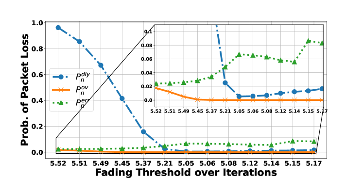
Figure 7: Probability of Packet Loss vs. $\beta_{n}$ for Node 10

In Fig. 7, the probability of packet loss including $\mathbb{P}_{n}^{dly}$, $\mathbb{P}_{n}^{ov}$ and $\mathbb{P}_{n}^{err}$ are represented for different fading thresholds $\beta_{n}$ (last one is the optimal fading threshold $\beta_{n}^{\star}$) when node 10 hits the higher throughput as the DTC algorithm iterates. At the beginning of iterations, node 10 experiences a huge packet loss due to the time threshold $\mathbb{P}_{n}^{dly}$, and the fading threshold $\beta_{n}$ is closer to the upper bound. As shown in the zoomed-in view, when the fading threshold $\beta_{n}$ decreases, packet losses in the queue and channel decrease and increase, respectively. However, there are some anomaly points, such as $\beta_{n}=5.14$, when node $10$ communicates with other nodes and receives the optimal fading threshold set $\boldsymbol{\beta}^{\star}$.

VI-B PSNR Optimization Performance

VI-B1 JDVT-EC Algorithm Performance

TABLE VI: $\beta_{i}^{\star}-E_{i}^{\star}$ Values by JDVT-EC Algorithm

Node	$s_{n}$ = 20	$s_{n}$ = 30	$s_{n}$ = 40	$s_{n}$ = 50	$s_{n}$ = 60	$\gamma_{th}$ = 5	$\gamma_{th}$ = 8	$\gamma_{th}$ = 10	$\gamma_{th}$ = 12	$\gamma_{th}$ = 15
1	5.07-337.44	5.12-310.08	5.16-288.80	5.19-273.60	5.21-261.44	5.03-334.40	5.10-316.16	5.12-310.08	5.14-304.00	5.16-297.92
2	5.10-422.56	5.14-407.36	5.17-395.20	5.20-386.08	5.21-380.00	4.92-413.44	5.07-410.40	5.14-407.36	5.19-404.32	5.26-398.24
3	2.62-395.20	2.67-373.92	2.72-352.64	2.74-343.52	2.77-328.32	2.62-380.00	2.64-376.96	2.67-373.92	2.70-367.84	2.73-361.76
4	2.97-310.08	3.02-279.68	3.06-258.40	3.10-237.12	3.13-221.92	3.02-279.68	3.02-279.68	3.02-279.68	3.02-279.68	3.02-279.68
5	2.26-425.60	2.29-410.40	2.31-401.28	2.34-392.16	2.35-386.08	2.08-413.44	2.26-410.40	2.29-410.40	2.32-410.40	2.37-407.36

Fig. 8 depicts the distribution of all nodes in the environment. The results show the optimal PSNR $\mathcal{P}_{i}^{\star}$ obtained from the JDVT-EC algorithm for each streamer node. As mentioned, the dashed and solid arrow lines are the main NLoS and LoS links, respectively. In addition, streamer nodes (nodes 1 to 5) are shown by black circles and stars in the environment. It can be seen that nodes 7 and 10 experience a lower optimal PSNR $\mathcal{P}_{i}^{\star}$ due to being in a “crowded area” with high interference.

Figure 8: Nodes Distribution vs. $\mathcal{P}_{i}^{\star}$ by JDVT-EC

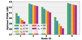
Figure 9: $\mathcal{P}_{i}^{\star}$ vs. $s_{n}$ by JDVT-EC

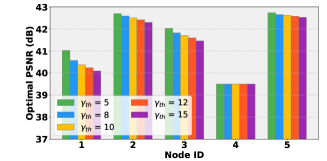
Figure 10: $\mathcal{P}_{i}^{\star}$ vs. $\gamma_{th}$ by JDVT-EC

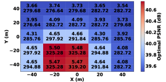
Figure 11: $\mathcal{P}_{n}^{\star}$ Heatmap for Streamer UAV

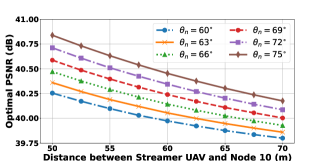
Figure 12: $\mathcal{P}_{n}^{\star}$ vs. $\theta_{n}$ for Streamer UAV

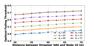
Figure 13: $\beta_{n}^{\star}$ vs. $\theta_{n}$ for Streamer UAV

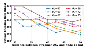
Figure 14: $E_{n}^{\star}$ vs. $\theta_{n}$ for Streamer UAV

Table IV compares PSNR $\mathcal{P}_{i}$, fading threshold $\beta_{i}$, and encoding rate $E_{i}$ for individual ($E_{i}^{\star}$ or $\beta_{i}^{\star}$) or joint ($\beta_{i}^{\star},E_{i}^{\star}$) optimized parameters. In individual optimization, the fading threshold $\beta_{i}$ and encoding rate $E_{i}$ are set to 5 and 2 for LoS and NLoS channels and 304 Kbps for streamer nodes, respectively. As mentioned, our objective is to maximize the average $\mathcal{P}^{\star}$ in the joint optimization (JDVT-EC algorithm), not PSNR $\mathcal{P}_{i}$ for the individual nodes. Accordingly, the JDVT-EC algorithm outperforms the individual optimization in terms of average $\mathcal{P}^{\star}$. However, in terms of individual performance, streamer UAV experiences a higher optimal PSNR $\mathcal{P}^{\star}_{i}$ in the individual optimized $\beta_{i}$ compared to the JDVT-EC algorithm. Moreover, the values of PSNR $\mathcal{P}_{i}$ by different encoding rates $E_{i}$ with optimal fading threshold $\beta_{i}^{\star}$ are demonstrated for streamer nodes in Table V. We define different encoding rates according to the tolerance of the transmission queue as follows: (1) Low Encoding Rate: Nodes set the encoding rates $E_{i}$ randomly between 152 Kbps to 212.8 Kbps. (2) Medium Encoding Rate: Nodes set the encoding rates $E_{i}$ randomly between 273.6 Kbps to 334.4 Kbps. (3) High Encoding Rate: Nodes set the encoding rates $E_{i}$ randomly between 395.2 Kbps to 456 Kbps. From the results in Table V, we note that the optimal PSNR $\mathcal{P}_{i}^{\star}$ achieved by the JDVT-EC algorithm (which uses the optimal encoding rate $E_{i}^{\star}$) outperforms the baselines with low, medium, and high encoding rates $E_{i}$.

VI-B2 JDVT-EC Algorithm Behavior

In Table VI, the optimal fading threshold $\beta_{i}^{\star}$ for 2 LoS (nodes 1 and 2: streamer and interferer UAVs) and 3 NLoS channels (nodes 3, 4, and 5: ground streamers) is represented by different sensitivity parameters $s_{n}$. The sensitivity parameter $s_{n}$ controls the sensitivity of the overall distortion $\mathrm{D}_{n}$ to the packet loss distortion $\mathrm{D}_{n}^{lss}$, which balances the weight between the packet loss distortion $\mathrm{D}_{n}^{lss}$ and the lossy video compression distortion $\mathrm{D}_{n}^{cmp}$. As shown, increasing the sensitivity parameter $s_{n}$ increases the optimal fading threshold $\beta_{i}^{\star}$ since the impact of packet loss distortion $\mathrm{D}_{n}^{lss}$ on the overall distortion $\mathrm{D}_{n}$ increases. Therefore, streamer nodes try to act more conservatively in terms of packet loss. Moreover, the optimal encoding rate $E_{i}^{\star}$ is reported as a function of different sensitivity parameters $s_{n}$. We note that increasing the sensitivity parameter $s_{n}$ decreases the optimal encoding rate $E_{i}^{\star}$ since the JDVT-EC algorithm tries to offset the impact of increasing packet loss distortion $\mathrm{D}_{n}^{lss}$ by decreasing the optimal encoding rate $E_{i}^{\star}$ to have a lower probability of overall loss $\mathbb{P}_{n}^{lss}$. Similarly, Table VI shows the optimal fading threshold $\beta_{i}^{\star}$ by different SINR thresholds $\gamma_{th}$ for streamer nodes. By increasing the SINR threshold $\gamma_{th}$, streamer nodes behave more conservatively and increase the optimal fading threshold $\beta_{i}^{\star}$ to reduce the impact of transmission errors. Therefore, they attempt to decrease the drop in the optimal PSNR $\mathcal{P}_{i}^{\star}$. In addition, the optimal encoding rate $E_{i}^{\star}$ for different SINR thresholds $\gamma_{th}$ is reported. From the results, we note that as the SINR threshold $\gamma_{th}$ increases, streamer nodes decrease their optimal encoding rate $E_{i}^{\star}$ to decrease packet loss. They try to decrease the drop in the optimal PSNR $\mathcal{P}_{i}^{\star}$ by reducing network load. However, modifying the SINR threshold $\gamma_{th}$ has minimum impact on the optimal encoding rate and fading threshold of node 4.

Fig. 11 shows the optimal PSNR $\mathcal{P}_{i}^{\star}$ from the JDVT-EC algorithm for streamer nodes (nodes 1 to 5) by different sensitivity parameters $s_{n}$. Clearly, as the sensitivity parameter $s_{n}$ increases for streamer nodes, the optimal PSNR $\mathcal{P}_{i}^{\star}$ decreases since the impact of the packet loss distortion $\mathrm{D}_{n}^{lss}$ increases on the overall distortion $\mathrm{D}_{n}$. Also, the degradation of the optimal PSNR $\mathcal{P}_{i}^{\star}$ for streamer nodes with lower optimal PSNR $\mathcal{P}_{i}^{\star}$ (nodes 1 and 4) is higher than other streamers (nodes 2, 3, and 5). Similarly, the optimal PSNR $\mathcal{P}_{i}^{\star}$ by optimizing fading threshold $\beta_{i}$ and encoding rate $E_{i}$ is represented for different SINR thresholds $\gamma_{th}$ in Fig. 11. Indeed, as the SINR threshold $\gamma_{th}$ increases, the streamer nodes suffer a higher transmission error, and thus the packet loss distortion $\mathrm{D}_{n}^{lss}$ increases. As a result, the optimal PSNR $\mathcal{P}_{i}^{\star}$ from the JDVT-EC algorithm degrades by increasing the SINR threshold $\gamma_{th}$. Moreover, the impact of changing SINR threshold $\gamma_{th}$ is negligible on node 4 as an NLoS ground streamer with low optimal PSNR $\mathcal{P}_{i}^{\star}$, which streams in a crowded area.

VI-C Spatial Performance

In Fig. 11, the optimal PSNR $\mathcal{P}_{n}^{\star}$ heatmap for 25 different locations in 100$\times$100 $\text{m}^{2}$ area is represented for streamer UAV at 50 m altitude while the optimal fading threshold $\beta_{n}^{\star}$ and optimal encoding rate $E_{n}^{\star}$ are shown inside of each squared location. As the streamer UAV gets closer to its associated ground node 10 (-10.22 m, -29.74 m), it can efficiently serve node 10 in the presence of interferer nodes and experiences a higher optimal PSNR $\mathcal{P}_{n}^{\star}$. Moreover, the streamer UAV increases its optimal encoding rate $E_{n}^{\star}$ due to good channel condition and optimal fading threshold $\beta_{n}^{\star}$ since the range of fading threshold extends near node 10.

In Fig. 14, the optimal PSNR $\mathcal{P}^{\star}_{n}$ by the JDVT-EC algorithm is indicated for different distances d = {50, 52.5, 55, 57.5, 60, 62.5, 65, 67.5, 70} and elevation angles $\Theta$ = {60, 63, 66, 69, 72, 75} between the streamer UAV and node 10. Increasing the distance between the streamer UAV and its ground node (i.e., node 10) gradually degrades the optimal PSNR $\mathcal{P}^{\star}_{n}$. By increasing the elevation angle $\theta_{n}$, the streamer UAV establishes a better LoS channel with node 10 since the LoS probability $\mathbb{P}_{L}(d_{i})$ increases; thus, the optimal PSNR $\mathcal{P}^{\star}_{n}$ increases. Overall, the average PSNR $\bar{\mathcal{P}}_{n}$ for all distances d and elevation angles $\Theta$ when the streamer UAV serving in this specific spatial area would be $\bar{\mathcal{P}}_{n}=40.22$ dB. Figs. 14 and 14 illustrate the optimal fading threshold $\beta_{n}^{\star}$ and optimal encoding rate $E_{n}^{\star}$ for the streamer UAV by changing the distance $d_{n}$ and elevation angle $\theta_{n}$ between the streamer UAV and node 10. As the distance increases, the optimal fading threshold $\beta_{n}^{\star}$ increases. Conversely, the optimal encoding rate $E_{n}^{\star}$ generally drops due to degraded channel conditions.

VII Conclusion

In this paper, we investigated the problem of distributed transmission control and video streaming optimization for UAVs operating in unlicensed spectrum bands. We developed an analytical framework that jointly considers cross-layer parameters, including the channel parameters at the PHY layer, queuing parameters at the MAC layer, and video encoding rate at the application layer. Using this framework, we studied the throughput and PSNR according to the overall packet loss $\mathbb{P}_{n}^{lss}(\boldsymbol{\beta})$ and lossy video compression distortion $\mathrm{D}_{n}^{cmp}(\mathrm{E}_{n})$. In our proposed solution, we introduced two algorithms, namely the DTC algorithm for distributed transmission control and the JDVT-EC algorithm for joint distributed video transmission and encoder control to optimize the video encoding rate $\mathrm{E}_{n}$ and the fading threshold $\beta_{n}$ for each source node. The objective function is to maximize the average throughput and PSNR over all nodes. Through extensive numerical evaluations, we demonstrated the efficacy of our algorithms and verified that they consistently achieved optimal solutions.

Appendix A Proof of Buffer Overflow Model

As mentioned, the probability of exceeding the buffer capacity in a certain state $i$ can be defined as:

$$\begin{aligned} \overline{\mathbb{P}_{i,i+1}}&=\mathbb{P}[x_{1}+...+x_{i+1}>b_{n}|x_{1}+...+x_{i}\leq b_{n}]\\ &=\frac{\int_{0}^{b_{n}}\mathbb{P}[x_{i+1}>b_{n}-x]f_{x_{1}+...+x_{i}}(x)dx}{\mathbb{P}[x_{1}+...+x_{i}\leq b_{n}]},\end{aligned}$$ (16)

where $f_{x_{1}+...+x_{i}}(x)$ represents the PDF of an i-Erlang distribution. Consequently, the complement of $\overline{\mathbb{P}_{i,i+1}}$ without occurring buffer overflow, can be expressed as:

$$\mathbb{P}_{i,i+1}=1-\overline{\mathbb{P}_{i,i+1}}=\frac{1-\sum_{j=0}^{i}\frac{\tilde{b}_{n}^{j}}{j!}e^{-\tilde{b}_{n}}}{1-\sum_{j=0}^{i-1}\frac{\tilde{b}_{n}^{j}}{j!}e^{-\tilde{b}_{n}}}.$$ (17)

Based on the Markov chain, the local balance equation is given by $\pi_{i+1}=\rho_{n}(\beta_{n})\mathbb{P}_{i,i+1}\pi_{i}$, where $\rho_{n}(\beta_{n})=\frac{\lambda_{n}T^{slt}_{n}}{\mu_{n}(\beta_{n})}$ denotes the offered load. Then, $\pi_{i}$ can be derived as:

$$\pi_{i}=\rho_{n}^{i}(\beta_{n})\Big{(}\prod_{j=0}^{i-1}\mathbb{P}_{j,j+1}\Big{)}\pi_{0}=\rho_{n}^{i}(\beta_{n})\Big{(}1-\sum_{j=0}^{i-1}\frac{\tilde{b}_{n}^{j}}{j!}e^{-\tilde{b}_{n}}\Big{)}\pi_{0}.$$

Now, utilizing $\sum_{j=0}^{\infty}\pi_{j}=1$ and taking into account that $\rho_{n}(\beta_{n})<1$, $\pi_{0}$ can be calculated as:

$$\pi_{0}=\frac{1-\rho_{n}(\beta_{n})}{1-\rho_{n}(\beta_{n})e^{-\tilde{b}_{n}(1-\rho_{n}(\beta_{n}))}}.$$ (18)

Finally, the probability of buffer overflow is approximated as:

$$\mathbb{P}_{n}^{ov}(\beta_{n})\approx\sum_{i=0}^{\infty}\overline{\mathbb{P}_{i,i+1}}\pi_{i}=\frac{(1-\rho_{n}(\beta_{n}))e^{-\tilde{b}_{n}(1-\rho_{n}(\beta_{n}))}}{1-\rho_{n}(\beta_{n})e^{-\tilde{b}_{n}(1-\rho_{n}(\beta_{n}))}}.$$

Appendix B Parameters of Log-normal Distribution

As mentioned, $\mu(\boldsymbol{\beta}_{-n})$ and $\sigma(\boldsymbol{\beta}_{-n})$ are the location and scale parameters in Log-normal distribution, which are given by:

$$\mu(\boldsymbol{\beta}_{-n})=\ln(\tilde{\mathbb{E}}[I_{n}^{f}(\boldsymbol{\beta}_{-n})])-\frac{1}{2}\ln\Big{(}1+\frac{\tilde{\mathbb{D}}[I_{n}^{f}(\boldsymbol{\beta}_{-n})]}{(\tilde{\mathbb{E}}[I_{n}^{f}(\boldsymbol{\beta}_{-n})])^{2}}\Big{)},$$

$$\sigma(\boldsymbol{\beta}_{-n})=\sqrt{\ln\Big{(}1+\frac{\tilde{\mathbb{D}}[I_{n}^{f}(\boldsymbol{\beta}_{-n})]}{(\tilde{\mathbb{E}}[I_{n}^{f}(\boldsymbol{\beta}_{-n})])^{2}}\Big{)}},$$

where $\tilde{\mathbb{E}}[I_{n}^{f}(\boldsymbol{\beta}_{-n})]$ and $\tilde{\mathbb{D}}[I_{n}^{f}(\boldsymbol{\beta}_{-n})]$ are the first and second order moments of $I_{n}^{f}(\boldsymbol{\beta}_{-n})$, which are shown as:

$$\tilde{\mathbb{E}}[I_{n}^{f}(\boldsymbol{\beta}_{-n})]=\sum_{m\in\boldsymbol{N}\backslash n}\mathbb{E}\bigl{[}P_{m}(\hat{h}_{m}^{f})^{2}(\tilde{h}_{m}^{f})^{2}\alpha_{m}^{f}(\beta_{m})\bigl{]}$$

$$=\sum_{m\in\boldsymbol{N}\backslash n}\frac{P_{m}(\hat{h}_{m}^{f})^{2}\mu_{m}(\beta_{m})}{|\boldsymbol{F}|}\int_{\beta_{m}}^{\infty}x^{2}\mathbb{P}(\tilde{h}_{m}^{f}=x)dx,$$

$$\tilde{\mathbb{D}}[I_{n}^{f}(\boldsymbol{\beta}_{-n})]=\sum_{m\in\boldsymbol{N}\backslash n}\Big{(}\frac{P_{m}(\hat{h}_{m}^{f})^{2}\mu_{m}(\beta_{m})}{|\boldsymbol{F}|}\Big{)}^{2}\times$$

$$\int_{\beta_{m}}^{\infty}x^{4}\mathbb{P}(\tilde{h}_{m}^{f}=x)dx+\sum_{m_{1}\neq m_{2}}\frac{P_{m_{1}}(\hat{h}_{m_{1}}^{f})^{2}\mu_{m_{1}}(\beta_{m_{1}})}{|\boldsymbol{F}|}\times$$

$$\int_{\beta_{m_{1}}}^{\infty}x^{2}\mathbb{P}(\tilde{h}_{m_{1}}^{f}=x)dx\frac{P_{m_{2}}(\hat{h}_{m_{2}}^{f})^{2}\mu_{m_{2}}(\beta_{m_{2}})}{|\boldsymbol{F}|}\times$$

$$\int_{\beta_{m_{2}}}^{\infty}x^{2}\mathbb{P}(\tilde{h}_{m_{2}}^{f}=x)dx-(\tilde{\mathbb{E}}[I_{n}^{f}(\boldsymbol{\beta}_{-n})])^{2}.$$

Here, $\mu_{m}(\beta_{m})$ and $\mathbb{P}(\tilde{h}_{m}^{f}=x)$ depend on the type of channel between the interferer node $m$ and the destination.

Appendix C Concavity of $\mathbb{R}_{n}$ and $\mathcal{P}_{n}$ with Respect to $\beta_{n}$

Only need to prove the convexity of $\mathbb{P}_{n}^{lss}$ with respect to $\beta_{n}$ i.e. $\frac{\partial^{2}\mathbb{P}_{n}^{lss}}{\partial\beta_{n}^{2}}>0$. Thus, we have:

$$\frac{\partial\mathbb{P}^{lss}_{n}}{\partial\beta_{n}}=\frac{\partial\mathbb{P}^{err}_{n}}{\partial\beta_{n}}+\frac{\partial\mathbb{P}^{dly}_{n}}{\partial\beta_{n}},$$ (19)

in which $\mathbb{P}_{n}^{ov}(\beta_{n})$ is ignored due to its negligible value and for the sake of simplicity. Hence, $\frac{\partial\mathbb{P}_{n}^{lss}}{\partial\beta_{n}}$ can be expressed as:

$$\frac{\partial\mathbb{P}_{n}^{lss}}{\partial\beta_{n}} =-\mathbb{P}(\tilde{h}_{n}^{f}=\beta_{n})v_{n}(X,\boldsymbol{\beta}_{-n})$$

$$+\frac{|\boldsymbol{F}|T_{n}^{th}}{T^{slt}_{n}}\mathbb{P}_{n}^{dly}(\beta_{n})\mathbb{P}(\tilde{h}_{n}^{f}<\beta_{n})^{|\boldsymbol{F}|-1}\mathbb{P}(\tilde{h}_{n}^{f}=\beta_{n}),$$

where $X=\frac{P_{n}\hat{h}_{n}^{2}}{\gamma_{th}}\beta_{n}^{2}-\sigma^{2}$. Then,

$$\frac{\partial^{2}\mathbb{P}^{lss}_{n}}{\partial\beta_{n}^{2}}=\frac{\partial^{2}\mathbb{P}^{err}_{n}}{\partial\beta_{n}^{2}}+\frac{\partial^{2}\mathbb{P}^{dly}_{n}}{\partial\beta_{n}^{2}}.$$ (20)

Here, $\frac{\partial^{2}\mathbb{P}_{n}^{err}}{\partial\beta_{n}^{2}}$ and $\frac{\partial^{2}\mathbb{P}_{n}^{dly}}{\partial\beta_{n}^{2}}$ can be calculated as:

$$\frac{\partial^{2}\mathbb{P}_{n}^{err}}{\partial\beta_{n}^{2}} =e^{-\frac{\beta_{n}^{2}+b^{2}}{2}}\Big{(}(\beta_{n}^{2}-1)I_{0}(\beta_{n}b)-\beta_{n}bI_{1}(\beta_{n}b)\Big{)}$$

$$\times v_{n}(X,\boldsymbol{\beta}_{-n})-\mathbb{P}(\tilde{h}_{n}^{f}=\beta_{n})\frac{\partial v_{n}(X,\boldsymbol{\beta}_{-n})}{\partial\beta_{n}},$$

where $\frac{\partial v_{n}(X,\boldsymbol{\beta}_{-n})}{\partial\beta_{n}}<0$ and $0\leq v_{n}(X,\boldsymbol{\beta}_{-n})\leq 1$. Using the upper bound of fading threshold and $I_{0}(\beta_{n}b)>I_{1}(\beta_{n}b)$, $(\beta_{n}^{2}-1)I_{0}(\beta_{n}b)>\beta_{n}bI_{1}(\beta_{n}b)$, we have $\frac{\partial^{2}\mathbb{P}_{n}^{err}}{\partial\beta_{n}^{2}}>0$. Then,

$$\frac{\partial^{2}\mathbb{P}_{n}^{dly}}{\partial\beta_{n}^{2}}=\frac{\partial\mathbb{P}_{n}^{dly}}{\partial\beta_{n}}\frac{|\boldsymbol{F}|T_{n}^{th}}{T^{slt}_{n}}\mathbb{P}(\tilde{h}_{n}^{f}<\beta_{n})^{|\boldsymbol{F}|-1}\mathbb{P}(\tilde{h}_{n}^{f}=\beta_{n})+$$

$$\mathbb{P}_{n}^{dly}(\beta_{n})\frac{|\boldsymbol{F}|T_{n}^{th}}{T^{slt}_{n}}(|\boldsymbol{F}|-1)\mathbb{P}(\tilde{h}_{n}^{f}<\beta_{n})^{|\boldsymbol{F}|-2}\mathbb{P}(\tilde{h}_{n}^{f}=\beta_{n})^{2}$$

$$+\frac{\partial\mathbb{P}(\tilde{h}_{n}^{f}=\beta_{n})}{\partial\beta_{n}}\frac{|\boldsymbol{F}|T_{n}^{th}}{T^{slt}_{n}}\mathbb{P}_{n}^{dly}(\beta_{n})\mathbb{P}(\tilde{h}_{n}^{f}<\beta_{n})^{|\boldsymbol{F}|-1},$$

where $\frac{\partial\mathbb{P}_{n}^{dly}}{\partial\beta_{n}}>0$. Assuming $\frac{|\boldsymbol{F}|T_{n}^{th}}{T^{slt}_{n}}\gg 1$ to prove $\frac{\partial^{2}\mathbb{P}_{n}^{dly}}{\partial\beta_{n}^{2}}>0$, need to demonstrate:

$$\frac{\partial\mathbb{P}_{n}^{dly}}{\partial\beta_{n}}\Big{(}1+\frac{1-\beta_{n}^{2}}{\beta_{n}}+\frac{bI_{1}(\beta_{n}b)}{I_{0}(\beta_{n}b)}\Big{)}+|\boldsymbol{F}|-1>0.$$

This inequality can be numerically verified as long as the upper bound of fading threshold holds.

Appendix D Concavity of $\mathcal{P}_{n}$ with Respect to $\mathrm{E}_{n}$

To prove the concavity of $\mathcal{P}_{n}$ related to $E_{n}$, it is sufficient to prove the convexity of $\ln\mathrm{D}_{n}$ with respect to $E_{n}$ as follows:

$$\frac{\partial^{2}\mathrm{D}_{n}}{\partial\mathrm{E}_{n}^{2}}\mathrm{D}_{n}-2\Big{(}\frac{\partial\mathrm{D}_{n}}{\partial\mathrm{E}_{n}}\Big{)}^{2}\geq 0,$$ (21)

where the first and second derivatives of $\mathrm{D}_{n}$ are provided as:

$$\frac{\partial\mathrm{D}_{n}}{\partial\mathrm{E}_{n}}=-\frac{\theta_{0}}{(\mathrm{E}_{n}-E_{0})^{2}}+\frac{s_{n}T_{n}^{th}}{L_{n}}\mathbb{P}_{n}^{dly}(\beta_{n}),$$

$$\frac{\partial^{2}\mathrm{D}_{n}}{\partial\mathrm{E}_{n}^{2}}=\frac{2\theta_{0}}{(\mathrm{E}_{n}-E_{0})^{3}}+s_{n}(\frac{T_{n}^{th}}{L_{n}})^{2}\mathbb{P}_{n}^{dly}(\beta_{n}).$$

Here, it can be obtained:

$$\frac{\partial^{2}\mathrm{D}_{n}}{\partial\mathrm{E}_{n}^{2}}\mathrm{D}_{n}=\frac{2\theta_{0}D_{0}}{(\mathrm{E}_{n}-E_{0})^{3}}+s_{n}D_{0}(\frac{T_{n}^{th}}{L_{n}})^{2}\mathbb{P}_{n}^{dly}(\beta_{n})+$$

$$\frac{2\theta_{0}^{2}}{(\mathrm{E}_{n}-E_{0})^{4}}+\frac{s_{n}\theta_{0}}{\mathrm{E}_{n}-E_{0}}(\frac{T_{n}^{th}}{L_{n}})^{2}\mathbb{P}_{n}^{dly}(\beta_{n})+$$

$$\frac{2s_{n}\theta_{0}\mathbb{P}_{n}^{lss}(\boldsymbol{\beta})}{(\mathrm{E}_{n}-E_{0})^{3}}+(\frac{s_{n}T_{n}^{th}}{L_{n}})^{2}\mathbb{P}_{n}^{dly}(\beta_{n})\mathbb{P}_{n}^{lss}(\boldsymbol{\beta}),$$

$$2\Big{(}\frac{\partial\mathrm{D}_{n}}{\partial\mathrm{E}_{n}}\Big{)}^{2}=\frac{2\theta_{0}^{2}}{(\mathrm{E}_{n}-E_{0})^{4}}+2(\frac{s_{n}T_{n}^{th}}{L_{n}})^{2}\mathbb{P}_{n}^{dly}(\beta_{n})^{2}$$

$$-\frac{4s_{n}\theta_{0}T_{n}^{th}\mathbb{P}_{n}^{dly}(\beta_{n})}{(\mathrm{E}_{n}-E_{0})^{2}L_{n}},$$

since $\mathbb{P}_{n}^{lss}(\boldsymbol{\beta})>\mathbb{P}_{n}^{dly}(\beta_{n})$, we can get the following inequality:

$$\frac{2\theta_{0}D_{0}}{(\mathrm{E}_{n}-E_{0})^{3}}+s_{n}D_{0}(\frac{T_{n}^{th}}{L_{n}})^{2}\mathbb{P}_{n}^{dly}(\beta_{n})+$$

$$\frac{s_{n}\theta_{0}}{\mathrm{E}_{n}-E_{0}}(\frac{T_{n}^{th}}{L_{n}})^{2}\mathbb{P}_{n}^{dly}(\beta_{n})+\frac{2s_{n}\theta_{0}\mathbb{P}_{n}^{lss}(\boldsymbol{\beta})}{(\mathrm{E}_{n}-E_{0})^{3}}$$

$$+\frac{4s_{n}\theta_{0}T_{n}^{th}\mathbb{P}_{n}^{dly}(\beta_{n})}{(\mathrm{E}_{n}-E_{0})^{2}L_{n}}-(\frac{s_{n}T_{n}^{th}}{L_{n}})^{2}\mathbb{P}_{n}^{dly}(\beta_{n})^{2}\geq 0,$$

where $\theta_{0}\gg s_{n}$, $\mathbb{P}_{n}^{dly}(\beta_{n})>\mathbb{P}_{n}^{dly}(\beta_{n})^{2}$, and $\frac{T_{n}^{th}}{L_{n}}\ll 1$. Thus, this inequality can be proved.

Algorithm 5 Local Coordinate Search (LCS)

1:function LCS($\mathrm{E}_{n}$, $\boldsymbol{\beta}$, $\boldsymbol{stp}$, $bst$, $\boldsymbol{\beta}^{max}$, $swt$)

2:    if $swt=0$ then $\boldsymbol{stp}_{x}\leftarrow\boldsymbol{stp}_{\beta}$, $x\leftarrow\beta_{n}$

3:    else if $swt=1$ then $\boldsymbol{stp}_{x}\leftarrow\boldsymbol{stp}_{\lambda}$, $x\leftarrow\frac{\mathrm{E}_{n}}{L_{n}}$

4:    end if

5:    $flg\leftarrow 0$, $k\leftarrow 0$, $stp_{x}\leftarrow stp^{acc}_{x}*stp^{div}_{x}$

6:    while $flg\neq 4$ do

7:       while $flg=0$ do $stp_{x}\leftarrow\frac{stp_{x}}{stp^{div}_{x}}$

8:          if $swt=0$ and $x+stp_{x}<\beta^{max}_{n}$ then

9:             $x\leftarrow x+stp_{x}$

10:          else if $swt=1$ then $x\leftarrow x+stp_{x}$

11:          end if

12:          $can\leftarrow\mathcal{P}_{n}(\mathrm{E}_{n},\boldsymbol{\beta})$ or $\mathbb{R}_{n}(\boldsymbol{\beta})$

13:          if $can>bst$ then $bst\leftarrow can$, $k\leftarrow k+1$

14:          else if $k\neq 0$ and $stp_{x}^{div}\neq 1$ then

15:             $flg\leftarrow 1$, $x\leftarrow x-stp_{x}$

16:          else if $k\neq 0$ and $stp_{x}^{div}=1$ then

17:             $flg\leftarrow 4$, $x\leftarrow x-stp_{x}$

18:          else if $k=0$ then $flg\leftarrow 2$, $x\leftarrow x-stp_{x}$

19:             $stp_{x}\leftarrow stp_{x}*stp^{div}_{x}$

20:          end if

21:       end while

22:       while $flg=1$ do $stp_{x}\leftarrow stp_{x}*stp^{div}_{x}$

23:          if $stp_{x}<stp^{acc}_{x}$ then $flg\leftarrow 4$

24:             break

25:          end if

26:          if $swt=0$ and $x+stp_{x}<\beta^{max}_{n}$ then

27:             $x\leftarrow x+stp_{x}$

28:          else if $swt=1$ then $x\leftarrow x+stp_{x}$

29:          end if

30:          $can\leftarrow\mathcal{P}_{n}(\mathrm{E}_{n},\boldsymbol{\beta})$ or $\mathbb{R}_{n}(\boldsymbol{\beta})$

31:          if $can>bst$ then $bst\leftarrow can$

32:          else: $x\leftarrow x-stp_{x}$

33:             if $stp_{x}=stp^{acc}_{x}$ then

34:                $flg\leftarrow 2$, $stp_{x}\leftarrow stp_{x}*stp^{div}_{x}$

35:             end if

36:          end if

37:       end while

38:       while $flg=2$ do $stp_{x}\leftarrow\frac{stp_{x}}{stp^{div}_{x}}$

39:          if $x-stp_{x}>0$ then $x\leftarrow x-stp_{x}$

40:          end if

41:          $can\leftarrow\mathcal{P}_{n}(\mathrm{E}_{n},\boldsymbol{\beta})$ or $\mathbb{R}_{n}(\boldsymbol{\beta})$

42:          if $can>bst$ then $bst\leftarrow can$

43:          else if $stp_{x}^{div}\neq 1$ then: $flg\leftarrow 3$, $x\leftarrow x+stp_{x}$

44:          else if $stp_{x}^{div}=1$ then: $flg\leftarrow 4$, $x\leftarrow x+stp_{x}$

45:          end if

46:       end while

47:       while $flg=3$ do $stp_{x}\leftarrow stp_{x}*stp^{div}_{x}$

48:          if $stp_{x}<stp^{acc}_{x}$ then $flg\leftarrow 4$

49:             break

50:          end if

51:          if $x-stp_{x}>0$ then $x\leftarrow x-stp_{x}$

52:          end if

53:          $can\leftarrow\mathcal{P}_{n}(\mathrm{E}_{n},\boldsymbol{\beta})$ or $\mathbb{R}_{n}(\boldsymbol{\beta})$

54:          if $can>bst$ then $bst\leftarrow can$

55:          else: $x\leftarrow x+stp_{x}$

56:             if $stp_{x}=stp^{acc}_{x}$ then

57:                $flg\leftarrow 0$, $stp_{x}\leftarrow stp_{x}*stp^{div}_{x}$

58:             end if

59:          end if

60:       end while

61:    end while

62:    if $swt=1$ then $x\leftarrow x*L_{n}$

63:    end if

64:    return $x$

65:end function

Appendix E Local Coordiante Search (LCS) Algorithm

The Local Coordinate Search (LCS) Algorithm aims to determine the optimal value of $x=\{\lambda_{n},\beta_{n}\}$ for each node in each iteration. In this algorithm, the decision variable is selected by a switch ($swt$), and flags handle the coordinate search direction, step size, and where to terminate the algorithm. Furthermore, $\boldsymbol{stp}=\{\boldsymbol{stp}_{\beta},\boldsymbol{stp}_{\lambda}\}=\{\{stp^{div}_{\beta},stp^{acc}_{\beta}\},\{stp^{div}_{\lambda},stp^{acc}_{\lambda}\}\}$ includes the step divider $stp^{div}_{x}$, which changes the step size proportionally, and step accuracy $stp^{acc}_{x}$, which controls the accuracy of the decision variable and stops the algorithm according to the step size.

References

- Zhan and Huang [2020] C. Zhan and R. Huang, “Energy eff. adaptive video streaming with rotary-wing UAV,” IEEE Trans. on Vehicular Tech., 2020.
- Khan et al. [2024] N. Khan, A. Ahmad, A. Wakeel, Z. Kaleem, B. Rashid, and W. Khalid, “Efficient UAVs deployment and resource allocation in UAV-relay assisted public safety networks for video transmission,” IEEE Access, 2024.
- Yuan et al. [2017] Z. Yuan, J. Jin, J. Chen, L. Sun, and G.-M. Muntean, “Comprose: Shaping future public safety communities with prose-based UAVs,” IEEE Communications Magazine, 2017.
- Chintareddy et al. [2023] S. R. Chintareddy, K. Roach, K. Cheung, and M. Hashemi, “Collaborative wideband spectrum sensing and scheduling for networked UAVs in UTM systems,” GLOBECOM 2023 - 2023 IEEE Global Communications Conference, 2023.
- Sharma et al. [2023] M. K. Sharma, C.-F. Liu, I. Farhat, N. Sehad, W. Hamidouche, and M. Debbah, “UAV immersive video streaming: A comprehensive survey, benchmarking, and open challenges,” arXiv:2311.00082, 2023.
- Badnava et al. [2022] B. Badnava, S. Reddy Chintareddy, and M. Hashemi, “QoE-centric multi-user mmwave scheduling: A beam alignment and buffer predictive approach,” 2022 IEEE International Symposium on Information Theory (ISIT), 2022.
- Meng et al. [2022] K. Meng, Q. Wu, S. Ma, W. Chen, and T. Q. S. Quek, “UAV trajectory and beamforming optimization for integrated periodic sensing and comm.” IEEE Wireless Comm. Letters, 2022.
- Badnava et al. [2023] B. Badnava, K. Roach, K. Cheung, M. Hashemi, and N. B. Shroff, “Energy-eff. deadline-aware edge computing: Bandit learning with partial observations in multi-channel systems,” GLOBECOM 2023 - 2023 IEEE Global Comm. Conf., 2023.
- Reddy Chintareddy et al. [2023] S. Reddy Chintareddy, K. Roach, K. Cheung, and M. Hashemi, “Collaborative wideband spectrum sensing and scheduling for networked UAVs in UTM systems,” arXiv:2308.05036, 2023.
- Bithas and Moustakas [2023] P. S. Bithas and A. L. Moustakas, “Generalized UAV selection with distributed trans. policies,” IEEE Trans. on Comm., 2023.
- Guan et al. [2016] Z. Guan, T. Melodia, and G. Scutari, “To transmit or not to transmit? distributed queueing games in infrastructureless wireless networks,” IEEE/ACM Trans. on Networking, 2016.
- Bithas et al. [2020] P. S. Bithas, V. Nikolaidis, A. G. Kanatas, and G. K. Karagiannidis, “UAV-to-ground communications: Channel modeling and UAV selection,” IEEE Trans. on Communications, 2020.
- Cui et al. [2019] J. Cui, Z. Ding, Y. Deng, and A. Nallanathan, “Model-free based automated trajectory optimization for UAVs toward data trans.” 2019 IEEE Global Comm. Conf. (GLOBECOM), 2019.
- Wang et al. [2021] K. Wang, C. Pan, H. Ren, W. Xu, L. Zhang, and A. Nallanathan, “Packet error prob. and effective throughput for ultra-reliable and low-latency UAV comm.” IEEE Trans. on Comm., 2021.
- Solanki et al. [2023] S. Solanki, V. Singh, S. Gautam, J. Querol, and S. Chatzinotas, “Short-packet communication assisted reliable control of UAV for optimum coverage range,” ICC 2023 - IEEE International Conference on Communications, 2023.
- Pan et al. [2020] G. Pan, H. Lei, J. An, S. Zhang, and M.-S. Alouini, “On the secrecy of UAV systems with linear trajectory,” IEEE Transactions on Wireless Communications, 2020.
- Hellaoui et al. [2019] H. Hellaoui, A. Chelli, M. Bagaa, T. Taleb, and M. Pätzold, “Towards eff. control of mobile network-enabled UAVs,” 2019 IEEE Wireless Comm. and Networking Conf. (WCNC), 2019.
- Tian et al. [2016] J. Tian, H. Zhang, D. Wu, and D. Yuan, “Interference-aware cross-layer design for dist. video trans. in wireless networks,” IEEE Trans. on Circuits and Systems for Video Tech., 2016.
- Li et al. [2022] T. Li, C. Li, C. Yang, J. Shao, Y. Zhang, L. Pang, L. Chang, L. Yang, and Z. Han, “A mean field game-theoretic cross-layer optimization for multi-hop swarm UAV communications,” Journal of Communications and Networks, 2022.
- Zhan et al. [2021] C. Zhan, H. Hu, X. Sui, Z. Liu, J. Wang, and H. Wang, “Joint resource allocation and 3D aerial trajectory design for video streaming in UAV communication systems,” IEEE Transactions on Circuits and Systems for Video Technology, 2021.
- Chen et al. [2020] Y. Chen, H. Zhang, and Y. Hu, “Optimal power and bandwidth allocation for multiuser video streaming in UAV relay networks,” IEEE Transactions on Vehicular Technology, 2020.
- Zhang and Chakareski [2022] L. Zhang and J. Chakareski, “UAV-assisted edge computing and streaming for wireless virtual reality: Analysis, algo. design, and performance guarantees,” IEEE Trans. on Vehicular Tech., 2022.
- Xie et al. [2022] J. Xie, Z. Wang, and Y. Chen, “Joint caching and user association optimization for adaptive bitrate video streaming in UAV-assisted cellular networks,” IEEE Access, 2022.
- Liao et al. [2022] J. Liao, C. Zhan, Y. Yang, and B. Zeng, “QoE maximization for multi-antenna UAV-enabled video streaming,” GLOBECOM 2022 - 2022 IEEE Global Communications Conference, 2022.
- Ghazikor et al. [2024] M. Ghazikor, K. Roach, K. Cheung, and M. Hashemi, “Interference-aware queuing analysis for distributed transmission control in UAV networks,” arXiv:2401.11084, 2024.
- Ghazikor et al. [2023] ——, “Exploring the interplay of interference and queues in unlicensed spectrum bands for UAV networks,” 2023 57th Asilomar Conference on Signals, Systems, and Computers, 2023.
- Kim and Lee [2018] M. Kim and J. Lee, “Outage probability of UAV communications in the presence of interference,” 2018 IEEE Global Communications Conference (GLOBECOM), 2018.
- Mohammed et al. [2021] I. Mohammed, I. B. Collings, and S. V. Hanly, “Line of sight probability prediction for UAV comm.” 2021 IEEE International Conf. on Comm. Workshops (ICC Workshops), 2021.
- Kim and Lee [2019] M. Kim and J. Lee, “Impact of an interfering node on unmanned aerial vehicle comm.” IEEE Trans. on Vehicular Tech., 2019.
- Ren et al. [2011] Z. Ren, G. Wang, Q. Chen, and H. Li, “Modelling and sim. of rayleigh fading, path loss, and shadowing fading for wireless mobile networks,” Sim. Modelling Practice and Theory, 2011.
- Azari et al. [2018] M. M. Azari, F. Rosas, K.-C. Chen, and S. Pollin, “Ultra reliable UAV communication using altitude and cooperation diversity,” IEEE Transactions on Communications, 2018.
- Kumar et al. [2023] P. Kumar, S. Bhattacharyya, S. Darshi, S. Majhi, A. A. Almohammedi, and S. Shailendra, “Outage analysis using probabilistic channel model for drone assisted multi-user coded cooperation system,” IEEE Trans. on Vehicular Tech., 2023.
- Zhou et al. [2018] L. Zhou, Z. Yang, S. Zhou, and W. Zhang, “Coverage probability analysis of UAV cellular networks in urban environments,” 2018 IEEE International Conference on Communications Workshops (ICC Workshops), 2018.
- Zhu et al. [2005] X. Zhu, E. Setton, and B. Girod, “Congestion–distortion optimized video transmission over ad hoc networks,” Signal Processing: Image Communication, 2005.
- Gross et al. [2008] D. Gross, J. F. Shortle, J. M. Thompson, and C. M. Harris, Fundamentals of Queueing Theory. Wiley-Interscience, 2008.
- Berahas et al. [2019] A. S. Berahas, R. Bollapragada, N. S. Keskar, and E. Wei, “Balancing communication and computation in distributed optimization,” IEEE Transactions on Automatic Control, 2019.
- Tang et al. [2021] X.-W. Tang, X.-L. Huang, and F. Hu, “QoE-driven UAV-enabled pseudo-analog wireless video broadcast: A joint optimization of power and trajectory,” IEEE Transactions on Multimedia, 2021.
- Recht and Fridovich-Keil [2019] B. Recht and S. Fridovich-Keil, “Choosing the step size: Intuitive line search algo. with eff. convergence,” OPT2019: 11th Annual Workshop on Optimization for Machine Learning, 2019.