A consistently adaptive trust-region method

Abstract

Adaptive trust-region methods attempt to maintain strong convergence guarantees without depending on conservative estimates of problem properties such as Lipschitz constants. However, on close inspection, one can show existing adaptive trust-region methods have theoretical guarantees with severely suboptimal dependence on problem properties such as the Lipschitz constant of the Hessian. For example, TRACE developed by Curtis et al. obtains a $O(\Delta_{f}L^{3/2}\epsilon^{-3/2})+\tilde{O}(1)$ iteration bound where $L$ is the Lipschitz constant of the Hessian. Compared with the optimal $O(\Delta_{f}L^{1/2}\epsilon^{-3/2})$ bound this is suboptimal with respect to $L$. We present the first adaptive trust-region method which circumvents this issue and requires at most $O(\Delta_{f}L^{1/2}\epsilon^{-3/2})+\tilde{O}(1)$ iterations to find an $\epsilon$-approximate stationary point, matching the optimal iteration bound up to an additive logarithmic term. Our method is a simple variant of a classic trust-region method and in our experiments performs competitively with both ARC and a classical trust-region method.

1 Introduction

Second-order methods are known to quickly and accurately solve sparse nonconvex optimization problems that, for example, arise in optimal control [1], truss design [2], AC optimal power flow [3], and PDE constrained optimization [4]. Recently, there has also been a large push to extend second-order methods to tackle machine learning problems by coupling them with carefully designed subproblem solvers [5, 6, 7, 8, 9, 10, 11, 12, 13, 14, 15, 16, 17, 18, 19].

Much of the early theory for second-order methods focused on showing fast local convergence and (eventual) global convergence [20, 21, 22, 23, 24, 25, 26, 27, 28, 29]. These proofs of global convergence, unsatisfactorily, rested on showing at each iteration second-order methods reduced the function value almost as much as gradient descent [22, Theorem 4.5] [30, Theorem 3.2.], this is despite the fact that in practice second-order methods require far fewer iterations. In 2006, Nesterov and Polyak [31] partially resolved this inconsistency by introducing a new second-order method, cubic regularized Newton’s method (CRN). Their method can be used to find stationary points of multivariate and possibly nonconvex functions $f:{\bf R}^{n}\rightarrow{\bf R}$. Their convergence results assumes the optimality gap

$$\Delta_{f}:=f(x_{1})-\inf_{x\in{\bf R}^{n}}f(x)$$

is finite and that the Hessian of $f$ is $L$-Lipschitz:

$$\|\gradient^{2}f(x)-\gradient^{2}f(x^{\prime})\|\leq L\|x-x^{\prime}\|\quad\forall x,x^{\prime}\in{\bf R}^{n}$$ (1)

where $\|\cdot\|$ is the spectral norm for matricies and the Euclidean norm for vectors. If $L$ is known they guarantee their algorithm terminates with an $\epsilon$-approximate stationary point:

$$\|\gradient f(x)\|\leq\epsilon$$

after at most

$$O(\Delta_{f}L^{1/2}\epsilon^{-3/2})$$ (2)

iterations. For sufficiently small $\epsilon$, this improves on the classic guarantee that gradient descent terminates after at most $O(\Delta_{f}S\epsilon^{-2})$ iterations for $S$-smooth functions, thereby partially resolving this inconsistency between theory and practice. Bound (2) is also known to be the best possible for second-order methods [32].

However, CRN only achieves (2) if the Lipschitz constant of the Hessian is known. In practice, we rarely know the Lipschitz constant of the Hessian, and if we do it is likely to be a conservative estimate. With this in mind, many authors have developed practical algorithms that achieve the convergence guarantees of CRN without needing to know the Lipschitz constant of the Hessian. We list these adaptive second-order methods in Table 1 along with their worst-case iteration bounds.

Despite the fact that all these algorithms match the $\epsilon$-dependence of $\eqref{CRN:iteration-bound}$, the majority of them are suboptimal due to the dependency on the Lipschitz constant $L$. For example, only our method and [33, 34] are optimal in terms of $L$ scaling. Whereas [35] is suboptimal as the bound scales proportional to $L^{3/2}$ instead of $L^{1/2}$. Moreover, all the trust-region methods have suboptimal $L$ scaling. In particular, inspection of these bounds shows scaling with respect to $L$ of $L^{3/2}$ for [36] and $L^{2}$ for [37] instead of the optimal scaling of $L^{1/2}$.

An ideal algorithm wouldn’t incur this cost for adaptivity. This motivates the following definition.

Definition 1.

A method is consistently adaptive on a problem class if, without knowing problem parameters, it achieves the same worst-case complexity bound as one obtains if problem parameters were known, up to a problem-independent constant-factor and additive polylogarithmic term.

Clearly, based on our above discussion there does not exist consistently adaptive trust-region methods. Indeed, despite the extensive literature on trust-region methods [9, 10, 22, 25, 27, 36, 38, 39, 40, 41] and their worst-case iterations bounds [36, 37, 42], none of these methods are consistently adaptive. As we mentioned earlier and according to Table 1, [33, 34] are cubic regularization based methods which scale optimally with respect to the problem parameters. However, they are not quite consistently adaptive because $\sigma_{0}$ appears outside the additive polylogarithmic term.

Table 1: Adaptive second-order methods along with their worst-case bounds on the number of gradient, function and Hessian evaluations. $\sigma_{\min}\in(0,\infty)$ is the smallest regularization parameter used by ARC [35]. $\sigma_{0}\in(0,\infty)$ is the initial regularization parameter for cubic regularized methods.

Algorithm	type	worst-case iterations bound
ARC [35]	cubic regularized	$O(\Delta_{f}L^{3/2}\sigma_{\min}^{-1}\epsilon^{-3/2}+\Delta_{f}\sigma_{\min}^{1/2}\epsilon^{-3/2})$
Nesterov et al. [33, Eq. 5.13 and 5.14]	cubic regularized	$O(\Delta_{f}\max\{L,\sigma_{0}\}^{1/2}\epsilon^{-3/2})+\tilde{O}(1)$
ARp [34, Section 4.1]	cubic regularized	$O(\Delta_{f}\max\{L,\sigma_{0}\}^{1/2}\epsilon^{-3/2})+\tilde{O}(1)$
TRACE [36, Section 3.2]	trust-region	$O(\Delta_{f}L^{3/2}\epsilon^{-3/2})+\tilde{O}(1)$
Toint et al. [37, Section 2.2]	trust-region	$\tilde{O}\left(\Delta_{f}\max{\left\{L^{2},1+2L\right\}}\epsilon^{-3/2}\right)$
Our method	trust-region	$O(\Delta_{f}L^{1/2}\epsilon^{-3/2})+\tilde{O}(1)$

Our contributions:

1. We present the first consistently adaptive trust-region method for finding stationary points of nonconvex functions with $L$-Lipschitz Hessians and bounded optimality gap. In particular, we prove our method finds an $\epsilon$-approximate stationary point after at most $O(\Delta_{f}L^{1/2}\epsilon^{-3/2})+\tilde{O}(1)$ iterations.

2. We show our trust-region method has quadratic convergence when it enters a region around a point satisfying the second-order sufficient conditions for local optimality.

3. Our method appears promising in experiments. We test our method on the CUTEst test set [43] against other methods including ARC and a classic trust-region method. These tests show how competitive we are against the other methods in term of total number of required iterations until convergence.

Paper outline

The paper is structured as follows. Section 2 presents our trust-region method and contrasts it with existing trust-region methods. Section 3 presents our main result: a convergence bound for finding $\epsilon$-approximate stationary points that is consistently adaptive to problems with Lipschitz continuous Hessian. Section 4 shows quadratic convergence of the method. Section 5 discusses the experimental results.

Notation

Let $\mathbf{N}$ be the set of natural numbers (starting from one), I be the identity matrix, and ${\bf R}$ the set of real numbers. Throughout this paper we assume that $n\in\mathbf{N}$ and $f:{\bf R}^{n}\rightarrow{\bf R}$ is bounded below and twice-differentiable. We define $f_{\star}:=\inf_{x\in{\bf R}^{n}}f(x)$ and $\Delta_{f}:=f(x_{1})-f_{\star}$.

2 Our trust-region method

2.1 Trust-region subproblems

As is standard for trust-region methods [22] at each iteration $k$ of our algorithm we build a second-order Taylor series approximation at the current iterate $x_{k}$:

$$M_{k}(d):=\frac{1}{2}d^{T}\gradient^{2}f(x_{k})d+\gradient f(x_{k})^{T}d$$ (3)

and minimize that approximation over a ball with radius $r_{k}>0$:

$$\min_{d\in{\bf R}^{n}}M_{k}(d)\text{ s.t. }\|d\|\leq r_{k}$$ (4)

to generate a search direction $d_{k}$. One important practical question is given a candidate search direction $d_{k}$, how can we verify that it solves (4). For this one can use the following well-known Fact.

Fact 1 (Theorem 4.1 [44]).

The direction $d_{k}$ exactly solves (4) if and only there exists $\delta_{k}\in[0,\infty)$ such that:

$$\gradient M_{k}(d_{k})+\delta_{k}d_{k} =0$$ (5a)

$$\delta_{k}r_{k} \leq\delta_{k}\|d_{k}\|$$ (5b)

$$\|d_{k}\| \leq r_{k}$$ (5c)

$$\gradient^{2}f(x_{k})+\delta_{k}\mbox{\bf I} \succeq 0$$ (5d)

which solves (4).

In practice, it is not possible to exactly solve the trust-region subproblem defined in (4), instead we only require that the trust-region subproblem is approximately solved. For our method, it will suffice to find a direction $d_{k}$ satisfying:

$$\|\gradient M_{k}(d_{k})+\delta_{k}d_{k}\| \leq\gamma_{1}\|\gradient f(x_{k}+d_{k})\|$$ (6a)

$$\gamma_{2}\delta_{k}r_{k} \leq\delta_{k}\|d_{k}\|$$ (6b)

$$\|d_{k}\| \leq r_{k}$$ (6c)

$$M_{k}(d_{k}) \leq-\gamma_{3}\frac{\delta_{k}}{2}\|d_{k}\|^{2}$$ (6d)

where $\delta_{k}$ denotes the solution for the above system and $\gamma_{1}\in[0,1)$, $\gamma_{2}\in(1/\omega,1]$, $\gamma_{3}\in(0,1]$. Setting $\gamma_{1}=0,\gamma_{2}=1,\gamma_{3}=1$ represents the exact version of these conditions. As Lemma 1 shows, exactly solving the trust-region subproblem gives a solution to the system (6). However, the converse it not true, an exact solution to (6) does not necessarily solve the trust-region subproblem. Nonetheless, these conditions are all we need to prove our results, and are easier to verify than a relaxation of (4) that includes a requirement like (5d) which needs a computationally expensive eigenvalue calculation.

Lemma 1.

Any solution to (5) is a solution to (6) with $\gamma_{1}=0,\gamma_{2}=1,\gamma_{3}=1$.

Proof.

The only tricky part is proving (6d). However, this can be shown using standard arguments: $M_{k}(d_{k})=\frac{1}{2}d_{k}^{T}\gradient^{2}f(x_{k})d_{k}+\gradient f(x_{k})^{T}d_{k}=-\frac{1}{2}d_{k}^{T}(\gradient^{2}f(x_{k})+2\delta_{k}\mbox{\bf I})d_{k}\leq-\frac{\delta_{k}}{2}\|d_{k}\|^{2}$ where the second equality uses (5a) and the inequality (5d). ∎

2.2 Our trust-region method

An important component of a trust-region method is the decision for computing the radius $r_{k}$ at each iteration. This choice is based on whether the observed function value reduction $f(x_{k})-f(x_{k}+d_{k})$ is comparable to the predicted reduction from the second-order Taylor series expansion $M_{k}$. In particular, given a search direction $d_{k}$ existing trust-region methods compute the ratio

$$\rho_{k}:=\frac{f(x_{k})-f(x_{k}+d_{k})}{-M_{k}(d_{k})}$$ (7)

and then increase $r_{k}$ if $\rho_{k}\geq\beta$ or decrease $r_{k}$ if $\rho_{k}<\beta$ [22]. Unfortunately, while intuitive, this criteria is provably bad, in the sense that one can construct examples of functions with Lipschitz continuous Hessians where any trust-region method that uses this criteria will have a convergence rate proportional to $\epsilon^{-2}$ [45, Section 3].

Instead of (7), we introduce a variant of this ratio by adding the term $\frac{\theta}{2}\|\gradient f(x_{k}+d_{k})\|\|d_{k}\|$ to the predicted reduction where $\theta\in(0,\infty)$ is a problem-independent hyperparameter (we use $\theta=0.1$ in our implementation). This requires the algorithm to reduce the function value more if the gradient norm at the candidate solution $x_{k}+d_{k}$, and search direction norm are big. In particular, we define our new ratio as:

$$\hat{\rho}_{k}:=\frac{f(x_{k})-f(x_{k}+d_{k})}{-M_{k}(d_{k})+\frac{\theta}{2}\|\gradient f(x_{k}+d_{k})\|\|d_{k}\|}$$ (8)

Our trust-region method is presented in Algorithm 1. The algorithm includes some other minor modification of classic trust-region methods [22]: we accept all search directions that reduce the function value, and update the $r_{k+1}$ using $\|d_{k}\|$ instead of $r_{k}$ (see [46, Equation 13.6.13] for a similar update rule). We recommend contrasting our algorithm with [36, Algorithm 1] which is trust-region method with an iteration bound proportional to $\epsilon^{-3/2}$ but is more complex and not consistently adaptive.

For the remainder of this paper $x_{k}$ and $d_{k}$ refer to the iterates of Algorithm 1.

Input requirements: $r_{1}\in(0,\infty)$, $x_{1}\in{\bf R}^{n}$ ;

Problem-independent parameter requirements: $\theta\in(0,1),\beta\in(0,1)$, $\omega\in(1,\infty)$, $\gamma_{1}\in[0,1)$, $\gamma_{2}\in(1/\omega,1]$, $\gamma_{3}\in(0,1]$, $\frac{\beta\theta}{\gamma_{3}(1-\beta)}+\gamma_{1}<1$ ;

for $k=1,\dots,\infty$ do

       Approximately solve the trust-region subproblem, i.e., obtain $d_{k}$ that satisfies (6) ;

       $x_{k+1}\leftarrow\begin{cases}x_{k}+d_{k}&\text{ }f(x_{k}+d_{k})\leq f(x_{k})\\ x_{k}&\text{ otherwise}\end{cases}$

      $r_{k+1}\leftarrow\begin{cases}\omega\|d_{k}\|&\text{ }\hat{\rho}_{k}\geq\beta\\ \|d_{k}\|/\omega&\text{ otherwise}\end{cases}$

Algorithm 1 Consistently Adaptive Trust Region Method (CAT)

3 Proof of full adaptivity on Lipschitz continuous functions

This section proves that our method is consistently adaptive for finding approximate stationary points on functions with $L$-Lipschitz Hessians. The core idea behind our proof is to get a handle on the size of $\|d_{k}\|$. In particular, if we can bound $\|d_{k}\|$ from below and $\hat{\rho}_{k}\geq\beta$ then the $\frac{\theta}{2}\|\gradient f(x_{k}+d_{k})\|\|d_{k}\|$ term guarantees that at iteration $k$ the function value is reduced by a large amount relative to the gradient norm $\|\gradient f(x_{k}+d_{k})\|$.

Lemma 2 guarantees the norm of the gradient for the candidate solution $x_{k}+d_{k}$ lower bounds the size of $\|d_{k}\|$ under certain conditions. Note this bound on the gradient, i.e., (11) holds without us needing to know the Lipschitz constant of the Hessian $L$. The proof of Lemma 2 appears in Section A.1 and heavily leverages Fact 2.

Fact 2 (Nesterov & Polyak 2006, Lemma 1 [31]).

If $\gradient^{2}f$ is $L$-Lipschitz,

$$\|\gradient f(x_{k}+d_{k})\| \leq\|\gradient M_{k}(d_{k})\|+\frac{L}{2}\|d_{k}\|^{2}$$ (9)

$$f(x_{k}+d_{k}) \leq f(x_{k})+M_{k}(d_{k})+\frac{L}{6}\|d_{k}\|^{3}.$$ (10)

Lemma 2.

Suppose $\gradient^{2}f$ is $L$-Lipschitz. If $\|d_{k}\|<\gamma_{2}r_{k}$ or $\hat{\rho}_{k}\leq\beta$ then

$$\|\gradient f(x_{k}+d_{k})\|\leq c_{1}L\|d_{k}\|^{2}$$ (11)

where $c_{1}>0$ is a problem-independent constant:

$$c_{1}:=\max\left\{\frac{5-3\beta}{6(\gamma_{3}(1-\gamma_{1})(1-\beta)-\beta\theta)},\frac{1}{2(1-\gamma_{1})}\right\}.$$

For the remainder of this section we will find the following quantities useful,

$$\underaccent{\bar}{d}_{\epsilon} :=\gamma_{2}\omega^{-1}c_{1}^{-1/2}L^{-1/2}\epsilon^{1/2}$$

$$\bar{d}_{\epsilon} :=\frac{2\omega}{\beta\theta}\cdot\frac{\Delta_{f}}{\epsilon}.$$

As we will show shortly in Lemma 4, after a short warm up period $\underaccent{\bar}{d}_{\epsilon}$ and $\bar{d}_{\epsilon}$ represent lower and upper bound on $\|d_{k}\|$ (i.e., $\underaccent{\bar}{d}_{\epsilon}\leq\|d_{k}\|\leq\bar{d}_{\epsilon}$) as long as $\|\gradient f(x_{k}+d_{k})\|\geq\epsilon$. But before presenting and proving Lemma 4 we develop Lemma 3 which is a stepping stone to proving Lemma 4. Lemma 3 shows that if $\|d_{k}\|$ is almost above $\bar{d}_{\epsilon}$ then the trust-region radius will shrink, and if $\|d_{k}\|$ is almost below $\underaccent{\bar}{d}_{\epsilon}$ then the trust-region radius will grow (recall from Algorithm 1 that $\omega\in(1,\infty)$).

Lemma 3.

Suppose $\gradient^{2}f$ is $L$-Lipschitz. Let $\epsilon\in(0,\infty)$ and $\|\gradient f(x_{k}+d_{k})\|\geq\epsilon$ then

1. If $\|d_{k}\|>\bar{d}_{\epsilon}/\omega$ then $\|d_{k}\|/\omega=r_{k+1}$.

2. If $\|d_{k}\|<\omega\gamma_{2}^{-1}\underaccent{\bar}{d}_{\epsilon}$ then $\gamma_{2}r_{k}\leq\|d_{k}\|\leq r_{k}\And\omega\|d_{k}\|=r_{k+1}$.

Proof.

Proof for 1. We have

$$\|d_{k}\|>\bar{d}_{\epsilon}/\omega=2\frac{\Delta_{f}}{\beta\theta\epsilon}\geq 2\frac{f(x_{k})-f(x_{k+1})}{\beta\theta\epsilon}$$ (12)

where the first equality uses the definition of $\bar{d}_{\epsilon}$ and the second inequality uses $f(x_{k+1})\geq\inf_{x\in{\bf R}^{n}}f(x)$ and $f(x_{1})\geq f(x_{k})$. Furthermore,

$$\hat{\rho}_{k} =\frac{f(x_{k})-f(x_{k}+d_{k})}{-M_{k}(d_{k})+\frac{\theta}{2}\|\gradient f(x_{k}+d_{k})\|\|d_{k}\|}\leq\frac{f(x_{k})-f(x_{k+1})}{\frac{\theta}{2}\|\gradient f(x_{k}+d_{k})\|\|d_{k}\|}\leq 2\frac{f(x_{k})-f(x_{k+1})}{\theta\epsilon\|d_{k}\|}<\beta$$

where the first inequality follows from $-M_{k}(d_{k})\geq 0$ and $f(x_{k+1})\leq f(x_{k}+d_{k})$, the second inequality follows from the fact that $\|\gradient f(x_{k}+d_{k})\|\geq\epsilon$, and the third inequality uses (12). By inspection of Algorithm 1, if $\hat{\rho}_{k}<\beta$, then $\|d_{k}\|/\omega=r_{k+1}$.

Proof for 2. We will prove the result by contrapositive. In particular, suppose that $\neg(\gamma_{2}r_{k}\leq\|d_{k}\|\leq r_{k})$ or $\|d_{k}\|\omega\neq r_{k+1}$. Let us consider these two cases. If $\neg(\gamma_{2}r_{k}\leq\|d_{k}\|\leq r_{k})$ then as $\|d_{k}\|\leq r_{k}$ we have $\gamma_{2}r_{k}>\|d_{k}\|$. If $\|d_{k}\|\omega\neq r_{k+1}$ then by inspection of Algorithm 1 we have $\hat{\rho}_{k}\leq\beta$. Therefore, in both these cases the premise of Lemma 2 holds. Now, by $\|\gradient f(x_{k}+d_{k})\|\geq\epsilon$ and Lemma 2 we get

$$\epsilon\leq\|\gradient f(x_{k}+d_{k})\|\leq c_{1}L\|d_{k}\|^{2}$$

which implies $\|d_{k}\|\geq c_{1}^{-1/2}L^{-1/2}\epsilon^{1/2}=\gamma_{2}^{-1}\omega(\gamma_{2}\omega^{-1}c_{1}^{-1/2}L^{-1/2}\epsilon^{1/2})=\gamma_{2}^{-1}\omega\underaccent{\bar}{d}_{\epsilon}$. ∎

Now we show that the norm of the direction $d_{k}$, after some finite iteration $\underaccent{\bar}{k}_{\epsilon}$, will be bounded below and above by $\underaccent{\bar}{d}_{\epsilon}$ and $\bar{d}_{\epsilon}$ respectively. For that we first define:

$$K_{\epsilon}:=\min\{\{k\in\mathbf{N}:\|\gradient f(x_{k}+d_{k})\|\leq\epsilon\}\cup\{\infty\}\}$$

as the first iteration for which $\|\gradient f(x_{k}+d_{k})\|\leq\epsilon$, and we also define:

$$\underaccent{\bar}{k}_{\epsilon}:=\min\{\{k\in\mathbf{N}:\underaccent{\bar}{d}_{\epsilon}\leq\|d_{k}\|\leq\bar{d}_{\epsilon}\}\cup\{K_{\epsilon}-1\}\}$$

as the first iteration for which $\underaccent{\bar}{d}_{\epsilon}\leq\|d_{k}\|\leq\bar{d}_{\epsilon}$. An illustration of Lemma 4 is given in Figure 1. In particular, after a certain warm up period the direction norms can no longer rise above $\bar{d}_{\epsilon}$ or below $\underaccent{\bar}{d}_{\epsilon}$. Broadly speaking, the idea behind the proof is that if $\|d_{k}\|$ is above $\bar{d}_{\epsilon}/\omega$ then at the next iteration $\|d_{k}\|$ decreases and conversely if $\|d_{k}\|$ is bellow $\underaccent{\bar}{d}_{\epsilon}\omega\gamma_{2}^{-1}$ then at the next iteration it must increase.

Lemma 4.

Suppose $\gradient^{2}f$ is $L$-Lipschitz and let $\epsilon\in(0,\infty)$. If $\underaccent{\bar}{d}_{\epsilon}\leq\|d_{k}\|\leq\bar{d}_{\epsilon}$ then $\underaccent{\bar}{d}_{\epsilon}\leq\|d_{j}\|\leq\bar{d}_{\epsilon}$ for all $j\in[k,K_{\epsilon})\cap\mathbf{N}$. Furthermore, $\underaccent{\bar}{k}_{\epsilon}\leq 1+\log_{\gamma_{2}\omega}(\max\{1,\underaccent{\bar}{d}_{\epsilon}/r_{1},r_{1}/\bar{d}_{\epsilon}\})$.

Proof.

We begin by proving $\underaccent{\bar}{d}_{\epsilon}\leq\|d_{k}\|\leq\bar{d}_{\epsilon}$ then $\underaccent{\bar}{d}_{\epsilon}\leq\|d_{j}\|\leq\bar{d}_{\epsilon}$ for $j\in[k,K_{\epsilon})\cap\mathbf{N}$. We assume that $k<K_{\epsilon}$ otherwise our desired conclusion clearly holds. We split this proof into two claims.

Our first claim is that $\|d_{k}\|\leq\bar{d}_{\epsilon}$ implies $\|d_{k+1}\|\leq\bar{d}_{\epsilon}$. We split $\|d_{k}\|\leq\bar{d}_{\epsilon}$ into two subcases. If $\|d_{k}\|\leq\bar{d}_{\epsilon}/\omega$, then inspection of Algorithm 1 shows that $\|d_{k+1}\|\leq r_{k+1}\leq\|d_{k}\|\omega\leq\bar{d}_{\epsilon}$. If $\bar{d}_{\epsilon}/\omega\leq\|d_{k}\|\leq\bar{d}_{\epsilon}$, then Lemma 3.1 implies that $\|d_{k+1}\|\leq r_{k+1}\leq\|d_{k}\|/\omega\leq\bar{d}_{\epsilon}$.

Our second claim is that $\underaccent{\bar}{d}_{\epsilon}\leq\|d_{k}\|$ implies $\underaccent{\bar}{d}_{\epsilon}\leq\|d_{k+1}\|$. We split $\underaccent{\bar}{d}_{\epsilon}\leq\|d_{k}\|$ into three subcases. If $\|d_{k+1}\|<\gamma_{2}r_{k+1}$, then the contrapositive of Lemma 3.2 implies that $\|d_{k+1}\|\geq\underaccent{\bar}{d}_{\epsilon}$. If $\gamma_{2}r_{k+1}\leq\|d_{k+1}\|\leq r_{k+1}$ and $\underaccent{\bar}{d}_{\epsilon}\leq\|d_{k}\|<\gamma_{2}^{-1}\omega\underaccent{\bar}{d}_{\epsilon}$, then $\underaccent{\bar}{d}_{\epsilon}<\gamma_{2}\omega\underaccent{\bar}{d}_{\epsilon}\leq\gamma_{2}\omega\|d_{k}\|=_{\star}\gamma_{2}r_{k+1}\leq\|d_{k+1}\|$ where $\star$ uses Lemma 3.2. If $\gamma_{2}r_{k+1}\leq\|d_{k+1}\|\leq r_{k+1}$ and $\underaccent{\bar}{d}_{\epsilon}\omega\gamma_{2}^{-1}\leq\|d_{k}\|$, then $\underaccent{\bar}{d}_{\epsilon}\leq\frac{\gamma_{2}\|d_{k}\|}{\omega}\leq_{\star}\gamma_{2}r_{k+1}\leq\|d_{k+1}\|$ where $\star$ is from the update rule for $r_{k+1}$ in Algorithm 1.

By induction on the previous two claims we deduce if $\underaccent{\bar}{d}_{\epsilon}\leq\|d_{k}\|\leq\bar{d}_{\epsilon}$ then $\underaccent{\bar}{d}_{\epsilon}\leq\|d_{j}\|\leq\bar{d}_{\epsilon}$ for $j\in[k,K_{\epsilon})\cap\mathbf{N}$.

Next, we prove that if

$$k\geq 1+\log_{\omega\gamma_{2}}(\underaccent{\bar}{d}_{\epsilon}/r_{1})$$

then $\|d_{k}\|\geq\underaccent{\bar}{d}_{\epsilon}$. If $\underaccent{\bar}{d}_{\epsilon}\leq\|d_{j}\|$ for some $j\leq k$, then the result holds because as we already established $\underaccent{\bar}{d}_{\epsilon}\leq\|d_{k}\|\Rightarrow\underaccent{\bar}{d}_{\epsilon}\leq\|d_{k+1}\|$. On the other hand, if $\|d_{j}\|<\underaccent{\bar}{d}_{\epsilon}$ for all $j\leq k$, then Lemma 3.2 implies that $r_{j+1}=\omega\|d_{j}\|\geq\omega\gamma_{2}r_{j}$ which by induction gives $\|d_{k}\|\geq(\omega\gamma_{2})^{k-1}r_{1}\geq(\omega\gamma_{2})^{\log_{\omega\gamma_{2}}(\underaccent{\bar}{d}_{\epsilon}/r_{1})}r_{1}=\underaccent{\bar}{d}_{\epsilon}$.

Finally, we prove that if

$$k\geq 1+\log_{\omega}(r_{1}/\bar{d}_{\epsilon})$$

then $\|d_{k}\|\leq\bar{d}_{\epsilon}$. If $\|d_{j}\|\leq\bar{d}_{\epsilon}$ for some $j\leq k$, then the result holds because as we already established $\|d_{k}\|\leq\bar{d}_{\epsilon}\Rightarrow\|d_{k+1}\|\leq\bar{d}_{\epsilon}$. On the other hand, if $\|d_{j}\|>\bar{d}_{\epsilon}$ for all $j\leq k$, then Lemma 3.1 implies that $r_{j+1}=\|d_{j}\|/\omega\leq r_{j}/\omega$ which by induction gives $\|d_{k}\|\leq\omega^{1-k}r_{1}\leq\omega^{-\log_{\omega}(r_{1}/\bar{d}_{\epsilon})}r_{1}=\bar{d}_{\epsilon}$. ∎

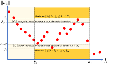
Figure 1: An example of a plausible sequence of iterates and the norms of their directions. Each red dot represents an iterate and its search direction norm. This illustrates Lemma 4.

Let

$$\mathcal{P}_{\epsilon}:=\{k\in\mathbf{N}:\hat{\rho}_{k}\geq\beta,\underaccent{\bar}{k}_{\epsilon}\leq k<K_{\epsilon}\}$$

which represents the set of iterations, before we find an $\epsilon$-approximate stationary point, where the function value is reduced a large amount compared with our target reduction, i.e., $\hat{\rho}_{k}\geq\beta$. Lemma 5 shows that there is a finite number of these iterations until the gradient drops below the target threshold $\epsilon$. The proof of Lemma 5 appears in Appendix A.2. Roughly, the idea of the proof is to use that, due our definition of $\hat{\rho}_{k}$, when $\hat{\rho}_{k}\geq\beta$ we always reduce the function value by at least $\frac{\beta\theta}{2}\|\gradient f(x_{k}+d_{k})\|\|d_{k}\|$ and $\|d_{k}\|$ can be lower bounded by $\underaccent{\bar}{d}_{\epsilon}$ using Lemma 4. As we cannot reduce the function value by a constant value indefinitely, we must eventually have $\|\gradient f(x_{k}+d_{k})\|\leq\epsilon$.

Lemma 5.

Suppose $\gradient^{2}f$ is $L$-Lipschitz and $\epsilon\in(0,\infty)$ then $\absolutevalue{\mathcal{P}_{\epsilon}}\leq\frac{\bar{d}_{\epsilon}}{\underaccent{\bar}{d}_{\epsilon}\omega}+1=\frac{2\omega c_{1}^{1/2}}{\beta\theta}\cdot\frac{\Delta_{f}L^{1/2}}{\epsilon^{-3/2}}+1$.

With Lemma 5 in hand we are now ready to prove our main result, Theorem 1. We have already provided a bound on the length of the warm up period, $\underaccent{\bar}{k}_{\epsilon}$ (Lemma 4) and on the number of points with $\hat{\rho}_{k}\geq\beta$. Therefore, the only obstacle is to bound the number of points with $\hat{\rho}_{k}<\beta$. However, on these iterations we always decrease the radius by at least $\omega$ (see update rules in Algorithm 1), and therefore as $\|d_{k}\|$ is bounded below by $\underaccent{\bar}{d}_{\epsilon}$, there must be iterations where we increase the radius $r_{k}$, which by definition of Algorithm 1 only occurs if $\beta\geq\hat{\rho}_{k}$. Consequently, the number of iterations where $\beta<\hat{\rho}_{k}$ can be bounded by the number of iterations where $\beta\geq\hat{\rho}_{k}$ plus a $\tilde{O}(1)$ term. This is the crux of the proof of Theorem 1 which appears in Section A.3.

Theorem 1.

Suppose that $\gradient^{2}f$ is $L$-Lipschitz and $f$ is bounded below with $\Delta_{f}=f(x_{1})-f_{\star}$, then for all $\epsilon\in(0,\infty)$ there exists some iteration $k$ with $\|\gradient f(x_{k}+d_{k})\|\leq\epsilon$ and

$$k\leq O\left(\frac{\Delta_{f}L^{\frac{1}{2}}}{\epsilon^{\frac{3}{2}}}+\log\left(\frac{\epsilon^{\frac{1}{2}}}{L^{\frac{1}{2}}r_{1}}+\frac{r_{1}\epsilon}{\Delta_{f}}+1\right)+1\right)$$

where $O(\cdot)$ hides problem-independent constant factors and $r_{1}$ is the initial trust-region radius.

One drawback of Theorem 1 is that it only bounds the number of iterations to find a first-order stationary point. Many second-order methods in the literature show convergence to points satisfying the second-order optimality conditions [47, 35, 36, 18]. Of course, these methods are not consistently adaptive. Therefore, in the future, it would be interesting to develop a method that provides a consistently adaptive convergence guarantee for finding second-order stationary points.

4 Quadratic convergence when sufficient conditions for local optimality hold

Theorem 2.

Suppose $f$ is twice differentiable and for some $x_{\star}\in R^{n}$ the second-order sufficient conditions for local optimality hold ($\gradient f(x_{\star})=0$ and $\gradient^{2}f(x_{\star})\succ 0$). Under these conditions there exists a neighborhood $N$ around $x_{\star}$ and a constant $c>0$ such that if $x_{i}\in N$ then there exist $x_{\hat{k}}\in N$ such that for all $k\geq\hat{k}$ we have $\|x_{k+1}-x_{\star}\|\leq c\|x_{k}-x_{\star}\|^{2}\leq\frac{1}{2}\|x_{k}-x_{\star}\|$.

The proof of Theorem 2 appears in Section B. It is a little tricker than typical quadratic convergence proofs for trust-region methods because in our method we have $\lim_{k\rightarrow 0}r_{k}\rightarrow 0$ whereas classical trust-region methods have $r_{k}$ bounded away from zero [22, Proof of Theorem 4.14]. Fortunately, one can show that asymptotically $r_{k}\geq\omega\|x_{k}-x_{\star}\|$ so the decaying radius does not interfere with quadratic convergence. In particular, the crux of proving Theorem 2 is proving the premise of Lemma 6 (as the conclusion of Lemma 6 is $r_{k}\geq\omega\|x_{k}-x_{\star}\|$). For this Lemma we define $\mathbf{diam}(X):=\sup_{x,x^{\prime}\in X}\|x-x^{\prime}\|$.

Lemma 6.

Let $N$ be a bounded set such that for all $x_{k}\in N$ we have $x_{k+1}\in N$, $\hat{\rho}_{k}\geq\beta$, and $\min\{\gamma_{2}r_{k},\|x_{k+1}-x_{\star}\|\}\leq\|d_{k}\|\leq\omega\gamma_{2}\|x_{k}-x_{\star}\|$. Suppose there exists $x_{k}\in N$ and let $i$ be the smallest index with $x_{i}\in N$, then $r_{k}\geq\omega\|x_{k}-x_{\star}\|$ for all $k\geq 2+i+\log_{\gamma_{2}\omega}(\frac{\mathbf{diam}(N)}{\|d_{i}\|})$.

Proof.

Let $k\geq i$. By induction $x_{k}\in N$. By $\hat{\rho}_{k}\geq\beta$ and inspection of Algorithm 1 we have $r_{k+1}=\omega\|d_{k}\|$. Suppose that $\|d_{k}\|\geq\gamma_{2}r_{k}$ for all $i\leq k\leq i+\ell$ then $\mathbf{diam}(N)\geq\|d_{k+1}\|\geq\gamma_{2}r_{k+1}=\gamma_{2}\omega\|d_{k}\|=\gamma_{2}^{\ell}\omega^{\ell}\|d_{i}\|$. Rearranging gives $\ell\leq\log_{\gamma_{2}\omega}(\frac{\mathbf{diam}(N)}{\|d_{i}\|})$. Next observe that if $\|d_{k}\|<\gamma_{2}r_{k}$ then $\|d_{k+1}\|\leq\omega\gamma_{2}\|x_{k+1}-x_{\star}\|\leq\omega\gamma_{2}\|d_{k}\|=(\omega\gamma_{2}/\omega)r_{k+1}=r_{k+1}$. By induction $\|d_{k}\|<\gamma_{2}r_{k}$ for all $k>\ell$. Finally, observe that if $\|d_{k}\|<\gamma_{2}r_{k}$ then $r_{k+1}=\omega\|d_{k}\|\geq\omega\|x_{k+1}-x_{\star}\|$. ∎

5 Experimental results

We test our algorithm on learning linear dynamical systems [48], matrix completion [49], and the CUTEst test set [50].

Appendix D contains the complete set of results from our experiments. Our method is implemented in an open-source Julia module available at https://github.com/fadihamad94/CAT-NeurIPS. The implementation uses a factorization and eigendecomposition approach to solve the trust-region subproblems (i.e., satisfy (6)). We perform our experiments using Julia 1.6 on a Linux virtual machine that has 8 CPUs and 16 GB RAM. The CAT code repository provides instructions for reproducing the experiments and detailed tables of results.

For these experiments, the selection of the parameters (unless otherwise specified) is as follow: $r_{1}=1.0$, $\beta=0.1$, $\theta=0.1$, $\omega=8.0$, $\gamma_{1}=0.0$, $\gamma_{2}=0.8$, and $\gamma_{3}=1.0$. When implementing Algorithm 1 with some target tolerance $\epsilon$, we immediately terminate when we observe a point $x_{k}$ with $\|\gradient f(x_{k}+d_{k})\|\leq\epsilon$. This also includes the case when we check the inner termination criteria for the trust-region subproblem. The full details of the implementation are described in Appendix C.

5.1 Learning linear dynamical systems

We test our method on learning linear dynamical systems [48] to see how efficient our method compared to a trust-region solver. We synthetically generate an example with noise both in the observations and also the evolution of the system, and then recover the parameters using maximum likelihood estimation. Details are provided in Appendix D.1.

On this problem we compare our algorithm with a Newton trust-region method that is available through the Optim.jl package [51]. The comparisons are summarized in Table 2.

Table 2: Geometric mean for total number of iterations, and evaluations of the function and gradient, per solver on 60 randomly generated instances with $\epsilon=10^{-5}$ termination tolerance. Failures counted as the maximum number of iterations ($10000$) when computing the geometric mean.

	#iter	#function	#gradient
Newton trust-region [51]	480.1	482.3	482.3
Our method	308.1	309.6	309.6
$95\%$ CI for ratio	[1.24, 1.95]	[1.24, 1.94]	[1.24, 1.94]

5.2 Matrix completion

We also demonstrate the effectiveness of our algorithm against a trust-region solver on the matrix completion problem. The matrix completion formulation can be written as the regularized squared error function of SVD model [49, Equation 10]. For our experiment, we use the public data set of Ausgrid, but we only use the data from a single substation. Details are provided in Appendix D.2.

Again we compare our algorithm with a Newton trust-region method [51]. The comparison are summarized in Table 3.

Table 3: Geometric mean for total number of iterations per solver on 10 instances by randomly generating the sampled measurements from the matrix D using data from Ausgrid with $\epsilon=10^{-5}$ termination tolerance. Failures counted as the maximum number of iterations ($1000$) when computing the geometric mean.

	#iter
Newton trust-region [51]	1000
Our method	216.4

5.3 Results on CUTEst test set

The CUTEst test set [50] is a standard test set for nonlinear optimization algorithms. To run the benchmarks we use https://github.com/JuliaSmoothOptimizers/CUTEst.jl (the License can be found at https://github.com/JuliaSmoothOptimizers/CUTEst.jl/blob/main/LICENSE.md). We will be comparing with the results for ARC reported in [52, Table 1]. As the benchmark CUTEst that we used has changed since [52] was written we select only the problems in CUTEst that remain the same (some of the problem sizes have changed). This gives 67 instances. A table with our full results can be found in the results/CUTEst subdirectory in the git repository for this paper. Catris et.al [52] report the results for three different implementations of their ARC algorithm. We limit our comparison to the ARC g-rule algorithm since it performs better than the other ARC approaches. We also run the Newton trust-region method from the Optim.jl package [51].

Our algorithm is stopped as soon $\|\gradient f(x_{k}+d_{k})\|$ is smaller than $10^{-5}$. For the Newton trust-region method [51] we also used as a stopping criteria a value of $10^{-5}$ for the gradient termination tolerance. We used $10000$ as an iteration limit and any run exceeding this is considered a failure. This choice of parameters is to be consistent with [52].

As we can see from Table 4, our algorithm offers significant promise, requiring similar function evaluations (and therefore subproblem solves) to converge than the Newton trust-region of [51] and ARC, although the number of gradient evaluations is slightly higher than ARC. In addition, the comparison between these algorithms in term of total number of iterations and total number of gradient evaluations is summarized in Figure 2.

Table 4: Number of failures, geometric mean for total number of iterations and function and gradient evaluations per solver on 67 unconstrained instance from the CUTEst benchmark instances. Failures counted as the maximum number of iterations ($10000$) when computing the geometric mean.

	#failures	#iter	#function	#gradient
Our method	3	41.5	44.4	44.4
ARC with the g-rule [52]	1	38.1	38.1	26.6
Newton trust-region [51]	4	44.5	47.2	47.2

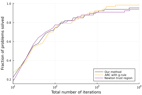
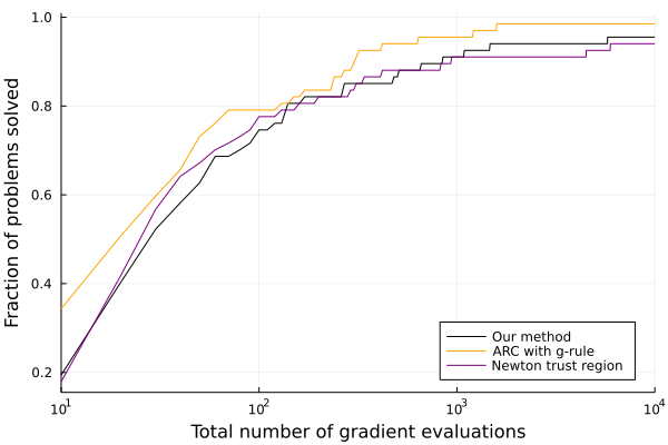
Figure 2: Fraction of problems solved on the CUTEst benchmark.

5.4 Convergence of our method with different theta values

To demonstrate the role of the additional $\frac{\theta}{2}\|d_{k}\|\|\gradient f(x_{k}+d_{k})\|$ term we run experiments with different $\theta$ values. In particular, we contrast our default value of $\theta=0.1$ with $\theta=0$ which corresponds to not adding the $\frac{\theta}{2}\|d_{k}\|\|\gradient f(x_{k}+d_{k})\|$ term to $\hat{\rho}_{k}$ (recall the discussion in Section 2.2).

In Figure 3(a) we rerun on the CUTEst test set (as per Section 5.3) and compare these two options. One can see the algorithm performs similarly with either $\theta=0$ or $\theta=0.1$.

In Figure 3(b) we test on the hard example from [45] which is designed to exhibit the poor worst-case complexity of trust-region methods (i.e., a convergence rate proportional to $\epsilon^{-2}$) if the initial radius $r_{1}$ is chosen sufficiently large (to achieve this we set $r_{1}=1.5$). We run this example with $\epsilon=10^{-3}$. One can see that while for the first $\approx 10^{4}$ iterations the methods follow identical trajectories, thereafter $\theta=0.1$ rapidly finds a stationary point whereas $\theta=0.0$ requires two orders of magnitude more iterations to terminate. This crystallizes the importance of $\theta$ in circumventing the worst-case $\epsilon^{-2}$ convergence rate of trust-region methods.

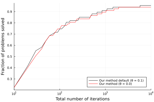
(a) Fraction of problems solved versus total number of iterations on the CUTEst test set

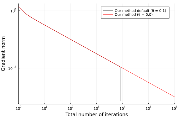
(b) Gradient norm versus total number of iterations on the example of [45] with $r_{1}=1.5$

Figure 3: Performance of our algorithm based on different $\theta$ values.

Checklist

1. For all authors…

   1. Do the main claims made in the abstract and introduction accurately reflect the paper’s contributions and scope? [Yes]

   2. Did you describe the limitations of your work? [Yes] The comparisons with other algorithms show the limitations of our work.

   3. Did you discuss any potential negative societal impacts of your work? [N/A]

   4. Have you read the ethics review guidelines and ensured that your paper conforms to them? [Yes]

2. If you are including theoretical results…

   1. Did you state the full set of assumptions of all theoretical results? [Yes] See Sections 3 and 4

   2. Did you include complete proofs of all theoretical results? [Yes] See Sections 3 and 4

3. If you ran experiments…

   1. Did you include the code, data, and instructions needed to reproduce the main experimental results (either in the supplemental material or as a URL)? [Yes] Code and instructions to reproduce the results are attached in the supplementary materials.

   2. Did you specify all the training details (e.g., data splits, hyperparameters, how they were chosen)? [N/A]

   3. Did you report error bars (e.g., with respect to the random seed after running experiments multiple times)? [Yes]

   4. Did you include the total amount of compute and the type of resources used (e.g., type of GPUs, internal cluster, or cloud provider)? [N/A]

4. If you are using existing assets (e.g., code, data, models) or curating/releasing new assets…

   1. If your work uses existing assets, did you cite the creators? [Yes] We use CUTEst.jl and Optim.jl. For both we cite the creators.

   2. Did you mention the license of the assets? [Yes] See Section 5.3 and Appendix D.1.

   3. Did you include any new assets either in the supplemental material or as a URL? [Yes] Our code is attached in the supplementary materials.

   4. Did you discuss whether and how consent was obtained from people whose data you’re using/curating? [No]

   5. Did you discuss whether the data you are using/curating contains personally identifiable information or offensive content? [N/A]

5. If you used crowdsourcing or conducted research with human subjects…

   1. Did you include the full text of instructions given to participants and screenshots, if applicable? [N/A]

   2. Did you describe any potential participant risks, with links to Institutional Review Board (IRB) approvals, if applicable? [N/A]

   3. Did you include the estimated hourly wage paid to participants and the total amount spent on participant compensation? [N/A]

Appendix A Proof of results from Section 3

A.1 Proof of Lemma 2

Proof.

First we prove result in the case that $\|d_{k}\|<\gamma_{2}r_{k}$. By (6b) the statement $\|d_{k}\|<\gamma_{2}r_{k}$ implies $\delta_{k}=0$. Combining $\delta_{k}=0$ with (6a) and (9) and using the fact $1-\gamma_{1}>0$ yields

$$\|\gradient f(x_{k}+d_{k})\|\leq\frac{L}{2(1-\gamma_{1})}\|d_{k}\|^{2}\leq c_{1}L\|d_{k}\|^{2}\ .$$

Next we prove the result in the case that $\hat{\rho}_{k}\leq\beta$. Then

$$M_{k}(d_{k})+\frac{L}{6}\|d_{k}\|^{3} \geq f(x_{k}+d_{k})-f(x_{k})=-\hat{\rho}_{k}\left(-M_{k}(d_{k})+\frac{\theta}{2}\|\gradient f(x_{k}+d_{k})\|\|d_{k}\|\right)$$

$$\geq-\beta\left(-M_{k}(d_{k})+\frac{\theta}{2}\|\gradient f(x_{k}+d_{k})\|\|d_{k}\|\right)$$

where the the first inequality uses (10), the first equality uses the definition of $\hat{\rho}_{k}$, and the second inequality uses $\hat{\rho}_{k}\leq\beta$ and $-M_{k}(d_{k})+\frac{\theta}{2}\|\gradient f(x_{k}+d_{k})\|\|d_{k}\|\geq 0$.

Rearranging the previous inequality using $1-\beta>0$ and then applying (6d) yields:

$$\frac{L}{3(1-\beta)}\|d_{k}\|^{2}+\frac{\beta\theta}{1-\beta}\|\gradient f(x_{k}+d_{k})\|\geq-\frac{2M_{k}(d_{k})}{\|d_{k}\|}\geq\gamma_{3}\delta_{k}\|d_{k}\|.$$ (13)

Now, by (9), (6a) and the triangle inequality, and (13) respectively:

$$\|\gradient f(x_{k}+d_{k})\| \leq\|\gradient M_{k}(d_{k})\|+\frac{L}{2}\|d_{k}\|^{2}\leq\delta_{k}\|d_{k}\|+\gamma_{1}\|\gradient f(x_{k}+d_{k})\|+\frac{L}{2}\|d_{k}\|^{2}$$

$$\leq L\left(\frac{1}{3\gamma_{3}(1-\beta)}+\frac{1}{2}\right)\|d_{k}\|^{2}+\left(\frac{\beta\theta}{\gamma_{3}(1-\beta)}+\gamma_{1}\right)\|\gradient f(x_{k}+d_{k})\|.$$

Rearranging the latter inequality for $\|\gradient f(x_{k}+d_{k})\|$ and using $\frac{\beta\theta}{\gamma_{3}(1-\beta)}+\gamma_{1}<1$ from the requirements of Algorithm 1 yields:

$$\|\gradient f(x_{k}+d_{k})\| \leq\frac{\frac{1}{3\gamma_{3}(1-\beta)}+\frac{1}{2}}{1-\frac{\beta\theta}{\gamma_{3}(1-\beta)}-\gamma_{1}}L\|d_{k}\|^{2}=\frac{2+3\gamma_{3}(1-\beta)}{6(\gamma_{3}(1-\gamma_{1})(1-\beta)-\beta\theta)}L\|d_{k}\|^{2}$$

$$\leq\frac{5-3\beta}{6(\gamma_{3}(1-\gamma_{1})(1-\beta)-\beta\theta)}L\|d_{k}\|^{2}.$$

∎

A.2 Proof of Lemma 5

Proof.

For conciseness let $m=\absolutevalue{\mathcal{P}_{\epsilon}}$. Suppose that the indices of $\mathcal{P}_{\epsilon}$ are ordered increasing value by a permutation function $\pi$, i.e., $\mathcal{P}_{\epsilon}=\{\pi(i):i\in[m]\}$ with $\pi(1)<\dots<\pi(m)$. Then

$$\Delta_{f} \geq f(x_{\pi(1)})-f(x_{\pi(m)})=\sum_{i=1}^{m-1}f(x_{\pi(i)})-f(x_{\pi(i+1)})$$

where the first inequality uses the fact that $f(x_{\pi(i)})$ is non-increasing in $\pi(i)$ and $f(x_{\pi(i)})\geq f_{\star}$ and the equality is simply the definition of the telescoping sum of $f(x_{\pi(m)})-f(x_{\pi(1)})$. Therefore,

$$\Delta_{f} \geq\sum_{i=1}^{m-1}f(x_{\pi(i)})-f(x_{\pi(i+1)})=\sum_{i=1}^{m-1}\hat{\rho}_{\pi(i)}\left(-M_{k}({d_{\pi(i)}})+\frac{\theta}{2}\|\gradient f(x_{\pi(i)}+d_{\pi(i)})\|\|d_{\pi(i)}\|\right)$$

$$\geq\sum_{i=1}^{m-1}\beta\left(-M_{k}(d_{\pi(i)})+\frac{\theta}{2}\|\gradient f(x_{\pi(i)}+d_{\pi(i)})\|\|d_{\pi(i)}\|\right)\geq\frac{\beta\theta}{2}\sum_{i=1}^{m-1}\|\gradient f(x_{\pi(i)}+d_{\pi(i)})\|\|d_{\pi(i)}\|$$

$$\geq\frac{\epsilon\beta\theta}{2}(m-1)\underaccent{\bar}{d}_{\epsilon}$$

where the first equality uses the definition of $\hat{\rho}_{\pi(i)}$, the second inequality follows from $\hat{\rho}_{\pi(i)}\geq\beta$ for $\pi(i)\in\mathcal{P}_{\epsilon}$, the third inequality uses that $-M_{k}(d_{\pi(i)})\geq 0$, the final inequality uses that $\pi(i)\in\mathcal{P}_{\epsilon}$ implies that $\|\gradient f(x_{\pi(i)}+d_{\pi(i)})\|\geq\epsilon$ (by definition of $\pi(i)\in\mathcal{P}_{\epsilon}$) and $\underaccent{\bar}{d}_{\epsilon}\leq\|d_{\pi(i)}\|$ (due to Lemma 4).

Rearranging the latter inequality for $m$ using the fact that $\beta\theta\epsilon\underaccent{\bar}{d}_{\epsilon}>0$ and $\Delta_{f}\geq 0$ yields $m\leq\frac{2\Delta_{f}}{\beta\theta\epsilon\underaccent{\bar}{d}_{\epsilon}}+1=\frac{\bar{d}_{\epsilon}}{\underaccent{\bar}{d}_{\epsilon}\omega}+1=$ where the equalities use the definitions of $\bar{d}_{\epsilon}$ and $\underaccent{\bar}{d}_{\epsilon}$. ∎

A.3 Proof of Theorem 1

Proof.

Define:

$$n_{j} :=\absolutevalue{\{k\in\mathbf{N}:k\not\in\mathcal{P}_{\epsilon},k<K_{\epsilon},\underaccent{\bar}{k}_{\epsilon}<k\leq j\}}$$

$$p_{j} :=\absolutevalue{\{k\in\mathcal{P}_{\epsilon}:\underaccent{\bar}{k}_{\epsilon}<k\leq j\}}.$$

First we establish that

$$n_{\infty}\leq p_{\infty}+\log_{\omega}\left(\max\left\{\frac{\bar{d}_{\epsilon}}{\underaccent{\bar}{d}_{\epsilon}},1\right\}\right).$$ (14)

Consider the induction hypothesis that

$$r_{k}\leq r_{\underaccent{\bar}{k}_{\epsilon}}\omega^{p_{k}-n_{k}}\quad\forall k\in[\underaccent{\bar}{k}_{\epsilon},K_{\epsilon})\cap\mathbf{N}.$$ (15)

If $k=\underaccent{\bar}{k}_{\epsilon}$ then $p_{k}=n_{k}=0$ and the hypothesis holds. Suppose that the induction hypothesis holds for $k=j$. Note that for all $j\in\mathbf{N}$ either $p_{j+1}=p_{j}+1$ (and $n_{j+1}=n_{j}$) or $n_{j+1}=n_{j}+1$ (and $p_{j+1}=p_{j}$). If $p_{j+1}=p_{j}+1$ then

$$r_{j+1}=\|d_{j}\|\omega\leq r_{j}\omega\leq r_{\underaccent{\bar}{k}_{\epsilon}}\omega^{p_{j}-n_{j}+1}=r_{\underaccent{\bar}{k}_{\epsilon}}\omega^{p_{j+1}-n_{j+1}}.$$

On the other hand, if $n_{j+1}=n_{j}+1$ then

$$r_{j+1}=\|d_{j}\|/\omega\leq r_{j}/\omega\leq r_{\underaccent{\bar}{k}_{\epsilon}}\omega^{p_{j}-n_{j}-1}=r_{\underaccent{\bar}{k}_{\epsilon}}\omega^{p_{j+1}-n_{j+1}}.$$

Therefore by induction (15) holds. By (15) and Lemma 4,

$$\underaccent{\bar}{d}_{\epsilon}\leq\bar{d}_{\epsilon}\omega^{p_{k}-n_{k}}$$

which establishes (14).

By Lemma 4 we have $\underaccent{\bar}{k}_{\epsilon}\leq 1+\log_{\gamma_{2}\omega}(\max\{1,\underaccent{\bar}{d}_{\epsilon}/r_{1},r_{1}/\bar{d}_{\epsilon}\})$ and Lemma 5 we have $p_{\infty}\leq\frac{\bar{d}_{\epsilon}}{\underaccent{\bar}{d}_{\epsilon}\omega}+1$; using these inequalities in conjuction with (14) gives

$$K_{\epsilon} =\underaccent{\bar}{k}_{\epsilon}+p_{\infty}+n_{\infty}+1\leq\underaccent{\bar}{k}_{\epsilon}+2p_{\infty}+\log_{\omega}\left(\max\{\bar{d}_{\epsilon}/\underaccent{\bar}{d}_{\epsilon}\}\right)+1$$

$$\leq\log_{\omega\gamma_{2}}(\max\{1,\underaccent{\bar}{d}_{\epsilon}/r_{1},r_{1}/\bar{d}_{\epsilon}\})+\frac{2\bar{d}_{\epsilon}}{\underaccent{\bar}{d}_{\epsilon}\omega}+\log_{\omega}(\max\{1,\bar{d}_{\epsilon}/\underaccent{\bar}{d}_{\epsilon}\})+3$$

$$\leq\frac{2\bar{d}_{\epsilon}}{\underaccent{\bar}{d}_{\epsilon}\omega}+2\log_{\omega\gamma_{2}}\left(\max\left\{\frac{\bar{d}_{\epsilon}}{\underaccent{\bar}{d}_{\epsilon}},\frac{\underaccent{\bar}{d}_{\epsilon}}{r_{1}},\frac{r_{1}}{\bar{d}_{\epsilon}},1\right\}\right)+3$$

$$=c_{2}\cdot\frac{\Delta_{f}L^{1/2}}{\epsilon^{-3/2}}+2\log_{\omega\gamma_{2}}\left(\max\left\{\frac{c_{2}\omega}{2}\cdot\frac{\Delta_{f}L^{1/2}}{\epsilon^{3/2}},\frac{\gamma_{2}}{\omega c_{1}^{1/2}}\cdot\frac{\epsilon^{1/2}}{L^{1/2}r_{1}},\frac{\beta\theta}{2\omega}\cdot\frac{r_{1}L^{1/2}}{\epsilon^{1/2}},1\right\}\right)+3$$

where

$$c_{2}:=\frac{4c_{1}^{1/2}\omega}{\beta\theta\gamma_{2}}$$

is a problem-independent constant. As $c_{1},c_{2},\omega,\beta,\theta,\gamma_{1},\gamma_{2}$ and $\gamma_{3}$ are problem-independent constants (see the definition of $c_{1}$ in Lemma 2 and the requirements of Algorithm 1) the result follows. ∎

Appendix B Proof of Theorem 2

We first prove Theorem 3 and then reduce Theorem 2 to Theorem 3. The following fact will be useful.

Fact 3 ([53]).

If $f$ is $\alpha$-strongly convex and $S$-smooth on the set $C$ (i.e., $\alpha\mbox{\bf I}\preceq\gradient^{2}f(x)\preceq S\mbox{\bf I}$ for all $x\in C$) then

$$\alpha\|x-x_{\star}\|\leq\|\gradient f(x)\|\leq S\|x-x_{\star}\|$$ (16)

where $x_{\star}$ is any minimizer of $f$.

Theorem 3.

Suppose that $f$ is $L$-Lipschitz, $\gradient f(x_{\star})=0$ and there exists $\alpha,S,t>0$ such that $\alpha\mbox{\bf I}\preceq\gradient^{2}f(x)\preceq S\mbox{\bf I}$ for all $x\in\{x\in{\bf R}^{n}:\|x-x_{\star}\|\leq t\}$. Consider the set

$$C:=\left\{x\in{\bf R}^{n}:f(x)\leq f(x_{\star})+\frac{2\eta^{2}}{\alpha},\|x-x_{\star}\|\leq\eta\right\}$$

with

$$\eta=\min\left\{t,\frac{\alpha^{3}(1-\gamma_{1})}{2LS^{2}}\min\left\{\frac{1}{2},\omega\gamma_{2}-1\right\},\frac{3(1-\beta)\alpha}{\left(2+12(1-\beta)\gamma_{1}c_{1}\right)L\omega\gamma_{2}},\frac{(1-\beta)\alpha}{2\omega\gamma_{2}\beta\theta Lc_{1}}\right\}$$

then if $x_{i}\in C$ then for $k\geq 2+i+\log_{\gamma_{2}\omega}(\frac{\eta}{\|d_{i}\|})$ we have

$$\|x_{k+1}-x_{\star}\|\leq\frac{2LS^{2}}{\alpha^{3}(1-\gamma_{1})}\|x_{k}-x_{\star}\|^{2}.$$

Proof.

We begin by establishing the premise of Lemma 6. First we establish $x_{k}\in C\implies x_{k+1}\in C$. Suppose that $x_{k}\in C$ then $f(x_{k+1})\leq f(x_{k})\leq f(x_{\star})+\frac{2\eta^{2}}{\alpha}$. By strong convexity we get $x_{k+1}\in C$.

Next we establish that $\min\{\gamma_{2}r_{k},\|x_{k+1}-x_{\star}\|\}\leq\|d_{k}\|\leq\omega\gamma_{2}\|x_{k}-x_{\star}\|$. By strong convexity and (6d) we have

$$\frac{\alpha+\delta_{k}}{2}\|d_{k}\|^{2}-\|\gradient f(x_{k})\|\|d_{k}\|\leq M_{k}(d_{k})\leq 0$$

which implies $\|d_{k}\|\leq\frac{2\|\gradient f(x_{k})\|}{\alpha+\delta_{k}}$. Furthermore, by (9), (6a) and $\|d_{k}\|\leq\frac{2\|\gradient f(x_{k})\|}{\alpha+\delta_{k}}$ we have

$$\|\gradient f(x_{k}+d_{k})+\delta_{k}d_{k}\|\leq\|\gradient M_{k}(d_{k})+\delta_{k}d_{k}\|+\frac{L}{2}\|d_{k}\|^{2}\leq\gamma_{1}\|\gradient f(x_{k}+d_{k})\|+\frac{2L\|\gradient f(x_{k})\|^{2}}{\alpha^{2}}$$

which after rearranging

$$\|\gradient f(x_{k}+d_{k})+\delta_{k}d_{k}\|\leq\frac{2L}{\alpha^{2}(1-\gamma_{1})}\|\gradient f(x_{k})\|^{2}$$ (17)

By strong convexity and smoothness,

$$\|x_{k}+d_{k}-\hat{x}_{k}\|\leq\frac{2LS^{2}}{\alpha^{3}(1-\gamma_{1})}\|x_{k}-x_{\star}\|^{2}$$ (18)

where $\hat{x}_{k}:=\min f(x)+\frac{\delta_{k}}{2}\|x-x_{k}\|^{2}$. Therefore, as $\|x_{k}-x_{\star}\|\leq\frac{\alpha^{3}(1-\gamma_{1})}{2LS^{2}}\min\left\{\frac{1}{2},\omega\gamma_{2}-1\right\}$,

$$\|x_{k}+d_{k}-\hat{x}_{k}\|\leq\min\left\{\frac{1}{2},\omega\gamma_{2}-1\right\}\|x_{k}-x_{\star}\|$$

which combined with the triangle inequality and $\|\hat{x}_{k}-x_{k}\|\leq\|x_{k}-x_{\star}\|$ gives

$$\|d_{k}\|\leq\|x_{k}+d_{k}-\hat{x}_{k}\|+\|x_{k}-\hat{x}_{k}\|\leq\omega\gamma_{2}\|x_{k}-x_{\star}\|$$

Furthermore, if $\|d_{k}\|<\gamma_{2}r_{k}$ then by (6b) we have $\delta_{k}=0$ and $\hat{x}_{k}=x_{\star}$ which gives

$$\|x_{k}+d_{k}-x_{\star}\|\leq\frac{1}{2}\|x_{k}-x_{\star}\|\leq\|x_{k}-x_{\star}\|-\|x_{k}+d_{k}-x_{\star}\|\leq\|d_{k}\|.$$

Next we show $x_{k}\in C$ implies $\hat{\rho}_{k}\geq\beta$. To obtain a contradiction we assume $\hat{\rho}_{k}<\beta$, by the definition of the model, (6a), strong convexity, and (11) we get

$$M_{k}(d_{k}) =\frac{1}{2}d_{k}^{T}\gradient^{2}f(x_{k})d_{k}+\gradient f(x_{k})^{T}d_{k}=d_{k}^{T}(\gradient^{2}f(x_{k})d_{k}+\delta_{k}d_{k}+\gradient f(x_{k}))-\frac{1}{2}d_{k}^{T}(\gradient^{2}f(x_{k})+2\delta_{k}\mbox{\bf I})d_{k}$$

$$\leq\gamma_{1}\|d_{k}\|\|\gradient f(x_{k}+d_{k})\|-\frac{1}{2}d_{k}^{T}(\gradient^{2}f(x_{k})+2\delta_{k}\mbox{\bf I})d_{k}$$

$$\leq\gamma_{1}\|d_{k}\|\|\gradient f(x_{k}+d_{k})\|-\frac{\alpha}{2}\|d_{k}\|^{2}$$

$$\leq\gamma_{1}c_{1}L\|d_{k}\|^{3}-\frac{\alpha}{2}\|d_{k}\|^{2}.$$

It follows that by inequality (10), $\|d_{k}\|\leq\omega\gamma_{2}\|x_{k}-x_{\star}\|\leq\frac{3(1-\beta)\alpha}{\left(2+12(1-\beta)\gamma_{1}c_{1}\right)L}$, inequality (11), $\|d_{k}\|\leq\omega\gamma_{2}\|x_{k}-x_{\star}\|\leq\frac{(1-\beta)\alpha}{2\beta\theta Lc_{1}}$ we have

$$f(x_{k})-f(x_{k+1}) \geq-M_{k}(d_{k})-\frac{L}{6}\|d_{k}\|^{3}$$

$$\geq-\beta M_{k}(d_{k})+(\beta-1)M_{k}(d_{k})-\frac{L}{6}\|d_{k}\|^{3}$$

$$\geq-\beta M_{k}(d_{k})+\frac{(1-\beta)\alpha}{2}\|d_{k}\|^{2}+(\beta-1)\gamma_{1}c_{1}L\|d_{k}\|^{3}-\frac{L}{6}\|d_{k}\|^{3}$$

$$\geq-\beta M_{k}(d_{k})+\frac{(1-\beta)\alpha}{2}\|d_{k}\|^{2}-L\|d_{k}\|^{3}\left(\frac{1+6(1-\beta)\gamma_{1}c_{1}}{6}\right)$$

$$\geq-\beta M_{k}(d_{k})+\frac{(1-\beta)\alpha}{2}\|d_{k}\|^{2}-\frac{(1-\beta)\alpha}{4}\|d_{k}\|^{2}$$

$$\geq-\beta M_{k}(d_{k})+\frac{(1-\beta)\alpha}{4}\|d_{k}\|^{2}$$

$$\geq-\beta M_{k}(d_{k})+\frac{(1-\beta)\alpha}{4Lc_{1}}\|\gradient f(x_{k}+d_{k})\|$$

$$\geq\beta\left(-M_{k}(d_{k})+\frac{\theta}{2}\|\gradient f(x_{k}+d_{k})\|d_{k}\|\right)$$

which after rearranging gives:

$$\hat{\rho}_{k}=\frac{f(x_{k})-f(x_{k}+d_{k})}{-M_{k}(d_{k})+\frac{\theta}{2}\|\gradient f(x_{k}+d_{k})\|d_{k}\|}\geq\beta$$

which gives our desired contradiction.

With the premise of Lemma 6 established we conclude that for $k\geq 2+i+\log\left(\eta/\|d_{i}\|\right)$ we have $\delta_{k}=0$ and therefore by (18) we get the desired result. ∎

The following Lemma is a standard result but we include it for completeness.

Lemma 7.

If $\gradient^{2}f(x_{\star})$ is twice differentiable and positive definite, then there exists a neighborhood $N$ and positive constants $\alpha,\beta>0$ such that $\alpha\mbox{\bf I}\preceq\gradient^{2}f(x)\preceq S\mbox{\bf I}$ for all $x\in N$.

Proof.

As $\gradient^{2}f$ is twice differentiable and the fact that continuous functions on compact sets are bounded we conclude that there exists a neighborhood $N$ around $x_{\star}$ that $\gradient^{2}f$ is $L$-Lipschitz for some constant $L\in(0,\infty)$. Then by using the fact that there exists positive constants $\alpha^{\prime},\beta^{\prime}\in(0,\infty)$ s.t. $\alpha^{\prime}\mbox{\bf I}\preceq\gradient^{2}f(x_{\star})\preceq\beta^{\prime}\mbox{\bf I}$ we conclude for sufficiently small ball around $x_{\star}$ we have $\alpha^{\prime}/2\mbox{\bf I}\preceq\gradient^{2}f(x)\preceq 2\beta^{\prime}\mbox{\bf I}$ for all $x$ in a sufficiently small neighborhood $N^{\prime}\subseteq N$. ∎

Proof of Theorem 2.

Follows by Lemma 7 and Theorem 3. ∎

Appendix C Solving trust-region subproblem

In this section, we detail our approach to solve the trust-region subproblem. We first attempt to take a Newton’s step by checking if $\gradient^{2}f(x_{k})\succeq 0$ and $\|\gradient^{2}f(x_{k})^{-1}\gradient f(x_{k})\|\leq r_{k}$. However, if that is not the case, then the optimally conditions mentioned in (6), will be a key ingredient in our approach to find $\delta$ and hence $d_{k}(\delta)$. Based on these optimally conditions, we will define a univariate function $\phi$ that we seek to find its root at each iteration. In our implementation we use $\gamma_{3}=1.0$ for (6d) which is the same as satisfying (5d). The function $\phi$ is defined as bellow:

$$\phi(\delta):=\begin{cases}-1,&\text{if $\gradient^{2}f(x_{k})+\delta\mbox{\bf I}\nsucceq 0\text{ or }\|d_{k}(\delta)\|>r_{k}$}\\ +1,&\text{if $\gradient^{2}f(x_{k})+\delta\mbox{\bf I}\succeq 0\And\|d_{k}(\delta)\|<\gamma_{2}r_{k}$}\\ 0,&\text{if $\gradient^{2}f(x_{k})+\delta\mbox{\bf I}\succeq 0\And\|d_{k}(\delta)\|\leq r_{k}$}\end{cases}$$

where:

$$d_{k}(\delta):=(\gradient^{2}f(x_{k})+\delta\mbox{\bf I})^{-1}(-\gradient f(x_{k}))$$

When we fail to take a Newton’s step, we first find an interval $[\delta,\delta^{\prime}]$ such that $\phi(\delta)\times\phi(\delta^{\prime})\leq 0$. Then we apply bisection method to find $\delta_{k}$ such that $\phi(\delta_{k})=0$. In case our root finding logic failed,

then we use the approach from the hard case section under chapter 4 "Trust-Region Methods" in [44] to find the direction $d_{k}$.

The logic to find the interval $[\delta,\delta^{\prime}]$ is summarized as follow. We first compute $\phi(\delta)$ using the $\delta$ value from the previous iteration. Then we search for $\delta^{\prime}$ by starting with $\delta^{\prime}=2\delta$. We compute $\phi(\delta^{\prime})$ and in the case $\phi(\delta^{\prime})<0$, we update $\delta^{\prime}$ to become twice its current value, otherwise if $\phi(\delta^{\prime})>0$, we update $\delta^{\prime}$ to become half its current value. We keep repeating this logic until we get a $\delta^{\prime}$ such that $\phi(\delta)\times\phi(\delta^{\prime})\leq 0$ or until we reach the maximum iteration limit which is marked as a failure.

The whole approach is summarized in Algorithm 2:

if $\gradient^{2}f(x_{k})\succeq 0$ then

       $d_{k}=-\gradient^{2}f(x_{k})^{-1}\gradient f(x_{k})$

      if $\|d_{k}\|\leq r$ then

             return $d_{k}$;

            

      

if hard case then

       Find $d_{k}$ using [44, pages 87-88] ;

      

      return $d_{k}$

else

       Find initial interval $[\delta,\delta^{\prime}]$ using the $\phi$ function such that $\phi(\delta)\times\phi(\delta^{\prime})\leq 0$ ;

      

      Use bisection method to find $\delta_{k}$ such that $\phi(\delta_{k})=0$ ;

      

      return $d_{k}(\delta_{k})$

Algorithm 2 trust-region subproblems solver

Appendix D Experimental results details

D.1 Learning linear dynamical systems

The time-invariant linear dynamical system is defined by:

$$h_{t+1} =Ah_{t}+Bu_{t}+\xi_{t}$$

$$x_{t} =h_{t}+\vartheta_{t}$$

where the vectors $h_{t}$ and $x_{t}$ represent the hidden and observed state of the system at time $t$. Here $u_{t},\vartheta_{t}\sim N(0,1)^{d}$,

$\xi_{t}\sim N(0,\sigma)^{d}$ and $A\text{ and }B$ are linear transformations.

The goal is to recover the parameters of the system using maximum likelihood estimation and hence we formulate the problem as follow:

$$\min_{A,B,h}\sum_{t=1}^{T}\frac{\|h_{t+1}-Ah_{t}-Bu_{t}\|^{2}}{\sigma^{2}}+\|x_{t}-h_{t}\|^{2}$$

We synthetically generate examples with noise both in the observations and also the evolution of the system. The entries of the matrix $B$ are generated using a Normal distribution $N(0,1)$. For the matrix $A$, we first generate a diagonal matrix $D$ with entries drawn from a uniform distribution $U[0.9,0.99]$ and then we construct a random orthogonal matrix $Q$ by randomly sampling a matrix $W\sim N(0,1)^{d\times d}$ and then performing an QR factorization. Finally using the matrices $Q$ and $D$, we define $A$:

$$A=Q^{T}DQ$$

We compare our method against the Newton trust-region method available through the Optim.jl package [51] licensed under https://github.com/JuliaNLSolvers/Optim.jl/blob/master/LICENSE.md. In the results/learning problem subdirectory in the git repository,

we present the full results of running our experiments on 60 randomly generated instances with $T=50$, $d=4$, and $\sigma=0.01$ where we used a value of $10^{-5}$ for the gradient termination tolerance.

This experiment was performed on a MacBook Air (M1, 2020) with 8GB RAM.

D.2 Matrix completion

The original power consumption data is denoted by a matrix $D\in R^{n_{1}\times n_{2}}$ where $n_{1}$ represents the number of measurements taken per day within a 15 mins interval and $n_{2}$ represents the number of days. Part of the data is missing, hence the goal is to recover the original data. The set $\Omega=\{(i,j)|D_{i,j}\text{ is observed}\}$ denotes the indices of the observed data in the matrix $D$.

We decompose $D$ as a product of two matrices $P\in R^{n_{1}\times r}$ and $Q\in R^{n_{2}\times r}$ where $r<n_{1}$ and $r<n_{2}$:

$$D=PQ^{T}.$$

To account for the effect of time and day on the power consumption data , we use a baseline estimate [54]:

$$d_{i,j}=\mu+r_{i}+c_{j}$$

where $\mu$ denotes the mean for all observed measurements, $r_{i}$ denotes the observed deviation during time $i$, and $c_{j}$ denotes the observed deviation during day $j$ [49, 54].

We formulate the matrix completion problem as the regularized squared error function of SVD model [49, Equation 10]:

$$\min_{r,c,p,q}\sum_{(i,j)\in\Omega}(D_{i,j}-\mu-r_{i}-c_{j}-p_{i}q_{j}^{T})+\lambda_{1}(r_{i}^{2}+c_{j}^{2})+\lambda_{2}(\|p_{i}\|_{2}^{2}+\|q_{j}\|_{2}^{2})$$

We use the public data set of Ausgrid, but we only use the data from a single substation (the Newton trust-region method [51] is very slow for this example so testing it on all substations takes a prohibitively long time). We limit our option to 30 days and 12 hours measurements i.e the matrix D is of size $48\times 30$ because with a larger matrix size, the Newton trust-region [51] was always reaching the iterations limit.

We compare our method against Newton trust-region algorithm available through the Optim.jl package [51] licensed under https://github.com/JuliaNLSolvers/Optim.jl/blob/master/LICENSE.md. In the results/matrix completion subdirectory in the git repository,

we include the full results of running our experiments on 10 instances by randomly generating the sampled measurements from the matrix $D$ with the same values for the regularization parameters as in [49] where we used a value of $10^{-5}$ for the gradient termination tolerance.

This experiment was performed on a MacBook Air (M1, 2020) with 8GB RAM.

References

• [1] John T Betts. Practical methods for optimal control and estimation using nonlinear programming. SIAM, 2010.
• [2] Klaus Schittkowski, Christian Zillober, and Rainer Zotemantel. Numerical comparison of nonlinear programming algorithms for structural optimization. Structural Optimization, 7(1):1–19, 1994.
• [3] Stephen Frank, Steffen Rebennack, et al. A primer on optimal power flow: Theory, formulation, and practical examples. Colorado School of Mines, Tech. Rep, 2012.
• [4] Lorenz T Biegler, Omar Ghattas, Matthias Heinkenschloss, and Bart van Bloemen Waanders. Large-scale PDE-constrained optimization: an introduction. In Large-Scale PDE-Constrained Optimization, pages 3–13. Springer, 2003.
• [5] Jonas Moritz Kohler and Aurelien Lucchi. Sub-sampled cubic regularization for non-convex optimization. In International Conference on Machine Learning, pages 1895–1904. PMLR, 2017.
• [6] Dongruo Zhou, Pan Xu, and Quanquan Gu. Stochastic variance-reduced cubic regularized Newton methods. In International Conference on Machine Learning, pages 5990–5999. PMLR, 2018.
• [7] Ching-pei Lee, Cong Han Lim, and Stephen J Wright. A distributed quasi-Newton algorithm for empirical risk minimization with nonsmooth regularization. In Proceedings of the 24th ACM SIGKDD International Conference on Knowledge Discovery & Data Mining, pages 1646–1655, 2018.
• [8] Frank E Curtis, Michael J O’Neill, and Daniel P Robinson. Worst-case complexity of an SQP method for nonlinear equality constrained stochastic optimization. arXiv preprint arXiv:2112.14799, 2021.
• [9] Frank E Curtis and Rui Shi. A fully stochastic second-order trust region method. Optimization Methods and Software, pages 1–34, 2020.
• [10] Frank E Curtis, Katya Scheinberg, and Rui Shi. A stochastic trust region algorithm based on careful step normalization. Informs Journal on Optimization, 1(3):200–220, 2019.
• [11] Vipul Gupta, Avishek Ghosh, Michał Dereziński, Rajiv Khanna, Kannan Ramchandran, and Michael W Mahoney. LocalNewton: Reducing communication rounds for distributed learning. In Uncertainty in Artificial Intelligence, pages 632–642. PMLR, 2021.
• [12] Peng Xu, Fred Roosta, and Michael W Mahoney. Newton-type methods for non-convex optimization under inexact Hessian information. Mathematical Programming, 184(1):35–70, 2020.
• [13] Chih-Hao Fang, Sudhir B Kylasa, Fred Roosta, Michael W Mahoney, and Ananth Grama. Newton-ADMM: A distributed GPU-accelerated optimizer for multiclass classification problems. In SC20: International Conference for High Performance Computing, Networking, Storage and Analysis, pages 1–12. IEEE, 2020.
• [14] Shusen Wang, Fred Roosta, Peng Xu, and Michael W Mahoney. Giant: Globally improved approximate Newton method for distributed optimization. Advances in Neural Information Processing Systems, 31, 2018.
• [15] Sen Na, Michał Dereziński, and Michael W Mahoney. Hessian averaging in stochastic Newton methods achieves superlinear convergence. arXiv preprint arXiv:2204.09266, 2022.
• [16] Peng Xu, Jiyan Yang, Fred Roosta, Christopher Ré, and Michael W Mahoney. Sub-sampled Newton methods with non-uniform sampling. Advances in Neural Information Processing Systems, 29, 2016.
• [17] Rixon Crane and Fred Roosta. DINO: Distributed Newton-type optimization method. In International Conference on Machine Learning, pages 2174–2184. PMLR, 2020.
• [18] Junyu Zhang, Lin Xiao, and Shuzhong Zhang. Adaptive stochastic variance reduction for subsampled Newton method with cubic regularization. INFORMS Journal on Optimization, 4(1):45–64, 2022.
• [19] Dmitry Kovalev, Konstantin Mishchenko, and Peter Richtárik. Stochastic Newton and cubic Newton methods with simple local linear-quadratic rates. arXiv preprint arXiv:1912.01597, 2019.
• [20] Philip E Gill and Walter Murray. Newton-type methods for unconstrained and linearly constrained optimization. Mathematical Programming, 7(1):311–350, 1974.
• [21] Jorge J Moré and Danny C Sorensen. On the use of directions of negative curvature in a modified Newton method. Mathematical Programming, 16(1):1–20, 1979.
• [22] Danny C Sorensen. Newton’s method with a model trust region modification. SIAM Journal on Numerical Analysis, 19(2):409–426, 1982.
• [23] Stefan Ulbrich. On the superlinear local convergence of a filter-SQP method. Mathematical Programming, 100(1):217–245, 2004.
• [24] Luís N Vicente and Stephen J Wright. Local convergence of a primal-dual method for degenerate nonlinear programming. Computational Optimization and Applications, 22(3):311–328, 2002.
• [25] Richard H Byrd, Jean Charles Gilbert, and Jorge Nocedal. A trust region method based on interior point techniques for nonlinear programming. Mathematical Programming, 89(1):149–185, 2000.
• [26] Lifeng Chen and Donald Goldfarb. Interior-point $l_{2}$-penalty methods for nonlinear programming with strong global convergence properties. Mathematical Programming, 108(1):1–36, 2006.
• [27] Andrew R Conn, Nicholas IM Gould, Dominique Orban, and Philippe L Toint. A primal-dual trust-region algorithm for non-convex nonlinear programming. Mathematical programming, 87(2):215–249, 2000.
• [28] Nicholas IM Gould, Dominique Orban, and Philippe L Toint. An interior-point $\ell_{1}$-penalty method for nonlinear optimization. Citeseer, 2002.
• [29] Andreas Wächter and Lorenz T Biegler. Line search filter methods for nonlinear programming: Motivation and global convergence. SIAM Journal on Optimization, 16(1):1–31, 2005.
• [30] Stephen Wright and Jorge Nocedal. Numerical optimization. Springer Science and Media, 2006.
• [31] Yurii Nesterov and Boris T Polyak. Cubic regularization of Newton method and its global performance. Mathematical Programming, 108(1):177–205, 2006.
• [32] Yair Carmon, John C Duchi, Oliver Hinder, and Aaron Sidford. Lower bounds for finding stationary points I. Mathematical Programming, 2020.
• [33] Geovani Nunes Grapiglia and Yu Nesterov. Regularized Newton methods for minimizing functions with Hölder continuous Hessians. SIAM Journal on Optimization, 27(1):478–506, 2017.
• [34] Coralia Cartis, Nick I Gould, and Philippe L Toint. Universal regularization methods: varying the power, the smoothness and the accuracy. SIAM Journal on Optimization, 29(1):595–615, 2019.
• [35] Coralia Cartis, Nicholas IM Gould, and Philippe L Toint. Adaptive cubic regularisation methods for unconstrained optimization. part ii: worst-case function-and derivative-evaluation complexity. Mathematical programming, 130(2):295–319, 2011.
• [36] Frank E Curtis, Daniel P Robinson, and Mohammadreza Samadi. A trust region algorithm with a worst-case iteration complexity of $\mathcal{O}(\epsilon^{-3/2})$ for nonconvex optimization. Mathematical Programming, 162(1-2):1–32, 2017.
• [37] Frank E Curtis, Daniel P Robinson, Clément W Royer, and Stephen J Wright. Trust-region Newton-cg with strong second-order complexity guarantees for nonconvex optimization. SIAM Journal on Optimization, 31(1):518–544, 2021.
• [38] Andrew R Conn, Nicholas IM Gould, and Philippe L Toint. Trust region methods. SIAM, 2000.
• [39] MJD Powell. On the global convergence of trust region algorithms for unconstrained minimization. Mathematical Programming, 29(3):297–303, 1984.
• [40] Richard G Carter. On the global convergence of trust region algorithms using inexact gradient information. SIAM Journal on Numerical Analysis, 28(1):251–265, 1991.
• [41] Michael JD Powell. On trust region methods for unconstrained minimization without derivatives. Mathematical programming, 97(3):605–623, 2003.
• [42] Frank E Curtis, Zachary Lubberts, and Daniel P Robinson. Concise complexity analyses for trust region methods. Optimization Letters, 12(8):1713–1724, 2018.
• [43] Nicholas IM Gould, Dominique Orban, and Philippe L Toint. CUTEst: a constrained and unconstrained testing environment with safe threads for mathematical optimization. Computational optimization and applications, 60(3):545–557, 2015.
• [44] Jorge Nocedal and Stephen Wright. Numerical optimization. Springer Science & Business Media, 2006.
• [45] Coralia Cartis, Nicholas IM Gould, and Ph L Toint. On the complexity of steepest descent, Newton’s and regularized Newton’s methods for nonconvex unconstrained optimization problems. SIAM journal on optimization, 20(6):2833–2852, 2010.
• [46] Wenyu Sun and Ya-Xiang Yuan. Optimization theory and methods: nonlinear programming, volume 1. Springer Science & Business Media, 2006.
• [47] Ernesto G Birgin and José Mario Martínez. The use of quadratic regularization with a cubic descent condition for unconstrained optimization. SIAM Journal on Optimization, 27(2):1049–1074, 2017.
• [48] Moritz Hardt, Tengyu Ma, and Benjamin Recht. Gradient descent learns linear dynamical systems. arXiv preprint arXiv:1609.05191, 2016.
• [49] Chijie Zhuang, Jianwei An, Zhaoqiang Liu, and Rong Zeng. Power load data completion method considering low rank property. CSEE Journal of Power and Energy Systems, 2020.
• [50] D. Orban, A. S. Siqueira, and contributors. CUTEst.jl: Julia’s CUTEst interface. https://github.com/JuliaSmoothOptimizers/CUTEst.jl, October 2020.
• [51] Patrick Kofod Mogensen and Asbjørn Nilsen Riseth. Optim: A mathematical optimization package for julia. Journal of Open Source Software, 3(24), 2018.
• [52] Coralia Cartis, Nicholas IM Gould, and Philippe L Toint. Adaptive cubic regularisation methods for unconstrained optimization. part i: motivation, convergence and numerical results. Mathematical Programming, 127(2):245–295, 2011.
• [53] Sébastien Bubeck. Convex optimization: Algorithms and complexity. Foundations and trends in machine learning, 2015.
• [54] Yehuda Koren. Factorization meets the neighborhood: a multifaceted collaborative filtering model. In Proceedings of the 14th ACM SIGKDD international conference on Knowledge discovery and data mining, pages 426–434, 2008.