Graph Unfolding and Sampling for Transitory Video Summarization via Gershgorin Disc Alignment

Abstract

User-generated videos (UGVs) uploaded from mobile phones to social media sites like YouTube and TikTok are short and non-repetitive. We summarize a transitory UGV into several keyframes in linear time via fast graph sampling based on Gershgorin disc alignment (GDA). Specifically, we first model a sequence of $N$ frames in a UGV as an $M$-hop path graph ${\mathcal{G}}^{o}$ for $M\ll N$, where the similarity between two frames within $M$ time instants is encoded as a positive edge based on feature similarity. Towards efficient sampling, we then “unfold” ${\mathcal{G}}^{o}$ to a $1$-hop path graph ${\mathcal{G}}$, specified by a generalized graph Laplacian matrix ${\mathcal{L}}$, via one of two graph unfolding procedures with provable performance bounds. We show that maximizing the smallest eigenvalue $\lambda_{\min}({\mathbf{B}})$ of a coefficient matrix ${\mathbf{B}}=\text{diag}\mspace{-3.0mu}\left({\mathbf{h}}\right)+\mu{\mathcal{L}}$, where ${\mathbf{h}}$ is the binary keyframe selection vector, is equivalent to minimizing a worst-case signal reconstruction error. We maximize instead the Gershgorin circle theorem (GCT) lower bound $\lambda^{-}_{\min}({\mathbf{B}})$ by choosing ${\mathbf{h}}$ via a new fast graph sampling algorithm that iteratively aligns left-ends of Gershgorin discs for all graph nodes (frames). Extensive experiments on multiple short video datasets show that our algorithm achieves comparable or better video summarization performance compared to state-of-the-art methods, at a substantially reduced complexity.

I Introduction

The widespread use of mobile phones equipped with high-resolution cameras has led to a dramatic increase in the volume of video content generated. For instance, by February 2020, YouTube users were uploading 500 hours of video content every minute. Moreover, many platforms such as YouTube Shorts, TikTok, and Instagram Reels are dedicated to short-form content, which is typically no longer than three minutes, fast-moving, and non-repetitive [1, 2]. Consequently, there is a critical need for automatic video summarization schemes that can condense each “transitory” video into a few representative keyframes quickly (ideally in linear time), facilitating downstream tasks such as selection, retrieval [3], and classification [4].

Although keyframe extraction has been extensively studied, many existing algorithms suffer from high computational complexity. For instance, [5] uses Delaunay triangulation (DT) with a time complexity of $\mathcal{O}(N\log N)$ prior to its clustering procedure, where $N$ is the number of video frames. Recent methods such as [6] achieve state-of-the-art (SOTA) performance using sparse dictionary selection, with significantly higher complexities. Solving the optimization objective requires two nested iterative loops, each involving costly full matrix inversion, incurring $\mathcal{O}(N^{3})$ complexity per iteration.

Keyframe extraction bears a strong resemblance to the graph sampling problem in graph signal processing (GSP) [7, 8]: given a finite graph with edge weights that encode similarities between connected node pairs, choose a node subset to collect samples, so that the reconstruction quality of an assumed smooth (or low-pass) graph signal is optimized. In particular, a recent fast graph sampling scheme called Gershgorin disc alignment sampling (GDAS) [9], based on the well-known Gershgorin circle theorem (GCT) [10] in linear algebra, achieves competitive performance while running in linear time. Leveraging GDAS, we propose an efficient keyframe extraction algorithm, the first in the literature to pose video summarization as a graph sampling problem, while minimizing a global signal reconstruction error metric.

Specifically, we first construct an $M$-hop elaborated path graph (EPG) ${\mathcal{G}}^{o}$ for an $N$-frame video sequence, where $M\ll N$, and the weight $w^{o}_{i,j}$ of each edge $(i,j)$ connected two nodes (frames) within $M$ time instants is determined based on feature distance between the corresponding feature vectors, ${\mathbf{f}}_{i}$ and ${\mathbf{f}}_{j}$. Then, to reduce sampling complexity, we “unfold” the $M$-hop EPG ${\mathcal{G}}^{o}$ to a $1$-hop EPG ${\mathcal{G}}$, possibly with self-loops, via one of two graph unfolding procedures with provable performance bounds. Given a generalized graph Laplacian matrix ${\mathcal{L}}$ specifying ${\mathcal{G}}$, we show that maximizing the smallest eigenvalue $\lambda_{\min}({\mathbf{B}})$ of a coefficient matrix ${\mathbf{B}}=\text{diag}\mspace{-3.0mu}\left({\mathbf{h}}\right)+\mu{\mathcal{L}}$, where ${\mathbf{h}}$ is the binary keyframe selection vector, is equivalent to minimizing a worst-case signal reconstruction error. Instead, we maximize a lower bound $\lambda_{\min}^{-}({\mathbf{B}})$ based on GCT by choosing ${\mathbf{h}}$ via a new fast graph sampling algorithm that iteratively aligns left-ends of Gershgorin discs for all nodes (frames). If $1$-hop EPG ${\mathcal{G}}$ contains self-loops after unfolding, then we first align Gershgorin disc left-ends of ${\mathcal{L}}$ via a similarity transform ${\mathbf{S}}{\mathcal{L}}{\mathbf{S}}^{-1}$, leveraging a recent theorem called Gershgorin Disc Perfect Alignment (GDPA) [11]. Experimental results show that our algorithm achieves comparable or better video summarization performance compared to SOTA methods [12, 13, 14, 6], at a substantially reduced computation complexity.

This paper significantly extends our conference version [15] to improve video summarization performance:

1. Graph Construction: Unlike simple path graphs without self-loops used in [15], we initialize an $M$-hop path graph for each transitory video, which is more informative in capturing pairwise similarities between frames.

2. Graph Unfolding: For computation efficiency, we unfold an initialized $M$-hop path graph into a $1$-hop path graph (possibly) with self-loops via one of two analytically derived graph unfolding procedures, which is a richer representation of the target video than one in [15].

3. Graph Sampling: Unlike the dynamic programming (DP) based graph sampling algorithm in [15] for simple path graphs without self-loops, our new graph sampling method based on upstream scalar computation is lightweight and can handle path graphs with self-loops leveraging GDPA.

4. New Dataset and Extended Experiments: We conduct extensive summarization experiments on multiple video datasets, including a newly created dataset specifically for keyframe selection of transitory videos.

The remainder of this paper is organized as follows. In Section II, we review related works. In Section III, we introduce necessary mathematical notations, graph definitions, and GCT. We describe our graph construction for transitory videos in Section IV. In Section V, we present our graph unfolding procedures and the graph sampling optimization formulation. In Section VI, we detail our graph sampling algorithm applied to the unfolded $1$-hop path graph, considering both scenarios with and without self-loops. Experimental results are discussed in Section VII. We conclude the paper in Section VIII.

II Related Work

II-A Graph Sampling

Subset selection methods in the graph sampling literature select a subset of nodes to collect samples, so that smooth signal reconstruction quality can be maximized. There exist deterministic and random techniques. Random approaches [16, 17] select nodes based on assumed probabilistic distributions. These methods are fast but require more samples to achieve similar signal reconstruction quality. Deterministic methods [18, 19, 20] extend Nyquist sampling to irregular data kernels described by graphs, where frequencies are defined by eigenvectors of a chosen (typically symmetric) graph variation operator, such as the graph Laplacian matrix [21].

Deterministic methods that require first computing eigen-decomposition of a variation operator to determine graph frequencies are computation-intensive and not scalable to large graphs. To address this, [20] employs Neumann series to mitigate eigen-decomposition, but the required large number of matrix multiplications is still expensive. [22, 23] circumvents eigen-decomposition by using Chebyshev polynomial approximation, but the method is ad-hoc in nature and lacks a global performance guarantee. Leveraging GCT, GDAS [9] maximizes a lower bound of the smallest eigenvalue $\lambda_{\min}^{-}({\mathbf{B}})$ of a coefficient matrix ${\mathbf{B}}=\text{diag}\mspace{-3.0mu}\left({\mathbf{h}}\right)+\mu{\mathcal{L}}$—corresponding to a worst-case signal reconstruction error—by aligning Gershgorin disc left-ends. Extensions of GDAS, [24, 25], study fast sampling on signed and directed graphs, respectively.

In our work, we redesign GDAS for $1$-hop path graphs, creating a lightweight sampling algorithm that requires only node-by-node scalar computation to align disc left-ends. Using graph unfolding, we then apply this to $M$-hop EPG graphs. Experiments show our new method outperforms previous eigen-decomposition-free methods [9, 22].

II-B Video Summarization

Video summarization can be dynamic [26, 27, 28], shortening video duration while preserving semantic content, or static [29, 6, 28, 14], extracting representative keyframes. While supervised static summarization [30, 14, 31, 32] relies on labor-intensive annotated data, our focus is on unsupervised static summarization.

The need for computation efficiency in video summarization has been recognized [33, 34]. Previous efforts focusing on low-complexity fall under two categories. The first includes clustering-based approaches such as Delaunay clustering [5] and hierarchical clustering for scalability [35]. [31] employs $k$-means clustering to select keyframes. Furini et al. [36] poses summarization as a metric $k$-center problem, a known NP-hard problem. Given a fixed number of iterations, it operates within a polynomial complexity regime, and only recently an $\mathcal{O}(N\log N)$ implementation is developed [37]. These methods typically exhibit super-linear computational complexity, escalating significantly when clustering iterations increase. In contrast, our algorithm has linear time complexity.

The second category relies on random selection or heuristic-based paradigms [38, 31, 36]. Among them, VISON [38] achieves $\mathcal{O}(N)$ complexity. The algorithm employs a dissimilarity measure to detect similar consecutive frames and groups them based on a threshold, which is not easy pre-set.

Optimization-based approaches for (unsupervised) static video summarization are studied recently with a focus on the dictionary selection paradigm [39, 40, 34, 12, 41, 42, 13, 43, 44, 14, 45, 6]. Notably, [34] and [39] pose video summarization as a sparse dictionary selection problem, aiming to identify a subset of keyframes for optimal video reconstruction. [45] incorporates the $\ell_{0}$-norm constraint in dictionary learning directly, promoting a sparser solution, at the cost of additional complexity due to its non-convex nature. [14] extends the sparse dictionary selection approach to include visual features for frame patches. This concept is then extended to temporally adjacent frames, forming spatio-temporal block representations. Subsequently, a greedy approach employing simultaneous block orthogonal matching pursuit (SBOMP) is devised.

In [6], graph convolutional dictionary selection with $\ell_{2,p}$ norm ($0<p\leq 1$) is introduced, marking the first exploration of structured video information represented as a graph within the dictionary selection framework. In contrast, we introduce graph sampling as a novel paradigm and design a linear-time sampling algorithm for $1$-hop path graphs based on GDAS.

III Preliminaries

III-A Graph Definitions

A positive undirected graph ${\mathcal{G}}({\mathcal{V}},{\mathcal{E}},{\mathbf{W}})$ is defined by a set of $N$ nodes ${\mathcal{V}}=\{1,\ldots,N\}$, edge set ${\mathcal{E}}$, and an adjacency matrix ${\mathbf{W}}\in\mathbb{R}^{N\times N}$. Edge set ${\mathcal{E}}$ specifies edges $(i,j)$, each with weight $w_{i,j}$, and may contain self-loops $(i,i)$ with weight $w_{i,i}$. Matrix ${\mathbf{W}}$ contains the weights of edges and self-loops, i.e., $W_{i,j}=w_{i,j}\in\mathbb{R}^{+}$. Diagonal degree matrix ${\mathbf{D}}$ has diagonal entries $D_{i,i}=\sum_{j}W_{i,j},\forall i$. A combinatorial graph Laplacian matrix ${\mathbf{L}}$ is defined as ${\mathbf{L}}\triangleq{\mathbf{D}}-{\mathbf{W}}$, which can be proven to be positive semi-definite (PSD), i.e., all eigenvalues of ${\mathbf{L}}$ are non-negative [8]. To account for self-loops, the generalized graph Laplacian matrix ${\mathcal{L}}$ is ${\mathcal{L}}\triangleq{\mathbf{D}}-{\mathbf{W}}+\text{diag}\mspace{-3.0mu}\left({\mathbf{W}}\right)$.

A graph signal ${\mathbf{x}}\in\mathbb{R}^{N}$ is smooth with respect to graph ${\mathcal{G}}$ if its graph Laplacian regularizer (GLR) [46] is small:

$${\mathbf{x}}^{\top}{\mathcal{L}}{\mathbf{x}}=\sum_{(i,j)\in{\mathcal{E}}}w_{i,j}(x_{i}-x_{j})^{2}+\sum_{i\in{\mathcal{V}}}u_{i}x_{i}^{2}.$$ (1)

GLR is commonly used to regularize ill-posed inverse problems such as denoising and dequantization [46, 47].

III-B Gershgorin Circle Theorem (GCT)

Given a real symmetric matrix ${\mathbf{M}}$, corresponding to each row $i$ is a Gershgorin disc $i$ with center $c_{i}\triangleq M_{i,i}$ and radius $r_{i}\triangleq\sum_{j\neq i}|M_{i,j}|$. GCT [48] states that each eigenvalue $\lambda$ resides in at least one Gershgorin disc, i.e., $\exists i$ such that

$$c_{i}-r_{i}\leq\lambda\leq c_{i}+r_{i}.$$ (2)

A corollary of (2) is that the smallest Gershgorin disc left-end $\lambda^{-}_{\min}({\mathbf{M}})$ is a lower bound for the smallest eigenvalue $\lambda_{\min}({\mathbf{M}})$ of ${\mathbf{M}}$, i.e.,

$$\lambda^{-}_{\min}({\mathbf{M}})\triangleq\min_{i}c_{i}-r_{i}\leq\lambda_{\min}({\mathbf{M}}).$$ (3)

Note that a similarity transform ${\mathbf{S}}{\mathbf{M}}{\mathbf{S}}^{-1}$ for an invertible matrix ${\mathbf{S}}$ has the same set of eigenvalues as ${\mathbf{M}}$ [48]. Thus, a GCT lower bound for $\lambda_{\min}({\mathbf{S}}{\mathbf{M}}{\mathbf{S}}^{-1})$ is also a lower bound for $\lambda_{\min}({\mathbf{M}})$, i.e., for any invertible ${\mathbf{S}}$,

$$\lambda^{-}_{\min}({\mathbf{S}}{\mathbf{M}}{\mathbf{S}}^{-1})\leq\lambda_{\min}({\mathbf{M}}).$$ (4)

Because the GCT eigenvalue lower bound of the original matrix ${\mathbf{M}}$ (3) is often loose, typically, a suitable similarity transform is first performed to obtain a tighter bound (4). We discuss our choice of transform matrix ${\mathbf{S}}$ in a later section.

IV Video Graph Construction

We first describe an efficient method, with linear-time complexity, to construct a sparse path graph ${\mathcal{G}}^{o}$ to represent a transitory video with $N$ frames, which will be used for graph sampling to select keyframes in Sections V and VI.

IV-A Graph Connectivity

A video ${\mathcal{U}}$ is a sequence of $N$ consecutive frames $F_{i}$’s indexed in time by $i$, i.e., ${\mathcal{U}}=\left\{F_{i}\right\}_{i=1}^{N}$. To represent ${\mathcal{U}}$, we initialize an undirected positive graph $\mathcal{G}^{o}(\mathcal{V}^{o},\mathcal{E}^{o},{\mathbf{W}}^{o})$ with node and edge sets, ${\mathcal{V}}^{o}$ and ${\mathcal{E}}^{o}$ respectively, and adjacency matrix ${\mathbf{W}}^{o}\in\mathbb{R}^{N\times N}$. Each node $i\in{\mathcal{V}}^{o}$ represents a frame $F_{i}$. It is connected to a neighborhood of (at most) $2M$ nodes ${\mathcal{N}}^{o}_{i}$, representing $2M$ frames closest in time:

$${\mathcal{N}}^{o}_{i}\triangleq\left\{\max(i-M,1),\dots,i-1,i+1,\dots,\min(i+M,N)\right\}$$ (5)

where ${\mathcal{N}}^{o}_{i}\subseteq{\mathcal{V}}^{o}$. We call this graph an $M$-Elaborate Path Graph or $M$-EPG for brevity (see Fig. 1(a)).

The parameter $M$ allows flexibility in specifying graph density. For transitory videos with non-repetitive scene changes, a small $M$ (i.e., $M\ll N$) can capture the essential temporal inter-frame similarities. Later in Section VII-C (Table IV), we empirically show the efficacy of this graph connectivity.

IV-B Edge Weight Computation

Given chosen graph connectivity, we next compute edge weight $w_{i,j}^{o}$ for each connected pair $(i,j)\in{\mathcal{E}}^{o}$. Associated with each frame $F_{i}$ (node $i$) is a feature vector ${\mathbf{f}}_{i}\in\mathbb{R}^{\ell}$, which can be computed leveraging existing technologies [49, 50, 51]. Our choice is CLIP (specifically, ViT-B/32)[49]. CLIP facilitates a representation where experimental observations suggest a tendency towards higher semantic representation.

CLIP divides an image into patches and processes each through a linear embedding layer to convert pixel data into vectors. These embeddings are input to a Vision Transformer (ViT) that employs self-attention. Multiple attention layers refine the features, leading to an embedding vector ${\mathbf{f}}_{i}$ representing the image. This vector is used in contrastive training with text to align visual and textual representations, enhancing CLIP’s ability to understand and relate images and text.

To quantify the similarity between a frame pair, we employ a conventional exponential kernel of the Euclidean distance between their respective embeddings [49], where $\sigma$ controls the sensitivity to distance:

$$w_{i,j}^{o}=\exp\left(-\frac{\|{\mathbf{f}}_{i}-{\mathbf{f}}_{j}\|^{2}_{2}}{\sigma^{2}}\right).$$ (6)

Note that alternative similarity metrics can also be considered to computed edge weights $w_{i,j}^{o}$.

IV-C Graph Construction Complexity

We show that the complexity of our graph construction method is linear with respect to the number of frames in the video. Generating feature vector ${\mathbf{f}}_{i}$ for each frame $F_{i}$ incurs a computational complexity of ${\mathcal{O}}(1)$ per frame, as the computation for extracting features from a single frame depends on the complexity of the feature extraction process itself, and each frame is processed independently. Consequently, generating frame embeddings for the entire video incurs a computational complexity of $\mathcal{O}(N)$, while graph construction of $M$-EPG has a complexity of $\mathcal{O}(MN\ell)$, where $\ell$ denotes the fixed dimensionality of feature vectors. Thus, the overall computational complexity of graph construction remains $\mathcal{O}(N\ell)$ since $M\ll N$.

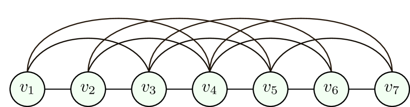
(a) a

(b) b

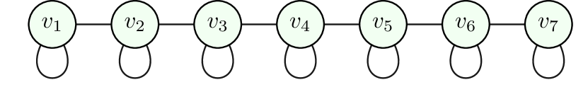
(c) c

Figure 1: Illustration of the $M$-EPG graph (a) and its unfolded versions: (b) Graph Unfolding 1 corresponding to $\beta=2$, and (c) Graph Unfolding 2 corresponding to $\beta=0$

V Graph Sampling: Formulation

We first develop methodologies to “unfold” an $M$-EPG to a sparser $1$-EPG for more efficient sampling in Section V-A. We formulate a sampling objective for a $1$-EPG in Section V-B. Finally, we develop sampling algorithms for $1$-EPGs without and with self-loops in Section VI-A and VI-B, respectively.

V-A Graph Unfolding

We first discuss how we unfold an original $M$-EPG ${\mathcal{G}}^{o}$, specified by a graph Laplacian matrix ${\mathbf{L}}^{o}$, to a $1$-EPG ${\mathcal{G}}$ [called simple path graph (SPG)], possibly with self-loops, specified by a tri-diagonal generalized graph Laplacian matrix ${\mathcal{L}}$. SPGs are more amenable to fast graph sampling. Specifically, we seek a Laplacian ${\mathcal{L}}$ for an SPG ${\mathcal{G}}$ such that

$${\mathbf{x}}^{\top}{\mathbf{L}}^{o}{\mathbf{x}}\leq{\mathbf{x}}^{\top}{\mathcal{L}}{\mathbf{x}},~{}~{}~{}\forall{\mathbf{x}}\in\mathbb{R}^{N}.$$ (7)

where ${\mathbf{x}}^{\top}{\mathbf{L}}^{o}{\mathbf{x}}$ is a GLR (1) [46] that quantifies the variation of signal ${\mathbf{x}}$ across a graph kernel specified by ${\mathbf{L}}^{o}$.

GLR has been used as a signal prior in graph signal restoration problems such as denoising, dequantization, and interpolation [46, 52, 53, 47, 54, 55]. Replacing ${\mathbf{x}}^{\top}{\mathbf{L}}^{o}{\mathbf{x}}$ with ${\mathbf{x}}^{\top}{\mathcal{L}}{\mathbf{x}}$ means that, in a minimization problem, we are minimizing an upper bound of GLR ${\mathbf{x}}^{\top}{\mathbf{L}}^{o}{\mathbf{x}}$.

(7) implies that ${\mathcal{L}}-{\mathbf{L}}^{o}\succeq 0$ is PSD. Next theorem ensures the PSDness of ${\mathcal{L}}-{\mathbf{L}}^{o}$ when converting an edge $(i,j)\in{\mathcal{E}}^{o}$ of positive weight $w^{o}_{i,j}>0$ in the original $M$-EPG ${\mathcal{G}}^{o}$ to possible edges $(i,k)$ and $(k,j)$ and self-loops at nodes $i$ and $j$ and intermediate node $k$ in the unfolded SPG ${\mathcal{G}}$.

Theorem 1.

Given a graph ${\mathcal{G}}^{o}$ specified by generalized graph Laplacian ${\mathbf{L}}^{o}$, to replace an edge $(i,j)$ of weight $w^{o}_{i,j}>0$ connecting nodes $i$ and $j$ in ${\mathcal{G}}^{o}$, a procedure that adds edges $(i,k)$ and $(k,j)$ to/from intermediate node $k$ in graph ${\mathcal{G}}$, each of weight $\beta w^{o}_{i,j}$, adds self-loops at nodes $i$ and $j$, each of weight $(2-\beta)w^{o}_{i,j}$, and adds self-loop at node $k$ of weight $(\beta^{2}-2\beta)w^{o}_{i,j}$, for $\beta\in\mathbb{R}$, results in generalized graph Laplacian ${\mathcal{L}}$ for modified graph ${\mathcal{G}}$ such that ${\mathcal{L}}-{\mathbf{L}}^{o}$ is PSD.

See Fig. 2 for an illustration of an edge $(i,j)$ in original graph ${\mathcal{G}}^{o}$ replaced by edges $(i,j-1)$ and $(j-1,j)$ and self-loops at nodes $i$, $j-1$ and $j$, each with different weights.

Proof.

GLR ${\mathbf{x}}^{\top}{\mathcal{L}}{\mathbf{x}}$ for generalized Laplacian ${\mathcal{L}}$ of graph ${\mathcal{G}}$ with edge weights $w_{i,j}$’s and self-loop weights $u_{i}$’s, can be written as a weighted sum of connected sample pair difference squares $(x_{i}-x_{j})^{2}$ and sample energies $x_{i}^{2}$ (1):

$${\mathbf{x}}^{\top}{\mathcal{L}}{\mathbf{x}}=\sum_{(i,j)\in{\mathcal{E}}}w_{i,j}(x_{i}-x_{j})^{2}+\sum_{i\in{\mathcal{V}}}u_{i}x_{i}^{2}.$$ (8)

Considering only edge $(i,j)\in{\mathcal{E}}^{o}$ in graph ${\mathcal{G}}^{o}$, its contribution to GLR ${\mathbf{x}}^{\top}{\mathbf{L}}^{o}{\mathbf{x}}$ is

$$w^{o}_{i,j}(x_{i}-x_{j})^{2}=w^{o}_{i,j}(x_{i}^{2}-2x_{i}x_{j}+x_{j}^{2}).$$ (9)

Algebraically, starting from $0\leq y^{2},~{}\forall y\in\mathbb{R}$, we write

$$0\leq(a-\beta b+c)^{2} =a^{2}-2\beta ab+2ac+\beta^{2}b^{2}-2\beta bc+c^{2}$$

$$-2ac \leq\beta(a-b)^{2}+\beta(b-c)^{2}$$

$$~{}~{}+(1-\beta)a^{2}+(\beta^{2}-2\beta)b^{2}+(1-\beta)c^{2}.$$

Letting $a=x_{i}$, $c=x_{j}$ and $b=x_{k}$ for some intermediate node $k$, we can now upper-bound $(x_{i}-x_{j})^{2}$ as

$$x_{i}^{2}-2x_{i}x_{j}+x_{j}^{2} \leq\beta(x_{i}-x_{k})^{2}+\beta(x_{k}-x_{j})^{2}$$

$$~{}~{}+(2-\beta)x_{i}^{2}+(\beta^{2}-2\beta)x_{k}^{2}+(2-\beta)x_{j}^{2}$$

Thus, replacing edge $(i,j)$ of positive weight $w^{o}_{i,j}$ in ${\mathcal{G}}^{o}$ with edges $(i,k)$ and $(k,j)$ to/from intermediate node $k$, each with weight $\beta w^{o}_{i,j}$, and self-loops at nodes $i$, $k$ and $j$ with weights $(2-\beta)w^{o}_{i,j}$, $(\beta^{2}-2\beta)w^{o}_{i,j}$ and $(2-\beta)w^{o}_{i,j}$ in ${\mathcal{G}}$, means that ${\mathbf{x}}^{\top}{\mathbf{L}}^{o}{\mathbf{x}}\leq x^{\top}{\mathcal{L}}{\mathbf{x}},\forall{\mathbf{x}}$, or ${\mathcal{L}}-{\mathbf{L}}^{o}\succeq 0$. ∎

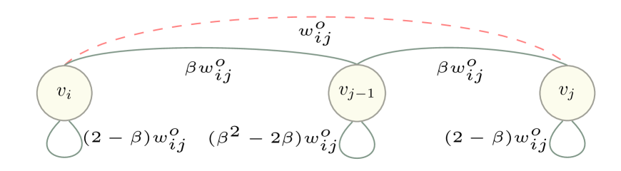
Figure 2: Graphical representation of Theorem 1: Replacing a (dashed red) edge $(i,j)$ with weight $w^{o}_{i,j}$ in the original graph ${\mathcal{G}}^{o}$ with (solid green) edges $(i,j-1)$ and $(j-1,j)$ and self-loops at nodes $i$, $j-1$ and $j$ of different weights, where $j-1$ is an intermediate node.

Given Theorem 1, we deduce two practical corollaries. The first corollary follows from Theorem 1 for $\beta=2$.

Corollary 1.

Given a graph ${\mathcal{G}}^{o}$ specified by generalized graph Laplacian ${\mathbf{L}}^{o}$, to replace an edge $(i,j)$ connecting nodes $i$ and $j$ in ${\mathcal{G}}^{o}$ of weight $w^{o}_{i,j}>0$, a procedure that adds edges $(i,k)$ and $(k,j)$ to/from intermediate node $k$ in graph ${\mathcal{G}}$, each of weight $2w^{o}_{i,j}$, results in generalized graph Laplacian ${\mathcal{L}}$ such that ${\mathcal{L}}-{\mathbf{L}}^{o}$ is PSD.

The second corollary follows from Theorem 1 for $\beta=0$.

Corollary 2.

Given a graph ${\mathcal{G}}^{o}$ specified by generalized graph Laplacian ${\mathbf{L}}^{o}$, to replace an edge $(i,j)$ connecting nodes $i$ and $j$ in ${\mathcal{G}}^{o}$ with weight $w^{o}_{i,j}>0$, a procedure that adds self-loops at nodes $i$ and $j$ in graph ${\mathcal{G}}$, each of weight $2w^{o}_{i,j}$, results in generalized graph Laplacian ${\mathcal{L}}$ for modified graph ${\mathcal{G}}$ such that ${\mathcal{L}}-{\mathbf{L}}^{o}$ is PSD.

The two corollaries represent two extreme instantiations of Theorem 1: the replacement procedure requires only adding edges/self-loops, respectively. They also lead to two graph unfolding procedures of different complexities to transform an $M$-hop EPG ${\mathcal{G}}^{o}$ to an SPG ${\mathcal{G}}$:
Graph Unfolding 1: to replace each positive edge $(i,j)$ in ${\mathcal{G}}^{o}$ with weight $w^{o}_{i,j}$ further than one hop, add edges $(i,j-1)$ and $(j-1,j)$ in ${\mathcal{G}}$ with weight $w_{i,j-1}=w_{j-1,j}=2w^{o}_{i,j}$.

Graph Unfolding 2: to replace each positive edge $(i,j)$ in ${\mathcal{G}}^{o}$ with weight $w^{o}_{i,j}$ further than one hop, add self-loops at nodes $i$ and $j$ in ${\mathcal{G}}$ with weights $u_{i}=u_{j}=2w^{o}_{i,j}$.

Specifically, in the first unfolding procedure, each unfolding of an edge $(i,j)$ in ${\mathcal{G}}^{o}$ requires $j-1$ replacement steps towards an SPG, thus a higher procedural complexity.

V-B Defining Graph Sampling Objective

Given an unfolded SPG ${\mathcal{G}}$ specified by generalized Laplacian ${\mathcal{L}}$ (see Fig. 1(b) for an illustration), we now aim to select $C$ representative sample nodes (frames) from ${\mathcal{G}}$, where $C<N$. To define a sampling objective, we first derive the worst-case reconstruction error of signal ${\mathbf{x}}\in\mathbb{R}^{N}$ given $C$ chosen samples.

Using sampling matrix ${\mathbf{H}}\in\left\{0,1\right\}^{C\times N}$ defined as

$$H_{i,j}=\left\{\begin{array}[]{ll}1&\mbox{if node $j$ is the $i$-th sample}\\ 0&\mbox{o.w.}\end{array}\right.,$$ (12)

one can choose $C$ samples from signal ${\mathbf{x}}\in\mathbb{R}^{N}$ as ${\mathbf{y}}={\mathbf{H}}{\mathbf{x}}$. To recover original signal ${\mathbf{x}}$ given observed samples ${\mathbf{y}}\in\mathbb{R}^{C}$, we employ GLR (1) as a signal prior [46], resulting in the following restoration problem:

$$\min_{{\mathbf{x}}}\|{\mathbf{y}}-{\mathbf{H}}{\mathbf{x}}\|^{2}_{2}+\mu\,{\mathbf{x}}^{\top}{\mathcal{L}}{\mathbf{x}}$$ (13)

where $\mu>0$ is a weight parameter that balances between the data fidelity and prior terms. Given (13) is quadratic, convex, and differentiable, its solution ${\mathbf{x}}^{*}$ can be obtained by solving a system of linear equations:

$$({\mathbf{H}}^{\top}{\mathbf{H}}+\mu{\mathcal{L}}){\mathbf{x}}^{*}={\mathbf{H}}^{\top}{\mathbf{y}}.$$ (14)

The coefficient matrix ${\mathbf{B}}\triangleq{\mathbf{H}}^{\top}{\mathbf{H}}+\mu{\mathcal{L}}$ is provably positive definite (PD) and thus invertible, given ${\mathcal{L}}$ is a generalized graph Laplacian for a positive connected graph.

Lemma 1.

Coefficient matrix ${\mathbf{B}}={\mathbf{H}}^{\top}{\mathbf{H}}+\mu{\mathcal{L}}$, where ${\mathbf{H}}\in\{0,1\}^{C\times N}$ is a sampling matrix, ${\mathcal{L}}$ is a positive connected graph possibly with self-loops, and $\mu>0$, is PD for $C\geq 1$.

Proof.

Note first that both ${\mathbf{H}}^{\top}{\mathbf{H}}$ and ${\mathcal{L}}$ are PSD (generalized Laplacian ${\mathcal{L}}$ for a positive graph ${\mathcal{G}}$, with or without self-loops, is provably PSD via GCT [8]). Thus, ${\mathbf{H}}^{\top}{\mathbf{H}}+\mu{\mathcal{L}}$ is PD iff there does not exist a vector ${\mathbf{v}}$ such that ${\mathbf{v}}^{\top}{\mathbf{H}}^{\top}{\mathbf{H}}{\mathbf{v}}$ and ${\mathbf{v}}^{\top}{\mathcal{L}}{\mathbf{v}}$ are simultaneously $0$. By Lemma 1 in [11], the lone first eigenvector ${\mathbf{v}}_{1}$ corresponding to the smallest eigenvalue $\lambda_{1}\geq 0$ of a generalized Laplacian ${\mathcal{L}}$ for a positive connected graph ${\mathcal{G}}$ is strictly positive (proven via the Perron-Frobenius Theorem), i.e., $v_{1,i}>0,\forall i$. Thus, ${\mathbf{v}}_{1}^{\top}{\mathbf{H}}^{\top}{\mathbf{H}}{\mathbf{v}}_{1}=\sum_{i\in{\mathcal{S}}}v_{1,i}^{2}>0$, where ${\mathcal{S}}$ is the non-empty index set for the chosen $C\geq 1$ sample nodes. So while ${\mathbf{v}}_{1}^{\top}{\mathcal{L}}{\mathbf{v}}_{1}=0$ if $\lambda_{1}=0$, ${\mathbf{v}}_{1}^{\top}{\mathbf{H}}^{\top}{\mathbf{H}}{\mathbf{v}}_{1}>0$, and hence there are no vectors ${\mathbf{v}}$ such that ${\mathbf{v}}^{\top}{\mathbf{H}}^{\top}{\mathbf{H}}{\mathbf{v}}={\mathbf{v}}^{\top}{\mathcal{L}}{\mathbf{v}}=0$. Therefore, ${\mathbf{B}}={\mathbf{H}}^{\top}{\mathbf{H}}+\mu{\mathcal{L}}$ is PD for $\mu>0$. ∎

Note that ${\mathbf{H}}^{\top}{\mathbf{H}}$ is an $N\times N$ diagonal matrix, whose diagonal entries corresponding to $C$ selected nodes are $1$, and $0$ otherwise. For convenience, we define ${\mathbf{h}}\triangleq\{0,1\}^{N}$ as a 0-1 vector of length $N$, and ${\mathbf{H}}^{\top}{\mathbf{H}}=\text{diag}\mspace{-3.0mu}\left({\mathbf{h}}\right)$.

One can show that maximizing the smallest eigenvalue $\lambda_{\min}({\mathbf{B}})$ of coefficient matrix ${\mathbf{B}}$—known as the E-optimality criterion in system design [56]—is equivalent to minimizing a worst-case reconstruction error (Proposition 1 in [9]). Given a sampling budget $C$, our sampling objective is thus to maximize $\lambda_{\min}({\mathbf{B}})$ using ${\mathbf{h}}$, i.e.,

$$\max_{{\mathbf{h}}}~{}\lambda_{\min}(\text{diag}\mspace{-3.0mu}\left({\mathbf{h}}\right)+\mu{\mathcal{L}}),~{}~{}~{}\mbox{s.t.}~{}\|{\mathbf{h}}\|_{1}\leq C.$$ (15)

For ease of computation, instead of $\lambda_{\min}({\mathbf{B}})$ we maximize instead the GCT lower bound $\lambda^{-}_{\min}({\mathbf{S}}{\mathbf{B}}{\mathbf{S}}^{-1})$ of the similarity transform ${\mathbf{S}}{\mathbf{B}}{\mathbf{S}}^{-1}$ of matrix ${\mathbf{B}}$ (with same set of eigenvalues as ${\mathbf{B}}$), where $\lambda^{-}_{\min}({\mathbf{S}}{\mathbf{B}}{\mathbf{S}}^{-1})\leq\lambda_{\min}({\mathbf{B}})$, i.e.,

$$\max_{{\mathbf{h}},{\mathbf{S}}}~{}\lambda^{-}_{\min}\left({\mathbf{S}}(\text{diag}\mspace{-3.0mu}\left({\mathbf{h}}\right)+\mu{\mathcal{L}}){\mathbf{S}}^{-1}\right),~{}~{}\mbox{s.t.}~{}\|{\mathbf{h}}\|_{1}\leq C$$ (16)

where ${\mathbf{S}}$ is an invertible matrix. In essence, (16) seeks to maximize the smallest Gershgorin disc left-end of matrix ${\mathbf{S}}{\mathbf{B}}{\mathbf{S}}^{-1}$ using ${\mathbf{h}}$ and ${\mathbf{S}}$, under a sampling budget $C$. For simplicity, we consider only positive diagonal matrices for ${\mathbf{S}}$, i.e., ${\mathbf{S}}=\text{diag}\mspace{-3.0mu}\left({\mathbf{s}}\right)$ and $s_{i}>0,\forall i$.

Note that our objective (16) differs from [9] in two respects. First, ${\mathcal{L}}$ in (16) is a generalized graph Laplacian for a positive graph possibly with self-loops, while [9] considers narrowly a positive graph without self-loops. Second, ${\mathcal{L}}$ corresponds to an SPG ${\mathcal{G}}$ and thus is tri-diagonal, while the combinatorial Laplacian in [9] correspond to a more general graph with unstructured node-to-node connectivity.

VI GRAPH Sampling: algorithm

We describe a linear-time algorithm for the formulated graph sampling problem (16), focusing first on the case of a SPG without self-loops in Section VI-A. We then extend the algorithm to the case of a SPG with self-loops in Section VI-B. We study fast sampling exclusively for SPGs, because an $M$-EPG modeling a video can be unfolded into a SPG with or without self-loops via the two graph unfolding procedures discussed in Section V-A.

VI-A Sampling for Simple Path Graph without Self-loops

To design an intuitive algorithm, we first swap the roles of the objective and constraint in (16) and solve instead its corresponding dual problem given threshold $0<T<1$ [9]:

$$\min_{{\mathbf{h}},{\mathbf{S}}}\|{\mathbf{h}}\|_{1}~{}~{}\mbox{s.t.}~{}~{}\lambda^{-}_{\min}\left({\mathbf{S}}(\text{diag}\mspace{-3.0mu}\left({\mathbf{h}}\right)+\mu{\mathcal{L}}){\mathbf{S}}^{-1}\right)\geq T.$$ (17)

In words, (17) minimizes the number of samples needed to move all Gershgorin disc left-ends of similarity-transformed matrix ${\mathbf{S}}{\mathbf{B}}{\mathbf{S}}^{-1}$ to at least $T$. It was shown in [9] that $T$ is inversely proportional to objective $\|{\mathbf{h}}^{*}\|_{1}$ of the optimal solution ${\mathbf{h}}^{*}$ to (17). Thus, to find the dual optimal solution ${\mathbf{h}}^{*}$ to (17) such that $\|{\mathbf{h}}^{*}\|_{1}=C$—and hence the optimal solution ${\mathbf{h}}^{*}$ also to the primal problem (16) [9]—one can perform binary search to find an appropriate $T$. We describe a fast algorithm to approximately solve (17) for a given $T$ next.

We first state a lemma that allows us to optimize (17) for a reduced graph ${\mathcal{G}}^{\prime}$ containing the same node set ${\mathcal{V}}$ as the original positive graph ${\mathcal{G}}$, and a reduced edge subset ${\mathcal{E}}^{\prime}\subset{\mathcal{E}}$.

Lemma 2.

Denote by ${\mathcal{G}}^{\prime}({\mathcal{V}},{\mathcal{E}}^{\prime},{\mathbf{W}}^{\prime})$ a reduced graph from positive graph ${\mathcal{G}}({\mathcal{V}},{\mathcal{E}},{\mathbf{W}})$, where edges $(i,j)\in{\mathcal{E}}\setminus{\mathcal{E}}^{\prime}$ were selectively removed. Denote by ${\mathcal{L}}^{\prime}$ and ${\mathcal{L}}$ the generalized Laplacians for graphs ${\mathcal{G}}^{\prime}$ and ${\mathcal{G}}$, respectively. Then,

$$\lambda_{\min}\left(\text{diag}\mspace{-3.0mu}\left({\mathbf{h}}\right)+\mu{\mathcal{L}}^{\prime})\leq\lambda_{\min}(\text{diag}\mspace{-3.0mu}\left({\mathbf{h}}\right)+\mu{\mathcal{L}}\right).$$ (18)

Proof.

Since ${\mathbf{x}}^{\top}{\mathcal{L}}{\mathbf{x}}$ is a weighted sum of sample difference squares and sample energies (1), for any ${\mathbf{x}}\in\mathbb{R}^{N}$,

$${\mathbf{x}}^{\top}({\mathcal{L}}-{\mathcal{L}}^{\prime}){\mathbf{x}}=\sum_{(i,j)\in{\mathcal{E}}\setminus{\mathcal{E}}^{\prime}}w_{i,j}(x_{i}-x_{j})^{2}\stackrel{{\scriptstyle(a)}}{{\geq}}0$$ (19)

where $(a)$ is true since $w_{i,j}\geq 0$ for positive graph ${\mathcal{G}}$. Thus,

$${\mathbf{x}}^{\top}(\text{diag}\mspace{-3.0mu}\left({\mathbf{h}}\right)+\mu{\mathcal{L}}^{\prime}){\mathbf{x}}\leq{\mathbf{x}}^{\top}(\text{diag}\mspace{-3.0mu}\left({\mathbf{h}}\right)+\mu{\mathcal{L}}){\mathbf{x}},~{}~{}~{}\forall{\mathbf{x}}.$$ (20)

Since this inequality includes the first (unit-norm) eigenvector ${\mathbf{v}}_{1}$ of $\text{diag}\mspace{-3.0mu}\left({\mathbf{h}}\right)+\mu{\mathcal{L}}$ corresponding to the smallest eigenvalue,

$${\mathbf{v}}_{1}^{\top}(\text{diag}\mspace{-3.0mu}\left({\mathbf{h}}\right)+\mu{\mathcal{L}}^{\prime}){\mathbf{v}}_{1}\leq\lambda_{\min}(\text{diag}\mspace{-3.0mu}\left({\mathbf{h}}\right)+\mu{\mathcal{L}}).$$ (21)

Since the left side is at least $\lambda_{\min}(\text{diag}({\mathbf{h}})+\mu{\mathcal{L}}^{\prime})$, the lemma is proven. ∎

Lemma 2 applies to any reduced graph ${\mathcal{G}}^{\prime}$ with removed edges $(i,j)\in{\mathcal{E}}\setminus{\mathcal{E}}^{\prime}$. Particularly useful in our algorithm development is when ${\mathcal{G}}^{\prime}$ is a disconnected graph ${\mathcal{G}}^{\prime}({\mathcal{V}}_{1}^{\prime}\cup{\mathcal{V}}_{2}^{\prime},{\mathcal{E}}_{1}^{\prime}\cup{\mathcal{E}}_{2}^{\prime},{\mathbf{W}}^{\prime})$ for ${\mathcal{V}}_{1}^{\prime}\cap{\mathcal{V}}_{2}^{\prime}=\emptyset$ and ${\mathcal{V}}_{1}^{\prime}\cup{\mathcal{V}}_{2}^{\prime}={\mathcal{V}}^{\prime}$, where edge set ${\mathcal{E}}^{\prime}_{1}$ (${\mathcal{E}}^{\prime}_{2}$) connects only nodes in ${\mathcal{V}}^{\prime}_{1}$ (${\mathcal{V}}^{\prime}_{2}$). In other words, edges $(i,j)$ where $i\in{\mathcal{E}}^{\prime}_{1}$ and $j\in{\mathcal{E}}^{\prime}_{2}$ are all removed in ${\mathcal{G}}^{\prime}$. With appropriate node reordering, the adjacency matrix for ${\mathcal{G}}^{\prime}$ is block-diagonal, i.e., ${\mathbf{W}}^{\prime}=\text{diag}\mspace{-3.0mu}\left({\mathbf{W}}^{\prime}_{1},{\mathbf{W}}^{\prime}_{2}\right)$, where ${\mathbf{W}}^{\prime}_{1}$ and ${\mathbf{W}}^{\prime}_{2}$ are the adjacency matrices for the two sub-graphs disconnected from each other. We state a useful corollary.

Corollary 3.

Suppose ${\mathcal{G}}^{\prime}({\mathcal{V}}_{1}^{\prime}\cup{\mathcal{V}}_{2}^{\prime},{\mathcal{E}}_{1}^{\prime}\cup{\mathcal{E}}_{2}^{\prime},{\mathbf{W}}^{\prime})$ is a reduced disconnected graph from original graph ${\mathcal{G}}({\mathcal{V}},{\mathcal{E}},{\mathbf{W}})$, where ${\mathbf{W}}^{\prime}=\text{diag}\mspace{-3.0mu}\left({\mathbf{W}}^{\prime}_{1},{\mathbf{W}}^{\prime}_{2}\right)$. Then,

$$\min_{i\in\{1,2\}}\lambda_{\min}(\text{diag}\mspace{-3.0mu}\left({\mathbf{h}}_{i}\right)+\mu{\mathcal{L}}_{i}^{\prime})\leq\lambda_{\min}(\text{diag}\mspace{-3.0mu}\left({\mathbf{h}}\right)+\mu{\mathcal{L}}),$$ (22)

where ${\mathbf{h}}_{i}$ is the sub-vector of ${\mathbf{h}}$ corresponding to nodes ${\mathcal{V}}_{i}^{\prime}$, ${\mathcal{L}}_{i}^{\prime}$ is the generalized Laplacian for sub-graph $i$, and ${\mathcal{L}}$ is the generalized Laplacian for graph ${\mathcal{G}}$.

Proof.

By Lemma 2, we know that for Laplacian ${\mathcal{L}}^{\prime}$ of reduced disconnected graph ${\mathcal{G}}^{\prime}$,

$$\lambda_{\min}(\text{diag}\mspace{-3.0mu}\left({\mathbf{h}}\right)+\mu{\mathcal{L}}^{\prime})\leq\lambda_{\min}(\text{diag}\mspace{-3.0mu}\left({\mathbf{h}}\right)+\mu{\mathcal{L}}).$$ (23)

From linear algebra, we also know that for a block-diagonal matrix $\text{diag}\mspace{-3.0mu}\left({\mathbf{h}}\right)+\mu{\mathcal{L}}^{\prime}$ with sub-block matrices $\text{diag}\mspace{-3.0mu}\left({\mathbf{h}}_{1}\right)+\mu{\mathcal{L}}^{\prime}_{1}$ and $\text{diag}\mspace{-3.0mu}\left({\mathbf{h}}_{2}\right)+\mu{\mathcal{L}}^{\prime}_{2}$,

$$\min_{i\in\{1,2\}}\lambda_{\min}(\text{diag}\mspace{-3.0mu}\left({\mathbf{h}}_{i}\right)+\mu{\mathcal{L}}_{i}^{\prime})=\lambda_{\min}(\text{diag}\mspace{-3.0mu}\left({\mathbf{h}}\right)+\mu{\mathcal{L}}^{\prime}).$$ (24)

Thus, the corollary is proven. ∎

Given Corollary 3, the main idea to solve (17) is divide-and-conquer: to maintain threshold $T$ of lower bound $\lambda_{\min}^{-}(\text{diag}\mspace{-3.0mu}\left({\mathbf{h}}\right)+\mu{\mathcal{L}})$, identify one sample node $k$ such that left-ends of Gershgorin discs corresponding to the first $d$ nodes can be moved beyond $T$. We then recursively solve the same sampling problem for sub-graph ${\mathcal{G}}^{\prime}$ with subset of nodes $\{d+1,\ldots N\}$.

Specifically, given generalized Laplacian ${\mathcal{L}}$ for SPG ${\mathcal{G}}$, we solve

$$\max_{k,{\mathbf{S}}^{d}}~{}d,~{}~{}\mbox{s.t.}~{}~{}\lambda^{-}_{\min}({\mathbf{S}}^{d}(\text{diag}\mspace{-3.0mu}\left({\mathbf{e}}_{k}\right)+\mu{\mathcal{L}}^{d})({\mathbf{S}}^{d})^{-1})\geq T$$ (25)

where ${\mathbf{e}}_{k}\in\{0,1\}^{d}$ is a length-$d$ canonical vector with only one non-zero entry $e_{k,k}=1$, ${\mathcal{L}}^{d}$ is the generalized Laplacian for the sub-graph containing only the first $d$ nodes, and ${\mathbf{S}}^{d}$ is a diagonal $d\times d$ matrix. In words, (25) seeks a single sample node $k$ and similarity transform matrix ${\mathbf{S}}^{d}$, so that disc left-ends of the first $d$ nodes move beyond $T$.

To solve (25) efficiently, we first assume that SPG ${\mathcal{G}}$ has no self-loops. The implication is that all Gershgorin discs $i$ of generalized Laplacian ${\mathcal{L}}$ have left-ends $c_{i}-r_{i}$ at $0$, i.e.,

$${\mathcal{L}}_{i,i}-\sum_{j\neq i}|{\mathcal{L}}_{i,j}|=\sum_{j\neq i}W_{i,j}-\sum_{j\neq i}W_{i,j}=0,~{}~{}\forall i.$$ (26)

This means that a sample node $k$ and transform matrix ${\mathbf{S}}^{d}$ must move all disc left-ends from $0$ to $T$.

VI-A1 Downstream Coverage Computation

Before we describe our upstream sampling algorithm, we first review a downstream procedure in [9] that progressively identifies a set of neighboring nodes $j$ to $k$ with Gershgorin disc left-ends that can move beyond $T$, given node $k$ is chosen as a sample. We say sample node $k$ “covers” nodes $j$ in a neighborhood ${\mathcal{N}}_{k}$; the downstream procedure identifies ${\mathcal{N}}_{k}$ for sample $k$.

Sampling $k$ means $h_{k}=1$, and thus diagonal entry $B_{k,k}$—center of disc $k$ corresponding to node $k$—is increased by $1$. One can now expand the radius of disc $k$ by factor $s_{k}^{u}>1$ so that left-end of disc $k$ is at $T$ exactly, i.e.,

$${\mathcal{L}}_{k,k}+1-s_{k}(W_{k,k-1}+W_{k,k+1}) \geq T$$

$$s_{k}^{u}\triangleq\frac{{\mathcal{L}}_{k,k}+1-T}{W_{k,k-1}+W_{k,k+1}}.$$ (27)

$s_{k}^{u}$ is a “maximum” in the sense that any larger scalar $s_{k}>s_{k}^{u}$ would reduce disc $k$ left-end to smaller than $T$.

Scalar $s_{k}^{u}>1$ also means reducing the $(k+1,k)$-entry of matrix ${\mathbf{S}}{\mathbf{B}}{\mathbf{S}}^{-1}$ to $(s_{k}^{u})^{-1}W_{k+1,k}$, and thus reducing disc $k+1$ radius. For disc $k+1$ left-end to pass $T$, the following inequality must be satisfied:

$${\mathcal{L}}_{k+1,k+1}-s_{k+1}((s_{k}^{u})^{-1}W_{k+1,k}+W_{k+1,k+2}) \geq T$$

$$s_{k+1}^{u}\triangleq\frac{{\mathcal{L}}_{k+1,k+1}-T}{(s_{k}^{u})^{-1}W_{k+1,k}+W_{k+1,k+2}}.$$ (28)

If $s_{k+1}^{u}<1$, then sample $k$ cannot cover node $k+1$. Otherwise, sample $k$ covers node $k+1$, and we add $k+1$ to ${\mathcal{N}}_{k}$. Using $s_{k+1}^{u}$ we check if $s_{k+2}^{u}<1$ for coverage of node $k+2$, and so on. In essence, the benefit of sampling node $k$ is propagated downstream through a chain of connected nodes $j$ along SPG ${\mathcal{G}}$ via scalars $s_{j}^{u}>1$.

The same procedure can be done for nodes $j$ with indices $j<k$ as well to identify nodes $j$ in the coverage neighborhood ${\mathcal{N}}_{k}$ (See Fig. 3).

Figure 3: Illustration of Shifting and Scaling operations in Gershgorin Disk Alignment. (Initial): The example shows a simple path graph with $4$ nodes denoted by $v_{1},v_{2},\dots,v_{4}$, connected by edges with weights $w_{i,i+1}=0.5$, $\forall i=1,2,\dots,3$. The matrix represented here is $\mathbf{B}=\text{diag}\mspace{-3.0mu}\left(\mathbf{h}\right)+\mu\mathbf{L}$, where $\mathbf{L}$ denotes the Laplacian matrix. Initially, all disc left-ends are located at $0$. (Shift): Upon sampling node $v_{3}$, its corresponding disc, $\mathcal{D}_{3}$, is shifted right by $1$. (Scale): The application of scalar $s_{3}=1.9$ causes $\mathcal{D}_{3}$’s left-end to align at $T=0.1$, while the reciprocal scalars $1/s_{3}$ decrease the radii of $\mathcal{D}_{2}$ and $\mathcal{D}_{4}$ subsequently.

VI-A2 Upstream Sampling Algorithm

We now derive an upstream procedure to select a single sample $k$ and diagonal matrix ${\mathbf{S}}^{d}=\text{diag}\mspace{-3.0mu}\left({\mathbf{s}}_{d}\right)$ for problem (25). In essence, it is the reverse of the downstream procedure described earlier: starting from node $1$, we find the furthest sample $k$ that would cover all nodes $1,\ldots,k-1$ by computing minimal scalars $s_{i}^{l}$’s that ensure coverage of nodes $i\in\{1,\ldots,k-1\}$.

Starting from node $1$, setting $s_{1}=1$, the minimum scalar $s_{2}^{l}>1$ needed to move left-end of disc $1$ beyond $T$ is

$${\mathcal{L}}_{1,1}-s_{2}^{-1}W_{1,2} \geq T$$

$$s_{2}^{l}\triangleq\frac{W_{1,2}}{{\mathcal{L}}_{1,1}-T}.$$ (29)

$s_{2}^{l}$ is a “minimum” value in the sense that any smaller scalar $s_{2}<s_{2}^{l}$ would not move disc $1$ left-end beyond $T$.

If node $2$ is sampled, then the maximum scalar $s_{2}$ while ensuring disc $2$ left-end moves beyond $T$ is $s_{2}^{u}$. If $s^{u}_{2}<s^{l}_{2}$, then the maximum scalar $s_{2}^{u}$ by sample $2$ is not large enough to meet the minimum scalar $s_{2}^{l}$ required by node $1$. Hence, sampling node $2$ cannot cover node $1$, and node $1$ must be sampled. In this case, sample node is $k=1$, and maximal $d$ can be determined by identifying coverage ${\mathcal{N}}_{1}$ via the aforementioned downstream procedure.

If $s^{u}_{2}\geq s^{l}_{2}$, then sampling node $2$ can cover node $1$, and hence $k>1$. But does node $2$ need to be sampled?

If node $2$ is also not sampled, then using $s_{2}^{l}$ (to ensure node $1$ is covered), the minimum scalar $s_{3}^{l}\geq 1$ required to move disc $2$ left-end beyond $T$ is

$${\mathcal{L}}_{2,2}-s_{2}^{l}(W_{2,1}+s_{3}^{-1}W_{2,3}) \geq T$$

$$s_{3}^{l}\triangleq\frac{s_{2}^{l}W_{2,3}}{{\mathcal{L}}_{2,2}-s^{l}_{2}W_{2,1}-T}.$$ (30)

If node $3$ is a sampled node, then the maximum scalar $s_{3}^{u}$ while moving disc $3$ left-end beyond $T$ is

$${\mathcal{L}}_{3,3}+1-s_{3}((s_{2}^{l})^{-1}W_{3,2}+W_{3,4}) \geq T$$

$$s_{3}^{u}\triangleq\frac{{\mathcal{L}}_{3,3}+1-T}{(s_{2}^{l})^{-1}W_{3,2}+W_{3,4}}.$$ (31)

If $s_{3}^{u}<s_{3}^{l}$, then the maximum scalar $s_{3}^{u}$ by sample $3$ is not large enough to satisfy the minimum scalar $s_{3}^{l}$ required by node $2$. Thus, node $2$ must be sampled. On the other hand, if $s_{3}^{u}\geq s_{3}^{l}$, then sampling node $3$ can cover nodes $2$ and $1$.

We can now generalize the previous analysis to an algorithm to determine a single sample node $k$ as follows.

1. Initialize $s_{1}^{l}=1$, $W_{1,0}=0$, and $i=1$.

2. Compute minimum scalar $s_{i+1}^{l}$ required to cover downstream nodes $i,\ldots,1$:

   $$s_{i+1}^{l}\triangleq\frac{s_{i}^{l}W_{i,i+1}}{{\mathcal{L}}_{i,i}-s_{i}^{l}W_{i,i-1}-T}.$$ (32)

3. Compute maximum scalar $s_{i+1}^{u}$ if node $i+1$ is sampled.

   $$s_{i+1}^{u}\triangleq\frac{{\mathcal{L}}_{i+1,i+1}+1-T}{(s_{i}^{l})^{-1}W_{i+1,i}+W_{i+1,i+2}}.$$ (33)

   If $s_{i+1}^{u}<s_{i+1}^{l}$ or $s_{i+1}^{l}<1$, then $k\leftarrow i$ and $s_{k}^{l}\leftarrow s_{k}^{u}$. Exit.

4. Given $s_{i+1}^{u}\geq s_{i+1}^{l}$ and $s_{i+1}^{l}\geq 1$, increment $i$ and goto step 2.

Given sample $k$, one can compute $d$ via procedure in Section VI-A1. The summary of the algorithm discussed here is depicted in Algorithm 1.

Algorithm 1 Greedy Elaborate Path Graph Sampling ($\beta=2$)

Input:  ${\mathcal{G}}$, $T$, $K$, $\mu$
    Output:  ${\mathcal{S}}$, Flag

  Initialize   $\Omega\leftarrow{\mathcal{V}}$, ${\mathcal{S}}\leftarrow\emptyset$, $q\leftarrow 1$

  Initialize   ${\mathbf{W}}^{q}\leftarrow{\mathbf{W}}$, Flag $\leftarrow$ False

  while $\Omega\neq\emptyset$ and $q\leq K$ do

     ${\mathcal{S}}_{k}\leftarrow$ Take the procedure’s steps 1-4 using (32), (33) to select sample node $k$.

     $\Omega_{k}\leftarrow$ Given ${\mathcal{S}}_{k}$, compute $d$ via procedure in VI-A1.

     ${\mathcal{S}}\leftarrow{\mathcal{S}}\cup{\mathcal{S}}_{k}$, $\Omega\leftarrow\Omega\setminus\Omega_{k}$

     Update ${\mathcal{G}}$ by remaining nodes in $\Omega$.

     $k\leftarrow k+1$

  end while

  if $\Omega=\emptyset$ then

     Flag $\leftarrow$ True

  end if

The next lemma states that the scalars computed during upstream sampling can indeed compose a diagonal matrix ${\mathbf{S}}^{d}$ so that the Gershgorin disc left-end condition $\lambda_{\min}^{-}({\mathbf{S}}^{d}(\text{diag}\mspace{-3.0mu}\left({\mathbf{e}}_{k}\right)+\mu{\mathcal{L}}^{d})({\mathbf{S}}^{d})^{-1})\geq T$ in problem (25) is indeed satisfied.

Lemma 3.

Using $s_{i+1}^{l}$ computed using (32) for non-sample nodes $i+1$ and $s_{i+1}^{u}$ computed using (33) for sample node $k$ to compose ${\mathbf{S}}^{d}$, $\lambda^{-}_{\min}({\mathbf{S}}^{d}(\text{diag}\mspace{-3.0mu}\left({\mathbf{e}}_{k}\right)+\mu{\mathcal{L}}^{d})({\mathbf{S}}^{d})^{-1})\geq T$.

The proof of Lemma 3 is provided in Appendix A.

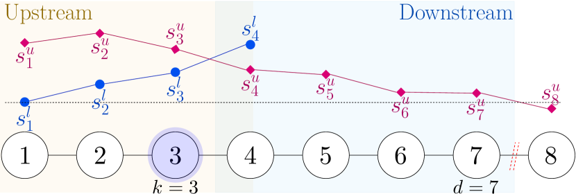
Figure 4: Illustration of upstream and Downstream procedures in an SPG graph. The algorithm iteratively computes the scalars $s^{u}_{i}$ and $s^{l}_{i}$ until $s^{u}_{i}<s^{l}_{i}$, identifying the sampled node ($k=3$). Subsequently, the downstream procedure computes the coverage of sampled node $k$ onwards. Covered nodes are then removed from the graph, allowing the sampling algorithm to proceed with the remaining SPG.

VI-B Sampling for Simple Path Graph with Self-loops

In the case of $\beta=0$ in the graph unfolding procedure (see Fig. 1c), edge sparsification introduces self-loops in the resulting SPG ${\mathcal{G}}$. Self-loops in a graph complicate our developed upstream sampling algorithm by varying the initial Gershgorin disc left-ends of Laplacian matrix ${\mathcal{L}}$.

Thanks to a recent theorem called Gershgorin Disc Perfect Alignment (GDPA) [11], we can resolve this problem by first aligning Gershgorin disc left-ends at minimum eigenvalue $\lambda_{\min}({\mathcal{L}})$ before executing our upstream sampling algorithm. Specifically, GDPA states that a similarity-transformed matrix ${\mathcal{L}}^{\prime}={\mathbf{P}}{\mathcal{L}}{\mathbf{P}}^{-1}$, where ${\mathbf{P}}=\text{diag}\mspace{-3.0mu}\left(1/v_{1,1},\ldots,1/v_{1,N}\right)$ and ${\mathbf{v}}_{1}$ is ${\mathcal{L}}$’s first strictly positive eigenvector, has Gershgorin disc left-ends perfectly aligned at $\lambda_{\min}({\mathcal{L}})$. Computing the first eigenvector ${\mathbf{v}}_{1}$ for our sparse and symmetric Laplacian matrix ${\mathcal{L}}$ can be done in linear time using Locally Optimal Block Preconditioned Conjugate Gradient (LOBPCG) [57].

Although the first eigenvector ${\mathbf{v}}_{1}$ of a generalized Laplacian ${\mathcal{L}}$ for a positive graph is provably strictly positive [11], in practice, the computation of ${\mathbf{v}}_{1}$ can be unstable when $v_{1,i}\approx 0,\exists i$. This makes the perfect alignment of disc left-ends at $\lambda_{\min}({\mathcal{L}})$ difficult. We circumvent the need to compute ${\mathbf{v}}_{1}$ directly as follows. We know that disc left-ends of similarity-transformed matrix ${\mathbf{P}}{\mathcal{L}}{\mathbf{P}}^{-1}$ are aligned at $\lambda_{\mathrm{min}}({\mathcal{L}})$, i.e.,

$$\left({\mathbf{P}}{\mathcal{L}}{\mathbf{P}}^{-1}\right)\bm{1}=\lambda_{\mathrm{min}}\bm{1}.$$ (34)

Given that ${\mathcal{L}}$ is tri-diagonal for a SPG ${\mathcal{G}}$, we can write for rows $1$ to $N-1$ of ${\mathbf{P}}{\mathcal{L}}{\mathbf{P}}^{-1}$:

$$\lambda_{\min} ={\mathcal{L}}_{1,1}-\frac{p_{1}}{p_{2}}|{\mathcal{L}}_{1,2}|$$ (35)

$$\lambda_{\min} ={\mathcal{L}}_{i,i}-\frac{p_{i}}{p_{i-1}}|{\mathcal{L}}_{i,i-1}|-\frac{p_{i}}{p_{i+1}}|{\mathcal{L}}_{i,i+1}|,~{}~{}i\in\{2,\ldots,N-1\}$$

If we now define $\alpha_{i}\triangleq\frac{p_{i}}{p_{i+1}}=\frac{v_{1,i+1}}{v_{1,i}}$, then (35) simplifies to

$$\lambda_{\min} ={\mathcal{L}}_{1,1}-\alpha_{1}|{\mathcal{L}}_{1,2}|$$ (36)

$$\lambda_{\min} ={\mathcal{L}}_{i,i}-\alpha_{i-1}^{-1}|{\mathcal{L}}_{i,i-1}|-\alpha_{i}|{\mathcal{L}}_{i,i+1}|,~{}~{}i\in\{2,\ldots,N-1\}$$

Using (36), $\alpha_{i}$ can be computed iteratively from $i=1$ onwards. After disc left-ends of ${\mathbf{P}}{\mathcal{L}}{\mathbf{P}}^{-1}$ are aligned at $\lambda_{\min}({\mathcal{L}})$, our developed upstream sampling algorithm can be deployed.

VI-C Computational Complexity Analysis

To select one sample $k$, graph sampling involves a single partition. In the upstream procedure, scalars $s^{l}_{i}$ and $s^{u}_{i}$ are computed once for each node, from $i=1$ to $i=k$. This incurs a cost of ${\mathcal{O}}(\left|{\mathcal{N}}_{k}^{u}\right|)$, where ${\mathcal{N}}_{k}^{u}=\{1,2,\ldots,k\}$ represents the upstream coverage of node $k$.

The downstream procedure similarly incurs a cost of ${\mathcal{O}}(\left|{\mathcal{N}}_{k}^{d}\right|)$, where ${\mathcal{N}}_{k}^{d}=\{k+1,\ldots,d\}$ represents the coverage of node $k$ with indices larger than $k$. Combining both procedures, the total cost for each graph partition is ${\mathcal{O}}(\left|{\mathcal{N}}_{k}\right|)$, with ${\mathcal{N}}_{k}={\mathcal{N}}_{k}^{u}\cup{\mathcal{N}}_{k}^{d}$ and mutually exclusive sets ${\mathcal{N}}_{k}^{u}$ and ${\mathcal{N}}_{k}^{d}$. In general, graph sampling has a complexity of ${\mathcal{O}}(\sum_{k=1}^{K}\left|{\mathcal{N}}_{k}\right|)$, where $K$ is the number of selected nodes. Since there is no overlap in the partitioned sets, $\sum_{k=1}^{K}\left|{\mathcal{N}}_{k}\right|=N$.

Binary search with precision $\epsilon$ (e.g., $\epsilon=10^{-6}$) is used to determine the appropriate $T$ in each iteration, resulting in a total algorithm cost of ${\mathcal{O}}(N\log\frac{1}{\epsilon})$. Since $\epsilon$ is fixed and not a function of $N$, the overall computational cost is ${\mathcal{O}}(N)$.

In the case of SPG with self-loops, the computation complexity of $\lambda_{\min}({\mathcal{L}})$ using LOBPCG algorithm for sparse and symmetric graph Laplacian matrix ${\mathcal{L}}$ is linear. The iterative alignment of left-end of discs also takes ${\mathcal{O}}(N)$, and hence the overall complexity of the algorithm is ${\mathcal{O}}(N\log\frac{1}{\epsilon})$, same as the case for SPG without self-loops.

VII Experiments

We first compare the signal reconstruction quality of our graph unfolding procedure and sampling algorithm with several existing graph sampling methods. To assess the performance of video summarization, we employ several datasets, including VSUMM/OVPs and YouTube [31]. Notably, given our focus on keyframe selection for transitory videos, we created a new dataset (see Section VII-B3) to address the current problem of lacking keyframe-based video datasets on a larger scale and with flexible licensing. Finally, we present an ablation study on algorithm components.

VII-A Graph Sampling Performance

We show the efficacy of our graph unfolding procedure and sampling method specialized for $M$-EPG graphs. We conducted a signal-reconstruction experiment similar to [9], using graphs generated from videos in the VSUMM [31] dataset. The graph construction process, detailed in Section IV, generated 25 $2$-EPG graphs at $2$ frames per second (fps), resulting in graph sizes between $N=116$ and $N=230$. For edge weight computation (see (6)), we used $\sigma=6$.

To simulate graph signals for evaluation, we considered two classes of random signals, as done in [9]:

• BL Signal: The ground-truth was a bandlimited (BL) signal defined by the first $\lfloor N/20\rfloor$ eigenvectors of Laplacian ${\mathbf{L}}$, resulting in a strictly low-pass signal. The GFT coefficients are drawn from a $\mathcal{N}(1,0.5^{2})$ distribution [19].

• Gaussian Markov Random Field (GMRF): We employed a shifted version of Laplacian ${\mathbf{L}}$ as the inverse covariance (precision) matrix, i.e., a multivariate Gaussian distribution $\mathcal{N}\left(\mathbf{0},({\mathbf{L}}+\delta{\mathbf{I}})^{-1}\right)$, where $\delta=10^{-4}$, same as [9]. To ensure consistency of graph signal power, we normalized the signal power using $({\mathbf{x}}-\bar{{\mathbf{x}}})/\text{std}({\mathbf{x}})$, where $\bar{{\mathbf{x}}}$ and $\text{std}({\mathbf{x}})$ denote the mean and standard deviation of the graph signal, respectively.

To compute the reconstructed signal, we solved linear system (13) to reconstruct the signal from (noisy) observations and measured the mean squared error (MSE) for both $\lfloor N/20\rfloor$-BL and GMRF graph signals (see Fig. 5).

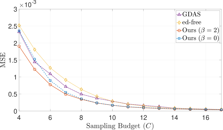
(a)

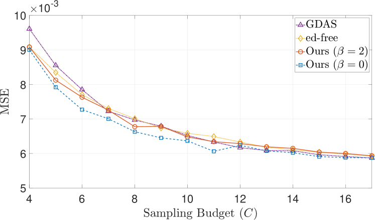
(b)

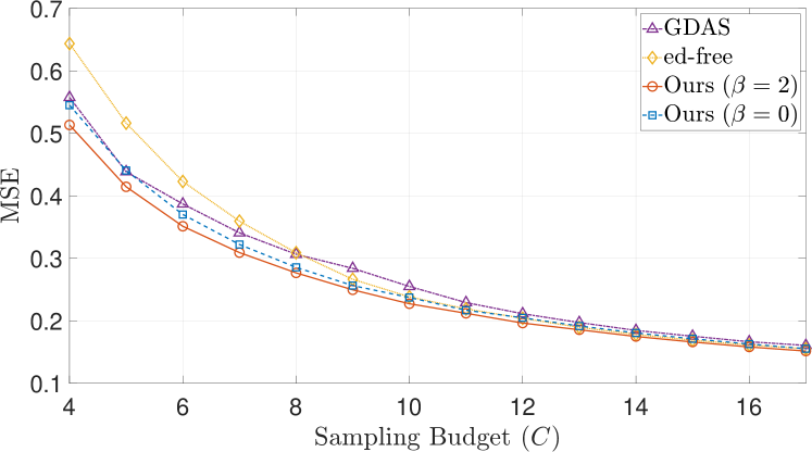
(c)

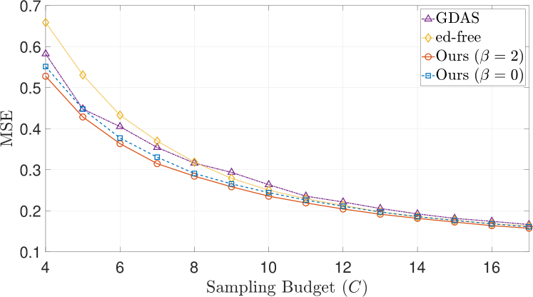
(d)

Figure 5: MSE reconstruction performance of our graph sampling algorithm for different graph signals defined on $2$-EPG graphs using GLR-based signal reconstruction in comparison to GDAS [9] and Ed-free [22]. (5a)-(5b) show results for $\lfloor\frac{N}{20}\rfloor$-BL graph signals with two different noise levels: noise-free and $20$dB, respectively. (5c)-(5d) show results for GMRF graph signals with two different noise levels: noise-free, and $20$dB, respectively.

We conducted a Monte Carlo experiment on the 25 video graphs, repeating each simulation 100 times. We tested two noise settings: noise-free signals (Fig. 5a and 5c), and $20$dB noisy signals (Fig. 5b and 5c).

As competing schemes, we used [9] and [22] on $M$-EPG graphs. For our scheme, we first unfolded each EPG graph using one of two unfolding procedures ($\beta=2$ and $\beta=0$). We then applied the two variants of our algorithm corresponding to unfolded graphs with and without self-loops. For all experiments, we set the numerical precision of binary search and the regularization parameter in GDAS-based variants to $\epsilon=10^{-9}$ and $\mu=0.05$, respectively. For Ed-free [22], we used the recommended parameters in the experiments in [9], including the Chebyshev polynomial approximation parameter of 12 and the filter width parameter of $\nu=12$.

For BL signals, when the noise level was low, the $\beta=2$ variant, which unfolded the graph to an SPG without self-loops, performed best. At higher noise levels, the $\beta=0$ variant, which unfolded the graph to an SPG with self-loops, performed best. In the case of GMRF signals, the $\beta=2$ variant maintained the best performance.

Our two unfolding variants provide different bounds on the GLR term in (7). In general, the $\beta=2$ variant offers a tighter upper bound for smooth signals, leading to better performance. Notably, for perfectly smooth signals ($x_{i}=x_{j}$ for all $(i,j)\in{\mathcal{E}}$), ${\mathbf{x}}^{\top}{\mathcal{L}}{\mathbf{x}}=0$ for $\beta=2$ (thus the tightest upper bound possible), but remains nonzero for $\beta=0$ due to self-loops. Thus, the $\beta=2$ variant exhibits a slight reconstruction advantage, although both variants outperform competitors.

VII-B Keyframe Selection Performance

VII-B1 VSUMM/OVP dataset

VSUMM [31] is the most popular dataset for keyframe-based video summarization in the literature. Collected from Open Video Project (OVP) [5], it consists of 50 videos of duration $1$-$4$ minutes and resolution of $352\times 240$ in the MPEG-1 format (mainly in 30fps). The videos are in different genres: documentary, educational, lecture, historical, etc.

Fifty human subjects participated in constructing user summaries, each annotating five videos. Thus, the dataset has five sets of keyframes as ground-truth per video, and each set may contain a different number of keyframes. Here, we refer to computer-generated keyframes as automatic summary (${\mathcal{A}}$), and the human-annotated keyframes as user summary ${\mathcal{U}}_{u}$, for each user $u\in\{1,\ldots,5\}$.

For each video, the agreements between ${\mathcal{A}}$ and each of the user summaries, $\mathcal{U}_{u}$, were evaluated using Precision ($P_{u}$), Recall ($R_{u}$), and $F_{1,u}$. We define the precision, recall, and $F_{1}$ against each human subject as follows [44, 14],

$$P_{u}=\frac{|\mathcal{A}\cap\mathcal{U}_{u}|}{|\mathcal{A}|},\quad R_{u}=\frac{|\mathcal{A}\cap\mathcal{U}_{u}|}{|\mathcal{U}_{u}|},\quad F_{1,u}=\frac{2P_{u}R_{u}}{P_{u}+R_{u}}$$

where $|{\mathcal{A}}\cap{\mathcal{U}}_{u}|$ is the number of keyframes in ${\mathcal{A}}$ matching ${\mathcal{U}}_{u}$. $|{\mathcal{A}}|$ and $|{\mathcal{U}}_{u}|$ denote the number of selected keyframes in the automatic and user summaries, respectively. For each video, we measured the mean precision, recall, and $F_{1}$ across all users. The values in Table I are the averages of these measures across all videos in the dataset. Our evaluation protocol followed VSUMM [31], and for the matching frames we used both criteria of similarity score [31] and temporal distance of $2.5$ seconds between matched frames [44, 14]. Unlike [6, 44], we did not conduct exhaustive searches for optimal keyframe numbers on a per-video basis. Instead, we employed a fixed, video-invariant sampling budget, $C$, and tuned its value to maximize the $F_{1}$ score.

For comparison, we followed [31, 14] and compared our method with DT [5], VSUMM [31], STIMO [36], MSR [45], AGDS [13] and SBOMP [14]. The results for DT, STIMO and VSUMM methods are available from the official VSUMM website. Since the other algorithm implementations or their automatic summaries are not publicly available, we relied on the best results reported in [14] for comparison.

TABLE I: Results on VSUMM

Algorithm	$P$ (%)	$R$ (%)	$F_{1}$ (%)
DT [5]	35.51	26.71	29.43
STIMO [36]	34.73	40.03	35.75
VSUMM∗ [31]	47.26	42.34	43.52
MSR [45]	36.94	57.61	43.39
AGDS [13]	37.57	64.60	45.52
SBOMP [14]	39.28	62.28	46.68
SBOMPn [14]	41.23	68.47	49.70
GDAVS [15]	39.67	72.48	48.92
Ours ($M=2$, $\beta=0$, $\mu=0.04$, $\sigma=5.62$)	36.63	83.88	49.06
Ours ($M=3$, $\beta=0$, $\mu=0.04$, $\sigma=5.62$)	35.57	81.25	47.56
Ours ($M=1$, $\mu=0.03$, $\sigma=1.0$)	39.08	71.69	48.54
Ours ($M=2$, $\beta=2$, $\mu=0.03$, $\sigma=1.0$)	40.77	74.16	50.54
Ours ($M=3$, $\beta=2$, $\mu=0.03$, $\sigma=1.0$)	31.51	57.29	39.04

Table I shows the experimental results, where the numbers in underlined bold, bold, and underlined indicate the top three performances. The significantly higher precision of the VSUMM method [31] can be attributed to its preprocessing steps, which eliminate low-quality frames, and its post-processing pruning, which removes very similar selected frames–techniques not employed by other methods. SBOMP [14] is a recently proposed video summarization method with SOTA performance and relies on sub-frame representation by extracting features for each image patch collected in a matrix block. This results in a complex representation for video frames in their dictionary learning-based solution, increasing the algorithm’s complexity—${\mathcal{O}}(Cp^{4}\ell N^{3})$, where $\ell$ is the dimension of feature vector, $p$ is the number of patches per frame, and $N,C$ are the number of frames and keyframes, respectively. While $\ell$ is fixed, the number of keyframes is typically proportional to the number of frames, i.e., $C\propto N$. This effectively increases the complexity to ${\mathcal{O}}(N^{4})$. The SBOMPn version extends the representation to the temporal dimension by considering super-blocks of patches from adjacent frames, thereby increasing the complexity.

In contrast, our graph sampling complexity is ${\mathcal{O}}(N\log_{2}\frac{1}{\epsilon})$, where $\epsilon$ is the binary search precision. Our method surpassed SBOMP and its more complex variant SBOMPn, achieving comparable performance at significantly reduced complexity.

VII-B2 YouTube Dataset

YouTube [31] serves as a dataset comparable to VSUMM/OVP, specifically designed for keyframe-based video summarization. The 50 videos, all sourced from YouTube, span genres like cartoons, news, commercials, and TV shows. Their durations range from 1 to 10 minutes.

TABLE II: Results on YouTube

Algorithm	$P$ (%)	$R$ (%)	$F_{1}$ (%)	$\overline{C}$
VSUMM∗ [31]	43.11	43.56	42.38	10.3
SMRS [39]	33.84	54.92	39.62	17.3
SSDS [58]	33.45	47.10	36.98	13.0
AGDS [13]	34.00	58.08	40.65	16.0
NSMIS [59]	35.61	59.95	41.27	18.7
GCSD [6]	37.28	54.33	42.20	13.7
SBOMP [14] ($P=1$, $E=0.05$)	32.09	44.06	35.45	13.4
SBOMP [14] ($P=5$, $E=0.05$)	32.52	45.99	36.35	14.3
Ours ($M=2$, $\beta=0$, $\mu=0.25$, $\sigma=6$)	36.87	51.11	40.89	13.9
Ours ($M=2$, $\beta=2$, $\mu=0.006$, $\sigma=6$)	37.62	56.97	42.99	15.0

Unlike VSUMM [31], the YouTube dataset is less commonly used in the literature. In this experiment, we utilized the SOTA approach by [6], which has recently demonstrated promising results on the dataset. In contrast to our previous experiment, where we employed a fixed budget ratio for all videos, according to the protocol in [6], the optimal keyframe number for each video is exhaustively searched; specifically, we searched the optimal keyframe number for each video to maximize $F_{1}$, varying from 6 to 20 with a step size of 2, as done in [6]. The evaluation process mirrors that in Section VII-B1, encompassing precision, recall, and F1 measure. Further, the benchmark yields the average budget (number of keyframes) across all videos, denoted as $\overline{C}$. Consistent with [6], we set the temporal matching criterion to 2 seconds.

Table II summarizes the evaluation results, including parameter configurations. For SBOMP [14], we used the official implementation with two patching strategies: a single patch for the entire image and the $4+1$ patching strategy from the paper. Following the recommended strategy, we generated sub-frame features for each patch and performed a parameter sweep on error thresholds (E) to report the best results. Notably, [6] builds upon [44] by incorporating an adjacency matrix into dictionary selection, increasing computational complexity, similar to [14]. Our method achieved superior performance with lower complexity, even outperforming VSUMM^∗[31], which relies on preprocessing to filter out low-quality frames and post-processing to prune redundant keyframes.

VII-B3 MHSVD Dataset

Creating datasets for video analysis is challenging due to its labor-intensive and time-consuming nature [27]. Current datasets were largely focused on longer and dynamic video summarization tasks, often neglecting the distinctive traits of short-form content prevalent on online platforms [2]. To bridge this gap, we developed a new dataset, MHSVD, specifically for transitory video summarization, with a primary emphasis on short-form content.

Dataset Collection: For this study, we gathered videos from two major video-sharing platforms, Vimeo and YouTube, using their respective filtering tools that support licensing criteria. Our selection query criteria were informed by prior research on popular video categories such as Entertainment, DIY, Comedy, etc. [60, 61], aiming to mirror their content distribution. To facilitate research and ensure ease of use, we focused on videos licensed under Creative Commons and its derivatives. Additionally, we prioritized videos based on popularity, determined by view counts. Our dataset consists of videos with a duration ranging from a minimum of $45$ seconds to a maximum of $4$ minutes, with an average duration of $110$ seconds.

Annotation: We annotate a dataset of $117$ videos, more than doubling the size of both VSUMM and YouTube datasets. Annotation was conducted using the Labelbox platform, an online tool designed for data annotation. To maintain consistency in annotations, all three annotators labeled the entire dataset once. Annotators received initial training through the platform before proceeding with annotation tasks. Each annotator watched each video in its entirety and selected up to 7 keyframes per video.

TABLE III: Results on MHSVD

Algorithm	$P$ (%)	$R$ (%)	$F_{1}$ (%)	$\overline{C}$
VSUMM [31]	31.89	50.50	37.30	7.9
SMRS [39] ($\alpha=2$, $\tau=10^{-8}$)	30.18	43.66	33.59	7.7
SBOMP [14] ($p=1$, $E=0.05$)	30.11	43.53	33.06	7.6
SBOMP [14] ($p=5$, $E=0.05$)	30.75	43.78	33.80	7.7
Ours ($M=1$, $\mu=0.2$, $\sigma=4$)	39.51	58.24	44.83	7.6
Ours ($M=2$, $\beta=0$, $\mu=0.2$, $\sigma=4$)	31.79	55.01	39.29	8.5
Ours ($M=2$, $\beta=2$, $\mu=0.2$, $\sigma=4$)	40.27	58.97	45.26	7.5

Results: Table III presents the performance evaluation of various algorithms on the MHSVD dataset. Except for [14], which provides its own implementation, we implemented all other methods for comparison on our new dataset. All methods use the same CLIP-based feature set $\left\{{\mathbf{f}}_{i}\right\}_{i=1}^{N}$ (see Section IV) except for SBOMP [14] ($p=5$), where features are generated for each sub-frame patch. The evaluation protocol followed the guidelines in Section VII-B2, but we limited the keyframe range to 1 to 11 frames due to the shorter content and fewer annotations.

We report the best performance for each competing scheme after parameter tuning. For SMRS [39], $\alpha$ and $\tau$ denote the regularization and error tolerance, respectively, with the ADMM optimization iterating 2000 times. For SBOMP [14], $p$ denotes the number of patches based on their recommended strategy. In this table, VSUMM omits pre- and post-pruning for a fair comparison, unlike VSUMM^∗ in previous experiments. Table III summarizes the results and respective parameters, highlighting the top three performances in underlined bold, bold, and underline. Our method, with parameters $M=2$ and $\beta=2$, achieved an $F_{1}$ score of 45.26%, demonstrating its effectiveness in capturing keyframes in short videos.

VII-C Ablation Study

The selection of $M$-EPG structure for video representation is grounded in the observation that consecutive video frames exhibit a high degree of similarity, a characteristic central to EPG. Importantly, this sparse graph structure enables a more efficient sampling algorithm to select keyframes. Given that it is possible for (short) videos to contain information with long-term dependencies, we performed an ablation study to validate the effectiveness of our chosen combination of EPG construction and the specialized graph sampling algorithm in processing such videos. The results of different combinations of graph construction (GC) and graph sampling (GS) algorithms are presented in Table IV.

The similarity metric between respective frame embeddings was computed using our edge computation in (6) with parameter $\sigma=6$. For both our algorithm and GDAS [9], the precision parameter was set to $\epsilon=10^{-9}$. This ablation study used the VSUMM dataset and followed the evaluation protocol, including the sampling budget, as outlined in Section VII-B1. Other parameters (shown in Table IV) were optimized via a grid search for each algorithm, with the best results reported. These parameters were: $\mu$ (regularization for [9] and our sampling), $k$ (nearest neighbor parameter), $\tau$ (threshold for $\tau$-thresholding graph construction), and $\delta$ (threshold for removing smaller weights in NNK [62]).

TABLE IV: GC/GS Ablation Study ($\sigma=6$, $\epsilon=10^{-9}$)

GC	GS	Complexity	$F_{1}$(%)
$\tau$-graph ($\tau=0.01$, $\mu=0.007$)	[9]	$\mathcal{O}(N^{2}\ell)$	$42.40$
$k$-NN ($k=25$, $\mu=0.003$)	[9]	$\mathcal{O}(N^{2}k\ell)$	$42.69$
NNK [62] ($k=50$, $\delta=0.01$, $\mu=0.006$)	[9]	$\mathcal{O}(N^{2}k\ell+Nk^{3})$	$43.59$
$1$-EPG ($\mu=0.08$)	[9]	${\mathcal{O}}(N\ell+NCP\log_{2}1/\epsilon)$	$48.55$
$2$-EPG ($\mu=0.08$)	[9]	${\mathcal{O}}(N\ell+NCP\log_{2}1/\epsilon)$	$49.13$
$3$-EPG ($\mu=0.08$)	[9]	${\mathcal{O}}(N\ell+NCP\log_{2}1/\epsilon)$	$49.21$
$4$-EPG ($\mu=0.08$)	[9]	${\mathcal{O}}(N\ell+NCP\log_{2}1/\epsilon)$	$47.92$
$1$-EPG ($\mu=0.07$)	Ours	$\mathcal{O}(N\ell+N\log_{2}1/\epsilon)$	$50.35$
$2$-EPG ($\beta=2$, $\mu=0.07$)	Ours	$\mathcal{O}(N\ell+N\log_{2}1/\epsilon)$	$50.92$
$2$-EPG ($\beta=2$, $\mu=0.07$)	Ours	$\mathcal{O}(N\ell+N\log_{2}1/\epsilon)$	$44.39$
$2$-EPG ($\beta=2.42$, $\mu=0.07$)	Ours	$\mathcal{O}(N\ell+N\log_{2}1/\epsilon)$	$51.19$

Our sampling algorithm only operates on unfolded graphs; for general graphs, we employed the method described in [9]. In the first section, we present the results of GDAS [9] sampling on general graph construction methods such as $\epsilon$-thresholding, the $k$-NN method, and NNK [62]. These methods typically produce much denser graphs compared to our sparse graph construction, especially with $\tau$-thresholding. The second section shows the results of GDAS applied to our $M$-EPG graph construction scenario. Finally, the third section provides the results of our unfolding and sampling applied to the $M$-EPG graph.

The comparison in the first section highlights the effectiveness of our graph construction. Moreover, the contrast between the second and third sections shows that our new graph sampling algorithm achieved better results for video summarization.

Further, our $M$-EPG graph construction operates with ${\mathcal{O}}(MN\ell)$ complexity, and our sampling technique runs in ${\mathcal{O}}(N\log_{2}\frac{1}{\epsilon})$ time, offering improved efficiency in both time (and memory) compared to competitors. In Table IV, $N$ denotes the number of nodes, and $C$ represents the number of samples. For [9], $P$ denotes the number of nodes within $p$ hops from a candidate node (note $P=2M$ for GDAS). In the NNK and $k$-NN graph constructions, $k$ signifies the nearest neighbor parameter. For the results in the first section of the table, we omit the sampling complexity since the graph construction dominates.

VIII Conclusion

We solve the keyframe selection problem to summarize a transitory video from a unique graph sampling perspective. Specifically, we first represent an $N$-frame transitory video as an $M$-hop path graph ${\mathcal{G}}^{o}$, where $M\ll N$, and weight $w^{o}_{i,j}$ of an edge $(i,j)$ connecting two nodes (frames) within $M$ time instants is computed using feature distance between the corresponding feature vectors ${\mathbf{f}}_{i}$ and ${\mathbf{f}}_{j}$. We unfold ${\mathcal{G}}^{o}$ into a $1$-hop path graph ${\mathcal{G}}$, specified by Laplacian ${\mathcal{L}}$, via one of two analytically derived graph unfolding procedures to lower graph sampling complexity. Given graph ${\mathcal{G}}$, we devise a linear-time algorithm that selects sample nodes specified by binary vector ${\mathbf{h}}$ to maximize the lower bound of the smallest eigenvalue $\lambda_{\min}^{-}({\mathbf{B}})$ for a coefficient matrix ${\mathbf{B}}=\text{diag}\mspace{-3.0mu}\left({\mathbf{h}}\right)+\mu{\mathcal{L}}$. Experiments show that our proposed method achieved comparable performance to SOTA methods at a reduced complexity.

Appendix A Proof of lemma 3

Proof.

Define ${\mathbf{S}}^{d}=\text{diag}\mspace{-3.0mu}\left(s_{1}^{l},\ldots,s_{d}^{l}\right)$. First, consider row $k$ of matrix ${\mathbf{S}}^{d}(\text{diag}\mspace{-3.0mu}\left({\mathbf{e}}_{k}\right)+\mu{\mathcal{L}}^{d})({\mathbf{S}}^{d})^{-1}$ corresponding to sample node $k$. The disc left-end is

$${\mathcal{L}}_{k,k}+1-s_{k}^{u}\left((s_{k-1}^{l})^{-1}W_{k,k-1}+(s_{k+1}^{l})^{-1}W_{k,k+1}\right)$$

$$\stackrel{{\scriptstyle(a)}}{{\leq}} {\mathcal{L}}_{k,k}+1-s_{k}^{u}\left((s_{k-1}^{l})^{-1}W_{k,k-1}+W_{k,k+1}\right)$$

$$\stackrel{{\scriptstyle(b)}}{{=}} {\mathcal{L}}_{k,k}+1-\left({\mathcal{L}}_{i+1,i+1}+1-T\right)=T.$$ (37)

$(a)$ is true since $s_{k+1}^{l}\geq 1$, and $(b)$ is true by definition of $s_{k}^{u}$ in (33). Consider next row $i$ of matrix ${\mathbf{S}}^{d}(\text{diag}\mspace{-3.0mu}\left({\mathbf{e}}_{k}\right)+\mu{\mathcal{L}}^{d})({\mathbf{S}}^{d})^{-1}$ corresponding to a non-sample node $i\in\{2,\ldots,k-1\}$. The disc left-end is

$${\mathcal{L}}_{i,i}-s_{i}^{l}\left((s_{i-1}^{l})^{-1}W_{i,i-1}+(s_{i+1}^{l})^{-1}W_{i,i+1}\right)$$

$$\stackrel{{\scriptstyle(a)}}{{\leq}} {\mathcal{L}}_{i,i}-s_{i}^{l}\left(W_{i,i-1}+(s_{i+1}^{l})^{-1}W_{i,i+1}\right)$$

$$\stackrel{{\scriptstyle(b)}}{{=}} {\mathcal{L}}_{i,i}-s_{i}^{l}\left(W_{i,i-1}+\frac{{\mathcal{L}}_{i,i}-s_{i}^{l}W_{i,i-1}-T}{s_{i}^{l}W_{i,i+1}}W_{i,i+1}\right)$$

$$= {\mathcal{L}}_{i,i}-s_{i}^{l}W_{i,i-1}-{\mathcal{L}}_{i,i}+s_{i}^{l}W_{i,i-1}+T=0$$ (38)

$(a)$ is true since $s_{i-1}^{l}\geq 1$, and $(b)$ is true by definition of $s_{i+1}^{l}$ in (32). One can similarly show that for $i=1$, given $s_{1}=1$ and $W_{1,0}=0$, disc left-end is simply

$${\mathcal{L}}_{1,1}-(s_{2}^{l})^{-1}W_{1,2}$$

$$= {\mathcal{L}}_{1,1}-\frac{{\mathcal{L}}_{1,1}-T}{W_{1,2}}W_{1,2}=T$$ (39)

Since disc left-ends for nodes $i\in\{1,\ldots,k\}$ are all beyond $T$, the lemma is proven. ∎

References

- [1] C. Violot, T. Elmas, I. Bilogrevic, and M. Humbert, “Shorts vs. regular videos on youtube: A comparative analysis of user engagement and content creation trends,” in Proc. ACM Web Science Conf., New York, NY, USA, 2024, p. 213–223.
- [2] Y. Zhang, Y. Liu, L. Guo, and J. Y. B. Lee, “Measurement of a large-scale short-video service over mobile and wireless networks,” IEEE Trans. Mobile Comput., vol. 22, no. 6, pp. 3472–3488, 2023.
- [3] W. Hu, N. Xie, L. Li, X. Zeng, and S. Maybank, “A Survey on Visual Content-Based Video Indexing and Retrieval,” IEEE Trans. Syst., Man, Cybern. C, Appl. Rev., vol. 41, no. 6, pp. 797–819, Nov. 2011.
- [4] D. Brezeale and D. J. Cook, “Automatic Video Classification: A Survey of the Literature,” IEEE Trans. Syst. Man, Cybern. C, Appl. Rev., vol. 38, no. 3, pp. 416–430, May 2008.
- [5] P. Mundur, Y. Rao, and Y. Yesha, “Keyframe-based video summarization using Delaunay clustering,” Int. J. Digital Libraries, vol. 6, no. 2, pp. 219–232, Apr. 2006.
- [6] M. Ma, S. Mei, S. Wan, Z. Wang, X.-S. Hua, and D. D. Feng, “Graph Convolutional Dictionary Selection With L2,p Norm for Video Summarization,” IEEE Trans. Image Process., vol. 31, pp. 1789–1804, 2022.
- [7] A. Ortega, P. Frossard, J. Kovacevic, J. M. F. Moura, and P. Vandergheynst, “Graph signal processing: Overview, challenges, and applications,” Proc. IEEE, vol. 106, no.5, pp. 808–828, May 2018.
- [8] G. Cheung, E. Magli, Y. Tanaka, and M. Ng, “Graph spectral image processing,” Proc. IEEE, vol. 106, no.5, pp. 907–930, May 2018.
- [9] Y. Bai, F. Wang, G. Cheung, Y. Nakatsukasa, and W. Gao, “Fast graph sampling set selection using gershgorin disc alignment,” IEEE Trans. Signal Process., vol. 68, pp. 2419–2434, 2020.
- [10] R. S. Varga, Gergorin and His Circles. Springer, 2004.
- [11] C. Yang, G. Cheung, and W. Hu, “Signed graph metric learning via gershgorin disc perfect alignment,” IEEE Trans. Pattern Anal. Mach. Intell., vol. 44, no. 10, pp. 7219–7234, 2022.
- [12] S. Mei, G. Guan, Z. Wang, M. He, X.-S. Hua, and D. Dagan Feng, “L2,0 constrained sparse dictionary selection for video summarization,” in Proc. IEEE Int. Conf. Multimedia Expo, Jul. 2014, pp. 1–6.
- [13] Y. Cong, J. Liu, G. Sun, Q. You, Y. Li, and J. Luo, “Adaptive greedy dictionary selection for web media summarization,” IEEE Trans. Image Process., vol. 26, no. 1, pp. 185–195, Jan. 2017.
- [14] S. Mei, M. Ma, S. Wan, J. Hou, Z. Wang, and D. D. Feng, “Patch Based Video Summarization With Block Sparse Representation,” IEEE Trans. Multimedia, vol. 23, pp. 732–747, 2021.
- [15] S. Sahami, G. Cheung, and C.-W. Lin, “Fast Graph Sampling for Short Video Summarization Using Gershgorin Disc Alignment,” in Proc. IEEE Int. Conf. Acoustics, Speech, Signal Process., May 2022, pp. 1765–1769.
- [16] G. Puy, N. Tremblay, R. Gribonval, and P. Vandergheynst, “Random sampling of bandlimited signals on graphs,” Appl. Computat. Harmonic Anal.s, vol. 44, no. 2, pp. 446–475, 2018.
- [17] G. Puy and P. Pérez, “Structured sampling and fast reconstruction of smooth graph signals,” Information and Inference: A Journal of the IMA, vol. 7, no. 4, pp. 657–688, 2018.
- [18] S. Chen, R. Varma, A. Sandryhaila, and J. Kovacevic, “Discrete signal processing on graphs: Sampling theory,” IEEE Trans. Signal Process., vol. 63, no. 24, pp. 6510–6523, 2015.
- [19] A. Anis, A. Gadde, and A. Ortega, “Efficient sampling set selection for bandlimited graph signals using graph spectral proxies,” IEEE Trans. Signal Process., vol. 64, no. 14, pp. 3775–3789, 2016.
- [20] F. Wang, Y. Wang, and G. Cheung, “A-optimal sampling and robust reconstruction for graph signals via truncated Neumann series,” in IEEE Signal Process. Lett., vol. 25, no.5, May 2018, pp. 680–684.
- [21] A. Ortega, Introduction to graph signal processing. Cambridge University Press, 2022.
- [22] A. Sakiyama, Y. Tanaka, T. Tanaka, and A. Ortega, “Eigendecomposition-Free Sampling Set Selection for Graph Signals,” IEEE Trans. Signal Process., vol. 67, no. 10, pp. 2679–2692, May 2019.
- [23] ——, “Eigen decomposition-free sampling set selection for graph signals,” IEEE Trans. Signal Process., vol. 67, no. 10, pp. 2679–2692, 2019.
- [24] C. Dinesh, G. Cheung, S. Bagheri, and I. V. Bajic, “Efficient Signed Graph Sampling via Balancing & Gershgorin Disc Perfect Alignment,” Aug. 2022.
- [25] Y. Li, H. Vicky Zhao, and G. Cheung, “Eigen-decomposition-free directed graph sampling via gershgorin disc alignment,” in Proc. IEEE Int. Conf. Acoustics, Speech, Signal Process., 2023, pp. 1–5.
- [26] Yale Song, J. Vallmitjana, A. Stent, and A. Jaimes, “TVSum: Summarizing web videos using titles,” in Proc. IEEE/CVF Conf. Comput. Vis. Pattern Recognit., Jun. 2015, pp. 5179–5187.
- [27] E. Apostolidis, E. Adamantidou, A. I. Metsai, V. Mezaris, and I. Patras. Video Summarization Using Deep Neural Networks: A Survey. [Online]. Available: http://arxiv.org/abs/2101.06072
- [28] M. Otani, Y. Song, and Y. Wang, “Video Summarization Overview,” Foundations and Trends® in Comput. Graphics Vis., vol. 13, no. 4, pp. 284–335, Oct. 2022.
- [29] Y. J. Lee, J. Ghosh, and K. Grauman, “Discovering important people and objects for egocentric video summarization,” in Proc. IEEE/CVF Conf. Comput. Vis. Pattern Recognit. IEEE, 2012, pp. 1346–1353.
- [30] G. Ciocca and R. Schettini, “Supervised and unsupervised classification post-processing for visual video summaries,” IEEE Trans. Consum. Electron., vol. 52, no. 2, pp. 630–638, May 2006.
- [31] S. E. F. de Avila, A. P. B. Lopes, A. da Luz, and A. de Albuquerque Araújo, “VSUMM: A mechanism designed to produce static video summaries and a novel evaluation method,” Pattern Recognit. Lett., vol. 32, no. 1, pp. 56–68, Jan. 2011.
- [32] M. Gygli, H. Grabner, H. Riemenschneider, and L. Van Gool, “Creating summaries from user videos,” in Proc. European Conf. Comput. Vis., ser. Lecture Notes in Computer Science, D. Fleet, T. Pajdla, B. Schiele, and T. Tuytelaars, Eds., 2014, pp. 505–520.
- [33] G. Lu, Y. Zhou, X. Li, and P. Yan, “Unsupervised, efficient and scalable key-frame selection for automatic summarization of surveillance videos,” Multimedia Tools Appl., vol. 76, no. 5, pp. 6309–6331, Mar. 2017.
- [34] Y. Cong, J. Yuan, and J. Luo, “Towards scalable summarization of consumer videos via sparse dictionary selection,” IEEE Trans. Multimedia, vol. 14, no. 1, pp. 66–75, Feb. 2012.
- [35] L. Herranz and J. M. Martinez, “A framework for scalable summarization of video,” IEEE Trans. Circuits Syst. Video Technol., vol. 20, no. 9, pp. 1265–1270, Sep. 2010.
- [36] M. Furini, F. Geraci, M. Montangero, and M. Pellegrini, “STIMO: STIll and MOving video storyboard for the web scenario,” Multimedia Tools Appl., vol. 46, no. 1, p. 47, Jun. 2009.
- [37] M. Tiwari, M. J. Zhang, J. Mayclin, S. Thrun, C. Piech, and I. Shomorony, “BanditPAM: Almost Linear Time k-Medoids Clustering via Multi-Armed Bandits,” in Proc. Adv. Neural Inf. Process. Syst., vol. 33, 2020, pp. 10 211–10 222.
- [38] J. Almeida, N. J. Leite, and R. d. S. Torres, “VISON: VIdeo summarization for ONline applications,” Pattern Recognit. Lett., vol. 33, no. 4, pp. 397–409, 2012. [Online]. Available: http://www.sciencedirect.com/science/article/pii/S0167865511002583
- [39] E. Elhamifar, G. Sapiro, and R. Vidal, “See all by looking at a few: Sparse modeling for finding representative objects,” in Proc. IEEE/CVF Conf. Comput. Vis. Pattern Recognit., Jun. 2012, pp. 1600–1607.
- [40] B. Zhao and E. P. Xing, “Quasi Real-Time Summarization for Consumer Videos,” in Proc. IEEE/CVF Conf. Comput. Vis. Pattern Recognit., Jun. 2014, pp. 2513–2520.
- [41] E. Elhamifar, G. Sapiro, and S. S. Sastry, “Dissimilarity-based sparse subset selection,” IEEE Trans. Pattern Anal. Mach. Intell., vol. 38, no. 11, pp. 2182–2197, Nov. 2016.
- [42] H. Liu, Y. Liu, Y. Yu, and F. Sun, “Diversified key-frame selection using structured $L_2,1$ optimization,” IEEE Trans. Ind. Informat., vol. 10, no. 3, pp. 1736–1745, Aug. 2014.
- [43] M. Ma, S. Mei, S. Wan, Z. Wang, and D. Feng, “Video summarization via nonlinear sparse dictionary selection,” IEEE Access, vol. 7, pp. 11 763–11 774, 2019.
- [44] M. Ma, S. Mei, S. Wan, Z. Wang, D. D. Feng, and M. Bennamoun, “Similarity Based Block Sparse Subset Selection for Video Summarization,” IEEE Trans. Circuits Syst. Video Technol, pp. 1–1, 2020.
- [45] S. Mei, G. Guan, Z. Wang, S. Wan, M. He, and D. Dagan Feng, “Video summarization via minimum sparse reconstruction,” Pattern Recognit., vol. 48, no. 2, pp. 522–533, Feb. 2015.
- [46] J. Pang and G. Cheung, “Graph laplacian regularization for image denoising: Analysis in the continuous domain,” IEEE Trans. Image Process., vol. 26, no. 4, pp. 1770–1785, 2017.
- [47] X. Liu, G. Cheung, X. Wu, and D. Zhao, “Random walk graph laplacian based smoothness prior for soft decoding of JPEG images,” IEEE Trans. Image Process., vol. 26, no.2, pp. 509–524, February 2017.
- [48] R. A. Horn and C. R. Johnson, Matrix Analysis. Cambridge university press, 2012.
- [49] A. Radford, J. W. Kim, C. Hallacy, A. Ramesh, G. Goh, S. Agarwal, G. Sastry, A. Askell, P. Mishkin, J. Clark, G. Krueger, and I. Sutskever, “Learning Transferable Visual Models From Natural Language Supervision,” in Proc. Int. Conf. Mach. Learn. PMLR, Jul. 2021, pp. 8748–8763.
- [50] C. Szegedy, W. Liu, Y. Jia, P. Sermanet, S. Reed, D. Anguelov, D. Erhan, V. Vanhoucke, and A. Rabinovich, “Going deeper with convolutions,” in Proc. IEEE/CVF Conf. Comput. Vis. Pattern Recognit., 2015, pp. 1–9.
- [51] N. Carion, F. Massa, G. Synnaeve, N. Usunier, A. Kirillov, and S. Zagoruyko, “End-to-end object detection with transformers,” in Proc. European Conf. Comput. Vis. Springer, 2020, pp. 213–229.
- [52] C. Dinesh, G. Cheung, and I. V. Bajić, “Point cloud denoising via feature graph laplacian regularization,” IEEE Trans. Image Process., vol. 29, pp. 4143–4158, 2020.
- [53] J. Zeng, J. Pang, W. Sun, and G. Cheung, “Deep graph laplacian regularization for robust denoising of real images,” in Proc. IEEE/CVF Conf. Comput. Vis. Pattern Recognit. (CVPR) Workshops, Jun. 2019.
- [54] S. I. Young, A. T. Naman, and D. Taubman, “COGL: Coefficient graph laplacians for optimized JPEG image decoding,” IEEE Trans. Image Process., vol. 28, no. 1, pp. 343–355, 2019.
- [55] F. Chen, G. Cheung, and X. Zhang, “Fast & robust image interpolation using gradient graph laplacian regularizer,” in Proc. IEEE Int. Conf. Image Process., 2021, pp. 1964–1968.
- [56] S. Ehrenfeld, “On the efficiency of experimental designs,” The Annals of Mathematical Statistics, vol. 26, no. 2, pp. 247–255, 1955.
- [57] A. V. Knyazev, M. E. Argentati, I. Lashuk, and E. E. Ovtchinnikov, “Block locally optimal preconditioned eigenvalue xolvers (blopex) in hypre and petsc,” SIAM J. Sci. Comput., vol. 29, no. 5, pp. 2224–2239, 2007.
- [58] H. Wang, Y. Kawahara, C. Weng, and J. Yuan, “Representative Selection with Structured Sparsity,” Pattern Recognit., vol. 63, pp. 268–278, 2017.
- [59] F. Dornaika and I. K. Aldine, “Instance selection using nonlinear sparse modeling,” IEEE Trans. Circuits Syst. Video Technol., vol. 28, no. 6, pp. 1457–1461, 2018.
- [60] X. Cheng, J. Liu, and C. Dale, “Understanding the Characteristics of Internet Short Video Sharing: A YouTube-Based Measurement Study,” IEEE Trans. Multimedia, vol. 15, no. 5, pp. 1184–1194, Aug. 2013.
- [61] B. McClanahan and S. S. Gokhale, “Interplay between video recommendations, categories, and popularity on YouTube,” in Proc. IEEE SmartWorld, Ubiquitous Intell. & Comput., Advanced & Trusted Computed, Scalable Comput. & Commun., Cloud & Big Data Comput., Internet of People and Smart City Innovation, Aug. 2017, pp. 1–7.
- [62] S. Shekkizhar and A. Ortega, “Graph construction from data by non-negative kernel regression,” in Proc. IEEE Int. Conf. Acoustics, Speech, Signal Process., May 2020, pp. 3892–3896.
- [63] W. Dong, C. Moses, and K. Li, “Efficient k-nearest neighbor graph construction for generic similarity measures,” in Proc. Int. Conf. World Wide Web, 2011, p. 577–586.