Using Linearized Optimal Transport to Predict
the Evolution of Stochastic Particle Systems
Abstract
We develop an algorithm to approximate the time evolution of a probability measure without explicitly learning an operator that governs the evolution. A particular application of interest is discrete measures that arise from particle systems. In many such situations, the individual particles move chaotically on short time scales, making it difficult to learn the dynamics of a governing operator, but the bulk distribution approximates an absolutely continuous measure that evolves “smoothly.” If is known on some time interval, then linearized optimal transport theory provides an Euler-like scheme for approximating the evolution of using its “tangent vector field” (represented as a time-dependent vector field on ), which can be computed as a limit of optimal transport maps. We propose an analog of this Euler approximation to predict the evolution of the discrete measure (without knowing ). To approximate the analogous tangent vector field, we use a finite difference over a time step that sits between the two time scales of the system — long enough for the large- evolution () to emerge but short enough to satisfactorily approximate the derivative object used in the Euler scheme. By allowing the limiting behavior to emerge, the optimal transport maps closely approximate the vector field describing the bulk distribution’s smooth evolution instead of the individual particles’ more chaotic movements. We demonstrate the efficacy of this approach with two illustrative examples, Gaussian diffusion and a cell chemotaxis model, and show that our method succeeds in predicting the bulk behavior over relatively large steps.
1 Introduction
In many physical systems, the governing dynamics can be viewed as an oracle operator that describes the underlying physics. In this paper, we focus on the problem of a time-dependent probability distribution evolving “continuously” in time, but where we only have access to at discrete times for some small time step that we cannot control. A natural way to understand the physical system is to attempt to learn an operator that governs the discrete-time evolution via . Many approaches to learning operators focus on tracking a sample of through the actions of and then interpolating the results [23, 14, 15, 25, 19]. However, in many applications, it is not possible to track the action of on individual sample particles. This could be a byproduct of the method of accessing samples from and (e.g., one can only sample from each distribution independently) or because is random, so tracking individual samples is statistically unreliable (e.g., see the motivating example in Section 1.1).
For our purposes, we are interested in a simpler problem. Instead of learning the entire operator , we ask whether it is possible to predict the measure evolution without needing to understand the underlying dynamics. Explicitly, given and (or finite samples from these distributions) for some small time step , can we predict the measure for a larger time step ? Similarly, is there a way to produce a sample from the predicted distribution without needing to reconstruct the distribution itself from summary statistics?
There are a number of potential approaches to this problem. For example, one simple approach is to apply Euler’s method to the densities at a few chosen points in the support of the distributions. Explicitly, if is the probability density of , then one could approximate
Applying this on sufficiently many points and interpolating the results would give a reasonable way to find an approximation for the distribution . If instead we only have samples from and , we could first apply some kernel density estimation technique to approximate the density functions and then follow a similar approach. There are many other similar ideas, and each has its own merits and drawbacks. One drawback common to most approaches in this style, though, is that they rely on computing summary statistics, predicting the summary statistics, and then reconstructing a distribution with the predicted statistics. We would like to have an approach that avoids the use of summary statistics and instead directly uses the measure-valued data to make a prediction for . To do this, we need a metric on the space of probability distributions with the following desirable properties:
-
•
is continuous in , i.e., as .
-
•
The space can be (formally) interpreted as a Riemannian manifold with distance metric .
-
•
If is “differentiable,” then we can compute a tangent vector field to use in an analog of Euler’s method on to forecast .
-
•
Computing the distance between discrete measures does not require estimating a density.
The Wasserstein distance from optimal transport is a perfect candidate. By endowing the space of probability measures (with finite second moment) with the (2-)Wasserstein distance, we can view the evolution of as a curve on the Wasserstein manifold [1, 22]. The measure-valued analog of Euler’s method, then, is to approximate future values using the geodesic passing through in the direction of , the tangent vector to the curve at . In the language of differential geometry, we apply the exponential map to . To compute the tangent vector , we view the tangent space at as lying in [13] and use the fact that
gives a local diffeomorphism from to near , where is the optimal transport map from to [24]. Thus, we can compute the tangent vector to the curve at by computing the derivative of in . Explicitly, if is known for small , we can approximate the tangent vector to the curve at as the vector field
Under certain assumptions about the continuity of the curve in , known results from optimal transport theory show that converges in as , and it converges to the unique “minimal energy” vector field that satisfies the continuity equation
More simply, this vector field exactly describes the “flow” of the measure. The key insight is that by fixing the reference measure , we can use optimal transport maps from to for small values of to understand where each infinitesimal piece of mass of is moving. Moreover, interpreting as the tangent vector field to the curve on the Wasserstein manifold, the same results show that the geodesic induced by at is a first-order accurate approximation of the true curve, just as Euler’s method gives a first-order accurate approximation of curves in Euclidean space [2, 29].
One particular advantage to this approach is that it looks exactly the same whether the measures are continuous or discrete. For example, if we only have samples of the measures and , then we can interpret these samples as discrete measures and by considering the uniform probability measure on the finite number of points in the sample (here and respectively). The Euler-like prediction scheme described above then boils down to the following steps to compute an approximation of :
-
1.
Compute a (discrete) optimal transport plan from to (using square-Euclidean distance as cost), and compute the barycentric projection to obtain a map.
-
2.
Use this optimal transport map as a finite-difference approximation for the vector field describing the evolution of .
-
3.
For each point in the support of , take an Euler step using its current location and the velocity given by the optimal transport vector field.
-
4.
Set to be the uniform distribution on the points obtained by performing this Euler step on each point in the support of .
The approach on continuous measures is similar, except that it involves performing an Euler step at all uncountably many points in the support of the measure . This can be made theoretically rigorous but is computationally infeasible (even computing the optimal transport map between two absolutely continuous measures is intractable in general). Despite the computational difficulty, the discussion above about first-order accuracy suggests that optimal transport is exactly the correct thing to consider to perform Euler’s method on measures.
1.1 Motivating Example
In this paper, we will focus on the types of applications where the distributions arise from systems of particles evolving in time. Specifically, we will consider systems for which we have a micro-scale particle simulation. In this context, we will think of as the uniform measure with support given by the particles’ locations at time , and we will similarly think of as the locations of the particles at the “next time step” in the simulation. Then the problem is to approximate the state of the particle system in the future based only on data at time steps and .
One benefit to accurately predicting for a substantial time step is that we can then skip (potentially many) micro-scale steps in the simulation and still understand how evolves in time, as follows. After predicting , we can reinitialize the simulation with a sample of , take another small step in the simulation to obtain an estimate for , and use the prediction algorithm again to approximate (this is why it is convenient to also have a natural way to resample from the predicted measure ). Following strategies of some projective integration techniques [10, 30], doing this successively gives a way to forecast the system’s behavior to a long time without the need to perform as many micro-scale steps. If the simulation is computationally expensive to perform, or if we require many particles and many small time steps to observe the long-term behavior of interest, then having a way to reduce the number of micro-scale time steps could yield significant computational speed improvements. Of course, the predictions need to be sufficiently accurate to still exhibit the correct evolution of the particle system, for example, to approximate the correct steady state and the correct rate of convergence to that steady state.
To this end, it is important to explicitly point out that the precise convergence results discussed earlier include the assumption that the measures are absolutely continuous with respect to the Lebesgue measure (i.e., have densities). There is good reason for this assumption, and it is due to the fact that the particles themselves may be moving chaotically on short time scales. In a discrete measure , if the point masses are moving chaotically (e.g., are continuous-time stochastic processes), then the paths they trace out are nowhere differentiable. Thus, there is no vector field that locally describes the flow of the measure, so there is no tangent vector to the curve on the Wasserstein manifold. The curve is not “differentiable,” so the analog of Euler’s method does not work. This means that, a priori, it is not clear that the optimal transport approach works at all on particle systems. However, while the individual particles themselves may not be moving according to any nice velocity field, it is often the case that the approximate density of the particles does evolve according to an underlying vector field. For these types of particle systems, we will experimentally demonstrate that the discrete optimal transport maps approximate this underlying vector field on the density and that the approach described above does indeed work well.
One particular type of particle system of interest is so-called “fast-slow” systems [9, 18, 10, 30]. The key feature of these systems that makes them difficult to analyze is that there are underlying variables that each impact the particles’ behavior, yet they update on vastly different time scales. This means a micro-scale simulation must be run with small time steps to accurately capture the “fast” dynamics, but the “slow” dynamics manifest on time scales which are many orders of magnitude longer. Thus, accurate simulation requires many time steps to exhibit the desired behavior of the overall evolution of the bulk distribution of particles.
While these “fast-slow” dynamics refer to underlying data of the particles and not to the particles’ movement itself, they do have observable effects on the particles’ behavior. In general, the “fast” dynamics manifest in the particles behaving fairly chaotically on short time scales. For example, a particle may change direction many times as some of its underlying data fluctuate quickly based on interactions with nearby particles, but quickly after initializing the system, these data will reach a relative equilibrium that depends on the location of the particle and the density of particles at that location. In contrast, the “slow” dynamics manifest in the particles slowly demonstrating a collective behavior, for example, cells migrating towards a higher concentration of a food source. The underlying data associated with this slower behavior take much longer to equilibriate, and they are often correlated more closely with the long-term motion of the particles in bulk.
A different class of particle systems that exhibit similar behavior is systems arising from the numerical solution of SDEs (e.g., Euler-Maruyama simulations). While this class is distinct from fast-slow systems, the stochastics introduce a very similar dichotomy of two time scales. The individual particles behave chaotically on short time scales (indeed, the paths traced out by true solutions to SDEs are nowhere differentiable), yet it is possible to still have predictable behavior on much longer time scales (e.g., convergence to a steady state). For simplicity in this paper, and in order to highlight the important aspects of the prediction algorithm without getting caught up in the details of “fast-slow” systems, we will work primarily with these “stochastic” particle systems. In doing this, we are effectively making the simplifying assumption that these two types of particle systems present similar challenges to our prediction model: both systems yield a collective long-term evolution that is masked by the particles’ unpredictable behavior on short time scales. This means we can evaluate the efficacy of our proposed prediction algorithm by observing how well it performs on stochastic particle systems, which are easier to simulate and understand.
The stochastic particle system example is a particularly useful one to consider because it also nicely demonstrates some of the subtlety of applying the prediction algorithm to discrete distributions. For absolutely continuous measures, the optimal transport approach works well because it accurately approximates the vector field that describes the flow of the measure over time. To understand why the case of discrete measures is more complicated, we recall that for two uniform measures on the same (finite) number of points, the optimal transport plan between them is a permutation (and the Barycentric projection is trivial) [28]. Thus, if each particle is evolving continuously in time, then for a small enough time step , the optimal transport map between and is exactly the identity permutation. This means the associated vector field describes the movement of the particles, which in the case of stochastic particle systems is chaotic and unstructured on small time scales. It says nothing about how the bulk distribution of particles is evolving. In order for the optimal transport map to capture the structure of the bulk evolution, the time difference must be sufficiently long that the optimal transport map is no longer the identity permutation, i.e., that the particles have “mixed” themselves well enough. This sufficiently long time allows for the long-term bulk behavior to begin to overshadow the effects of the short-term chaotic particle behavior, consequently allowing the optimal transport map to capture the bulk behavior of interest.
However, the goal of computing the optimal transport map is to approximate a tangent vector, and we need a short time step for the finite difference approximation of the tangent vector to be accurate. These competing desires mean that choosing an appropriate length of time for the finite difference is delicate; we need it to be long enough that the optimal transport map reveals the bulk behavior but still short enough to closely approximate the correct vector field. This is intuitively possible to do for systems where the two time scales are vastly different, but determining when this actually happens is less clear theoretically.
Reliably finding an appropriate time step to balance these two competing desires is a subject of active study in multiscale modeling (see Section 2.3). We will, however, experimentally verify that if the particles give an empirical estimate of a true distribution that is evolving smoothly, then for a well chosen time step, the discrete optimal transport map approximates the vector field that describes the true distribution’s evolution. We also observe that the time scales required for the bulk behavior to emerge are very short compared to the overall evolution of the distribution. This means it is indeed possible to choose a time step for the finite difference that balances the two time scales and also that there are still speed improvements to be gained by using the Euler-like approximation scheme. We then demonstrate that the prediction algorithm using this vector field works well in some model examples of particle systems, suggesting that the results for continuous measures may extend to the discrete case.
1.2 Major Contributions
In this paper, we make the following contributions:
-
•
We recall existing theory for using an Euler-like step on the Wasserstein manifold to approximate continuous probability measures evolving in time.
-
•
We relate this approximation theory to the study of linearized optimal transport.
-
•
We detail an algorithm that uses linearized optimal transport to approximate the evolution of discrete particle systems, and we note how it is analogous to the theory that already exists for continuous measures.
-
•
We demonstrate both the benefit of using optimal transport (versus using individual particles) and also the computational benefit of this approximation algorithm.
-
•
We apply this approximation algorithm to bacterial chemotaxis as described in [30].
2 Background
2.1 Optimal Transport Preliminaries
We let denote the set of probability measures on , and we let denote the probability measures with bounded th moment, i.e., the measures such that
For a measurable function and a measure , we define the pushforward measure by
for any measurable set (where denotes the preimage of under ).
In the setting where we have a measure evolving over time, we seek to find pushforward maps from the measure at one time to the measure a short time later. However, there are many choices of pushforward maps in general, so if we hope to learn anything about the measures by analyzing how the pushfoward maps evolve over time, we need additional restrictions to make the choice of pushforward map unique. One way to do this is by choosing the pushforward map to be “optimal” in the following sense.
Theorem 1 (Brenier [4]).
Let , and suppose at least one of has density with respect to Lebesgue measure . Then there exists a unique map that minimizes the following optimization problem:
| (1) |
Moreover, the minimizer is uniquely characterized as the gradient of a convex function , where is the unique (up to additive constant) convex function such that .
Definition 2.
The unique map given above is the optimal transport map from to , and we denote it .
The square root of the minimal value of (1) is called the 2-Wasserstein distance between and , and is denoted , i.e.,
It is well known that defines a metric on (see, e.g., [28]).
In practice, we will also be concerned with optimal transport between two discrete measures. In general, this requires a relaxation of the minimization problem. Instead of considering pushforward maps, we allow for measures on the product space that have the correct marginals, which we call an optimal transport “plan.” In general, we then compute a Barycentric projection to convert the plan into a proper map. For a detailed discussion of this so-called “Kantorovich relaxation,” see [28], for example. The key fact we will use is that, for uniform measures on a finite number of points, there does exist an optimal transport map that solves the relaxed Kantorovich problem:
Proposition 3 (e.g., Proposition 2.1 in [28]).
If and are uniform measures on the same number of points, then there exists an optimal transport map that simultaneously minimizes both (1) and also the Kantorovich relaxation.
The discrete measures we will work with in Section 4 are all uniform on finitely many points, so we will implicitly use this result to refer to an optimal transport map between two measures.
One can similarly define a -Wasserstein metric by using the Euclidean -norm as the cost function. Throughout this paper, however, we will primarily be concerned with and corresponding distance . When it is particularly interesting to do so, we will state results for the more general -Wasserstein metric, but results stated specifically for may still hold for general . We will never expressly need any results for general however; in particular, all experimental optimal transport computations will be done using the Euclidean 2-norm and corresponding 2-Wasserstein distance.
2.2 Linearized Optimal Transport
Since Otto first introduced the idea in [27], there have been many analogies drawn between the Riemannian structure of the “Wasserstein manifold” and finite-dimensional Riemannian manifolds. For example, the language of differential geometry is often used, although the analogy is typically more intuitive than precise. A key result for us will be the Benamou-Brenier formula [3], which says that
where the infimum is taken over all (distributional) solutions to the continuity equation
with and . We can relate this result to geodesics by recalling that if is the optimal transport map between and , then the curve
is the unique geodesic in from to . It can be shown (e.g., in Section 5.4 of [29]) that the vector field
satisfies the continuity equation, and also
for all . Thus, this is the Benamou-Brenier velocity field associated with the geodesic curve. In the language of differential geometry, then, is the tangent vector to the geodesic between and at the point . This means we can define the logarithm map at as
In this way, we can think of the tangent space as living inside of , and we can use the embedding to “linearize” the space of measures.
Because the target space of this embedding is linear, there are many advantages to working with optimal transport maps rather than the measures themselves. Specifically, for a fixed reference measure , we can use the map111The diffeomorphism from to is technically , but the “” is often omitted in practice since it does not affect the associated LOT distance.
to embed probability measures in the linear space . We can then define the LOT (linearized optimal transport) [34] distance between two measures by
By a simple change of variables, we immediately get the inequality
The reverse inequality exists with different levels of sharpness depending on assumptions on the distributions; [13, 24] both give a bi-Hölder equivalence for different Hölder constants under different assumptions. There are many advantages to this linear embedding, see for example [34, 26] for computational speedup and supervised learning, and [5] for performing PCA. We mostly use it in Section 3 to take advantage of the fact that we can compute time derivatives to better understand the evolution of .
2.3 Related Works
The relationship between linearized optimal transport and time-dependent measures has been explored before. [21] showed that under certain conditions on how the are constructed, we can conclude that the map is of bounded variation in . Then in [13], Gigli shows that if is arbitrary, then for any absolutely continuous curve , the map is at most -Hölder continuous. Based on Gigli’s hypotheses, we conclude that our only hope is to choose the reference measure to be , so that in as .
More generally, many different approaches have been explored for understanding fast-slow dynamical systems. A few examples of so-called “multi-scale methods” are presented in [18, 17, 12, 32, 7, 6], and other “projective integration methods” are proposed in [10, 9] and others. The techniques of Neural ODEs and Continuous Normalizing Flows can also be used to understand similar problems, for example in [16, 31]. However, each of these techniques relies on the particle systems coming from a (potentially very large but still) specific class of problems. In contrast, the method we propose only assumes that there is a global behavior to be found in the first place, i.e., that the true bulk distribution is evolving according to some velocity field flow (see Remark 3.2). The goal of all of these methods is to somehow approximate that governing velocity field, and the method we describe is just one such approach. Our goal in presenting this method is not necessarily to outperform the other methods numerically or computationally, but rather to present an approach that naturally falls out of the theory. Because of this, we will not spend much time comparing our experimental results to methods like Neural ODEs or CNFs, but instead we draw broader conclusions about the efficacy and interpretability of our proposed algorithm.
3 Euler’s Method on the Wasserstein Manifold
3.1 Euler’s Method in Euclidean Space
Before discussing the analogous results for measure-valued curves on the Wasserstein manifold, we first recall how to use Euler’s method to approximate the evolution of a single particle moving in . Recall the driving result of Euler’s method, which is a quick consequence of the definition of the derivative of a curve:
Proposition 4 (Euler’s Method).
If is , (i.e., is for each ), then
For notational convenience, we will use to denote the standard Euclidean 2-norm on whenever there is no ambiguity.
We can interpret this as a way to use data about the curve at time to generate a first-order accurate approximation of the value of the curve at time . Explicitly, we can approximate by
and Proposition 4 says that the error in this approximation is . {rmk} As a bit of foreshadowing, it is worth being clear about how to translate this into the language of differential geometry. Considering as a manifold, the tangent space at a point is itself, and the exponential map is
This says that is the point on the manifold that is reached after traveling for one unit of time on the constant-speed geodesic that originates at and has initial velocity vector . The approximation in Euler’s method, then, can be interpreted as applying the exponential map with an appropriately-scaled tangent vector:
At its core, this means that Euler’s method can be interpreted as approximating by the unique geodesic that passes through in the direction of the tangent vector .
Using Euler’s method to approximate curves in this way is extremely well understood, and it is the simplest approach to numerically approximating solutions to ODEs of the form
However, in the applications we will care about, the underlying dynamics are not understood enough to have an explicit ODE that we can use to compute . We will only have access to the particle’s location at discrete times, so we will need to estimate the velocity using finite differences:
We can then use this estimate to give a (worse) approximation
Unsurprisingly, the accuracy of this approximation depends on how close the derivative estimate is to the actual derivative :
Corollary 5.
If is , and
then
Proof 3.1.
We have
Note that, like Proposition 4, this only guarantees that the approximation is good if is small. Luckily, we can often get away with a larger if is close to linear, i.e., is roughly constant in . The following numerical result makes this precise, and the proof is again an application of Taylor’s Theorem:
Theorem 6.
If is , then for all ,
for some . In particular
as .
We can then quickly translate this to the case where we are approximating using a finite-difference estimate of , as follows:
Corollary 7.
Let be and set
for any . Then for ,
Proof 3.2.
This means that if has very small second derivative on , then this approximation is still good even if is large. For our purposes, the key takeaway from this discussion is that if is sufficiently close to linear, then we can well approximate future values by only knowing and , even if .
3.2 Euler Analog on the Wasserstein Manifold
There is an exactly analogous discussion for measure-valued curves evolving on the Wasserstein manifold, which we discuss in detail. Before we do, we note that Euler’s method on a curve in Euclidean space relies on having a notion of the derivative of the curve. To develop an analogous Euler-like method for measures, we first need to establish a reasonable notion of the derivative of a curve on the Wasserstein manifold. It turns out that a particularly useful derivative to consider is that of optimal transport maps. We begin by recalling a fact about absolutely continuous curves in a metric space.
Definition 8.
Let be a complete metric space. A curve is said to be absolutely continuous on if there is some such that
It is a standard result that there is a unique minimal choice for the function in the above definition, and that this minimal choice can be computed explicitly:
Theorem 9.
If is absolutely continuous on , then
exists for -a.e. . Moreover, and satisfies
for any satisfying Definition 8.
The following result says that absolutely continuous curves on the Wasserstein manifold are particularly nice because they can be understood to be evolving according to a vector field flow. Note that in this paper, we will only be concerned with and , but we note that the results hold for arbitrary .
Theorem 10 (Theorems 8.3.1 and 8.4.5 in [2]).
Let given by be an absolutely continuous curve on , and let be its metric derivative. Then there exists a -a.e. unique Borel vector field such that
| (2) |
and the continuity equation
| (3) |
holds in the sense of distributions, i.e.,
| (4) |
There is a converse result to the one above that says that if there is any time-dependent velocity field that solves the continuity equation, then the curve is indeed absolutely continuous. We do not use this result in a formal way, but see, e.g., Theorem 23.9 in [33] for a precise statement. We mention it only to note that the hypothesis of absolute continuity of the curve is not at all a restriction on the class of problems we will care about. If there does not exist a vector field that describes the flow of the measure, then there is no structure at all to the time evolution of . Thus, this converse statement says that Theorem 10 applies whenever there is any meaningful bulk behavior to be found.
We now state the driving result of the paper, which says that the vector field given in Theorem 10 is computable as a derivative of optimal transport maps:
Theorem 11 (Theorem 8.4.6 in [2]).
We note that (6) is analogous to the definition of the derivative of a curve
and (5) is analogous to the quick consequence that
As a direct analog of Remark 3.1, we translate this into the language of differential geometry. Consider the Wasserstein manifold , and for a point identify the tangent space with . The exponential map at is given by
Although the connection between and infinite-dimensional Riemannian geometry is more intuitive than precise, the exponential map notation is appropriate because the curve is a constant-speed geodesic on some interval . Thus, the approximation of suggested by Theorem 11 can be interpreted as applying the exponential map with appropriate scaling of the “tangent vector” :
So, exactly in the same way that Euler’s method approximates curves with constant-speed geodesics, this optimal transport method approximates curves of measures with constant speed geodesics with an appropriate notion of a tangent vector.
The analogy between and the Wasserstein manifold continues with the numerical results for using finite differences in the approximation method. Even though (6) does not a priori imply that we can compute this vector field pointwise by computing derivatives of optimal transport maps, the convergence given in (6) is enough to give the analogous result to Corollary 5:
Corollary 12.
Suppose and . Set
Then
| (7) |
as , and as .
This says that, for small enough , we can approximate
| (8) |
which is the key result that motivates the discrete approach, described in Section 4. Before we describe the practical approach, we conclude by discussing the analogy of Corollary 7, which is the idea of a distribution evolving “linearly.” In the case of the Wasserstein manifold, we should interpret “linearly” to mean that for all ,
| (9) |
for -a.e. . Then uniqueness of solutions to the continuity equation gives
for all , so the approximate distribution is exactly the actual distribution. Moreover, (9) also implies
so that
for all , so the finite-difference approximations of the derivatives are exactly equal to the actual derivatives. These observations together indicate that (9) is exactly the correct notion of “evolving linearly” in this context. Determining a suitable notion of a second derivative and deriving a precise result analogous to Corollary 7 is an ongoing area of study.
4 Discrete Approximation Algorithm
The above discussion shows that, in the case where the distributions have densities, an Euler-like scheme for approximating future distributions will work as long as the evolution is smooth enough. However, in practical applications, we are often in the setting where we have many discrete particles evolving in (e.g., according to some stochastic process). By considering
the empirical distribution at time , we can use the above ideas to describe an Euler scheme for approximating the locations of the particles at time by approximating . In particular, if we have data for the locations of the particles at times and , we can approximate (for ) by setting
(where we use Proposition 3 to conclude that is a proper map) so that
| (10) |
This is exactly the same expression as in (8) for the case of continuous measures. The important distinction between the discrete case and the continuous case is that, in the discrete case, the optimal transport maps can be computed explicitly by solving a linear program. This means we can actually compute for all .
Recall that for uniform measures on the same number of points, the optimal transport plan is a permutation (Proposition 3). Formally, there is a permutation such that
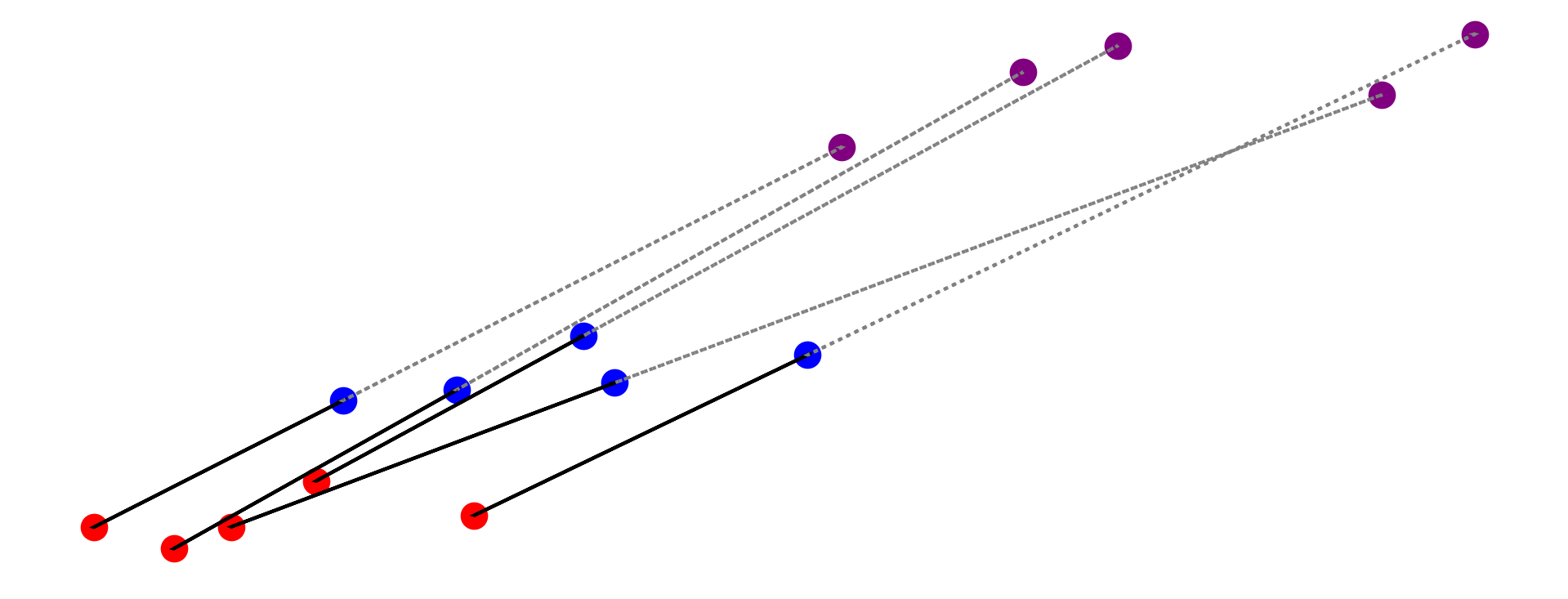
Thus, in essense, the approximation is computed by allowing the particles to evolve for a short time, relabelling the particles by , and then performing an Euler step for each individual particle using the derivative estimate given by the short time step. Figure 1 illustrates the approximation scheme in a simple case with 5 particles. The hope is that, up to a (possibly new) relabelling , we have
i.e., that is small.
It is important to point out that Corollary 12 requires that has density, which is not true in the discrete setting where it is an empirical measure. A tempting fix is to give each particle a local density, e.g., by setting
for some small variance . This does not resolve the issue, however: if the curve is not absolutely continuous in , then the curve is not absolutely continuous on the Wasserstein manifold, so Corollary 12 still does not apply. We are often concerned with the case where the particles are stochastic processes evolving according to some SDE, so the individual particles’ curves are nowhere differentiable and hence not absolutely continuous. Thus, the theoretical transition from the continuous case to the discrete case is not immediately obvious.
We will not fully resolve the theoretical hurdles in this paper, as work into making precise statements in the discrete case is still ongoing. However, we can still give a heuristic argument for why this approximation approach ought to work in the discrete setting as well. The fundamental problem with directly applying Theorem 11 boils down to the fact that there is no nice vector field that exactly describes the chaotic movements of the discrete particles at all times. However, if we allow the particles to evolve over a sufficiently long time, long enough that the long-term bulk behavior begins to overshadow the short-term particle behavior, then there is still a heuristic notion of a direction the particles as a group are traveling. The driving idea is that computing optimal transport maps allows us to access that heuristic.
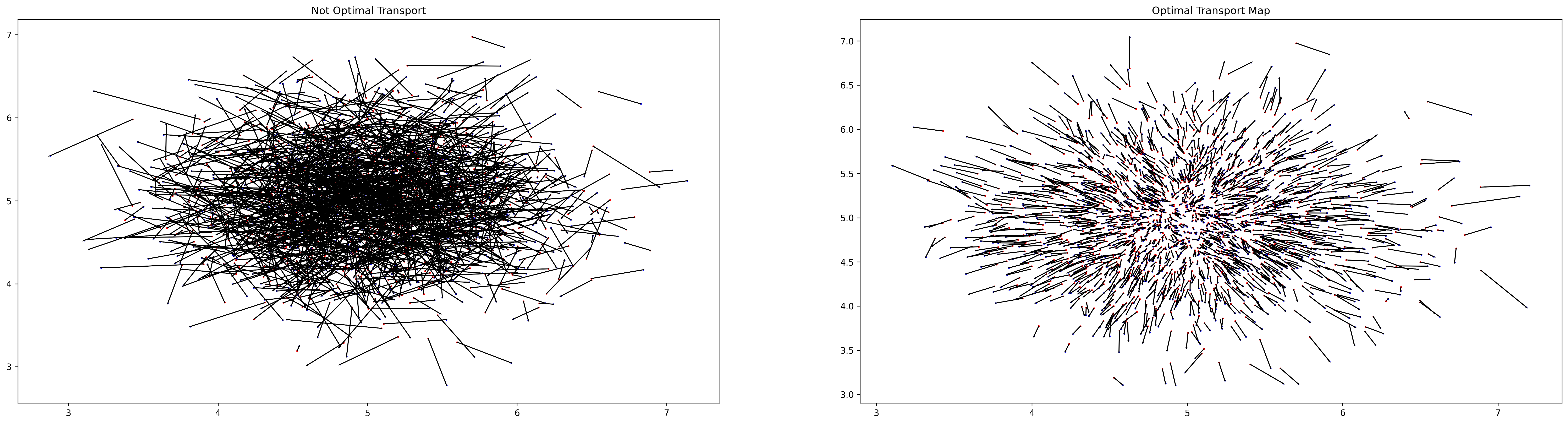
As an example, consider Figure 2. The first image shows 2000 particles evolving according to a standard Gaussian diffusion simulation (described in more detail in Section 5) for a short time, and an arrow drawn between each particle’s starting and ending location. The arrows are expectedly chaotic because the particles’ motions are individually unpredictable. In contrast, the second image shows an equivalent set of particles diffusing for the same amount of time, except instead of drawing the arrows particle-wise, we compute the optimal transport map from the beginning to the ending distribution. This map reveals an obvious structure in the distribution’s evolution: the distribution is slowly drifting away from the center in all directions, exactly the expected behavior of a Gaussian distribution diffusing over time. Even though the actual time derivatives are meaningless because Brownian motion is not differentiable, these finite differences over a slightly longer time step indeed give a reasonable approximation for a vector field that describes the distribution’s evolution.
The quality of the approximated distribution clearly depends on how well this discrete vector field captures the evolution of the overall distribution. In the continuous case, equation (6) says that the error in the vector field approximation, given by , decreases as decreases. This is a standard phenomenon in numerical approximations: the smaller the time step, the better the approximation.
In the discrete case, however, the fact that the particle-wise finite differences give a terrible approximation of the vector field (as seen in the first image in Figure 2) means there is a competing desire to keep sufficiently large in practice. More specifically, each is a continuous curve in , so choosing small enough will make , and then the vector field produced by the optimal transport map really is just a particle-wise finite difference approximation of each particle’s velocity. We know that this particle-wise construction does not accurately depict the overall flow of the distribution, so this means it is possible to choose too small.
To strike a balance between short steps (which give more accurate finite differences) and longer steps (which allows the bulk behavior to manifest more clearly), we propose a scheme in which we take an average of finite differences computed with a range of different time steps over some interval. If we consider the middle of this interval to be the time at which we are hoping to approximate the derivative, then taking an average of both forwards and backwards differences becomes equivalent to taking an average of centered differences. Explicitly, for a fixed time step and discrete times , we set
Note that the last line is the average of centered-difference approximations of centered at and with time steps . This is the method we use in practice.
This method for approximating the derivative works well on toy examples where the vector field is explicitly calculable in theory (e.g., diffusion), and the associated projection scheme described by (10) gives reasonable predictions for the overall distribution. As we will see in Sections 5 and 6,
gives a reasonable approximation for the actual distribution in some standard particle system examples.
4.1 Iterative Approximations
The discussion in Section 3 about the distribution evolving linearly is of particular interest when the goal is to approximate the particles’ behavior for a very long time (e.g., if the goal is to approximate the steady-state distribution). Even extremely simple examples of SDEs (e.g., diffusion) do not satisfy the linearity condition (9), which means one extremely long time step will be wildly inaccurate. Instead, it is more accurate to take a number of smaller steps, much in the same way that taking smaller time steps is generally more accurate when numerically approximating solutions to ODEs. This requires the ability to allow the distribution to continue evolving “naturally” after taking a step forward in order to compute to use in the computation of , and so on. This may be difficult if the particles are some physical objects, but it is trivial if we suppose the “true” evolution of the particles is given by some micro-scale model. With a micro-scale simulation, we can simply re-initialize the positions of the particles to be those of and start the simulation again, gather new derivative estimates, and then step forward again to approximate . For this reason, we henceforth only consider particle systems for which we have a known micro-scale model, and we consider the result of running the micro-scale simulation as the true curve .
One potential hurdle with the approach of taking multiple steps and re-initializing particle locations after each, however, is that the approximated distribution will be slightly different than the true distribution, and running the micro-scale simulation on the approximated distribution might result in behavior that is initially dominated by the approximated distribution returning to a relative equilibrium. To account for this, and to make sure the approximated derivatives are capturing mostly the long-term dynamics, we must allow the approximated distribution to evolve according to the micro-scale simulation for a prescribed duration before starting to take samples to use in the computation of .
4.2 Approximation Algorithm Procedure
Putting everything together, the overall scheme for approximating the distribution for large is as follows. We fix values for the parameters
| the time of one step of the micro-scale simulation | ||||
| the number of centered differences to average | ||||
| half the length of the derivative-sample time window | ||||
| the length of each approximating step | ||||
| the recovery time after each approximating step | ||||
| the time difference between approximations |
and then do
-
1.
Run the micro-scale simulation for some start-up time to allow the initial distribution to reach a relative equilibrium (if necessary).
-
2.
For each approximating step :
-
(a)
Take micro-scale steps and compute for each in .
-
(b)
Set .
-
(c)
Take micro-scale steps to allow the distribution to recover.
-
(a)
-
3.
Run the micro-scale simulation for some final recover time to ensure any fringe errors in the approximations are minimized (e.g., that the distribution has indeed reached a true steady state).
The above scheme reduces the number of micro-scale steps required to reach the desired end time (as compared to equivalent simulations that only use micro-scale steps) by a factor of , so ideally we would like to have so that the speed-up is nontrivial. Experiments on some toy examples (Sections 5 and 6) demonstrate that, with well-chosen values, the above scheme works well to predict long-term behavior of distributions while also giving meaningful speed-up.
Another hurdle with this scheme is that it only gives a way to approximate future locations of particles. This means that, strictly speaking, this scheme only works for particle clouds that evolve according to position-dependent micro-scale simulations, for example, Euler-Maruyama models of the form
where . Since micro-scale models of this form are time-independent, nothing needs to be updated between predicting steps, i.e., between steps 2(a) and 2(c) of the above algorithm. However, if the micro-scale model depends on anything other than the position of the particle, then this data must also be predicted across the predicting step taken in step 2(b) above. In general, there is no particular method for doing this, but we will discuss ad hoc approaches as they come up in Section 6.
5 Diffusion
5.1 Diffusion in One Dimension
To evaluate how well the approximation scheme described in Section 4 performs in practice, we compare the approximations with an actual numerical simulation of the distribution evolution. We model standard Brownian motion in one dimension by the Euler-Maruyama numerical scheme
where are i.i.d. and for some small time step . If we consider to be independent samples from an initial distribution , then the empirical distributions
give an empirical estimate of the distribution , where is the law of the solution to the SDE
at time . To ensure that this system approaches a steady-state that has positive density, we consider the case of Brownian motion in a bounded domain . To achieve this numerically, we add the condition that if is outside the allowed domain, then we reflect it across the nearest boundary (and repeat if necessary). For example, if , then we set
The steady-state distribution is then the uniform distribution on .
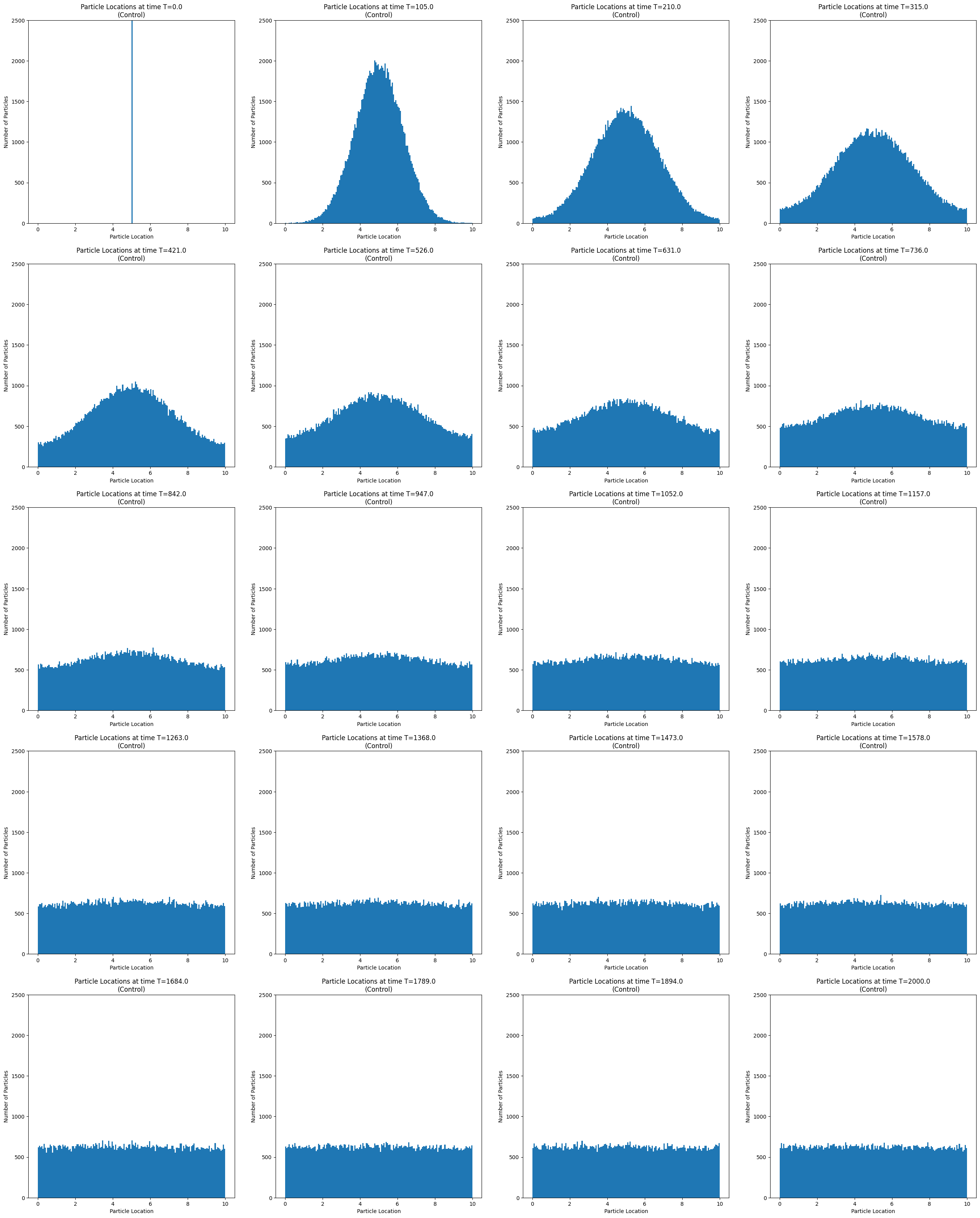
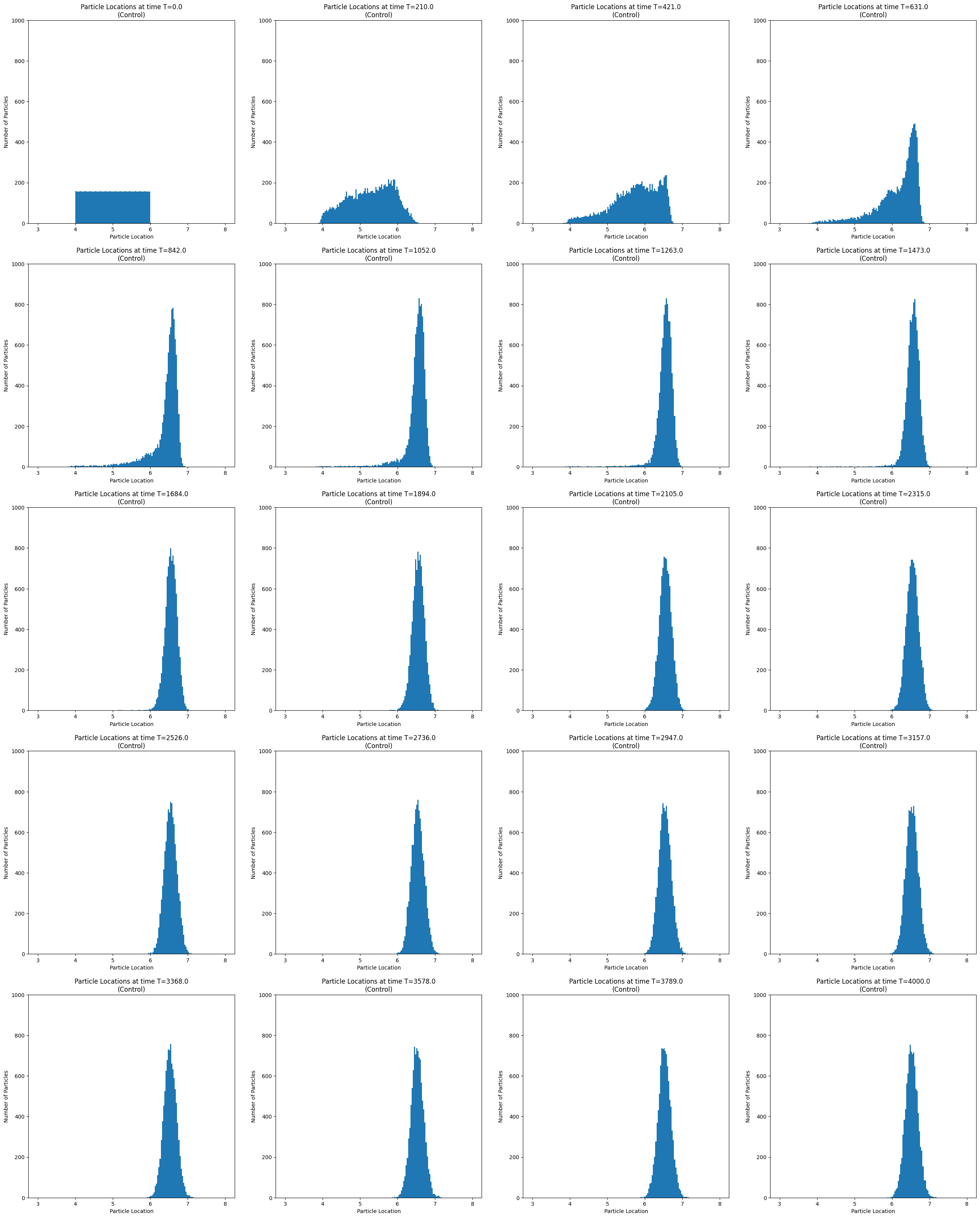
Before we run the approximation scheme, we first run the above diffusion micro-scale simulation from to with the parameters shown in Table 1. Figure 3 shows histograms of the particles over time. We consider this data to be the “control” data, and we will compare the results of our approximation algorithm against these control distributions.
| number of independent particles | |
| micro-scale simulation step size | |
| particle “speed” | |
| initial particle locations | |
| domain bounds | |
| end time |
We then run the approximation algorithm with the same parameters as above (Table 1) and the following additional parameters (as defined in Section 4):
| length of start-up time | ||||
| number of centered differences to average | ||||
| length of each big approximating step | ||||
| recovery time after each approximating step | ||||
| number of approximating steps | ||||
Note that the total length of this simulation, then, is
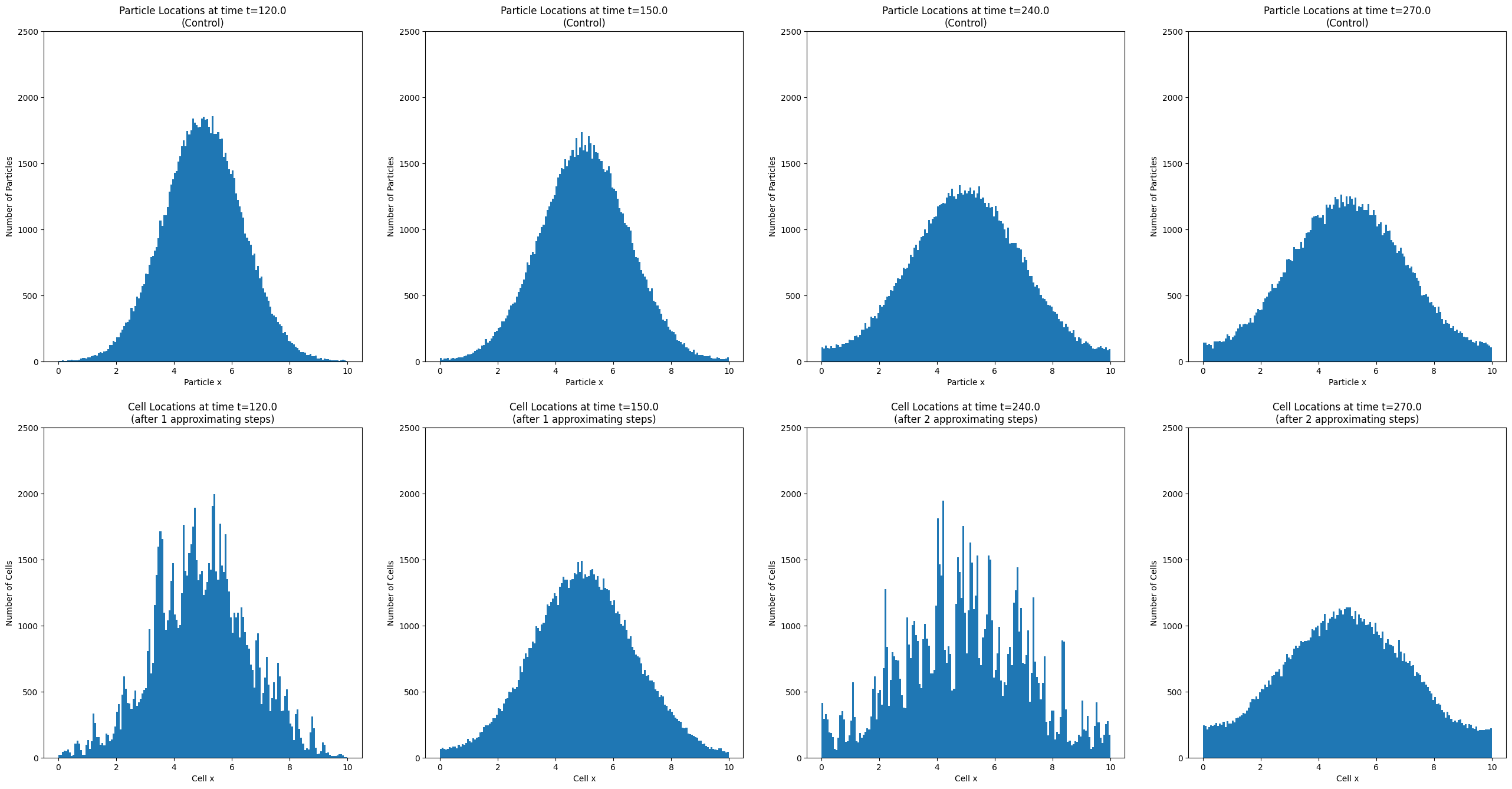
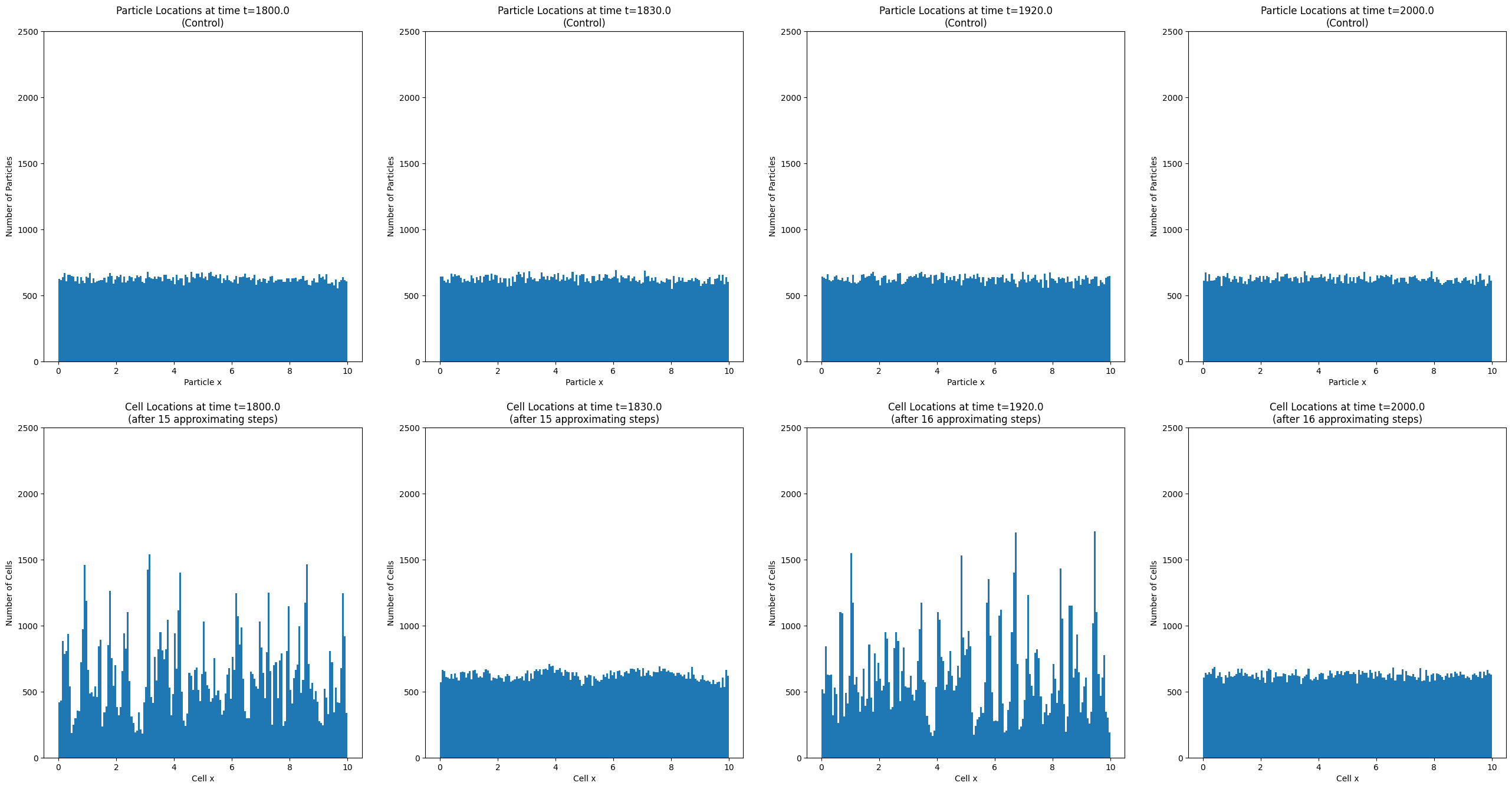
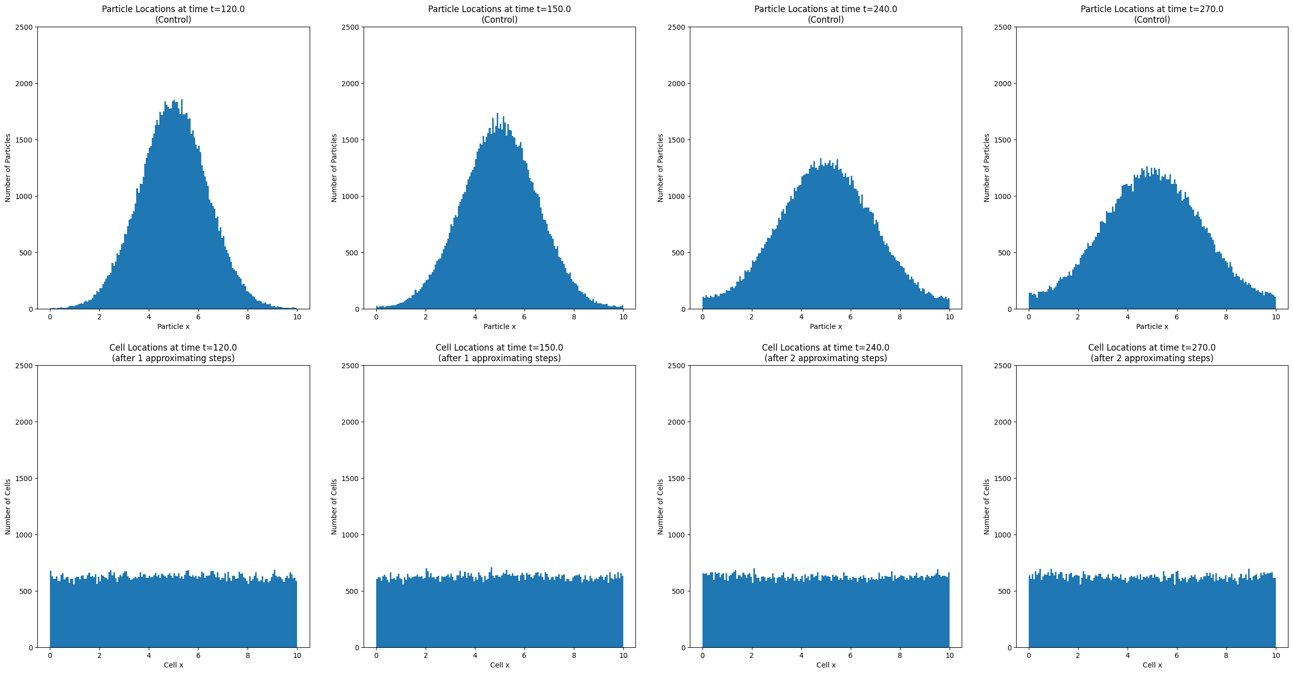
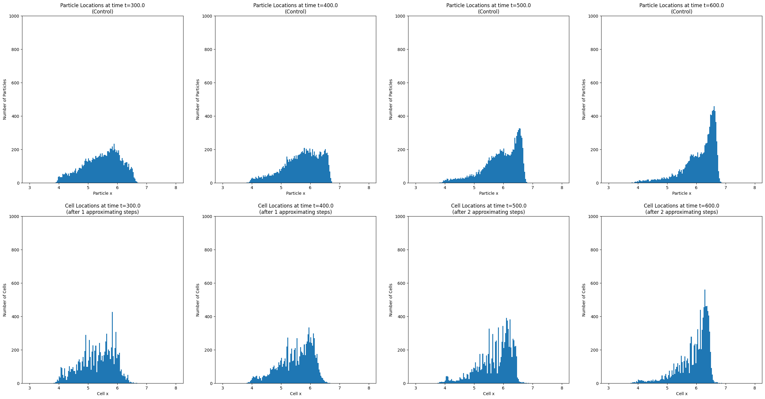
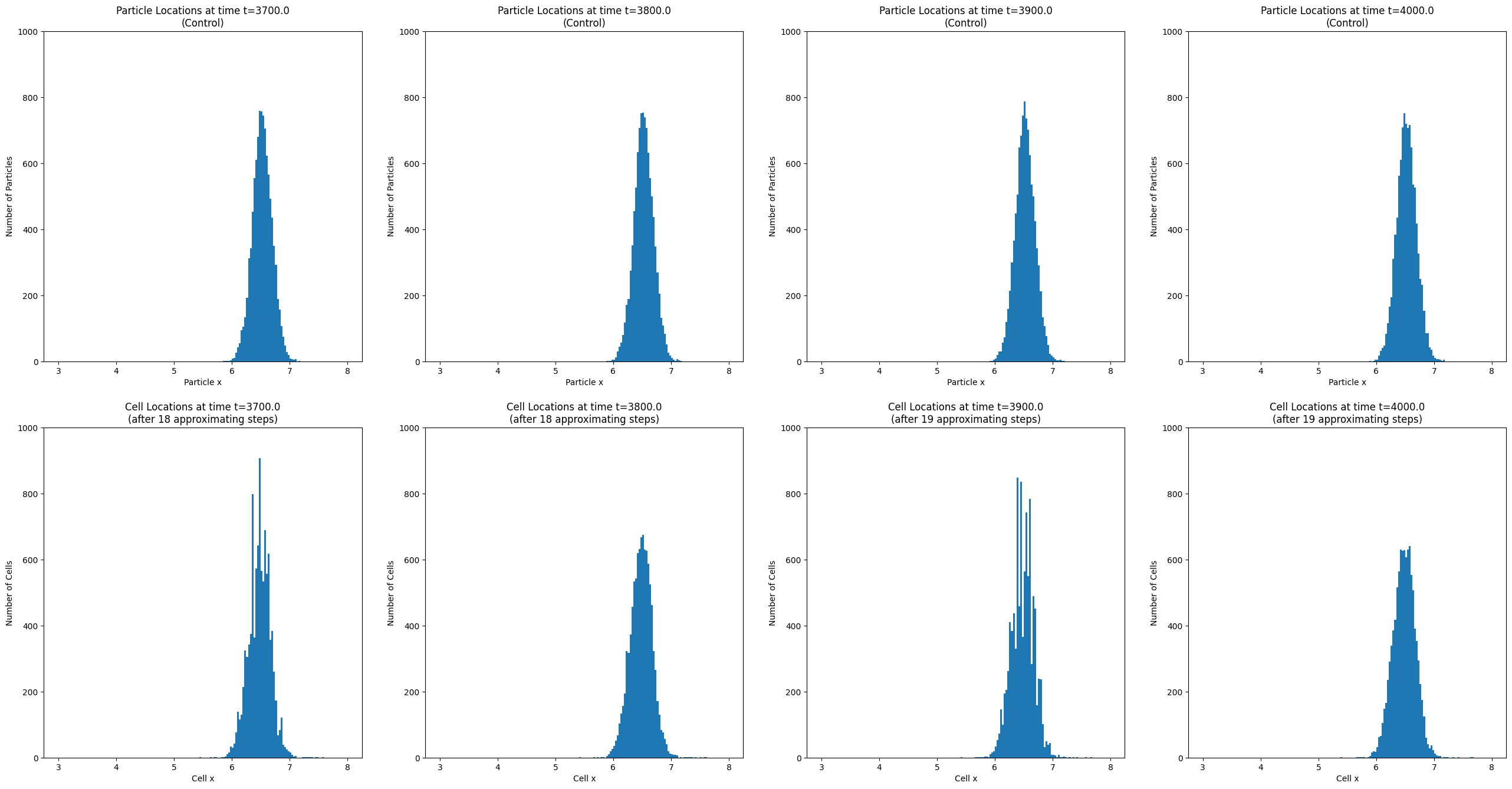
Figure 4 shows the distributions obtained after the first two approximating steps (), the distributions after the s recovery time (), and the distributions from the control simulation at the corresponding times for comparison. Similarly, Figure 5 shows the last two approximating steps () and corresponding recovery times ( — recall that the last recovery time has an additional s). In both figures, we notice that the distributions immediately after the approximating steps look very different than the control distributions at the corresponding time. This is exactly why the recovery time is critical: if we started approximating derivatives immediately after the approximating step, the short-term behavior would be dominated by the distribution returning to a smooth Gaussian, and the longer-term diffusion behavior would be masked.
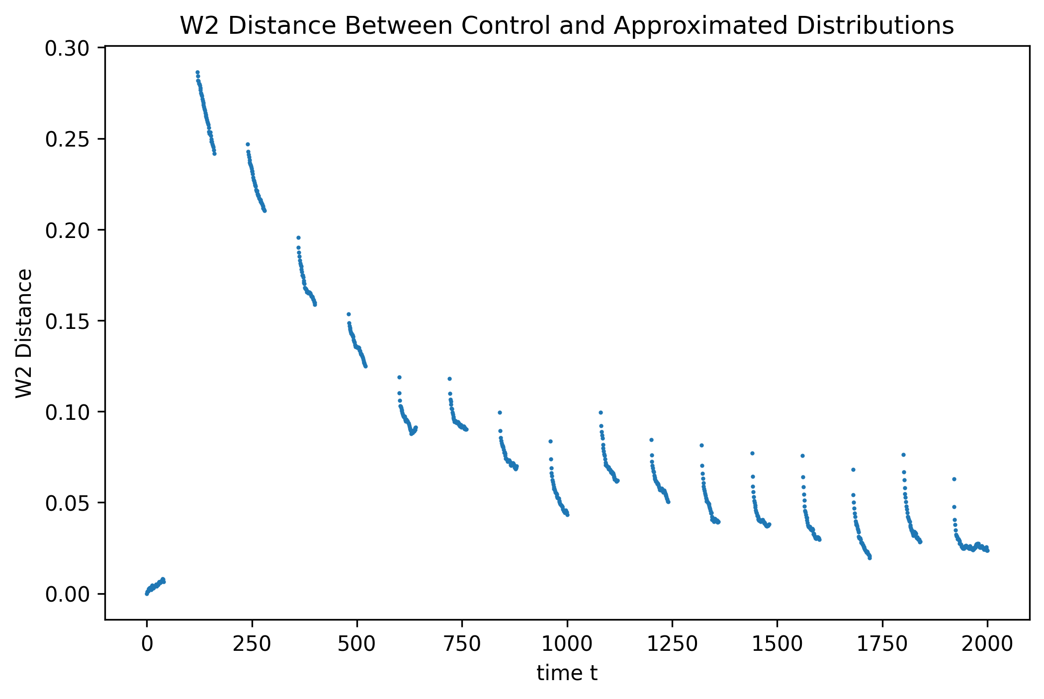
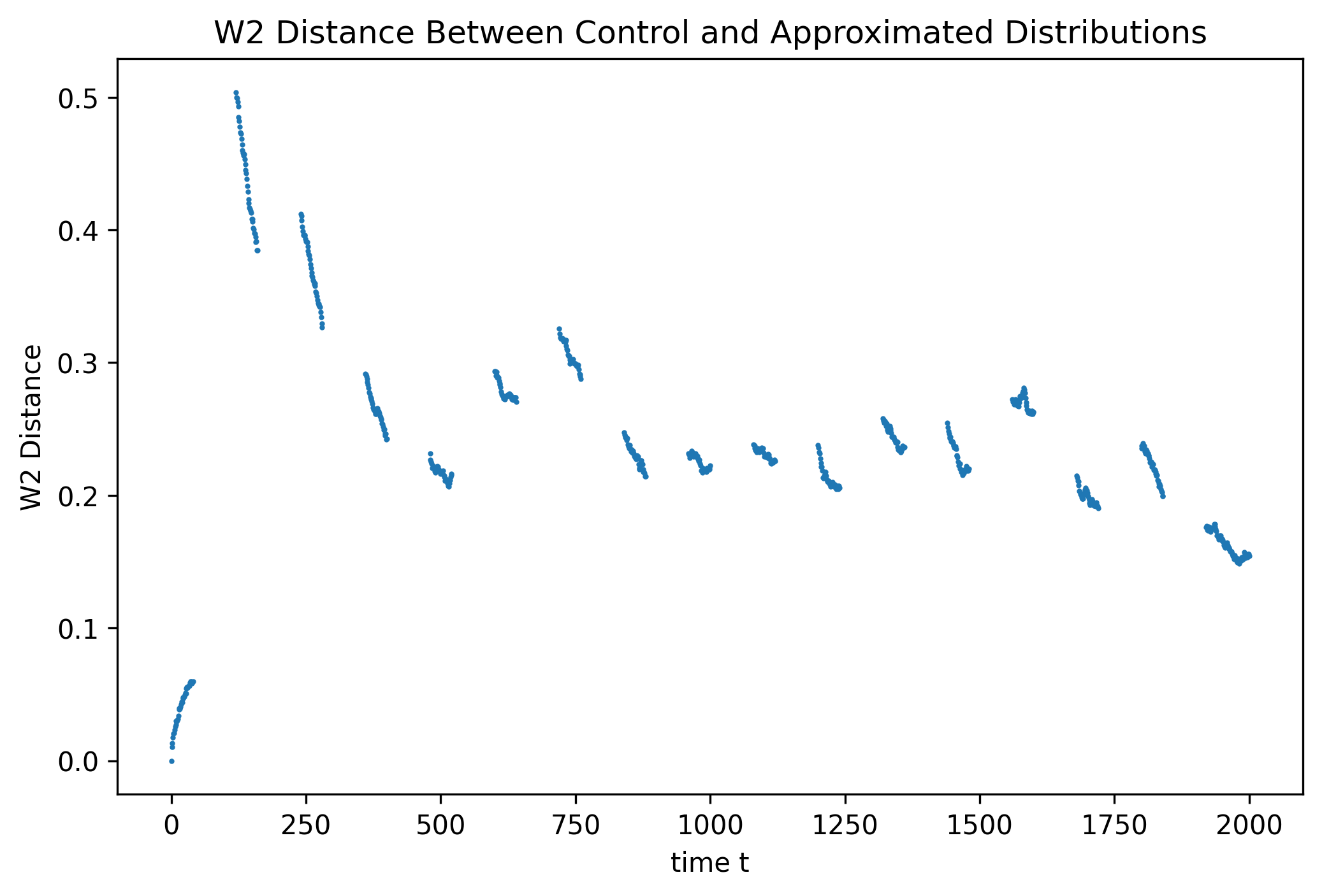
We can quantify this behavior by computing the distance between the control distribution and the approximated distribution at all times . A plot of versus time is shown in Figure 6. We see that the distance rapidly decreases immediately after each approximating step, but the rate of decrease slows considerably after a short time. This corresponds to the distribution having “recovered” as much as possible, at which point the long-term dynamics are once again dominating the behavior of the distribution. Accurately determining when this occurs is critical to selecting an optimal value for the duration of this recovery window. Our current approach is to pick this value based on observed experimental data, but one could devise other algorithms that adaptively determine the recovery time.
This discussion ignores the perhaps even-more-pressing question at hand here: why are the histograms immediately after the approximating steps so spiky? To explain this phenomenon, it is helpful to reframe our perspective. Instead of considering each point and determining where it goes after the approximating step, we should consider which points get sent to within of a fixed point after the approximating step. The approximating step is computed by the map
so a particle gets mapped to within of exactly when
This means we can compute
Note that is an affine condition that describes a strip of the -plane with slope . This means the total mass that gets sent to within of is the total mass that lies in this strip of the -plane. The spiky distribution behavior, then, occurs when there is a large total variance in the amount of mass that appears in each of these strips. Investigating methods for smoothing the curve to hopefully reduce this effect is another direction of active study.
We can also see from Figure 6 that final approximated distributions between and (during the longer final recovery time ) have an approximately constant distance from their respective control distributions. Since the control distributions have reached steady state by then, this indicates that the approximated distributions have also reached a steady state. The histograms of these distributions shown in Figure 5 confirm this.
Overall, with the parameters described above, the algorithm only requires 1/3 as many micro-scale steps as the control simulation (10 seconds of derivative-approximation and 30 seconds of recovery for every 120 seconds of simulated time). A natural question is whether we can achieve a better ratio while retaining the accuracy in approximations. The three ways to do this would be to decrease the derivative-approximation window , to decrease the recovery time , or to increase the approximation step size . We will address each of these separately.
We discussed ways to decrease the recovery time in Remark 5.1, and Figure 6 hints that we could only do marginally better before impacting accuracy (and we have empirically verified this by otherwise equivalent experiments with shorter recovery times). So with the specified parameters above, seems to be approximately optimal.
Decreasing the derivative window has a similar story. We have observed that the approximation accuracy also noticeably decreases with any substantial decrease in . It is also important to point out that is considerably smaller than , so even decreasing to 0 while keeping fixed would only improve the micro-step ratio to 1/4. The biggest improvements will come from decreasing or increasing .
The last way to achieve a better speed-up ratio is to take larger approximating steps by increasing . Any discussion about how far we can reasonably step and still get an accurate approximation quickly becomes a discussion about the appropriate notion of a second derivative and what it means to “evolve linearly,” which is discussed in broad terms in Section 3. However, we can get a good visual understanding of whether the system is evolving linearly by doing a dimension-reduction on the OT maps. Since OT in one dimension can be solved explicitly in terms of CDFs, then for any fixed distribution with particles (e.g., the uniform distribution on ), we can compute the map by simply sorting the particles’ locations at time . This means we get a universal embedding of the transport maps at each time . In particular, we can perform PCA on , where is the -dimensional vector of sorted particle locations at time .
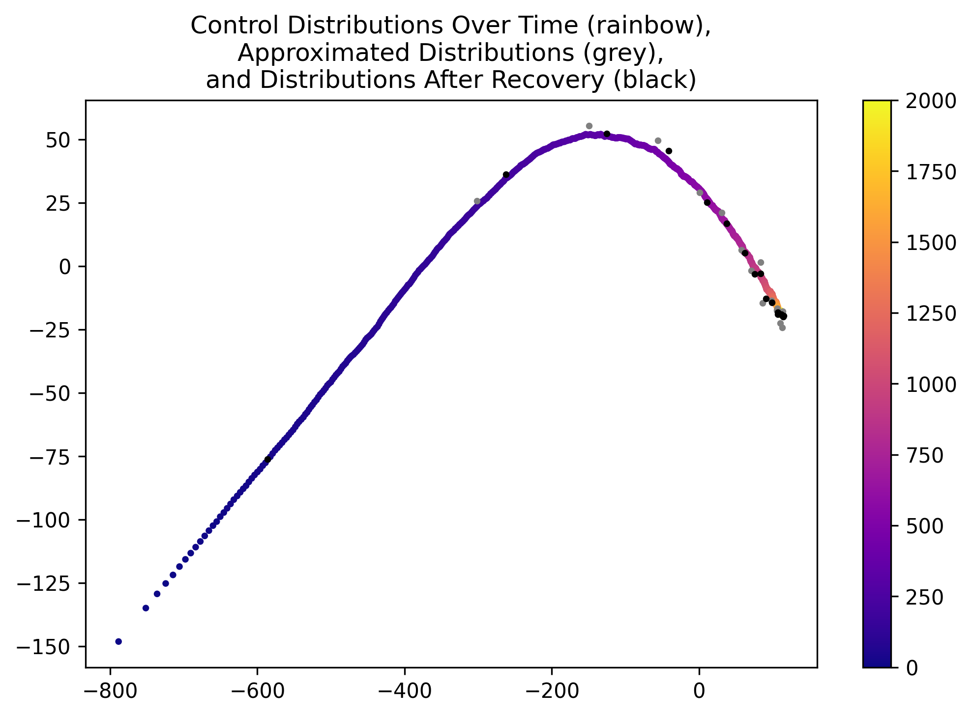
Since this embedding is universal, we can compute the PCA embedding of both the control distributions and the approximated distributions . The projection of these distributions onto the first two principal components is shown in Figure 7. This image gives a good heuristic argument that the distribution is indeed evolving “linearly” in the sense that the OT maps are following a trajectory that appears to have small second derivative at most times. Of course, data is lost in the dimension reduction, but the global evolution of the distribution appears to be very smooth. Moreover, the plot indicates that the approximating step size is small enough that it places the approximated distribution (grey dots) very near the control curve, but it also indicates that stepping much farther in that direction would quickly lead to the approximations being considerably farther from the control curve, especially for the first few approximating steps. Later steps could be longer since the distribution is close to the steady state, and hence the derivative of the optimal transport maps is very small. With small derivative, even large steps would not result in a large change. However, if we require a fixed approximating time for all steps, then is approximately optimal. As discussed in Section 3, the optimal step size should be a function of the “second derivative” of the curve, so a direction for future work is to attempt to dynamically adjust the length of this step based on an appropriate estimate of the second derivative.
5.2 Diffusion in Two Dimensions
While similar work with sorting particles has been explored before (e.g., [30]), one of the advantages to framing this prediction algorithm in the context of optimal transport is that it easily generalizes to higher dimensions. In fact, Corollary 12 does not depend on the ambient dimension (although it is reasonable to expect that the constants in the convergence rate depend on the dimension). To empirically verify the claim that this approximation scheme is effective in higher dimensions, we perform exactly the same tests with diffusion in two dimensions. Explicitly, the control simulation is governed by the micro-scale Euler-Maruyama scheme
where are i.i.d. We use exactly the same parameters for the control simulation as in 1-D, except we decrease the number of particles for computational reasons explained later:
| number of independent particles | |
| micro-scale simulation step size | |
| particle “speed” | |
| initial particle locations | |
| domain bounds | |
| end time |
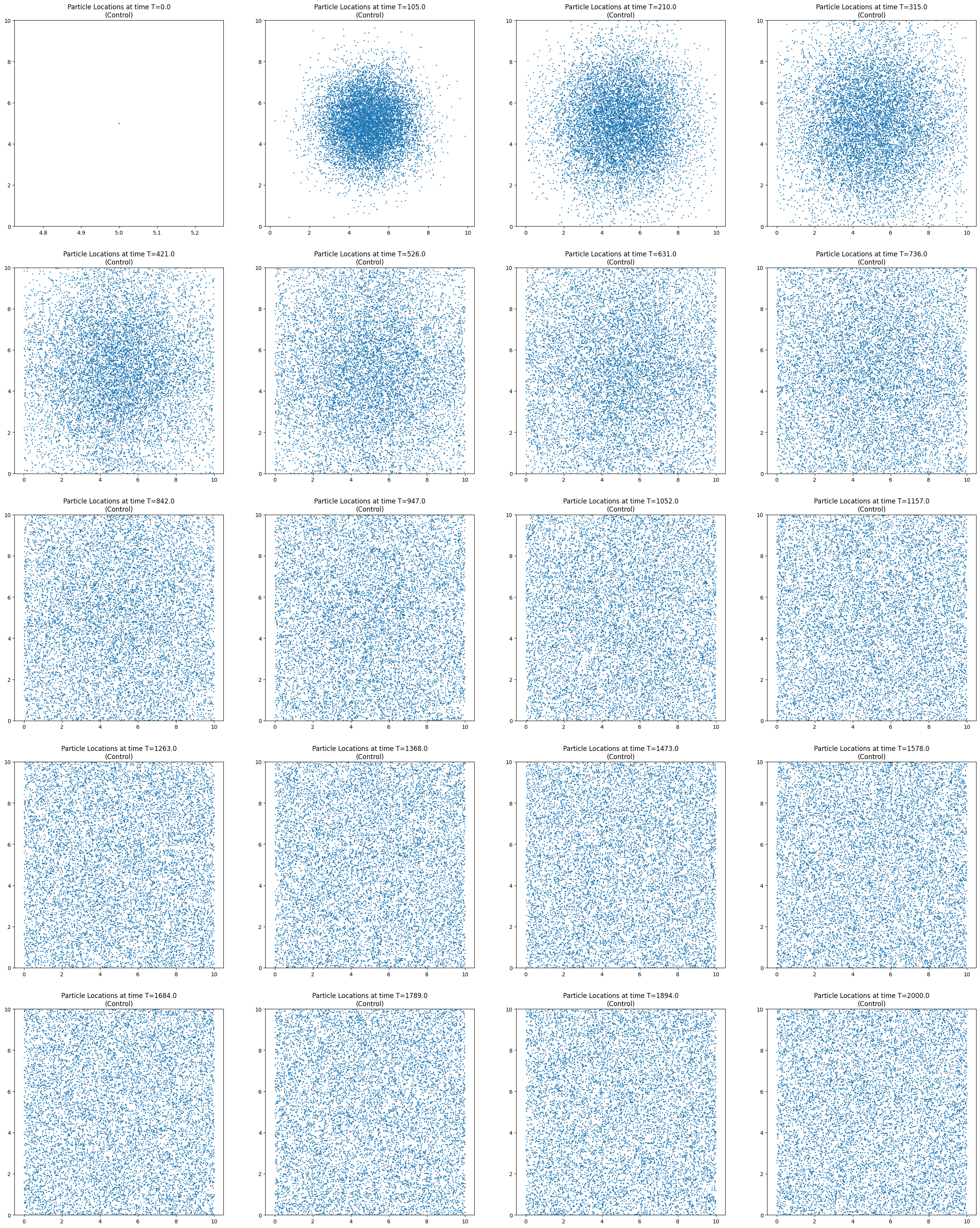
Figure 8 shows scatter plots of the particle locations over time, which we again take to be the control data. We then run the approximation algorithm, also with the same parameters as in the 1-D case:
| length of start-up time | ||||
| number of centered differences to average | ||||
| length of each big approximating step | ||||
| recovery time after each approximating step | ||||
| number of approximating steps | ||||
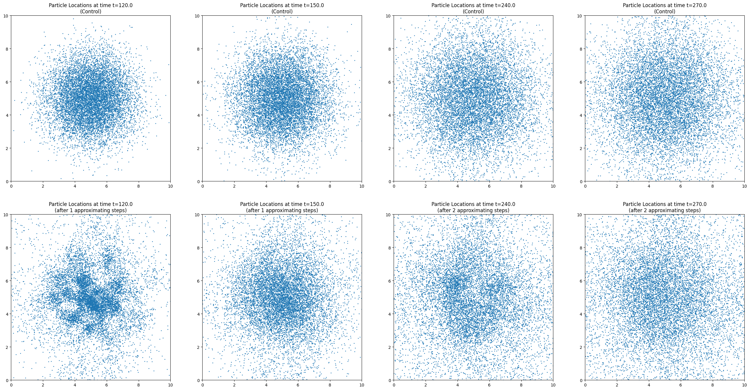
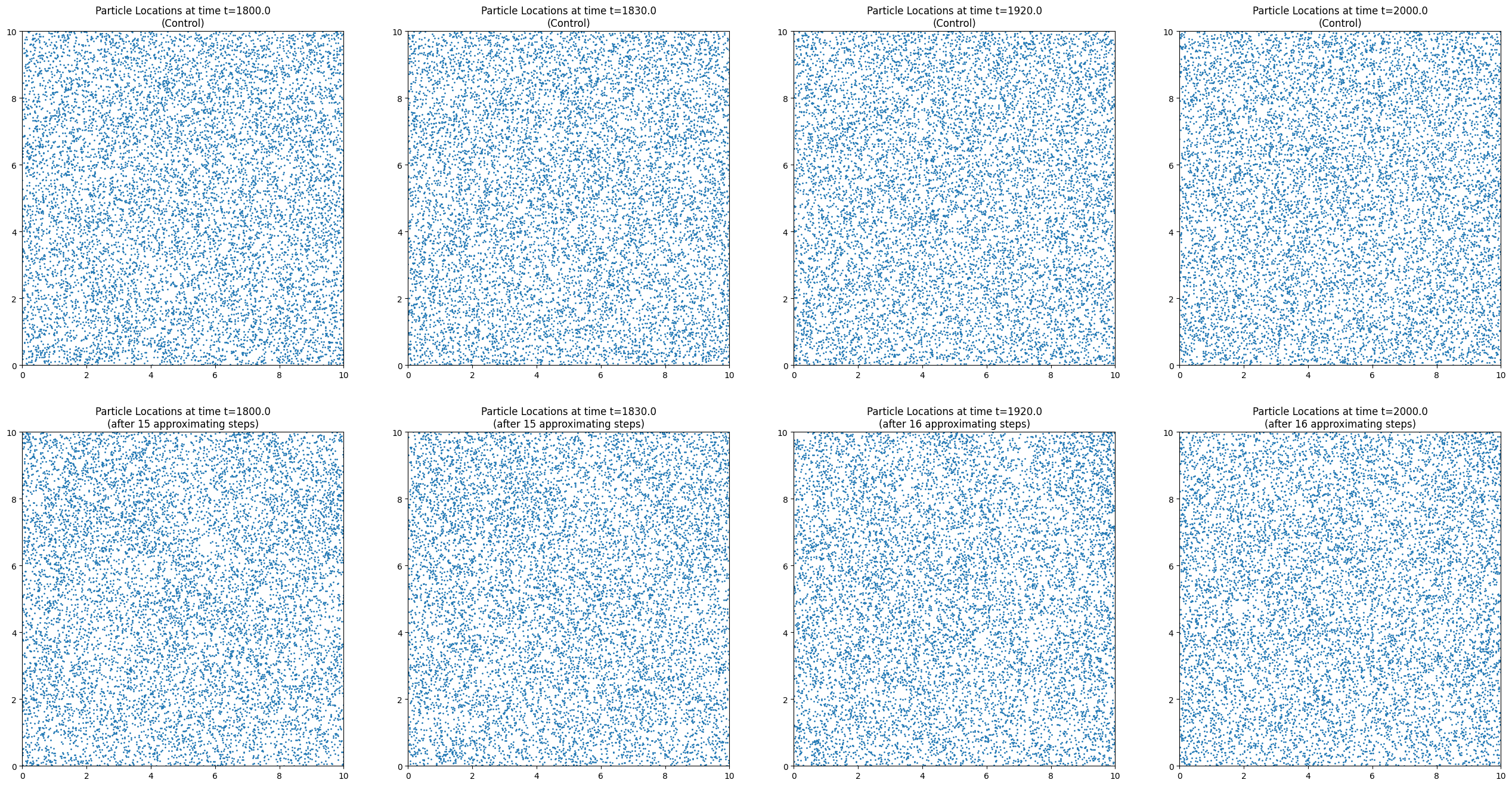
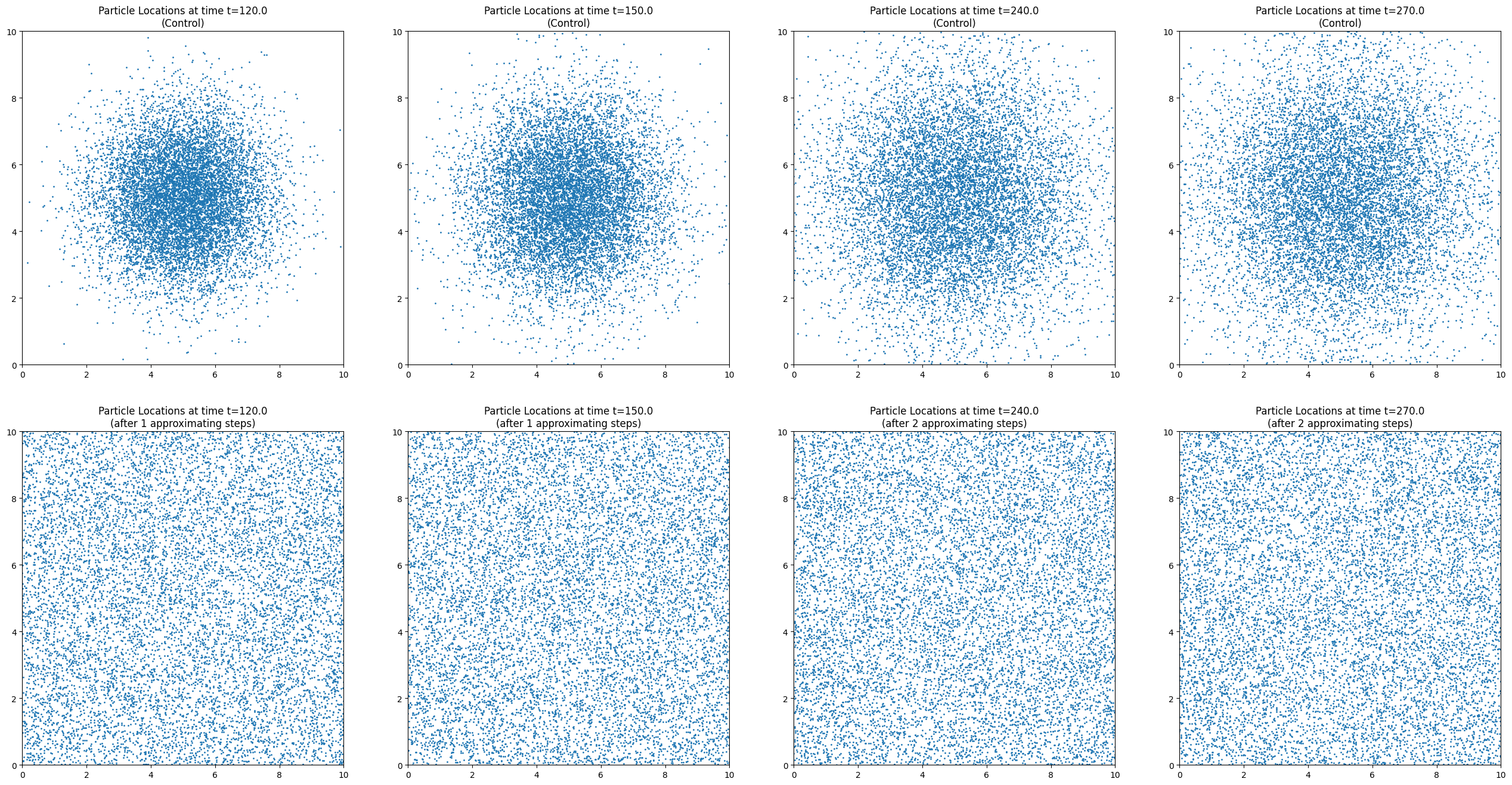
Figures 9 and 10 show the results of the first two and last two approximating steps, respectively, both before and after the 30s recovery period. We once again notice the concentrating behavior in the distributions immediately after the approximating steps, especially in the first two, and this is corroborated by looking at the distance between the approximated and control distributions plotted in Figure 11.
While this experiment suffers slightly from the reduced number of particles (which we believe to be the cause of the increase in noise of the approximations), it demonstrates that the approach is just as sound in two dimensions as it is in one. Unfortunately, the cost of computing the optimal transport maps in higher dimensions is much greater. In one dimension, sorting the particles is sufficient, so the cost is of order . In higher dimensions, computing the optimal transport map involves solving a linear program222We use the Python Optimal Transport (POT) library for computing optimal transport maps in the 2-D experiments., which is of order [8]. This significant increase in computational complexity is the reason for the decrease in number of particles in the 2-D experiment. Since we need to compute optimal transport maps per approximating step, it was necessary to reduce the number of particles in the simulation in order to keep run times reasonable.
5.3 Comparison with Particle-wise Approach
To see the benefit of using optimal transport, we compare the above experiments to the equivalent experiments without using OT, i.e., by keeping track of individual particles, attempting to approximate their derivative, and then taking an Euler step in that direction. Explicitly, instead of approximating by using
we could instead attempt to approximate simply by computing
effectively attempting to approximate (ignoring the fact that this derivative does not actually exist for particles evolving according to Brownian motion). This approach is extremely similar to the optimal transport approach, except we do not relabel any of the particles. As described in Remark 4, we can think of the optimal transport map as relabelling each particle in the target distribution based on which particle in the reference distribution most likely moved to become that particle, but if we ignore the relabelling process, we simply get an approximation for the velocity of each individual particle. Intuitively, this should give a much worse understanding of how the overall distribution is evolving, and indeed this is exactly what the experiments show.
We perform exactly the same experiment with the same parameters as above, with the only change being how we compute the velocity field . Figures 12 and 13 show the result of the first two approximating steps in 1-D and 2-D, respectively, using the particle-wise approach to compute . We see that the approximated distribution immediately becomes uniform and does not match the corresponding control distribution at all. This shows that the optimal transport maps are an essential component of this prediction algorithm.
In the case where is differentiable for all , we can interpret
as approximating . In order for this to give an accurate approximation, we need to be an accurate approximation of , which may yet hold under some conditions. In particular, this approximation becomes better as each particle’s behavior becomes more deterministic. Thus, the more chaotic each particle’s motion is on short time scales, the greater the advantage is to using optimal transport over making predictions particle-wise.
In the case of diffusion, it is easy to understand why the particle-wise estimate of the vector field does not capture the correct bulk behavior at all. For any individual particle, its average velocity from to is a normal random variable with mean 0 because it is simulating a standard Brownian motion. In particular, the estimate for its velocity vector is independent of its current position, which means there will be no structure to the vector field created by computing particle-wise velocities. However, we know analytically that the bulk distribution evolves according to a nonzero vector field — the distribution slowly spreads out over time. This spreading-out movement is the evolution that we want the vector field to pick out, and indeed it is the structure that the optimal transport map captures (see Figure 2), but it is completely unrelated to the expected motion of the individual particles.
6 Chemotactic Mobility of Bacteria
6.1 Problem Setup
The diffusion experiments described in Section 5 have a simple property where the micro-scale simulation only depends on the locations of the particles. This time independence allows us to approximate large-time steps within reasonable error bounds. However, some micro-scale models, such as bacterial locomotion by chemoattractant, are intertwined with other spatiotemporal variables, like a chemoattractant profile. As a result, a proper re-initialization of the micro-scale properties at the predicted location is required for an approximation of a large-time step of all dependent variables, leading to a challenging problem.
In order to demonstrate the effectiveness of the suggested approximation algorithm in a complex micro-scale simulation, we have applied the method to a biological application — the chemotactic movement of bacteria. The mobility of bacteria is affected by the presence of chemoattractant (specifically, its spatial derivative). However, when we approximate the location of bacteria after a large time step, we may lose the actual trajectory of the bacteria due to a lack of information about the chemotactic effect, resulting in inaccurate predictions. If the chemoattractant profile is smooth enough in space, the microscopic properties of bacteria can be re-initialized within a short recovery time and then follow slow dynamics.
The chemotactic mobility of bacteria has been simulated using a microscopic and stochastic simulator [30, 20]. In this paper, we provide a brief description of variables and a summary of the setup for this micro-simulator. For more theoretical and technical details, please refer to the cited papers.
Here are brief descriptions of the variables in the micro-simulator we discussed in this paper as follows:
-
•
: the number of bacteria (the number of simulations).
-
•
: -dimensional position vector for each bacteria.
-
•
: indicator of rotating direction of flagella, clockwise or counterclockwise. If more than three flagella are rotating counterclockwise, bacteria start moving.
-
•
: microscopic time step
-
•
: the swimming speed of each bacteria
-
•
: chemoattractant profile
For reference (ground truth), we run the simulation without prediction to establish a “control” as the ground truth behavior of the system. We use the same parameters as in [30, 20] with only the following changes:
| number of bacteria | ||||
| microscopic time step | ||||
| swimming speed of bacteria | ||||
| chemoattractant profile |
Histograms of bacteria positions at different times in the control simulation are shown in Figure 14.
To simulate the next time step, the micro-scale simulator requires not only current bacteria locations but also all microscopic quantities. However, the suggested algorithm described in Section 4 predicts only the locations of bacteria after the next approximating step, resulting in a lack (or missing) of microscopic quantities. Hence, after the approximating time step, the suggested algorithm requires the re-initialization step of microscopic quantities, such as , and . Even though some (quantitatively not but) qualitatively good re-initializations quickly reach slow dynamics, we suggest a better re-initialization scheme based on the history of microscopic quantities and demonstrate a more accurate prediction of bacteria density distribution over multiple approximation steps, see the following sections.
6.2 History-Dependent Re-initialization Scheme
To compare with the control data, we perform a simulation using the approximation algorithm with the following parameters:
| length of start-up time | ||||
| number of centered differences to average | ||||
| length of each approximating step | ||||
| recovery time after each approximating step | ||||
| number of approximating steps | ||||
After each approximating step, we re-initialize the underlying data according to the history-dependent scheme in Table 3. For example, given data at time , we use the optimal transport approximation scheme to predict the bacteria locations at , and re-initialize the microscopic properties at as follows:
-
•
set for all bacteria
-
•
compute from the prescribed ODE in [30] to take an Euler forward step
-
•
keep the flagella rotating direction and bacteria moving direction exactly the same as they were at time .
6.3 Comparison with Different Re-initializations
To demonstrate the effectiveness of the suggested re-initialization, we also perform a history-independent re-initialization as described in [30]. Table 3 shows the different parameters of re-initialization between the two schemes. In Figure 17, we provide a comparison of the distance between the control and approximated distributions over time for the two different approximation schemes.
| Parameters | History-Dependent Scheme | History-Independent Scheme |
|---|---|---|
| (fixed) |
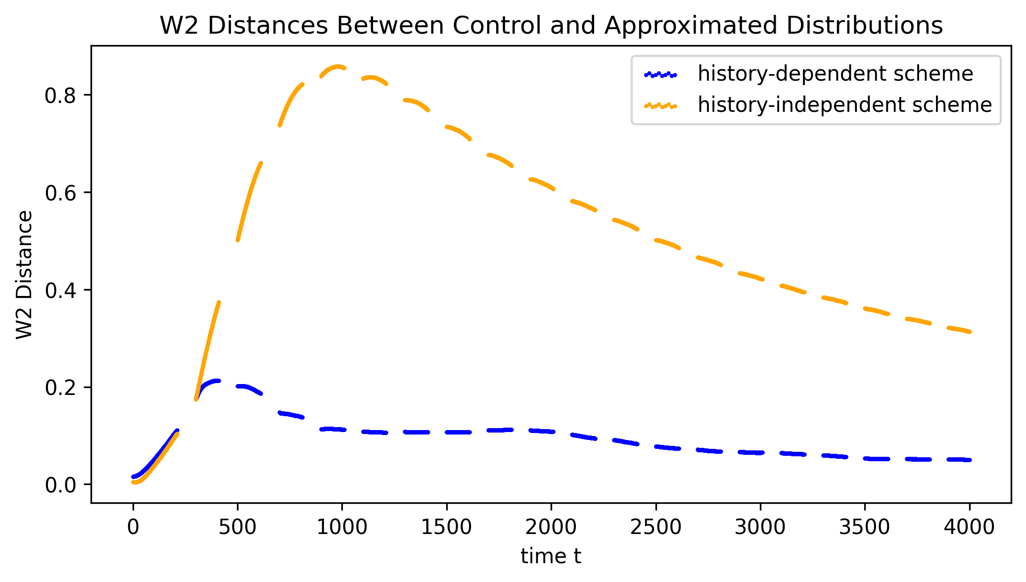
The first approximating step shows similar results between the two experiments while the history-independent scheme becomes (qualitatively good but) “relatively” inaccurate by the end of the first recovery period. This is because the history-independent method re-initializes the microscopic properties with a “fixed” value regardless of current conditions, resulting in a large recovery time to reach slow dynamics while the history-dependent scheme uses the current microscopic properties to re-initialize the next approximating step. In other words, the underlying variables (particularly and the flagella rotating direction) could not respond quickly enough to the fixed re-initialization. Furthermore, even though the distributions look the same after the first approximation step, the two methods still yield different subsequent microscopic behavior, leading to slightly different slow dynamics.
The observation in Figure 17 suggests that the underlying microscopic properties are important components in the micro-scale simulation. Hence, different settings of the properties result in different overall distribution behavior. In the language of Section 3, the vector field that describes the distribution evolution is somehow a function of these variables, not merely a function of position, so the method we choose to predict them across approximating steps is critical to our capability to approximate the evolution using optimal transport maps.
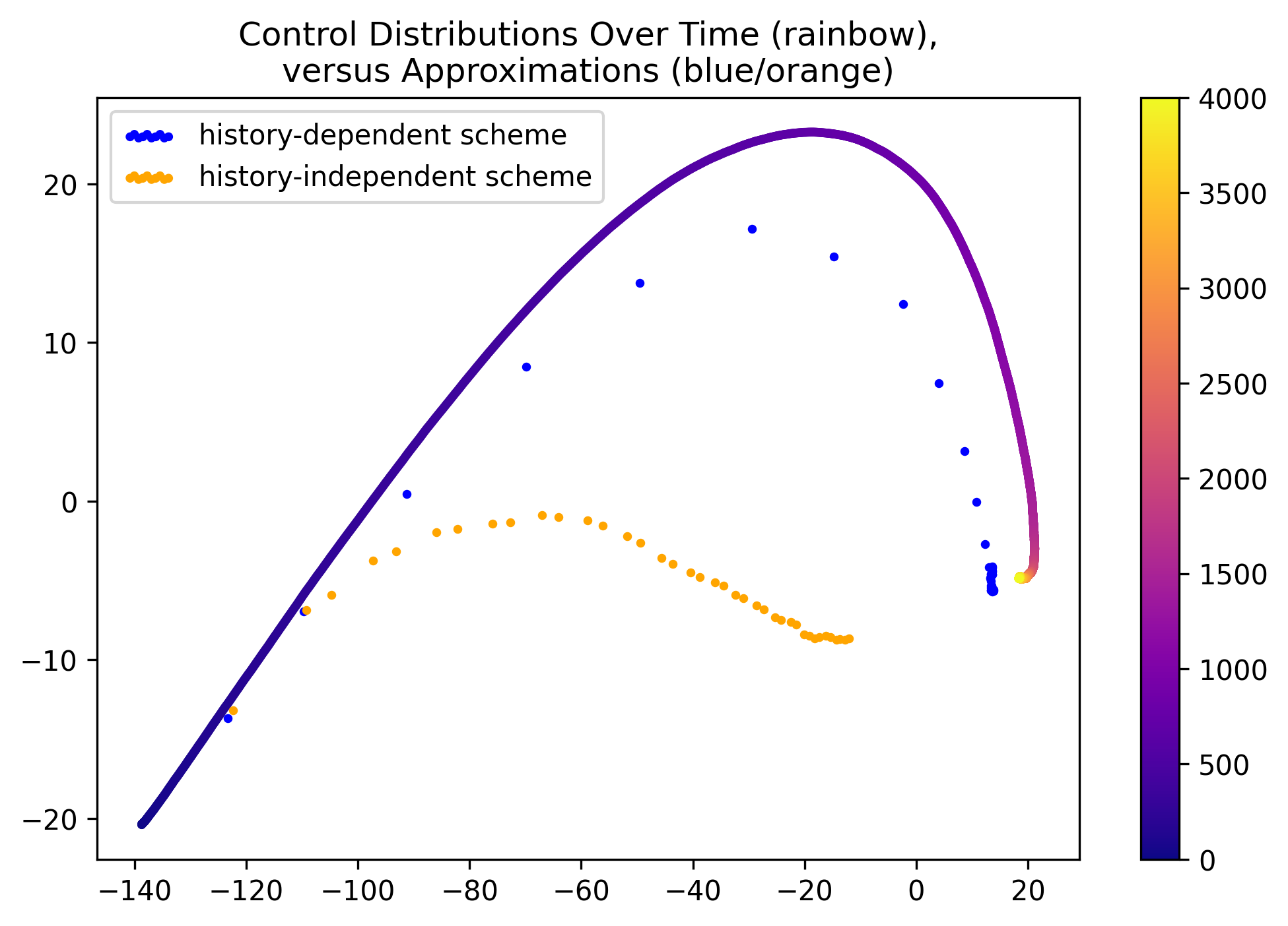
We demonstrate that both schemes show the convergence to the controlled simulation within the error bounds. This observation shows that the re-initialization of microscopic properties quickly diverges slow dynamics but some schemes work better for particular problems. Here, the history-dependent scheme, which retains the flagella states from the previous step, better allows the distribution to continue moving at the same speed. In this experiment, since we used the Gaussian distribution of chemoattractant which has a smooth change of its derivative, the change of rotating direction over time is not a normal event. Hence, keeping the same states provides us with better initialization. For the same reason, imposing the Euler forward step of may guarantee that the approximation is near the controlled simulation, see Figure 18.
Like all mathematical models, choices about which prediction methods should be used depend entirely on the needs of the particular application. Unfortunately, these choices are mostly ad hoc and context-specific, so there is little to say in general about how they impact the accuracy of the overall approximation algorithm.
7 Conclusions and Future Work
While the proposed prediction algorithm is only theoretically guaranteed to be accurate for continuous measures, the experiments we have performed indicate that it does indeed work on discrete measures (e.g., particle systems) as well. This suggests that there is a discrete analog to Theorem 11 that will guarantee accuracy, although the result will certainly need more care due to the subtlety in choosing an appropriate time step . Nonetheless, optimal transport is a promising direction in the development of new multiscale modeling and projective integration techniques. It is not yet clear whether an optimal transport approach will be competitive with the state of the art time stepping methods, but it does nicely generalize some previously proposed ideas.
We have mentioned some theoretical directions for further work throughout the paper, but there are also many experimental ideas for improving the algorithm. Some of these rely on the development of new theory (e.g., adapting the length of the approximating step based on an estimate of a second derivative in Wasserstein space), but some are based on practical methods from other areas. One easy extension is to use a kernel smoothing technique to reduce the noise in the approximated distributions and thus allow for reduced recovery times. Another natural extension is to use the idea behind telescopic projective integration [11] to develop an algorithm for modeling systems that have more than two distinct time scales. Our proposed algorithm is only practical if the length of the approximating step is a significant fraction of the end time of interest, but this may not be true for more complicated multi-scale systems. In such cases, we would need an algorithm that takes medium-length approximating steps and computes an approximation for an even-more substantial time in the future.
References
- [1] Luigi Ambrosio and Nicola Gigli. A User’s Guide to Optimal Transport, pages 1–155. Springer Berlin Heidelberg, Berlin, Heidelberg, 2013.
- [2] Luigi Ambrosio, Nicola Gigli, and Giuseppe Savaré. Gradient Flows in Metric Spaces and in the Space of Probability Measures. Lectures in Mathematics ETH Zürich. Birkhäuser, 2. ed edition, 2008. OCLC: 254181287.
- [3] Jean-David Benamou and Yann Brenier. A computational fluid mechanics solution to the monge-kantorovich mass transfer problem. Numerische Mathematik, 84(3):375–393, 2000.
- [4] Yann Brenier. Polar factorization and monotone rearrangement of vector-valued functions. Communications on Pure and Applied Mathematics, 44(4):375–417, 1991.
- [5] Alexander Cloninger, Keaton Hamm, Varun Khurana, and Caroline Moosmüller. Linearized wasserstein dimensionality reduction with approximation guarantees. arXiv preprint arXiv:2302.07373, 2023.
- [6] Weinan E and Bjorn Engquist. The Heterogeneous Multiscale Methods. Communications in Mathematical Sciences, 1(1):87 – 132, 2003.
- [7] Weinan E, Di Liu, and Eric Vanden-Eijnden. Analysis of multiscale methods for stochastic differential equations. Communications on Pure and Applied Mathematics, 58(11):1544–1585, 2005.
- [8] Rémi Flamary, Nicolas Courty, Alexandre Gramfort, Mokhtar Z. Alaya, Aurélie Boisbunon, Stanislas Chambon, Laetitia Chapel, Adrien Corenflos, Kilian Fatras, Nemo Fournier, Léo Gautheron, Nathalie T.H. Gayraud, Hicham Janati, Alain Rakotomamonjy, Ievgen Redko, Antoine Rolet, Antony Schutz, Vivien Seguy, Danica J. Sutherland, Romain Tavenard, Alexander Tong, and Titouan Vayer. Pot: Python optimal transport. Journal of Machine Learning Research, 22(78):1–8, 2021.
- [9] C. W. Gear, D. Givon, and I. G. Kevrekidis. Virtual Slow Manifolds: The Fast Stochastic Case. AIP Conference Proceedings, 1168(1):17–20, 09 2009.
- [10] C. W. Gear and Ioannis G. Kevrekidis. Projective methods for stiff differential equations: Problems with gaps in their eigenvalue spectrum. SIAM Journal on Scientific Computing, 24(4):1091–1106, 2003.
- [11] C.W Gear and Ioannis G Kevrekidis. Telescopic projective methods for parabolic differential equations. Journal of Computational Physics, 187(1):95–109, 2003.
- [12] C.W. Gear, Ioannis G. Kevrekidis, and Constantinos Theodoropoulos. ‘Coarse’ integration/bifurcation analysis via microscopic simulators: micro-galerkin methods. Computers & Chemical Engineering, 26(7):941–963, 2002.
- [13] Nicola Gigli. On hölder continuity-in-time of the optimal transport map towards measures along a curve. Proceedings of the Edinburgh Mathematical Society, 54(2):401–409, 2011.
- [14] Somdatta Goswami, Aniruddha Bora, Yue Yu, and George Em Karniadakis. Physics-informed deep neural operator networks. In Machine Learning in Modeling and Simulation: Methods and Applications, pages 219–254. Springer, 2023.
- [15] Somdatta Goswami, Katiana Kontolati, Michael D Shields, and George Em Karniadakis. Deep transfer operator learning for partial differential equations under conditional shift. Nature Machine Intelligence, 4(12):1155–1164, 2022.
- [16] Guillaume Huguet, D Magruder, Alexander Tong, Oluwadamilola Fasina, Manik Kuchroo, Guy Wolf, and Smita Krishnaswamy. Manifold interpolating optimal-transport flows for trajectory inference. Advances in neural information processing systems, 35:29705–29718, 12 2022.
- [17] Ioannis G. Kevrekidis, C. William Gear, and Gerhard Hummer. Equation-free: The computer-aided analysis of complex multiscale systems. AIChE Journal, 50(7):1346–1355, 2004.
- [18] Ioannis G. Kevrekidis, C. William Gear, James M. Hyman, Panagiotis G Kevrekidis, Olof Runborg, and Constantinos Theodoropoulos. Equation-Free, Coarse-Grained Multiscale Computation: Enabling Mocroscopic Simulators to Perform System-Level Analysis. Communications in Mathematical Sciences, 1(4):715 – 762, 2003.
- [19] Nikola B Kovachki, Samuel Lanthaler, and Hrushikesh Mhaskar. Data complexity estimates for operator learning. arXiv preprint arXiv:2405.15992, 2024.
- [20] Seungjoon Lee, Yorgos M. Psarellis, Constantinos I. Siettos, and Ioannis G. Kevrekidis. Learning black- and gray-box chemotactic pdes/closures from agent based monte carlo simulation data. Journal of Mathematical Biology, 87(1):15, 2023.
- [21] G. Loeper. On the regularity of the polar factorization for time dependent maps. Calculus of Variations and Partial Differential Equations, 22(3):343–374, 2005.
- [22] John Lott. Some geometric calculations on wasserstein space. Communications in Mathematical Physics, 277:423–437, 01 2008.
- [23] Lu Lu, Pengzhan Jin, Guofei Pang, Zhongqiang Zhang, and George Em Karniadakis. Learning nonlinear operators via deeponet based on the universal approximation theorem of operators. Nature machine intelligence, 3(3):218–229, 2021.
- [24] Quentin Mérigot, Alex Delalande, and Frédéric Chazal. Quantitative stability of optimal transport maps and linearization of the 2-wasserstein space. In Silvia Chiappa and Roberto Calandra, editors, Proceedings of the Twenty Third International Conference on Artificial Intelligence and Statistics, volume 108 of Proceedings of Machine Learning Research, pages 3186–3196. PMLR, 2020.
- [25] Hrushikesh N Mhaskar. Local approximation of operators. Applied and Computational Harmonic Analysis, 64:194–228, 2023.
- [26] Caroline Moosmüller and Alexander Cloninger. Linear optimal transport embedding: Provable wasserstein classification for certain rigid transformations and perturbations, 2021.
- [27] Felix Otto. The geometry of dissipative evolution equations: The porus medium equation. Communications in Partial Differential Equations, 26(1-2):101–174, 2001.
- [28] Gabriel Peyré and Marco Cuturi. Computational optimal transport. Foundations and Trends in Machine Learning, 11(5-6):355–607, 2019.
- [29] Filippo Santambrogio. Optimal Transport for Applied Mathematicians. Progress in Nonlinear Differential Equations and Their Applications. Birkhäuser Cham, 2015.
- [30] S. Setayeshgar, C. W. Gear, H. G. Othmer, and I. G. Kevrekidis. Application of coarse integration to bacterial chemotaxis. Multiscale Modeling & Simulation, 4(1):307–327, 2005.
- [31] Alexander Tong, Jessie Huang, Guy Wolf, David Dijk, and Smita Krishnaswamy. Trajectorynet: A dynamic optimal transport network for modeling cellular dynamics. Proceedings of machine learning research, 119:9526–9536, 07 2020.
- [32] Eric Vanden-Eijnden. Numerical techniques for multi-scale dynamical systems with stochastic effects. Communications in Mathematical Sciences, 1(2):385–391, 2003.
- [33] C. Villani. Optimal Transport: Old and New. Grundlehren der mathematischen Wissenschaften. Springer Berlin Heidelberg, 2009.
- [34] Wei Wang, Dejan Slepčev, Saurav Basu, John A. Ozolek, and Gustavo K. Rohde. A linear optimal transportation framework for quantifying and visualizing variations in sets of images. International Journal of Computer Vision, 101(2):254–269, 2013.