BEVPlace++: Fast, Robust, and Lightweight LiDAR Global Localization for Unmanned Ground Vehicles

Abstract

This article introduces BEVPlace++, a novel, fast, and robust LiDAR global localization method for unmanned ground vehicles. It uses lightweight convolutional neural networks (CNNs) on Bird’s Eye View (BEV) image-like representations of LiDAR data to achieve accurate global localization through place recognition followed by 3-DoF pose estimation. Our detailed analyses reveal an interesting fact that CNNs are inherently effective at extracting distinctive features from LiDAR BEV images. Remarkably, keypoints of two BEV images with large translations can be effectively matched using CNN-extracted features. Building on this insight, we design a rotation equivariant module (REM) to obtain distinctive features while enhancing robustness to rotational changes. A Rotation Equivariant and Invariant Network (REIN) is then developed by cascading REM and a descriptor generator, NetVLAD, to sequentially generate rotation equivariant local features and rotation invariant global descriptors. The global descriptors are used first to achieve robust place recognition, and the local features are used for accurate pose estimation. Experimental results on multiple public datasets demonstrate that BEVPlace++, even when trained on a small dataset (3000 frames of KITTI) only with place labels, generalizes well to unseen environments, performs consistently across different days and years, and adapts to various types of LiDAR scanners. BEVPlace++ achieves state-of-the-art performance in subtasks of global localization including place recognition, loop closure detection, and global localization. Additionally, BEVPlace++ is lightweight, runs in real-time, and does not require accurate pose supervision, making it highly convenient for deployment. The source codes are publicly available at https://github.com/zjuluolun/BEVPlace.

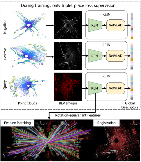
Figure 1: The overview of BEVPlace++. It projects point clouds into BEV images, and extracts rotation-equivariant local features and rotation-invariant global descriptors with our devised Rotation Equivariant and Invariant Network (REIN). It performs place recognition with global descriptors and then estimates poses using local features. BEVPlace++ only uses the triplet loss with positive and negative place samples for supervision, while achieving high performance in both place recognition and registration. The query BEV is colored red for better visualization.

I Introduction

Global localization aims to estimate the global poses of robots on a map without other prior information, which is a key component for achieving full autonomy of unmanned ground vehicles and crucial for many robotic applications. Especially in Simultaneous Localization and Mapping (SLAM) [1, 2, 3, 4], global localization provides loop closure constraints to eliminate accumulative drifts, essential for building globally consistent maps. Furthermore, it generates complementary pose estimations, which is important for initializing pose tracking or recovering it from failures [5, 6].

A widely adopted global localization paradigm typically first builds a global map with structure from motion or SLAM. When a query image or LiDAR scan is received, the system searches the map to find the best-matched place and then computes the global pose through sensor data registration. Over the past two decades, image-based global localization methods [7, 8, 2, 9, 10, 11] have been well-developed, thanks to the strong image features such as ORB [12] and SIFT [13]. Despite their broad usage in robotics, image-based methods are not robust enough to illumination changes and are sensitive to view changes due to the perspective imaging mechanism. In contrast, LiDARs actively emit infrared beams and measure the time of flight to perceive depth information, making LiDAR-based localization naturally robust to lighting changes [14]. Additionally, precise depth information provided by LiDARs allows for more accurate localization results. In the early days, LiDAR-based frameworks were less favored due to the immature manufacturing process of LiDARs. However, advancements in technology have made modern LiDARs more accurate, smaller, and cheaper, leading to their widespread application in fields such as mobile robots and autonomous driving. Thus, LiDAR-based global localization has become a hot topic and a crucial problem for robot perception tasks.

Despite the great potential of LiDAR in global localization, the sparsity of point clouds presents a significant challenge. Unlike image pixels organized in regular grids, point clouds are sparsely distributed in continuous 3D space, making it difficult to extract stable keypoints and distinctive features, which can lead to poor localization accuracy. Additionally, point clouds are typically dense for nearby scenes but sparse for distant ones, with varying sparsity across different types of LiDAR scanners. These factors complicate the generalization of LiDAR-based localization methods to different sensor configurations and new environments.

Some previous works tackle LiDAR localization by projecting point clouds into range images [15, 16, 17, 18]. Using range images avoids processing the sparse point clouds and shows promising performance across different environments. Moreover, the rotation of point clouds is equivalent to the horizontal shifting of range images, making range image-based methods robust to view rotations. However, range images suffer from scale distortions due to the spherical projection, limiting localization accuracy. Other methods try to use point networks to learn distinctive point features [19, 20, 21]. With accurate pose supervision, these approaches can achieve high localization accuracy but may not adapt well to different LiDAR scanner configurations or environments. Some methods build local maps from consecutive LiDAR scans and perform localization using these local maps [22, 23, 24]. While local maps can reduce the impact of sparsity, constructing them requires the robot to travel a certain distance and properly align the local map, which may compromise safety and is not always feasible.

This work introduces BEVPlace++, a fast, robust, and lightweight LiDAR global localization method for 3-DoF pose estimation without knowing the initial pose [25]. BEVPlace++ uses Bird’s Eye View (BEV) images as a simple yet effective and lightweight representation of LiDAR data. Unlike range images, BEV images provide more stable object scales and relationships, offering better generalization and easier deployment across different LiDAR sensors. By leveraging the translation equivariance of convolutional neural networks (CNNs) [26], we show that CNN features of BEV images are inherently distinctive and robust to the sparsity of LiDAR point clouds, allowing for accurate pose estimation between BEV image pairs. Such properties enable BEVPlace++ to generalize to unseen environments and adapt to different types of LiDAR scanners in a zero-shot learning manner. Additionally, we design a rotation equivariant Module (REM) to enhance BEVPlace++’s robustness to view changes. Both theoretical and statistical validations confirm the rotation equivariance of our devised REM, enabling BEV images with large view changes to be matched. Building based on REM, we propose a Rotation Equivariant and Invariant Network (REIN) by cascading REM with NetVLAD [27] to generate rotation equivariant local features and rotation invariant global descriptors. Unlike previous works requiring accurate pose labels [19, 28, 20, 21], BEVPlace++ achieves both place recognition and pose estimation using only coarse positive/negative place labels for supervision. An overview of the proposed method is depicted in Fig. 1. We use triplet supervision to minimize the feature distance of similar BEV images and maximize the distance of dissimilar ones. Benefiting from our designed translation and rotation equivariant network, such place supervision is sufficient to extract distinctive features on BEV images, allowing direct accurate pose estimation with Random Sample Consensus (RANSAC) [29] matching between BEV images.

In summary, the contributions of this work are five folds:

• We propose BEVPlace++, a complete global localization framework that utilizes the simple yet effective BEV representation of point clouds for both place recognition and pose estimation.

• We provide a detailed analysis of how the translation equivariance of CNN helps BEV image matching. Our BEVPlace++ accurately aligns BEV images with large translational differences using CNN features and effectively adapts to new, unseen environments.

• We propose a novel Rotation Equivariant and Invariant Network (REIN), constructed with lightweight CNN blocks and NetVLAD. It helps BEVPlace++ achieve robust place recognition and pose estimation under significant rotational view changes.

• We conducted comprehensive experiments on five different public datasets spanning various days, years, environments, and LiDAR scanner types. Our results demonstrate that BEVPlace++ achieves state-of-the-art performance across multiple tasks, including place recognition, loop closing, global localization, and SLAM.

• We open-source concise Python APIs of BEVPlace++, contributing to the robotics community.

BEVPlace++ is an extension of our previous conference paper BEVPlace [30]. BEVPlace uses group convolution to extract rotation equivariant local features from BEV images and achieves place recognition by global descriptor matching. Compared to BEVPlace, BEVPlace++ extends in four critical aspects: 1) a novel REIN network, with a faster and more light-weighted rotation equivariant and invariant feature encoder; 2) a deeper analysis of the rotation and translation equivariance of CNN features; 3) a complete pose estimator for achieving 3-DoF poses global localization; 4) more extensive and comprehensive experimental evaluations on various datasets, demonstrating superior performance in place recognition, loop closure detection, and complete global localization.

II Related Work

This section briefly overviews LiDAR-based global localization methods in the literature. Following existing surveys [31, 32], we categorize related works into three groups based on the integration degree of place recognition and pose estimation: 1) place recognition-only, that retrieves the most similar place using global descriptors; 2) global pose estimation, that directly estimates the global poses without retrieving places; and 3) place recognition followed by local pose estimation, that first achieves place recognition and then estimates the robot pose via a pose estimator.

1) Place recognition-only. These methods use a divide-and-conquer strategy, generating global descriptors for LiDAR scans and performing place recognition through descriptor retrieval. The pose of the retrieved place is then considered as the estimated pose. The key to place recognition is creating global descriptors that ensure similar scans are close in descriptor space while dissimilar ones are far apart. Early methods usually exploit the point statistics to represent the point cloud appearance. For example, M2DP [33] projects a point cloud to multiple 2D planes and generates a density signature for points in each plane. The singular value decomposition (SVD) components of the signature are then used to compute a global descriptor. Scan Context [34, 35] partitions the ground space into bins according to both azimuthal and radial directions and encodes the 2.5-D information within an image.

Recently, learning-based place recognition has been a hot topic, and many methods have been proposed. PointNetVLAD [14] leverages a network to project each point into a higher dimension feature and then uses NetVLAD [27] to generate global features. To take advantage of more contextual information, PCAN [36] introduces the point contextual attention network that learns attention to task-relevant features. Both PointNetVLAD and PCAN cannot capture local geometric structures due to the independent treatment for each point. Thus, the following methods focus on extracting more distinctive local features considering the neighborhood information. LPD-Net [37] adopts an adaptive local feature module to extract the handcrafted features and uses a graph-based neighborhood aggregation module to discover the spatial distribution of local features. EPC-Net [38] improves LPD-Net by using a proxy point convolutional neural network. SOE-Net [39] introduces a point orientation encoding (PointOE) module. Minkloc3D [40, 41] uses sparse 3D convolutions in local areas and achieves state-of-the-art performance on the benchmark dataset. Recently, some works including SVT-Net [42], TransLoc3D [43], NDT-Transformer [44], and PPT-Net [45] leverage the transformer-based attention mechanism [46] to boost place recognition performance. However, all these data-driven methods may lack generalization ability to unseen environments. Some methods explore the potential of the range image representation of point clouds. OverlapNet [15] uses the overlap of range images to determine whether two point clouds are at the same place and uses a Siamese network to estimate the overlap. OverlapTransformer [17] further uses a transformer architecture to learn rotation-invariant global features. CVTNet [18] combines range images and BEV images to perform matching. It transforms BEV images into a format similar to range images to achieve rotation-invariance. The range image-based methods usually have better generalization ability but suffer from the scale distortions of translation movements of point clouds.

2) Global pose estimation. These methods utilize the local characteristics of point clouds through geometric measures to generate local descriptors, which are then directly matched with a global map to determine the global poses. For example, the fast point feature histograms (FPFH) [47] uses the relationship between the neighbors of interest points and encodes them into a histogram. The Signature of Histograms of OrienTations (SHOT) [48] builds a local reference frame and leverages the orientation distribution of the normals in local regions. Although these methods can align local LiDAR scans, they usually lack descriptive capability in outdoor environments due to their sensitivity to point cloud density and noise. To leverage the local descriptors more efficiently, the keypoints voting method [49] performs localization using the 3D Gestalt descriptors. This method relies on robust keypoint extraction, while repeatable 3D keypoint detection is still an open problem in the literature. Some studies [50, 51] directly extract conventional image descriptors such as ORB [12] and SIFT [13] from LiDAR images for place recognition. These methods show promising performance in small environments but usually lack enough distinctiveness in large-scale outdoor environments. SegMatch [22] performs segmentation on LiDAR scans and builds a segment map. During online global localization, it extracts segments from the query LiDAR scan and matches them with the map. The following SegMap [23] further assigns the segment descriptors learned by a neural network to improve the matching performance. The main drawback of these methods is their reliance on traveling relatively long distances to extract distinctive segments by gathering multiple scans.

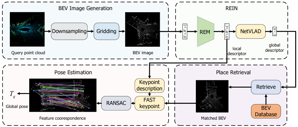
Figure 2: The pipeline of BEV image based global localization. Given a query point cloud, we generate its BEV image and sequentially extract local and global descriptors. The global descriptor is used for retrieving the most similar BEV from a pre-built database. The local descriptors are reused for pose estimation with RANSAC. The global pose of the query is computed as the combination of the pose of the match BEV and the relative pose.

3) Place recognition followed by local pose estimation. These approaches have been commonly used in visual global localization. However, it is not widely adopted in LiDAR global localization because few LiDAR local features have reached the same level of maturity as visual features like ORB and SIFT. To tackle the problem, BVMatch [52] projects point clouds into BEV images and extracts handcrafted BVFT features from the images. It then uses the bag-of-words model [7, 8, 11] to generate global features. However, it is shown that BVMatch cannot generalize well to unseen environments. BoW3D [53] extracts local features directly from sparse point clouds. It also adopts the bag-of-words model to generate global descriptors and is expected to show moderate generalization ability. Another line of work adopts deep learning techniques. For example, DH3D [19] uses the 3D local feature encoder and detector to extract local descriptors. It embeds the descriptors to a global feature for place recognition and aligns the matched LiDAR pairs using RANSAC [29]. The following methods such as LCDNet [20], LoGG3D-Net [28], and LCRNet [21] use a similar strategy and unify place recognition and pose estimation into one framework. LCDNet extracts distinctive local features with pointvoxel-RCNN [54] and performs data association with the Sinkhorn algorithm [55]. LoGG3D-Net [28] introduces a local consistency loss to guide the network toward learning local features consistently across revisits. LCRNet [21] exploits novel feature extraction and pose-aware attention mechanism to precisely estimate similarities and 6-DoF poses between pairs of LiDAR scans. By jointly learning local and global descriptors, these methods show satisfactory global localization performance. However, they may not adapt well when the point clouds are out of the distribution of the training data. BTC [24] extracts the keypoints of a point cloud by projecting the points to planes. It generates triangle descriptors and develops an efficient matching strategy. However, the BTC descriptor suffers from sparsity of point clouds as keypoints detection is unstable in sparse single LiDAR scans.

BEVPlace++ follows a two-step paradigm, sequentially performing place recognition and pose estimation for global localization. By first performing coarse localization through place recognition, unrelated scenes or BEV images can be effectively filtered out. In dynamic environments, the place recognition stage can help adapt to changes in the scene, such as lighting variations or partial occlusions. Unlike previous two-step-based methods, BEVPlace++ uses the BEV representation of point clouds. By leveraging the translation and rotation equivariance of CNNs, BEVPlace++ achieves robust pose estimation without requiring accurate pose supervision. Based on our devised REIN network, BEVPlace++ demonstrates remarkable generalization in unseen environments and adapts effectively to various sensor configurations.

III BEV-based Global Localization Pipeline

Our method uses bird’s eye view (BEV) images as an intermediate representation of LiDAR data to perform global localization. As shown in Fig. 2, we project point clouds into BEV views and extract distinct local and global descriptors with the rotation equivariant and invariant network (REIN). Then, we employ a two-stage localization paradigm, i.e., place recognition followed by pose estimation. In place recognition, we perform place retrieval with the global descriptors and find the top-matched BEV image from a pre-built database. In pose estimation, we exploit the local descriptors to estimate the relative pose between the query and matched BEV image pair using RANSAC. The global pose of the query is finally computed as the combination of the stored pose of the matched frame and the relative pose. In the following, we first explain the BEV image generation process, and then briefly describe the proposed REIN network. Finally, we elaborate on our proposed two-stage localization inference pipeline.

III-A Bird’s Eye View Representation

Following existing 3-DoF localization works [35, 16, 56], we assume that when the ground vehicle moves within a local area, it travels on a rough plane. Based on this assumption, we generate BEV images through the orthogonal projection and concentrate on estimating the pose in 3-DoF, including (x, y, yaw). The (z, pitch, roll) can also be derived from the stored pose of the matched frame, but they are not the primary focus of this article. The BEV image representation shows benefits in many aspects of our hierarchical localization system. In place recognition, BEV images offer a comprehensive view of the distribution of road elements. Therefore, it is more intuitive and stable to extract global descriptors from such images to depict the structural information of the scene. In the context of pose estimation, the transformations of BEV image pairs are estimated by solving the BEV image matching problem, which is fast because of the lightweight BEV representation. The lightweight BEV representation also benefits the storage resource which is important for real-world applications and multi-robot communication.

We use the normalized point density to construct BEV images [52]. Let $\mathcal{P}=\{P_{i}|i=1,...,N_{p}\}$ represent a point cloud formed by LiDAR points $P_{i}=(x_{i},y_{i},z_{i})$ with a total of $N_{p}$ points. We use the right-hand Cartesian coordinate system, where the x-axis points to the right, the y-axis points forward, the z-axis points upward, and the x-y plane is the ground plane. For a point cloud $\mathcal{P}$, we first use a voxel grid filter with the leaf size of $g$ meters to evenly distribute the points. Then we discretize the ground plane into grids with a resolution of $g$ meters. Considering a [$-D$ m $,D$ m] cubic window centered at the coordinate origin, BEV image $\textbf{I}(u,v)$ can be considered as a matrix of size $\lceil{\frac{2D}{g}}\rceil\times\lceil{\frac{2D}{g}}\rceil$. The BEV pixel value $\textbf{I}(u,v)$ is computed as the normalized point density with

$$\textbf{I}(u,v)=\frac{\min(N_{g},N_{m})}{N_{m}},$$ (1)

where $N_{g}$ denotes the number of points in the grid at position $(u,v)$ and $N_{m}$ the normalization factor. $N_{m}$ is set as the max value of the point cloud density.

Unlike traditional BEV image, also called elevation map [34, 35], that stores the maximum height of the points in each bin, we use the point densities. This is because the elevation map is sensitive to the orientation of the sensor, as the maximum height recorded varies with the distance between the scanner and the object. The density of points scanned on a surface, on the other hand, is less sensitive to viewpoint changes [52, 57].

III-B Rotation Equivariant and Invariant Netwrok

We propose a novel REIN network to extract local features of BEV images through devised rotation equivariant module (REM) and invariant global descriptors using NetVLAD [27]. Given a query BEV image $\textbf{I}_{q}\in\mathbb{R}^{H\times W}$, REM produces a feature map $\textbf{F}\in\mathbb{R}^{{H}^{\prime}\times{W}^{\prime}\times C}$, where $H^{\prime},W^{\prime},C$ is the height, width, and feature channels. Since the output feature map of REM is downsampled compared to the raw image size, we upsample the feature map with bilinear interpolation to assign descriptors for keypoints detected in the BEV image conveniently. These local descriptors are first aggregated by NetVLAD to generate a global descriptor $\textbf{V}\in\mathbb{R}^{K\times C}$ for place recognition where $K$ is the number of clusters in NetVLAD. The local descriptors are also reused in pose estimation. We will introduce the design of REIN in Sec. IV.

III-C Place Recognition

Place recognition assumes that point clouds close in feature space are also close geographically. We can retrieve a most apparently similar frame to a query BEV image $\textbf{I}_{q}$ from a pre-built BEV database according to the distances between global descriptors. The stored prior pose $\textbf{T}_{m}$ of the matched frame can be regarded as a coarse estimation of the query pose.

1) BEV Database construction. The BEV database contains necessary map information to achieve global localization, including keyframe BEV images, their associated global poses, and their descriptors. Suppose that the vehicle mounting a LiDAR sensor traverses a specific working area and collects LiDAR scans along the way. Every collected LiDAR scan in this traversal is tagged with a global pose by building a map using SLAM or GPS information. We generate a global descriptor for each collected LiDAR keyframe using our BEVPlace++ model. We denote the database formed by $n$ keyframes as a set

$$\mathcal{D}=\{(\mathbf{I}_{i},\mathbf{T}_{i},\mathbf{V}_{i})\}_{i=1,2,...,n}$$ (2)

where $\mathbf{T}_{i}\in\mathbb{R}^{3\times 3}$ and $\mathbf{V}_{i}\in\mathbb{R}^{K\times C}$ are the corresponding global pose and global descriptor of the BEV image $\mathbf{I}_{i}$. The database construction can be performed online or offline according to specific tasks. For localization within a global map, the database is typically constructed offline during the map-building process, far from the time of current application. For the task of loop closure in SLAM, the database is built in real-time, and its elements grow incrementally with the explored area of the vehicle.

2) Place retrieval. For the query BEV image $\textbf{I}_{q}$, we generate its global descriptor $\textbf{V}_{q}$ with BEVPlace++ feature extractor. The matched frame is computed through the nearest global descriptor searching:

$$m=\mathop{\arg}\limits_{i=1,2,...,n}\min||\mathbf{V}_{q}-\mathbf{V}_{i}||_{2}.$$ (3)

We regard the associated pose $\mathbf{T}_{m}$ as a rough estimation of the query pose $\mathbf{T}_{q}$. In practice, we use PCA to reduce all the global descriptors into 512-dim to speed up the reference.

III-D Pose Estimation

After finding the matched pair of BEV images, we match two BEV images by local descriptor matching and compute the BEV pose with RANSAC [29].

1) BEV image matching. We first extract FAST [58] keypoints from the BEV images to enable fast and accurate keypoint detection. Furthermore, on BEV images, the detected FAST keypoints usually have good repeatability since they are usually located at objects with vertical structures in the environment (e.g., poles, facades, guideposts). We then assign each keypoint with a local descriptor interpolated from the REM feature map. We perform local feature matching between the BEV image pair and use RANSAC to estimate the relative transform with the keypoint correspondences.

2) Global pose recovery. Since BEV images are generated from point clouds with orthogonal projection, the transform between BEV images is rigid. Once we know the transformation of BEV images, we can recover the transformation between the corresponding point clouds through a similar transformation. After obtaining the transform of $(\textbf{I}_{q}(u,v),\textbf{I}_{m}(u,v))$, we have:

$$\textbf{I}_{q}(u,v)=\textbf{I}_{m}(u^{\prime},v^{\prime})$$ (4)

$$u^{\prime}=\cos(\theta)u+\sin(\theta)v+t_{u}$$

$$v^{\prime}=-\sin(\theta)u+\cos(\theta)v+t_{v},$$

where $(t_{u},t_{v},\theta)$ are transform parameters. The transform matrix $\textbf{T}_{mq}$ of the corresponding scan+ pair ($\mathcal{P}_{m},\mathcal{P}_{q})$ is

$$\textbf{T}_{mq}=\begin{pmatrix}\cos(\theta)&\sin(\theta)&g{t_{u}}\\ -\sin(\theta)&\cos(\theta)&{g}{t_{v}}\\ 0&0&1\\ \end{pmatrix}$$ (5)

where $g$ is the BEV image resolution. As the global pose $\textbf{T}_{m}$ of the matched image is stored in the database, we could obtain the global pose of $\mathcal{P}_{q}$ as

$$\textbf{T}_{q}=\textbf{T}_{m}\textbf{T}_{mq}$$ (6)

IV Rotation Equivariant and Invariant Network

This section details the design of our rotation equivariant and invariant network (REIN), which includes a feature encoder for generating local features and a pooling layer for aggregating these local features into global descriptors. We begin by highlighting our finding that modern convolutional networks can effectively serve as distinctive feature encoders for BEV images under translation displacements. Then, we introduce a novel Rotation Equivariant Module (REM) to extract local features to achieve robustness to rotational view changes. Building on the rotation-equivariant local features, we show that our global descriptor, pooled by NetVLAD, is rotation-invariant. Finally, we elaborate on the network training strategy.

IV-A BEV Features Generation Through CNNs

Here, we provide a detailed statistical analysis of our finding that modern CNNs can serve as distinctive feature extractors for BEV images with translational movements. For clarity, we denote the process of feature extraction as

$$\textbf{F}=\phi(\textbf{I}),$$ (7)

where features $\textbf{F}\in\mathbb{R}^{H\times W\times C}$ are derived from a BEV image $\textbf{I}\in\mathbb{R}^{H\times W}$ through a feature extractor $\phi$. We denote the feature of a keypoint located at the coordinate $(u,v)$ as $\textbf{f}_{u,v}\in\mathbb{R}^{C}$, which also represents the element of F located at u-th row and v-th column with $C$ channels.

1) Distinctive BEV features from CNNs. We investigate the feature variation to validate the distinctiveness of BEV features from CNN extractors. For each keypoint feature $\textbf{f}_{u,v}$ extracted on our devised LiDAR BEV image, we compute its Eucleadian distance to its neighbor features by

$$d(\textbf{f}_{u,v},\textbf{f}_{u+\delta u,v+\delta v})=||\textbf{f}_{u,v}-\textbf{f}_{u+\delta u,v+\delta v}||_{2},$$ (8)

where $\delta u,\delta v$ are the translation displacements. Fig. 3 (a), (b), and (c) demonstrate an example of feature distance distribution for a specific feature extracted from a popular CNN, ResNet [26] with its pretrained model provided by PyTorch. We compute the feature distance of the keypoint feature shown in (a) relative to all other pixels and present the feature distance heatmap in (b). Additionally, (c) displays the numerical feature distance variation along the red scan line in (b). As can be seen, even without fine-tuning, the BEV feature distance increases as the translation displacement grows, indicating its inherent distinctiveness.

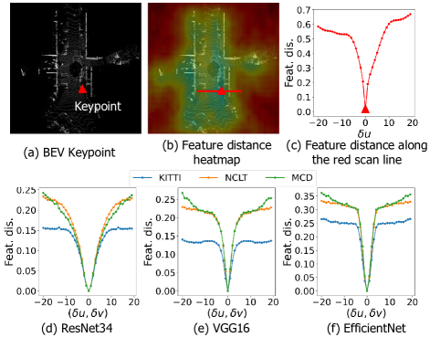
Figure 3: Statistical analysis: BEV feature distance distribution with respect to translation displacements with different CNN architectures and datasets. (a) A keypoint on a BEV image highlighted by a red triangle. (b) The feature distance heat map relative to all other pixels. (c) The feature distance variation along the red scan line in (b). (d) The average feature distance distribution concerning translation displacements (with $\delta u=\delta v$) using ResNet34 as the feature extractor. (e) The average feature distance distribution using VGG16. (f) The average feature distance distribution using EfficientNet.

We further plot the average feature distance with respect to translation displacements using different CNN backbones, including ResNet34 [26], VGG16 [59] and EfficientNet [60], on different datasets, such as KITTI [61], NCLT [62], and MCD [63], shown in Fig. 3 (e), (f), and (g). These datasets include point clouds collected by various types of LiDAR scanners with different fields of view and sparsity levels across diverse environments. As can be seen, spatially close features exhibit small feature distances while distant ones show larger feature distances, regardless of the dataset setup or used CNN backbones, which could formulated as

$$d(\textbf{f}_{u,v},\textbf{f}_{u+\delta u_{1},v+\delta v_{1}})<d(\textbf{f}_{u,v},\textbf{f}_{u+\delta u_{2},v+\delta v_{2}}),$$ (9)

$$for\quad||(\delta u_{1},\delta v_{1})||<||(\delta u_{2},\delta v_{2})||.$$

This inherent distinctiveness reveals that deep BEV features can capture and represent unique patterns in the BEV image. Such properties are crucial for accurately estimating pose, as they help in distinguishing between different keypoints and ensuring that their spatial relationships are preserved.

2) Matching with distinctive features. CNNs demonstrate translation equivariance [64] (up to edge-effects) due to local connectivity and weight sharing inherent in convolution operations. Given a BEV image $\textbf{I}^{\prime}$ obtained from I with translational motion, the keypoint feature $\textbf{f}^{\prime}_{u^{\prime},v^{\prime}}$ in $\textbf{I}^{\prime}$ should ideally be identical to its positional corresponding feature $\textbf{f}_{u,v}$ in I. Such correspondence should be unique according to Eq. 9, that is

$$d(\textbf{f}^{\prime}_{u^{\prime},v^{\prime}},\textbf{f}_{u,v})<d(\textbf{f}^{\prime}_{u^{\prime},v^{\prime}},\textbf{f}_{u+\delta u,v+\delta v}),$$ (10)

$$for\quad||(\delta u,\delta v)||>0.$$

Leveraging this characteristic, we establish BEV feature correspondences through nearest neighbor search and utilize RANSAC to solve for pose estimation. Because our matching approach does not rely on specific dataset fine-tuning, our method can effectively adapt to point clouds from various LiDAR scanners and generalize robustly across diverse environmental conditions.

Fig. 4 (a) illustrates feature matching results using ResNet34 under large translations. Each row corresponds to BEV images from the KITTI, NCLT, and MCD datasets, respectively. Following pose estimation, the overlaid BEV image pairs indicate our method’s capability to accurately estimate significant translation movements. It is noted that feature matching could fail under rotations, as shown in Fig. 4 (b), since CNNs are not rotation-equivariant and the feature distinctiveness is only preserved under translation transformations.

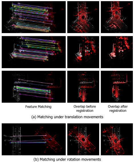
Figure 4: RANSAC matching utilizes BEV features extracted from a randomly initialized ResNet34. (a) Matching under translations. The three rows correspond to BEV images from the KITTI, NCLT, and MCD datasets, respectively. We illustrate the feature correspondences after RANSAC, BEV overlap before registration, and BEV overlap after registration from left to right. (b) Matching fails under rotations.

IV-B Rotation Equivariant Module

As discussed above, CNNs are translation equivariant but cannot handle rotations well. To achieve more robust pose estimations, we further design a network to extract rotation-equivariant feature maps from BEV images. We introduce a simple and effective rotation equivariant module (REM) to extract rotation equivariant local features. REM uses modern CNNs as basic modules to keep their representation ability to BEV images and achieves rotation equivariance by using the maximum CNN feature response of BEV images under different rotation transforms.

1) Rotation Equivariance Module Design. The architecture of REM is as illustrated in Fig. 5. Given an input BEV I, we warp it with the $N$ rotation angles from the angle set $\mathcal{R}=\{0,\frac{2\pi}{N_{R}},...,(N-1)\frac{2\pi}{N_{R}}\}$. For each rotated image, we extract local features with shared residual convolutional modules and rotate the feature map back. The equivariant local features are obtained by performing max pooling between $N$ rotated feature maps. The rotation equivariant features $F$ are obtained by

$$\textbf{F}=\max_{r\in\mathcal{R}}\textbf{R}^{-1}_{r}\circ{\phi(\textbf{R}_{r}\circ\textbf{I})}.$$ (11)

where $\phi$ is the residual convolutional modules.

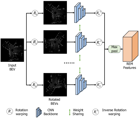
Figure 5: The architecture of rotation equivariant module (REM). Given an input BEV image, REM first warps the image with several rotation transforms. It then generates features for each warped image with weight-shared residual convolutional blocks. The output features are warped back with inverse rotations and are max pooled to obtain a rotation equivariant feature map.

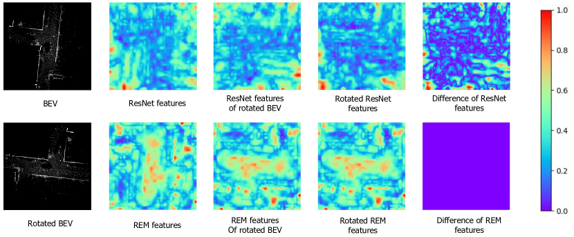
Figure 6: Comparison between ResNet features and REM features with rotations. Features are extracted from a pair of rotated BEV images with ResNet and REM, respectively. The difference between the ResNet features of the rotated BEV and the rotated ResNet features of the original BEV is large. On the other hand, REM shows rotation equivariance, and the difference between the REM features of the rotated BEV and the rotated REM features of the original BEV tends to be zero.

2) Rotation Equivariance Analysis. Applying a rotation $\textbf{R}_{\alpha}\in\mathcal{R}$ to the BEV image I, the output feature map $\textbf{F}^{\prime}$ is

$$\textbf{F}^{\prime} =\max_{r\in\mathcal{R}}\textbf{R}^{-1}_{r}\circ{\phi((\textbf{R}_{r}\textbf{R}_{\alpha})\circ\textbf{I})}.$$ (12)

We apply an identical transformation $\textbf{R}_{\alpha}\textbf{R}^{-1}_{\alpha}$ to the feature map and have

$$\textbf{F}^{\prime} =\max_{r\in\mathcal{R}}\textbf{R}_{\alpha}\textbf{R}_{\alpha}^{-1}\textbf{R}^{-1}_{r}\circ{\phi((\textbf{R}_{r}\textbf{R}_{\alpha})\circ\textbf{I})}$$ (13)

$$=\textbf{R}_{\alpha}\circ\max_{r\in\mathcal{R}}\textbf{R}_{\alpha}^{-1}\textbf{R}^{-1}_{r}\circ{\phi((\textbf{R}_{r}\textbf{R}_{\alpha})\circ\textbf{I})}.$$

$$=\textbf{R}_{\alpha}\circ\max_{r\in\mathcal{R}}\textbf{R}_{r+\alpha}^{-1}\circ{\phi((\textbf{R}_{r+\alpha})\circ\textbf{I})}$$

$$=\textbf{R}_{\alpha}\circ\textbf{F}.$$

This validates the REM feature map $\textbf{F}^{\prime}$ of the rotated image is equal to the rotated feature map $\textbf{F}_{\alpha}$ of the raw BEV image. Theoretically, we need to sample infinite angles to achieve continuous rotation equivariance. In our experiments, we find a small $N$ can achieve satisfactory performance. This is possible because the pooling and downsample operations in CNN could provide some robustness to small movements.

Fig. 6 illustrates the comparison between ResNet and REM features under rotations. We extract features from a pair of rotated BEV images with ResNet and REM, respectively. As can be seen, the difference between the REM features of the rotated BEV and the rotated REM features of the original BEV tends to be zero, showing the rotation equivariance of REM. On the other hand, ResNet does not own such equivariance and its feature map difference with rotational changes is large.

3) Discussion. We have demonstrated that modern CNN networks are highly effective for extracting distinctive features from our devised BEV images. Leveraging the strengths of CNN modules, our REM network preserves this distinctiveness while further addressing BEV image matching under significant translational and rotational changes. Consequently, BEVPlace++ does not require accurate pose supervision, making it convenient for real-world deployment, where obtaining accurate pose information is often challenging.

IV-C Rotation Invariant Global Descriptor.

For robust place recognition, we design a network $\beta$ to extract rotation-equivariant features from BEV images such that any rotation transformation on the input image will result in the same global descriptors, which can be formulated as

$$\beta(\textbf{R}\circ\textbf{I})=\beta(\textbf{I}).$$ (14)

We use the cascading of REM and NetVLAD to generate such rotation-invariant global descriptors.

1) NetVLAD. NetVLAD [27] is a widely used method for pooling descriptors in image retrieval. It assumes similar structures in the environment produce similar distributions of features and summarizes information about the distributions across an image into a global descriptor. We first constructs K cluster centers denoted as $\{\mathbf{c}_{i}|\mathbf{c}_{i}\in\mathbb{R}^{C}\}_{i=1,...,K}$. Denoting $\{\textbf{f}_{i}|\textbf{f}_{i}\in\mathbb{R}^{C}\}_{i=1,...,{H^{\prime}W^{\prime}}}$ be the set of local features flattened from the REM feature map F, we generate a global feature $\mathbf{V}=[\mathbf{V}_{1},\mathbf{V}_{2},...,\mathbf{V}_{K}]$ of dimension $C\texttimes K$. $\textbf{V}_{k}$ is the weighted sum of residuals of all local features with respect to the k-th cluster center, namely

$$\mathbf{V}_{k}=\sum_{i}v_{k}(\mathbf{f}_{i})=\sum_{i}\frac{e^{\mathbf{w}_{k}^{T}\mathbf{f}_{i}+b_{k}}}{\sum_{k^{\prime}}e^{{\mathbf{w}_{k^{\prime}}^{T}\mathbf{f}_{i}+b_{k^{\prime}}}}}(\mathbf{f}_{i}-\mathbf{c}_{k}),$$ (15)

where $\mathbf{w}_{k}$ and $b_{k}$ are the learnable weights and bias.

2) Rotation Invariance Analysis. Let $\{\mathbf{f}_{i}\}_{i=1,...,{H^{\prime}W^{\prime}}}$ and $\{\mathbf{f^{\prime}}_{i}\}_{i=1,...,{H^{\prime}W^{\prime}}}$ be the local descriptor sets of the raw BEV image and the rotated image. As the REM feature map is rotation equivariant, set $\{\mathbf{f}_{i}\}_{i=1,...,H^{\prime}W^{\prime}}$ and $\{\mathbf{f^{\prime}}_{i}\}_{i=1,...,H^{\prime}W^{\prime}}$ has same elements but different permutation. We have

$$\mathbf{V}_{k}^{\prime} =v_{k}(\mathbf{f}_{1}^{\prime})+v_{k}(\mathbf{f}_{2}^{\prime})+...+v_{k}(\mathbf{f}_{n}^{\prime})$$ (16)

$$=\sum_{i}v_{k}(\mathbf{f}_{i}^{\prime})$$

$$=\sum_{i}v_{k}(\mathbf{f}_{i})=\mathbf{V}_{k},$$

indicating the rotation invariance of global descriptors.

TABLE I: Evaluation Datasets.

Dataset	KITTI [61]	NCLT  [62]	MCD [63]	RobotCar [65]	Inhouse [14]
LiDAR	Velodyne HDL-64E	Velodyne HDL-32E	Livox Mid-70	SICK LD-MRS 3D	Velodyne HDL-64
Field of View (HxV)	360.0${}^{\circ}\times$ 26.8∘	360.0${}^{\circ}\times$ 41.3∘	70${}^{\circ}\times$ 70 ∘ (non repeat)	85.0${}^{\circ}\times$ 3.2∘	360.0${}^{\circ}\times$ 26.8∘
No. of Sequences	5	7	6	44	15
Scenes	City, Country	Campus	City	City	Campus
Cities	Karlsruhe	Michigan	Singapore	Oxford	Singapore
Trajectory length	5 km	10 km	2km	10 km	10 km
Time span	Single days	Across 1 year	Single days	Across 1 year	Several days
Evaluation	PR & LC & GL	PR & LC	PR & GL	PR	PR

• PR, LC, and GL correspond to place recognition, loop closure, and global localization.

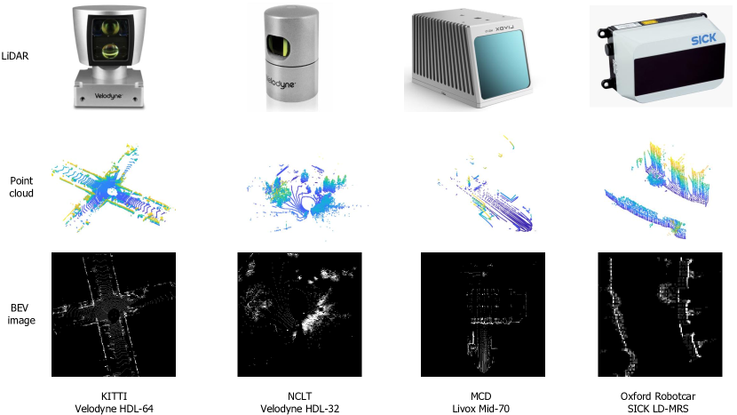
Figure 7: Sample data of different datasets, including the first-row LiDAR scanners, the second-row point clouds, and the third-row corresponding BEV images.

IV-D Network Training

1) Loss function. We aim to train the BEVPlace++ network such that the geographically close BEV images are close in the feature space, and geographically distant BEV images are far apart. We use the lazy triplet loss [14] to supervise the global descriptor generation. The lazy triplet loss focuses on maximizing the feature distance between a query and its closest/hardest negative sample in the training set, that is

$$\mathcal{L}=\max_{j}\bigl{(}\max(m+||\textbf{V}_{a}-\textbf{V}_{p}||_{2}-||\textbf{V}_{a}-\textbf{V}_{nj}||_{2},0)\bigr{)},$$ (17)

where $\textbf{V}_{p},\textbf{V}_{nj}$ are the global descriptors of the positive and j-th negative sample of the query, $\textbf{V}_{p}$ is the global descriptor of the query BEV image, and $m$ is the constant margin. In our design, we do not supervise the REM network since the deep BEV features from REM are inherently distinctive as discussed before.

2) Training setups. We assume that the ground vehicle mounting a LiDAR sensor traverses a specific working area and collects LiDAR scans along the way. Every LiDAR scan collected in this traversal is tagged with a global pose from a SLAM method or GPS information. Note that, these global poses are not necessarily to be very accurate, as we only need them to determine the positive and negative samples with a rough distance threshold. We use every collected scan tagged with a global pose as a query frame. For each query frame, its positive samples are the ones within $5$ meters away from itself and its negative samples are the other frames. Then, the training process is to traverse all the queries and perform gradient descent under the supervision of Eq. 17. We also adopt the hard mining strategy [66] following NetVLAD after the first 10 training epochs.

V Evaluation Setup

V-A Datasets

We selected datasets to thoroughly evaluate the performance of our method in large-scale environments, under long-term changes, and with various LiDAR sensor setups. The evaluation datasets include KITTI [61], NCLT [62], MCD [63], the RobotCar [65], and In-house dataset [14], which were collected in different cities.

We evaluate loop closing performance on KITTI and NCLT datasets since their data sequences have large loops. We test global localization on KITTI, NCLT, and MCD datasets as they have accurate ground truth poses. We evaluate place recognition on all the datasets. Our evaluation datasets cover diverse scenes, including city, countryside, and campus, and are collected in large-scale places under large time spans. The point cloud data are of different sparsity and different fields of view due to the usage of the various types of LiDAR sensors. Tab. I summarizes the meta information of the datasets. Fig. 7 provides some example point clouds and their corresponding BEV images. As can be seen, the point clouds in these datasets differ greatly, presenting sufficient challenges for evaluating reliable single-shot global localization. We detailed our setups of each dataset as follows:

1) KITTI [61]. This dataset contains a large number of point cloud data collected by a Velodyne 64-beam LiDAR. We select the sequences “00”, “02”, “05”, “06”, “07”, and “08” of the Odometry subset for evaluation since these sequences contain large revisited areas. We split the point clouds of each sequence into database frames and query frames for place retrieval. The partition of each sequence is summarized in Tab. II. We use the refined ground truth poses from semantic KITTI [67] with a distance threshold to determine if a loop closure exists.

TABLE II: Dataset Partition of the KITTI dataset.

Seq.	00	02	05	06	08
Db.	0-3000	0-3400	0-1000	0-600	0-3000
Query	3200-4650	3600-4661	1200-2751	800-1100	3200-4645

2) NCLT [62]. This dataset was created at the University of Michigan North Campus using a Velodyne32-HDL LiDAR sensor. The dataset provides ground-truth poses based on a large SLAM solution using LiDAR scan matching and high-accuracy RTK-GPS. The sequences of the dataset are collected on varying routes and cover different parts of the campus across a year. We select sequences collected in different seasons for evaluation, including “2012-01-15”, “2012-02-04” “2012-03-17”, “2012-06-15”, “2012-09-28”, “2012-11-16”, and “2013-02-23” .

3) MCD [63]. This dataset is collected over large-scale campus areas at different seasons. We use its point cloud data from a non-repetitive lidar, Livox MID-30. The clouds have a circular field of view and are quite different from the clouds of rotating-beam LiDAR. For evaluation, we use the sequences collected at NTU including “ntu_day_01”, “ntu_day_02”, “ntu_day_10”, “ntu_night_04”, “ntu_night_08”, “ntu_night_13”.

4) RobotCar [65] and In-house [14]. These two datasets are broadly used by the recent place recognition method based on unordered points. The RobotCar dataset was created with a SICK LD-MRS LiDAR by repeatedly visiting a route of 10 km in Oxford. It contains 44 sequences collected on different days across a year. The In-house dataset consists of three scenarios including a university sector (U.S.), a residential area (R.A.), and a business district (B.D.). It is constructed from Velodyne-64 LiDAR scans and each of them contains have 5 sequences. Different from the aforementioned datasets that provide single LiDAR scans, these two datasets provide submaps built from consecutive scans.

V-B Evaluation Metrics

We use different metrics to evaluate different tasks. For place recognition, we use the recall rate at top-1 following previous works [30, 68, 14]. For each query, we find its Top-1 match from the database. According to a distance threshold of 5 meters [30], we determine whether the prediction is a true positive (TP), a false negative (FN), or a false positive (FP). The recall rate is defined as the ratio of TP over the actual positives, i.e.

$$\text{Recall}=\frac{\text{TP}}{\text{TP}+\text{FN}}.$$ (18)

For loop closing with loop closure detection and pose estimation, we use the Precision-Recall (PR) curve, average precision, F1 max score, max recall at 100% precision, mean translation errors, and mean rotation errors. The PR curve relies on both recall rates and precision, where precision is computed as the ratio of true positives (TP) over all predicted positives, i.e.

$$\text{Precision}=\frac{\text{TP}}{\text{TP}+\text{FP}}.$$ (19)

Similar to the evaluation of place recognition, we compute the nearest descriptor distance for a query and retrieve the top-1 match from the database. By setting different descriptor distance thresholds, we calculate the corresponding precision and recall pair and plot a PR curve. The average precision is the area under the PR curve. The F1 score is

$$\text{F1 score}=2\times\frac{\text{Precision}\times\text{Recall}}{\text{Precision}+\text{Recall}}.$$ (20)

We obtain the max recall at 100% precision by traversing all the precision and recall pairs. The mean rotation and translation errors are computed with the pose errors of all the true positive queries.

For complete global localization, we evaluate mean translation errors and mean rotation errors. Following [21], we also compute the localization success rate (SR) under a threshold of $(2m,5^{\circ})$.

TABLE III: Recall at Top-1 on the KITTI dataset.

Sequence	00	02	05	06	08	Mean
M2DP [34]	92.9	69.3	80.7	94.8	34.4	74.4
Logg3D[28]	99.6	96.1	97.5	100.0	93.5	97.3
CVTNet [39]	98.7	87.1	93.5	97.8	83.7	92.1
BoW3D [37]	71.4	15.5	58.7	91.8	57.0	58.9
LCDNet [40]	99.9	97.7	95.3	100.0	94.4	97.4
BEVPlace [30]	99.7	98.1	99.3	100.0	92.0	97.8
BEVPlace++ (ours)	100.0	99.3	100.0	100.0	99.1	99.7

TABLE IV: Recall at Top-1 on the rotated KITTI dataset.

Sequence	00	02	05	06	08	Mean
M2DP [34]	92.9	69.3	80.7	94.8	34.4	74.4
BoW3D [37]	19.2	9.1	13.5	13.4	1.5	11.3
Logg3D[28]	99.4	96.4	97.3	99.6	92.0	96.9
CVTNet [39]	98.7	87.4	93.3	98.5	85.8	92.7
LCDNet [40]	99.7	98.1	95.5	100.0	94.7	97.6
BEVPlace [30]	99.6	93.5	98.9	100.0	92.0	96.8
BEVPlace++ (ours)	99.7	97.1	98.9	100.0	97.3	98.6

VI Experiments

In this section, we conduct experiments to evaluate the performance of our method in terms of place recognition, loop closing, and complete global localization. We compare our method with state-of-the-art methods including M2DP [33], CVTNet [18], Logg3D-Net [28], BoW3d [53], and LCDNet [20]. Among these methods, BoW3d and LCDNet can estimate poses, while the other 3 methods can only perform place recognition and loop closure detection.

TABLE V: Generalization Performance of Recall at Top-1 on NCLT and MCD datasets.

	NCLT						MCD_ntu
	2012-02-04	2012-03-17	2012-06-15	2012-09-28	2012-11-16	2013-02-23	day_02	day_010	night_04	night_08	night_13
M2DP [33]	63.2	58.0	42.4	40.6	49.3	27.9	46.7	65.5	56.1	55.7	59.8
BoW3D [53]	14.9	10.7	6.5	5.0	5.2	7.5	0.0	0.0	0.0	0.0	0.0
CVTNet [18]	89.2	88.0	81.2	74.9	77.1	80.3	80.0	84.8	82.0	83.9	85.9
LoggNet [28]	69.9	19.6	11.0	8.7	10.9	25.6	6.9	12.7	8.8	10.9	10.4
LCDNet [20]	60.5	54.2	44.2	34.9	31.7	10.9	45.6	53.5	50.3	46.2	48.9
BEVPlace [30]	93.5	92.7	87.4	87.8	88.9	86.2	79.1	87.4	80.5	85.9	83.7
BEVPlace++	95.3	94.2	90.2	88.9	91.3	87.8	83.1	90.2	86.6	88.9	86.4

TABLE VI: Recall rates on the benchmark dataset.

	Oxford		U.S.		R.A.		B.D		Mean
	AR@1	AR@1%	AR@1	AR@1%	AR@1	AR@1%	AR@1	AR@1%	AR@1	AR@1%
PointNetVLAD [14]	62.8	80.3	63.2	72.6	56.1	60.3	57.2	65.3	59.8	69.6
LPD-Net [37]	86.3	94.9	87.0	96.0	83.1	90.5	82.5	89.1	84.7	92.6
NDT-Transformer [44]	93.8	97.7	-	-	-	-	-	-	-	-
PPT-Net [45]	93.5	98.1	90.1	97.5	84.1	93.3	84.6	90.0	88.1	94.7
SVT-Net [42]	93.7	97.8	90.1	96.5	84.3	92.7	85.5	90.7	88.4	94.4
TransLoc3D [43]	95.0	98.5	-	-	-	-	-	-	-	-
MinkLoc3Dv2 [41]	96.3	98.9	90.9	96.7	86.5	93.8	86.3	91.2	90.0	95.1
BEVPlace	96.5	99.0	96.9	99.7	92.3	98.7	95.3	99.5	95.3	99.2
BEVPlace++ (ours)	96.2	99.1	97.1	99.7	92.7	98.8	95.6	99.6	95.4	99.3

Implementation details. For all baseline methods, we reproduce their results using their open-source implementations with default setups. For BEVPlace++, we use ResNet34 as the backbone in REM. The ResNet is cropped to retain the first three layers (up to conv3_x), resulting in an output channel number $C$ of 128. The number of rotations $N_{R}$ in REM is empirically set to 8. The point cloud crop range $D$ is set to 40 meters, and the grid size $g$ for BEV image generation is 0.4 meters. Consequently, the BEV image has a size of $200\times 200$. We train BEVPlace++ with the AdamW optimizer for 50 epochs. The learning rate is initially set as 1e-4 and decays by a factor of 2 every 10 epochs. The weight decay is set to 1e-3. The method is trained on an RTX 3090 GPU.

VI-A Place Recognition

We conduct experiments to fully evaluate the performance of place recognition including the robustness to view changes, generalization ability, and long-term stability.

Performance on KITTI. We only train the methods on KITTI dataset using the database of sequence “00”, which contains 3000 frames. We apply data augmentation by randomly rotating the point clouds to improve the robustness to view changes. As can be seen in Tab. III, our BEVPlace++ outperforms M2DP, Scan Context, BoW3D, and CVTNet with large margins. Logg3d-Net and LCDNet achieve comparable performance to BEVPlace++. However, they perform much worse than BEVPlace++ on the challenging sequence “08” which has a large amount of challenging reverse loops.

Robustness to view changes. To test the robustness against rotational changes, we randomly rotate all the query and database point clouds around the z-axis with an angle range of $[0,2\pi)$ to simulate view changes. As shown in Tab. IV, our BEVPlace++ maintains the highest recall rates, benefiting from our rotational invariant global descriptor designs. CVTNet, Logg3d-Net, and LCDNet are also robust to rotations to some extent. However, BoW3D’s performance significantly degenerated compared to those without rotation changes.

Generalization ability and Long-term performance. We evaluate the methods on NCLT and MCD datasets using models trained on KITTI. For NCLT, we construct the database with the sequence “2012-01-15” that covers most areas of the campus. We then perform place retrieval using the point clouds of other sequences, including the one collected in 2013 across a year. For MCD, we build the database with the sequence “ntu_day_01” and perform place retrieval using other sequences, including the three night sequences. These two datasets are collected using different types of LiDAR scanners compared to that used in KITTI and their point clouds are sparser. Tab. V shows the recall rates at Top-1 on the two datasets. As can be seen, BEVPlace++ achieves high recalls on NCLT regardless of season changes. The compared methods rather have much lower recall rates. BEVPlace++ consistently outperforms other methods on MCD with day-night changes.

TABLE VII: Average precision and F1 max score of loop closure on KITTI and NCLT.

Sequence	KITTI 00					KITTI 02					KITTI 05					KITTI 06
	AP	max F1	max Recall (%)	$\hat{e}_{t}$ (m)	$\hat{e}_{r}$ $(^{\circ})$	AP	max F1	max Recall (%)	$\hat{e}_{t}$ (m)	$\hat{e}_{r}$ $(^{\circ})$	AP	max F1	max Recall (%)	$\hat{e}_{t}$ (m)	$\hat{e}_{r}$ $(^{\circ})$	AP	max F1	max Recall (%)	$\hat{e}_{t}$ (m)	$\hat{e}_{r}$ $(^{\circ})$
M2DP [34]	0.982	0.936	86.7	-	-	0.884	0.844	0.0	-	-	0.946	0.897	68.1	-	-	0.974	0.938	76.2	-	-
Logg3D[28]	0.995	0.976	55.2	-	-	0.983	0.927	82.7	-	-	0.995	0.975	86.2	-	-	0.996	0.970	91.9	-	-
CVTNet [39]	0.994	0.965	84.8	-	-	0.931	0.898	64.6	-	-	0.975	0.933	96.2	-	-	0.996	0.981	96.2	-	-
BoW3D [37]	0.979	0.897	46.5	0.54	1.20	0.559	0.546	10.6	0.74	0.55	0.957	0.857	47.8	0.69	0.72	0.992	0.968	48.1	0.62	0.73
LCDNet [40]	0.997	0.974	94.1	0.10	0.14	0.976	0.928	83.7	0.65	0.44	0.994	0.964	93.0	0.12	0.17	0.999	0.997	99.6	0.11	0.17
BEVPlace++	0.999	0.995	98.4	0.08	0.11	0.977	0.934	70.0	0.38	0.70	0.994	0.982	96.2	0.12	0.09	0.999	0.999	100.0	0.18	0.08
	KITTI 08					NCLT 2012-01-15					NCLT 2012-02-04					NCLT 2012-03-17
	AP	max F1	max Recall (%)	$\hat{e}_{t}$ (m)	$\hat{e}_{r}$ $(^{\circ})$	AP	max F1	max Recall (%)	$\hat{e}_{t}$ (m)	$\hat{e}_{r}$ $(^{\circ})$	AP	max F1	max Recall (%)	$\hat{e}_{t}$ (m)	$\hat{e}_{r}$ $(^{\circ})$	AP	max F1	max Recall (%)	$\hat{e}_{t}$ (m)	$\hat{e}_{r}$ $(^{\circ})$
M2DP [34]	0.081	0.162	0.0	-	-	0.783	0.695	4.8	-	-	0.700	0.620	3.7	-	-	0.654	0.621	4.0	-	-
Logg3D[28]	0.958	0.929	2.7	-	-	0.679	0.592	1.0	-	-	0.575	0.517	0.6	-	-	0.570	0.530	1.4	-
CVTNet [39]	0.848	0.721	26.0	-	-	0.947	0.876	20.5	-	-	0.923	0.863	30.3	-	-	0.907	0.836	11.2	-	-
BoW3D [37]	0.905	0.829	14.4	1.44	2.81	0.000	0.000	0.0	-	-	0.000	0.000	0.0	-	-	0.000	0.000	0.0	-	-
LCDNet [40]	95.2	91.8	12.2	0.21	0.47	0.633	0.342	0.0	0.39	1.20	0.621	0.362	0.0	0.37	1.16	0.684	0.321	0.0	0.37	1.26
BEVPlace++	0.999	0.984	76.4	0.35	0.57	0.963	0.912	24.9	0.34	1.09	0.969	0.916	34.5	0.36	1.19	0.935	0.859	31.2	0.40	1.17
	NCLT 2012-06-15					NCLT 2012-09-28					NCLT 2012-11-16					NCLT 2013-02-23
	AP	max F1	max Recall (%)	$\hat{e}_{t}$ (m)	$\hat{e}_{r}$ $(^{\circ})$	AP	max F1	max Recall (%)	$\hat{e}_{t}$ (m)	$\hat{e}_{r}$ $(^{\circ})$	AP	max F1	max Recall (%)	$\hat{e}_{t}$ (m)	$\hat{e}_{r}$ $(^{\circ})$	AP	max F1	max Recall (%)	$\hat{e}_{t}$ (m)	$\hat{e}_{r}$ $(^{\circ})$
	AP	max F1	$\hat{e}_{t}$	$\hat{e}_{r}$	AP	max F1	$\hat{e}_{t}$	$\hat{e}_{r}$	AP	max F1	$\hat{e}_{t}$	$\hat{e}_{r}$	AP	max F1	$\hat{e}_{t}$	$\hat{e}_{r}$
M2DP [34]	0.666	0.617	1.9	-	-	0.676	0.602	4.2	-	-	0.281	0.380	0.0	-	-	0.700	0.656	1.3	-	-
Logg3D[28]	0.427	0.413	0.3	-	-	0.509	0.476	1.0	-	-	0.282	0.279	0.0	-	-	0.511	0.472	0.2	-	-
CVTNet [39]	0.937	0.869	36.8	-	-	0.920	0.840	19.7	-	-	0.784	0.719	8.1	-	-	0.897	0.823	15.4	-	-
BoW3D [37]	0.024	0.102	0.0	-	-	0.000	0.000	0.0	-	-	0.000	0.000	0.0	-	-	0.000	0.000	0.0	-	-
LCDNet [40]	0.628	0.288	0	0.50	1.30	0.552	0.244	0.0	0.44	1.27	0.243	0.039	0.0	0.47	1.55	0.231	0.191	0.0	0.52	1.68
BEVPlace++	0.955	0.901	63.4	0.40	1.19	0.957	0.894	45.3	0.40	1.61	0.839	0.733	15.8	0.40	1.10	0.959	0.887	45.5	0.44	1.05

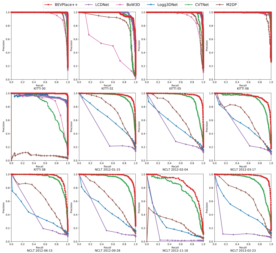
Figure 8: PR curve performance of different methods on KITTI and NCLT datasets.

Performance on sparse point maps of the RobotCar and Inhouse dataset. The two datasets provide point clouds downsampled to 4096 points and normalized to range $[-1,1]$. They contain coarse position ground truth. While the compared methods need raw points input or accurate pose supervision, we do not evaluate them on this dataset. Instead, we compare our method with the methods consuming normalized points, including NDT-Transformer [44], PPT-Net [45], SVT-Net [42], and TransLoc3D [43]. For our method, we generate BEV images of size 200$\times$200. Following the previous works [14, 37], we train our method only with the RobotCar training dataset and test the method on the test set. For all the compared methods, we directly use the results from their papers. Tab. VI shows that our BEVPlace++ outperforms other methods including the transformer-based ones with large margins. In particular, our method generalizes well to U.S, R.A, and B.D subsets, while other methods have relatively large performance degradation.

VI-B Loop Closing

Similar to the setup in place recognition, we test the methods with models trained on sequence “00” of KITTI. We perform evaluation on every single sequence. For each frame in a sequence, we perform place retrieval in the former frames with the nearest 100 frames excluded.

Tab. VII presents a quantitative comparison of average precision, F1 max score, max recall at 100% precision, mean translation errors, and mean rotation errors. BEVPlace++ achieves an average precision over 90% on both datasets. While LCDNet and Logg3DNet also show high precision on KITTI, their precision and F1 max scores are significantly lower on NCLT. Conversely, BoW3D fails to generalize to NCLT. Notably, BEVPlace++ achieves a significantly higher maximum recall at 100% precision on sequence ”08” compared to other methods. This high level of precision is crucial because false positive detections can introduce irreversible errors into downstream tasks such as loop correction and map updating. Ensuring a high recall at perfect precision means that BEVPlace++ can reliably recognize places without mistakenly identifying incorrect matches, thus maintaining the integrity and accuracy of subsequent processing steps in autonomous navigation systems. Additionally, BEVPlace++ demonstrates low mean translation and rotation errors on both datasets, specifically below 0.5 meters and 1.5 degrees, respectively. These small errors are significant because they indicate a high level of initial accuracy in the localization process. The full PR curves are illustrated in Fig. 8. As shown, BEVPlace++ outperforms all baseline methods in terms of PR curve evaluation. Especially on NCLT, BEVPlace++ has a much higher curve.

TABLE VIII: Complete Global Localization Performance on different datasets.

Dataset	Sequence	BoW3D				LCDNet				BEVPlace++
		Recall (%) $\uparrow$	SR(%) $\uparrow$	$\bar{e}_{t}$ (m) $\downarrow$	$\bar{e}_{r}$ (∘) $\downarrow$	Recall (%) $\uparrow$	SR(%) $\uparrow$	$\bar{e}_{t}$ (m) $\downarrow$	$\bar{e}_{r}$ (∘) $\downarrow$	Recall (%) $\uparrow$	SR(%) $\uparrow$	$\bar{e}_{t}$ (m) $\downarrow$	$\bar{e}_{r}$ (∘) $\downarrow$
NCLT	2012-02-04	14.9	3.8	1.11	2.08	60.5	58.5	0.37	1.15	95.3	95.6	0.32	1.06
	2012-03-17	10.7	3.0	1.02	2.44	54.2	52.0	0.37	1.26	94.2	95.1	0.33	1.18
	2012-06-15	6.5	1.1	1.23	2.62	44.2	40.0	0.49	1.28	90.2	90.9	0.42	1.11
	2012-09-28	5.0	0.6	0.92	1.98	34.9	32.2	0.44	1.27	88.9	89.8	0.46	1.23
	2012-11-16	5.2	0.3	1.27	2.36	31.7	28.8	0.47	1.54	91.3	90.2	0.44	1.65
	2013-02-23	7.5	1.1	1.05	2.14	10.9	6.8	0.50	1.62	87.8	88.5	0.37	1.05
MCD ntu	day_02	0.0	0.0	-	-	45.6	29.9	1.06	0.91	83.1	77.9	0.75	1.08
	day_10	0.0	0.0	-	-	53.5	37.3	0.88	0.90	90.2	88.8	0.61	1.03
	night_04	0.0	0.0	-	-	50.3	30.3	1.01	0.98	86.6	80.9	0.62	1.01
	night_08	0.0	0.0	-	-	46.2	33.7	0.89	0.94	88.9	85.7	0.64	1.08
	night_13	0.0	0.0	-	-	48.9	36.1	0.92	0.99	86.4	85.9	0.72	1.21

VI-C Complete Global Localization

Here, we conduct experiments to evaluate the accuracy of complete global localization, which estimates 3-DoF poses against a pre-built map without knowing the initial pose. For each query, we retrieve its Top-1 match from the database via place recognition and then compute the global pose using pose estimation. Tab. VIII shows the recall of place retrieval, localization success rates, mean translation error, and mean rotation error. Our BEVPlace++ generalizes better on NCLT and MCD compared to LCDNet and BoW3D, demonstrating its superiority across different sensor configurations and diverse environments. Notably, the localization success rate of BEVPlace++ on NCLT may be higher than the retrieval recall rate. This occurs when BEVPlace++ successfully estimates the pose of a query even when the distance between the query and the Top-1 match is larger than 5 meters. It should be noted that BEVPlace++ does not use pose supervision, making it much easier for deployments than methods like LCDNet [20].

VI-D Runtime Analysis

We compare the runtime of the methods on a desktop equipped with an RTX 3090 GPU and an Intel quad-core 3.40 GHz i5-7500 CPU. Tab. IX shows the running time of each stage on the KITTI dataset. Our BEVPlace++ comprises simple residual and NetVLAD blocks, enabling it to run fast and achieve an average frequency of over 40 Hz for place recognition. For complete global localization, it takes about 41.6 ms for pairwise feature extraction, 0.24 ms for place retrieval, and 12.7 ms for pose estimation, achieving an average frequency of over 20 Hz. Considering that the frequency of LiDAR scans is usually set to 10 Hz, BEVPlace++ can operate in real time.

TABLE IX: Recall at Top-1 on the KITTI dataset.

	Feature Extract. (ms)	Place Retrieval (ms)	Pose Estim. (ms)
M2DP [34]	395.6	0.02	-
Logg3D[28]	47.3	0.06	-
CVTNet [39]	9.24	0.01	-
BoW3D [37]	80.4	10.5	40.0
LCDNet [40]	201.5	0.02	297.0
BEVPlace++	20.8	0.24	12.7

In addition to running in real-time, BEVPlace++ is also lightweight. The BEVPlace++ model is only 17 MB, significantly smaller than the model size of LCDNet 138 MB. Moreover, the BEV image averages about 20.4 KB per frame, which substantially reduces memory consumption. In contrast, LCDNet stores raw point cloud data, requiring approximately 4.0 MB per frame on KITTI.

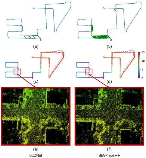
Figure 9: Performance of A-LOAM with the LCDNet (left) compared to BEVPlace++ (right) on sequence 08 of the KITTI dataset. (a), (b) are detected loops (green lines) under 100% precision. x indicate the start point of the trajectory. (c), (d) show the absolute translation errors of LCDNet and BEVPlace++, respectively. (e), (f) are the optimized point cloud map by two methods at the same crossroads.

VI-E Application

We evaluate the loop closing performance of BEVPlace++ and LCDNet by integrating these methods into a state-of-the-art LiDAR SLAM system, i.e. A-LOAM. We conduct our evaluation on sequence “08” of the KITTI dataset, which features challenging reverse loops.

In loop closing, it is crucial to detect more true loops without false positives. Therefore, we adopt the maximum recall at 100% precision as a criterion and only use true positive loops under this condition. Fig.9 (a) and (b) show the detected loops of LCDNet and BEVPlace++, respectively. As seen, BEVPlace++ detects more loops than LCDNet. This higher detection rate indicates that BEVPlace++ is more effective at identifying true loop closures, which is essential for maintaining the integrity and accuracy of the overall localization and mapping system. Fig.9 (c) and (d) illustrate the absolute translation errors of the SLAM trajectories after pose graph optimizations. BEVPlace++ achieves better accuracy. Fig.9 (e) and (f) show the optimized point cloud maps. As can be seen, the road in Fig.9 (f) is clearer, and the walls are sharper, validating that the map optimized with loops from BEVPlace++ is more accurate.

VI-F Understanding BEVPlace++

The design of REM. We conduct experiments to explore the performance of BEVPlace++ with different designs in the feature encoder. We replace the local feature encoder REM with a ResNet34 [26] and test the method on the rotated KITTI dataset to validate the significance of the rotation equivariance design. Additionally, we use different backbone CNNs in REM to study the robustness of BEVPlace++ to various backbones. Tab. X presents the place retrieval and pose estimation results of BEVPlace++ on KITTI. From Tab. X, we can conclude three observations:

• The REM is crucial for achieving robust pose estimation. As shown in Tab. X, BEVPlace++ attains higher recall rates for retrieval when using REM encoders and achieves moderate recall rates when using the ResNet encoder. However, the success rates of pose estimation drop significantly when using ResNet34 alone without our REM. This is expected, as the CNN feature map changes considerably with the orientation of the BEV image, making feature matching more challenging. In contrast, the rotation equivariance design of REM aids in pose estimation under large view changes, as the REM feature map is robust to rotational transformations.

• BEVPlace++ is robust to the choice of CNN backbone in REM. It achieves the best place retrieval recalls and pose estimation success rates when using ResNet34 as the backbone in REM. However, the performance differences when using VGG16 [59], MobileNet [69], and EfficientNet [60] as CNN backbones in REM are not significant.

TABLE X: Place retrieval and pose estimation performance of BEVPlace++ using different feature encoders

	KITTI 00
	Recall(%)	SR(%)	$\bar{e}_{t}$ (m)	$\bar{e}_{r}$ (∘)
ResNet34	99.4	64.7	0.95	1.13
REM(VGG16)	99.6	100.0	0.15	0.12
REM(MoblieNet)	99.4	99.7	0.29	0.29
REM(EfficientNet)	99.4	99.8	0.32	0.18
REM (ResNet34)	99.7	100.0	0.16	0.17
	KITTI 08
	Recall(%)	SR(%)	$\bar{e}_{t}$ (m)	$\bar{e}_{r}$ (∘)
ResNet34	92.5	60.2	0.77	1.01
REM(VGG16)	96.6	97.0	0.58	0.61
REM(MoblieNet)	94.5	96.8	0.62	0.72
REM(EfficientNet)	94.9	95.7	0.59	0.69
REM (ResNet34)	97.3	98.5	0.54	0.57

Parameter sensitivity. There are two main parameters in the BEVPlace++ network: the number of rotations $N_{R}$ in the REM module and the number of clusters $K$ in NetVLAD. We design two independent experiments on KITTI, with each experiment varying only one parameter, to discover the influence of these parameters. As shown in Tab. XI, the recall rate increases with the number of orientation intervals $N_{R}$ and tends to saturate when $N_{R}\geq 8$. This is reasonable since more accurate rotation equivariance for local features is achieved with larger $N_{R}$. Considering both computational complexity and localization recall, we set $N_{R}=8$. The recall rate increases with the number of NetVLAD clusters $K$, but does not show significant improvement when $K\geq 64$. Therefore, we set $K=64$.

TABLE XI: The recall rates of global localization under different parameter settings of REIN

The results of REM parameter $N_{R}$, fix $K=64$
Seq.	00	02	05	06	08	mean
$N_{R}=2$	99.71	88.39	98.65	99.63	92.54	95.78
$N_{R}=4$	99.56	93.87	99.10	100.0	95.22	97.55
$N_{R}=6$	99.85	94.84	99.33	99.63	97.61	98.25
$N_{R}=8$	99.71	97.10	98.88	100.0	97.31	98.60
$N_{R}=10$	99.85	98.71	99.10	100.0	96.52	98.82
The results of the cluster parameter $K$, fix $N_{R}=8$
Seq.	00	02	05	06	08	mean
$K=2$	99.71	78.71	96.41	99.26	84.48	91.71
$K=16$	100.0	94.19	98.43	100.0	97.31	97.99
$K=32$	100.0	94.84	99.33	100.0	95.82	98.00
$K=64$	99.71	97.10	98.88	100.0	97.31	98.60
$K=80$	99.85	97.21	98.66	99.63	98.21	98.71

TABLE XII: Global localization results under different settings of BEV grid

Seq.	00			08
	SR(%) $\uparrow$	$\bar{e}_{t}$ (m) $\downarrow$	$\bar{e}_{r}$ (∘)	SR(%) $\uparrow$	$\bar{e}_{t}$ (m) $\downarrow$	$\bar{e}_{r}$ (∘) $\downarrow$
$g=0.1$	100.0	0.09	0.11	99.1	0.38	0.47
$g=0.2$	100.0	0.08	0.10	98.5	0.38	0.33
$g=0.4$	100.0	0.11	0.07	98.5	0.34	0.57
$g=0.6$	99.0	0.31	0.17	96.6	0.42	0.60
$g=0.8$	98.7	0.44	0.25	95.5	0.63	0.87

The grid size $g$ is the key parameter to BEV image generation. We conduct experiments on sequences “00” and “08” to evaluate its influence on global localization. As shown in Tab. XII, The success rate decreases and the mean translation and rotation errors tend to increase as the grid size gets large. This is intuitive since the size of the BEV image will get small and the image contents will be highly compressed. We set $g\geq 0.4$ in our experiments by trading between accuracy and computation complexity.

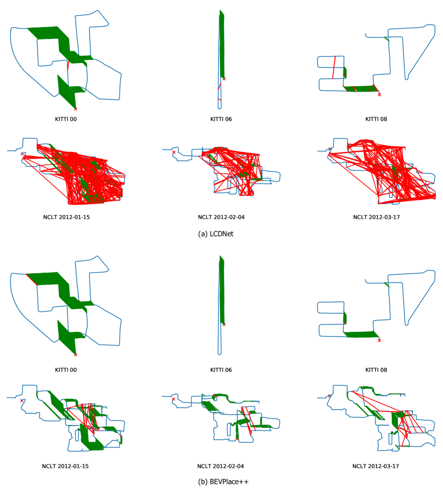
Figure 10: Comparison of detected loops of LCDNet and BEVPlace++. Green lines indicate true positives and red lines indicate false positives. x is the start point of the trajectories.

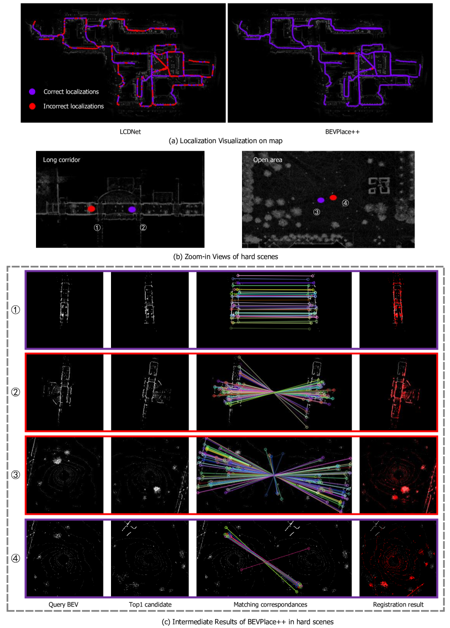
Figure 11: Visulization of the localization results of sequence 2012-02-25 of NCLT. (a) shows the correct (colored purple) and incorrect localizations (colored red) of LCDNet and BEVPlace++. (b) Zoom-in views of hard scenes for localization. (c) The intermediate localization results of BEVPlace++ including the query BEV, the top-1 candidate of place retrieval, the feature matching correspondence, and the registration results. The query BEV is colored red for better visualization.

More qualitative results. We present the detected loops of BEVPlace++ and LCDNet on the evaluation sequences in Fig. 10. In these figures, green lines indicate true positives and red lines indicate false positives. On KITTI, BEVPlace++ detects many correct loops. Notably, in the challenging sequence ”08”, BEVPlace++ successfully detects correct loops in reverse or cross routes. On the contrary, LCDNet detects more false positive loops. On the NCLT dataset, BEVPlace++ detects more false positive loops than on KITTI. The reasons are twofold. First, the point clouds in NCLT are more sparse due to the use of a sparse LiDAR scanner. Second, NCLT contains many challenging areas, such as long corridors and large open spaces, where BEV images lack significant texture information, reducing the distinctiveness of BEV features. Nevertheless, BEVPlace++ generalizes on NCLT much better than LCDNet.

Fig. 11 (a) visualizes the results of localizing the point clouds from sequence 2012-02-25 on the global map of NCLT using BEVPlace++ and LCDNet. It demonstrates that BEVPlace++ can successfully perform global localization in more areas than LCDNet. The failed localizations (colored red) of BEVPlace++ primarily occur in challenging scenes such as long corridors and open areas with few measurements. We provide a zoomed-in view of these challenging scenes in Fig. 11 (b) to better illustrate the difficulties in localization. Fig. 11 (c) further shows intermediate results of BEVPlace++ in these hard scenes, including the query BEV, the top-1 candidate for place retrieval, feature matching correspondence, and warp results. In ① and ④ of Fig. 11 (c), BEVPlace++ retrieves false top-1 candidates for the query. In both cases, the query BEV images lack sufficient structural information, hindering BEVPlace++ from extracting global descriptors with enough distinctiveness. In contrast, ② and ③ are examples where BEVPlace++ successfully localizes the queries despite significant view changes.

VII Conclusion

In this paper, we introduce BEVPlace++, a novel global localization method. BEVPlace++ adopts a two-stage method paradigm, sequentially performing place recognition and pose estimation. Utilizing BEV images, BEVPlace++ employs the rotation-equivariant network (REM) to extract robust local features. It generates rotation-invariant global descriptors with NetVLAD pooling. As a complete global localization method, BEVPlace++ can perform multiple localization tasks including place retrieval, loop closing, and global localization. A key insight of BEVPlace++ is that CNNs inherently extract distinctive features from BEV images, as demonstrated through statistical analysis under translation movements. The proposed REM enhances this distinctiveness under rotational transformations. Leveraging these characteristics, BEVPlace++ enables pose estimation for point clouds without explicit pose supervision and adapts well to diverse LiDAR scanners and unknown environments. We conducted experiments across five public datasets, showcasing BEVPlace++’s state-of-the-art performance. Additionally, we integrated BEVPlace++ as a loop closing module in a SLAM system, verifying its effectiveness in handling loop closing tasks. Concise Python APIs of our BEVPlace++ have been open-source to contribute to the robotics community. We hope BEVPlace++ will become a promising new paradigm LiDAR global localization.

Lun Luo received his B.E. and Ph.D degrees from the College of Information Science and Electronic Engineering of Zhejiang University in 2018, and 2023, respectively. He is currently a researcher in the perception algorithm of Haomo.AI Technology Co., Ltd. His research interests are localization and robot perception.

Si-Yuan Cao received his B.Eng. degree in electronic information engineering from Tianjin University in 2016, and Ph.D. degree in electronic science and technology from Zhejiang University in 2022. He is currently a lecturer in Ningbo Innovation Center, Zhejiang University, China. His research interests are homography estimation, place recognition, and image processing.

Xiaorui Li is a graduate student at Beihang University. She obtained her B.E. degree from Tianjin University in 2018. Her research interests are localization and image detection.

Jintao Xu received the Ph.D. degree in control science and engineering from Xi’an Jiaotong University, Xi’an, China, in 2016. He is currently the Director of algorithm with Haomo.AI.

Rui Ai received a Ph.D. degree in Pattern Recognition and Intelligent Systems from the Chinese Academy of Sciences in 2013. He is currently the Vice President of Haomo Technology Co., Ltd., and leads the AI Center of Haomo. He is responsible for the research and development of high-level autonomous driving systems, unmanned delivery vehicles, and data intelligence.

Zhu Yu received his B.E. degree from Zhejiang University in 2021. He is now studying for his Ph.D. degree in Zhejiang University. His research interests include depth estimation, localization, and image processing.

Xieyuanli Chen is an Associate Professor at the National University of Defense Technology, China. He received his Ph.D. degree at the Photogrammetry and Robotics Laboratory at the University of Bonn. He received his Master’s degree in Robotics in 2017 at the National University of Defense Technology. He received his Bachelor’s degree in Electrical Engineering and Automation in 2015 at Hunan University. He serves as Associate Editor for IEEE RA-L, ICRA, and IROS. His research interests are SLAM, localization, mapping, and robot perception.

References

- [1] C. Cadena, L. Carlone, H. Carrillo, Y. Latif, D. Scaramuzza, J. Neira, I. Reid, and J. J. Leonard, “Past, present, and future of simultaneous localization and mapping: Toward the robust-perception age,” IEEE Transactions on Robotics, vol. 32, no. 6, pp. 1309–1332, 2016.
- [2] R. Mur-Artal and J. D. Tardós, “Orb-slam2: An open-source slam system for monocular, stereo, and rgb-d cameras,” IEEE transactions on robotics, vol. 33, no. 5, pp. 1255–1262, 2017.
- [3] P. Dellenbach, J.-E. Deschaud, B. Jacquet, and F. Goulette, “Ct-icp: Real-time elastic lidar odometry with loop closure,” in Proceedings of the International Conference on Robotics and Automation, pp. 5580–5586, IEEE, 2022.
- [4] X. Chen, A. Milioto, E. Palazzolo, P. Giguere, J. Behley, and C. Stachniss, “Suma++: Efficient lidar-based semantic slam,” in Proceedings of the IEEE/RSJ International Conference on Intelligent Robots and Systems, pp. 4530–4537, IEEE, 2019.
- [5] R. W. Wolcott and R. M. Eustice, “Fast lidar localization using multiresolution gaussian mixture maps,” in Proceedings of the IEEE International Conference on Robotics and Automation, pp. 2814–2821, IEEE, 2015.
- [6] W. Lu, Y. Zhou, G. Wan, S. Hou, and S. Song, “L3-net: Towards learning based lidar localization for autonomous driving,” in Proceedings of the IEEE/CVF Conference on Computer Vision and Pattern Recognition, pp. 6389–6398, 2019.
- [7] D. Nister and H. Stewenius, “Scalable recognition with a vocabulary tree,” in Proceedings of the IEEE Computer Society Conference on Computer Vision and Pattern Recognition, vol. 2, pp. 2161–2168, IEEE, 2006.
- [8] S. Lazebnik, C. Schmid, and J. Ponce, “Beyond bags of features: Spatial pyramid matching for recognizing natural scene categories,” in Proceedings of the IEEE Computer Society Conference on Computer Vision and Pattern Recognition, vol. 2, pp. 2169–2178, IEEE, 2006.
- [9] A. Pronobis, B. Caputo, P. Jensfelt, and H. I. Christensen, “A discriminative approach to robust visual place recognition,” in Proceedings of the IEEE/RSJ International Conference on Intelligent Robots and Systems, pp. 3829–3836, IEEE, 2006.
- [10] B. Williams, M. Cummins, J. Neira, P. Newman, I. Reid, and J. Tardós, “A comparison of loop closing techniques in monocular SLAM,” Robotics and Autonomous Systems, vol. 57, no. 12, pp. 1188–1197, 2009.
- [11] D. Galvez-Lpez and J. D. Tardos, “Bags of binary words for fast place recognition in image sequences,” IEEE Transactions on Robotics, vol. 28, no. 5, pp. 1188–1197, 2012.
- [12] E. Rublee, V. Rabaud, K. Konolige, and G. Bradski, “ORB: An efficient alternative to SIFT or SURF,” in Proceedings of the International Conference on Computer Vision, pp. 2564–2571, IEEE, 2011.
- [13] D. Lowe, “Distinctive image features from scale-invariant keypoints,” International Journal of Computer Vision, vol. 20, pp. 91–110, 2004.
- [14] M. Angelina Uy and G. Hee Lee, “PointNetVLAD: Deep point cloud based retrieval for large-scale place recognition,” in Proceedings of the IEEE Conference on Computer Vision and Pattern Recognition, pp. 4470–4479, IEEE, 2018.
- [15] X. Chen, T. Läbe, A. Milioto, T. Röhling, O. Vysotska, A. Haag, J. Behley, C. Stachniss, and F. Fraunhofer, “OverlapNet: Loop closing for LiDAR-based SLAM,” in Proceedings of the Robotics: Science and Systems, 2020.
- [16] X. Chen, I. Vizzo, T. Läbe, J. Behley, and C. Stachniss, “Range Image-based LiDAR Localization for Autonomous Vehicles,” in Proceedings of the IEEE International Conference on Information and Automation, 2021.
- [17] J. Ma, J. Zhang, J. Xu, R. Ai, W. Gu, and X. Chen, “OverlapTransformer: An efficient and yaw-angle-invariant transformer network for LiDAR-based place recognition,” IEEE Robotics and Automation Letters, vol. 7, no. 3, pp. 6958–6965, 2022.
- [18] J. Ma, G. Xiong, J. Xu, and X. Chen, “CVTNet: A cross-view transformer network for place recognition using lidar data,” IEEE Transactions on Industrial Informatics, vol. 20, no. 3, pp. 4039–4048, 2024.
- [19] J. Du, R. Wang, and D. Cremers, “DH3D: Deep hierarchical 3D descriptors for robust large-scale 6-DoF relocalization,” in Proceedings of the IEEE Conference on Computer Vision and Pattern Recognition, pp. 744–762, Springer, 2020.
- [20] D. Cattaneo, M. Vaghi, and A. Valada, “Lcdnet: Deep loop closure detection and point cloud registration for lidar slam,” IEEE Transactions on Robotics, vol. 38, no. 4, pp. 2074–2093, 2022.
- [21] C. Shi, X. Chen, J. Xiao, B. Dai, and H. Lu, “Fast and accurate deep loop closing and relocalization for reliable lidar slam,” IEEE Transactions on Robotics, vol. 40, pp. 2620–2640, 2024.
- [22] R. Dubé, D. Dugas, E. Stumm, J. Nieto, R. Siegwart, and C. Cadena, “SegMatch: Segment based place recognition in 3D point clouds,” in Proceedings of the IEEE International Conference on Robotics and Automation, pp. 5266–5272, IEEE, 2017.
- [23] R. Dubé, A. Cramariuc, D. Dugas, J. I. Nieto, R. Siegwart, and C. Cadena, “Segmap: 3D segment mapping using data-driven descriptors,” in Proceedings of the Robotics: Science and Systems, 2018.
- [24] C. Yuan, J. Lin, Z. Liu, H. Wei, X. Hong, and F. Zhang, “Btc: A binary and triangle combined descriptor for 3-d place recognition,” IEEE Transactions on Robotics, vol. 40, pp. 1580–1599, 2024.
- [25] S. Thrun, “Probabilistic robotics,” Communications of the ACM, vol. 45, no. 3, pp. 52–57, 2002.
- [26] K. He, X. Zhang, S. Ren, and J. Sun, “Deep residual learning for image recognition,” in 2016 IEEE Conference on Computer Vision and Pattern Recognition (CVPR), pp. 770–778, 2016.
- [27] R. Arandjelovic, P. Gronat, A. Torii, T. Pajdla, and J. Sivic, “NetVLAD: CNN architecture for weakly supervised place recognition,” in Proceedings of the IEEE Conference on Computer Vision and Pattern Recognition, pp. 5297–5307, 2016.
- [28] K. Vidanapathirana, M. Ramezani, P. Moghadam, S. Sridharan, and C. Fookes, “Logg3d-net: Locally guided global descriptor learning for 3d place recognition,” in 2022 International Conference on Robotics and Automation (ICRA), pp. 2215–2221, 2022.
- [29] M. A. Fischler and R. C. Bolles, “Random sample consensus: a paradigm for model fitting with applications to image analysis and automated cartography,” Communications of the ACM, vol. 24, no. 6, pp. 381–395, 1981.
- [30] L. Luo, S. Zheng, Y. Li, Y. Fan, B. Yu, S.-Y. Cao, J. Li, and H.-L. Shen, “Bevplace: Learning lidar-based place recognition using bird’s eye view images,” in 2023 IEEE/CVF International Conference on Computer Vision (ICCV), pp. 8666–8675, 2023.
- [31] H. Yin, X. Xu, S. Lu, X. Chen, R. Xiong, S. Shen, C. Stachniss, and Y. Wang, “A survey on global lidar localization: Challenges, advances and open problems,” International Journal of Computer Vision, pp. 1–33, 2024.
- [32] K. Luo, H. Yu, X. Chen, Z. Yang, J. Wang, P. Cheng, and A. Mian, “3d point cloud-based place recognition: a survey,” Artificial Intelligence Review, vol. 57, no. 4, p. 83, 2024.
- [33] L. He, X. Wang, and H. Zhang, “M2DP: A novel 3D point cloud descriptor and its application in loop closure detection,” in IEEE/RSJ International Conference on Intelligent Robots and Systems, pp. 231–237, IEEE, 2016.
- [34] G. Kim and A. Kim, “Scan Context: Egocentric spatial descriptor for place recognition within 3D point cloud map,” in Proceedings of the IEEE/RSJ International Conference on Intelligent Robots and Systems, pp. 4802–4809, IEEE, 2018.
- [35] G. Kim, S. Choi, and A. Kim, “Scan context++: Structural place recognition robust to rotation and lateral variations in urban environments,” IEEE Transactions on Robotics, vol. 38, no. 3, pp. 1856–1874, 2021.
- [36] W. Zhang and C. Xiao, “PCAN: 3D attention map learning using contextual information for point cloud based retrieval,” in Proceedings of the IEEE/CVF Conference on Computer Vision and Pattern Recognition, 2019.
- [37] Z. Liu, S. Zhou, C. Suo, P. Yin, W. Chen, H. Wang, H. Li, and Y.-H. Liu, “LPD-Net: 3D point cloud learning for large-scale place recognition and environment analysis,” in Proceedings of the IEEE Conference on Computer Vision and Pattern Recognition, pp. 2831–2840, IEEE, 2019.
- [38] L. Hui, M. Cheng, J. Xie, J. Yang, and M.-M. Cheng, “Efficient 3D point cloud feature learning for large-scale place recognition,” IEEE Transactions on Image Processing, vol. 31, pp. 1258–1270, 2022.
- [39] Y. Xia, Y. Xu, S. Li, R. Wang, J. Du, D. Cremers, and U. Stilla, “SOE-Net: A self-attention and orientation encoding network for point cloud based place recognition,” in Proceedings of the IEEE Conference on Computer Vision and Pattern Recognition, pp. 11343–11352, 2021.
- [40] J. Komorowski, “MinkLoc3D: Point cloud based large-scale place recognition,” in Proceedings of the IEEE Winter Conference on Applications of Computer Vision, pp. 1789–1798, 2021.
- [41] J. Komorowski, “Improving point cloud based place recognition with ranking-based loss and large batch training,” in Proceedings of the International Conference on Pattern Recognition, pp. 3699–3705, IEEE, 2022.
- [42] Z. Fan, Z. Song, H. Liu, Z. Lu, J. He, and X. Du, “SVT-Net: A super light-weight network for large scale place recognition using sparse voxel transformers,” in Proceedings of the AAAI Conference on Artificial Intelligence, vol. 36, pp. 551–560, 2022.
- [43] T. X. Xu, Y. C. Guo, Y. K. Lai, and S. H. Zhang, “TransLoc3D : Point cloud based large-scale place recognition using adaptive receptive fields,” arXiv preprint arXiv:2105.11605, 2021.
- [44] Z. Zhou, C. Zhao, D. Adolfsson, S. Su, Y. Gao, T. Duckett, and L. Sun, “NDT-Transformer: Large-scale 3D point cloud localisation using the normal distribution transform representation,” in Proceedings of the IEEE International Conference on Robotics and Automation, pp. 5654–5660, 2021.
- [45] L. Hui, H. Yang, M. Cheng, J. Xie, and J. Yang, “Pyramid point cloud transformer for large-scale place recognition,” in Proceedings of the IEEE International Conference on Computer Vision, pp. 6078–6087, 2021.
- [46] A. Vaswani, N. M. Shazeer, N. Parmar, J. Uszkoreit, L. Jones, A. N. Gomez, L. Kaiser, and I. Polosukhin, “Attention is all you need,” in Conference and Workshop on Neural Information Processing Systems, pp. 5998–6008, 2017.
- [47] R. B. Rusu, N. Blodow, and M. Beetz, “Fast point feature histograms (FPFH) for 3d registration,” in Proceedings of the IEEE International Conference on Robotics and Automation, pp. 3212–3217, IEEE, 2009.
- [48] F. Tombari, S. Salti, and L. Di Stefano, “Unique signatures of histograms for local surface description,” in Proceedings of the European Conference on Computer Vision, pp. 356–369, Springer, 2010.
- [49] M. Bosse and R. Zlot, “Place recognition using keypoint voting in large 3D lidar datasets,” in Proceedings of the IEEE International Conference on Robotics and Automation, pp. 2677–2684, 2013.
- [50] K. Wang, S. Jia, Y. Li, X. Li, and B. Guo, “Research on map merging for multi-robotic system based on RTM,” in Proceedings of the IEEE International Conference on Information and Automation, pp. 156–161, IEEE, 2012.
- [51] T. Shan, B. Englot, F. Duarte, C. Ratti, and R. Daniela, “Robust place recognition using an imaging LiDAR,” in Proceedings of the IEEE International Conference on Robotics and Automation, pp. 5469–5475, IEEE, 2021.
- [52] L. Luo, S.-Y. Cao, B. Han, H.-L. Shen, and J. Li, “Bvmatch: Lidar-based place recognition using bird’s-eye view images,” IEEE Robotics and Automation Letters, vol. 6, no. 3, pp. 6076–6083, 2021.
- [53] Y. Cui, X. Chen, Y. Zhang, J. Dong, Q. Wu, and F. Zhu, “Bow3d: Bag of words for real-time loop closing in 3d lidar slam,” IEEE Robotics and Automation Letters, vol. 8, no. 5, pp. 2828–2835, 2023.
- [54] S. Shi, C. Guo, L. Jiang, Z. Wang, J. Shi, X. Wang, and H. Li, “Pv-rcnn: Point-voxel feature set abstraction for 3d object detection,” in 2020 IEEE/CVF Conference on Computer Vision and Pattern Recognition (CVPR), pp. 10526–10535, 2020.
- [55] R. Sinkhorn, “A relationship between arbitrary positive matrices and doubly stochastic matrices,” The annals of mathematical statistics, vol. 35, no. 2, pp. 876–879, 1964.
- [56] X. Xu, S. Lu, J. Wu, H. Lu, Q. Zhu, Y. Liao, R. Xiong, and Y. Wang, “Ring++: Roto-translation-invariant gram for global localization on a sparse scan map,” IEEE Transactions on Robotics, 2023.
- [57] S. Gupta, T. Guadagnino, B. Mersch, I. Vizzo, and C. Stachniss, “Effectively Detecting Loop Closures using Point Cloud Density Maps,” in IEEE International Conference on Robotics and Automation (ICRA), 2024.
- [58] E. Rosten and T. Drummond, “Machine learning for high-speed corner detection,” in Proceedings of the European Conference on Computer Vision, pp. 430–443, Springer, 2006.
- [59] K. Simonyan and A. Zisserman, “Very deep convolutional networks for large-scale image recognition,” in Proceedings of the International Conference on Learning Representations (Y. Bengio and Y. LeCun, eds.), 2015.
- [60] M. Tan and Q. Le, “Efficientnet: Rethinking model scaling for convolutional neural networks,” in International conference on machine learning, pp. 6105–6114, PMLR, 2019.
- [61] A. Geiger, P. Lenz, and R. Urtasun, “Are we ready for autonomous driving? the KITTI vision benchmark suite,” in Proceedings of the IEEE Conference on Computer Vision and Pattern Recognition, pp. 3354–3361, 2012.
- [62] N. Carlevaris-Bianco, A. K. Ushani, and R. M. Eustice, “University of michigan north campus long-term vision and LiDAR dataset,” The International Journal of Robotics Research, vol. 35, no. 9, pp. 1023–1035, 2016.
- [63] T.-M. Nguyen, S. Yuan, T. H. Nguyen, P. Yin, H. Cao, L. Xie, M. Wozniak, P. Jensfelt, M. Thiel, J. Ziegenbein, and N. Blunder, “Mcd: Diverse large-scale multi-campus dataset for robot perception,” in Proceedings of the IEEE/CVF Conference on Computer Vision and Pattern Recognition, 6 2024.
- [64] C. Taco and W. Max, “Group equivariant convolutional networks,” in Proceedings of the International Conference on Machine Learning, pp. 2990–2999, 2016.
- [65] W. Maddern, G. Pascoe, C. Linegar, and P. Newman, “1 year, 1000 km: The Oxford RobotCar dataset,” International Journal of Robotics Research, vol. 36, no. 1, pp. 3–15, 2017.
- [66] A. Shrivastava, A. Gupta, and R. Girshick, “Training region-based object detectors with online hard example mining,” in Proceedings of the IEEE Conference on Computer Vision and Pattern Recognition, pp. 761–769, 2016.
- [67] J. Behley, M. Garbade, A. Milioto, J. Quenzel, S. Behnke, C. Stachniss, and J. Gall, “Semantickitti: A dataset for semantic scene understanding of lidar sequences,” in 2019 IEEE/CVF International Conference on Computer Vision (ICCV), pp. 9296–9306, 2019.
- [68] Y. Peng, Z. Shiqi, G. Ruohai, C. Ivan, F. Ruijie, Z. Ji, C. Howie, and A. S. Sebastian, “ALITA: A large-scale incremental dataset for long-term autonomy,” in arXiv preprint arXiv:2105.11605, 2022.
- [69] M. Sandler, A. Howard, M. Zhu, A. Zhmoginov, and L.-C. Chen, “Mobilenetv2: Inverted residuals and linear bottlenecks,” in 2018 IEEE/CVF Conference on Computer Vision and Pattern Recognition, pp. 4510–4520, 2018.