The Quark-Nova model for FRBs: model comparison with observational data

Abstract

We utilize the Quark-Nova (QN) model for Fast Radio Bursts (FRBs; Ouyed et al. 2021) to evaluate its performance in reproducing the distribution and statistical properties of key observations. These include frequency, duration, fluence, dispersion measure (DM), and other relevant features such as repetition, periodicity, and the sad trombone effect. In our model, FRBs are attributed to coherent synchrotron emission (CSE) originating from collisionless QN chunks that traverse ionized media both within and outside their host galaxies. By considering burst repetition from a single chunk and accounting for the intrinsic DM of the chunks, we discover a significant agreement between our model and the observed properties of FRBs. This agreement enhances our confidence in the model’s effectiveness for interpreting FRB observations. One notable characteristic of our model is that QN chunks can undergo bursts after traveling significant distances from their host galaxies. As a result, these bursts appear to observers as hostless thus lacking a discernible progenitor. This unique aspect of our model provides valuable insights into the nature of FRBs. Furthermore, our model generates testable predictions, allowing for future experiments and observations to validate and further refine our understanding of FRBs.

1 Introduction

Fast Radio Bursts (FRBs) are intense and transient bursts of cosmological radio waves first discovered in 2007 (Lorimer et al. 2007; see also Thornton et al. 2013). The FRB pulse duration spans orders of magnitude from micro-seconds to seconds (e.g. Snelders et al. 2023), a frequency ranging from 110 MHz to 8 GHz (Gajjar et al. 2018; Pleunis et al. 2020) and appear to be a band-limited phenomenon (e.g. Pearlman et al. 2020; Kumar et al. 2021). Their redshifts range from $\sim 0.03$ to $z>1$ and they exhibit dispersion measures (DM) of hundreds of pc cm^-3 (Cordes & Chatterjee 2019) with typical uncertainty of $\sim 1$ pc cm^-3. At cosmological distances their estimated radio energies are $10^{38}$-$10^{40}$ ergs e.g. Petroff et al. 2019). Some FRBs are highly linearly polarized (e.g. Petroff et al. 2019 while a small fraction show significant circular polarization; e.g. Masui et al. 2015).

Over 600 FRB events have been identified with a small percentage of them classified as repeaters (e.g. CHIME/FRB Collaboration et al. 2021; Spitler et al. 2016; Fronsecra et al. 2020; CHIME/FRB Collaboration et al. 2023). One FRB shows a period of $\sim 16.3$ days and has been active and consistent for a few years (FRB 180916.J0158$+$65; Marcote et al. 2020). The repeating and non-repeating FRBs seem to show statistically different dynamic spectra. Repeaters are associated with wider bursts, narrower band spectra and show the “sad trombone” (multiple sub-bursts) effect (Pleunis et al. 2021; CHIME/FRB Collaboration et al. 2021). Also reported, is a statistical difference in the DM and extragalactic DM distributions between repeating and apparently non-repeating sources, with repeaters presumably having a lower mean DM (Andersen et al. 2023).

Precise localization has associated a dozen FRBs to host galaxies suggesting a diverse range of sources and regions from which these bursts originate while other FRBs are spatially offset from their hosts (Bannister et al. 2019; Prochaska et al. 2019a; Mannings et al. 2021; Bhandari et al. 2002; Mckinven et al. 2023). The variety of galaxy associations (Prochaska et al. 2019b), selection biases (Macquart & Ekers 2018) and propagation effects (e.g. Petroff et al. 2022) makes it hard to pinpoint the properties of an FRB progenitor. This has allowed for a plethora of models for FRBs which include the merger of compact objects (Metzger et al. 2019), magnetars (Kaspi & Beloborodov 2017; see also Cordes & Chatterjee 2019) flares from active stars (Loeb et al. 2014) and pulsars (Bera & Chengalur 2019; Connor et al. 2016). Repetition and periodicity has been attributed to different mechanisms including binary effects (e.g. Lyutikov et al. 2020) and precession (e.g. Li & Zanazzi 2021). A review of models and different emission mechanisms can be found in Platts et al. (2019) and Zhang (2023) and references therein. Models involving magnetars have support following the confirmation of a Galactic magnetar (SGR 1935$+$2154) producing FRBs (Rane et al. 202) albeit a very dim one.

FRBs remain an enigma (e.g. Cordes & Chatterjee (2019); Petroff et al. (2022) for recent reviews) which leaves room for new ideas to be explored. Here, we explore further our model for FRBs based on the Quark-Nova (QN) model as presented in detail in Ouyed et al. (2021) (hereafter, first paper). A QN is a hypothetical transition of an Neutron star (NS) to a quark star (QS) following quark deconfinement in the core of a NS induced by spin-down or mass-accretion onto the NS (Ouyed 2022a, b and references therein). The high brightness temperatures of FRBs point to coherent emission from a compact source with high energy density, and for this reason many models have invoked compact stars. Here, we argue instead that FRBs can emerge from relativistic, low-density objects (which are fragments of the QN ejecta) emitting coherent synchrotron emission (CSE); the FRB in our model.

At the heart of our model is the QN ejecta which fragments into millions of chunks as shown in Ouyed & Leahy (2009). As the chunks expand away from the QN site (see Figure 1 and Appendix A) they eventually become collisionless and prone to plasma instabilities (once they enter an ionized medium) which yield CSE with properties reminiscent of FRBs (Ouyed et al. 2021). Despite being a one-off explosive event, the QN can account for repetition in FRBs due to different chunks from the same QN seen at different viewing angles and at different arrival times (referred to as “angular repetition” in our model; see Figures and Tables in Ouyed et al. 2021). Repeating FRBs have been employed to dismiss the possibility of catastrophic events. However, it does not necessarily mean that a single occurrence cannot produce time-varying FRBs as shown in Ouyed et al. (2021) and as we confirm in this paper.

The average time delay between the QN and the supernova (SN) which gave birth to the NS is of the order of $\tau_{\rm QN}\sim 10^{8}$ years which is the time it takes the core of the NS to reach quark deconfinement (e.g. Staff, et al. 2006). I.e. the QN event is separated in time and space from the SN (see Figure 1). For time delays of only years to decades, the QN ejecta’s kinetic energy is harnessed before the chunks become collisionless yielding super-luminous SNe and GRBs, respectively (Ouyed et al. 2020). Furthermore, the time delay between the QN and when the chunks become collisionless as they travel in the ambient medium is decades. This effectively separates the QN event (i.e. the NS) and the QN compact remnant (the QS) from the FRB in time and space. Thus besides potentially being hostless (i.e. occurring in the outskirts of galaxies), FRBs according to our model should appear sourceless or progenitorless (see Figure 1).

In this second paper, we extend our investigation of the QN FRB model by taking into account:

(i) radial repetition from individual chunks from a given QN experiencing periodic CSE episodes (i.e. periodic FRBs) as they travel inside and outside their host galaxies radially away from the QN. There are three main scenarios for the resulting FRBs as illustrated in Figure B1: (a) Halo-Born-Halo-Bursting chunks (yielding one-off FRBs); (b) Disk-Born-Halo-Bursting chunks (yielding periodic FRBs); (c) Disk-Born-Disk-Bursting chunks (yielding repeating but not strictly periodic FRBs);

(ii) the chunks’ intrinsic DM and explore its role in differentiating angular and radial repeaters and its contribution to the extra-galactic DM. The simulated FRBs we present here show a good agreement between our model and observations and can account for the sad trombone effect, repeating and periodic FRBs when both radial and angular repetition are at play.

The paper is organized as follows: In §2, we discuss salient features of our model and give the relevant equations. In §3, we consider and simulate CSE emission from the QN primary chunk (i.e. along the observer line-of-sight) and compare it to FRB data. The case of CSE from multiple chunks from the same QN is presented in §4. We discuss our findings in §5 and list some testable prediction before we conclude in §6.

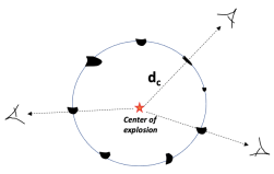
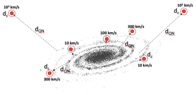
Figure 1: Left panel: The collisionless QN fragments as seen by different observers. An observer, observing many QNe will be sampling the chunk’s mass distribution. The chunks travel a distance $d_{\rm c}\sim 28.7\ {\rm pc}\times m_{\rm c,22.3}^{1/5}\Gamma_{\rm c,2.5}^{-1/5}n_{\rm amb.,-1}^{\rm ns\ -3/5}$ from the QN site before becoming collisionless. Right panel: The parent NS (experiencing the QN event) travels a distance $d_{\rm QN}^{\rm ns}=v_{\rm ckick}\tau_{\rm QN}$ before it experiences the QN event. Here, $\tau_{\rm QN}\sim 10^{8}$ years is the average time it takes for quark deconfinement in the core to set-in due to spin-down while $v_{\rm kick}$ is the NS’s natal kick velocity. A third distance in our model is $d_{\rm c,rad.}^{\rm ns}$ which is the distance travelled by the chunk between CSE episodes (see Eq. (C2)) with $d_{\rm QN}^{\rm ns}>>d_{\rm c,rad.}^{\rm ns}>>d_{\rm c}^{\rm ns}$. There are two time delays in our model: (i) the time between the birth of the NS (the supernova; SN) and when the NS experiences the QN event ($\tau_{\rm QN}\sim$ tens of millions of years yielding $d_{\rm QN}^{\rm ns}$); (ii) the time it takes the QN chunks to become collisionless ($\tau_{\rm c}\sim$ decades yielding $d_{\rm c}^{\rm ns}$).

2 our model

The energy released from the conversion of a NS of mass $M_{\rm NS}$ to a QS can be estimated as $E_{\rm QN}=(M_{\rm NS}/m_{\rm n})\times E_{\rm conv.}\sim 10^{53}$ ergs where $E_{\rm conv.}\sim 100$ MeV is the energy release per converted neutron of mass $m_{\rm n}$ (e.g. Weber 2005). The QN ejecta is the NS crust of mass $M_{\rm QN}\sim 10^{-5}M_{\rm NS}$. A small percentage $\zeta_{\rm KE}\sim 10^{-2}$-$10^{-1}$ is converted to the kinetic energy of the QN ejecta which acquires a Lorentz factor $\Gamma_{\rm QN}=\zeta_{\rm KE}E_{\rm QN}/M_{\rm QN}c^{2}\sim 10^{2}$-$10^{3}$. The average kinetic energy of the QN ejecta is thus $E_{\rm QN}^{\rm ke}\sim 10^{52}$ ergs. The compact remnant, of mass $M_{\rm QS}=(M_{\rm NS}-M_{\rm QN})\simeq M_{\rm NS}$, is a radio-quiet QS with properties summarized in Ouyed et al. (2017a, and references therein).

The QN ejecta breaks into $N_{\rm c}$ chunks with a characteristic mass $m_{\rm c}=M_{\rm QN}/N_{\rm c}\simeq 10^{22.3}\ {\rm gm}/N_{\rm c,6}$. We take $N_{\rm c}=10^{6}$ as the fiducial value and is a free parameter which varies from QN-to-QN (Ouyed & Leahy 2009). The chunk’s Lorentz factor we set to a fixed value of $\Gamma_{\rm c}=10^{2.5}$ in this work because the ejected NS crust ($M_{\rm QN}\propto M_{\rm NS}$) and the converted NS mass ($\sim M_{\rm NS}$) vary little between QNe. A typical QN chunk’s kinetic energy is $E_{\rm c}^{\rm ke}=\Gamma_{\rm c}m_{\rm c}c^{2}\sim 5.7\times 10^{45}\ {\rm ergs}\times\Gamma_{\rm c,2.5}m_{\rm c,22.3}$. The dimensionless quantities are defined as $f_{x}=f/10^{x}$ with quantities in cgs units. Unprimed quantities are in the chunk’s frame while the superscripts “ns” and “obs” refer to the NS frame (i.e. the ambient medium) and the observer’s frame, respectively.

A QN chunk moves outward from the parent NS (i.e. from the QN site) and becomes collisionless after travelling a distance $d_{\rm c}^{\rm ns}\sim 28.7\ {\rm pc}\times m_{\rm c,22.3}^{1/5}\Gamma_{\rm c,2.5}^{-1/5}n_{\rm amb.,-1}^{\rm ns\ -3/5}$ (see Eq. (A4) in Appendix A); the chunk becoming collisionless and thus prone to plasma instabilities is crucial in our model. This distance $d_{\rm c}^{\rm ns}$ is controlled by the density of the ambient environment, $n_{\rm amb.}^{\rm ns}$, where the NS experiences the QN event. The higher the $n_{\rm amb.}^{\rm ns}$ the less distance the chunk needs to travel to become collisionless. In the NS frame it takes $d_{\rm c}^{\rm ns}/c\sim 93\ {\rm years}\times m_{\rm c,22.3}^{1/5}\Gamma_{\rm c,2.5}^{-1/5}n_{\rm amb.,-1}^{\rm ns\ -3/5}$ after the QN for chunks to enter the collisionless regime.

The ambient medium can be any ionized environment in the galactic disk (e.g. the warm ionized medium; WIM), the ionized galactic halo, the intra-group/intra-cluster medium (IGpM) or the inter-galactic medium (IGM). Hereafter, the fiducial value of the ambient medium density in the NS reference frame we set to $n_{\rm amb.}^{\rm ns}=0.1$ cm^-3. It is $\Gamma_{\rm c}n_{\rm amb.}^{\rm ns}$ in the chunk’s frame.

The chunk’s number density, $n_{\rm c}$ and radius ($R_{\rm c}=(m_{\rm c}/\frac{4\pi}{3}n_{\rm c}m_{\rm H})^{1/3}$ with $m_{\rm H}$ the hydrogen mass) when it becomes collisionless were derived in Appendix SA in Ouyed et al. (2021):

$$n_{\rm c} \simeq 3.7\times 10^{3}\ {\rm cm}^{-3}\times m_{\rm c,22.3}^{1/10}\Gamma_{\rm c,2.5}^{12/5}n_{\rm amb,-1}^{\rm ns\ 6/5}$$ (1)

$$R_{\rm c} \simeq 9.3\times 10^{13}\ {\rm cm}\times m_{\rm c,22.3}^{3/10}\Gamma_{\rm c,2.5}^{-4/5}n_{\rm amb,-1}^{\rm ns\ -2/5}\ .$$

Once collisionless, the interaction with the ambient plasma protons (the beam) and the chunk’s electrons (the background plasma) triggers successively the Buneman and thermal Weibel instabilities (hereafter BI and WI) which yield CSE from the QN chunks which are FRBs in our model (see Ouyed et al. 2021). The BI converts a percentage $\zeta_{\rm BI}$ of the chunk’s electron kinetic energy to electron thermal energy in the direction of motion of the chunk yielding a temperature anisotropy which triggers the thermal WI. This anisotropy is defined by the anisotropy parameter $\beta_{\rm WI}=v_{\perp}/v_{\parallel}<1$ with $v_{\perp}$ and $v_{\parallel}$ the electron’s speed in the direction perpendicular and parallel to the chunk’s direction of motion (see Appendix B). The WI acts to remove the anisotropy by first developing current filaments within the chunk and along its direction of motion before converting the BI-gained thermal energy into magnetic energy and into accelerating the chunk’s electrons to relativistic speeds.

The filament’s initial radius is $\lambda_{\rm F,min.}=\nu_{\rm p,e}/\beta_{\rm WI}^{1/2}$ with $\nu_{\rm p,e}\simeq 9\times 10^{3}\ {\rm Hz}\times n_{\rm c,0}^{1/2}$ the chunk’s plasma frequency; $m_{\rm p}$ and $m_{\rm e}$ are the proton’s and electron’s mass, respectively. The WI filaments merge and grow in size as $\lambda_{\rm F}(t)=\lambda_{\rm F,min.}\times(1+t/t_{\rm m-WI})^{-\delta_{\rm m-WI}}$ with $t_{\rm m-WI}=\sqrt{m_{\rm p}/m_{\rm e}}\times\zeta_{\rm m-WI}/\nu_{\rm p,e}$ a characteristic timescale related to the merging and growth of WI current filaments with $\zeta_{\rm m-WI}\sim 10^{5}$ the WI filament merging parameter and $\delta_{\rm m-WI}$ the power index. The subscript “m-WI” refers the merging phase of the WI.

Electrons bunches of size $\lambda_{\rm b}$ (transverse to the direction of motion of the chunk) form around and along the WI filaments and scale linearly (and grow) with the WI filaments as $\lambda_{\rm b}(t)=\delta_{\rm b}\lambda_{\rm F}(t)$ with $\delta_{\rm b}<1$ because $\lambda_{\rm b}<\lambda_{\rm F}$. In this paper, we take $\delta_{\rm b}=1$ so that $\lambda_{\rm b}(t)=\lambda_{\rm F}(t)$ (see Appendix B). The merging amplifies the WI magnetic field and accelerates the chunks electrons yielding CSE from the bunches. The combined BI-WI tandem effectively converts kinetic energy of the chunk’s electrons to CSE (the FRB in our model) until the instability saturates and shuts-off. At any given time a bunch emits in the frequency range $\nu_{\rm p,e}\leq\nu\leq\nu_{\rm CSE,p}(t)=c/\lambda_{\rm b}(t)=c/\lambda_{\rm F}(t)$. I.e. for a given chunk, the CSE peak frequency decreases over time from $\nu_{\rm CSE,p,max.}\sim\nu_{\rm p,e}/\beta_{\rm WI}^{1/2}$ to $\nu_{\rm CSE,p,min.}=\nu_{\rm p,e}$ as $\nu_{\rm CSE,p}(t)=\nu_{\rm CSE,p,max.}\times(1+t/t_{\rm m-WI})^{-\delta_{\rm m-WI}}$.

Table 1: Fiducial parameter peak values.

$z$†	$m_{\rm c}\ ({\rm gm})^{*,\dagger}$	$n_{\rm amb.}^{\rm ns}$ (cm${}^{-3})$†	$\zeta_{\rm BI}^{\dagger}$	$\beta_{\rm WI}^{\dagger}$	$\zeta_{\rm m-WI}^{\dagger}$
0.4	$10^{22.3}$	$10^{-1}$	$10^{-1}$	$10^{-1}$	$10^{5}$

^∗ From $m_{\rm c}=M_{\rm QN}/N_{\rm c}\sim 10^{22.3}\ {\rm gm}/N_{\rm c,6}$ with $N_{\rm c}=10^{6}$ the fiducial value.
^† We consider a log-normal distribution with $\sigma(\log{x})=1.0$ for all parameters.

Table 1 lists our parameters and their fiducial values ($\delta_{\rm m-WI}$ enters later; see §3.3). These consist of the astrophysical parameters divided into the QN parameter $N_{\rm c}$ (which sets $m_{\rm c}$) and the ambient density $n_{\rm amb.}$ (which gives $n_{\rm c}^{\rm ns}$ from Eq. (1) and thus $\nu_{\rm p,e}$). The plasma parameters are $(\zeta_{\rm BI},\beta_{\rm WI},\zeta_{\rm m-WI})$, with $\zeta_{\rm BI}<1$ the percentage of electron kinetic energy converted to heat by the BI (until BI saturation), $\beta_{\rm WI}<1$ defining the size of the electron bunch $\lambda_{\rm b,min.}=\lambda_{\rm F,min.}$. The CSE peak frequency is then $\nu_{\rm CSE,p}(t)=c/\lambda_{\rm b}$(t) which decreases over time as the bunches grow in size. The parameter $\zeta_{\rm m-WI}$ sets the filament (and thus bunch) merging timescale which effectively defines the CSE characteristic duration. Variation in our model is embedded in the distribution of chunk mass (for a given QN) and ambient plasma density which portrays the different environments in which a QN can occur. Stochasticity in our model is inherent to the distribution of the plasma parameters. The CSE frequency, duration and other relevant quantities can all be expressed in terms of the chunk’s plasma frequency as shown in Appendix B.

In the observer’s frame, the frequency and time are $\nu^{\rm obs.}=\frac{D(\Gamma_{\rm c},\theta_{\rm c})}{(1+z)}\nu$ and $t^{\rm obs.}=\frac{(1+z)}{D(\Gamma_{\rm c},\theta_{\rm c})}t$. The Doppler factor is $D(\Gamma_{\rm c},\theta_{\rm c})\simeq 2\Gamma_{\rm c}/f(\theta_{\rm c})$ with $f(\theta_{\rm c})=1+(\Gamma_{\rm c}\theta_{\rm c})^{2}$ in the $\Gamma_{\rm c}^{2}>>1$ and $\theta_{\rm c}<<1$ limit; $\theta_{\rm c}$ is the viewing angle with respect to the observer’s line-of-sight (l.o.s.; see Figure A1 in Appendix A). The fluence we calculate from $\mathcal{F}=\frac{D(\Gamma_{\rm c},\theta_{\rm c})^{3}E_{\rm CSE}}{4\pi d_{\rm L}^{2}(1+z)\nu_{\rm CSE,p,max}^{\rm obs.}}$ where $d_{\rm L}$ is the luminosity distance and $z$ is the redshift; we assume a flat spectrum. Here, $E_{\rm CSE}\propto\nu_{\rm p,e}^{-2/3}$ is the energy released as CSE per BI-WI episode given by Eq. (B10) in Appendix B with $E_{\rm CSE}<<E_{\rm c}^{\rm ke}$. The chunk’s intrinsic dispersion measure (DM) as measured by the observer is DM${}_{\rm c}^{\rm obs.}=\frac{D(\Gamma_{\rm c},\theta_{\rm c})}{(1+z)}n_{\rm c}R_{\rm c}$. It is expressed in terms of the plasma frequency by using $R_{\rm c}\propto(m_{\rm c}/n_{\rm c})^{1/3}$ from Eq. (1) and $n_{\rm c}\propto\nu_{\rm p,e}^{2}$.

For a given chunk of mass $m_{\rm c}$ and Lorentz factor $\Gamma_{\rm c}$, the ambient plasma density $n_{\rm amb.}^{\rm ns}$ gives us the chunk’s number density and thus its plasma frequency $\nu_{\rm p,e}$ when it becomes collisionless. I.e.

$$\bm \simeq 0.35\ {\rm GHz}\times\frac{1}{(1+z)f(\Gamma_{\rm c},\theta_{\rm c})}\times$$ (2)

$$\times m_{\rm c,22.3}^{1/20}\Gamma_{\rm c,2.5}^{11/5}n_{\rm amb.,-1}^{\rm ns\ 3/5}\ ,$$

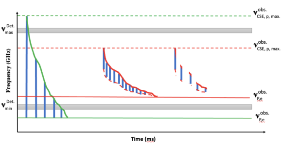
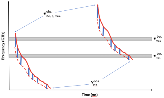
Figure B2: Top panel: Examples of CSE frequency drift in our model. The solid line depicts the $\nu_{\rm CSE,p}^{\rm obs.}(t)\propto(1+t^{\rm obs.}/t_{\rm m-WI}^{\rm obs.})^{-1}$ trend due to WI filament (and thus of electron bunches) merging and growing in size. The drift ceases when the filament size is of the order of the plasma skin depth (i.e. when $\nu_{\rm CSE,p}=\nu_{\rm p,e}$). The leftmost diagram is for a flat spectrum with drifting across the detector’s band of width $(\nu_{\rm max.}^{\rm Det.}-\nu_{\rm min.}^{\rm Det.})$. At any given time during the drifting, emission is in the frequency range $\nu_{\rm p,e}\leq\nu_{\rm CSE}\leq\nu_{\rm CSE,p}(t)$. In reality, the minimum frequency is above the plasma frequency (see Appendix B.2). I.e. the lower frequency observed in FRB detector may not reflect the chunk’s plasma frequency in particular for the case of a power-law spectrum. The middle diagram shows a power-law spectrum with the minimum and maximum CSE frequencies within the detector’s band. The right diagram shows the gaps in CSE (intermittent emission) due to the stochastic nature of WI filament (and thus bunch) merging and growth which gives rise to a “sad trombone effect” as discussed in §3.3. See Figures 1 and S4 in Ouyed et al. (2020) for other scenarios. Bottom panel: The left burst illustrates a non-repeating FRB and the right burst illustrates a repeating FRB. Repeaters in our model are CSE from chunks born in a high density ambient environment with $n_{\rm amb.}^{\rm ns}>n_{\rm amb.,c}^{\rm ns}$ (see Eq. (C3)). Their density ($n_{\rm c}\propto n_{\rm amb.}^{\rm ns\ 6/5}$) and thus their plasma frequency is higher than that of one-offs. Detectors on earth will catch the broader end of the pulse (i.e. of the filament merging process) which implies longer duration FRBS and a higher probability of experiencing a “sad trombone” effect.

with the CSE peak frequency drifting from a maximum value of $\nu_{\rm CSE,p,max.}^{\rm obs.}=\nu_{\rm p,e}^{\rm obs.}/\beta_{\rm WI}^{1/2}$ to $\nu_{\rm p,e}^{\rm obs.}$ (see Figure B2 in Appendix B).

Expressed in terms of the observed plasma frequency $\nu_{\rm p,e}^{\rm obs.}$, the key quantities in the observer’s frame (given in the chunk’s frame in Appendix B) are

$$t_{\rm m-WI}^{\rm obs.} \simeq 4.3\ {\rm ms}\times\zeta_{\rm m-WI,5}\times\frac{1}{\bm{\nu_{\rm p,e,9}^{\rm obs.}}}$$ (3)

$$\mathcal{F} \simeq 0.7\ {\rm Jy\ ms}\times\frac{\beta_{\rm WI,-1}^{1/2}\zeta_{\rm BI,-1}}{(1+z)^{5/3}f(\Gamma_{\rm c},\theta_{\rm c})^{11/3}d_{\rm L,Gpc}^{2}}\times$$

$$\times\frac{m_{\rm c,22.3}^{7/12}\Gamma_{\rm c,2.5}^{11/3}}{{\bm{\nu_{\rm p,e,9}}^{\rm obs.}}^{5/3}}$$

$$DM_{\rm c}^{\rm obs.} \simeq 286.5\ {\rm pc\ cm}^{-3}\times(1+z)^{1/3}f(\Gamma_{\rm c},\theta_{\rm c})^{1/3}\times$$

$$\times\frac{m_{\rm c,22.3}^{1/3}{\bm{\nu_{\rm p,e,9}}^{\rm obs.}}^{4/3}}{\Gamma_{\rm c,2.5}^{1/3}}$$

$$P_{\rm c,rad.}^{\rm obs.} \simeq 32.3\ {\rm days}\times\frac{1}{(1+z)f(\Gamma_{\rm c},\theta_{\rm c})}\times\frac{\Gamma_{\rm c,2.5}}{{\bm{\nu_{\rm p,e,9}}^{\rm obs.}}^{2}}\ .$$

The total CSE duration in our model is $\Delta t_{\rm CSE}^{\rm obs.}=t_{\rm m-WI}^{\rm obs.}\times(1/\beta_{\rm WI}^{1/2}-1)$ (see Appendix B).

At this point, it is important to mention that the ambient environment in which the QN event takes place, and where the chunks transition into a collisionless state, may differ from the ionized ambient medium (plasma) where the BI-WI and the FRB occur. For instance, a QN chunk can become collisionless within a neutral ambient medium in the galactic disk and subsequently emit a coherent synchrotron emission (CSE), which is identified as the FRB, when it enters an ionized medium such as the Warm Ionized Medium (WIM) in the disk, the galactic halo, the Intergalactic plasma medium (IGpM), and the Intergalactic Medium (IGM) as it moves away from the QN event; see Figure B1 in Appendix B. Once a chunk becomes collisionless, it ceases to expand and retains its plasma frequency for as long as it can emit FRBs while traversing through various ionized media. Apart from the CSE luminosity (and thus fluence), which depends on the density of the ionized medium ($n_{\rm plasma}^{\rm ns}$), all other quantities are determined by the electron plasma frequency ($\nu_{\rm p,e}$) and thus by the density of the ambient medium where the QN occurs ($n_{\rm amb.}^{\rm ns}$). See Appendix B.3 for the case of $n_{\rm plasma}^{\rm ns}\neq n_{\rm amb.}^{\rm ns}$.

2.1 Periodicity

The last equation listed above is the periodicity in the CSE emission which occurs when the ambient density $n_{\rm amb.}^{\rm ns}$ around the QN in the host galaxy exceeds a critical value (i.e. if $n_{\rm amb.}^{\rm ns}>n_{\rm amb.,c}^{\rm ns}$). As explained in Appendix C, once the WI saturates and shuts-off, electron Coulomb collisions act to dissipate the WI produced magnetic field on timescales $P_{\rm c,rad.}^{\rm obs.}$ at which point a new BI-WI episode (followed by CSE) begins.

Because the energy released as CSE during an BI-WI episode is much less than the chunk’s kinetic energy (i.e. $E_{\rm CSE}<<E_{\rm c}^{\rm ke}$), a chunk can experience many CSE episodes as it travels within or outside its host galaxy. The distance travelled by a chunk between CSE episodes is given by Eq. (C2) in Appendix C as $d_{\rm c,rad.}^{\rm ns}\simeq 39.6\ {\rm kpc}\times\frac{1}{\Gamma_{\rm c,2.5}^{7/5}m_{\rm c,22.3}^{1/10}n_{\rm amb.,-1}^{\rm ns\ 6/5}}$.

Radial repetition occurs if the length of the ambient ionized plasma $L_{\rm amb.}$ exceeds $d_{\rm c,rad.}^{\rm ns}$. This is met if $n_{\rm amb.}^{\rm ns}>n_{\rm amb.c}^{\rm ns}$ with (see Eq. (C3))

$$n_{\rm amb.,c}^{\rm ns}\sim 0.31\ {\rm cm}^{-3}\times L_{\rm amb.,10kpc}^{-5/6}\Gamma_{\rm c,2.5}^{-7/6}m_{\rm c,22.3}^{-1/12}\ .$$ (4)

This critical density separates the non-repeating chunks (i.e. radial one-offs) from repeating chunks (i.e.radial repeaters) and it is very weakly dependent on the chunk’s mass.

Radial repetition is strictly periodic if the environment is uniform along the chunk path or if neutral regions encountered by the chunk as it travels within the ambient plasma are negligible compared to $d_{\rm c,rad.}^{\rm ns}$. This makes periodic FRBs rare events which will most likely occur from chunks propagating in very low-density environments such as galactic halos, IGpM and IGM. The maximum number or periodic episodes is then $L_{\rm amb.}/d_{\rm c,rad.}^{\rm ns}$.

For example, if a chunk is born and becomes collisionless in the galactic disk where $n_{\rm amb.}^{\rm ns}\sim 1$ cm^-3 its plasma frequency is $\sim$ GHz and $d_{\rm c,rad.}^{\rm ns}\sim 1$ kpc. As it exits the galactic disk, the chunk can experience multiple CSE episodes as it crosses the galactic halo before it exits its host.

The Coulomb collision frequency is proportional to the chunk’s density $n_{\rm c}$ (i.e. $\propto\nu_{\rm p,e}^{-2}$) and is thus set once the chunk becomes collisionless. I.e. $P_{\rm c,rad.}^{\rm obs.}$ is invariant as the chunk encounters different ionized media. The chunk’s intrinsic DM (DM${}_{\rm c}^{\rm obs.}\propto\nu_{\rm p,e}^{\rm obs.\ 4/3}$) remains fixed with the only change in DM due to propagation effects. Typical change in DM due to propagation in galactic halos is $\sim(10^{-3}\ {\rm cm}^{-3})\times(10\ {\rm kpc})\sim 10$ pc cm^-3 and it is even lower if the chunk is experiencing the periodic episodes in the IGpM or in the IGM where $n_{\rm amb.}^{\rm ns}<<n_{\rm halo.}^{\rm ns}$ cm^-3.

3 The primary chunk: radial repeaters

3.1 The simulations

Consider a single chunk at a viewing angle $\theta_{\rm c}=0$ (hereafter the primary chunk) as seen by an observer (see Figure 1). For a given QN (i.e. for a given $N_{\rm c}$ and $n_{\rm amb.}^{\rm ns}$), different observers would see primary chunks with the same $\Gamma_{\rm c}$ but different mass $m_{\rm c}$. Different chunks from the same QN may encounter different plasmas as they travel away from the QN site.

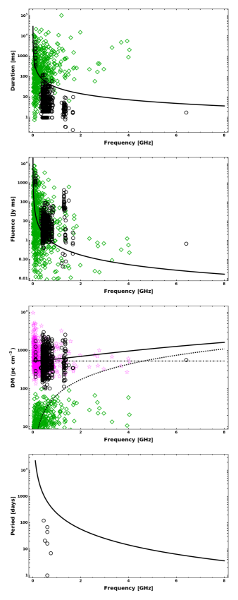
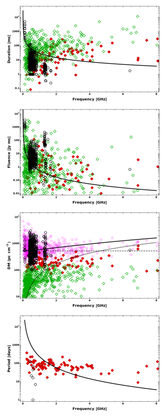
Figure 2: CSE from the primary chunks from different QNe (open green diamonds are radial one-offs; filled red diamonds are radial repeaters) compared to FRB data (open circles; from FRBSTATS website (Spanakis-Misirlis (2021)) and from CHIME Catalog 1 data (CHIME/FRB Collaboration et al. (2021))). From top to bottom: duration (ms), fluence (Jy ms), total DM (pc cm^-3) and radial period (in days) versus frequency (GHz). The solid curves are from analytical expressions given in Eq. (3) using peak values of the parameters and $\nu_{\rm CSE}^{\rm obs.}=\nu_{\rm p,e}^{\rm obs.}/\zeta_{\rm p-WI}$. In the DM panels, the dashed line is the DM${}_{\rm c}^{\rm obs.}\propto{\nu_{\rm p,e}^{\rm obs.}}^{4/3}$ from Eq. (3) while the horizontal dot-dashed line is DM${}_{\rm other}={\rm DM}_{\rm host}/(1+z)+{\rm DM}_{\rm MW}+{\rm DM}_{\rm IGM}=560$ pc cm^-3 using peak values for the parameters; the total DM is shown by the magenta stars. The left panels are for $n_{\rm amb.}^{\rm ns}=0.01$ cm^-3 and $n_{\rm amb.}^{\rm ns}=0.1$ cm^-3 in the right panels.

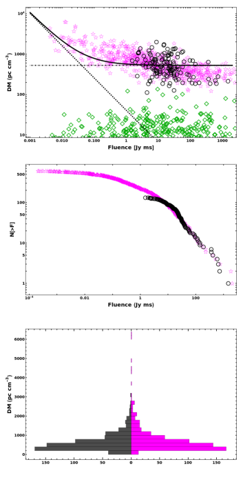
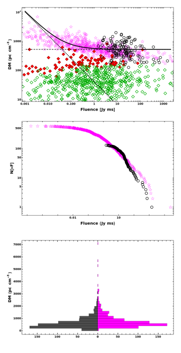
Figure 3: Top panels: Total DM in our model (magenta stars) compared to CHIME FRB (Baseband) data shown as the open circles. Radial repeaters’ DM${}_{\rm c}^{\rm obs.}$ is shown by the filled red diamonds while one-offs are the open green diamonds. The dashed line is DM${}_{\rm c}^{\rm obs.}\propto{\mathcal{F}}^{-4/5}$ from Eq. (6) while the horizontal dot-dashed line is DM${}_{\rm other}={\rm DM}_{\rm host}/(1+z)+{\rm DM}_{\rm MW}+{\rm DM}_{\rm IGM}=560$ pc cm^-3 from peak values. The analytical total DM is the solid curve. Middle panels: The cumulative distribution of burst fluences derived from the simulations (magenta stars) compared to that of CHIME’s baseband data (open circles). Bottom panels: Histograms of the simulated total DM (left half) compared to that from FRB data (right half). The left panels are for $n_{\rm amb.}^{\rm ns}=0.01$ cm^-3 and $n_{\rm amb.}^{\rm ns}=0.1$ cm^-3 in the right panels.

For all of the parameters listed in Table 1 we chose a log-normal distribution with $\sigma(\log(x))=1.0$. We set $\Gamma_{\rm c}=10^{2.5}$ and take a mean fiducial redshift value of $z=0.4$. We convert the luminosity distance using $d_{\rm L}\simeq 2z\times(2.4+z)$ (valid for $z<1$; e.g. Petroff et al. 2019 and references therein). The total DM in our model is DM${}_{\rm T}={\rm DM}_{\rm c}^{\rm obs.}+{\rm DM}_{\rm other}$ where DM${}_{\rm other}={\rm DM}_{\rm host}/(1+z)+{\rm DM}_{\rm MW}+{\rm DM}_{\rm IGM}$ is the sum of contributions from the host galaxy (DM_host), the Milky-Way galaxy (DM_MW) and the Inter-Galactic medium (DM_IGM). We take DM${}_{\rm IGM}=z\times 900$ pc cm^-3 (Yang et al. 2017) and adopt a normal distribution for the MW and host galaxy with mean $100$ pc cm^-3 and $\sigma_{\rm DM}=50$ pc cm^-3 (e.g. Taylor & Cordes 1993; Yang & Zhang 2016; Macquart et al. 2020; see also Petroff et al. 2019); we ignore possible intervening galaxies close to the l.o.s.. I.e. DM${}_{\rm other}=560$ pc cm^-3 for fiducial mean values.

In Figures 2 and 3, we compare properties of simulated CSE emission in our model to FRB data. The left panels are for $n_{\rm amb.}^{\rm ns}=0.01$ cm^-3 while $n_{\rm amb.}^{\rm ns}=0.1$ cm^-3 in the right panels. The data we use (open circles) has been retrieved from FRBSTATS website (Spanakis-Misirlis (2021)) and from CHIME Catalog 1 data (CHIME/FRB Collaboration et al. (2021)) and CHIME Baseband data (CHIME/FRB Collaboration et al. (2023)).

Figure 2 is a comparison of our model’s CSE frequency, duration, fluence and total DM to those from FRB data. The solid red diamonds show repeating primaries (i.e. periodic repeaters) while the green diamonds show the non-repeating primaries (i.e. radial one-offs). The solid curves are obtained using the parameters peak values listed in Table 1 and capture only the $\nu_{\rm CSE,p}=\nu_{\rm p,e}^{\rm obs.}/\beta_{\rm WI}^{1/2}$ dependencies as expressed in Eq. (3). The $n_{\rm amb.}^{\rm ns}=0.01$ cm^-3 simulations are dominated by radial one-offs as expected while radial repeaters make up a small percentage of the population at $n_{\rm amb.}^{\rm ns}=0.1$ cm^-3. The chunk’s DM contribution is more important at higher $n_{\rm amb.}$ (i.e. for radial repeaters) and in particular for massive chunks; DM${}_{\rm c}^{\rm obs.}\propto m_{\rm c}^{2/5}n_{\rm amb.}^{\rm ns\ 4/5}$. The bottom panels in Figure 2 show the period for radially repeating chunks (i.e. when $n_{\rm amb.}^{\rm ns}>n_{\rm amb.,c}^{\rm ns}$) versus the CSE frequency. With the $n_{\rm amb.}^{\rm ns}>n_{\rm amb.,c}^{\rm ns}$ condition inserted in $P_{\rm c,rad.}^{\rm obs.}$ in Eq. (3) we get an upper limit on the radial period of

$$P_{\rm c,rad.}^{\rm obs.}<70\ {\rm days}\times\frac{(1+z)L_{\rm amb.,10kpc}}{\Gamma_{\rm c,2.5}^{2}}\ .$$ (5)

For illustrative purposes, the analytical curve is extended above the limit in the bottom panels in Figure 2. The scatter in the simulated periods is from the $\beta_{\rm WI}$ log-normal distribution. In general primary chunks repeat only once with a “radial” period of tens of days.

The top panels in Figure 3 is the simulated DM versus fluence compared to CHIME Baseband data. The dashed curve is DM${}_{\rm c}^{\rm obs.}\propto\mathcal{F}^{-4/5}$ derived from Eq. (3) as

$$DM_{\rm c}^{\rm obs.} \simeq 207\ {\rm pc\ cm}^{-3}\times\mathcal{F}[{\rm Jy\ ms}]^{-4/5}\times$$ (6)

$$\times\frac{\beta_{\rm WI,-1}^{2/5}\zeta_{\rm BI,-1}^{4/5}\Gamma_{\rm c,2.5}^{13/15}m_{\rm c,22.3}^{4/5}}{(1+z)f(\Gamma_{\rm c},\theta_{\rm c})^{13/5}d_{\rm L,Gpc}^{8/5}}\ .$$

The solid curve is the total DM given as DM${}_{\rm T}={\rm DM}_{\rm c}^{\rm obs.}+{\rm DM}_{\rm other}$ with $D_{\rm other}=560$ pc cm^-3 for peak parameter values shown as the horizontal dot-dashed line in the top panels.

The middle panels in Figure 3 shows the Cumulative distribution of burst fluences ($N(>\mathcal{F})$) from our simulations compared to that of CHIME’s baseband data (CHIME/FRB Collaboration et al. (2023)). The $n_{\rm amb.}^{\rm ns}=0.01$ cm^-3 gave best agreement with CHIME Baseband fluence when using $\zeta_{\rm BI}=10^{-1.5}$.

Histograms of the simulated total DM compared to that from FRB data are shown in the bottom panels of Figure 3 which also shows good agreement. On average, DM${}_{\rm c}^{\rm obs.}$ is larger in radial repeaters due to the higher ambient density ($n_{\rm amb.}^{\rm ns}>n_{\rm amb.,c}^{\rm ns}$). However, this trend is reversed when considering angular repeaters (see §5).

Overall, and relying solely on the primary chunk, the agreement between our model and FRB data is encouraging. The distribution and statistical properties of most FRBs we argue is sampling the properties of CSE from primary chunks from different QNe occurring in different environments inside and outside their different host galaxies.

3.2 The chunk DM

Some FRBs show a large excess DM beyond that which is predicted by the Macquart relation (i.e. what is expected from cosmological and MW contributions; Macquart et al. (2020)). This excess could be due to the host galaxy itself, or possible foreground objects such as galaxy halos along the line-of-sight (Spitler et al. 2014; Chatterjee et al. 2017; Tendulkar et al. 2017; Hardy et al. 2017; Chittidi et al. 2020).

Figure 4 shows the extragalactic DM (DM${}_{\rm EG}={\rm DM}_{\rm IGM}+{\rm DM}_{\rm host}/(1+z)+{\rm DM}_{\rm c}^{\rm obs.}$) versus redshift in our model as compared to data (open circles; from Ryder et al. (2023)). The contribution of the repeating chunk to the DM is important in some cases and may explain the excess on its own. The estimated DM_cosmic (observed DM less Galactic and host contributions) for some observed FRBs seems to exceed the average DM_cosmic given by the Macquart relation (e.g. Simha et al. 2023). While such an excess may be within scatter in IGM DM we argue it may be due to the QN chunk’s intrinsic DM contribution. For example, for $n_{\rm amb.}=1$ cm^-3, from Eq. (3) we get DM${}_{\rm c}^{\rm obs.}\sim 446$ pc cm^-3 with $\nu_{\rm p,e}^{\rm obs.}\sim 1.4$ GHz. Higher DM${}_{\rm c}^{\rm obs.}$ can be obtained in our model by considering higher $\Gamma_{\rm c}$ values (see bullet point 4 in the predictions listed in §5).

Evidence for chunk DM contribution can be found in FRBs where the DM_host can be constrained from H_α measurements (Cordes et al. 2016) and where DM_cosmic far exceeds that derived from the Macquart relation. The variation in the total DM due to a repeating chunk propagating in the ambient plasma (e.g. the galactic halo) should not exceed $\sim n_{\rm amb.}^{\rm ns}L_{\rm amb.}\sim(10^{-3}\ {\rm cm}^{-3})\times(10\ {\rm kpc})\sim 10$ pc cm^-3. It is less if the chunk is propagating in the IGpM or in the IGM.

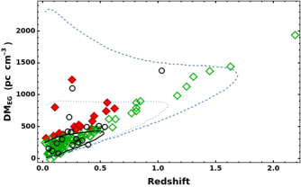
Figure 4: The extragalactic DM (DM${}_{\rm EG}={\rm DM}_{\rm IGM}+{\rm DM}_{\rm host}/(1+z)+{\rm DM}_{\rm c}^{\rm obs.}$) versus redshift from the primary chunks. The one-offs are the green diamonds while radially repeating FRBs are shown as red diamonds. The open circles are data with the curves from top to bottom showing the 99%, 90% and 50% probability for excess DM due to intervening galaxies along the line-of-sight, respectively (see Figure 3 in Ryder et al. (2023)).

3.3 The “sad trombone”

For a given electron bunch of size $\lambda_{\rm b}$, the maximum CSE frequency would drift over time towards the chunk’s plasma frequency (which remains constant) as $\nu_{\rm CSE,p}(t)=c/\lambda_{\rm b}(t)=(\nu_{\rm p,e}/\beta_{\rm WI}^{1/2})\times(1+t/t_{\rm m-WI})^{-\delta_{\rm m-WI}}$. This is illustrated in Figure B2 in Appendix B. During the turbulent merging, there are two key stochastic processes that induce intermittent CSE emission while the frequency is drifting over time: (i) the random orientation of the CSE emitting bunches until the filaments re-arrange themselves in the direction of motion of the chunk and become observable again; (ii) the intermittent acceleration of the bunches’ electrons during merging. Figure 5 shows an example of an intermittent CSE emission from a radially repeating primary chunk which reproduces the observed “sad trombone” effect in FRBs. Shown is $\nu_{\rm CSE}/\nu_{\rm CSE,p,max.}$ versus $t/t_{\rm m-WI}$ with the shaded regions showing frequency versus time for the case of a flat spectrum. Figure 6 is for the case of a power-law spectrum. The merging power index $\delta_{\rm m-WI}$ is varied using a log-normal distribution with peak value of $1$ and $\sigma{(\log{(\delta_{\rm m-WI}})})=1.0$. From a BI-WI episode to another all three scenarios of CSE (no emission, a single sub-pulse and many sub-pulses per episode) are reproduced randomly. Sub-pulses much shorter than $t_{\rm m-WI}$ (i.e. in the sub-microsecond regime in the observer’s frame where $t_{\rm m-WI}^{\rm obs.}\sim$ ms) can be reproduced while in some cases the drifting appears smooth with no interruption in the CSE. In our model, pulses as short as the bunch’s cooling timescale are possible. A bunch cools on timescales $N_{\rm e,b}\gamma_{\rm e}m_{\rm e}c^{2}/L_{\rm CSE}\sim 10^{-13}$ s where $N_{\rm e,b}$ is the number of electrons per bunch given in Appendix B.1 and $\gamma_{\rm e}\sim 10$ the electron’s Lorentz factor.

A parameter survey using primary chunks only reproduces most of the sub-pulse behavior and properties observed in repeating FRBs. Alternatively, the two figures discussed above can be interpreted as CSE emission from different one-off primary chunks from different QNe. In the spectrum, the minimum CSE frequency is the chunk’s plasma frequency while the peak frequency scales as $\nu_{\rm CSE,p,max.}=\nu_{\rm p,e}/\beta_{\rm WI}^{1/2}$. The sad trombone effect will be more prominent in repeaters because of the higher plasma frequency (from $n_{\rm amb.}^{\rm ns}>n_{\rm amb.,c}^{\rm ns}$) which means that detector will capture the longer end-tail of the pulse (see bottom panel in Figure B2). Non-repeaters will be caught by a detector earlier and would appear narrower. Because of the wider pulse, on average, the sad trombone effect is more likely to be observed in repeaters. This also explains why sub-pulses are in-band as the emission gets randomly cut-off during merging. For individual bursts both repeaters and non-repeaters show the sad trombone, but statistically, the repeaters should show it more often. However, the sad trombone may not be unique to repeaters.

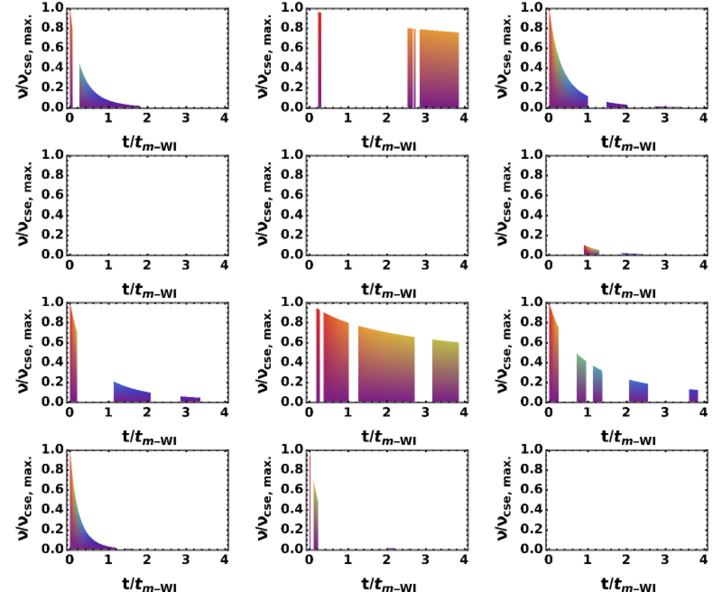
Figure 5: CSE frequency (in units of $\nu_{\rm CSE,p}^{\rm obs.}(t=0)$) versus time (in units of $t_{\rm m-WI}^{\rm obs.}$) for a radially repeating primary as it travels in its host galaxy. Contours of the normalized flux density are also shown for the case of a flat spectrum. The blank panels correspond to merging so intermittent that nothing is observed.

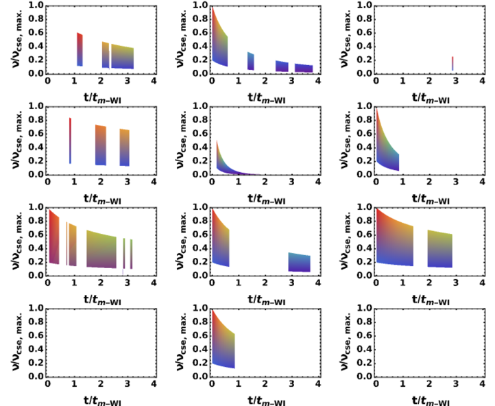
Figure 6: Same as in Figure 5 but for a power-law spectrum.

For completeness, and from $\nu_{\rm CSE,p}^{\rm obs.}=\nu_{\rm CSE,p,max.}^{\rm obs.}\times(1+t^{\rm obs.}/t_{\rm m-WI}^{\rm obs.})^{-\delta_{\rm m-WI}}$, we derive a relationship between the drifting slope and the CSE frequency

$$\frac{d\nu_{\rm CSE}^{\rm obs.}}{dt^{\rm obs.}} =-\frac{{\nu_{\rm CSE}^{\rm obs.}}^{2}}{\nu_{\rm CSE,p,max.}t_{\rm m-WI}^{\rm obs.}}$$ (7)

$$\simeq-\left(\frac{7.3\times 10^{-2}\beta_{\rm WI,-1}^{1/2}}{\zeta_{\rm m-WI,5}}{\rm GHz^{-1}ms^{-1}}\right)\times{\nu_{\rm CSE}^{\rm obs.}}^{2}\ ,$$

which should be verifiable with FRB data.

4 Multiple chunks: Angular repeaters

We now consider multiple chunks from a given QN as depicted in Figure A1 (see Appendix A). This scenario has been studied in Ouyed et al. (2021). However, in this analysis, we specifically examine the influence of the chunk’s intrinsic DM on DM_T and investigate the conditions under which“angular + radial” repetition is feasible.

The chunk closest to the line-of-sight is the primary chunk (denoted by the subscript “P”; the one discussed in the previous section). The secondary and tertiary chunks, at higher viewing angle, denoted by “S” and “T”. Each chunk from a given QN obeys the equations given in Eq. (3). A secondary and tertiary chunk differs from the primary by the mass (which is random) and the viewing angle. Because $\Gamma_{\rm c}$ is fixed, hereafter we write $f(\Gamma_{\rm c},\theta_{\rm c})=f(\theta_{\rm c})$ with a corresponding average values based on average viewing angles being $f(\bar{\theta}_{\rm S})\simeq 1+0.97\times\Gamma_{\rm c,2.5}^{2}/N_{\rm c,6}$, $f(\bar{\theta}_{\rm T})\simeq 1+6.67\times\Gamma_{\rm c,2.5}^{2}/N_{\rm c,6}$ and that of the primary is $f(\bar{\theta}_{\rm P})\sim 1+0.18\times\Gamma_{\rm c,2.5}^{2}/N_{\rm c,6}\simeq 1$ (see Appendix A).

It is instructive to rewrite the key equations in their general forms. I.e.

$$t_{\rm m-WI}^{\rm obs.} \simeq 12.3\ {\rm ms}\times\zeta_{\rm m-WI,5}\times\frac{(1+z)f(\theta_{\rm c})}{m_{\rm c,22.3}^{1/20}\Gamma_{\rm c,2.5}^{11/5}n_{\rm amb.,-1}^{\rm ns\ 3/5}}$$ (8)

$$\mathcal{F} \simeq 3.8\ {\rm Jy\ ms}\times\frac{\beta_{\rm WI,-1}^{1/2}\zeta_{\rm BI,-1}}{(1+z)f(\theta_{\rm c})^{2}d_{\rm L,Gpc}^{2}}\times\frac{m_{\rm c,22.3}^{1/2}}{n_{\rm amb.,-1}^{\rm ns}}$$

$$DM_{\rm c}^{\rm obs.} \simeq 71.2\ {\rm pc\ cm}^{-3}\times\frac{m_{\rm c,22.3}^{2/5}\Gamma_{\rm c,2.5}^{13/5}n_{\rm amb.,-1}^{\rm ns\ 4/5}}{(1+z)f(\theta_{\rm c})}$$

$$P_{\rm c,rad.}^{\rm obs.} \simeq 267.8\ {\rm days}\times\frac{(1+z)f(\theta_{\rm c})}{m_{\rm c,22.3}^{1/10}\Gamma_{\rm c,2.5}^{17/5}n_{\rm amb.,-1}^{\rm ns\ 6/5}}$$

$$P_{\rm c,ang.}^{\rm obs.} \simeq 3.0\ {\rm hrs}\times(1+z)\times\frac{m_{\rm c,22.5}^{1/5}}{N_{\rm c,6}\Gamma_{\rm c,2.5}^{1/5}n_{\rm amb,-1}^{\rm ns\ 3/5}}\ .$$

We added the last equation which is the average angular time separation, $P_{\rm c,ang.}^{\rm obs.}$, between chunks which is independent of $f(\theta_{\rm c})$ (see Appendix A). Except for $\mathcal{F}\propto m_{\rm c}^{1/2}$ and DM${}_{\rm c}^{\rm obs.}\propto m_{\rm c}^{2/5}$, all other quantities are weakly dependent on the chunk’s mass; $n_{\rm amb.}^{\rm ns}$ is fixed for a given QN. The two quantities which are prone to the most scatter are $t_{\rm m-WI}^{\rm obs.}$ (and thus the FRB duration) and $\mathcal{F}$ due to their dependency on the stochastic plasma parameters.

For $n_{\rm amb.}^{\rm ns}<n_{\rm amb.,c}^{\rm ns}$ and $N_{\rm c}\sim 10^{6}$, we get the regime of angular repetition where the chunks DM is negligible because $f(\theta_{\rm c})>>1$. In this case, all emitting chunks from a given QN would be associated with the same total DM given by DM${}_{\rm T}={\rm DM}_{\rm other}>>{\rm DM}_{\rm c}^{\rm obs.}$. Also, there is no change in DM_T because the chunks emit once. However, angular repetition is at best quasi-periodic and even irregular because the chunks are not precisely equally spaced and the variation in $f(\theta_{\rm c})$ between chunks is somewhat variable (see Ouyed et al. (2021)). Below we focus on the $n_{\rm amb.}^{\rm ns}>n_{\rm amb.,c}^{\rm ns}$ scenario where all chunks from a given QN repeat radially.

4.1 Simulations

In the NS frame, the distance travelled by any chunk between BI-WI episodes, $d_{\rm c,rad.}^{\rm ns}$, is independent of the viewing angle and it is the same for all chunks for a given QN (see Eq.(C2)). It is also very weakly dependent on mass ($\propto m_{\rm c}^{-1/10}$). This means that if the primary is a radial repeater then all peripheral (here S and T) chunks will also be radial repeaters. Periodicity form multiple chunks ensue as long as the environment along each chunk’s path is the same.

Figure 7 shows periodic FRBs from the primary, secondary and tertiary chunks for fiducial parameter values (see Table 1). The columns from left to right are for $n_{\rm amb.}^{\rm ns}({\rm cm}^{-3})=(0.1,1.0,10.0)$; only three periods are shown. From top to bottom are, the frequency, duration, fluence, chunks’ DM, all as solid circles, versus time (in days). The total DM in the bottom panels is shown with the open stars. For fiducial values we have $f(\theta_{\rm P})\sim 1,f(\theta_{\rm S})\sim 2,f(\theta_{\rm T})\sim 7$ which helps in clearly distinguishing the primary, secondary and tertiary chunks via the viewing angle effect in the frequency (despite $\nu_{\rm p,e}\propto m_{\rm c}^{1/20}$) and DM (despite DM${}_{\rm c}^{\rm obs.}\propto m_{\rm c}^{2/5}$) panels. They are less distinguishable in the duration and fluence panels due to their dependence on the stochastic plasma physics parameters. For $n_{\rm amb.}^{\rm ns}=0.1$ cm^-3 the variation in chunks total DM is narrower but it is still noticeable. As $n_{\rm amb.}^{\rm ns}$ increases, DM${}_{\rm c}^{\rm obs.}\propto n_{\rm amb.}^{\rm ns\ 4/5}$ becomes more important and the main contribution to the total DM varies widely between chunks. In this scenario, all chunks repeat radially and despite belonging to the same QN (i.e. the same FRB source) they could be interpreted as being from different sources and located at different distances. The angular repetition timescales, from the left to the right column are $P_{\rm c,ang.}^{\rm obs.}\propto n_{\rm amb.}^{\rm ns\ -3/5}\sim 3$ hours, 0.76 hours and 0.2 hours, respectively.

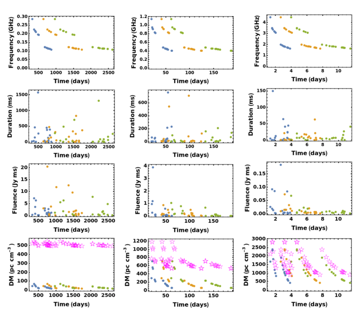
Figure 7: FRBs from the primary, secondary and tertiary chunks for $n_{\rm amb.}^{\rm ns}=(0.1,1.0,10.0)$ cm^-3 (from left to right). Other parameters were set to fiducial values with their log-normal distributions when applicable (see §4). The bottom panels show the total DM (magenta stars) and the chunks’ DM as filled circles. Three periodic episodes are shown with chunks color blue, orange and green, respectively, in each panel. We assume conditions are met for periodic repetition to occur where neutral regions within the ambient plasma are negligible in size compared to $d_{\rm c,rad.}^{\rm ns}$.

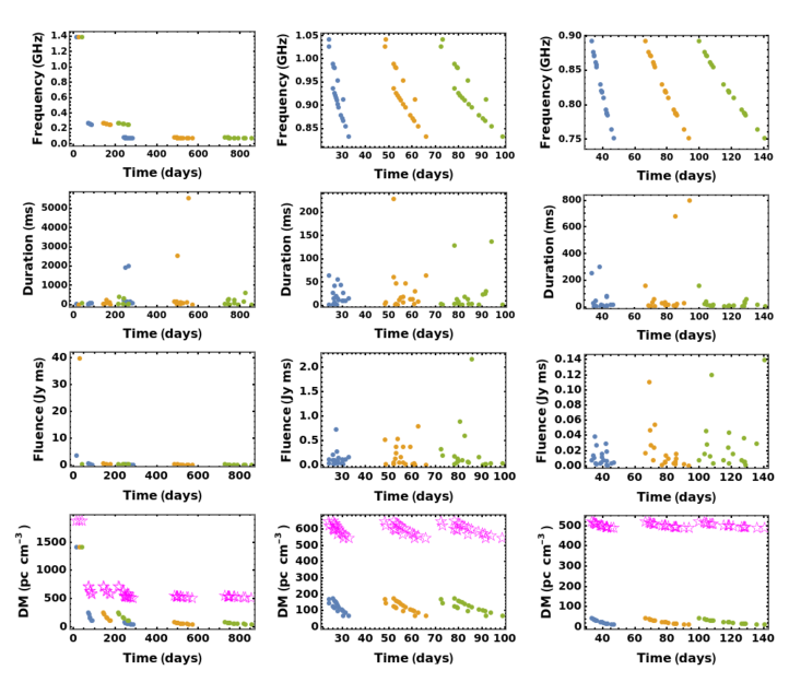
Figure 8: FRBs from the primary, secondary and tertiary chunks for $n_{\rm amb.}^{\rm ns}=1$ cm^-3 and $N_{\rm c}=(10^{5},10^{7},10^{9})$ (from left to right). Other parameters were set to fiducial values with their log-normal distributions when applicable (see §4). The bottom panels show total DM (magenta stars) and the chunks’ DM as filled circles. Three periodic episodes are shown with chunks color blue, orange and green, respectively, in each panel.

For chunks from the same QN, to have the same intrinsic DM would require $f(\theta_{\rm c})\sim 1$. This is the case up to the tertiary chunks if $N_{\rm c}>N_{\rm c,c}=10^{8}\Gamma_{\rm c,2.5}^{2}$ where the effect of the viewing angle are negligible. In this case, the total DM is the same for S, P and T chunks with variations in total DM, $\Delta(DM_{\rm T})=n_{\rm amb.}^{\rm ns}L_{\rm amb.}\sim$ pc cm^-3, due to propagation in the ambient plasma.

Figure 8 shows periodic FRBs from the primary, secondary and tertiary chunks for $n_{\rm amb.}^{\rm ns}=1.0$ cm^-3 while other parameters are kept to their fiducial values (see Table 1). The columns from left to right are for $N_{\rm c}=(10^{5},10^{7},10^{9})$; only three periods are shown. From top to bottom are, the frequency, duration, fluence, chunks’ DM, all as solid circles, versus time (in days). The total DM in the bottom panels is shown with the open stars. The spread in the period between different chunks is more apparent at low $N_{\rm c}$ as expected because $P_{\rm c,rad.}^{\rm obs.}(\theta_{\rm c})\propto f(\theta_{\rm c})$ and $f(\theta_{\rm c})>>1$. We see that as $N_{\rm c}$ increases and the $\theta_{\rm c}$ dependence is removed (i.e. $f(\theta_{\rm c})\sim 1$), all chunks behave as primaries. One consequence is the narrowing in the frequency range and in the radial period range. This leaves the $m_{\rm c}$ dependence DM${}_{\rm c}^{\rm obs.}\propto m_{\rm c}^{2/5}$ so that for the larger $N_{\rm c}$ case the chunk’s intrinsic DM can be negligible and all chunks would be associated with the same total DM. Because the angular period scales as $P_{\rm c,ang.}\propto N_{\rm c}^{-6/5}$, it varies from $\sim 12$ hours when $N_{\rm c}=10^{5}$ to $\sim 0.76$ s when $N_{\rm c}=10^{9}$.

Table 2: An 16.3 day periodic repeater in our model (reproducing FRB 180916.J0158$+$65)

^† The corresponding chunk DM is DM${}_{\rm c}^{\rm obs.}\sim 70$ pc cm^-3.

4.2 An 16.3 day strictly periodic repeater

We find that FRB 180916.J0158$+$65 is best explained in our model if the QN occurred in the disk of its host galaxy and burst in its outskirts (the halo of the IGpM). I.e. FRB 180916.J0158$+$65 is a Disk-Born-Halo-Bursting FRB which yields strictly periodic FRBs in our model. In this picture, a primary chunk is travelling away from the host’s disk in the low-density halo or IGpM towards the observed. This is a plausible scenario because the host of FRB 180916.J0158$+$65 is a spiral seen nearly face-on (Marcote et al. 2020) so we could be seeing the primary heading towards us away from its birth place in the disk. We recall that the CSE frequency and all other quantities (in particular its 16.3 day period) which depend on the chunk’s plasma frequency were set by where the chunk was born; here the disk of the spiral galaxy.

The 16.3 day periodic FRB 180916.J0158$+$65 (at redshift $z=0.0337$) can be reproduced using the parameters listed in Table 4.1. Other parameters were kept to their fiducial peak values and varied following a log-normal distribution as before. The three columns in Figure 9 are for $\sigma(\log{(m_{\rm c})})=0.01,0.1$ and 1.0 from left to right, respectively. A narrow chunk mass distribution is necessary to reproduce properties of the observed 16.3 day FRB with $N_{\rm c}=10^{8}$ so that $f(\theta_{\rm c})\sim 1$ up to at least the tertiary chunks. Because $P_{\rm c,rad.}^{\rm obs.}\propto\nu_{\rm CSE}^{\rm obs.\ -2}$ (see Eq. (3)), the periodicity is chromatic with the higher frequency FRBs arriving first. The few days activity window is due to the chunks mass distribution.

The resulting chunks’ DM is DM${}_{\rm c}^{\rm obs.}\simeq 70$ pc cm^-3 while DM${}_{\rm IGM}=z\times 900\simeq 30$ pc cm^-3. By taking DM${}_{\rm MW}=150$ pc cm^-3 and DM${}_{\rm host}=100$ pc cm^-3 we get a total DM of DM${}_{\rm T}\sim 350$ pc cm^-3 for all chunks. This number agrees with the measured DM in FRB 180916.J0158$+$65. The distance travelled per period by a QN chunk in its host galaxy is $d_{\rm c,rad.}^{\rm ns}\sim 1.8$ kpc. According to our model, FRB 180916.J0158$+$65 will be active for $\frac{L_{\rm amb.}}{d_{\rm c,rad.}^{\rm ns}}\times 16.3\ {\rm days}$ which is few years for $L_{\rm amb.}\sim 10$ kpc. A much longer activity is possible if the chunk is travelling in the IGpM.

Figure 10 shows the Cumulative distribution of burst fluences derived from our simulations compared to that of FRB 180916.J0158$+$65 baseband data (Marcote et al. (2020)) which shows good agreement. We also note that the angular time delay between chunks is $P_{\rm c,ang.}^{\rm obs.}\sim 8.8$ s. Finally, in Figures 11 (for a flat spectrum) and Figures 12 (for a power-law spectrum) we give examples of sub-pulses and the sad trombone effect from one of the chunks as it experiences 12 CSE episodes. Alternatively, the figures can be associated with CSE emission from 12 different chunks at different viewing angles.

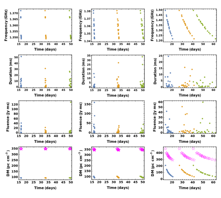
Figure 9: An $\sim 16.3$ days repeater in our model with parameters given in Table 4.1. The three columns are for $\sigma(\log{(m_{\rm c})})=0.01,0.1$ and 1.0 from left to right. Other parameters were set to fiducial values with their log-normal distributions when applicable (see §4). The bottom panels shows total DM (magenta stars) and the chunks’ DM as filled circles. Three periodic episodes are shown with chunks color blue, orange and green, respectively, in each panel.

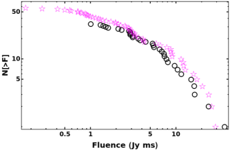
Figure 10: The cumulative distribution of burst fluences derived from the 16.3 day-FRB simulation in our model (magenta stars) compared to that of CHIME’s FRB 180916.J0158$+$65 data (open circles).

Figure 11: CSE frequency (in units of $\nu_{\rm CSE,p}^{\rm obs.}$) versus time (in units of $t_{\rm m-WI}^{\rm obs.}$) for a sample of secondary and tertiary chunks from the 16.3 days CSE simulation.

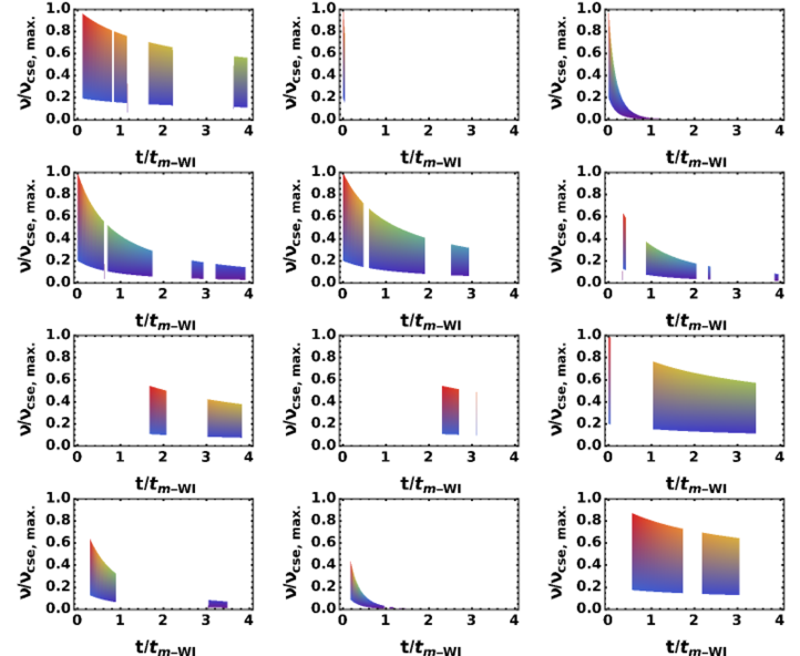
Figure 12: Same as in Figure 11 but for a power-law spectrum.

5 Discussion and testable predictions

We start by discussing some distinctive features of our model:

• The overall FRB rate: In a galaxy like ours, roughy $1$% of all neutron stars formed over a Hubble time experience a QN episode (Ouyed et al. 2020). With a core-collapse supernova (ccSN) rate of $10^{-2}$ per year per high mass ($L_{\star}$) galaxy, about $\sim 10^{-2}\ {\rm yr}^{-1}\times 10^{10}\ {\rm yr}=10^{8}$ NSs have formed with $\sim 10^{6}$ NSs as QN candidates. The QN rate in our model per year per galaxy is thus $10^{6}/10^{10}\ {\rm yr}=10^{-4}\ {\rm yr}^{-1}$ per galaxy or $\sim 2.7\times 10^{-7}\ {\rm day}^{-1}$ per galaxy. Over the whole sky (with $\sim 10^{11}$ galaxies) we get a rate of $\sim 2.7\times 10^{4}$ per day. The intrinsic FRB rate is much higher by $N_{\rm c}$; but of these only a fraction are observed in any given direction because of beaming. For $\Gamma_{c}=10^{2.5}$, the beaming factor is $\sim 10^{-5}$ but also depends on how sensitive the detector is. I.e. fewer bursts seen at larger distance from the observer. We used $10^{11}$ galaxies to estimate the QN rate but what matters is the number of galaxies within the upper detection distance of FRBs. Nevertheless, within an order of magnitude we arrive at an FRB rate which is similar to the observed rate. A similar rate was derived in Ouyed et al. (2021) based on a more rigorous calculation.

• The repeating FRBs rate: The parent NS travels a distance $d_{\rm QN}^{\rm ns}$ from its birth site before it experiences a QN event (see right panel in Figure 1). Here, $d_{\rm QN}^{\rm ns}=v_{\rm kick}\tau_{\rm QN}$ with $\tau_{\rm QN}\sim 10^{8}$ years the average time it takes for quark deconfinement in the core to set-in due to spin-down (e.g. Staff, et al. (2006)) and $v_{\rm kick}$ the NS’s natal kick velocity. Assuming a distribution peaking at $v_{\rm kick}\sim 300$ km s^-1 (e.g. Faucher-Giguère & Kaspi 2006), most NSs would have travelled 30 kpc from their birth site when they experience the QN event. I.e. most QNe from old spinning-down NSs would occur in an $n_{\rm amb.}^{\rm ns}<<n_{\rm amb.,c}^{\rm ns}$ environment within their galaxies yielding one-off FRBs. The low $v_{\rm kick}$ NSs would experience the QN in the densest environment in their host galaxies (i.e. while still in the disk) and should yield repeating FRBs. These, and taking $v_{\rm kick}$ of a few km s^-1, would correspond to a small percentage of the total population of FRBs. On the other hand, NSs with $v_{\rm kick}>10^{3}$ km s^-1 experiencing the QN event, would give FRBs outside their host galaxy within the intra-cluster medium and/or the IGM where ambient densities are extremely low and should translate to small fluences.

• Periodic FRBs: Periodic FRBs in our model occur when $L_{\rm amb.}>>d_{\rm c,rad.}^{\rm ns}$ and when regions of neutral gas within the ambient plasma are smaller than $d_{\rm c,rad.}^{\rm ns}$. This hints at galactic halos or Intra group media. Together with the fact that the responsible chunks must be born in relatively high ambient density (i.e. in galactic disks) makes periodic FRBs very rare events.

• The binary connection: Quark deconfinement in the core of a NS (and the ensuing QN) could also occur via mass-accretion onto the NS from a companion (e.g. in Low-MassX-ray Binaries; see Ouyed et al. (2017b, and references therein)). Some FRBs should be associated environments harbouring massively accreting NSs; e,g, in Globular clusters. Even though the FRB would occur well outside the globular cluster, it would be projected in front of it because its motion is along the line-of-sight to the globular cluster.

• FRBs in the galactic disk: In the galactic disk, FRBs occur whenever a collisionless QN chunk enters an ionized medium and may repeat if $L_{\rm plasma}>d_{\rm c,rad.}^{\rm ns}$. The most likely environment is the warm ionized medium (WIM; Hoyle & Ellis 1963) which accounts for about half of the disk’s volume (e.g. Reynolds 1991; Ferreire 2001; Haffner et al. 2009). These FRBs should in principle be associated with [CII] and [NII] in absorption towards bright continuum sources associated with the WIM (e.g. Persson et al. 2014; Gerin et al. 2015).

• FRB 20180916B and FRB 20121102A: FRBs in our model can occur in all types of galaxies and all have in common the CSE emitting collisionless QN chunks and should thus share many properties despite the different hosts.

  FRB 20121102A is best explained in our model as an angular repeater occurring in a low ambient density medium ($n_{\rm amb.}^{\rm ns}<n_{\rm amb.,c}^{\rm ns}$) with an activity lasting for decades as demonstrated in our previous paper (see Tables S5, S10 and S11 in Ouyed et al. 2021). For FRB 20190608B we favor a Disk-Born-Halo(or IGpM)-Bursting chunk scenario. Nevertheless, they should both show similarities in their FRB properties despite the striking difference between the FRB 20121102A host galaxy (a low-metallicity dwarf at $z=0.193$; Chatterjee et al. 2017) and that of FRB 20190608B (a spiral at $z=0.0337$; Marcote et al. 2020).

• Angular vs radial repeaters: (i) Angular repeaters involve chunks from the same QN but at different viewing angles. For angular repetition to occur, the QN needs to be closer in redshift. This proximity is necessary for the fluence (with $\mathcal{F}\propto f(\theta_{\rm c})^{-2}$) from peripheral chunks to be with detectors’ sensitivity. Angular repeaters are characterized by a lower DM_T due to a reduced contribution of intergalactic medium (IGM) DM and a lower DM${}_{\rm c}^{\rm obs.}\propto f(\theta_{\rm c})^{-1}$. There is no change in the total DM in this case; Radial (and periodic) repeaters occur when single chunks experience multiple CSE episodes as they travel radially away from the QN in the ambient plasma. Because $n_{\rm amb.}^{\rm ns}>n_{\rm amb.,c}^{\rm ns}$, the DM of a radially repeating chunk on average will exceed that of an angular repeater. Also, because $\theta_{\rm c}\sim 0$, a radial repeater can be detected at larger redshifts. We add that in order to experience many CSE episodes, repeaters likely occur in the halo of their hosts or outside where the ambient density extremely small; Disk-Born-Halo(or IGpM)-Bursting chunks. This should be associated with DM${}_{\rm host}\sim 0$ and very small change in DM.

• The spectrum: In our model, it is a convolution of the CSE spectrum per bunch (a boosted synchrotron spectrum in the frequency range $\nu_{\rm p,e}\leq\nu\leq\nu_{\rm CSE,p}$) and the bunch size distribution $\lambda_{\rm b}$ with $\nu_{\rm CSE,p}=c/\lambda_{\rm b}$. For a given chunk, and in the simplest possible picture, all bunches have the same size and grow as $\lambda_{\rm b}(t)\propto(1+t/t_{\rm m-WI})$. A preliminary analysis is given in Appendix D with an example spectrum given in Figure D1. However, the final spectrum is more complex when considering a distribution of bunches at any given time and their evolution due to turbulent filament merging. Furthermore, while the number of electron per bunch is constant for a given chunk (see Eq. (B1) in Appendix D), the distribution of the electron Lorentz factor $\gamma_{\rm e}$ will vary from bunch-to-bunch within a chunk. The underlying CSE spectra is more likely to be smeared out and would lose its underlying synchrotron shape (i.e. $\nu^{1/3}$ for $\nu<\nu_{\rm CSE,p}$) and should instead carry the signature of the turbulent merging of the WI filaments. A detailed analysis is beyond the scope of this paper and will be done elsewhere.

We end by listing a few testable predictions:

• FRBs as probes of ionized media in the universe: Because the CSE luminosity scales as $n_{\rm plasma}$ (see Eq. (B10) in Appendix B), as a radially repeating chunk encounters density jumps it should be reflected in the fluence. When the jumps are small such variations may be masked by the stochasticity related to the plasma parameters $\beta_{\rm WI}$ and $\zeta_{\rm BI}$. However, there are instances where the jump in $n_{\rm amb.}^{\rm ns}$ may be important enough that it can reflect directly on the fluence: (i) WIM ($n_{\rm amb.}^{\rm ns}\sim 10^{-1}$ cm^-3) to Galactic-halo ($n_{\rm amb.}^{\rm ns}\sim 10^{-3}$ cm^-3) ; (ii) Galactic-halo ($n_{\rm amb.}^{\rm ns}\sim 10^{-3}$ cm^-3) to inter-group ($n_{\rm amb.}^{\rm ns}\sim 10^{-5}$ cm^-3); (iii) inter-group ($n_{\rm amb.}^{\rm ns}\sim 10^{-5}$ cm^-3) to IGM ($n_{\rm amb.}^{\rm ns}\sim 10^{-7}$ cm^-3); (iv) The most important jump in fluence would be when a CSE emitting chunk in the halo exits the galaxy and enters the IGM. While the CSE frequency should remain the same, we expect a dimming in fluence by a factor of $n_{\rm IGM}/n_{\rm halo}\sim 10^{-4}$.

  We expect FRB 180916.J0158$+$65 to eventually dim as the emitting QN chunk enters the IGpM (if it is currently emitting in its host’s halo) or the IGM if it is currently emitting in the surrounding IGpM. In the process, its fluence will decrease by a factor of tens to hundreds while other quantities remain the same.

• Long duration FRBs: The FRB duration in our model is related to that of the WI filament merging phase with $\Delta t_{\rm CSE}^{\rm obs.}\propto(1/\beta_{\rm WI}^{1/2}-1)\times\zeta_{\rm m-WI}/\nu_{\rm p,e}$. The distribution in the astrophysical and plasma parameters yields FRBs lasting for minutes as can be seen from Figures 2, 7 and 8.

• Hostless and “sourceless/progenitor-less” FRBs: With $\tau_{\rm QN}\sim 10^{8}$ years and $v_{\rm kick}\sim 300$ km s^-1, a parent NS would have travelled tens of kilo-parsecs from its birth site before experiencing the QN. Furthermore, the QN ejecta (the FRB source in our model) would also travel a distance of tens of parsec from the QN site before they yield CSE. I.e. most FRBs should be one-offs and should appear as hostless and may seem “progenitor-less” according to our model. We predict the discovery of bright (i.e. nearby) FRBs with no identifiable host nor progenitor despite deep imaging. We note that a hostless FRB in our model would have DM${}_{\rm host}=0$ but it may have an important intrinsic chunk DM, DM${}_{\rm c}^{\rm obs.}$. In this context, hostlessness is not synonymous with high-redshift (i.e. due detection limit).

• Chunk intrinsic DM in FRB data: From Eq. (8) we observe that DM${}_{\rm c}^{\rm obs.}\propto m_{\rm c}^{2/5}n_{\rm amb.}^{\rm ns\ 4/5}\Gamma_{\rm c}^{13/5}$. I.e. when massive chunks are born and transition into a collisionless state within a dense environment, (e.g. $n_{\rm amb.}>n_{\rm amb.,c}$), the chunks DM contribution amounts to hundreds of pc cm^-3, if not more, particularly for higher values of $\Gamma_{\rm c}$. We predict the detection of a precisely localized and hostless FRB with DM far exceeding DM${}_{\rm IGM}+DM_{\rm MW}$. This also applies for nearby FRBs where the host’s DM is well constrained by $H_{\alpha}$ and which show a cosmic DM far above the one expected using the Macquart relation and its scatter.

• The redshift distribution: The typical time delay between the SN and the QN (i.e. $\tau_{\rm QN}\sim$ tens to hundreds of millions of years) should translate to an offset in redshift between star formation era and FRBs. Our best fits to FRB data suggest a mean FRB redshift of $\sim 0.4$.

6 conclusion

FRBs are CSE from collisionless QN chunks interacting with various ionized media in the universe. The agreement between our model and FRB data suggests that QN events may be behind this phenomenon. In our model, FRBs occur millions of years after the birth of the NS experiencing the QN event. Furthermore, the QN ejecta needs to travel a considerable distance from the QN before becoming collisionless. As a result, most FRBs (and particularly one-offs) are expected to appear hostless and “sourceless/progenitorless”, occurring in a wide range of locations both inside and outside galaxies. FRBs may eventually be discovered in extraordinary locations far from star-forming regions, such as the halos of galaxies, globular clusters, the intra-cluster medium (ICM), and the intergalactic medium (IGM). Some FRBs should be associated with a DM far exceeding expected values because of the intrinsic chunk’s DM.

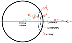
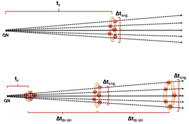
Figure A1: Left panel: Multiple (the primary, the secondary and the tertiary) chunks at a distance $d_{\rm c}$ (when they become collisionless) from a QN. The typical angular separation between adjacent chunks is $2/N_{\rm c}^{1/2}$ where $N_{\rm c}$ is the total number of chunks. Right panel: Radial repetition in our model due to Coulomb collisions once chunks electrons are trapped by the WI-saturated magnetic field (see §C). $t_{\rm c}=d_{\rm c}/c\sim 93$ years$\times m_{\rm c,22.3}^{1/5}/(\Gamma_{\rm c,2.5}^{1/5}n_{\rm amb.,-1}^{\rm ns\ 3/5})$ (see Eq. (A2)) is the time since the QN, in the NS frame, it takes the chunks to become collisionless. The total angular time delay between the primary chunk and the outmost chunk (within detector’s sensitivity) is $\Delta t_{\rm ang.}\sim N_{\rm c}^{\rm obs.}\times P_{\rm c,ang.}^{\rm obs.}$ where $N_{\rm c}^{\rm obs.}$ is the number of chunks within detector sensitivity and $P_{\rm c,ang.}^{\rm obs.}$ the average angular time separation between succesive chunks (see Eq.(A3)).

Appendix A Ejecta geometry, properties and angular periodicity

Figure A1 illustrates the geometry and distribution of chunks as seen by an observer. We assume a uniformly spaced chunks case here (see Appendix SA in Ouyed et al. 2021 for details and other geometries). For the simplest isotropic distribution of chunks around the center of the QN we have $N_{\rm c}\pi\Delta\theta_{\rm c}^{2}=4\pi$ with $\Delta\theta_{\rm c}\sim 2/N_{\rm c}^{1/2}$ the angular separation between adjacent chunks and $N_{\rm c}$ the total number of chunks. The number of chunks per ring of index $i_{\rm r}$ is $N(i_{\rm r})=2\pi(i_{\rm r}\Delta\theta_{\rm c})/\Delta\theta_{\rm c}=2\pi\times i_{\rm r}$ with $i_{\rm r}=0$ corresponding to the primary chunk so that $N(0)=1$. The total number of chunks up to ring $i_{\rm r,max.}$ is $N(i_{\rm r,max.})=\sum_{i=0}^{i_{r,max.}}N(i_{\rm r})=1+2\pi\sum_{i=1}^{i_{r,max.}}i_{\rm r}=1+2\pi\times\frac{i_{r,max.}(i_{r,max.}+1)}{2}=1+\pi\times i_{r,max.}(i_{r,max.}+1)$. Thus, there are roughly 1 primary, $2\pi\sim 6$ secondary and $4\pi\sim 12$ tertiary chunks adding up to a total of $(1+6\pi)\sim 19$ chunks. The details can be found in Appendix SA in Ouyed et al. (2021) where one can show that using the averaged viewing angle for the Primary (“P”), secondary (“S”) and tertiary (“T”) chunks one finds

$$f(\Gamma_{\rm c},\bar{\theta}_{\rm P}) \sim 1+0.18\frac{\Gamma_{\rm c,2.5}^{2}}{N_{\rm c,6}}$$ (A1)

$$f(\Gamma_{\rm c},\bar{\theta}_{\rm S}) \sim 1+0.97\frac{\Gamma_{\rm c,2.5}^{2}}{N_{\rm c,6}}$$

$$f(\Gamma_{\rm c},\bar{\theta}_{\rm T}) \sim 1+6.67\frac{\Gamma_{\rm c,2.5}^{2}}{N_{\rm c,6}}\ .$$

The average variation in $f(\Gamma_{\rm c},\theta_{\rm c})$ between successive chunks is $\Delta f\sim\frac{1.6}{\pi}\times\frac{\Gamma_{\rm c,2.5}^{2}}{N_{\rm c,6}}$ (Eq. (SA7) in Ouyed et al. 2021).

The time it takes a QN chunk to become collisionless as it travels in the ambient medium since the QN event is (see Eq. (SB13) and Appendix SB in Ouyed et al. 2021 for details)

$$t_{\rm c,ang.}^{\rm obs.}\simeq 6.0\ {\rm hrs}\times(1+z)f(\Gamma_{\rm c},\theta_{\rm c})\times\frac{m_{\rm c,22.5}^{1/5}}{\Gamma_{\rm c,2.5}^{11/5}n_{\rm amb,-1}^{3/5}}\ .$$ (A2)

In the NS frame it is $\Gamma_{\rm c}t_{\rm c,ang.}=\Gamma_{\rm c}t_{\rm c,ang.}^{\rm obs.}(1+z)/D(\Gamma_{\rm c},\theta_{\rm c})\sim 93\ {\rm years}\times m_{\rm c,22.3}^{1/5}/\Gamma_{\rm c,2.5}^{1/5}n_{\rm amb.,-1}^{\rm ns\ 3/5}$.

The average angular time separation between chunks, from $\Delta t_{\rm ang}^{\rm obs.}\propto\Delta f$, is then

$$P_{\rm c,ang.}^{\rm obs.}\simeq 3.0\ {\rm hrs}\times(1+z)\times\frac{m_{\rm c,22.5}^{1/5}}{N_{\rm c,6}\Gamma_{\rm c,2.5}^{1/5}n_{\rm amb,-1}^{3/5}}\ ,$$ (A3)

keeping in mind that $m_{\rm c}=\frac{E_{\rm QN}^{\rm ke}}{N_{\rm c}\Gamma_{\rm c}c^{2}}\sim 10^{22.3}\ {\rm gm}\times\frac{E_{\rm QN,52}^{\rm ke}}{N_{\rm c,6}\Gamma_{\rm c,2.5}}$. Here $E_{\rm QN}^{\rm ke}\simeq 10^{52}$ ergs is the kinetic energy of the QN ejecta which is a small percentage of the total (confinement and gravitational) binding energy released when converting all of the neutrons of a NS to quarks (see §1).

As the chunk propagates away from the QN and expands it eventually becomes ionized and collisionless when the electron Coulomb collision length inside the chunk is of the order of its radius (see Appendix SB in Ouyed et al. 2021). The distance travelled by a chunk (in the parent NS frame) until it becomes collisionless is $d_{\rm c}=c\Gamma_{\rm c}\times(D(\Gamma_{\rm c},\theta_{\rm c})t_{\rm c,ang.}^{\rm obs.}/(1+z))$. I.e.

$$d_{\rm c}^{\rm ns}\simeq 28.7\ {\rm pc}\times\Gamma_{\rm c,2.5}^{-1/5}m_{\rm c,22.3}^{1/5}n_{\rm amb.,-1}^{\rm ns\ -3/5}\ .$$ (A4)

The chunk’s number density, $n_{\rm c}$ and radius ($R_{\rm c}=(m_{\rm c}/\frac{4\pi}{3}n_{\rm c}m_{\rm H})^{1/3}$ with $m_{\rm H}$ the hydrogen mass) when it becomes collisionless were derived in Appendix SA in Ouyed et al. (2021):

$$n_{\rm c} \simeq 3.7\times 10^{3}\ {\rm cm}^{-3}\times m_{\rm c,22.3}^{1/10}\Gamma_{\rm c,2.5}^{12/5}{n_{\rm amb,-1}}^{6/5}$$ (A5)

$$R_{\rm c} \simeq 9.3\times 10^{13}\ {\rm cm}\times m_{\rm c,22.3}^{3/10}\Gamma_{\rm c,2.5}^{-4/5}{n_{\rm amb,-1}}^{-2/5}\ .$$

We take the proton hadronic cross-section to be $10^{-27}$ cm² and the chunk opacity $\kappa_{\rm c}=0.1$ cm² gm^-1 when deriving the equations above (see Ouyed et al. 2021).

The corresponding chunk’s angular size is

$$\frac{R_{\rm c}}{d_{\rm c}^{\rm ns}}\simeq 1.1\times 10^{-6}\times\Gamma_{\rm c,2.5}^{-3/5}m_{\rm c,22.3}^{1/10}n_{\rm amb.,-1}^{\rm ns\ 1/5}\ .$$ (A6)

The angular size above remains constant since the chunk stops expanding once it is collisionless. It is independent of the viewing angle (i.e. it is the same for any chunk from a given QN) and it is weakly independent on most parameters. Once collisionless, the chunk remains so (and stops expanding) since the mean-free-path of an external proton with respect to the chunk’s density always exceeds the chunk’s size. Once set, the density (and thus the plasma frequency) and the size $n_{\rm c}$ and $R_{\rm c}$ remains fixed as the chunk encounters different ionized media inside and outside its host.

Appendix B Coherent Synchrotron Emission (CSE) from the collisionless QN chunks

The interaction between the ambient plasma protons (the beam) and the chunk’s electrons (the background plasma) triggers the Buneman Instability (BI) with the generation of electrostatic waves inducing an anisotropy in the chunk’s electron population thermal velocity by increasing the electron velocity component along the direction of motion of the chunk; i.e. $v_{\perp}<v_{\parallel}$. This anisotropy in turns triggers the thermal Weibel Instability (WI) which induces cylindrical current filaments along the direction of motion of the chunk and the generation of the WI magnetic field which saturates when it is close to equipartition value $B_{\rm c,s}^{2}/8\pi\sim n_{\rm c}m_{\rm p}c^{2}$. The filament’s initial width (i.e. its transverse size at t=0) is set by the dominant electron-WI mode with wavelength $\lambda_{\rm F}(t=0)=\lambda_{\rm F,min.}=\beta_{\rm WI}^{1/2}\times c/\nu_{\rm p,e}$ where $\beta_{\rm WI}=v_{\perp}/v_{\parallel}<1$ the chunk’s thermal anisotropy parameter ($v_{\perp}$ and $v_{\parallel}$ are the electron’s speed in the direction perpendicular and parallel to the beam; see Ouyed et al. 2021 and references therein for details). Here, $2\pi\nu_{\rm p,e}=\sqrt{4\pi e^{2}n_{\rm c,e}/m_{\rm e}}\simeq 9\times 10^{3}\ {\rm Hz}\times n_{\rm c,0}^{1/2}$ is the chunk’s plasma frequency and $n_{\rm c}$ its number density with $n_{\rm c,e}=n_{\rm c}$; $m_{\rm e}$ and $e$ are the electron mass and charge, respectively.

In the non-linear regime of the WI, the WI filaments merge and grow in time as $\lambda_{\rm F}(t)=\lambda_{\rm F,min.}\times\left(1+\frac{t}{t_{\rm m-WI}}\right)^{\delta_{\rm m-WI}}$ with $\delta_{\rm m-WI}$ the filament merging index and $t_{\rm m-WI}=\sqrt{\frac{m_{\rm p}}{m_{\rm e}}}\times\frac{\zeta_{\rm m-WI}}{\nu_{\rm p,e}}$ the corresponding characteristic merging timescale (see Appendix SC3 and Eq. (SC11) in Ouyed et al. 2021). The filaments grow in size until they reach a maximum size $\lambda_{\rm F,max.}=c/\nu_{\rm p,e}$ set by the plasma skin depth.

Theoretical studies and Particle-In-Cell (PIC) simulations of the thermal WI instability suggests $\delta_{\rm m-WI}\sim 0.8$ and $\zeta_{\rm m-WI}$ in the tens of thousands. We adopt $\delta_{\rm m-WI}\sim 1.0$ and $\zeta_{\rm m-WI}=10^{5}$ as the fiducial values. Together, the WI-BI tandem converts a percentage ($\zeta_{\rm BI}$) of the chunk’s electrons’ kinetic energy to magnetic field energy and to accelerating the chunk’s electrons to relativistic speeds. These then cool and yield the CSE in our model (see Appendix SC in Ouyed et al. 2021).

B.1 Bunch properties

The electrons, that have been accelerated by the BI are often spatially bunched in form of phase space holes (Roberts & Berk 1967; Dieckmann & Bret 2007). Electron bunching occurs in the peripheral region around the filaments with bunch size $\lambda_{\rm b}=\delta_{\rm b}\lambda_{\rm F}$ where $\delta_{\rm b}<1$ (see details in section SD and Figure S3 in Ouyed et al. 2021). The number of electrons per bunch is $N_{\rm e,b}=(2\pi\lambda_{\rm F}\lambda_{\rm b})\times(2R_{\rm c})\times n_{\rm c}$. Because $\lambda_{\rm F,min.}=\beta_{\rm WI}^{1/2}/\nu_{\rm p,e}$ and $n_{\rm c}\propto\nu_{\rm p,e}^{2}$, the number of electrons per bunch is (see also §SD2 and Eq. (SD11) in Ouyed et al. (2021))

$$N_{\rm e,b}(t)\simeq 8.8\times 10^{29}\times\delta_{\rm b}\beta_{\rm WI}R_{\rm c,15}\times\left(1+\frac{t}{t_{\rm m-WI}}\right)^{2\delta_{\rm m-WI}}\ .$$ (B1)

The maximum total number of filaments ($N_{\rm b,T}=(R_{\rm c}/\lambda_{\rm F})^{2}$) decreases over time as

$$N_{\rm b,T}=9\times 10^{16}\times\frac{R_{\rm c,15}^{2}n_{\rm c,0}}{\beta_{\rm WI}}\times\left(1+\frac{t}{t_{\rm m-WI}}\right)^{-2\delta_{\rm m-WI}}\ .$$ (B2)

The exact number of filaments is hard to quantify but it is likely to be much less than the maximum value given above.

B.2 CSE frequency and duration

The relativistic electrons in the bunch emit coherently in the frequency range $\nu_{\rm p,e}\leq\nu_{\rm CSE}\leq\nu_{\rm CSE,p}(t)$ with the peak CSE frequency given as $\nu_{\rm CSE,p}(t)=c/\lambda_{\rm b}(t)$. The bunches grow in size with the merging WI current filaments which induces a decrease in the peak CSE frequency (and the narrowing of the emitting band) as

$$\nu_{\rm CSE,p}(t)=\frac{\nu_{\rm CSE,p,max.}}{\left(1+\frac{t}{t_{\rm m-WI}}\right)^{\delta_{\rm m-WI}}}\ .$$ (B3)

At $t=0$, before filament merging starts, a given bunch emits in the frequency range $\nu_{\rm p,e}\leq\nu_{\rm CSE}\leq\nu_{\rm CSE,p,max.}=\nu_{\rm p,e}/\delta_{\rm b}\beta_{\rm WI}^{1/2}$. I.e.

$$\frac{\nu_{\rm CSE,p,max.}}{\nu_{\rm p,e}}=\frac{1}{\delta_{\rm b}\beta_{\rm WI}^{1/2}}\ .$$ (B4)

The minimum CSE peak frequency is set by the maximum bunch size from merging $\lambda_{\rm b,max.}=\delta_{\rm b}\lambda_{\rm F,max.}$. This gives $\nu_{\rm CSE,p,min.}=c/\lambda_{\rm F,max.}=\nu_{\rm p,e}/\delta_{\rm b}$ so that

$$\frac{\nu_{\rm CSE,p,min.}}{\nu_{\rm p,e}}=\frac{1}{\delta_{\rm b}}\ .$$ (B5)

I.e. while the lower limit (i.e. the chunk’s plasma frequency) is constant for a given chunk, the CSE frequency band becomes narrower as the peak frequency slides down from $\nu_{\rm p,e}/\delta_{\rm b}\beta_{\rm WI}^{1/2}$ to $\nu_{\rm p,e}/\delta_{\rm b}$. The CSE duration is found by setting $\nu_{\rm CSE,p}(\Delta t_{\rm CSE})=\nu_{\rm CSE,p,min.}$,

$$\Delta t_{\rm CSE} =t_{\rm m-WI}\times\left(\left(\frac{\nu_{\rm CSE,p,max.}}{\nu_{\rm CSE,p,min.}}\right)^{1/\delta_{\rm m-WI}}-1\right)\ .$$ (B6)

which for $\delta_{\rm m-WI}=1$ means

$$\Delta t_{\rm CSE}=t_{\rm m-WI}\times\left(\frac{1}{\beta_{\rm WI}^{1/2}}-1\right)\ .$$ (B7)

Hereafter, we take $\delta_{\rm b}=1$ (i.e. $\lambda_{\rm b}=\lambda_{\rm F}$) so that $\nu_{\rm CSE,p,max.}=\nu_{\rm p,e}/\beta_{\rm WI}^{1/2}$ and ${\nu_{\rm CSE,p,min.}}=\nu_{\rm p,e}$.

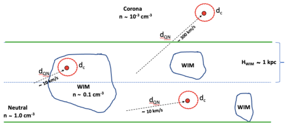
Figure B1: The birthplace and burst environment of QN chunks: This illustration showcases various scenarios involving different media both inside and outside a galaxy where a QN event can occur, leading to the transition of chunks into a collisionless state. Eventually, these chunks undergo the BI-WI instabilities, resulting in CSE bursts. During a QN event, millions of chunks are ejected, expanding radially away from the QN source. The resulting FRBs can be classified into three primary scenarios: (i) Halo-Born-Halo-Bursting chunks, which produce one-off FRBs; (ii) Disk-Born-Halo-Bursting chunks, which yield radially periodic FRBs; (iii) Disk-Born-Disk-Bursting chunks, leading to radial repeating FRBs. Angular repetition can occur in any of these three scenarios when peripheral chunks from the same QN event are detected.

B.3 CSE luminosity

For each ambient electron swept-up by the chunk, a fraction $\zeta_{\rm BI}$ of its kinetic energy is first converted by the BI into heat which is subsequently emitted as CSE by the chunk’s accelerated electrons (via the WI). The CSE luminosity is $L_{\rm CSE}=(\zeta_{\rm BI}\Gamma_{\rm c}m_{\rm e}c^{2})\times(\pi R_{\rm c}^{2}\Gamma_{\rm c}n_{\rm plasma}^{\rm ns}c)$. Or,

$$L_{\rm CSE}\simeq 6.2\times 10^{36}\ {\rm erg\ s}^{-1}\times\zeta_{\rm BI}\Gamma_{\rm 2.5}^{2/5}m_{\rm c,22.3}^{3/5}n_{\rm plasma,-1}^{\rm ns\ 1/5}\ ,$$ (B8)

where we made use of Eq. (1) and recall that here $n_{\rm amb.}^{\rm ns}$ is in the NS frame. The kinetic energy of the chunk converted to CSE emission is $E_{\rm CSE}=L_{\rm CSE}t_{\rm BI,s}$ with $t_{\rm BI,s}\simeq\frac{3}{2}(m_{\rm p}/m_{\rm e})^{1/3}/\nu_{\rm p,e}$ the BI saturation time (see Appendix SC in Ouyed et al. 2021). Thus

$$E_{\rm CSE}\simeq 1.1\times 10^{38}\ {\rm erg\ s}^{-1}\times\frac{\zeta_{\rm BI}\Gamma_{\rm 2.5}^{2/5}m_{\rm c,22.3}^{3/5}n_{\rm plasma,-1}^{\rm ns\ 1/5}}{\nu_{\rm p,e}}\ .$$ (B9)

We should point out that $n_{\rm amb.}^{\rm ns}$ here is the density of the ionized plasma the chunk is propagating in. This density may be different from that of the medium where the chunk first became collisionless and which sets and fixes the chunk’s intrinsic density $n_{\rm c}$ and thus its plasma frequency and related quantities. This is a fundamental difference as illustrated in Figure B1 but which has an impact only on the luminosity (i.e. the FRB fluence) during bursting. Hereafter we set $n_{\rm plasma}^{\rm ns}=n_{\rm amb.}^{\rm ns}$, effectively assuming that the bursting environment is the birth environment but one should keep in mind that if and when necessary one must multiply the CSE luminosity by $n_{\rm plasma}^{\rm ns}/n_{\rm amb.}^{\rm ns}$. With $n_{\rm plasma}^{\rm ns}=n_{\rm amb.}^{\rm ns}$ we can express $E_{\rm CSE}$ in terms of $\nu_{\rm p,e}$ via $n_{\rm amb.}^{\rm ns}\propto n_{\rm c}^{5/6}\propto\nu_{\rm p,e}^{5/3}$.

To summarize, the key equations (in the chunk’s frame) defining the CSE in our model are

$$\nu_{\rm CSE,p,min.} =\nu_{\rm p,e}$$ (B10)

$$\nu_{\rm CSE,p,max.} =\frac{\nu_{\rm p,e}}{\beta_{\rm WI}^{1/2}}$$

$$t_{\rm m-WI} =\sqrt{\frac{m_{\rm p}}{m_{\rm e}}}\times\frac{\zeta_{\rm m-WI}}{\nu_{\rm p,e}}$$

$$E_{\rm CSE} \simeq 1.4\times 10^{36}\ {\rm ergs}\times\frac{\zeta_{\rm BI}m_{\rm c,22.3}^{7/12}}{\nu_{\rm p,e}^{2/3}}\ ,$$

which all depend on the chunk’s plasma frequency $\nu_{\rm p,e}$. The CSE duration is given in Eq. (B7). Because $E_{\rm CSE}<<E_{\rm c}^{\rm ke}=\frac{m_{\rm e}}{m_{\rm p}}\times\Gamma_{\rm c}m_{\rm c}c^{2}$, a chunk can experience many CSE episodes during its lifetime (see Appendix C).

Appendix C Radial periodicity

Once the Weibel instability saturates, electrons will be trapped by the generated magnetic field. Coulomb collisions set-in and the dissipation of the magnetic field starts. Heating of electrons during filament merging ceases on the maximum filament size is reached at which point CSE cools electrons to $\sim$ 511 keV. The diffusive decay timescale of the WI-generated magnetic field can be estimated from $t_{\rm B,diff.}\sim\lambda_{\rm F,max.}^{2}/\eta_{\rm B}$ where $\lambda_{\rm F,max.}\sim c/\nu_{\rm p,e}$ is the filament’s maximum size and $\eta_{\rm B}=m_{\rm e}c^{2}\nu_{\rm coll.}/4\pi n_{\rm c,e}e^{2}=\nu_{\rm coll.}c^{2}/\nu_{\rm p,e}^{2}$ the diffusion coefficient with $n_{\rm c,e}=n_{\rm c}$ (e.g. Lang 1999). The electron Coulomb collision frequency is $\nu_{\rm coll.}=9.2\times 10^{-11}\ {\rm s}^{-1}\times n_{\rm c,0}\ln{\Lambda}/T_{\rm e,keV}^{3/2}$ where the electron temperature is in keV (e.g. Richardson 2019). A more rigorous assessment of the dissipation of the magnetic field requires simulations and is beyond the scope of this paper. However, it is reasonable to take the analytical value $t_{\rm B,diff.}\sim 1/\nu_{\rm coll.}$ as an order of magnitude estimate. A maximum dissipation timescale can be estimated by taking $T_{\rm e}=511$ keV and $\ln{\Lambda}=10$ to get $t_{\rm B,diff.}\sim 1.7\times 10^{6}\ {\rm years}/n_{\rm c,0}$. It is shorter if the electrons are cooled below 511 keV.

Once the magnetic field dissipates, another BI-WI is triggered and a new CSE episode starts as the chunk keeps propagating in the ambient plasma. In terms of the plasma frequency (with $n_{\rm c}\propto\nu_{\rm p,e}^{2}$), and in the observer’s frame, the corresponding period is $P_{\rm c,rad.}^{\rm obs.}=(1+z)t_{\rm B,diff.}/D(\Gamma_{\rm c},\theta_{\rm c})$. I.e.

$$P_{\rm c,rad.}^{\rm obs.}\sim 31.8\ {\rm days}\times\frac{1}{(1+z)f(\theta_{\rm c})}\times\frac{\Gamma_{\rm c,2.5}}{{\nu_{\rm p,e,9}^{\rm obs.}}^{2}}\sim 267.8\ {\rm days}\times(1+z)f(\theta_{\rm c})\times\frac{1}{\Gamma_{\rm c,2.5}^{17/5}m_{\rm c,22.3}^{1/10}n_{\rm amb.,-1}^{\rm ns\ 6/5}}\ .$$ (C1)

The distance travelled between successive BI-WI episodes, $d_{\rm c,rad.}^{\rm ns}=c\Gamma_{\rm c}t_{\rm B,diff.}$ (in the NS frame), is

$$d_{\rm c,rad.}^{\rm ns} \sim 28.7\ {\rm kpc}\times\frac{1}{\Gamma_{\rm c,2.5}^{7/5}m_{\rm c,22.3}^{1/10}n_{\rm amb.,-1}^{\rm ns\ 6/5}}\ .$$ (C2)

Periodic repetition would ensue if the length of the ambient plasma, $L_{\rm plasma}$ exceeds $d_{\rm c,rad.}$. This translates to

$$n_{\rm amb.}^{\rm ns}>n_{\rm amb.,c}^{\rm ns}\sim 0.31\ {\rm cm}^{-3}\times\frac{1}{L_{\rm Gal.,10{\rm kpc}}^{5/6}\Gamma_{\rm c,2.5}^{7/6}m_{\rm c,22.3}^{1/12}}\ ,$$ (C3)

which is very weakly dependent on the chunk’s mass $m_{\rm c}$. The higher the $n_{\rm c}$ the higher the plasma frequency (i.e. a higher Coulomb collision frequency) and thus the faster the magnetic dissipation timescale $\propto n_{\rm c}^{-1}$ which translates to shorter radial periods.

Appendix D The spectrum

In our model, the CSE spectrum from a given chunk is a convolution of the spectrum from a single bunch of size $\lambda_{\rm b}$ (with $\nu_{\rm p,e}<\nu_{\rm CSE}\leq\nu_{\rm CSE,p}(t)=\frac{c}{\lambda_{\rm b}(t)}$) and the distribution of bunch size $\lambda_{\rm b}$ within a given chunk. The distribution of bunch size and its evolution as the filaments merge remains to be determined. The temporal evolution of the convolved spectrum depends on the filament merging rate. I.e. as the filaments grow in size so does the peak of the distribution of bunch size which translates to the decrease in the overall maximum CSE frequency.

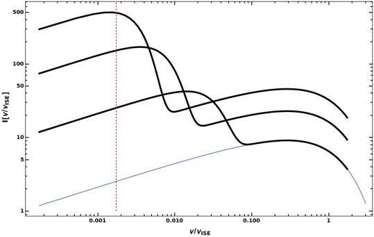
Figure D1: Normalized CSE spectrum: Normalized Intensity versus $\nu/\nu_{\rm ISE,p}$ with the incoherent synchrotron peak frequency $\nu_{\rm ISE,p}=\frac{3}{2}\gamma_{\rm e}^{2}\nu_{\rm B}$; $\nu_{\rm B}=\sqrt{\frac{m_{\rm p}}{m_{\rm e}}}\nu_{\rm p,e}$ in our model. The red vertical line shows the chunk’s plasma frequency $\zeta_{\rm p,e}=\nu_{\rm p,e}/\nu_{\rm ISE,p}=(\frac{3}{2}\gamma_{\rm e}^{2}\sqrt{\frac{m_{\rm p}}{m_{\rm e}}})^{-1}$. The bottom curve is the incoherent synchrotron spectrum in the $\nu_{\rm p,e}<\nu<\nu_{\rm CSE,p}$ frequency range from a single bunch containing $N_{\rm e}=20$ electrons and $\gamma_{\rm e}=3.0$ (see Eq. (D1)). The corresponding CSE spectrum with $(\nu_{\rm CSE,p},N_{\rm e})=(20\nu_{\rm p,e},10)$ is also shown which follows the $\nu^{1/3}$ of ISE curve at $\nu<\nu_{\rm CSE,p}$ and a steep exponential decay $e^{-(\nu_{\rm CSE,p})^{2}}$ for $\nu<\nu_{\rm CSE,p}$. The two top curves depict the time evolution of CSE from the bunch as it grow in size with $(\nu_{\rm CSE,p},N_{\rm e})=(5\nu_{\rm p,e},25)$ and $(2\nu_{\rm p,e},50)$, respectively. As the bunch grows in size, $\nu_{\rm CSE,p}=c/\lambda_{\rm b}$ decreases while the number of electrons $N_{\rm e}$ oncreases; see Appendix D for details.

D.1 A single bunch

We start with the incoherent synchrotron emission spectrum (ISE) for a single electron with Lorentz factor $\gamma_{\rm e}$ (e.g. Jackson (1999))

$$F(\zeta)=\frac{9}{\sqrt{3}{8\pi}}\zeta\int_{\zeta}^{\infty}K_{5/3}(x)dx\ ,$$ (D1)

with $\zeta=\nu/\nu_{\rm ISE,p}$ and $\nu_{\rm ISE,p}=\frac{3}{2}\gamma_{\rm e}^{2}\nu_{\rm c}$ the incoherent spectrum peak frequency while $\nu_{\rm c}$ is the cyclotron frequency. The $K_{5/3}$ is the modified Bessel function of second kind of order 5/3. Due to the magnetic field reaching near equipartition with the chunk’s protons at WI saturation we have $\nu_{\rm c}\sim\sqrt{\frac{m_{\rm p}}{m_{\rm e}}}\nu_{\rm p,e}$ . In these units, $\zeta_{\rm p,e}=\nu_{\rm p,e}/\nu_{\rm ISE}=(\frac{3}{2}\gamma_{\rm e}^{2}\sqrt{\frac{m_{\rm p}}{m_{\rm e}}})^{-1}$.

For simplicity, we assume a mono-energetic electron population per bunch. For a bunch which contains $N_{\rm e}$ electrons and which has a Gaussian distribution and r.m.s bunch length $\lambda_{\rm b}$ (with $\nu_{\rm CSE,p}=\frac{c}{\lambda_{\rm b}}$), the spectrum is (see Appendix SD in Ouyed et al. (2020) and references therein)

$$F_{\rm b}(\zeta,\zeta_{\rm CSE,p}(t))=F(\zeta)\times N_{\rm e}\left(1+(N_{\rm e}-1)e^{-\left(\frac{\zeta}{\zeta_{\rm CSE,p}(t)}\right)^{2}}\right)\ ,$$ (D2)

with $\zeta_{\rm CSE,p}(t)=\nu_{\rm CSE,p}(t)/\nu_{\rm ISE}$. Also, $\zeta_{\rm CSE,p,max.}=\zeta_{\rm p,e}/\beta_{\rm WI}^{1/2}$ and $\zeta_{\rm CSE,p,min.}=\zeta_{\rm p,e}$.

The $F(\zeta)\times N_{\rm e}$ term is the ISE intensity which scales linearly with $N_{\rm e}$ in the $\zeta_{\rm p,e}\leq\zeta\leq\zeta_{\rm ISE,p}$ frequency range. The CSE dominates when (using $N_{\rm e}-1\simeq N_{\rm e}$)

$$N_{\rm e}e^{-\left(\frac{\zeta}{\zeta_{\rm CSE,p}}\right)^{2}}>1\quad{\rm or}\quad\nu<\nu_{\rm CSE,p}\times\frac{\sqrt{\ln{N_{\rm e}}}}{2\pi}\sim\nu_{\rm CSE,p}\ ,$$ (D3)

with $N_{\rm e}$ given in Eq. (B1). I.e. for $\nu<\nu_{\rm CSE,p}$ the spectrum is the $N_{\rm e}F(\zeta)$ spectrum boosted in intensity by $N_{\rm e}$. The CSE follows the $\nu^{1/3}$ slope for $\nu<\nu_{\rm CSE,p}$ while it decays exponentially as $e^{-\left(\frac{\nu}{\nu_{\rm CSE,p}}\right)^{2}}$ for $\nu>\nu_{\rm CSE,p}$.

In Figure D1, we show an example of CSE spectrum for $\gamma_{\rm e}=3$ and three different time steps with $(\nu_{\rm CSE,p},N_{\rm e})=(20\nu_{\rm p,e},10)$, $(5\nu_{\rm p,e},25)$ and $(2\nu_{\rm p,e},50)$. Over time, the peak CSE frequency decreases (due to bunch size growth) as $\nu_{\rm CSE,p}\propto t^{-\delta_{\rm m-WI}}$ while the number of electrons in a bunch increases as $N_{\rm e}\propto t^{2\delta_{\rm m-WI}}$ boosting the CSE.

D.2 A distribution of bunches

Consider $N_{\rm b}$ bunches with a distribution in size $\lambda_{\rm b}$ and a corresponding $\nu_{\rm CSE,p}=c/\lambda_{\rm b}$ distribution $PDE(\nu_{\rm CSE,p})$ where ${\nu_{\rm CSE,p,min.}}=c/\lambda_{\rm b,min.}\leq\nu_{\rm CSE,p}\leq{\nu_{\rm CSE,p,max.}}^{\rm max.}=c/\lambda_{\rm b,max.}$. The cumulative CSE spectrum is then

$$F_{\rm cum.}(\zeta)=\int_{{\zeta_{\rm CSE,p,min.}}}^{{\zeta_{\rm CSE,p,max.}}}F_{\rm b}(\zeta,\zeta_{\rm CSE,p}){\rm PDE}(\zeta_{\rm CSE,p})d\zeta_{\rm CSE,p}\ .$$ (D4)

So far we ignored the turbulent nature of the filament merging during the WI and the intermittent acceleration of the chunk electrons. The final spectrum is much more complex than what is presented here and will be studied elsewhere.

References

- Achterberg et al. (2007) Achterberg, A., Wiersma, J. & Norman, C. A. 2007, A&A 475, 19
- Amiri et al. (2021) Amiri, M., Andersen, B. C., Bandura, K. et al. 2021, ApJSupplement, 257, 59
- Andersen et al. (2023) Andersen, B. C., Kevin Bandura,K., Bhardwaj, B. et al. ApJ, 947, 83
- Bannister et al. (2019) Bannister, K. W., et al. (2019). ”The Detection of an Extremely Bright Fast Radio Burst in a Phased Array Feed Survey.” The Astrophysical Journal, 870(2), 114.
- Bera & Chengalur (2019) Bera A., & Chengalur J. N. 2019, MNRAS, 490, L12
- Bhandari et al. (2002) Bhandari, S., Heintz, K. E., Aggarwal, K., et al. 2022, AJ, 163, 69
- Chatterjee et al. (2017) Chatterjee, S., Law, C. J., Wharton, R. S., et al. 2017, Nature, 541, 58
- CHIME/FRB Collaboration et al. (2021) CHIME/FRB Collaboration and Amiri, M. et al. 2021, ApJS, 257, 59
- CHIME/FRB Collaboration et al. (2023) CHIME/FRB Collaboration and Amiri, M. et al. 2023 [arXiv:2311.00111]
- Connor et al. (2016) Connor, L., Jonathan Sievers,J. & Ue-Li 2016, MNRAS, 458, L19
- Cordes et al. (2016) Cordes, J. M., Wharton, R. S., Spitler, L. G. et al. 2016, preprint (arXiv:1605.05890)
- Cordes & Chatterjee (2019) Cordes, J. M., & Chatterjee, S. (2019). ”Fast Radio Bursts: An Extragalactic Enigma.” Annual Review of Astronomy and Astrophysics, 57, 417
- Cordes & Chatterjee (2021) Cordes, J. M., et al. (2021). ”Fast Radio Burst Extragalactic Dispersion and Rotation Measure Simulations.” The Astrophysical Journal, 913(2), 151
- Day et al. (2020) Day, C. K., Deller, A. T., Shannon, R. M., et al. 2020, MNRAS, 497, 3335
- Dieckmann & Bret (2007) Dieckmann, M. E., Bret, A. & Shukla P. K. 2007, Plasma Phys. Controll. Fusion, 49, 1989
- Faucher-Giguère & Kaspi (2006) Faucher-Giguère, C.-A., & Kaspi, V. M. 2006, ApJ, 643, 332
- Ferreire (2001) Ferreire, K. 2001, Review of Modern Physics, 73, 1031
- Fronsecra et al. (2020) Fonseca E., et al., 2020, ApJ, 891, L6
- Gajjar et al. (2018) Gajjar, V. et al. 2018, ApJ, 863, 2
- Gerin et al. (2015) Gerin, M., Ruaud, M., Goicoechea, J. R., et al. 2015, A&A, 573, A30
- Gopinath et al. (2023) Gopinath, A., Bassa, C. G., Pleunis, Z. et al. 2023, ?? [arXiv:2305.06393]
- Haffner et al. (2009) Haffner, L. M., Dettmar, R.-J., Beckman, J. E., et al. 2009, Rev. Mod. Phys., 81, 969
- Hoyle & Ellis (1963) Hoyle, F., & Ellis, G. R. A. 1963, Aust. J. Phys., 16, 1
- Jackson (1999) Jackson, J. D., Classical Electrodynamics, 3rd ed. (Wiley, New York, 1999)
- Kaspi & Beloborodov (2017) Kaspi V. M., & Beloborodov A. M. 2017, ARA&A, 55, 261
- Kumar et al. (2021) Kumar, P., Shannon, R. M., Flynn, C. 2021, MNRAS, 500, 2525
- Lang (1999) Lang, K. R. 1999, Astrophysical Formulae, Third Edition (New York: Springer)
- Li & Zanazzi (2021) Li D. & Zanazzi J. J. 2021, ApJ, 909, L25
- Loeb et al. (2014) Loeb, A., Shvartzvald, Y. & Maoz, D. 2014, MNRAS, 439, L46
- Lorimer et al. (2007) Lorimer, D. R., et al. 2007, Science, 318, 777
- Lyutikov et al. (2020) Lyutikov M., Barkov M. V., Giannios D., 2020, ApJ, 893, L39
- Macquart & Ekers (2018) Macquart, J. P., & Ekers, R. D. 2018, MNRAS, 474, 1900
- Macquart et al. (2020) Macquart, J.-P., Prochaska, J. X., McQuinn, M., et al. 2020, Nature, 581, 391
- Mannings et al. (2021) Mannings, A. G., Fong, W.-f., Simha, S., et al. 2021, ApJ, 917, 75
- Marcote et al. (2020) Marcote, B., Nimmo, K., Hessels, J.W.T. et al. 2020, Nature 577, 190
- Masui et al. (2015) Masui K., et al., 2015, Nature, 528, 523
- Mckinven et al. (2023) Mckinven, R., Gaensler, B. M., Michilli, D., et al. 2023, ApJ, 951
- Metzger et al. (2019) Metzger, B. D., et al. (2019). ”Fast Radio Bursts as Probes of Extragalactic Magnetic Fields.” Monthly Notices of the Royal Astronomical Society, 485(3), 4091
- Ouyed & Leahy (2009) Ouyed, R., & Leahy, D. 2009, ApJ, 696, 562
- Ouyed et al. (2017a) Ouyed, R., Leahy, D., Koning, N. & Shand, Z. 2017a, “Quark-nova compact remnants: Observational signatures in astronomical data and implications to compact stars”. Proceedings of the Fourteenth Marcel Grossmann Meeting, pp. 3387-3391, DOI: https://doi.org/10.1142/9789813226609-0435 [arXiv:1601.04236]
- Ouyed et al. (2017b) Ouyed, R., Leahy, D., Koning, N. & Staff, J. E. 2017b, “Quark-Novae in binaries: Observational signatures and implications to astrophysics”. Proceedings of the Fourteenth Marcel Grossmann Meeting, pp. 1877-1882, DOI: https://doi.org/10.1142/9789813226609-0197 [arXiv:1601.04235]
- Ouyed et al. (2020) Ouyed, R., Leahy, D. & Koning, N. 2020, Research in Astronomy and Astrophysics, 20, 27
- Ouyed et al. (2021) Ouyed, R., Leahy, D. & Koning, N. 2021, MNRAS, 500, 4414
- Ouyed (2022a) Ouyed,, R. 2022a, “The Micro-physics of the Quark-nova: Recent Developments”. Astrophysics in the XXI Century with Compact Stars [eISBN 978-981-12-2094-4], 53-83
- Ouyed (2022b) Ouyed,, R. 2022b, Universe. 8, 322
- Pastor-Marazuela et al. (2021) Pastor-Marazuela, I., Connor, L., van Leeuwen, J. 2021, Nature, 596, 7873
- Pearlman et al. (2020) Pearlman, A. B. et al. 2020, ApJ, 905, L27
- Persson et al. (2014) Persson, C. M., Gerin, M., Mookerjea, B., et al. 2014, A&A, 568, A37
- Petroff et al. (2019) Petroff, E., Hessels, J. W. T. & Lorimer, D. R. 2019, A&A Rev., 27, 4
- Petroff et al. (2022) Petroff, E., Hessels, J. W. T. & Lorimer, D. R. 2022, A&A Rev., 30, 2
- Platts et al. (2019) Platts E., Weltman A., Walters A. et al. 2019, Phys. Rep., 821, 1
- Pleunis et al. (2020) Pleunis, Z., Good, D. C., Kaspi, V. M., et al. 2021, ApJ, 923, 1
- Pleunis et al. (2021) Pleunis, Z., Michilli, D., Bassa, C. G. et al. 2021, ApJ, 911, L3
- Prochaska et al. (2019a) Prochaska, J. X., et al. 2019a, MNRAS, 485, 648
- Prochaska et al. (2019b) Prochaska, J. X., et al. 2019b, ApJ, 887, 13
- Rane et al. (202) Rane, A., et al. 2020, Nature, 587, 63
- Reynolds (1991) Reynolds, R. J. 1991, in The Interstellar Disk-Halo Connection in Galaxies, ed. H. Bloemen, 144, 67
- Richardson (2019) Richardson, A. S. 2019, NRL Plasma Formulary (Naval Research Lab Washington, DC, Pulsed Power Physics Branch)
- Roberts & Berk (1967) Roberts, K. V. & Berk, H. L. 1967, Phys. Rev. Lett., 19, 297
- Ryder et al. (2023) Ryder, S. D., Bannister, K. W., Bhandari, S. et al. 2023, Science, 382, 294
- Sand et al. (2022) Sand, K. R., Faber, J. T., Gajjar, V. et al. 2022, ApJ, 932, 98
- Simha et al. (2023) Simha, S., Lee, K.-G., Prochaska, J. X. et al. 2023 [arxiv: 2303.07387v1]
- Snelders et al. (2023) Snelders, M. P., Nimmo, K., Hessels, J. W. 2023, Nature Astronomy, 7, 1486
- Spanakis-Misirlis (2021) Spanakis-Misirlis, A. 2021, https://ascl.net/2106.028 [ascl:2106.028]
- Spitler et al. (2014) Spitler, L. G., Cordes, J. M., Hessels, J. W. T., et al. 2014, ApJ, 790, 101
- Spitler et al. (2016) Spitler L. G., et al., 2016, Nature, 531, 202
- Staff, et al. (2006) Staff, J. E., Ouyed, R. & Jaikumar, P. 2006, ApJ, 645, L145
- Taylor & Cordes (1993) Taylor, J. H. & Cordes, J. M. 1993, ApJ, 411, 674
- Tendulkar et al. (2021) Tendulkar, S. P., Gil de Paz, A., Kirichenko, A. U. 2021, ApJ, 908, L12
- Thornton et al. (2013) Thornton, D., Stappers, B., Bailes, M., et al. 2013, Science, 341, 53
- Weber (2005) Weber, F. 2005, Progress in Particle and Nuclear Physics, 54, 193
- Yang & Zhang (2016) Yang, Y.-P. & Zhang, B. 2016, ApJ, 880, L31
- Yang et al. (2017) Yang, Y.-P., Luo, R., Li, Z. & Zhang, B. 2017, ApJ, 839, L25
- Zhang (2023) Zhang, B. 2023, Reviews of Modern Physics, 95, 035005