Neural Network Emulator for Atmospheric Chemical ODE

Abstract

Modeling atmospheric chemistry is complex and computationally intense. Given the recent success of Deep neural networks in digital signal processing, we propose a Neural Network Emulator for fast chemical concentration modeling. We consider atmospheric chemistry as a time-dependent Ordinary Differential Equation. To extract the hidden correlations between initial states and future time evolution, we propose ChemNNE , an Attention based Neural Network Emulator (NNE) that can model the atmospheric chemistry as a neural ODE process. To efficiently simulate the chemical changes, we propose the sinusoidal time embedding to estimate the oscillating tendency over time. More importantly, we use the Fourier neural operator to model the ODE process for efficient computation. We also propose three physical-informed losses to supervise the training optimization. To evaluate our model, we propose a large-scale chemical dataset that can be used for neural network training and evaluation. The extensive experiments show that our approach achieves state-of-the-art performance in modeling accuracy and computational speed.

[a]organization=School of Engineering Science, Lappeenranta-Lahti University of Technology LUT, city=Lahti, postcode=15110, country=Finland

[b]organization=Atmospheric Modelling Centre Lahti, Lahti University Campus, city=Lahti, postcode=15140, country=Finland

[c]organization=Institute for Atmospheric and Earth System Research (INAR), The University of Helsinki, city=Helsinki, postcode=00014, country=Finland

1 Introduction

In the past decades, deep learning has been proven as an efficient data-driven modeling approach that can handle large-scale datasets for complex digital signal processing, like images (Ramesh et al. (2021); Xu et al. (2023)), videos (Sauer et al. (2023)), audio (Radford et al. (2023)), and languages (Solaiman et al. (2019); OpenAI and et al. (2023); Touvron et al. (2023a, b)). It is intriguing to see if it can benefit chemical modeling problems. There are a number of approaches that use deep neural networks to resolve specific chemical problems, like Su et al. (2024); Goswami et al. (2024). In general, we can take the time evolution of the chemical compound concentration as an Ordinary Differential Equation (ODE), which can be modeled by the neural networks. The hidden chemical reactions are implicitly learned and optimized by training data. In such a way, we can build the neural networks as a surrogate model that can replace the numerical simulation for fast computation. Similar research works have been done in Wu et al. (2023); Ren et al. (2023). However, few studies have been conducted on large-scale atmospheric chemistry modeling or multiple-input-and-multiple-output chemical prediction. Therefore, in this study, we aim at an end-to-end efficient neural network that can model multiple chemical concentrations (49$\sim$300 aerosol chemical compounds) over time (one hour). Specifically, given the environmental parameters and initial chemical concentrations, not only it can predict the future states of the input chemical compounds, but it also predicts new chemicals generated in the process. We analyze the model performance by the concentration changes along the time by mean squared errors and running time. To interpret the learning ability of attention, we also analyze the key chemical components for their effects and correlations to other compounds. To the best of our knowledge, we propose the largest chemical concentration dataset that can be used for model training. Our proposed ChemNNE is also the first work using neural networks for atmospheric chemical emulators. To summarize, our contributions are:

• we propose the first neural network emulator for atmospherical chemical modeling. It can take the initial chemical concentration and environmental parameters as input, to predict the future evoluations.

• To model the inter- and intra-correlations among chemical data, we propose to use time-embedded attention to model the molecule concentration as a learnable time-dependent process.

• We propose to combine Fourier Neural Operator (FNO) and attention to model the signal in the spatial and frequency domain so that a fast neural ODE can be achieved for fast computation.

• To better constrain the chemical process, we propose physical-informed losses, including identity loss, derivative loss and mass conservation loss to ensure that the model can predict further future steps without violating the chemistry.

• We conduct extensive experiments on three large-scale tasks, including interperiod, intraperiod and hybridperiod tasks, to show the efficiency of our ChemNNE on various atmospheric chemical problems.

2 Related Work

In atmospheric chemistry, one important aspect is to study the oxidation of volatile organic compounds. With prior knowledge of the emitted chemical compounds and the main atmospheric reaction paths, researchers analyze and discover atmospheric phenomena from a micro view, i.e., the concentrations of very low volatile organic compounds (ppt or ppb range), or a macro view, i.e., cloud generation and air pollution through the formation and growth of atmospheric particles. From the mathematical perspective, we study the problem as a time-series problem or partial differential equation (PDE) problem. Given the booming development of deep learning, we will discuss deep learning based chemical modeling in the following sections.

2.1 Deep learning for chemical modeling

The rise of deep learning in the early 2010s has significantly expanded the scope of scientific discovery processes. Benefiting from the graphic processing units and coupled with new algorithms, deep learning or artificial intelligence has proved to be helpful in integrating scientific knowledge to solve diverse tasks across different domains. AI for chemistry, one of the promising research directions, has recently attracted a lot of researchers for investigation, like molecular design, materials (Volk et al. (2023); Goodall and Lee (2020)), physics (Hayat et al. (2020); Portillo et al. (2020)), atmosphere (Bassetti et al. (2023); Boiko et al. (2023); Castruccio et al. (2014)) and climate (Lam and et al. (2023); Bodnar et al. (2024); Bi et al. (2023)), and so on. For example, Volk et al. (2023) proposes to use a reinforcement learning system for multi-step nanoparticle chemistry, which can automatically explore the core-shell semiconductor particles for a self-driven fluidic laboratory. Abramson et al. (2024) propose Alphafold3 for protein structure prediction, which uses a very large-scale Protein Data Bank (PDB) to train a diffusion-based neural network for accommodating arbitrary chemical components. Chithrananda et al. (2020) propose to utilize the pre-trained transformers to discover the molecular property, offering competitive performance on drug design and other molecular predictions. Hayat et al. (2020) proposes a conservative learning framework on multi-band galaxy photometry to learn image representation. Without or with very few labels, it can achieve comparable or even better performance than the supervised approaches. To extract information from galaxy spectra, Portillo et al. (2020) propose a variational autoencoder (VAE) to reduce the dimensionality for latent space spectra interpolation and outlier detection. Graphcast (Lam and et al. (2023)) is one of the promising weather forecasting AI models that uses a graph neural network to predict the global weather with medium-range resolution. Recently, Aurora has revolutionized many facets of climate studies by leveraging vast amounts of data and proposing a foundation model with 1.3B parameters, achieving state-of-the-art performance in weather forecasting. Different from weather prediction models, atmospheric chemical models study the micro and macro chemical dynamics with physical constraints. It can be very useful for extreme weather study, air pollution prevention and so on. Bassetti et al. Bassetti et al. (2023) propose a conditional emulator via the conditional diffusion model to understand the impact of human actions on the earth system. Fine-tuned from the large language models (OpenAI and et al. (2023)), ChemGPT (Boiko et al. (2023)) is proposed to assist in autonomous chemical design and analysis, like reaction optimization and experimental automation.

2.2 Learning time series for natural science

Given the initial chemical compound concentration and environmental parameters, we can model the overall process as a time series problem. To solve time series, there are two major categories: 1) autoregression and 2) ODE process. Scientific hypotheses often take the form of discrete objects, such as symbolic formulas in physics or chemical compounds in pharmaceuticals and atmospheres. A differentiable space can be used for efficient optimization as it is amendable to gradient-based methods. For autoregression, RNN (Hochreiter and Schmidhuber. (1997)) and attention (Vaswani et al. (2017)) are two major approaches for temporal modeling. The RNN-based methods utilize the recurrent structure and capture temporal variations implicitly via time-dependent state transitions. On the other hand, attention, or transformer-based approaches discover the global temporal dependencies to determine which time step needs to be attended more for future prediction. Specifically, Li et al. (2019); Zhou et al. (2021) are two efficient self-attention models that can achieve remarkable performance on forecasting. Wu et al. (2021) present Autoformer that computes the auto-correlations among the time series data via Fast Fourier Transform. FEDformer (Zhou et al. (2022)) further improves it by utilizing the mixture-of-expert design to ensemble the specific knowledge learned from the frequency domain. Knowing partial time series data, TimeNet proposes the TimesBlock to project the 1D data to the 2D space and discover the inter- and intra-time correlations for forecasting.

The ODE/PDE process is another efficient approach that can explicitly model the neural network as a partial differential process for optimization. The advent of neural ODEs (Chen et al. (2018)) has opened new possibilities for novel ODE solver methods in physics (Hayat et al. (2020); Portillo et al. (2020)), chemistry (Jiang et al. (2020); Su et al. (2024); Goswami et al. (2024)), biology (Lu et al. (2021); Pokkunuru et al. (2023)) and so on. There exist three primary branches of deep learning based ODE process: 1) continuous learning (Raissi et al. (2019, 2020); Geneva and Zabaras (2020); Norcliffe et al. (2020)), 2) discrete learning (Zhu et al. (2019); Bhatnagar et al. (2019); Khoo et al. (2020); Biloš et al. (2021); Massaroli et al. (2020); Yildiz et al. (2019)), and 3) neural operators (Li et al. (2020); K. et al. (2024); Li et al. (2023, 2020)). The continuous learning utilizes NNs as a domain projector that maps the data to the continuous latent space for capturing global solution patterns. The idea is to embed the physics-informed losses into the training process to ensure that the behaviors of the network follow the ODE process. The discrete learning models the nonlinear dynamics on mesh grids by leveraging convolutional or graph NNs. Neural operators treat the mapping from initial conditions to solutions at time t as an input-output supervised task, which can be learned by neural operations. For example, Fourier Neural Opeartor (Li et al. (2020)) parameterizes the integral kernel directly in Fourier space as simple multiplication, which is a significant computation reduction. Spherical Fourier Neural Opeartor (Bonev et al. (2023)) generalizes the Fourier Transform as a spherical geometry, achieving stable autoregressive on long-term forecasting. The recent advance of Implicit Neural Representations (INR) shows potential to be used for predicting the spatially continuous solution of an ODE/PDE given a spatial position query. In this work, we will study this method and combine it with existing ODE methods for further improvements.

3 Method

3.1 Data preparation

The data set used to study atmospheric chemistry is modeled by ARCA box (Clusius et al. (2022)), which is a comprehensive toolbox for modeling atmospheric chemistry and aerosol processes. The model can be set up to any kinetic chemistry system, but most often the base chemistry scheme comes from the Master Chemical Mechanism (Jenkin et al. (2015, 1997); Saunders et al. (2003)). We used a subset of the MCM, augmented with the Peroxy Radical Autoxidation Mechanism (Roldin et al. (2019)), which simulates monoterpene autoxidation, crucial in producing low volatility vapors from biogenic volatile organic carbon (BVOC) emissions. The subset was selected so that it contains both biogenically and anthropogenically emitted compounds such as isoprene, monoterpenes, aromatics, alkenes and alkynes, and together with their reaction products contains altogether 3301 compounds and 9530 reactions. The kinetic chemistry system is converted to a system of ODEs using the Kinetic PreProcessor (Sandu et al. (2023)), and then incorporated in ARCA box and solved numerically to simulate the time series of the reaction products.

To create the dataset, we varied the initial concentrations of 49 precursors and three environmental conditions: temperature, relative humidity and short-wave radiation, affecting the reaction rates and photochemistry. Chemically related compounds were linked together and varied in tandem, resulting in 15 independently varied initial concentrations. To create the test data set the initial concentrations and environmental variables were either at their realistic upper and lower bounds, and additionally simulations where the environmental variables were in the middle values. This produced $2^{15}\times 3^{3}=884736$ different time series of the 3301 chemical compounds.

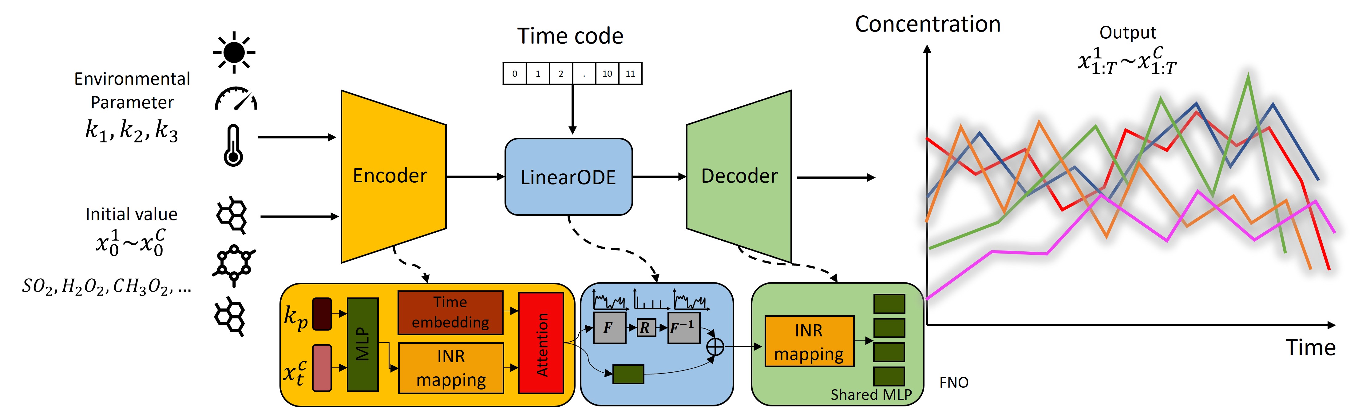
Figure 1: The proposed ChemNNE for chemical concentration prediction. It takes the environmental parameters and chemical initial concentration to predict the future chemical reaction process.

3.2 ChemNNE for Atmospheric modeling

To model the atmospheric chemical reaction, we propose the following framework in Figure 1. It consists of three parts: 1) encoder, 2) linearODE, and 3) decoder. Let us denote the initial chemical concentration as $x_{0}\in\mathbb{R}^{N}$, where $N$ is the number of chemical elements, and the environmental parameters as $k\in\mathbb{R}^{O}$, where $O$ is the number of environmental factors, e.g., temperature, humidity and radiation. Mathematically, given the time steps $t_{i}=0,1,...,T$, the proposed ChemNNE learns a linear ODE function that predicts time-dependent output chemical values $x_{t}\in\mathbb{R}^{N}$ as,

$$x_{t}=\psi\left(\varphi(x_{0},k)+\int_{[t_{0},t_{T}]}f(z(t))dt\right),\ \text{where}\ f(z(t))=\frac{dz(t)}{dt}$$ (1)

In Eq 1, it comprises three components: an encoder $\varphi$, the linearODE $f$, and a decoder $\psi$. The dynamics of the chemical process are characterized as $z(t)$. Given initial chemical concentration $x_{0}$, we have the latent space initial state $z_{0}=\varphi(x_{0},k)$, which serves as the initial condition for the ODE. The integral operation is evaluated by the proposed linearODE, which is achieved by the Fourier Neural Operation process. The Encoder is made of INR and time-dependent attention modules for extracting hidden correlations among different chemical components, and the decoder uses the shared MLP layers and INR module again for time prediction.

3.2.1 Time embedding and Implicit Neural Representation (INR) mapping

Observing the chemical reaction simulation, we can see that the chemical compounds usually dynamically change their concentrations over time. This oscillating behavior can resonate with radio frequency modulation, where the true signal can be encoded to the carrier wave by either changing its frequency or amplitude. As pointed out by Sitzmann et al. (2020), using neural networks for continuous and differentiable physical signals is challenging because the neural networks tend to oversmooth the high-frequency details and do not represent the derivatives of a target signal well. To introduce a differentiable time representation, we propose to use sinusoidal time embedding (Mildenhall et al. (2020)) to the time code, which can be described as follows.

$$\lambda(t)=F_{\Theta}\circ t=\left(sin(2\Theta\pi t),cos(2\Theta\pi t)\right)$$ (2)

Mathematically, given the time steps $t_{i}=0,1,...,T$, we project them onto a higher dimensional space $\mathbb{R}^{2L}$, where $F_{\Theta}\in\mathbb{R}^{L}$ is the L-length learnable parameters that can define the frequency of the time code. We represent the time as a combination of sine and cosine operators so that the network can learn to adjust the reaction frequency.

To obtain implicit neural representation (INR), we apply sine as a periodic activation function to the chemical input and hidden features, $x_{i}\rightarrow\phi_{i}(x_{i})=sin(W_{i}x_{i}+b),\text{where\ }W_{i}\sim\mathcal{U}(-6/\sqrt{(}N),6/\sqrt{(}N)),c\in\mathbb{R}$, as they are continuous changes in the physical world and it is memory efficient to compute the derivatives in the sine space without being constrained by discrete data samples. The initialized weight parameters ensure that the input to each sine activation is normally distributed with a standard deviation of 1. Physically, we can interpret the weights of the INR function as angular frequencies while the biases are phase offsets. Applying the sine function keeps signal amplitude constant while expanding frequency bands for high-frequency modeling.

3.2.2 Attention for chemical representation

Attention has been widely used in image, video, and language processing. Its success comes from its efficient nonlocal feature representation. For chemical modeling, we also expect an efficient approach that can model the long-term time evolution, so that similar chemical behavior across time or different chemical compounds can be utilized for pattern matching. In order to achieve that, we propose a time-dependent attention module, which can encode and decode the chemical data to the latent space for implicit neural representation. Mathematically, we can define the process as,

$$z_{\lambda}(t)=z_{\lambda}(t)+\text{ffn}\left(z_{\lambda}(t)+\sigma\left(\frac{Q_{z}K_{z}^{T}}{\sqrt{(}d)}\right)V_{z}\right)$$ (3)

where $z_{\lambda}(t)=sin\left[W(z_{0})+b\right]+\lambda(t)$, $Q_{z}=z_{\lambda}(t)W_{Q}$, $K_{z}=z_{\lambda}(t)W_{K}$, and $V_{z}=z_{\lambda}(t)W_{V}$. The $W_{*}$ is the learnable parameter. $z_{0}$ is the output feature of the INR mapping layer. As depicted in Figure 1, given the latent space chemical features, we apply the INR mapping first. Then we use the attention module to learn the nonlocal correlations. A feedforward network (ffn) is used to learn the residues for network update. Note that the activation of ffn is also a sine function to preserve the periodic behavior of chemical reactions.

3.2.3 Fourier Neural Operator (FNO)

To explore the derivatives of the chemical reactions, introducing ODE in the neural network can preserve the underlying physical laws. In recent works Chen et al. (2018); Li et al. (2023, 2020), neuralODE, like Torchdiffeq (Chen et al. (2018)), has been used for GPU based ODE approximation. However, the disadvantage is that it is not numerically stable and rather slow in computation. We propose to further simplify the ODE process as a Neural Fourier Operation. Given the continuous time representation, we use Fourier Transformation to project the signal to the frequency domain and learn the parametric partial differentiation process.

$$\begin{matrix}\!\begin{aligned} &z_{t+1}=\gamma\left(Wz_{t}+\mathcal{F}^{-1}(R_{\phi}\cdot(\mathcal{F}z_{t}))\right)\\ &(R_{\phi}\cdot(\mathcal{F}z_{t}))=\sum_{j=1}^{d_{v}}R_{k,l,j}{\mathcal{F}z_{t}}_{k,j},k=1,...,k_{max},j=1,...,d_{v}\end{aligned}\end{matrix}$$ (4)

We lift the signal to the frequency domain, given k frequency modes, we have $\mathcal{F}z_{t}(k)\in\mathbb{C}^{d_{v}}$ and $R_{\phi}(k)\in\mathbb{C}^{d_{v}\times d_{v}}$. $\gamma$ is the nonlinear activation. We define $R_{\phi}(k)$ as the truncation function that only keeps the maximal number of modes $k_{max}=|{k\in\mathbb{Z}_{d}:|k_{j}|\leq k_{max,j},forj=1,...,d}|$.

The advantages of using FNO for ODE computation are 1) it is faster to use Fourier Transform than convolution, as it is quasilinear, where the full standard integration of n points has complexity $O(n^{2})$; 2) the input and outputs of PDEs are continuous functions, so it is efficient to represent them in the Frequency domain for global convolution. In the experiments, we would show the complexity comparisons to demonstrate the efficiency of FNO.

3.2.4 Physical-informed losses.

To train the whole ChemNNE , not only do we utilize the commonly used Mean Squared Errors (MSE) between prediction and ground truth, but we also propose to utilize the first- and second-order derivation, and total mass conservation loss. Mathematically, we can define the overall losses as

$$Loss=\alpha_{1}L_{recon}+\alpha_{2}L_{d1}+\alpha_{3}L_{d2}+\alpha_{4}L_{idn}+\alpha_{5}L_{mass}$$ (5)

In Eq 5, $\alpha_{1}$ to $\alpha_{5}$ are the weighting parameters that balance all five loss terms. $L_{recon}$ is the reconstruction loss measures the discrepancy between the prediction and ground truth as $L_{recon}=|x(t)-x^{\prime}(t)|^{2}$. The first-order gradient loss enforces the predicted trajectories to closely follow the ground truth over time as $L_{d1}=|\frac{dx(t)}{dt}-\frac{dx^{\prime}(t)}{dt}|^{2}$. Similarly, we can define the second-order gradient loss as $L_{d2}=|\frac{dx^{2}(t)}{dt^{2}}-\frac{dx^{\prime 2}(t)}{dt^{2}}|^{2}$. Meanwhile, we can also enforce that the ChemNNE should preserve the initial condition unchanged during the training process. Hence we can define the identity loss as $L_{idn}=|x(t_{0})-\psi(\varphi(x(t_{0})))|^{2}$. Finally, we define the total mass conservation loss, ensuring that the mass of the predicted trajectory aligns with the mass of the ground truth at each time step. We have $L_{mass}=|\phi(x(t))-\phi(x^{\prime}(t))|^{2}$, where $\phi$ is the summation of all chemical components.

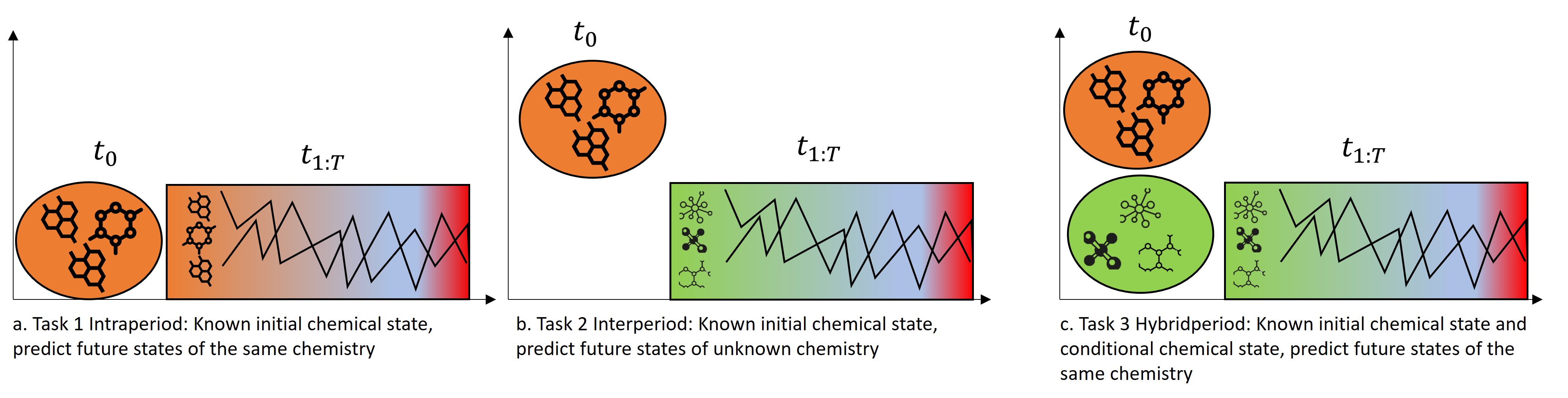
Figure 2: Three chemical prediction task for model evaluation.

Tasks	Training	Validation	Testing	Environment input	Chemical input	Chemical output
Task 1	88471	29485	29485	3	48	48
Task 2	176941	58987	58987	3	100	100
Task 3	265418	88471	88471	3	100	400

Table 1: Data summary of three tasks.

3.2.5 Evaluation

To compare the estimations of the proposed ChemNNE against others, we apply the mean absolute errors (MAE) and the root mean squared errors (RMSE) to express the average difference. We also use the mean bias error (MBE) to calculate the estimation bias. The analytic equations for the estimation are:

$$\begin{matrix}\!\begin{aligned} &MAE=\sum_{i=1}^{N}\frac{|X_{i}-Y_{i}|}{N}\\ &RMSE=\sqrt{\sum_{i=1}^{N}\frac{(X_{i}-Y_{i})^{2}}{N}}\\ &MBE=\sum_{i=1}^{N}\frac{X_{i}-Y_{i}}{N}\end{aligned}\end{matrix}$$ (6)

Furthermore, we also calculate the running time of the proposed model to compare with numerical simulation to see its efficiency, which could indicate how it can be utilized for large-scale modeling.

4 Experiments

4.1 Implementing Details

$\bullet$ Tasks. We consider that our proposed ChemNNE can be used as a universal solver that can learn the intra- and inter-correlations among different chemical compounds over time. To test its efficiency, we design three tasks to validate its performance in Figure 2.

• Task 1: Intraperiod chemical prediction. Given the same 49 chemical compounds, we take their initial values ($x_{0}^{i},i=1,2,...,49$) and environmental parameters $k$ to predict their future states. We use the ARCA box to simulate one-hour changes in chemical concentration and sample the observations every 5 minutes. The objective of the ChemNNE is to predict the results of all 11 time steps, as $x^{i}_{t},i=1,2,...,49,t=1,2,...,11$.

• Task 2: Interperiod chemical prediction. Based on the simulated concentrations of ARCA (concentrations above a defined threshold), we select 100 significant chemical compounds that have high impacts on air quality. We train the proposed model to take the same 49 chemical values ($x^{i}_{0},i=1,2,...,49$) and environmental parameters $k$, and predict the time evolutions of the selected 100 chemical compounds ($y^{i}_{t},i=1,2,...,100,t=1,2,...,11$).

• Task 3: Hybridperiod chemical prediction. Similarly, as Task 2, we further select 300 more new chemical compounds that are generated over time. This is a much more challenging task. We design the model to take 49 initial chemical values and 100 new chemical values from Task 2, to output another 300 new chemical compounds at different time steps as ($z^{i}_{t},i=1,2,...,400,t=1,2,...,11$).

$\bullet$ Datasets. We collected data based on the description in Section 2.1. We ran the simulations on CSC computers for 12 hours. We randomly split the data into non-overlapped training, validation and testing datasets. The data size of all three tasks is summarized in Table 1.

To standardize the data for neural network training, we first take the logarithm of true chemical output to the base 10, then we normalize all data by dividing the maximum value, approximately 31.5. For the environmental parameters, we take the maximum and minimum values to normalize them to [-1, 1]. To further increase the data variety, we apply data augmentation to the training set. Specifically, we randomly roll the time evolution of the observation as $\hat{y}_{i}^{t}=y_{i}^{t+\tau},i=1,2,...,100,t=1,2,...,11$, where

$$\hat{y}_{i}^{t}=\left\{\begin{array}[]{rcl}y_{i}^{t+\tau}&\mbox{for}&\tau<11-t\\ y_{i}^{t+\tau-11}&\mbox{for}&\tau>11-t\end{array}\right.\text{where }i=1,2,...,t=1,2,...,11$$ (7)

$\bullet$ Parameter setting. We train ChemNNE using Adam optimizer with the learning rate of $1\times 10^{-3}$. The batch size is set to 4096 and ChemNNE is trained for 100k iterations (about 2 hours) on a PC with one NVIDIA V100 GPU using PyTorch deep learning platform. The weighting factors in the total loss are defined empirically as: $\alpha_{1}=1,\alpha_{2}=10,\alpha_{3}=10,\alpha_{4}=1,\alpha_{5}=0.001$.

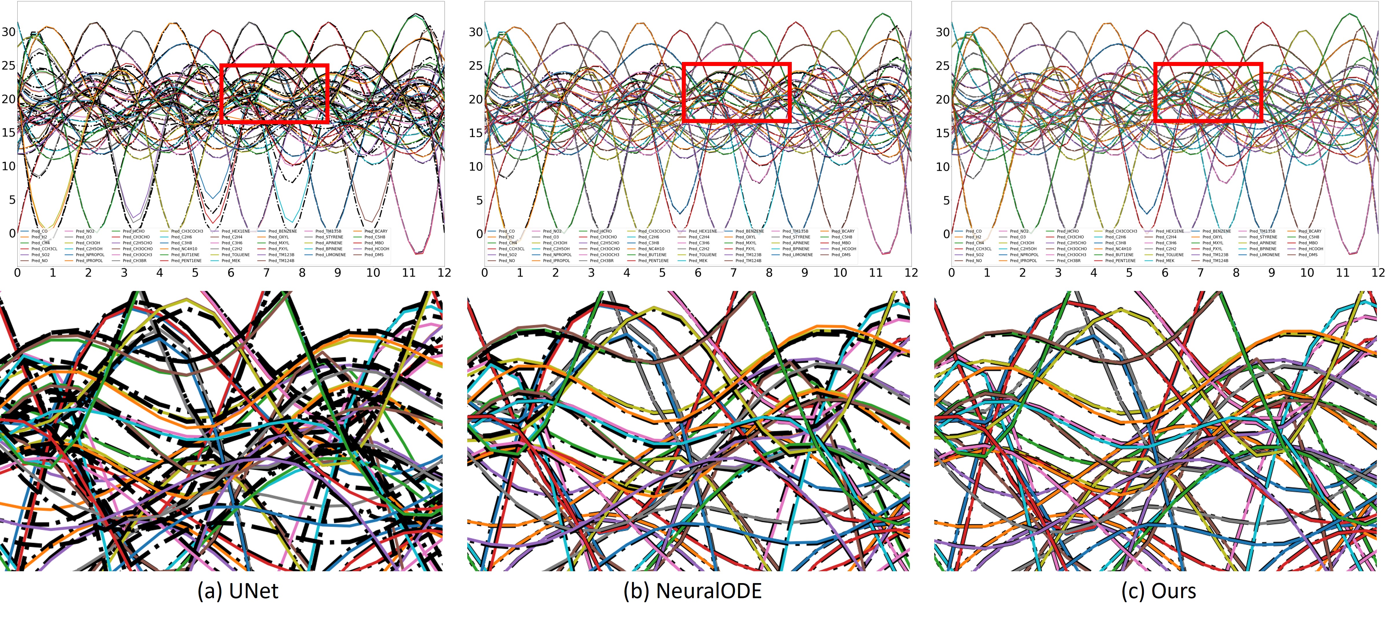
Figure 3: Visualization of the time evolution of chemistry in Task 1. In (a), (b), and (c), we show the ground truth as dashed black lines and the predictions as solid lines with different colors. We also enlarge the region in red boxes to highlight the prediction errors.

Task	Model	Validaton			Testing			Running time (s)	MACs (M)
		RMSE	MAE	MBE	RMSE	MAE	MBE
Task 1	UNet	0.4210	0.3292	0.2232	0.4267	0.3316	0.2152	5.15e-5	10.45
	NeuralODE	0.3959	0.2741	0.0003	0.3958	0.2738	0.0002	1.06e-4	10.95
	Ours	0.0194	0.0086	-1.9e-5	0.0652	0.0441	-0.0028	5.12e-5	13.77
Task 2	UNet	0.4283	0.2984	0.0163	0.4291	0.2988	0.0166	5.06e-5	14.11
	NeuralODE	0.2136	0.1244	0.0094	0.2144	0.1247	0.0074	1.26e-4	12.13
	Ours	0.1156	0.0312	-0.0037	0.1174	0.0316	-0.0037	5.55e-5	13.94
Task 3	UNet	0.3096	0.1933	-0.0009	0.3090	0.1932	-0.0009	9.74e-5	45.03
	NeuralODE	0.2102	0.1079	-0.0015	0.2086	0.1078	-0.0016	2.18e-4	42.03
	Ours	0.0748	0.0357	0.0003	0.0749	0.0359	0.0003	1.07e-4	44.34

Table 2: Compare state-of-the-art methods on three tasks for chemical concentration prediction. We test different methods on both validation and testing sets. For all metrics, the lower the values, the better prediction is achieved.

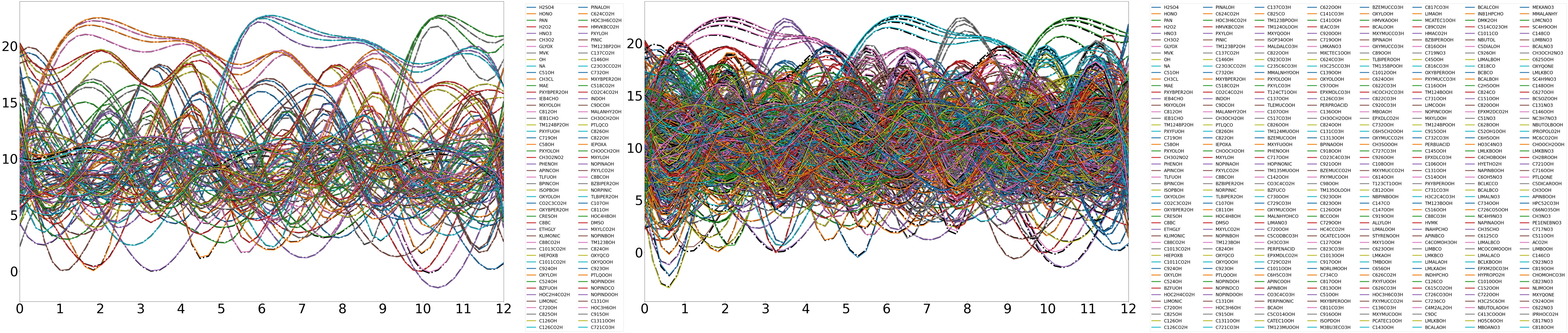
Figure 4: Visualization of the time evolution of chemistry in Task 2 and 3. In (a), and (b), we show the ground truth as dashed black lines and the predictions as solid lines with different colors. Task 2 predicts 100 unknown chemical components and Task 3 predicts 400 unknown chemical components.

4.2 Overall comparison with state of the arts

To demonstrate the efficiency of our proposed ChemNNE , we compare it with two state-of-the-art methods: UNet (Williams et al. (2024)), NeuralODE (Chen et al. (2018)), which are widely used in neural ODE/PDE processes. The comparison is shown in Table 2. We compare different approaches on both validation and testing datasets in logarithm scales. We also show the model complexity by running time (seconds) and number of Multiply–accumulate operations (MACs). Compared to NeuralODE and UNet, we can observe that using our proposed ChemNNE can achieve the best performance in terms of RMSE, MAE and MBE. For instance, ours can improve the RMSE by about 0.28 $\sim$ 0.41 in Task 1, 0.1$\sim$ 0.3 in Task 2, and 0.14$\sim$ 0.23 in Task 3. Comparing different tasks, we can see that the improvements from Task 1 to Task 3 are reduced which also indicates that the modeling difficulty is increased when more unknown chemical components are estimated. From the computation complexity, ours has a comparable number of operations as the other two and achieves a similar running speed. As the baseline, the numerical chemical model takes 0.05 seconds to run one simulation. It indicates that ours can be used as a fast emulator to accelerate the chemical modeling process. For visualization, we take different results on Task 1 and visualize them in Figure 3. We enlarge the red-box regions to demonstrate better the differences between ground truth (dashed black lines) and predictions (solid color lines). We can see that using ours can accurately align with the ground truth. For Task 2 and 3, we show the results in Figure 4. We can see that the color lines are overlapped with the dashed black lines, which indicates that our predictions align well with the ground truth values.

Components					Task 1			Task 2			Task 3
AE	Attn	Time emb	INR	FNO	RMSE	MAE	MBE	RMSE	MAE	MBE	RMSE	MAE	MBE
✓					0.3776	0.1876	0.0155	0.3976	0.2995	0.0368	0.5113	0.4010	0.0301
✓	✓				0.1252	0.0662	0.0044	0.2615	0.1589	0.0152	0.2455	0.1675	0.0089
✓		✓			0.3240	0.1665	0.0147	0.3589	0.2745	0.0235	0.5012	0.3370	0.0125
✓			✓		0.2256	0.1825	0.0035	0.1956	0.0899	0.0168	0.4888	0.3412	0.0115
✓				✓	0.0707	0.0486	0.0033	0.1389	0.0785	-0.0082	0.0789	0.0386	-0.0023
✓	✓	✓			0.0649	0.0441	-0.0029	0.1373	0.0675	0.0068	0.0768	0.0375	-0.0010
✓	✓	✓	✓		0.0201	0.0109	0.0041	0.1182	0.0324	0.0031	0.1201	0.0328	0.0032
✓	✓	✓	✓	✓	0.0194	0.0086	-1.9e-5	0.1156	0.0312	-0.0037	0.0748	0.0357	0.0003

Table 3: Comparison on different key components of our proposed ChemNNE . We report the results on validation datasets and for all metrics, lower values mean better performance.

Task		MSE (baseline)	MSE+Derivs	MSE+Derivs+Idn	MSE+Derivs+Mass	MSE+Derivs+Idn+Mass
Task 1	RMSE	0.0315	0.0268	0.0225	0.0210	0.0194
	MAE	0.0126	0.0102	0.0094	0.0089	0.0086
	MBE	0.0008	2.9e-5	3.4e-5	2.8e-5	-1.9e-5
Task 2	RMSE	0.1876	0.1820	0.1502	0.1501	0.1156
	MAE	0.0589	0.0566	0.0408	0.0386	0.0312
	MBE	0.0089	0.0091	-0.0076	0.0064	-0.0037
Task 3	RMSE	0.0896	0.0895	0.0820	0.0766	0.0748
	MAE	0.0523	0.0510	0.0461	0.0447	0.0357
	MBE	0.0015	0.0015	0.0008	0.0010	0.0003

Table 4: Comparison on different loss terms of our proposed ChemNNE . We report the results on the validation dataset and we can see that the combination of all losses achieves the best performance.

4.3 Ablation studies

We conduct several ablations to test the key components of the proposed ChemNNE and report the results in Table 3.

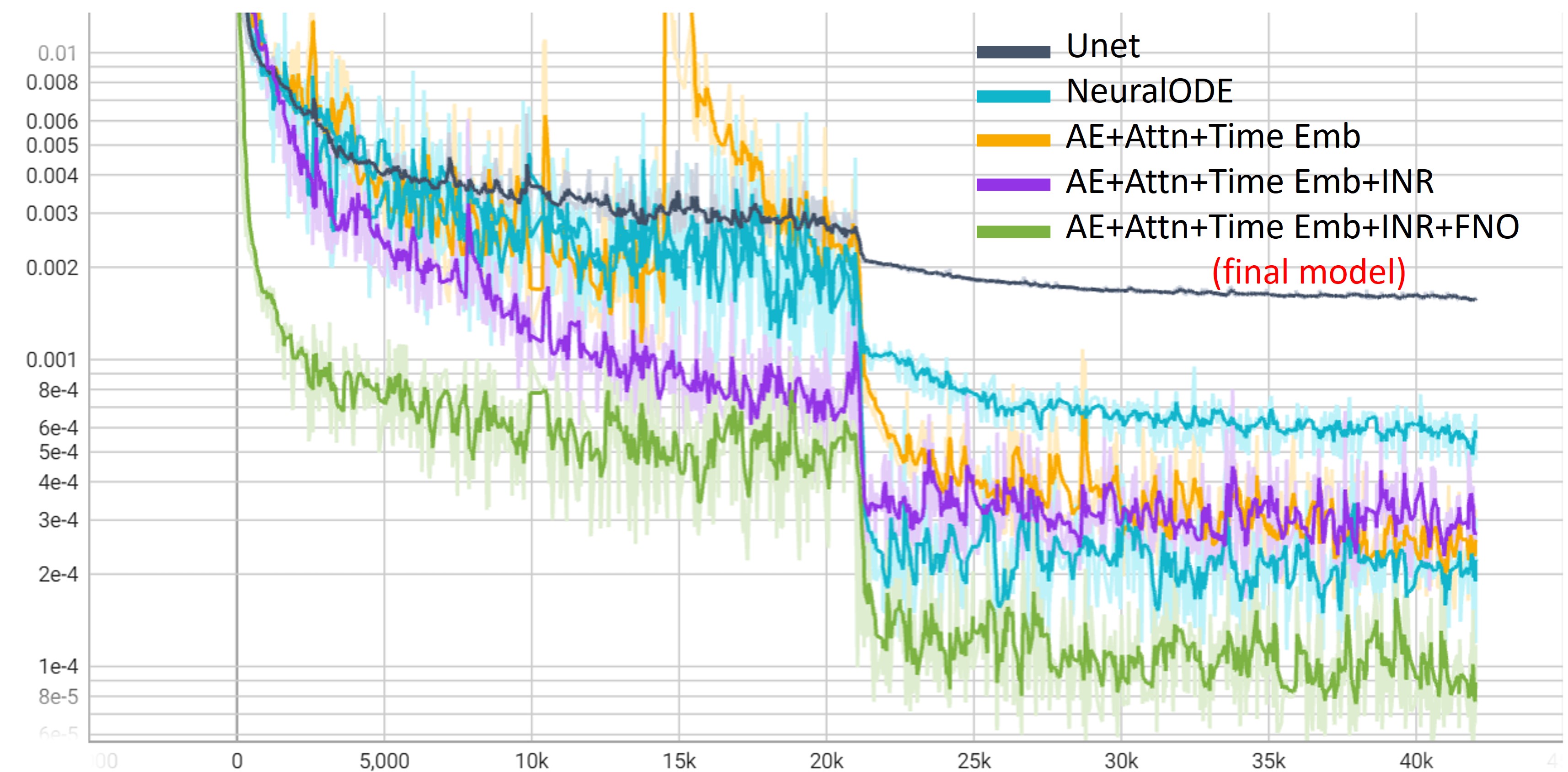
Figure 5: Training loss comparison among ours and others. We show different approaches in different colors, and we can see the improvements of using our proposed ChemNNE in both convergence speed and final loss.

We use the validation dataset of all three Tasks to demonstrate the effects of different key components, including AE (AutoEncoder), attention (attn), time embedding (Time emb), INR, FNO, and their combinations. Using AE is our baseline. We can see that the last row is our final model, which shows the best performances in all metrics. Individually, we can see that using attention and FNO can achieve the most improvements by approximately 0.1 $\sim$ 0.4 in terms of RMSE. Using time embedding and INR can also improve the RMSE by about 0.01 $\sim$ 0.2.

To further demonstrate the effect of the key components of attention and FNO, we visualize the training loss convergences in Figure 5. Compared to Unet and NeuralODE, we can see that ours with attention and/or FNO achieves the fastest convergence speed and lowest training loss.

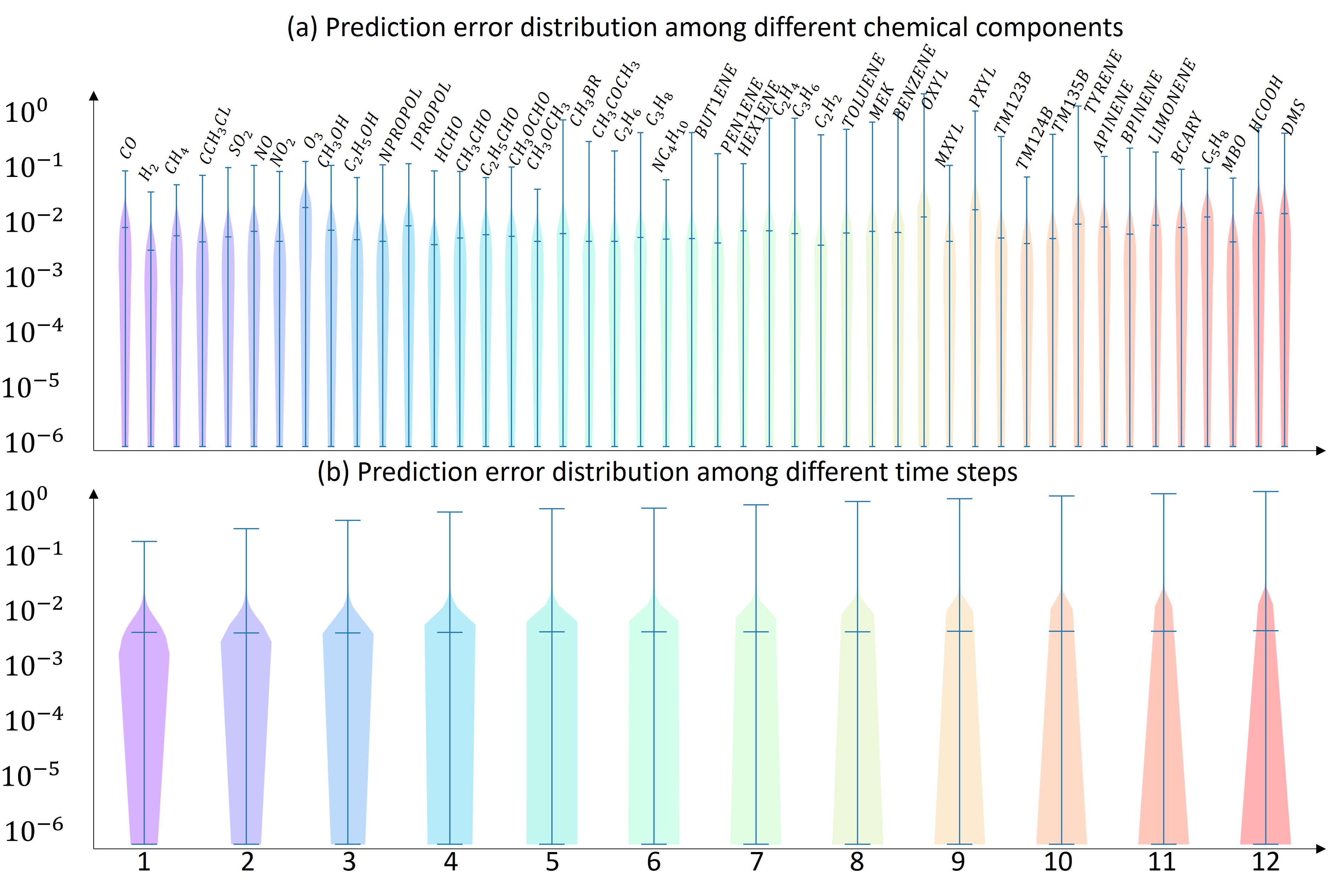
Figure 6: Validation error distribution visualization via violin plots. We show the error distributions (using the logarithm scale for better visualization) of different chemical components (a), and different time steps (b). The narrower the color shades, the smaller the error distributions.

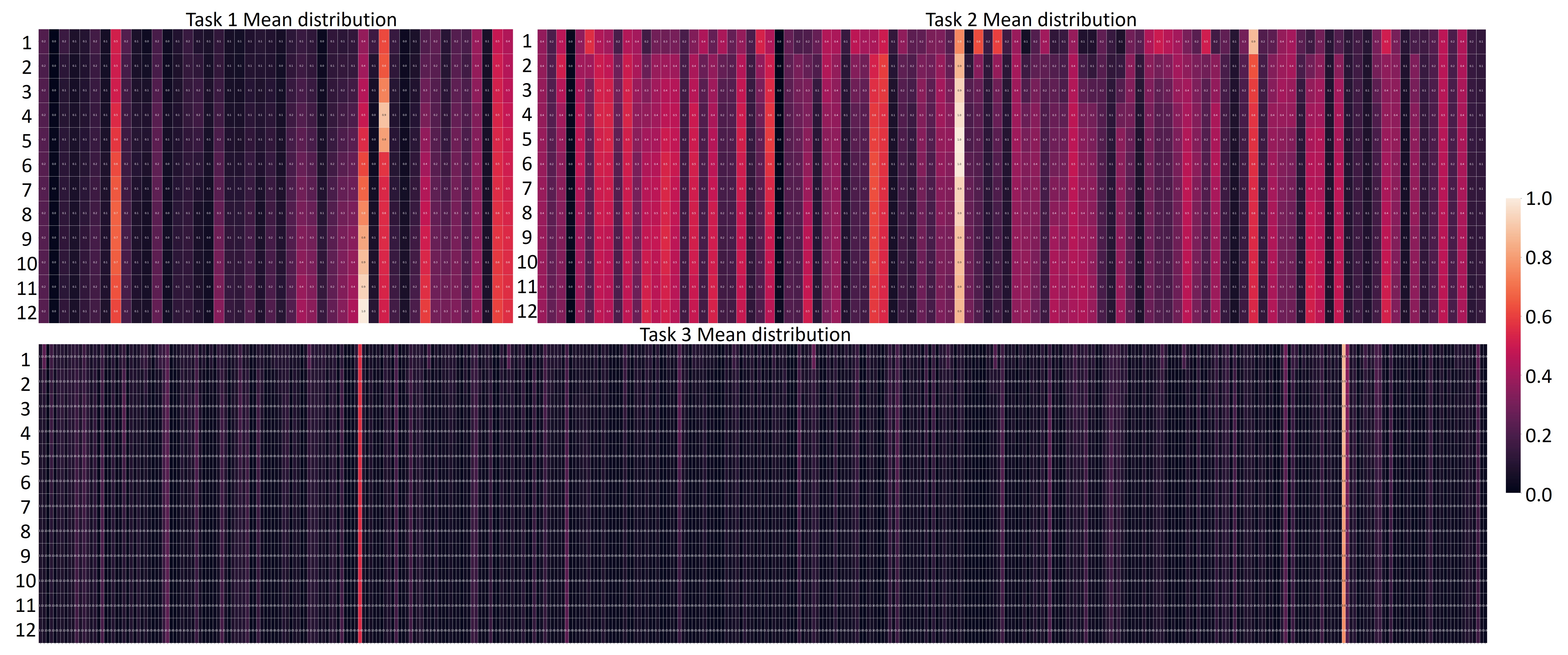
Figure 7: Mean distribution of validation errors of three tasks. We show the mean values of error distributions on three tasks, where the horizontal axis represents different chemical components and the vertical axis represents different time steps.

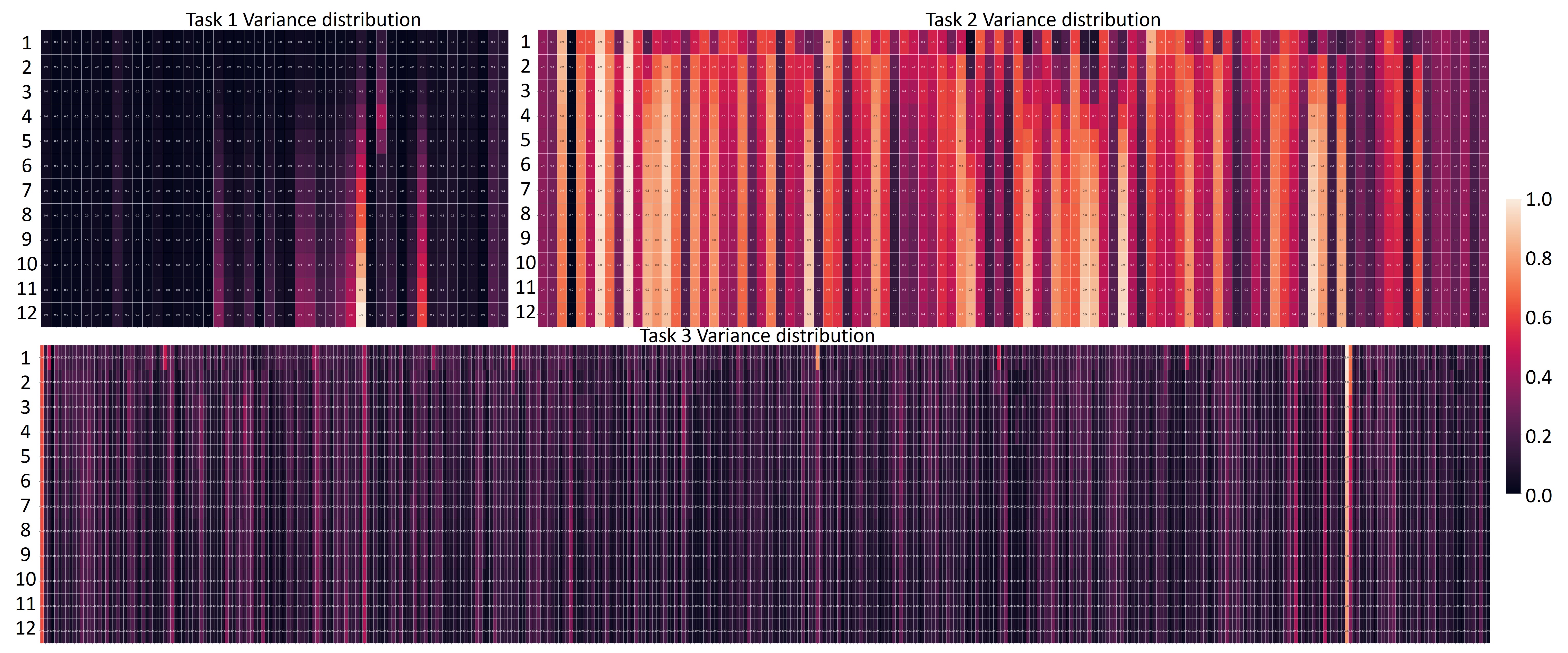
Figure 8: Variance distribution of validation errors of three tasks. We show the variance values of error distributions on three tasks, where the horizontal axis represents different chemical components and the vertical axis represents different time steps.

Finally, we train our proposed ChemNNE with different loss combinations, so that we can validate the effects of using physical-informed losses for model optimization. As the baseline, we train the model with MSE loss ($L_{recon}$), and then we individually add other losses to retrain the model, including first- and second-order derivative losses (Derivs), identity loss (IDN), and mass conservation loss (Mass). In Table 4, we show the RMSE, MAE, and MBE results on three tasks. Our observations are: 1) from columns 2 and 3, we can see that using identity and mass conservation losses have a more significant loss drop, about 0.03 $\sim$ 0.1 in RMSE, 2) using derivative loss has more visible effects on Task1 than Task 2 and 3 because Task 1 is intraperiod chemical prediction, that is, the derivative can better constrain the chemical reaction process for accurate estimation.

4.4 Statistical analysis

To study in depth the proposed ChemNNE on the ability of chemical modeling, we study the error distributions among different chemical components and time steps, so that we can see whether the model can estimate the patterns for each individual component, as well as long-term regression. In Figure 6, we show the error distribution in Task 1. We can see that 1) the model performs unevenly on different chemical components in terms of means and variances, and 2) the errors increase when predicting further steps in the future.

For Tasks 2 and 3, we have a much larger number of chemical components, 100 to 400 chemical components, for computation. To efficiently demonstrate the model performance, we show the 2D heatmap of mean and variance distributions on the validation datasets. Figure 7 and Figure 8 show the mean and variance of error distributions in all three tasks. The brighter the color, the higher the errors the model produces. From Figure 7, we can observe that the average performance differences depend on the specific chemical components. From Figure 8, we can see that the error variances vary because of the time steps. The farther the future step to predict, the higher the variances the model gets. The patterns also match our observations in Figure 6.

Specifically, we are interested in the chemistry that the model fails to predict well. In Task 1, the top five highest errors come from $O_{3},OXYL,PXYL$, $HCOOH,DMS$. Ozone ($O_{3}$) is one of the main oxidants in the atmosphere and reacts with many compounds. Therefore its predictions are related to the concentrations of many other compounds. 1,2-dimetylbenzene ($OXYL$) and 1,4-dimethylbenzene ($PXYL$) are aromatics which react mainly with the hydroxyl radical ($OH$). OH is formed inside the model and is the most important oxidant of the atmosphere during daytime and reactive towards nearly all compounds. The uncertainty for $OXYL$ and $PXYL$ is mainly related to the performance of OH and the same is the reason for dimethylsulphide ($DMS$) and formic acid ($HCOOH$). For Task 2, the top four highest errors come from $HOC_{2}H_{4}CO_{2}H,PXYLCO_{2}H,KLIMONIC,C_{88}CO_{2}H$. For Task 3, the top two highest errors come from $OXYQOOH,LMLKBCO$. All these compounds are higher-order reaction products of our initial compounds and are formed after several reactions with ozone, the nitrate and the hydroxyl radical. The most promising way to decrease the uncertainties of these compounds is to increase our training data set in the future.

5 Conclusion

In this paper, we propose the first work on a neural network emulator for fast chemical modeling, dubbed ChemNNE . We utilize the numerical simulation to generate a large-scale chemical dataset which is used to train the proposed ChemNNE , so that it can learn the hidden inter- and intra-correlations among chemical molecules. We propose to combine attention and neural ODE operations to model the time-dependent chemical reactions. Meanwhile, we lift the neural ODE as a Fourier domain convolution such that we can efficiently model the global continuous ODE. The time embedding and INR operators also help model the oscillation patterns to mimic the concentration changes of chemistry. To demonstrate the efficiency and effectiveness of the proposed model, we test it on three tasks, including intraperiod, interperiod and hybridperiod chemical predictions. Extensive experiments show that ours achieves the best performance in both accuracy and running speed. This work paves a new direction in AI for atmospheric chemistry, and we will continue to explore graph neural networks, equivalent neural networks, and other advanced models to integrate chemical knowledge for physics-informed processing.

References

- Abramson et al. (2024) Abramson, J., Adler, J., Dunger, J., et al., 2024. Accurate structure prediction of biomolecular interactions with alphafold 3. Nature , 493–500.
- Bassetti et al. (2023) Bassetti, S., Hutchinson, B., Tebaldi, C., Kravitz, B., 2023. Diffesm: Conditional emulation of earth system models with diffusion models. International Conference on Learning Representation .
- Bhatnagar et al. (2019) Bhatnagar, S., Afshar, Y., Pan, S., Duraisamy, K., Kaushik, S., 2019. Prediction of aerodynamic flow fields using convolutional neural networks 64, 525–545.
- Bi et al. (2023) Bi, K., Xie, L., Zhang, H., et al., 2023. Accurate medium-range global weather forecasting with 3d neural networks. Nature 619, 533–538.
- Biloš et al. (2021) Biloš, M., Sommer, J., Rangapuram, S.S., Januschowski, T., Günnemann, S., 2021. Neural flows: Efficient alternative to neural odes. Advances in neural information processing systems 34, 21325–21337.
- Bodnar et al. (2024) Bodnar, C., Bruinsma, W.P., et al., 2024. Aurora: A foundation model of the atmosphere. arXiv 2405.13063.
- Boiko et al. (2023) Boiko, D., MacKnight, R., Kline, B., et al., 2023. Autonomous chemical research with large language models. Nature 624, 570–578.
- Bonev et al. (2023) Bonev, B., Kurth, T., Hundt, C., et al., 2023. Spherical fourier neural operators: learning stable dynamics on the sphere, in: Proceedings of the 40th International Conference on Machine Learning.
- Castruccio et al. (2014) Castruccio, S., McInerney, D.J., Stein, M.L., Liu, F., et al., 2014. Statistical emulation of climate model projections based on precomputed gcm runs. Journal of Climate 27, 1829–1844.
- Chen et al. (2018) Chen, R.T.Q., Rubanova, Y., Bettencourt, J., Duvenaud, D., 2018. Neural ordinary differential equations , 6572––6583.
- Chithrananda et al. (2020) Chithrananda, S., Grand, G., Ramsundar, B., 2020. Chemberta: Large-scale self-supervised pretraining for molecular property prediction. ArXiv abs/2010.09885. URL: https://api.semanticscholar.org/CorpusID:224803102.
- Clusius et al. (2022) Clusius, P., Xavier, C., Pichelstorfer, L., Zhou, P., Olenius, T., Roldin, P., Boy, M., 2022. Atmospherically relevant chemistry and aerosol box model – arca box (version 1.2). Geoscientific Model Development 15, 7257–7286.
- Geneva and Zabaras (2020) Geneva, N., Zabaras, N., 2020. Modeling the dynamics of pde systems with physics-constrained deep auto-regressive networks 403.
- Goodall and Lee (2020) Goodall, R.E.A., Lee, A.A., 2020. Predicting materials properties without crystal structure: deep representation learning from stoichiometry. Nature Communication 6280.
- Goswami et al. (2024) Goswami, S., Jagtap, A.D., Babaee, H., Susi, B.T., Karniadakis, G.E., 2024. Learning stiff chemical kinetics using extended deep neural operators, in: CHAME.
- Hayat et al. (2020) Hayat, M.A., Stein, G., Harrington, P., Lukic, Z., Mustafa, M., 2020. self supervised representation learning for astronomical images. The Astrophysical Journal Letters .
- Hochreiter and Schmidhuber. (1997) Hochreiter, S., Schmidhuber., J., 1997. Long short-term memory. Neural Comput. .
- Jenkin et al. (2015) Jenkin, M., Young, J., Rickard, A., 2015. The mcm v3.3.1 degradation scheme for isoprene. Atmospheric Chemistry and Physics 15.
- Jenkin et al. (1997) Jenkin, M.E., Saunders, S.M., Pilling, M.J., 1997. The tropospheric degradation of volatile organic compounds: a protocol for mechanism development. Atmospheric Environment 31, 81–104.
- Jiang et al. (2020) Jiang, C., Esmaeilzadeh, S., Azizzadenesheli, K., et al., 2020. Meshfreeflownet: a physics-constrained deep continuous space-time super-resolution framework, in: Proceedings of the International Conference for High Performance Computing, Networking, Storage and Analysis.
- K. et al. (2024) K., N., Li, Z., Liu, B., et al., 2024. Neural operator: learning maps between function spaces with applications to pdes. J. Mach. Learn. Res. 24.
- Khoo et al. (2020) Khoo, Y., Lu, J., Ying, L., 2020. Solving parametric pde problems with artificial neural networks 32, 421–435.
- Lam and et al. (2023) Lam, R., et al., 2023. Learning skillful medium-range global weather forecasting. Science 382, 1416–1421.
- Li et al. (2019) Li, S., Jin, X., Xuan, Y., Zhou, X., Chen, W., Wang, Y.X., Yan, X., 2019. Enhancing the locality and breaking the memory bottleneck of transformer on time series forecasting. Advances in neural information processing systems 32.
- Li et al. (2020) Li, Z., Kovachki, N., Azizzadenesheli, K., Liu, B., Bhattacharya, K., Stuart, A., Anandkumar, A., 2020. Fourier neural operator for parametric partial differential equations.
- Li et al. (2023) Li, Z., Kovachki, N.B., Choy, C., Li, B., Kossaifi, J., Otta, S.P., Nabian, M.A., Stadler, M., Hundt, C., Azizzadenesheli, K., Anandkumar, A., 2023. Geometry-informed neural operator for large-scale 3d PDEs, in: Thirty-seventh Conference on Neural Information Processing Systems.
- Lu et al. (2021) Lu, L., Jin, P., Pang, G., et al., 2021. Learning nonlinear operators via deeponet based on the universal approximation theorem of operators, in: Nat Mach Intell, pp. 218–229.
- Massaroli et al. (2020) Massaroli, S., Poli, M., Park, J., Yamashita, A., Asama, H., 2020. Dissecting neural odes. Advances in Neural Information Processing Systems 33, 3952–3963.
- Mildenhall et al. (2020) Mildenhall, B., Srinivasan, P.P., Tancik, M., Barron, J.T., Ramamoorthi, R., Ng, R., 2020. Nerf: Representing scenes as neural radiance fields for view synthesis, in: ECCV.
- Norcliffe et al. (2020) Norcliffe, A., Bodnar, C., Day, B., Simidjievski, N., Liò, P., 2020. On second order behaviour in augmented neural odes. Advances in neural information processing systems 33, 5911–5921.
- OpenAI and et al. (2023) OpenAI, et al., 2023. Gpt-4 technical report. International Conference on Learning Representation .
- Pokkunuru et al. (2023) Pokkunuru, A., Rooshenas, P., Strauss, T., Abhishek, A., Khan, T., 2023. Improved training of physics-informed neural networks using energy-based priors: A study on electrical impedance tomography, in: International Conference on Learning Representation.
- Portillo et al. (2020) Portillo, S.K., Parejko, J.K., Vergara, J.R., Connolly, A.J., 2020. Dimensionality reduction of sdss spectra with variational autoencoders. The Astrophysical Journal 45.
- Radford et al. (2023) Radford, A., Kim, J., Xu, T., et al., 2023. Robust speech recognition via large-scale weak supervision, in: Proceedings of the 40th International Conference on Machine Learning.
- Raissi et al. (2019) Raissi, M., Perdikaris, P., Karniadakis, G.E., 2019. Physics-informed neural networks: A deep learning framework for solving forward and inverse problems involving nonlinear partial differential equations 378, 686––707.
- Raissi et al. (2020) Raissi, M., Yazdani, A., Karniadakis, G.E., 2020. Hidden fluid mechanics: Learning velocity and pressure fields from flow visualizations 367, 1026––1030.
- Ramesh et al. (2021) Ramesh, A., Pavlov, M., Goh, G., Gray, S., Voss, C., Radford, A., Chen, M., Sutskever, I., 2021. Zero-shot text-to-image generation, in: Meila, M., Zhang, T. (Eds.), Proceedings of the 38th International Conference on Machine Learning, pp. 8821–8831.
- Ren et al. (2023) Ren, P., Rao, C., Liu, Y., Ma, Z., Wang, Q., Wang, J.X., Sun, H., 2023. Physr: Physics-informed deep super-resolution for spatiotemporal data. Journal of Computational Physics , 112438.
- Roldin et al. (2019) Roldin, P., Ehn, M., Kurtén, T., et al., 2019. The role of highly oxygenated organic molecules in the boreal aerosol-cloud-climate system. Nat Commun 4370.
- Sandu et al. (2023) Sandu, A., Sander, R., et al., 2023. An adaptive auto-reduction solver for speeding up integration of chemical kinetics in atmospheric chemistry models: implementation and evaluation within the kinetic pre-processor (kpp) version 3.0.0. JAMES 15.
- Sauer et al. (2023) Sauer, A., Lorenz, D., Blattmann, A., Rombach, R., 2023. Adversarial diffusion distillation. arXiv:2311.17042.
- Saunders et al. (2003) Saunders, S.M., Jenkin, M.E., Derwent, R.G., Pilling, M.J., 2003. Protocol for the development of the master chemical mechanism, mcm v3 (part a): tropospheric degradation of non-aromatic volatile organic compounds. Atmospheric Chemistry and Physics 3, 161–180.
- Sitzmann et al. (2020) Sitzmann, V., Martel, J.N., Bergman, A.W., Lindell, D.B., Wetzstein, G., 2020. Implicit neural representations with periodic activation functions, in: Proc. NeurIPS.
- Solaiman et al. (2019) Solaiman, I., Brundage, M., Clark, J., Askell, A., Herbert-Voss, A., Wu, J., Radford, A., Wang, J., 2019. Release strategies and the social impacts of language models. arXiv preprint arXiv:1908.09203 .
- Su et al. (2024) Su, J., Ma, J., Tong, S., Xu, E., Chen, M., 2024. Multiscale attention wavelet neural operator for capturing steep trajectories in biochemical systems, in: AAAI Conference on Artificial Intelligence, pp. 15100–15107.
- Touvron et al. (2023a) Touvron, H., Lavril, T., Izacard, G., Martinet, X., Lachaux, M.A., Lacroix, T., Rozière, B., Goyal, N., Hambro, E., Azhar, F., Rodriguez, A., Joulin, A., Grave, E., Lample, G., 2023a. Llama: Open and efficient foundation language models. arXiv preprint arXiv:2302.13971 .
- Touvron et al. (2023b) Touvron, H., Martin, L., Stone, K., Albert, P., et al, 2023b. Llama 2: Open foundation and fine-tuned chat models. arXiv preprint arXiv:2307.09288 .
- Vaswani et al. (2017) Vaswani, A., Shazeer, N., Parmar, N., Uszkoreit, J., Jones, L., Gomez, A., Polosukhin, I., 2017. Attention is all you need. Advances in neural information processing systems , 5998–6008.
- Volk et al. (2023) Volk, A.A., Epps, R.W., Yonemoto, D.T., Masters, B.S., et al., 2023. Alphaflow: autonomous discovery and optimization of multi-step chemistry using a self-driven fluidic lab guided by reinforcement learning. Nature Communication .
- Williams et al. (2024) Williams, C., Falck, F., Deligiannidis, G., Holmes, C., Doucet, A., Syed, S., 2024. A unified framework for u-net design and analysis, in: Proceedings of the 37th International Conference on Neural Information Processing Systems.
- Wu et al. (2021) Wu, H., Xu, J., Wang, J., Long, M., 2021. Autoformer: Decomposition transformers with auto-correlation for long-term series forecasting. Advances in neural information processing systems .
- Wu et al. (2023) Wu, Z., Wang, J., Du, H., et al., 2023. Chemistry-intuitive explanation of graph neural networks for molecular property prediction with substructure masking. Nat Commun 14.
- Xu et al. (2023) Xu, Z., Sangineto, E., Sebe, N., 2023. Stylerdalle: Language-guided style transfer using a vector-quantized tokenizer of a large-scale generative model, in: Proceedings of the IEEE/CVF International Conference on Computer Vision (ICCV), pp. 7601–7611.
- Yildiz et al. (2019) Yildiz, C., Heinonen, M., Lahdesmaki, H., 2019. Ode2vae: Deep generative second order odes with bayesian neural networks. Advances in Neural Information Processing Systems 32.
- Zhou et al. (2021) Zhou, H., Zhang, S., Peng, J., Zhang, S., Li, J., Xiong, H., Zhang, W., 2021. Informer: Beyond efficient transformer for long sequence time-series forecasting. AAAI Conference on Artificial Intelligence .
- Zhou et al. (2022) Zhou, T., Ma, Z., Wen, Q., Wang, X., Sun, L., Jin, R., 2022. Fedformer: Frequency enhanced decomposed transformer for long-term series forecasting .
- Zhu et al. (2019) Zhu, Y., Zabaras, N., Koutsourelakis, P.S., Perdikaris, P., 2019. Physics-constrained deep learning for high-dimensional surrogate modeling and uncertainty quantification without labeled data 394, 56–81.