Exclusive photoproduction of $\eta_{c}\gamma$ pairs with large invariant mass

Abstract

In this preprint we analyzed the exclusive photoproduction of $\eta_{c}\gamma$ pairs in the collinear factorization framework and evaluated its cross-section in leading order in the strong coupling $\alpha_{s}$. We found that this process is mostly sensitive to the behavior of the unpolarized gluon GPD $H_{g}$ in the Efremov-Radyushkin-Brodsky-Lepage kinematics. We estimated numerically the cross-section and the expected counting rates in the kinematics of middle-energy photoproduction experiments which can be realized at the future Electron-Ion Collider and in the kinematics of ultraperipheral collisions at LHC. We found that the cross-section is sufficiently large for dedicated experimental study.

I Introduction

The Generalized Parton Distributions (GPDs) encode information about the nonperturbative dynamics of different parton flavors in the hadronic target, and for this reason have been intensively studied both theoretically and experimentally in the last two decades Diehl:2000xz ; Goeke:2001tz ; Diehl:2003ny ; Guidal:2013rya ; Boer:2011fh ; Dutrieux:2021nlz ; Burkert:2022hjz ; AbdulKhalek:2021gbh ; Accardi:2012qut . At present, it is not possible to evaluate the GPDs from the first principles, and for this reason studies of these objects rely on phenomenological extractions from experimental data. Most of the currently available phenomenological parametrizations of the GPDs are based on experimental studies of $2\to 2$ processes, like Deeply Virtual Compton Scattering (DVCS) and Deeply Virtual Meson Production (DVMP). However, as was discussed in  Kumericki:2016ehc ; Bertone:2021yyz ; Moffat:2023svr , these channels do not fix uniquely the GPDs due to poor sensitivity of the physical observables to behavior of the GPDs in some kinematic regions (the so-called “shadow GPD problem”). While the experimental data allow to constrain reasonably well some of the GPDs, at present these constraints are very loose in the Efremov-Radyushkin-Brodsky-Lepage (ERBL) kinematics, for the transversity GPDs, and the GPDs of gluons in general Guo:2023ahv . For this reason, the interest of the community has shifted towards search of new channels which could be used for complementary studies, and various $2\to 3$ processes have been suggested as novel tools for studies of the GPDs GPD2x3:9 ; GPD2x3:8 ; GPD2x3:7 ; GPD2x3:6 ; GPD2x3:5 ; GPD2x3:4 ; GPD2x3:3 ; GPD2x3:2 ; GPD2x3:1 ; Duplancic:2022wqn ; Qiu:2024mny ; Qiu:2023mrm ; Deja:2023ahc ; Siddikov:2022bku ; Siddikov:2023qbd . Due to sensitivity of each process to unique combination of different GPD flavors in different kinematic domains, all these channels naturally complement each other, and the quest for new channels remains open. As was discussed in  GPD2x3:10 ; GPD2x3:11 , the factorization theorems for such processes in general require presence of hard scale and good kinematic separation of the produced hadrons. Most of the above-mentioned studies focused on production of light meson or photon pairs, whose amplitudes are dominated by quark GPDs (both in chiral odd and chiral even sectors). The gluon GPDs also may contribute in some of these channels, however usually these contributions are commingled with contribution of quarks, complicating the phenomenological analysis. Furthermore, recently it was discovered in Duplancic:2024opc ; Nabeebaccus:2023 that the gluonic coefficient function of the processes like $\gamma p\to\pi^{0}\gamma p$ suffers from nontrivial overlapping singularities, and the applicability of the collinear factorization is justified only if the distribution amplitude of produced light meson vanishes rapidly enough at the endpoints.

In order to take advantage of the $2\to 3$ processes for analysis of the gluon GPDs, we suggest to study the production of heavy quarkonia-photon pairs. Due to heavy mass of the quarkonia, which plays the role of natural hard scale, it is possible to use the perturbative methods even in the photoproduction regime Korner:1991kf ; Neubert:1993mb , and avoid many soft and collinear singularities which may occur in diagrams with massless quarks. The hadronization of $\bar{Q}Q$ pair into final state quarkonium is described in NRQCD framework, which allows to incorporate systematically various perturbative corrections Bodwin:1994jh ; Maltoni:1997pt ; Brambilla:2008zg ; Feng:2015cba ; Brambilla:2010cs ; Cho:1995ce ; Cho:1995vh ; Baranov:2002cf ; Baranov:2007dw ; Baranov:2011ib ; Baranov:2016clx ; Baranov:2015laa . The single-quarkonium production $\gamma p\to J/\psi\,p$ has been studied in detail both theoretically and experimentally DVMPcc1 ; DVMPcc2 ; DVMPcc3 ; DVMPcc4 , however it shares all the above-mentioned limitations of DVCS and DVMP. The process $\gamma p\to J/\psi\,\gamma p$ requires $C$-odd exchanges in the $t$-channel, and for this reason is strongly suppressed. However, the process $\gamma p\to\eta_{c}\,\gamma p$ presents an interesting opportunity for study of the gluon GPDs. Previously this channel has been studied in HarlandLang:2018ytk , assuming that it proceeds via a radiative decay of higher excited states (mainly $\gamma p\to J/\psi p\to\eta_{c}\gamma\,p$). Though this mechanism has a relatively large cross-section, it is controlled by the $J/\psi$ photoproduction cross-section and thus does not bring any new information for studies of GPDs. Fortunately, it is possible to eliminate this contribution imposing cuts on invariant mass of $\eta_{c}\gamma$ pair. In this paper, we will focus on production of $\eta_{c}\gamma$ pairs with large invariant mass, $M_{\gamma\eta_{c}}\geq 3.5-4\,{\rm GeV}^{2}$, where the feed-down contributions are negligible. This kinematic regime may be studied in low- and middle-energy photon-proton collisions in ultraperipheral kinematics at LHC, as well as electron-proton collisions at the future Electron Ion Collider (EIC) Accardi:2012qut ; AbdulKhalek:2021gbh ; Burkert:2022hjz and possible experiments at JLAB after 22 GeV upgrade Accardi:2023chb .

The suggested $\eta_{c}\gamma$ pair photoproduction (with undetected photon) is also interesting as a potential background to the $\eta_{c}$ photoproduction $\gamma p\to\eta_{c}p.$ The latter subprocess conventionally has been considered as one of the most promising channels for studies of odderons Odd4 ; Odd5 ; Odd6 ; Odd7 , and significant efforts have been dedicated to its theoretical understanding and experimental detection. The $\eta_{c}\gamma$ pair photoproduction does not require $C$-odd exchanges in $t$-channel, and for this reason could constitute a sizable background which sets the limits on detectability of odderons via $\eta_{c}$ photoproduction at future experiments.

The paper is structured as follows. Below in Section II we discuss in detail the kinematics of the process and the framework for evaluation of the amplitude of the process. In Section III we present our numerical estimates for cross-sections and counting rates of the process. In subsection III.3 we compare the photoproduction cross-sections for $\eta_{c}$ and $\eta_{c}\gamma$ with integrated out photon. Finally, in Section IV we draw conclusions.

II Theoretical framework

For analysis of the $\eta_{c}\gamma$ -photoproduction we may use the framework developed in GPD2x3:8 ; GPD2x3:9 for exclusive photoproduction of light meson-photon pairs $\gamma\pi,\,\gamma\rho$ with large invariant mass. The extension of those results to $\eta_{c}\gamma$ photoproduction is straightforward, however we can no longer disregard the mass of the meson $M_{\eta_{c}}$. It is more appropriate to consider $M_{\eta_{c}}$ as a hard scale on par with the invariant mass $M_{\gamma\eta_{c}}$, keeping it both in the kinematic relations and in coefficient functions. Both in electroproduction and ultraperipheral hadroproduction the spectrum of equivalent photons is dominated by quasi-real photons, so we’ll focus on the photoproduction by transversely polarized photons with zero virtuality $Q=0$. In the following subsections II.1,  II.2 we briefly introduce the main kinematic variables used for description of the process and discuss the evaluation of the amplitudes in the collinear factorization approach.

II.1 Kinematics of the process

In what follows, we will perform evaluations in the photon-proton collision frame, where the photon and the incoming proton move in the direction of axis $z$. We will use notations $q$ for the momentum of the incoming photon, $P_{{\rm in}},P_{{\rm out}}$ for the momentum of the proton before and after interaction, $k$ for the momentum of the emitted (outgoing) photon, and $p_{\eta_{c}}$ for the momentum of produced $\eta_{c}$ meson. In this frame the light-cone decomposition of the particles’ momenta may be written as GPD2x3:8 ; GPD2x3:9

$$q^{\mu} =n^{\mu}$$ (1)

$$P_{{\rm in}}^{\mu} =\left(1+\xi\right)p^{\mu}+\frac{m_{N}^{2}}{s(1+\xi)}n^{\mu},$$ (2)

$$P_{{\rm out}}^{\mu} =\left(1-\xi\right)p^{\mu}+\frac{m_{N}^{2}+\Delta_{\perp}^{2}}{s(1+\xi)}n^{\mu}+\Delta_{\perp}^{\mu},$$ (3)

$$p_{\eta_{c}}^{\mu} =\alpha_{\eta_{c}}n^{\mu}+\frac{\left(\boldsymbol{p}_{\perp}+\boldsymbol{\Delta}_{\perp}/2\right)^{2}+M_{\eta_{c}}^{2}}{\alpha_{\eta_{c}}s}p^{\mu}-\boldsymbol{p}_{\perp}-\frac{\boldsymbol{\Delta}_{\perp}}{2},$$ (4)

$$k^{\mu} =\left(1-\alpha_{\eta_{c}}\right)n^{\mu}+\frac{\left(\boldsymbol{p}_{\perp}-\boldsymbol{\Delta}_{\perp}/2\right)^{2}}{\left(1-\alpha_{\eta_{c}}\right)s}p^{\mu}+\boldsymbol{p}_{\perp}-\frac{\boldsymbol{\Delta}_{\perp}}{2},$$ (5)

where the basis light-cone vectors $p^{\mu},\,n^{\mu}$ are defined as

$$p^{\mu}=\frac{\sqrt{s}}{2}\left(1,0,0,1\right),\qquad n^{\mu}=\frac{\sqrt{s}}{2}\left(1,0,0,-1\right),\qquad p\cdot n=\frac{s}{2}.$$ (6)

In what follows we will use the invariant Mandelstam variables

$$S_{\gamma N} \equiv W^{2}=\left(q+P_{{\rm in}}\right)^{2}=s\left(1+\xi\right)+m_{N}^{2},$$ (7)

$$t =\left(P_{{\rm out}}-P_{{\rm in}}\right)^{2}=-\frac{1+\xi}{1-\xi}\Delta_{\perp}^{2}-\frac{4\xi^{2}m_{N}^{2}}{1-\xi^{2}}.$$ (8)

From Eq. (8) we can see that at given $\xi$, the invariant momentum transfer $t$ is bound by

$$t\leq t_{{\rm min}}=-\frac{4\xi^{2}m_{N}^{2}}{1-\xi^{2}}.$$

In what follows we will also use the variables

$$u^{\prime}=\left(p_{\eta_{c}}-q\right)^{2},\qquad t^{\prime}=\left(k-q\right)^{2},\qquad M_{\gamma\eta_{c}}^{2}=\left(k+p_{\eta_{c}}\right)^{2}$$ (9)

which are related as

$$-u^{\prime}-t^{\prime}=M_{\gamma\eta_{c}}^{2}-M_{\eta_{c}}^{2}-t.$$ (10)

The polarization vector of the incoming/outgoing real photon with momentum $\boldsymbol{k}$ and helicity $\lambda$ in the light-cone gauge is given by

$$\varepsilon_{T}^{(\lambda=\pm 1)}(\boldsymbol{k})=\left(0,\,\frac{\boldsymbol{e}_{\lambda}^{\perp}\cdot\boldsymbol{k}_{\perp}}{k^{+}},\boldsymbol{e}_{\lambda}^{\perp}\right),\qquad\boldsymbol{e}_{\lambda}^{\perp}=\frac{1}{\sqrt{2}}\left(\begin{array}[]{c}1\\ i\lambda\end{array}\right).$$ (11)

The parametrization  (1-5) implicitly implements various kinematic constraints on momenta of the produced particles which follow from onshellness of final state particles and energy-momentum conservation. In order to understand better these constraints, in the Figure (1) we have shown the kinematically allowed domains using conventional rapidities and transverse momenta of the final-state particles. The plot clearly shows that for a given energy $W$ and rapidities $y_{\eta_{c}},y_{\gamma}$, the transverse momenta $\boldsymbol{p}_{\eta_{c}}^{\perp}=-\boldsymbol{p}_{\perp}-\boldsymbol{\Delta}_{\perp}/2$ and $\boldsymbol{p}_{\gamma}^{\perp}=\boldsymbol{p}_{\perp}-\boldsymbol{\Delta}_{\perp}/2$ may take values only in a limited range. The color of each pixel in the Figure  (1) illustrates the value of the azimuthal angle $\phi$ between the transverse momenta of $\eta_{c},\gamma$ and the invariant mass $M_{\gamma\eta_{c}}$. In the Figure 2 we also have shown the relation of the variables $\xi,\,\alpha_{\eta_{c}}$ to rapidities $y_{\eta_{c}},y_{\gamma}$.

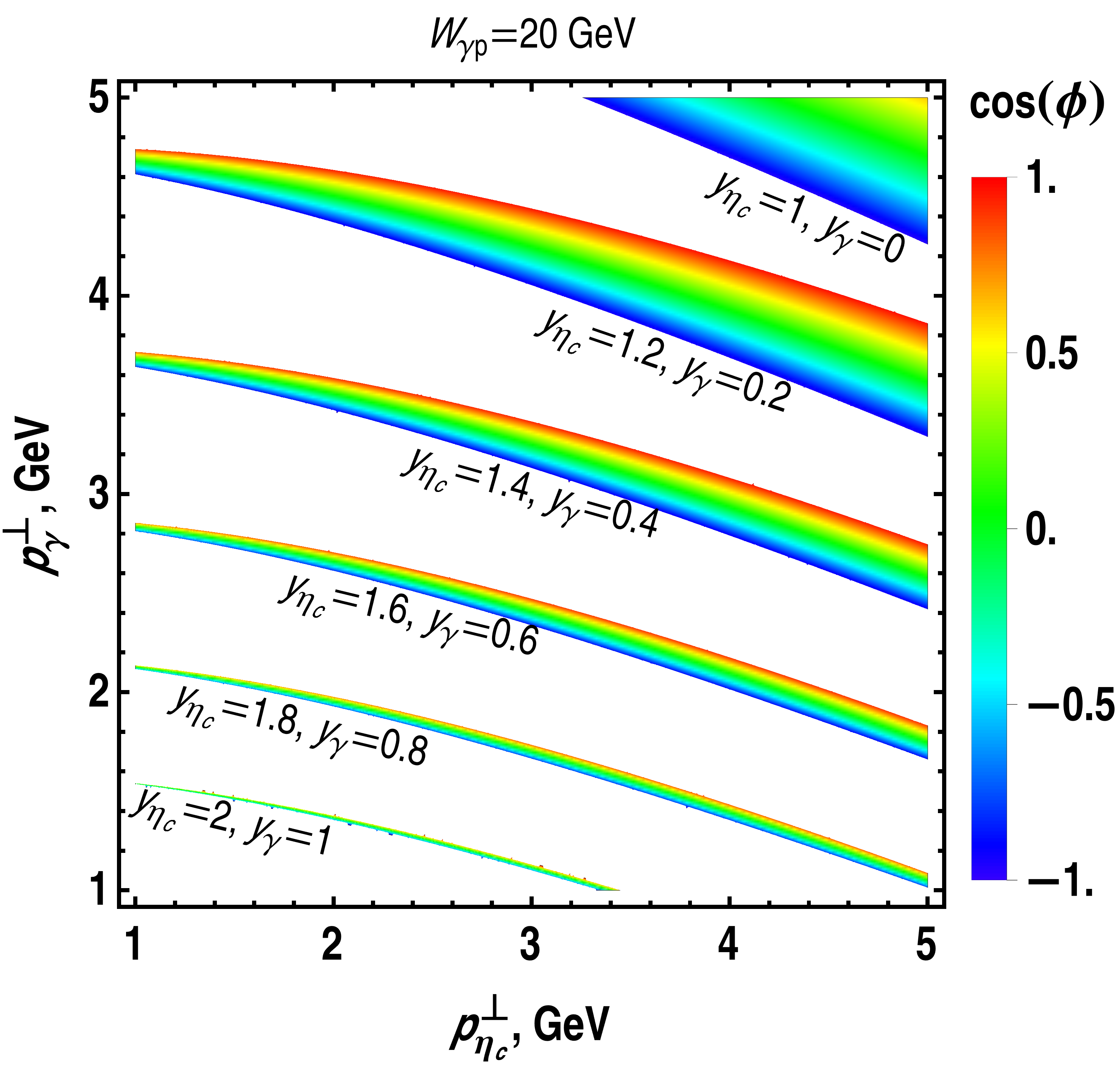
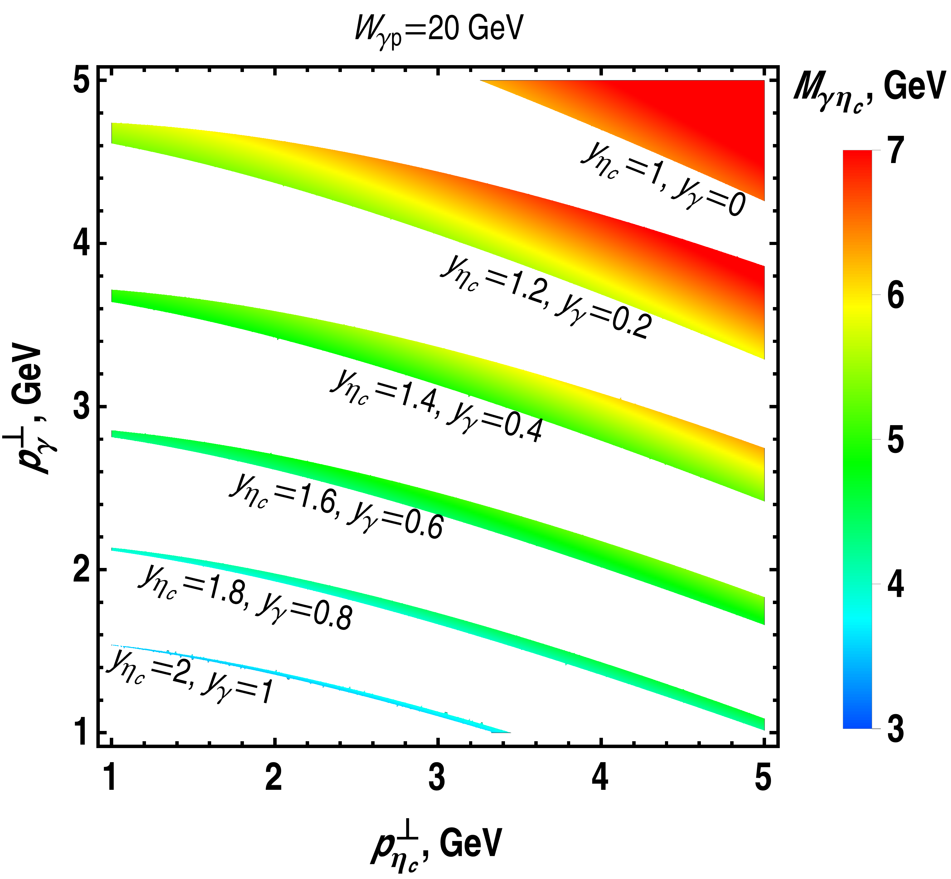
Figure 1: (Color online) Colored bands represent kinematically allowed region for $\eta_{c}\gamma$ pair production at fixed invariant energy $W$ and fixed rapidities $y_{\eta_{c}},\,y_{\gamma}$. For both particles we chose positive sign of rapidity in direction of the photon. Since photon moves in “minus” direction in (1), this corresponds to nonstandard definition of rapidity $y_{a}=\frac{1}{2}\ln\left(k_{a}^{-}/k_{a}^{+}\right),\qquad a=\eta_{c},\gamma$. The increase of rapidities implies increase of the longitudinal momenta, and thus in view of energy conservation corresponds to smaller transverse momenta. In the left plot the color of each pixel reflects the azimuthal angle $\phi$ between the transverse momenta $\boldsymbol{p}_{\eta_{c}}^{\perp}=-\boldsymbol{p}_{\perp}-\boldsymbol{\Delta}_{\perp}/2$ and $\boldsymbol{p}_{\gamma}^{\perp}=\boldsymbol{p}_{\perp}-\boldsymbol{\Delta}_{\perp}/2$. Similarly, in the right plot the color reflects the value of invariant mass $M_{\gamma\eta_{c}}$ in the chosen kinematics.

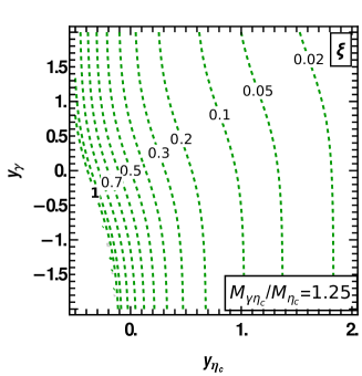
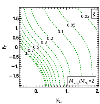
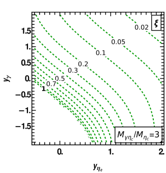
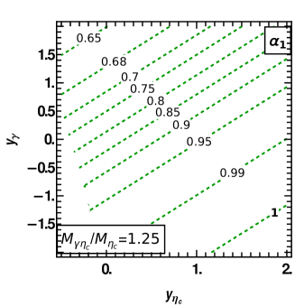
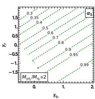
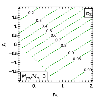
Figure 2: The contour plot illustrates the relation of the light-cone variable $\xi,\,\alpha_{1}\equiv\alpha_{\eta_{c}}$ with the rapidities of final state particles $y_{\eta_{c}},y_{\gamma}$ for different values of invariant mass $M_{\gamma\eta_{c}}$. For both particles we choose positive sign of rapidity for motion in direction of the incoming photon. For the sake of simplicity we consider the kinematics with zero transverse momenta of $\gamma,\eta_{c}$, which gives the dominant contribution in the total cross-section. The labels on contour lines show the values of $\xi,\,\alpha_{\eta_{c}}$.

In the generalized Bjorken kinematics, the variables $m_{N},\,\left|\Delta_{\perp}\right|,t$ are negligibly small, whereas all the other variables are parametrically large, $\sim M_{\eta_{c}}$. In this kinematics it is possible to simplify the light-cone decomposition (1-5) and obtain approximate relations of the Mandelstam variables with variables $\alpha_{\eta_{c}},\boldsymbol{p}_{\perp}$ as

$$-t^{\prime}\approx\alpha_{\eta_{c}}M_{\gamma\eta_{c}}^{2}-M_{\eta_{c}}^{2},\qquad-u^{\prime}\approx\left(1-\alpha_{\eta_{c}}\right)M_{\gamma\eta_{c}}^{2},\qquad\boldsymbol{p}_{\perp}^{2}=\alpha_{\eta_{c}}\left(1-\alpha_{\eta_{c}}\right)M_{\gamma\eta_{c}}^{2},\qquad M_{\gamma\eta_{c}}^{2}\approx 2s\xi$$ (12)

The physical constraint for real photon momenta

$$t^{\prime}=\left(q-k\right)^{2}=-2q\cdot k=-2\,\left|\boldsymbol{q}\right|\left|\boldsymbol{k}\right|\left(1-\cos\theta_{\boldsymbol{q},\,\boldsymbol{k}}\right)\leq 0,$$ (13)

implies that the variable $\alpha_{\eta_{c}}$ is bound by $\alpha_{\eta_{c}}\geq M_{\eta_{c}}^{2}/M_{\gamma\eta_{c}}^{2}$, so for the variable $u^{\prime}$ we get

$$-u^{\prime}\leq\left(-u^{\prime}\right)_{{\rm max}}=M_{\gamma\eta_{c}}^{2}-M_{\eta_{c}}^{2}-t.$$ (14)

We also may check that the pairwise invariant masses

$$\left(P_{{\rm out}}+p_{\eta_{c}}\right)^{2} \approx M_{\eta_{c}}^{2}+s\alpha_{\eta_{c}}\left(1-\xi\right)=t^{\prime}+s\alpha_{\eta_{c}},\qquad\left(P_{{\rm out}}+k\right)^{2}\approx s\left(1-\alpha_{\eta_{c}}\right)\left(1-\xi\right),$$

remain large, which shows that the produced $\eta_{c}$ and $\gamma$ are well-separated kinematically from the recoil proton.

In what follows we prefer to use as independent variables $t,t^{\prime},M_{\gamma\eta_{c}}$ since, as we will see below, the cross-section decreases homogeneously as a function of these variables. The photoproduction cross-section in terms of these variables may be represented as

$$\frac{d\sigma_{\gamma p\to\eta_{c}\gamma p}}{dt\,dt^{\prime}\,dM_{\gamma\eta_{c}}}\approx\frac{\left|\mathcal{A}_{\gamma p\to\eta_{c}\gamma p}\right|^{2}}{128\pi^{3}W^{4}M_{\gamma\eta_{c}}}$$ (15)

where $\mathcal{A}_{\gamma p\to\eta_{c}\gamma p}$ is the amplitude of the process. The electroproduction cross-section in the small-$Q$ kinematics gets the dominant contribution from events with single-photon exchange between leptonic and hadronic parts, and may be represented as Weizsacker:1934 ; Williams:1935 ; Budnev:1975poe

$$\frac{d\sigma_{ep\to eM_{1}M_{2}p}}{d\ln W^{2}dQ^{2}\,dt\,dt^{\prime}\,dM_{\gamma\eta_{c}}}\approx\frac{\alpha_{{\rm em}}}{\pi\,Q^{2}}\,\left(1-y+\frac{y^{2}}{2}-(1-y)\frac{Q_{{\rm min}}^{2}}{Q^{2}}\right)\frac{d\sigma_{\gamma p\to M_{1}M_{2}p}}{dt\,dt^{\prime}\,dM_{\gamma\eta_{c}}},$$ (16)

where $Q_{{\rm min}}^{2}=m_{e}^{2}y^{2}/\left(1-y\right)$, $m_{e}$ is the mass of the electron and $y$ is the fraction of the electron energy which passes to the virtual photon (the so-called inelasticity); it may be related to the invariant energy $\sqrt{s_{ep}}$ of the electron-proton collision as

$$y=\frac{W^{2}+Q^{2}-m_{N}^{2}}{s_{ep}-m_{N}^{2}}.$$ (17)

II.2 The amplitude of the $\eta_{c}\gamma$ pair production

In the chosen kinematics it is possible to evaluate the amplitude $\mathcal{A}_{\gamma p\to\eta_{c}\gamma p}$ in the collinear factorization framework, and express it in terms of the GPDs of the target Diehl:2000xz ; Diehl:2003ny ; Guidal:2013rya ; Boer:2011fh ; Burkert:2022hjz . As usual, we will disregard the mass of the proton $m_{N}$ and all components of the momentum transfer $\Delta^{\mu}$. Furthermore, we will assume that the invariant mass $M_{\gamma\eta_{c}}$ is large enough to exclude feed-down contributions from radiative decays of higher state charmonia. Our evaluation resembles previous evaluation of the gluonic coefficient function for $\gamma\pi^{0}$ GPD2x3:8 ; GPD2x3:9 ; Duplancic:2024opc ; Nabeebaccus:2023 , however due to use of heavy quark mass limit and NRQCD instead of pion wave function, the final result is materially different and does not allow direct comparison. In Appendix A we provide a more detailed evaluation, which takes into account the relative motion of heavy quarks in charmonia, and reduces to results of GPD2x3:8 ; GPD2x3:9 ; Duplancic:2024opc ; Nabeebaccus:2023 in hypothetical limit of vanishing quark mass.

Since the GPDs are defined in the so-called symmetric frame, for evaluation of the coefficient functions formally we should switch to that frame, applying a transverse Lorentz boost

$$\ell^{+} \to\ell^{+},\qquad\ell^{-}\to\ell^{-}+\ell^{+}\beta_{\perp}^{2}+\boldsymbol{\ell}_{\perp}\cdot\boldsymbol{\beta}_{\perp},\qquad\boldsymbol{\ell}_{\perp}\to\boldsymbol{\ell}_{\perp}+\ell^{+}\boldsymbol{\beta}_{\perp},\quad{\rm where}\quad\boldsymbol{\beta_{\perp}}=-\boldsymbol{\Delta_{\perp}}/\left(2\bar{P}_{{\rm SRF}}^{+}\right)$$ (18)

to the light-cone decomposition defined in (1-5). However, since the momentum $\boldsymbol{\Delta}_{\perp}$ eventually can be disregarded when evaluating the coefficient function, we will omit this step and will not distinguish the photon-proton  (1-5) and the symmetric frames. The evaluation of the partonic-level amplitude is straightforward. The momenta of the active parton (gluon) before and after interaction are given explicitly by

$$k_{i} =\left((x+\xi)\bar{P}^{+},\,0,\,0\right),\quad k_{f}=\left((x-\xi)\bar{P}^{+},\,0,\,\boldsymbol{\Delta}_{\perp}\right)$$ (19)

where $x$ is the light-cone fraction of average momentum $\left(k_{i}^{+}+k_{f}^{+}\right)2\bar{P}^{+}$. For unpolarized proton, the straightforward spinor algebra yields for the square of the amplitude Belitsky:2001ns

$$\sum_{{\rm spins}}\left|\mathcal{A}_{\gamma p\to M_{1}M_{2}p}\right|^{2} =\left[4\left(1-\xi^{2}\right)\left(\mathcal{H}_{\gamma\eta_{c}}\mathcal{H}_{\gamma\eta_{c}}^{*}+\tilde{\mathcal{H}}_{\gamma\eta_{c}}\tilde{\mathcal{H}}_{\gamma\eta_{c}}^{*}\right)-\xi^{2}\left(\mathcal{H}_{\gamma\eta_{c}}\mathcal{E}_{\gamma\eta_{c}}^{*}+\mathcal{E}_{\gamma\eta_{c}}\mathcal{H}_{\gamma\eta_{c}}^{*}+\tilde{\mathcal{H}}_{\gamma\eta_{c}}\tilde{\mathcal{E}}_{\gamma\eta_{c}}^{*}+\tilde{\mathcal{E}}_{\gamma\eta_{c}}\tilde{\mathcal{H}}_{\gamma\eta_{c}}^{*}\right)\right.$$ (20)

$$\qquad\left.-\left(\xi^{2}+\frac{t}{4m_{N}^{2}}\right)\mathcal{E}_{\gamma\eta_{c}}\mathcal{E}_{\gamma\eta_{c}}^{*}-\xi^{2}\frac{t}{4m_{N}^{2}}\tilde{\mathcal{E}}_{\gamma\eta_{c}}\tilde{\mathcal{E}}_{\gamma\eta_{c}}^{*}\right],$$

where, inspired by previous studies of Compton scattering and single-meson production Belitsky:2001ns ; Belitsky:2005qn , we introduced shorthand notations for the convolutions of the partonic amplitudes with GPDs

$$\mathcal{H}_{\gamma\eta_{c}}\left(\xi,\,t\right) =\int dx\,C_{\gamma\eta_{c}}\left(x,\,\xi\right)H_{g}\left(x,\xi,t\right),\qquad\mathcal{E}_{\gamma\eta_{c}}\left(y_{1},y_{2},t\right)=\int dx\,C_{\gamma\eta_{c}}\left(x,\,\xi\right)E_{g}\left(x,\xi,t\right),$$ (21)

$$\tilde{\mathcal{H}}_{\gamma\eta_{c}}\left(\xi,\,t\right) =\int dx\,\tilde{C}_{\gamma\eta_{c}}\left(x,\,\xi\right)\tilde{H}_{g}\left(x,\xi,t\right),\qquad\tilde{\mathcal{E}}_{\gamma\eta_{c}}\left(y_{1},y_{2},t\right)=\int dx\,\tilde{C}_{\gamma\eta_{c}}\left(x,\,\xi\right)\tilde{E}_{g}\left(x,\xi,t\right).$$ (22)

The partonic amplitudes $C_{\gamma\eta_{c}},\,\tilde{C}_{\gamma\eta_{c}}$ can be evaluated perturbatively, taking into account the diagrams shown in the Figure 3. In general the coefficient functions depend on polarization vectors of the incoming and outgoing photon. Since for the onshell photon there are only two polarizations, we may conclude that for the $\gamma p\to\eta_{c}\gamma p$ there are only two independent helicity amplitudes, without and with helicity flip. In what follows we will use additional superscript notations $C_{\gamma\eta_{c}}^{(++)}$ and $C_{\gamma\eta_{c}}^{(+-)}$ to distinguish them. The final result for the coefficient functions has a simple form (see Appendix A for details)

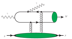
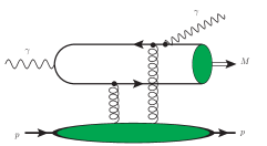
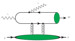
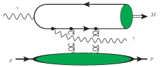
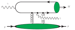
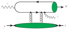
Figure 3: The diagrams which contribute to $\eta_{c}\gamma$ photoproduction. In all plots it is implied inclusion of diagrams which may be obtained by inversion of heavy quark lines (“charge conjugation”) and additional contribution of the diagrams with permuted gluon vertices in $t$-channel (24 diagrams in total, see Appendix A for more details).

$$C_{\gamma\eta_{c}}^{(++)} \left(r,\,\alpha,\,\zeta=x/\xi\right)=\frac{4\bar{\alpha}\mathfrak{C}_{\eta_{c}}}{\xi^{2}\alpha^{2}\left(1+\bar{\alpha}\right)^{2}\left(r^{2}-1\right)\left(\bar{\alpha}+1/r^{2}\right)}\times$$ (23)

$$\times\frac{1}{\left(\zeta+1-i0\right)\left(\zeta-1+i0\right)\left(\zeta+\kappa-i0\right)\left(\zeta-\kappa+i0\right)}\left[\frac{}{}\text{$\alpha$}^{2}\left(1+\bar{\alpha}\right)\left(\zeta^{2}+1\right)+\right.$$

$$+\frac{\left(\text{$\alpha$}^{2}-4\right)\zeta^{4}-2\left(\text{$\alpha$}^{3}-4\text{$\alpha$}+2\right)\zeta^{2}-\text{$\alpha$}\left(2\text{$\alpha$}^{2}+\text{$\alpha$}-4\right)}{\left(\zeta+1-i0\right)\left(\zeta-1+i0\right)r^{2}}+\frac{\left(1+\bar{\alpha}\right)^{2}\zeta^{4}+\text{$\alpha$}(\alpha^{2}+3\alpha-12)\zeta^{2}+\text{$\alpha$}(3\text{$\alpha$}^{2}+8\alpha-4)}{\left(\zeta+1-i0\right)\left(\zeta-1+i0\right)r^{4}}$$

$$+\frac{-\text{$\alpha$}\left((\text{$\alpha$}-4)\zeta^{2}+11\text{$\alpha$}+8\right)+8\zeta^{2}+4}{\left(\zeta+1-i0\right)\left(\zeta-1+i0\right)r^{6}}-\frac{4\left(\zeta^{2}-3\text{$\alpha$}\right)}{\left(\zeta+1-i0\right)\left(\zeta-1+i0\right)r^{8}}\left.-\frac{4}{\left(\zeta+1-i0\right)\left(\zeta-1+i0\right)r^{10}}\right]$$

$$C_{\gamma\eta_{c}}^{(+-)} \left(r,\,\alpha,\,\zeta=x/\xi\right)=\frac{4\mathfrak{C}_{\eta_{c}}}{\xi^{2}\alpha^{2}\left(1+\bar{\alpha}\right)^{2}\left(r^{2}-1\right)\left(\bar{\alpha}+1/r^{2}\right)\left(\zeta+1-i0\right)^{2}\left(\zeta-1+i0\right)^{2}\left(\zeta+\kappa-i0\right)\left(\zeta-\kappa+i0\right)}\times$$ (24)

$$\times\left[\frac{\alpha^{2}\left(3\alpha^{2}+\alpha-3\right)-2\bar{\alpha}\left(\alpha^{3}-4\alpha+2\right)\zeta^{2}-\left(1+\bar{\alpha}\right)^{2}\left(1-\alpha\bar{\alpha}\right)\zeta^{4}}{r^{2}}+\right.$$

$$-\frac{\alpha(3\alpha^{3}-2\alpha+5\alpha^{2}-8)-\bar{\alpha}\left(\alpha^{3}+3\alpha^{2}-8\right)\zeta^{2}+\bar{\alpha}\left(1+\bar{\alpha}\right)^{2}\zeta^{4}}{r^{4}}$$

$$+\frac{-\bar{\alpha}\alpha(\alpha+4)\zeta^{2}+\alpha(\alpha+3)(11\alpha-4)-4}{r^{6}}-\frac{4\left(3\alpha^{2}+7\alpha-2-\bar{\alpha}\zeta^{2}\right)}{r^{8}}\left.+\frac{4(\alpha+3)}{r^{10}}\right]$$

$$\tilde{C}_{\gamma\eta_{c}}^{(++)} \left(r,\,\alpha,\,\zeta=x/\xi\right)=-\frac{4\zeta\bar{\alpha}\mathfrak{C}_{\eta_{c}}}{\xi^{2}\alpha^{2}\left(1+\bar{\alpha}\right)^{2}\left(r^{2}-1\right)\left(\bar{\alpha}+1/r^{2}\right)}\times$$ (25)

$$\frac{1}{\left(\zeta+1-i0\right)\left(\zeta-1+i0\right)\left(\zeta+\kappa-i0\right)\left(\zeta-\kappa+i0\right)}\left[\frac{}{}2\alpha\left(1+\bar{\alpha}^{2}\right)+\right.$$

$$-\frac{2\left(\alpha^{3}-9\alpha^{2}+10\alpha-4+\left(2-5\bar{\alpha}-\bar{\alpha}^{3}\right)\zeta^{2}\right)}{\left(\zeta+1-i0\right)\left(\zeta-1+i0\right)r^{2}}-\frac{\left(3\alpha^{3}-17\alpha^{2}-8\alpha+16+\left(6-\bar{\alpha}-\bar{\alpha}^{3}\right)\zeta^{2}\right)}{\left(\zeta+1-i0\right)\left(\zeta-1+i0\right)r^{4}}$$

$$-\frac{\bar{\alpha}\left(3\alpha^{2}-40\alpha+16+\left(1+\bar{\alpha}\right)^{2}\zeta^{2}\right)}{\left(\zeta+1-i0\right)\left(\zeta-1+i0\right)r^{6}}-\frac{2(\alpha+5)}{\left(\zeta+1-i0\right)\left(\zeta-1+i0\right)r^{8}}\left.+\frac{4}{\left(\zeta+1-i0\right)\left(\zeta-1+i0\right)r^{10}}\right]$$

$$\tilde{C}_{\gamma\eta_{c}}^{(+-)} \left(r,\,\alpha,\,\zeta=x/\xi\right)=\frac{4\zeta\mathfrak{C}_{\eta_{c}}}{\xi^{2}\alpha^{2}\left(1+\bar{\alpha}\right)^{2}\left(r^{2}-1\right)\left(\bar{\alpha}+1/r^{2}\right)\left(\zeta+1-i0\right)^{2}\left(\zeta-1+i0\right)^{2}\left(\zeta+\kappa-i0\right)\left(\zeta-\kappa+i0\right)}\times$$ (26)

$$\times\left[\frac{2\alpha\left(-2\alpha^{2}-\alpha+2+(2\alpha^{3}-8\alpha^{2}+11\alpha-4)\zeta^{2}\right)}{r^{2}}-\frac{\alpha\left(3\alpha^{3}-16\alpha^{2}-7\alpha+8\right)+\left(\alpha^{4}-9\alpha^{2}+16\alpha-4\right)\zeta^{2}}{r^{4}}+\right.$$

$$+\frac{\alpha(3\alpha^{2}-35\alpha+8)-\bar{\alpha}\left(1+\bar{\alpha}\right)^{2}\zeta^{2}}{r^{6}}+\frac{4\left(\alpha^{2}+4\alpha-1\right)}{r^{8}}\left.+\frac{4\bar{\alpha}}{r^{10}}\right]$$

where we introduced shorthand notations $\alpha\equiv\alpha_{\eta_{c}}=(-u^{\prime})/M_{\gamma\eta_{c}}$, $\zeta=x/\xi$, the constant $\mathfrak{C}_{\eta_{c}}$ in the prefactors of (23-26) is given explicitly by

$$\mathfrak{C}_{\eta_{c}}=\frac{4}{9N_{c}m_{c}}\pi^{2}\alpha_{{\rm em}}\alpha_{s}\left(\mu\right)\sqrt{\left\langle\mathcal{O}_{\eta_{c}}\right\rangle/m_{c}^{3}},$$ (27)

$\left\langle\mathcal{O}_{\eta_{c}}\right\rangle\equiv\left\langle\mathcal{O}_{\eta_{c}}\left[{}^{1}S_{0}^{[1]}\right]\right\rangle\approx 0.3\,{\rm GeV^{3}}$ is the color singlet long-distance matrix element (LDME) of $\eta_{c}$ Braaten:2002fi , and $r$ is defined as

$$r=M_{\gamma\eta_{c}}/M_{\eta_{c}}=\frac{W}{M_{\eta_{c}}}\sqrt{\frac{2\xi}{1+\xi}\left(1-\frac{m_{N}^{2}}{W^{2}}\right)}\approx\frac{W}{M_{\eta_{c}}}\sqrt{\frac{2\xi}{1+\xi}}$$ (28)

We also may observe that at large $r$ the photon helicity flip components $C_{\gamma\eta_{c}}^{(+-)},\tilde{C}_{\gamma\eta_{c}}^{(+-)}$ have a relative suppression by factor $1/r^{2}$ compared to non-flip components $C_{\gamma\eta_{c}}^{(++)},\tilde{C}_{\gamma\eta_{c}}^{(+-)}$. This implies a strong suppression of these components in the high energy limit. The shorthand notation $\kappa$ which appears in the denominators of the first lines of (23-26) is defined as

$$\kappa=1-\frac{1-1/r^{2}}{1-\alpha/2}=\frac{1}{r^{2}}\frac{2-\alpha r^{2}}{2-\alpha}.$$ (29)

It is possible to check that in physically relevant kinematics ($r>1,\,\alpha\in(0,1)$) its values are limited by $|\kappa|<1$. The coefficient functions (23-26) have poles in ERBL region at $\zeta=\pm 1\mp i0$ and $\zeta=\pm\kappa\mp i0$ ($x=\pm\xi\mp i0$ and $x=\pm\kappa\xi\mp i0$ in conventional notations). The contour deformation prescription near these poles was found from conventional $m^{2}\to m^{2}-i0$ prescription in Feynman propagators. Some terms in (23-26) include ordinary second order poles $1/\left(x\mp\xi\pm i0\right)^{2}$, however they do not present any difficulties for convergence of integral: formally, the integration in the vicinity of these poles can be carried out using an identity

$$\int_{-1}^{1}dx\frac{F\left(x,\xi,t\right)}{\left(x-\xi+i0\right)^{2}} =-\int_{-1}^{1}dx\,F\left(x,\xi,t\right)\frac{d}{dx}\frac{1}{\left(x-\xi+i0\right)}=-\left.\frac{F\left(x,\xi,t\right)}{\left(x-\xi+i0\right)}\right|_{x=-1}^{x=+1}+\int_{-1}^{1}dx\,\frac{\partial_{x}F\left(x,\xi,t\right)}{\left(x-\xi+i0\right)}.$$ (30)

In the Figure 4 we show the density plot which illustrates the behavior of $C_{\gamma\eta_{c}}^{(++)}$ as a function of its arguments. We can see that the function is strongly concentrated in the vicinity of its poles, and decreases rapidly when we move away from them. This implies that position of the poles determines the region which gives the dominant contribution in convolution integrals (21-22). Varying the invariant mass $M_{\gamma\eta_{c}}$ and the value of $\alpha_{\eta_{c}}$, it is possible to change the parameter $\kappa$ in the region $|\kappa|<1$ and in this way probe the behavior of the gluon GPDs $H_{g}$ in the whole ERBL kinematics.

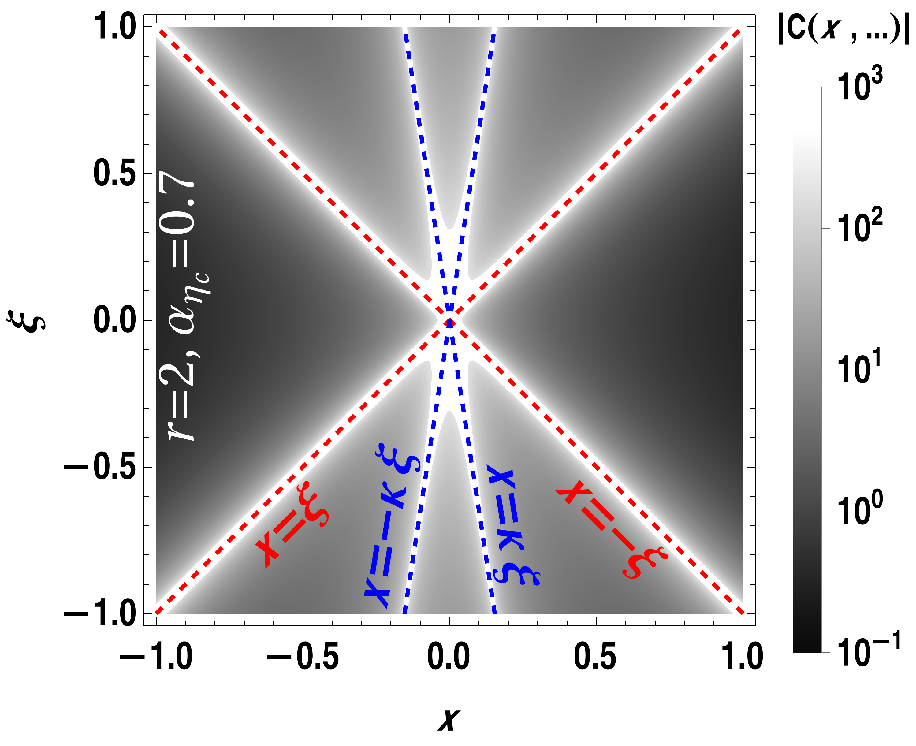
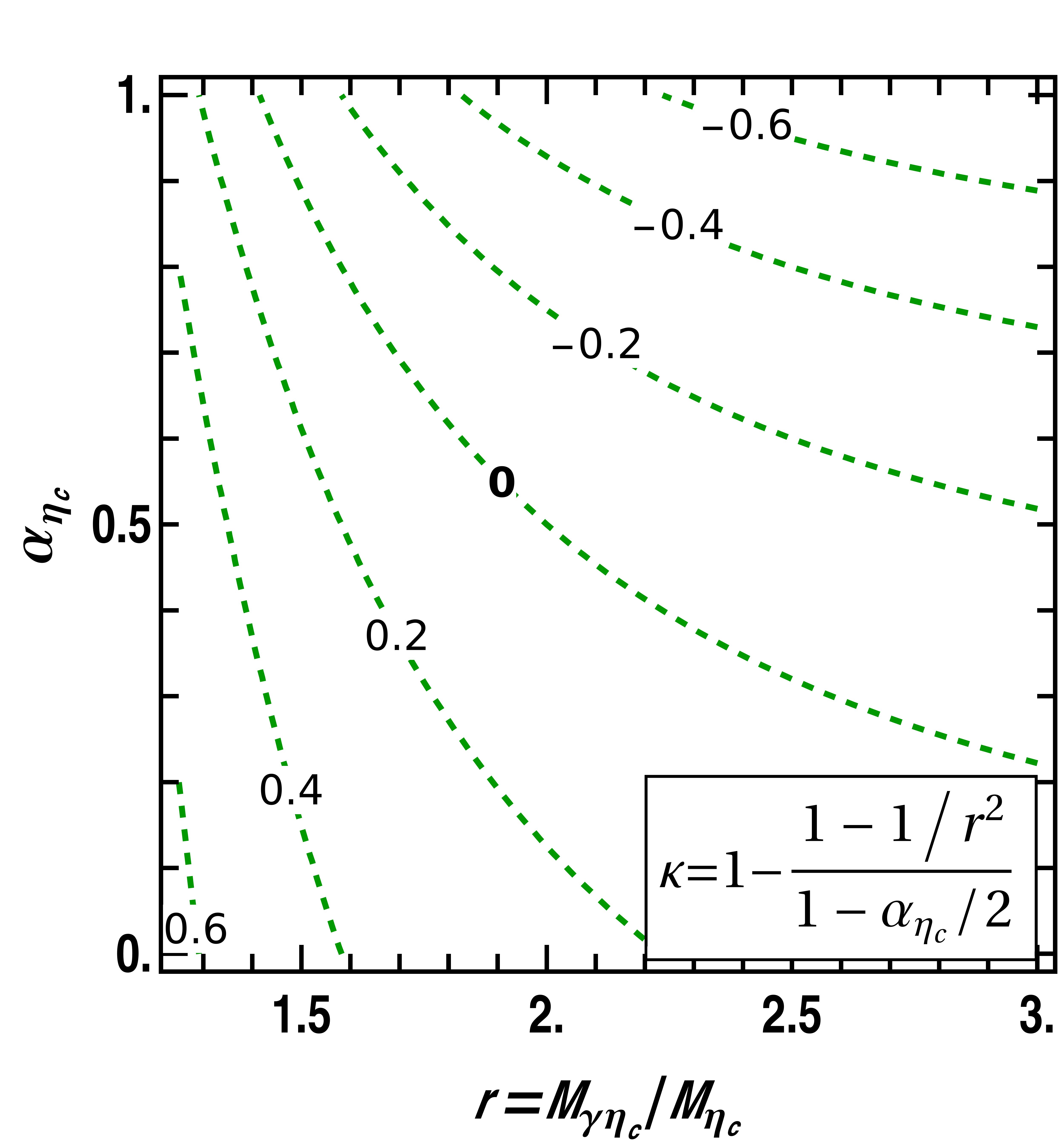
Figure 4: Left: Density plot which illustrates the coefficient function $C_{\gamma\eta_{c}}^{(++)}$ (in relative units) as a function of variables $x,\,\xi$. White lines effectively demonstrate the position of the poles $x=\pm\xi,\,x=\pm\kappa\,\xi$ in the coefficient function (23). The value of the slope parameter $\kappa$ depends on kinematics and is defined in (29). Right: Contour plot which shows the dependence of the slope parameter $\kappa$ on the choice of the kinematic variables $r=M_{\gamma\eta_{c}}/M_{\eta_{c}}$, $\alpha_{\eta_{c}}=(-u^{\prime})/M_{\gamma\eta_{c}}$. The parameter $\kappa$ is always is bound by a constraint $|\kappa|<1$ in the physically relevant kinematics.

III Numerical estimates

III.1 Differential cross-sections

In what follows for the sake of definiteness, we will use for our estimates the Kroll-Goloskokov parametrization of the GPDs Goloskokov:2006hr ; Goloskokov:2007nt ; Goloskokov:2008ib ; Goloskokov:2009ia ; Goloskokov:2011rd . As could be seen from (15,20), the cross-section of the process includes contributions of GPDs with different helicity states, however for unpolarized target the dominant contributions stems from the GPD $H^{g}\left(x,\xi,t\right)$.

We would like to start presentation of the results with discussion of the threefold differential cross-section (15) and its dependence on the invariant momentum transfer $t$ to the target. In the collinear kinematics the variable $|t|$ is small and is disregarded when evaluating the coefficient functions, for this reason the dependence of the cross-section on this variable is largely due to the implemented gluon GPD. In the Figure 5 we show this dependence for several invariant masses $M_{\gamma\eta_{c}}$ and choices of the variable $t^{\prime}$. A sharply decreasing $t$-dependence is common to many phenomenological parametrizations of the GPDs and was introduced to describe the pronounced $t$-dependence seen in DVCS and DVMP data. For the $\eta_{c}\gamma$ photoproduction this implies that photon and $\eta_{c}$ predominantly are produced with oppositely directed transverse momenta $\boldsymbol{p}_{\eta_{c}}^{\perp},\,\boldsymbol{p}_{\gamma}^{\perp}$. In view of a simple and well-understood dependence on $t$, in what follows we will tacitly assume that $|t|=|t_{{\rm min}}|$, or consider the observables in which the dependence on $t$ is integrated out.

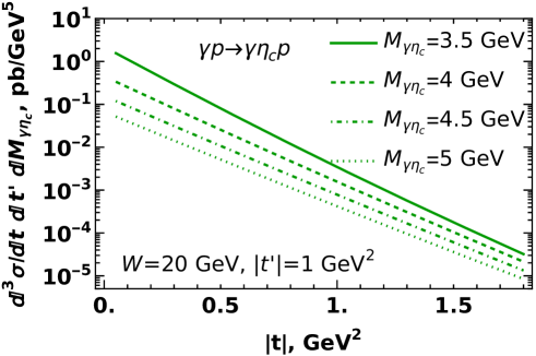
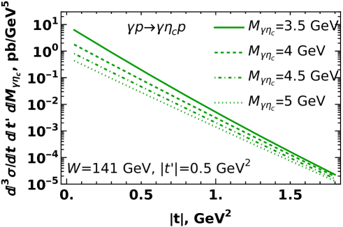
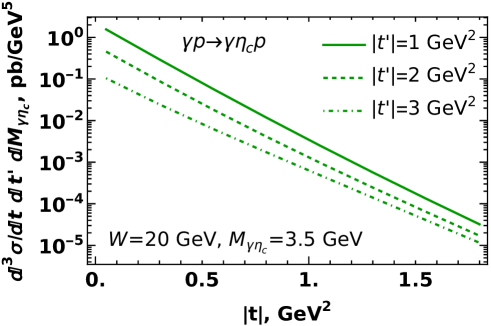
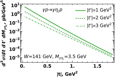
Figure 5: Dependence of the photoproduction cross-section (15) on the invariant momentum transfer $t$ to the target at fixed invariant mass $M_{\gamma\eta_{c}}$ (upper row) and fixed $|t^{\prime}|$ (lower row). The left and right columns differ by value of invariant energy $W$. For other energies, the $t$-dependence has similar shape.

In the Figure 6 we show the dependence of the cross-section (15) on the variable $\left|t^{\prime}\right|$. Similar to the previous case, the cross-section decreases rapidly as a function of this variable. As could be seen from (12), the dependence on $|t^{\prime}|$ at fixed invariant mass $M_{\gamma\eta_{c}}^{2}$ is unambiguously related to $\alpha_{\eta_{c}}$-dependence of the coefficient functions (23-26). The pefactor $\sim 1/\alpha_{\eta_{c}}^{2}$ which appears in front of all coefficient functions is partially responsible for the observed $t^{\prime}$-dependence of the cross-section.

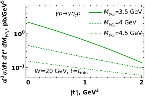
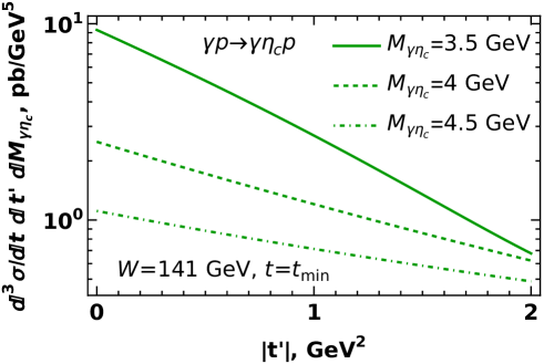
Figure 6: Dependence of the photoproduction cross-section (15) on the variable $|t^{\prime}|$ defined in  (15). The left and right plot correspond to different invariant energies $W=20$ GeV and $W=141$ GeV respectively.

In the Figure 7 we show the dependence of the cross-section on the invariant energy $W$. As expected, the cross-section grows with $W$, and nearly linear dependence in double logarithmic coordinates suggests that the cross-section has a power-like dependence on energy, $d\sigma(W)\sim W^{\lambda}$, where the parameter $\lambda$ has a mild dependence on other kinematic variables. This behavior may be understood if we take into account that the amplitude gets the dominant contribution from the gluon GPD near $|x|\sim\xi\sim 1/W^{2}$, and the fact that the gluon GPDs grows as a function of the light-cone fraction $x$. In the implemented phenomenological parametrization, the small-$x$ behavior of the GPD roughly may be approximated as $H_{g}(x,\xi,t)\sim x^{-\delta_{g}}$ Goloskokov:2006hr . After convolution with coefficient functions (23-26), this translates into a power-like behavior for the cross-section,

$$\frac{d\sigma(W)}{dt\,dt^{\prime}\,dM_{\gamma\eta_{c}}}\sim\xi^{-2\delta_{g}}\sim W^{4\delta_{g}},\qquad\lambda=4\delta_{g},$$ (31)

in agreement with results of numerical evaluation. The typical values of the parameter $\lambda$ are $\lambda\approx 0.7-0.8$.

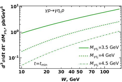
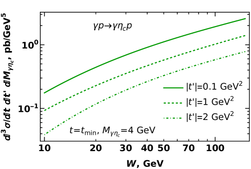
Figure 7: Dependence of the cross-section on the invariant collision energy $W$ at different values of the invariant mass $M_{\gamma\eta_{c}}$ (left) and variable $|t^{\prime}|$ (right). The energy dependence of the cross-section may be approximated as $d\sigma(W)/dt\,dt^{\prime}\,dM_{\gamma\eta_{c}}\sim W^{\lambda}$, where the slope parameter $\lambda$ has a very mild dependence on other kinematic variables.

In the Figure 8 we show the dependence of the cross-section on the invariant mass $M_{\gamma\eta_{c}}$. The dependence is very pronounced and is a consequence of prefactor $\sim 1/\left(r^{2}-1\right)=M_{\eta_{c}}^{2}/\left(M_{\gamma\eta_{c}}^{2}-M_{\eta_{c}}^{2}\right)$ in coefficient functions  (23-26) and additional factor $\sim 1/M_{\gamma\eta_{c}}$ in the cross-section (15). Similar dependence on invariant mass was also observed in other photon-meson production channels in the kinematics where invariant mass is large.

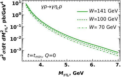
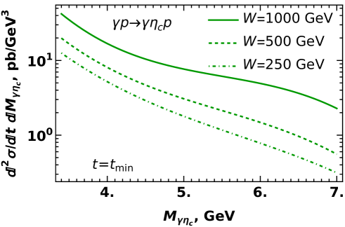
Figure 8: Dependence of the cross-section on the invariant masses of produced $\gamma\eta_{c}$ pair, for several proton energies in the kinematics of EIC (left) and ultraperipheral collisions at LHC (right). The right plot should be considered only as order of magnitude estimate due to possible NLO corrections and saturation effects.

Finally, we would like to discuss the relative contribution of different polarizations of the final state photon to the total cross-section. In the Figure 9 we plotted the ratio of the cross-sections with and without the helicity flip of the final-state photon. As expected, the ratio decreases as a function of energy $W$, though its dependence on variables $|t|$ and $M_{\gamma\eta_{c}}$ is more complicated and depends on the implemented parametrization of the GPD. However, we can see that the ratio remains small (a few per cent or below) in the region of small $|t|,\,M_{\gamma\eta_{c}}$ where the cross-section is sufficiently large for experimental studies, and for this reason predominantly the final-state and incoming photons will have the same polarization.

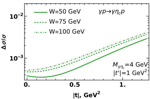
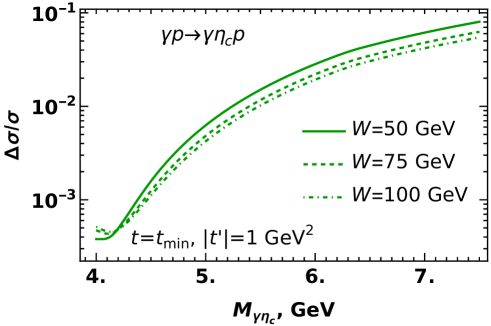
Figure 9: The ratio of the cross-sections with and without photon helicity flip, as a function of the momentum transfer $|t|$ to the target and invariant mass of the $\eta_{c}\gamma$ pair. The ratio remains small (below 10%) in the whole range analyzed in this paper.

III.2 Integrated cross-sections and counting rates

So far we considered the differential cross-sections, which are best suited for theoretical studies. Unfortunately, it is difficult to measure such small cross-sections because of insufficient statistics, and for this reason now we will provide predictions for the yields integrated over some or all kinematic variables. In the left panel of the Figure 10 we have shown the cross-section $d\sigma/dM_{\gamma\eta_{c}}$ for different energies. For the sake of comparison we also added a colored band which corresponds to cross-section of $\gamma p\to\gamma\pi^{+}n$ at $W=14$ GeV found in GPD2x3:9  . The width of the band represents uncertainty due to choice of pion distribution amplitudes and quark GPDs. We may see that the cross-sections of $\eta_{c}\gamma$ and $\pi^{-}\gamma$ photoproduction have similar magnitudes if compared at the same (large) values of the invariant mass of photon-meson pair.

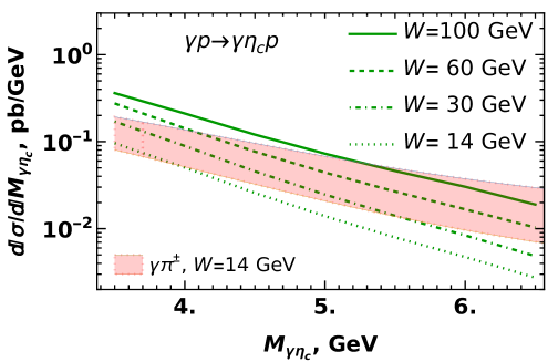
Figure 10: The single-differential cross-section $d\sigma/dM_{\gamma\eta_{c}}$ as a function of the invariant mass of $\eta_{c}\gamma$ pair at different collision energies. For reference we also added the colored band which corresponds to the cross-section of $\gamma p\to\gamma\pi^{+}n$ at $W=14$ GeV found in GPD2x3:9 .

In the left panel of the Figure 11 we show the energy dependence of the total (fully integrated) cross-section $\sigma_{{\rm tot}}(W)$ for the photoproduction of $\eta_{c}\gamma$. As we discussed earlier, the suggested mechanism may be applied only in the kinematics where the invariant mass $M_{\gamma\eta_{c}}$ of the photon-meson pair is sufficiently large in order to avoid the feed-down contributions from radiative decays of the excited quarkonia states. The choice of the minimal value $\left(M_{\gamma\eta_{c}}\right)_{{\rm min}}$ is somewhat arbitrary, for this reason we have shown the result for several possible cutoffs. This dependence is stronger at small energies due to phase space contraction for production of $\eta_{c}\gamma$ pair with large invariant mass. At large $W$, for all cutoffs the $W$-dependence may be approximated as

$$\sigma_{{\rm tot}}\left(W,\,M_{\gamma\eta_{c}}\geq 3.5\,{\rm GeV}\right)\approx 0.48\,{\rm pb}\,\left(\frac{W}{100\,{\rm GeV}}\right)^{0.75},$$ (32)

in agreement with our earlier findings (31) for the energy dependence of the differential cross-sections. In the right panel of the same Figure 11 we have shown our estimates for the fully integrated cross-section of the electroproduction $ep\to e\gamma\eta_{c}p$ as a function of the invariant electron-proton collision energy $\sqrt{s_{ep}}$. For the upper EIC energy $\sqrt{s_{ep}}\approx 141\,$GeV the corresponding cross-section is

$$\sigma_{{\rm tot}}^{({\rm ep})}\left(\sqrt{s_{ep}}=141\,{\rm GeV},\,M_{\gamma\eta_{c}}\geq 3.5\,{\rm GeV}\right)\approx 49\,{\rm fb}.$$ (33)

This smallness is due to $\sim\alpha_{{\rm em}}$ in the leptonic prefactor (see (16)) and a very steep slope of the $t$-dependence in the exclusive process. For the instantaneous luminosity $\mathcal{L}=10^{34}\,{\rm cm^{-2}s^{-1}}=10^{-5}{\rm fb}^{-1}s^{-1}$ at the future Electron Ion Collider Accardi:2012qut ; AbdulKhalek:2021gbh ; Navas:2024X the cross-section (33) gives a production rate $dN/dt\approx$42 events/day, with approximately $N=4.9\times 10^{3}$ produced $\eta_{c}\gamma$ pairs per each $\int dt\,\mathcal{L}=100{\rm fb^{-1}}$ of integrated luminosity. Since $\eta_{c}$ mesons are not detected directly but rather via their decays into light hadrons, for analysis of feasibility it is also interesting to know the counting rate $dN_{d}/dt$ and the total number of detected events $N_{d}$ for a chosen decay mode. Technically, these quantities may be found multiplying $dN/dt$ and $N$ by the branching fraction of $\eta_{c}$ to the chosen decay mode. In experimental studies the $\eta_{c}$-meson is frequently identified via its decays to pions and kaons, e.g.: $\eta_{c}(1S)\to K_{S}^{0}K^{+}\pi^{-}$, for which the corresponding branching fraction is BESIII:2019eyx ; Navas:2024X

$${\rm Br}_{\eta_{c}}={\rm Br}\left(\eta_{c}(1S)\to K_{S}^{0}K^{+}\pi^{-}\right)=2.6\%.$$ (34)

This translates into detection (counting) rate $dN_{d}/dt\approx$32 events/month, with $N_{d}=$127 detected events per $100{\rm fb^{-1}}$ of integrated luminosity.

For the kinematics of the ultraperipheral collisions at LHC, the counting rates could be significantly larger due to increase of the cross-section with energy. Furthermore, in $pA$ collisions the counting rate could be additionally enhanced by factor $\sim Z^{2}$ in the photon flux, where $Z$ is the atomic number of the projectile nucleus. However, the suggested approach might be not applicable in that kinematics due to onset of saturation effects, so we abstain from making detailed predictions for LHC energies.

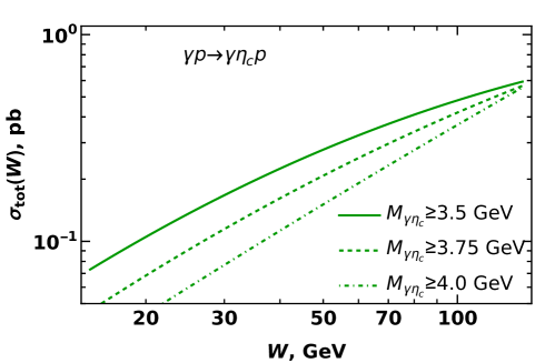
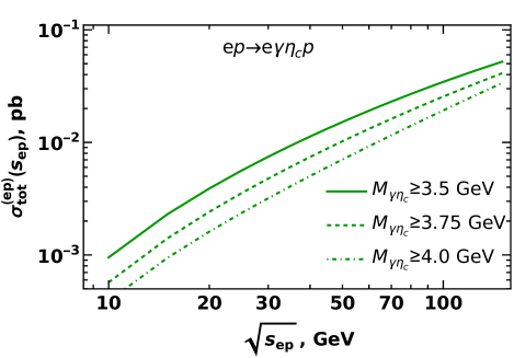
Figure 11: Predictions for the total (“fiducial”) cross-section of photoproduction (left) and electroproduction (right) of $\eta_{c}\gamma$ as a function of energy $W$ for different cutoffs on the invariant mass of $\eta_{c}\gamma$ pairs.

III.3 Comparison with $\eta_{c}$ photoproduction

The exclusive $\eta_{c}$ photoproduction process $\gamma p\to\eta_{c}p$ for a long time has been considered as one of the most promising channels for studies of odderons Odd4 ; Odd5 ; Odd6 ; Odd7 : the $C$-odd 3-gluon exchanges in $t$-channel predicted in Odd1 ; Odd2 ; Odd3 . While the existence of the odderons has never been questioned, for a long time the magnitude of the odderon-mediated processes remained largely unknown because it is controlled by a completely new nonperturbative amplitude (see Odd7 ; Benic:2023 for a short overview). Only recently the experimental measurements could confirm nonzero contribution of odderons from comparison of $pp$ and $p\bar{p}$ elastic cross-sections measured at LHC and Tevatron OddTotem1 ; OddTotem2 . Since that analysis potentially could include sizable uncertainties due to details of extrapolation procedure, the searches of odderons shifted towards channels which require the $C$-odd $t$-channel exchanges. The photoproduction $\gamma p\to\eta_{c}p$ is a rather clean channel for study of odderons using perturbative methods, and for this reason it will remain in focus of future experimental studies, both at HL-LHC and at future EIC.

The $\eta_{c}\gamma$ photoproduction in this context deserves a lot of interest because it could constitute a sizable background to $\eta_{c}$ photoproduction. Indeed, the $\eta_{c}\gamma$ photoproduction does not require small $C$-odd exhanges in $t$-channel, and the latter fact potentially could compensate the expected $\mathcal{O}\left(\alpha_{{\rm em}}\right)$-suppression of the cross-section. Since the acceptance of modern detectors for photons is below unity, potentially the $\eta_{c}\gamma$ photoproduction with undetected final-state photons could be misinterpreted as $\gamma p\to\eta_{c}p$ subprocess. The accurate estimate of the background in general requires detailed knowledge of the detector’s geometry and acceptance. For the sake of simplicity we will assume that all photons are undetected, and will discuss the cross-section $d\sigma/dt$, integrating over the phase space of the produced photon. Such approach provides an upper estimate for the background.

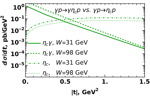
Figure 12: Comparison of the cross-sections of the $\gamma p\to\eta_{c}p$ and $\gamma p\to\eta_{c}\gamma p$ with undetected (integrated out) final-state photon. The cross-section of $\gamma p\to\eta_{c}p$ is taken from Odd7 ; Benic:2023 (curves $x=10^{-2}$ and $x=10^{-3}$, the values of $W$ are restored assuming the relation $x=M_{\eta_{c}}^{2}/W^{2}$).

In the Figure (12) we compare the cross-sections of the $\eta_{c}$ and $\eta_{c}\gamma$ with undetected (integrated out) photon in the final state. We can see that in the small-$t$ kinematics ($|t|\lesssim 0.5\,{\rm GeV}^{2}$) the cross-section of $\eta_{c}\gamma$ exceeds the cross-section of the $\eta_{c}$ photoproduction, though becomes suppressed exponentially at higher $t$ due to implemented GPD model Goloskokov:2006hr ; Goloskokov:2007nt ; Goloskokov:2008ib ; Goloskokov:2009ia ; Goloskokov:2011rd . Furthermore, the cross-section of $\eta_{c}\gamma$ grows faster with energy and thus eventually will exceed the $\eta_{c}$ cross-section at any $t$. In collinear factorization approach the energy dependence is controlled by $x$-dependence of the GPD parametrization. In BFKL language, the difference of energy dependencies of $\eta_{c}\gamma$ and $\eta_{c}$ is a consequence of the fact that pomeron has larger intercept than odderon.

The fact that the odderon contribution in the small-$t$ kinematics can be shadowed by other mechanisms has been discussed earlier in Benic:2023 . However, the corrections discussed in that paper depend on the isospin of the target, and are significantly less important for processes on neutrons, namely for $\gamma n\to\eta_{c}n$ subprocess. In contrast, the cross-section of $\eta_{c}\gamma$ does not depend on isospin of the target and will be the same for $\gamma n\to\eta_{c}\gamma n$ and $\gamma p\to\eta_{c}\gamma p$ subprocesses.

IV Conclusions

In this paper we analyzed the exclusive $\eta_{c}\gamma$ photoproduction in the collinear factorization approach. Our evaluation in the massless limit agrees with earlier evaluations of the gluonic coefficient function for $\gamma\pi^{0}$ photoproduction GPD2x3:8 ; GPD2x3:9 . The nonzero quark mass allows to avoid factorization breaking pinch singularities which were discovered in Duplancic:2024opc ; Nabeebaccus:2023 in massless case. The coefficient function of the process is given by a simple meromorphic function of its arguments, with two “classical” poles at $x=\pm\xi$, and two additional poles at $x=\pm\kappa\,\xi$, where the value of $\kappa$ depends on kinematics (values of $M_{\gamma\eta_{c}}$ and $u^{\prime}$) and is bound by $|\kappa|<1$ in the physically permitted kinematical range. The analytic structure of the coefficient function apparently does not allow deconvolution (direct extraction of GPDs from amplitudes). However, we observed that the coefficient function is strongly peaked in the vicinity of its poles, and falls off rapidly outside, so the cross-section of the process is largely determined by the behavior of the gluon GPDs near these poles. Varying the kinematics and in this way changing position of the poles, the suggested process may be used to constrain the existing phenomenological parametrizations of GPDs in the whole ERBL region.

Numerically, the amplitude of the process obtains the dominant contribution from the unpolarized gluon GPD $H_{g}$ in ERBL kinematics. The cross-section of $\eta_{c}\gamma$ photoproduction is comparable to cross-sections of the process $\gamma^{*}p\to\gamma Mp$, $M=\pi,\,\rho$ if we compare them at the same (large) values of invariant masses of meson-photon pair. However, due to inherently large value of the invariant mass of the $\gamma\eta_{c}$ pair, the total (integrated) photoproduction cross-section is below a picobarn. Nevertheless, we expect that this cross-section is within the reach of experimental studies: for example, for $ep$ collisions at EIC we estimate the production rate of a few thousand $\eta_{c}\gamma$ pairs per each 100 ${\rm fb}^{-1}$ of integrated luminosity. We observed that the cross-section grows with energy and could reach large values for TeV-range photon-proton collisions, however in that kinematics the suggested approach is not very reliable due to expected large NLO corrections and onset of saturation effects.

We expect that the suggested process could be studied in ultraperipheral collisions at LHC, as well as in electron-proton collisions at the future Electron Ion Collider (EIC) Accardi:2012qut ; AbdulKhalek:2021gbh ; Burkert:2022hjz and possibly at JLAB after future 22 GeV upgrade Accardi:2023chb .

Acknowldgements

We thank our colleagues at UTFSM university for encouraging discussions. We also thank M. Sanhueza for providing links to references Odd7 ; Benic:2023 . This research was partially supported by ANID PIA/APOYO AFB230003 (Chile) and Fondecyt (Chile) grant 1220242. "Powered@NLHPC: This research was partially supported by the supercomputing infrastructure of the NLHPC (ECM-02)".

Appendix A Evaluation of the coefficient functions

The evaluation of the coefficient functions can be performed using the standard light–cone rules from Lepage:1980fj ; Brodsky:1997de ; Diehl:2000xz ; Diehl:2003ny ; Diehl:1999cg ; Ji:1998pc . As discussed in Section II.1, we disregard the proton mass $m_{N}$ and the invariant momentum transfer to the proton $t=\Delta^{2}$, treating all the other variables as parametrically large quantities of order $m_{c}$. The evaluation of the partonic amplitudes shown in the Figure 3 is straightforward.

In order to compare our results with earlier papers on $\gamma\pi^{0}$ production, we will assume that the heavy quarks carry the fractions $z$ and $1-z$ of the quark-antiquark momenta, though eventually we will disregard the internal motion of the quarks inside $\eta_{c}$ and take the limit $z=1/2$. Formally, this can be done introducing the light-cone distribution amplitude (LCDA), and relating it to NRQCD LDMEs, as discussed in Ma:2006hc ; Wang:2013ywc ; Wang:2017bgv . The definitions of quarkonia distribution amplitude is a straightforward extensions of general results formulated for light mesons LightQuarkDA:1 ; LightQuarkDA:2 ; LightQuarkDA:3 ; LightQuarkDA:4 ; LightQuarkDA:5 . For the spinless $\eta_{c}$-meson, at leading twist there is only one distribution amplitude defined as

$$\Phi_{\eta_{c}}\left(z\right) =\int\frac{d\lambda}{2\pi}e^{izp^{+}\lambda}\left\langle 0\left|\bar{\psi}\left(-\frac{\lambda}{2}\right)\gamma^{+}\gamma_{5}\mathcal{L}\left(-\frac{\lambda}{2},\,\frac{\lambda}{2}\right)\psi\left(\frac{\lambda}{2}\right)\right|\eta_{c}(p)\right\rangle,$$ (35)

$$\mathcal{L}\left(-\frac{\lambda}{2},\,\frac{\lambda}{2}\right)\equiv\mathcal{P}{\rm exp}\left(i\int_{-\lambda/2}^{\lambda/2}d\zeta\,A^{+}\left(\zeta\right)\right).$$ (36)

where we assume that $\eta_{c}$ moves in the plus-direction, $z$ is the fraction of its momentum carried by the $c$-quark, $\mathcal{L}$ is the usual Wilson link. Sometimes the definition (35) is written for the distribution amplitudes normalized to unity and thus may include additional normalization factor (decay constant $f_{\eta_{c}}$). The NRQCD approach constructs the description of quarkonia states in terms of long-distance matrix elements with structure $\left\langle 0\left|\hat{\mathcal{O}}\right|\eta_{c}(p)\right\rangle,$ where $\hat{\mathcal{O}}$ is a set of local operators built from operators of quarks, antiquarks and their covariant derivatives. The relation of the two approaches has been discussed in detail in Ma:2006hc ; Wang:2013ywc ; Wang:2017bgv . The distribution amplitudes may be expressed in terms of NRQCD LDMEs as

$$\Phi_{\eta_{c}}(z)=\hat{\Phi}_{\eta_{c}}\left(z\right)\frac{\left\langle 0\left|\hat{\mathcal{O}}_{\eta_{c}}\right|\eta_{c}(p)\right\rangle}{2\sqrt{m_{c}}}\left(1+\mathcal{O}\left(v^{2}\right)\right),$$ (37)

where $\hat{\Phi}\left(z\right)$ is the perturbative (partonic-level) distribution amplitude, and the denominator is conventionally added to take into account the difference between normalizations of Fock states used in LCDA and NRQCD pictures. In the leading order over relative velocity $v\sim\mathcal{O}\left(\alpha_{s}\left(m_{c}\right)\right)$ the distribution amplitude may be written as

$$\hat{\Phi}_{\eta_{c}}\left(z\right)\sim f_{\eta_{c}}\delta\left(z-\frac{1}{2}\right)+\mathcal{O}\left(v^{2}\right).$$ (38)

As was discussed in Ma:2006hc , the next-to-leading order corrections to the amplitude (38) give nontrivial dependence on $z$, however we will eventually disregard it, since formally it is a higher-order correction in $\alpha_{s}$. Conversely, the color singlet LDMEs $\left\langle 0\left|\hat{\mathcal{O}}_{\eta_{c}}\right|\eta_{c}(p)\right\rangle$ may be expressed in terms of the moments of the distribution amplitude $\Phi_{\eta_{c}}(z)$.

In general, the coefficient functions $C_{\mathfrak{\gamma\eta_{c}}},\,\tilde{C}_{\mathfrak{\gamma\eta_{c}}}$ which appear in (21-22) should be understood as convolutions of partonic-level amplitudes with distribution amplitudes $\Phi_{\eta_{c}}$, namely,

$$C_{\mathfrak{\gamma\eta_{c}}}\left(x,\,\xi\right) =\int_{0}^{1}\,dz\,c\left(x,\,\xi,\,z\right)\Phi_{\eta_{c}}\left(z\right),\qquad\tilde{C}_{\gamma\eta_{c}}\left(x,\,\xi\right)=\int_{0}^{1}\,dz\,\tilde{c}\left(x,\,\xi,\,z\right)\Phi_{\eta_{c}}\left(z\right).$$ (39)

The evaluation of the partonic amplitudes $c\left(x,\,\xi,\,z\right),\,\tilde{c}\left(x,\,\xi,\,z\right)$ may be done perturbatively. The projections onto a state with total spin $S=0$ in the NRQCD picture may be found using proper Clebsch-Gordan coefficients Cho:1995ce ; Cho:1995vh ; DVMPcc1 ,

$$\hat{P}_{SS_{z}}^{ij} =-\sqrt{\frac{\left\langle\mathcal{O}_{\eta_{c}}\right\rangle}{m_{Q}}}\,\frac{1}{8m_{Q}}\left(\frac{\hat{p}_{\eta_{c}}}{2}-\frac{\hat{\delta}_{\eta_{c}}}{2}-m_{c}\right)\gamma_{5}\left(\frac{\hat{p}_{\eta_{c}}}{2}+\frac{\hat{\delta}_{\eta_{c}}}{2}+m_{c}\right)\otimes\frac{\delta_{ij}}{\sqrt{N_{c}}},$$ (40)

where $\left\langle\mathcal{O}_{\eta_{c}}\right\rangle\equiv\left\langle\mathcal{\mathcal{O}}_{\eta_{c}}^{[1]}\left({}^{1}S_{0}^{[1]}\right)\right\rangle\approx 0.3\,{\rm GeV^{3}}$ is the dominant color singlet LDME of $\eta_{c}$ meson Braaten:2002fi , $\delta_{\eta_{c}}^{\mu}$ is the relative momentum of the $c$ and $\bar{c}$ in the $\eta_{c}$ state, and $i,j$ are the color indices. For light mesons, the quark mass is considered as a small parameter whose contribution is controlled by higher twist corrections, so disregarding mass term and using $\delta_{\eta_{c}}^{\mu}=\left(z-\frac{1}{2}\right)p_{\eta_{c}}^{\mu}$, the projector (40) becomes proportional to the leading twist projector

$$\hat{\mathcal{P}}^{({\rm leading\,\,twist})}=\frac{1}{4}\hat{p}_{\eta_{c}}\gamma_{5}\otimes\frac{\delta_{ij}}{\sqrt{N_{c}}},$$ (41)

whose structure could be deduced directly from (35).

The interaction of the partonic ensemble with the target ($t$-channel exchanges) in the leading twist may be described by the chiral even gluon GPDs, which are defined as Diehl:2003ny ; DVMPcc1

$$F^{g}\left(x,\xi,t\right) =\frac{1}{\bar{P}^{+}}\int\frac{dz}{2\pi}\,e^{ix\bar{P}^{+}}\left\langle P^{\prime}\left|G^{+\mu\,a}\left(-\frac{z}{2}n\right)\mathcal{L}\left(-\frac{z}{2},\,\frac{z}{2}\right)G_{\,\,\mu}^{+\,a}\left(\frac{z}{2}n\right)\right|P\right\rangle=$$ (42)

$$=\left(\bar{U}\left(P^{\prime}\right)\gamma_{+}U\left(P\right)H^{g}\left(x,\xi,t\right)+\bar{U}\left(P^{\prime}\right)\frac{i\sigma^{+\alpha}\Delta_{\alpha}}{2m_{N}}U\left(P\right)E^{g}\left(x,\xi,t\right)\right),$$

$$\tilde{F}^{g}\left(x,\xi,t\right) =\frac{-i}{\bar{P}^{+}}\int\frac{dz}{2\pi}\,e^{ix\bar{P}^{+}}\left\langle P^{\prime}\left|G^{+\mu\,a}\left(-\frac{z}{2}n\right)\mathcal{L}\left(-\frac{z}{2},\,\frac{z}{2}\right)\tilde{G}_{\,\,\mu}^{+\,a}\left(\frac{z}{2}n\right)\right|P\right\rangle=$$ (43)

$$=\left(\bar{U}\left(P^{\prime}\right)\gamma_{+}\gamma_{5}U\left(P\right)\tilde{H}^{g}\left(x,\xi,t\right)+\bar{U}\left(P^{\prime}\right)\frac{\Delta^{+}\gamma_{5}}{2m_{N}}U\left(P\right)\tilde{E}^{g}\left(x,\xi,t\right)\right).$$

$$\tilde{G}^{\mu\nu,\,a}\equiv\frac{1}{2}\varepsilon^{\mu\nu\alpha\beta}G_{\alpha\beta}^{a},\quad\mathcal{L}\left(-\frac{z}{2},\,\frac{z}{2}\right)\equiv\mathcal{P}{\rm exp}\left(i\int_{-z/2}^{z/2}d\zeta\,A^{+}\left(\zeta\right)\right).$$ (44)

where $U,\bar{U}$ are the spinors of the incoming and outgoing proton. The two-point gluon operators in (42, 43) may be simplified in the light-cone gauge $A^{+}=0$ as

$$G^{+\mu_{\perp}\,a}\left(z_{1}\right)G_{\,\,\mu_{\perp}}^{+\,a}\left(z_{2}\right)=g_{\mu\nu}^{\perp}\left(\partial^{+}A^{\mu_{\perp},a}(z_{1})\right)\left(\partial^{+}A^{\nu_{\perp}a}(z_{2})\right),$$ (45)

$$G^{+\mu_{\perp}\,a}\left(z_{1}\right)\tilde{G}_{\,\,\mu_{\perp}}^{+\,a}\left(z_{2}\right)=G^{+\mu_{\perp}\,a}\left(z_{1}\right)\tilde{G}_{-\mu_{\perp}}^{\,a}\left(z_{2}\right)=\frac{1}{2}\varepsilon_{-\mu_{\perp}\alpha\nu}G^{+\mu_{\perp}\,a}\left(z_{1}\right)G^{\alpha\nu,\,a}\left(z_{2}\right)=$$ (46)

$$=\varepsilon_{-\mu_{\perp}+\nu_{\perp}}G^{+\mu_{\perp}\,a}\left(z_{1}\right)G^{+\nu_{\perp},\,a}\left(z_{2}\right)=\varepsilon_{\mu\nu}^{\perp}G^{+\mu_{\perp}\,a}\left(z_{1}\right)G^{+\nu_{\perp},\,a}\left(z_{2}\right)=\varepsilon_{\mu\nu}^{\perp}\left(\partial^{+}A^{\mu,a}(z_{1})\right)\left(\partial^{+}A^{\nu,\,a}(z_{2})\right).$$

After integration over $z$ in (42, 43), we effectively switch to the momentum space, where the derivatives $\partial_{z_{1}}^{+},\,\partial_{z_{2}}^{+}$ reduce to the multiplicative factors $k_{1,2}^{+}\sim\left(x\pm\xi\right)\bar{P}^{+}$, so the Eqs. (42, 43) can be rewritten as DVMPcc1

$$\frac{1}{\bar{P}^{+}}\int\frac{dz}{2\pi}\,e^{ix\bar{P}^{+}}\left.\frac{\frac{}{}}{}\left\langle P^{\prime}\left|A_{\mu}^{a}\left(-\frac{z}{2}n\right)A_{\nu}^{b}\left(\frac{z}{2}n\right)\right|P\right\rangle\right|_{A^{+}=0\,{\rm gauge}} =\frac{\delta^{ab}}{N_{c}^{2}-1}\left(\frac{-g_{\mu\nu}^{\perp}F^{g}\left(x,\xi,t\right)-\varepsilon_{\mu\nu}^{\perp}\tilde{F}^{g}\left(x,\xi,t\right)}{2\,\left(x-\xi+i0\right)\left(x+\xi-i0\right)}\right).$$ (47)

The Eq. (47) implies that in order to get the coefficient functions $C_{\gamma\eta_{c}}$ and $\tilde{C}_{\gamma\eta_{c}}$, we have to convolute the Lorentz indices of $t$-channel gluons in diagrams of Figure 3 with $g_{\mu\nu}^{\perp}$ and $\varepsilon_{\mu\nu}^{\perp}$ respectively. In order to define proper deformation of the integration contour near the poles of the amplitude, we follow DVMPcc1 and assume that the variable $\xi$ in denominator should be replaced as $\xi\to\xi-i0$.

The remaining steps in evaluation of the partonic amplitudes in Figure 3 are straightforward and were performed using FeynCalc package for Mathematica. The final result of this evaluation is

$$c\left(x,\,\xi,\,z\right) =\mathcal{C}\left(x,\,\xi,\,z\right)+\mathcal{C}\left(x,\,\xi,\,1-z\right)+\mathcal{C}\left(-x,\,\xi,\,z\right)+\mathcal{C}\left(-x,\,\xi,\,1-z\right),$$ (48)

$$\tilde{c}\left(x,\,\xi,\,z\right) =\tilde{\mathcal{C}}\left(x,\,\xi,\,z\right)+\tilde{\mathcal{C}}\left(x,\,\xi,\,1-z\right)-\tilde{\mathcal{C}}\left(-x,\,\xi,\,z\right)-\tilde{\mathcal{C}}\left(-x,\,\xi,\,1-z\right),$$ (49)

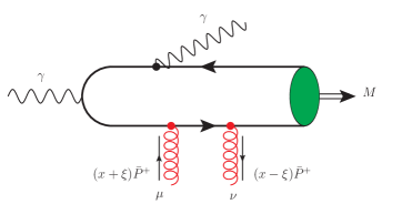
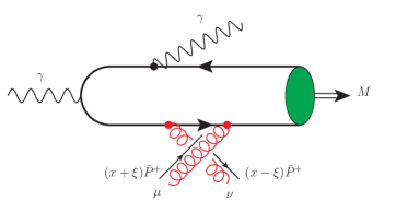
Figure 13: An illustration of the diagrams with direct and permuted $t$-channel gluons, which are related to each other by inversion of sign in front of light-cone fraction $x\leftrightarrow-x$, and permutation of the Lorentz indices $\mu\leftrightarrow\nu$.

where the first terms $\mathcal{C}\left(x,\,\xi,\,z\right)$ and $\mathcal{\tilde{C}}\left(x,\,\xi,\,z\right)$ in the right-hand sides of (48, 49) are the contributions of the six diagrams shown explicitly in the Figure   3, the second terms (with $z\to 1-z$ substitution) were obtained from charge conjugated diagrams with inverted direction of quark lines, and the last two terms (with $x\to-x$ substitution) correspond to diagrams with permuted gluons in the $t$-channel, as shown in the Figure 13. The structure of the right-hand side of (48, 49) implies that as a function of $x$, the function $c$ is even, and $\tilde{c}$ is odd. Explicitly, the components $\mathcal{C}^{(++)}\left(x,\,\xi,\,z\right)$ and $\tilde{\mathcal{C}}^{(++)}\left(x,\,\xi,\,z\right)$ are given by

$$\mathcal{C}^{(++)}\left(x,\,\xi,\,z\right)= \frac{\bar{\alpha}\mathfrak{C}_{\eta_{c}}}{4r^{2}\left(x-\xi+i0\right)\left(x+\xi-i0\right)}\times$$ (50)

$$\times \left[\frac{2\alpha z\left(2\alpha z+(\bar{\alpha}\bar{z}-\alpha)(\zeta+1)\right)-\frac{\alpha\left(4z^{3}+2z^{2}(\zeta+1)-z(4\zeta+5)+1\right)-\left(1-4z^{2}\right)\bar{z}}{r^{2}}+\frac{\left(1-4z^{2}\right)\bar{z}}{r^{4}}}{\left(\alpha\bar{z}\bar{\zeta}-\frac{4z^{2}-8z+3}{2r^{2}}-i0\right)\left(\alpha z(\zeta+1)+\frac{1-4z^{2}}{2r^{2}}-i0\right)\left((\zeta+1)+z(\alpha\,\bar{\zeta}-2)-\frac{1+4z\bar{z}}{2r^{2}}+i0\right)}\right.+$$

$$+\frac{z\left(4\alpha\bar{\alpha}z-\alpha(\zeta+1)+2\bar{z}\right)-\frac{z}{r^{2}}(\zeta+1-6\alpha z+4z)-\frac{2z^{2}}{r^{4}}}{\left(\bar{z}-\frac{1+4z\bar{z}}{4r^{2}}+i0\right)\left(\zeta+1-z(2-\alpha\bar{\zeta})-\frac{1+4z\bar{z}}{2r^{2}}+i0\right)\left(\alpha z(\zeta+1)+\frac{1-4z^{2}}{2r^{2}}-i0\right)}$$

$$+\frac{4\alpha z\left((4\alpha-2)z+\bar{\zeta}\right)-\frac{1}{r^{2}}\left(-8\bar{\alpha}z^{3}+16\alpha z^{2}+2\bar{\alpha}z-\bar{\zeta}\left(1-4z^{2}\right)\right)-\frac{2z\left(1-4z^{2}\right)}{r^{4}}}{4\left(\bar{z}-\frac{1+4z\bar{z}}{4r^{2}}+i0\right)\left(\alpha z+\frac{1-4z^{2}}{4r^{2}}-i0\right)\left(\alpha z\bar{\zeta}+\frac{1-4z^{2}}{2r^{2}}-i0\right)}$$

$$-\frac{4\alpha^{2}z\bar{z}-\frac{1}{r^{2}}\left((8\alpha-4)z^{3}-4z^{2}(3\alpha+\zeta-1)+z(2\alpha+4\zeta+1)+\zeta+1\right)-\frac{2z\left(1+4z\bar{z}\right)}{r^{4}}}{4\left(\bar{\alpha}\bar{z}+\frac{1+4z\bar{z}}{4r^{2}}-i0\right)\left(\alpha z+\frac{1-4z^{2}}{4r^{2}}-i0\right)\left(\alpha z\bar{\zeta}+\frac{1-4z^{2}}{2r^{2}}-i0\right)}$$

$$-\frac{\left(2\alpha\bar{\alpha}\bar{z}(4z-\bar{\zeta})+(2z-\bar{\zeta})^{2}\right)+\frac{4\alpha z^{3}+8z^{2}-20\alpha z^{2}+17\alpha z-2\bar{\alpha}\bar{z}\zeta-10z+2}{r^{2}}-\frac{4z^{3}-12z^{2}+7z+2}{r^{4}}}{2\left(\bar{\alpha}\bar{z}+\frac{1+4z\bar{z}}{4r^{2}}-i0\right)\left(\alpha z\bar{\zeta}+\frac{1-4z^{2}}{2r^{2}}-i0\right)\left((\alpha\bar{z}-1)\bar{\zeta}+2z-\frac{1+4z\bar{z}}{2r^{2}}+i0\right)}$$

$$+\left.\frac{-4\bar{z}\left(4\alpha\bar{\alpha}\bar{z}-\bar{\alpha}\bar{\zeta}+2z\right)+\frac{2\alpha\bar{z}\left(4z^{2}+4z-9\right)-16z^{2}\bar{z}-\zeta(1+4z\bar{z})+4\bar{z}(z+5)+1}{r^{2}}+\frac{2\bar{z}(1+4z\bar{z})}{r^{4}}}{8\left(z-\frac{1+4z\bar{z}}{4r^{2}}+i0\right)\left(\bar{\alpha}\bar{z}+\frac{1+4z\bar{z}}{4r^{2}}-i0\right)\left((\alpha\bar{z}-1)\bar{\zeta}+2z-\frac{1+4z\bar{z}}{2r^{2}}+i0\right)}\right]$$

$$\tilde{\mathcal{C}}^{(++)}\left(x,\,\xi,\,z\right)= \frac{\bar{\alpha}\mathfrak{C}_{\eta_{c}}}{4r^{2}\left(x-\xi+i0\right)\left(x+\xi-i0\right)}\times$$ (51)

$$\times \left[\frac{2\alpha z(-\alpha z\bar{\zeta}-3z\zeta+z+\zeta(\zeta+1))-\left(\frac{\alpha\left(12z^{3}+2z^{2}(\zeta-7)-3z-1\right)-4z^{3}+4z^{2}+z+1}{r^{2}}\right)-\left(\frac{-12z^{3}+12z^{2}+3z+1}{r^{4}}\right)}{\left(\alpha\bar{z}\bar{\zeta}-\frac{4z^{2}-8z+3}{2r^{2}}-i0\right)\left(\alpha z(\zeta+1)+\frac{1-4z^{2}}{2r^{2}}-i0\right)\left((\zeta+1)+z(\alpha\,\bar{\zeta}-2)-\frac{1+4z\bar{z}}{2r^{2}}+i0\right)}\right.$$

$$+\frac{z\left(4\bar{z}+2\alpha(1-2z)(\zeta+1)\right)-\frac{z}{r^{2}}\left(\alpha\left(8z^{2}-4z-2\right)+4z^{2}(\zeta-3)+16z-3\zeta+1\right)+\frac{z}{r^{4}}\left(8z^{2}-4z-2\right)}{2\left(\bar{z}-\frac{1+4z\bar{z}}{4r^{2}}+i0\right)\left(\zeta+1-z(2-\alpha\bar{\zeta})-\frac{1+4z\bar{z}}{2r^{2}}+i0\right)\left(\alpha z(\zeta+1)+\frac{1-4z^{2}}{2r^{2}}-i0\right)}$$

$$+\frac{4\alpha z((2z-1)\zeta+1)+\frac{4z\bar{z}(1+4z)-2\alpha z\left(1-4z^{2}\right)+\bar{\zeta}+2\zeta z\left(1+4z\bar{z}\right)}{r^{2}}+\frac{2z\left(1-4z^{2}\right)}{r^{4}}}{8\left(\bar{z}-\frac{1+4z\bar{z}}{4r^{2}}+i0\right)\left(\alpha z+\frac{1-4z^{2}}{4r^{2}}-i0\right)\left(\alpha z\bar{\zeta}+\frac{1-4z^{2}}{2r^{2}}-i0\right)}$$

$$+\frac{4\alpha z\bar{z}(\bar{\alpha}+\zeta)+\frac{\alpha\left(4z\bar{z}-2\right)+\bar{z}\left(1+4z\bar{z}\right)+1}{r^{2}}+\frac{2}{r^{4}}}{4\left(\bar{\alpha}\bar{z}+\frac{1+4z\bar{z}}{4r^{2}}-i0\right)\left(\alpha z+\frac{1-4z^{2}}{4r^{2}}-i0\right)\left(\alpha z\bar{\zeta}+\frac{1-4z^{2}}{2r^{2}}-i0\right)}$$

$$+\frac{\left(2\alpha^{2}\bar{z}\left(1-2z\right)\bar{\zeta}+2\alpha\bar{z}\bar{\zeta}(4z+\zeta-2)+(2z-\bar{\zeta})^{2}\right)}{2\left(\bar{\alpha}\bar{z}+\frac{1+4z\bar{z}}{4r^{2}}-i0\right)\left(\alpha z\bar{\zeta}+\frac{1-4z^{2}}{2r^{2}}-i0\right)\left((\alpha\bar{z}-1)\bar{\zeta}+2z-\frac{1+4z\bar{z}}{2r^{2}}+i0\right)}$$

$$+\frac{1}{r^{2}}\frac{-\alpha r^{2}\left(12z^{3}-16z^{2}-z+4-2\zeta\bar{z}(1-2z)\right)-2r^{2}\bar{z}\left(4z^{2}+\zeta-2\right)+\left(2-3z\right)\left(1+4z\bar{z}\right)}{2\left(\bar{\alpha}\bar{z}+\frac{1+4z\bar{z}}{4r^{2}}-i0\right)\left(\alpha z\bar{\zeta}+\frac{1-4z^{2}}{2r^{2}}-i0\right)\left((\alpha\bar{z}-1)\bar{\zeta}+2z-\frac{1+4z\bar{z}}{2r^{2}}+i0\right)}$$

$$+\left.\frac{4\bar{z}(2\alpha z(\zeta+1)-\bar{\alpha}\bar{\zeta}-2z)+\frac{-2\alpha\bar{z}\left(1+4z\bar{z}\right)+\bar{\zeta}(8z^{3}-20z^{2}+10z+1)-16z\bar{z}}{r^{2}}+\frac{2\bar{z}\left(1+4z\bar{z}\right)}{r^{4}}}{8\left(z-\frac{1+4z\bar{z}}{4r^{2}}+i0\right)\left(\bar{\alpha}\bar{z}+\frac{1+4z\bar{z}}{4r^{2}}-i0\right)\left((\alpha\bar{z}-1)\bar{\zeta}+2z-\frac{1+4z\bar{z}}{2r^{2}}+i0\right)}\right]$$

where $r=M_{\gamma\eta_{c}}/M_{\eta_{c}}\approx\sqrt{2\xi s}/2m_{c}$, $\alpha\equiv\alpha_{\eta_{c}}$, $\bar{\alpha}\equiv 1-\alpha_{\eta_{c}}$, $\bar{z}\equiv 1-z$, $\zeta=x/\xi$, the contour deformation prescription was derived from the conventional $m_{c}^{2}\to m_{c}^{2}-i0$ prescription in denominators of Feynman propagators, and the constant $\mathfrak{C}_{\eta_{c}}$ was defined earlier in (27). The expressions for the helicity flip components $\mathcal{C}^{(+-)},\,\mathcal{\tilde{C}}^{(+-)}$ have a similar structure, though have additional $\sim\mathcal{O}\left(1/r^{2}\right)$ suppression due to cancellation of the leading order term in the numerator. In the limit $z_{1}=z_{2}=1/2$ these expressions reduce to (23-26) from the main text.

In our expressions (50,51) we ordered the terms by their behavior in the limit $r\to\infty$. This limit corresponds to the high energy limit ($s\to\infty$) at fixed heavy quarkonium mass $M_{\eta_{c}}$, as well as to the limit of negligibly small meson mass at fixed invariant mass $M_{\gamma\eta_{c}}={\rm const}$ (so that $r=M_{\gamma\eta_{c}}/M_{\eta_{c}}\to\infty$). We may check that in this limit for $C_{\gamma\eta_{c}}^{(++)}$ we may recover the Eq. (A3) from  Nabeebaccus:2023 ,

$$\lim_{r\to\infty}C_{\gamma\eta_{c}}^{(++)}\left(x,\,\xi,\,z\right)\sim\frac{\left(1-\alpha/2\right)\left(x^{2}-\xi^{2}\right)}{\left(x+\xi-i0\right)^{2}\left(x-\xi+i0\right)^{2}}\times$$ (52)

$$\times\frac{(1-\alpha)\left(\left(x^{2}-\xi^{2}\right)^{2}(1-2z\bar{z})+8\xi^{2}x^{2}z\bar{z}\right)+\left(x^{4}-\xi^{4}\right)z\bar{z}\left(1+\bar{\alpha}^{2}\right)}{\left(\bar{z}(x+\xi)-\bar{\alpha}z(x-\xi)-i0\right)\left(z(x-\xi)+\bar{\alpha}\bar{z}(x+\xi)-i0\right)\left(\bar{z}(x-\xi)+\bar{\alpha}z(x+\xi)-i0\right)\left(z(x+\xi)-\bar{\alpha}\bar{z}(x-\xi)-i0\right)}.$$

where we switched to conventional notations in terms of $x,\,\xi$. As was explained in Nabeebaccus:2023 , the coefficient function  (52) after convolution with gluon GPDs and meson LCDAs might lead to the singular amplitudes when several singularities overlap and start pinching the contour. Typically, this occurs when one of the $t$-channel gluons is soft ($x=\pm\xi$) and interacts with a soft quark from the final meson ($z$ or $\bar{z}=0$). From the structure of the denominators in (50,51) we can see that in case of the massive theory with finite $r\not=\infty$ this no longer happens, since $\sim\mathcal{O}\left(1/r^{2}\right)$ corrections in denominators shift the position of the poles, thus avoiding overlaps. For some terms the constants in front of $\sim\mathcal{O}\left(1/r^{2}\right)$ terms vanish in the point $z=1/2$, thus leading to an overlapping poles at $x=\pm\xi$ . We checked explicitly that in all such points these singularities are located on the same side of the integration contour and do not pinch it. For this reason, the integration near such second-order pole does not lead to physical singularity and may be performed using the conventional rule (30).

In order to estimate numerically the role of the finite width of the $\eta_{c}$ wave function, we calculated the cross-section using convolution with normalized to unity light-cone DA from  Dosch:1996ss . We found that this changes the cross-sections not more than 20 per cent compared to NRQCD approach (37,38), on par with expected contributions due to higher order $\mathcal{O}\left(\alpha_{s}(m_{c})\right)$ corrections.

References

- (1) M. Diehl, T. Feldmann, R. Jakob and P. Kroll, Nucl. Phys. B 596, 33 (2001) [Erratum-ibid. B 605, 647 (2001)] [arXiv:hep-ph/0009255].
- (2) K. Goeke, M. V. Polyakov and M. Vanderhaeghen, Prog. Part. Nucl. Phys. 47, 401 (2001) [arXiv:hep-ph/0106012].
- (3) M. Diehl, Phys. Rept. 388, 41 (2003) [arXiv:hep-ph/0307382].
- (4) M. Guidal, H. Moutarde and M. Vanderhaeghen, “Generalized Parton Distributions in the valence region from Deeply Virtual Compton Scattering,” Rept. Prog. Phys. 76 (2013), 066202 [arXiv:1303.6600 [hep-ph]].
- (5) D. Boer, M. Diehl, R. Milner, R. Venugopalan, W. Vogelsang, D. Kaplan, H. Montgomery, S. Vigdor, A. Accardi and E. C. Aschenauer, et al. “Gluons and the quark sea at high energies: Distributions, polarization, tomography,” [arXiv:1108.1713 [nucl-th]].
- (6) H. Dutrieux, C. Lorcé, H. Moutarde, P. Sznajder, A. Trawinski and J. Wagner, “Phenomenological assessment of proton mechanical properties from deeply virtual Compton scattering,” Eur. Phys. J. C 81, no.4, 300 (2021) [arXiv:2101.03855 [hep-ph]].
- (7) V. Burkert, L. Elouadrhiri, A. Afanasev, J. Arrington, M. Contalbrigo, W. Cosyn, A. Deshpande, D. Glazier, X. Ji and S. Liuti, et al. “Precision Studies of QCD in the Low Energy Domain of the EIC,” [arXiv:2211.15746 [nucl-ex]].
- (8) R. Abdul Khalek et al. “Science Requirements and Detector Concepts for the Electron-Ion Collider: EIC Yellow Report,” [arXiv:2103.05419 [physics.ins-det]].
- (9) A. Accardi et al., Eur. Phys. J. A 52, no. 9, 268 (2016) [arXiv:1212.1701 [nucl-ex]].
- (10) K. Kumericki, S. Liuti and H. Moutarde, “GPD phenomenology and DVCS fitting: Entering the high-precision era,” Eur. Phys. J. A 52 (2016) no.6, 157 [arXiv:1602.02763 [hep-ph]].
- (11) V. Bertone, H.Dutrieux, C.Mezrag, H.Moutarde and P.Sznajder,“Deconvolution problem of deeply virtual Compton scattering,” Phys. Rev. D 103, no.11, 114019 (2021) [arXiv:2104.03836 [hep-ph]].
- (12) E.Moffat, A.Freese, I. Cloët, T. Donohoe, L. Gamberg, W. Melnitchouk, A. Metz, A. Prokudin and N. Sato, “Shedding light on shadow generalized parton distributions,” Phys. Rev. D 108, no.3, 036027 (2023) [arXiv:2303.12006 [hep-ph]].
- (13) Y. Guo, X. Ji, M. G. Santiago, K. Shiells and J. Yang, “Generalized parton distributions through universal moment parameterization: non-zero skewness case,” JHEP 05, 150 (2023) [arXiv:2302.07279 [hep-ph]].
- (14) G. Duplančić, S. Nabeebaccus, K. Passek-Kumerički, B. Pire, L. Szymanowski and S. Wallon, “Accessing chiral-even quark generalised parton distributions in the exclusive photoproduction of a pair with large invariant mass in both fixed-target and collider experiments,” [arXiv:2212.00655 [hep-ph]].
- (15) G. Duplančić, K. Passek-Passek-Kumerički, B. Pire, L. Szymanowski and S. Wallon, JHEP 11 (2018) 179 [arXiv:1809.08104 [hep-ph]].
- (16) R. Boussarie, B. Pire, L. Szymanowski and S. Wallon, JHEP 02 (2017) 054 [erratum: JHEP 10 (2018), 029] [arXiv:1609.03830 [hep-ph]].
- (17) W. Cosyn and B. Pire, Phys. Rev. D 103 (2021) 114002 [arXiv:2103.01411 [hep-ph]].
- (18) A. Pedrak, B. Pire, L. Szymanowski and J. Wagner, Phys. Rev. D 101 (2020) 114027 [arXiv:2003.03263 [hep-ph]].
- (19) B. Pire, L. Szymanowski and S. Wallon, Phys. Rev. D 101 (2020) 074005 [arXiv:1912.10353 [hep-ph]].
- (20) A. Pedrak, B. Pire, L. Szymanowski and J. Wagner, Phys. Rev. D 96 (2017) 074008 [arXiv:1708.01043 [hep-ph]].
- (21) M. El Beiyad, B. Pire, M. Segond, L. Szymanowski and S. Wallon, Phys. Lett. B 688 (2010) 154 [arXiv:1001.4491 [hep-ph]].
- (22) D.Y. Ivanov, B. Pire, L. Szymanowski and O.V. Teryaev, Phys. Lett. B 550 (2002) 65 [arXiv:hep-ph/0209300].
- (23) G. Duplančić, S. Nabeebaccus, K. Passek-Kumerički, B. Pire, L. Szymanowski and S. Wallon, “Accessing GPDs through the exclusive photoproduction of a photon-meson pair with a large invariant mass,” [arXiv:2212.01034 [hep-ph]].
- (24) J. W. Qiu and Z. Yu, “Extracting transition generalized parton distributions from hard exclusive pion-nucleon scattering,” Phys. Rev. D 109, no.7, 074023 (2024) [arXiv:2401.13207 [hep-ph]].
- (25) J. W. Qiu and Z. Yu, “Extraction of the Parton Momentum-Fraction Dependence of Generalized Parton Distributions from Exclusive Photoproduction,” Phys. Rev. Lett. 131, no.16, 161902 (2023) [arXiv:2305.15397 [hep-ph]].
- (26) K. Deja, V. Martinez-Fernandez, B. Pire, P. Sznajder and J. Wagner, “Phenomenology of double deeply virtual Compton scattering in the era of new experiments,” Phys. Rev. D 107, no.9, 094035 (2023) [arXiv:2303.13668 [hep-ph]].
- (27) M. Siddikov and I. Schmidt, “Exclusive production of quarkonia pairs in collinear factorization framework,” Phys. Rev. D 107 (2023) no.3, 034037 [arXiv:2212.14019 [hep-ph]].
- (28) M. Siddikov and I. Schmidt, “Exclusive photoproduction of D-meson pairs with large invariant mass,” Phys. Rev. D 108 (2023) no.9, 096031 [arXiv:2309.09748 [hep-ph]].
- (29) J.-W. Qiu and Z. Yu, “Exclusive production of a pair of high transverse momentum photons in pion-nucleon collisions for extracting generalized parton distributions”, [arXiv:2205.07846 [hep-ph]].
- (30) J.-W. Qiu and Z. Yu, “Single diffractive hard exclusive processes for the study of generalized parton distributions”, [arXiv:2210.07995 [hep-ph]].
- (31) G.Duplan, S.Nabeebaccus, K.Passek-Kumericki, B.Pire, J. Schönleber, L.Szymanowski and S.Wallon, [arXiv:2401.17656 [hep-ph]].
- (32) S.Nabeebaccus, J. Schönleber, L. Szymanowski and S.Wallon, [arXiv:2311.09146 [hep-ph]].
- (33) J. G. Korner and G. Thompson, Phys. Lett. B 264, 185 (1991).
- (34) M. Neubert, “Heavy quark symmetry,” Phys. Rept. 245 (1994), 259-396 [arXiv:hep-ph/9306320 [hep-ph]].
- (35) G. T. Bodwin, E. Braaten and G. P. Lepage, Phys. Rev. D 51, 1125 (1995) Erratum: [Phys. Rev. D 55, 5853 (1997)] [hep-ph/9407339].
- (36) F. Maltoni, M. L. Mangano and A. Petrelli, Nucl. Phys. B 519, 361 (1998) [hep-ph/9708349].
- (37) N. Brambilla, E. Mereghetti and A. Vairo, Phys. Rev. D 79, 074002 (2009) Erratum: [Phys. Rev. D 83, 079904 (2011)] [arXiv:0810.2259 [hep-ph]].
- (38) Y. Feng, J. P. Lansberg and J. X. Wang, Eur. Phys. J. C 75, no. 7, 313 (2015) [arXiv:1504.00317 [hep-ph]].
- (39) N. Brambilla et al.; Eur. Phys. J. C71, 1534 (2011).
- (40) P. L. Cho and A. K. Leibovich, Phys. Rev. D 53, 6203 (1996) [hep-ph/9511315].
- (41) P. L. Cho and A. K. Leibovich, Phys. Rev. D 53, 150 (1996) [hep-ph/9505329].
- (42) S. P. Baranov, Phys. Rev. D 66, 114003 (2002).
- (43) S. P. Baranov and A. Szczurek, Phys. Rev. D 77, 054016 (2008) [arXiv:0710.1792 [hep-ph]].
- (44) S. P. Baranov, A. V. Lipatov and N. P. Zotov, Phys. Rev. D 85, 014034 (2012) [arXiv:1108.2856 [hep-ph]].
- (45) S. P. Baranov and A. V. Lipatov, Phys. Rev. D 96, no. 3, 034019 (2017) [arXiv:1611.10141 [hep-ph]].
- (46) S.P. Baranov, A.V. Lipatov, N.P. Zotov; Eur. Phys. J. C75, 455 (2015).
- (47) D.Yu. Ivanov, A. Schafer, L. Szymanowski and G. Krasnikov, Eur. Phys. J. C 34 (2004) 297, [arXiv:hep-ph/0401131].
- (48) M. Vanttinen and L. Mankiewicz, Phys. Lett. B 440 (1998) 157, [arXiv:hep-ph/9807287].
- (49) J. Koempel, P. Kroll, A. Metz and J. Zhou, Phys. Rev. D 85 (2012) 051502 [arXiv:1112.1334 [hep-ph]].
- (50) Z.L. Cui, M.C. Hu and J.P. Ma, Eur. Phys. J C 79 (2019), 812 [aXiv:1804.05293 [hep-ph]].
- (51) L.A.Harland-Lang, V.A.Khoze, A.D.Martin and M.G.Ryskin,“Searching for the Odderon in Ultraperipheral Proton–Ion Collisions at the LHC,” Phys. Rev. D 99, no.3, 034011 (2019), [arXiv:1811.12705 [hep-ph]].
- (52) A. Accardi, P. Achenbach, D. Adhikari, A. Afanasev, C. S. Akondi, N. Akopov, M. Albaladejo, H. Albataineh, M. Albrecht and B. Almeida-Zamora, et al. “Strong Interaction Physics at the Luminosity Frontier with 22 GeV Electrons at Jefferson Lab,” [arXiv:2306.09360 [nucl-ex]].
- (53) A. Schäfer, L. Mankiewicz, and O. Nachtmann, Diffractive eta(c), eta-prime, J/psi and psi-prime production in electronproton collisions at HERA energies, in Proceedings of “Physics at HERA,” edited by W. Buchmüller and G. Ingelman (DESY, Hamburg, Germany, 1992).
- (54) J. Czyzewski, J. Kwiecinski, L.Motyka, and M. Sadzikowski, Phys. Lett. B 398, 400 (1997); 411, 402 (1997).
- (55) R. Engel, D. Y. Ivanov, R. Kirschner, and L. Szymanowski, Eur. Phys. J. C 4, 93 (1998).
- (56) A. Dumitru, T. Stebel, Phys. Rev. D 99, 094038 (2019).
- (57) C. F. von Weizsacker, “Radiation emitted in collisions of very fast electrons,” Z. Phys. 88, 612 (1934).
- (58) [85] E. J. Williams, “Correlation of certain collision problems with radiation theory,” Kong. Dan. Vid. Sel. Mat. Fys. Med. 13N4, 1 (1935).
- (59) V. M. Budnev, I. F. Ginzburg, G. V. Meledin and V. G. Serbo, “The Two photon particle production mechanism. Physical problems. Applications. Equivalent photon approximation,” Phys. Rept. 15 (1975), 181-281.
- (60) A. V. Belitsky, D. Mueller and A. Kirchner, Nucl. Phys. B 629, 323 (2002) [arXiv:hep-ph/0112108].
- (61) A. V. Belitsky and A. V. Radyushkin, Phys. Rept. 418, 1 (2005) [arXiv:hep-ph/0504030].
- (62) E. Braaten and J. Lee, “Exclusive Double Charmonium Production from Annihilation into a Virtual Photon,” Phys. Rev. D 67 (2003), 054007 [erratum: Phys. Rev. D 72 (2005), 099901] [arXiv:hep-ph/0211085 [hep-ph]].
- (63) S. V. Goloskokov and P. Kroll, Eur. Phys. J. C 50, 829 (2007) [hep-ph/0611290].
- (64) S. V. Goloskokov and P. Kroll, Eur. Phys. J. C 53, 367 (2008) [arXiv:0708.3569 [hep-ph]].
- (65) S. V. Goloskokov and P. Kroll, Eur. Phys. J. C 59 (2009) 809 [arXiv:0809.4126 [hep-ph]].
- (66) S. V. Goloskokov and P. Kroll, Eur. Phys. J. C 65, 137 (2010) [arXiv:0906.0460 [hep-ph]].
- (67) S. V. Goloskokov and P. Kroll, Eur. Phys. J. A 47, 112 (2011) [arXiv:1106.4897 [hep-ph]].
- (68) S. Navas et al. [Particle Data Group], Phys. Rev. D 110, 030001 (2024).
- (69) M. Ablikim et al. [BESIII], “Measurements of the branching fractions of , ,, and ,” Phys. Rev. D 100 (2019) no.1, 012003 [arXiv:1903.05375 [hep-ex]].
- (70) J. Bartels, Nucl. Phys. B175, 365 (1980); T. Jaroszewicz, Acta Phys. Polon. B 11, 965 (1980); J. Kwiecinski and M. Praszalowicz, Phys. Lett. 94B, 413 (1980).
- (71) L. Lukaszuk and B. Nicolescu, Lett. Nuovo Cim. 8, 405 (1973); D. Joynson, E. Leader, B. Nicolescu, and C. Lopez, Nuovo Cimento A 30, 345 (1975).
- (72) C. Ewerz, arXiv:hep-ph/0306137.
- (73) S. Benic, D. Horvatic, A. Kaushik, and E. A. Vivoda, “Exclusive production from small-x evolved Odderon at a electron-ion collider,” Phys.Rev. D 108 (2023) 7, 074005. [arXiv:2306.10626 [hep-ph]].
- (74) G. Antchev et al. (TOTEM Collaboration), arXiv:1812.08610.
- (75) V. M. Abazov et al. (D0 Collaboration), Phys. Rev. D 86, 012009 (2012).
- (76) G. P. Lepage and S. J. Brodsky, “Exclusive processes in perturbative quantum chromodynamics”, Phys. Rev. D 22 (1980) 2157.
- (77) S. J. Brodsky, H. C. Pauli and S. S. Pinsky, “Quantum chromodynamics and other field theories on the light cone,” Phys. Rept. 301 (1998), 299-486 [arXiv:hep-ph/9705477 [hep-ph]].
- (78) M. Diehl, T. Gousset and B. Pire, “Polarization in deeply virtual meson production,” [arXiv:hep-ph/9909445 [hep-ph]].
- (79) X. D. Ji, J. Phys. G 24, 1181 (1998) [arXiv:hep-ph/9807358].
- (80) J. P. Ma and Z. G. Si, “NRQCD Factorization for Twist-2 Light-Cone Wave-Functions of Charmonia,” Phys. Lett. B 647 (2007), 419-426 [arXiv:hep-ph/0608221 [hep-ph]].
- (81) X. P. Wang and D. Yang, “The leading twist light-cone distribution amplitudes for the S-wave and P-wave quarkonia and their applications in single quarkonium exclusive productions,” JHEP 06 (2014), 121 [arXiv:1401.0122 [hep-ph]].
- (82) W. Wang, J. Xu, D. Yang and S. Zhao, “Relativistic corrections to light-cone distribution amplitudes of S-wave mesons and heavy quarkonia,” JHEP 12 (2017), 012 [arXiv:1706.06241 [hep-ph]].
- (83) V.M. Braun and I.B. Filyanov, Z. Phys. C48 (1990) 239,
- (84) P. Ball, JHEP 01 (1999) 010.
- (85) P. Ball and V.M. Braun, Phys.Rev. D54 (1996) 2182.
- (86) P. Ball, V. M. Braun, Y. Koike and K. Tanaka, Nucl.Phys. B529 (1998) 323.
- (87) P. Ball and V.M. Braun, Nucl.Phys. B543 (1999) 201.
- (88) H. G. Dosch, T. Gousset, G. Kulzinger and H. J. Pirner, “Vector meson leptoproduction and nonperturbative gluon fluctuations in QCD,” Phys. Rev. D 55 (1997), 2602-2615 [arXiv:hep-ph/9608203 [hep-ph]].