Geometry of homogeneous polynomials in
Abstract.
This work is a thorough and detailed study on the geometry of the unit sphere of certain Banach spaces of homogeneous polynomials in . Specifically, we provide a complete description of the unit spheres, identify the extreme points of the unit balls, derive explicit formulas for the corresponding polynomial norms, and describe the techniques required to tackle these questions.
To enhance the comprehensiveness of this work, we complement the results and their proofs with suitable diagrams and figures. The new results presented here settle some open questions posed in the past. For the sake of completeness of this work, we briefly discuss previous known results and provide directions of research and applications of our results.
Key words and phrases:
Convexity, Extreme Points, Polynomial Norms, Trinomials2020 Mathematics Subject Classification:
52A21, 46B04Corresponding author: Mingu Jung. Email: jmingoo@kias.re.kr
1. Introduction
The study of the unit ball of a polynomial space has motivated a significant volume of publications. However, this problem has much earlier roots. As early as 1966, Konheim and Rivlin [KoRi] provided a characteristic property of the extreme points of the unit ball of the space , which consists of polynomials on the real line of degree at most , endowed with the norm
The search for characterizations of the extreme points of the unit ball of a polynomial space intensified since the late 1990’s. The references [GaGrMa, Di3, AK, BMRS, CK1, CK2, CK3, GMSS, ChKiKi, G1, G2, G3, G4, G5, G6, G7, MN1, MN2, MN3, MPSW, MRS, MS, N, RyTu, MR4740398] are just a selection of contributions to the study of the geometry of a number of polynomial spaces of low dimension. The interested reader can find a monograph on this topic in [FGMMRS].
Interestingly, polynomial norms are frequently non-absolute. Recall that a norm on a linear subspace of (here, is any non-empty set) is absolute whenever it is complete and satisfies the following conditions:
-
(a)
Given with for every , if , then with .
-
(b)
For every , the function given by for , belongs to with .
One property which can be deduced from the definition is the following: given with for every , if , then with . The -norms together with many other classical norms are clearly absolute in . Hence polynomial norms can be viewed as a source of natural examples of non-absolute norms.
Perhaps one of the most relevant motivations to study polynomial spaces, and more specifically the extreme points of their unit balls, rests on the fact that an elementary application of the Krein-Milman theorem allows us to obtain optimal constants in a number of polynomial inequalities of interest. For instance, in [AMRS, AJMS, MSS, JMPS, MSanSeo1, MSanSeo2, V, AAMarkov, ENG, KoRi] one can find several applications that obtain optimal Bernstein and Markov type estimates using a combination of geometric results and the so-called Krein-Milman approach. Similarly, several polynomial Bohnenblust-Hille type inequalities (see, e.g., [DGMPbook, MR3250297, MR4740398]) can be derived (see, for instance, [JMMS, DMPS, MPS]). The same techniques can be applied to obtain sharp estimates of polarization constants and unconditional constants (see [MRS, G7]) and many other polynomial inequalities of interest (see, for instance, [AEMRS, AJMS2]).
We now provide a precise definition of the polynomial space that will be examined in this paper. Consider the space consisting of the homogeneous trinomials on the plane where and are such that . That space, endowed with the norm
will be denoted by . The aim of this paper is to explore the geometry of the unit ball of , extending and generalizing the results established by Choi, Kim, and Ki in 1998 [ChKiKi], Aron and Klimek in 2001 [AK], and Muñoz and Seoane in 2008 [MS]. Furthermore, we complete the investigation of that was initiated in [JMR2021] and [GMS2023].
In particular, we will provide a complete description of the unit sphere in and characterize the extreme points of the unit ball in . The solutions to these two questions depend significantly on whether and are even or odd. A thorough analysis reveals that the problem must be examined in the following three main cases:
Cases A and B have been previously studied in [JMR2021] and [GMS2023], respectively. For the sake of completeness, we will present the known results for each case in the following.
1.1. Case A: is odd
For Case A, the detailed study of the geometry of the unit sphere of needs to be divided into two different subcases, depending on whether or (since is not possible in this case). Although the two subcases within Case A are similar, let us briefly describe below what the geometry of the unit balls “looks like.”
As mentioned earlier, the study of the geometry of depends strongly on whether and are even or odd and each of the four possible choices of the parity of and requires a specific treatment (see [MS]). As a related space to , consider the space consisting of the trinomials in the real line of the form endowed with the norm
For simplicity, we will frequently use the representation of the polynomials or as the triple , that is,
-
, and
-
.
The norms and are tightly related; in fact, using the fact that the elements of attain their norm on the set by homogeneity and symmetry, it is not difficult to see that
| (1.1) |
for every . The previous identity reveals that
| (1.2) |
for every . The identity (1.2) allows us to simplify the study of the geometry of , at least when is odd. The case where both and are odd can be reduced to the case where is odd and is even by swapping and on the one hand, and and on the other. Thus, in order to describe the Case A, we shall focus our attention on the case odd and even. First, let us present the following auxiliary result, followed by the explicit formulas for the norm .
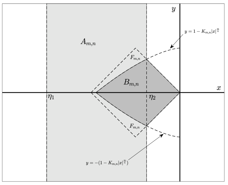
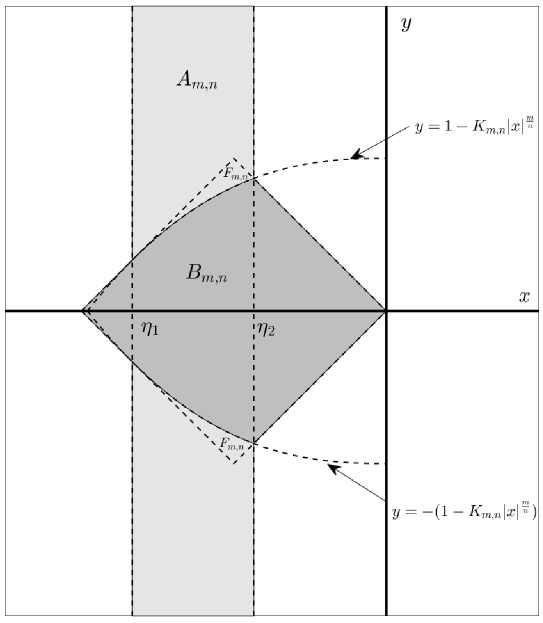
Proposition 1.1 ([MS, Lemma 2.1]).
If are such that then the equation
has only three roots, one at , another one at a point and a third one at a point . In addition to that we have
| (1.3) |
if and only if or .
Remark 1.2.
Proposition 1.3 ([JMR2021, Theorem 3.4]).
Once the formulas for the norm are provided, a different matter is to obtain the set of extreme points for the unit ball. In this Case A, the description of extreme points of are given in [JMR2021], namely:
Proposition 1.4 ([JMR2021, Theorem 3.6]).
Let be such that , is odd and is even and suppose that
We have:
-
If , then
-
If , then
These extreme points are spotted in Figures 3 and 4 (which are represented for some choices of and ).
1.2. Case B: and are both even
Regarding Case B, where both and are even, the study of the norm and geometry of the unit sphere is highly technical and complex. In this case, we need to consider three different situations: , , and . The outcomes differ quite a bit depending on each situation. To make this paper self-contained, we will present these results as well, which can be found in [GMS2023].
First, regarding the explicit formula of in this case, we have the following:
Proposition 1.5 ([GMS2023, Theroem 2.6]).
Of course, the description of the extreme points of the corresponding unit sphere is also hard to tackle; however, this was successfully achieved in [GMS2023].
Proposition 1.6 ([GMS2023, Theorem 4.2]).
Let be even numbers with . Also, as earlier, we let , and The set of extreme points is given by
-
(1)
If then
-
(2)
If then
-
(3)
If then
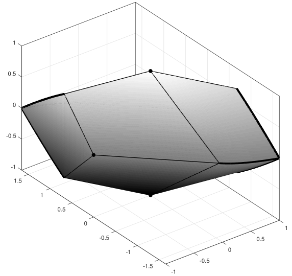
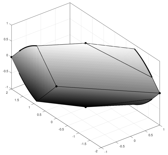
Some sketches of the unit spheres together with the corresponding sets of extreme points are shown in Figures 7 and 8.
Certainly, as the reader can see, Case B is way more complex than Case A, at least at first sight. In fact, delving into the details and technicalities of the constructions from [JMR2021] or [GMS2023] (see also the recent monograph [FGMMRS]), one realizes that these types of problems are far from easy to tackle.
1.3. Outline of our paper
So far, we have briefly discussed the formulas for and the complete descriptions of the extreme points of in Case A and Case B.
One of the most challenging aspects of solving Case C is that many of the equations that naturally arise in the computation are implicit, unlike the explicit equations encountered in Case A or Case B. One way to address this difficulty is by implementing an appropriate change of variables, which requires considering two different coordinate systems simultaneously. Despite these difficulties, the rest of the paper will be devoted to solving Case C. From now on, unless otherwise specified, and will be positive integers such that , with being even and being odd. Solving this final case will complete the general analysis, covering all possibilities for and .
The outline of the rest of this paper is as follows: Section 2 is devoted to obtain an explicit formula for for all positive integers with even and odd. The formula obtained in Section 2 will be used in Section 3 to calculate the projection of over the plane together with a parametrization of . Thanks to the results in Sections 2 and 3, we will be able to complete this thorough study by providing the extreme points of in Section 4; thus resolving Case C. Additionally, the sphere will be sketched for several choices of and .
The following notations will be useful to understand the rest of the paper. If is a convex body, will denote the set of extreme points of . Also, will denote the linear projection given by , for every . The plots of and the projection , together with some other figures appearing in this paper were generated using MATLAB. All graphs presented here are scaled.
2. A formula for with even and odd
Given with and , recall from (1.1) and (1.2) that
and
The second identity allows us to simplify some of the forthcoming proofs in the sense that it will be enough to consider the case where .
In [MS], the authors derived a formula to calculate and , which we will state for completeness in the following result:
Theorem 2.1 (Muñoz and Seoane, [MS, Theorem 4.1]).
For every with even, odd and , let us define as the set of triples such that
Then we have
| (2.1) |
In the first main result of this paper, we will derive a formula to calculate for the case where is even, is odd, and . We will introduce necessary definitions and auxiliary results.
Lemma 2.2.
Let and be positive integers such that is even, is odd and . Consider the regions and from Theorem 2.1. Define
Then
-
(1)
and
-
(2)
,
where
and .
Proof.
Let us prove first . Using the definition of , we have that if and only if
and
Let for . Since is even, we just need to investigate in , where is given by . It is elementary to show that vanishes only at and that . Hence has its absolute miminum at and therefore is strictly decreasing in . Consequently attains it maximun at and so for all . Now observe that if and only if . This allows us to focus on the pairs with non negative . Let us take . Assume first that . Then is equivalent to
On the other hand, the inequality is equivalent to
Then multiplying the previous inequality by (which is positive) we arrive at the equivalent condition
or
If it is straightforward that if and only if . Also . Then we have shown that, for with , if and only if
and
finishing the proof of .
Now we prove . From the definition of (see Theorem 2.1), is equivalent to
| (2.2) |
and
| (2.3) |
Clearly, if and only if . In the rest of the proof we may assume then that . Assume first that . Writing (2.2) and (2.3) in terms of we obtain
and
or equivalently
and
| (2.4) |
If for all with , then attains it absolute maximum at . Indeed, we just need to notice that is even and that for all . Then for all with . In particular, from (2.4) it follows that , and since , then Consequently, (2.4) would be equivalent to
If then and , proving that with is equivalent to
and
This concludes the proof of . ∎
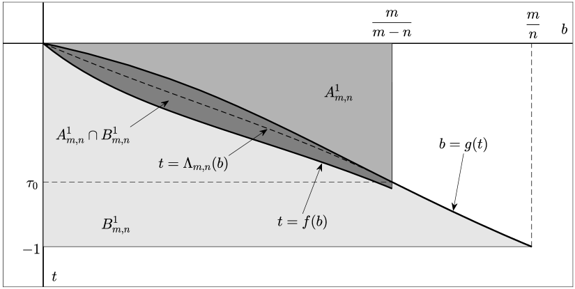
In the following, on many occasions it will be useful to replace the variable by the variable with . Doing so it is straightforward that (respectively ) if and only if (respectively ) where and with , and
It is a good moment to take a look at the representation of and in Figure 10.
Lemma 2.3.
Let and be positive integers such that is even, is odd and . If , the equation
| (2.5) |
defines an strictly decreasing function defined for such that . We define .
Proof.
If exists then it is straightforward that . Now, differentiating (2.5) with respect to we arrive at
Hence, if exists, it must be a solution to the initial value problem
| (2.6) |
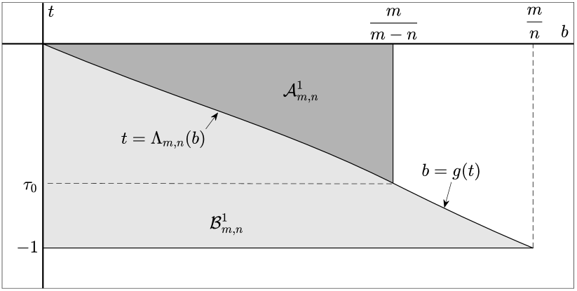
Now consider the open subset of given by
The set has been represented in Figure 9. Observe that . Then, since and are both continuous in , the initial value problem (2.6) has a unique solution that can be extended to .
On the other hand, dividing (2.5) by (assuming ),
Differentiating again with respect to ,
which is clearly negative for every plausible value of and . Hence is strictly decreasing and its domain contains and therefore too. ∎
Remark 2.4.
The value of for every plausible choice of and is the unique solution between and of the equation
| (2.7) |
The equation (2.7) cannot generally be solved explicitly. However, using specialized software can be approximated with precision. We provide below a table with some approximations to obtained with Mathematica:
For and (or in any case) it can be seen that is exactly equal to
To give the reader an idea of how complex these calculations can get, for low values of and , is a real root of a polynomial. For instance, if and , is the only real root of the degree polynomial given by
Theorem 2.5.
Proof.
It is elementary to prove that
for all . Also,
| (2.9) |
For the rest of the proof we will assume that . In particular we have
and therefore it will be enough to obtain a formula to calculate for all with .
According to (1.1) we have
Now using (2.1) we obtain
Since and we can assume that . From Lemma 2.2 we have:
-
•
is equivalent to .
-
•
is equivalent to .
As a matter of fact, since in fact we have
-
•
is equivalent to .
-
•
is equivalent to .
Therefore, if we have that
and
whenever . To finish the proof we just need to compare and within .
It is left to the reader to check that the inequality
can be written using the variables and as
| (2.10) |
Now, let and be, respectively, the right and the left hand side of (2.10). Notice that
for every and
for all with . The equality
is equivalent to
which is the identity (2.5) studied in Lemma 2.3. Hence and coincide only along the curve . Interestingly, and meet at the point . Indeed, from Lemma 2.3, keeping in mind that , and making
which entails that , we have the identity
After some straightforward calculations we arrive at
| (2.11) |
Next, let us see that
Indeed, using equation (2.11), we have
Also, let us notice that equation (2.11) has only one solution in the interval . Indeed, using a convexity argument, it is clear that the functions and meet, at most, twice. Since makes and we know that there is one solution belonging to , the above in unique.
We conclude that if and is below the curve or in the curve, or equivalently in . On the contrary in the rest of or along the curve , that is, in . Then
We arrive at the desired result by combining the previous formula with
∎
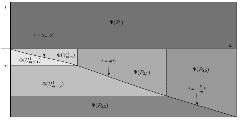
3. A parametrization of the unit sphere
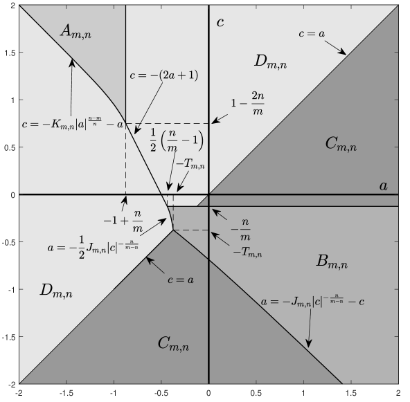
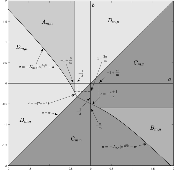
In order to obtain a parametrization of it will be necessary to know the projection of over a plane. The most convenient plane is (also called the plane) since the unit ball is symmetric with respect to that plane. The latter is justified with the obvious equation whenever is even and odd.
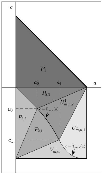
In the main result of this section some notations and definitions will be needed. First we consider two curves that will play an important role, namely and . The first curve is defined implicitly using the following lemma.
Lemma 3.1.
Let be positive integers such that , is even and is odd. Define the numbers and and consider the equation
| (3.1) |
Then in (3.1) can be expressed as a function of with , namely , where the curve meets the parallel lines and at the points and respectively (see Figure 12). Moreover, is strictly decreasing and for . It turns out that
whereas and cannot generally be obtained explicitly.
Proof.
One can check easily that with and is a solution to (3.1) and that the line passes though . Notice that for each fixed , the function
is a strictly decreasing function. It is clear that . Observe also that
is strictly decreasing; so
where the last equality holds since the intersection point satisfies the equation (3.1). By Intermediate Value Theorem, this shows that there exists a unique such that , i.e., satisfies the equation (3.1).
Next, differentiating (3.1) with respect to we obtain
for all . Then if exists, it must be the solution of the initial value problem for a given point ,
| (3.2) |
Since and are both continuous in , the Picard-Lindelöf theorem shows that the initial value problem (3.2) has a unique solution (which is ) around some interval containing . By uniqueness, this local solution coincides with the one given from Intermediate Value Theorem locally. Since is given arbitrarily, we conclude that exists and is well-defined for all . Also is strictly decreasing and the curve meets the straight line at the point with and . ∎
Also, we will consider the curve with where
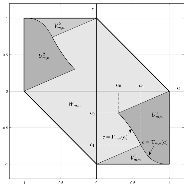
Interestingly, the curves , and the straight line meet at the point (see Figure 12). Also, for every pair of positive integers with , even and odd, we will use the sets , , , , , , and defined as
where , and
See Figure 12 for a representation of , , and .
Theorem 3.2.
Let be such that with even and odd. Then
Proof.
Since is symmetric with respect to the plane , it is clear that is the intersection of and the plane , that is,
In other words, if and only if . Using (2.9) it follows straightforwardly that
as desired. ∎
Next we are going to parametrize the unit sphere . Recall that if then is nothing but the space , whose unit ball was already studied by Choi and Kim in [CK1, CK2] providing a formula for the norm of any quadratic form and a characterization of the extreme polynomials. A parametrization and a representation of the unit sphere of can be found in [JMR2021].
Using the parametrization of mentioned above it will be easy to localize the extreme points of . Let us introduce first some notations needed in this section. For every with , even, odd, we define
Also, we shall consider the functions defined as
| (3.3) |
whenever and
if . Observe that for all odd we have
It was proved in [JMR2021, Theorem 2.4] that
More generally, in Theorem 3.4 we will show that
for every with , even and odd. To prove this the following results will be useful.
Lemma 3.3.
If are such that , is even and is odd, we define by
Then
and
Proof.
We present the proof for each region.
-
•
The region : By symmetry, it is suffices to show the case . Note that
where (see Lemma 3.1) and is the value satisfying that for . See Figure 12 or Figure 13 for a representation of and Figure 14 for a representation of . We shall check that
(3.4) where
Using (3.3), a direct computation shows that for ,
In particular, in the case when ,
Note from (2.5) that if and only if
(3.5) provided that . By definition of and , we observe that the left-hand side and right-hand side of (3.5) is and ; hence (3.5) is equivalent to that
(3.6) Observe that (3.6) is equivalent to saying that satisfies . Also, the equality in (3.6) holds if and only if . This proves the claim (3.4); hence .
- •
-
The region : Our claim is to prove
(3.7) Consider with . Notice that is the slope of joining and . Again note from (3.3) that
(3.8) For simplicity, let us put
Notice that . Indeed, we can write
(3.9) On the other hand, since satisfies (3.1) and , we have that
which is equivalent to
(3.10) Combining this with (3.9), we conclude that . We claim that coincides with . To this end, observe from (2.5) that is equivalent to
(3.11) Observe that (3.11) is satisfied for if and only if
(3.12) Taking (3.10) into account, we see that (3.12) is equivalent to
which is indeed true because of the fact
Consequently, we proved that (3.11) is satisfied when , which implies that . Summarizing, we have proved that
(3.13) and for . Next, pick
with . It is enough to check that the corresponding satisfies that which is equivalent to
(3.14) By definition of and , (3.14) is equivalent to
which is indeed true because . Also, the equality in (3.14) holds if and only if . It follows that (3.7) holds and the claim is proved.
-
The region : We claim that
(3.15) Note first that and ; hence . Consider with . Recall from (3.8) that if , then
and . Now, let . We claim that the corresponding and satisfies that
(3.16) Note that (3.16) is equivalent to
(3.17) As a matter of fact, (3.16) indeed holds since , that is,
Thus,
Combining (3.7), (3.15) with the fact for every , we conclude .
-
•
The region : By symmetry it will be enough to consider the region .
-
The region (see Figure 13): Consider with and . Then
Then for each
It is an easy exercise to prove that
which implies that
- –
-
–
The region : Pick a point with . Recall that . Note that and ; hence for we have
This proves that
(3.21) -
–
The region : Let with and notice that
and . It is clear that since . Moreover, as , we have
that is, . This verifies the equality
(3.22) Consequently, by symmetry again, we complete the proof of the assertion
∎
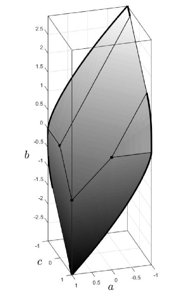
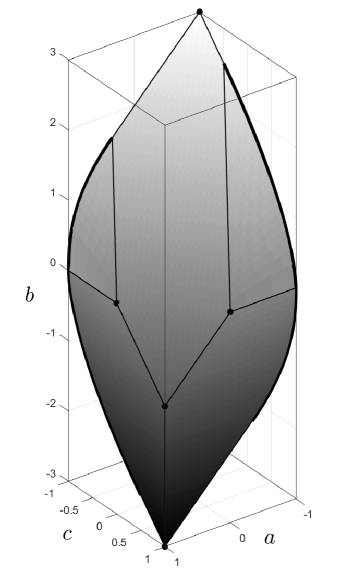
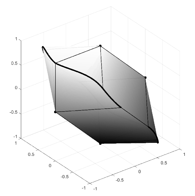
Theorem 3.4.
For every with , even, odd we have
The reader can find a representation of in Figure 15 for the case and .
Proof.
According to (1.2) we have that
which allows us to focus our efforts on the case where . As a matter of fact we can assume that .
Observe that any two norms and coincide on a linear space if and only if for every such that . Since the mappings can be easily proved to be concave using elementary differential calculus, the centrally symmetric set
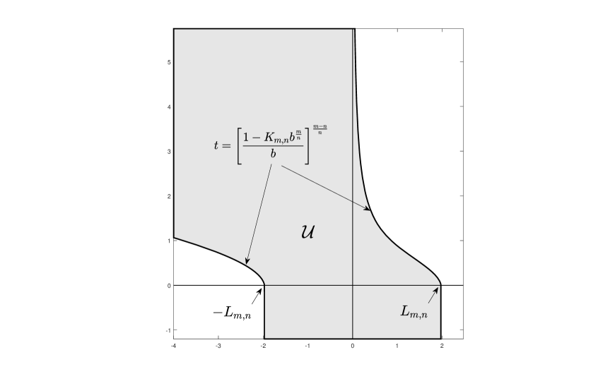
must be the unit sphere of a norm in . Hence, in order to prove that we just need to show that . Actually it suffices to show that due to the symmetry of with respect to the plane . Let us take , that is
We will study separately the five cases , , and .
Case 1:
From Lemma 3.3 we have that
Then according to (2.8) and the fact that
it follows that
In the last two steps we took into consideration that and that whenever .
Case 2:
By symmetry, and . Then, using the previous case
Case 3:
From Lemma 3.3 we have that
Then according to (2.8) and the fact that
it follows that
In the last two steps we took into consideration that and that whenever .
Case 4:
By symmetry, and . Then, using the previous case
Case 5:
4. The extreme points of
The parametrization of found in Theorem 3.4 together with the fact that most of the surfaces that take part in the graph of are ruled surfaces help tremendously to localize the extreme points of . This is addressed in the main result of this section.
Theorem 4.1.
Let be positive integers with , even and odd. Then consists of the points
and
where , is the positive number and is the curve from Lemma 3.1.
Proof.
First we show that the graph of restricted to is a ruled surface (to recall, the function is defined in (3.3), and the region is illustrated in Figure 12). Due to the symmetry of and , we just need to prove this by restricting to . Consider the lines in the plane that pass though and have slope with , where as in Lemma 3.1. The equation of each of these lines is given by . Let be the intersection point of and the curve . Obviously, the segments that join and , namely
cover the whole set as ranges over the interval . Also, restricted to is linear since, by (3.4)
for .
A similar argument reveals that the graph of restricted to is a ruled surface as well. In this case we have to consider the straight lines passing through in the plane with slope . The equation of each of those lines is . Let be the intersection point of and the curve or . Again, the segments that join and cover the whole as . Now it is easy to see that the restriction of to is affine since, by (3.8)
Finally, the graph of when restricted to is formed by two flat surfaces. We conclude that all the extreme points of must lie in the intersections of the graphs of when restricted to , with and . Some of these intersections produce, in their turn, segments. That is the case of the following intersections:
-
•
,
-
•
,
-
•
,
-
•
,
-
•
,
-
•
,
-
•
,
-
•
,
-
•
,
where , , , and . Here, is the point appeared in Lemma 3.1. Those segments can only contain extreme points of at their endpoints, that is, at , , , ,.
There are other intersections that provide both segments and curved lines. That happens in the following cases:
- •
Finally there are intersections that provide only curved lines:
-
•
with .
Therefore the extreme points of must lie among the points and or in the curves described in (4.1) and (4.2).
In the rest of the proof, we will say that a plane in is a supporting hyperplane to at if . To finish the proof we just have to construct supporting planes to at each point of the 8 curves represented in (4.1) and (4.2) and the four points and . The existence of such a plane would guarantee that is an extreme point of .
Starting with the points and , it can be easily seen that the planes
are supporting planes to at , , and respectively. Moreover, in fact there are infinitely many supporting hyperplanes at and . To prove this we will focus on the point since the other cases are similar. We just need to consider the family of hyperplanes passing through and parallel to the vectors and with (see Figure 16), that is,
Obviously for all .
As for the 8 curves in (4.1) and (4.2), it is enough to pay attention only to two cases due to the numerous existing symmetries. For instance take
-
(a)
with .
-
(b)
with .
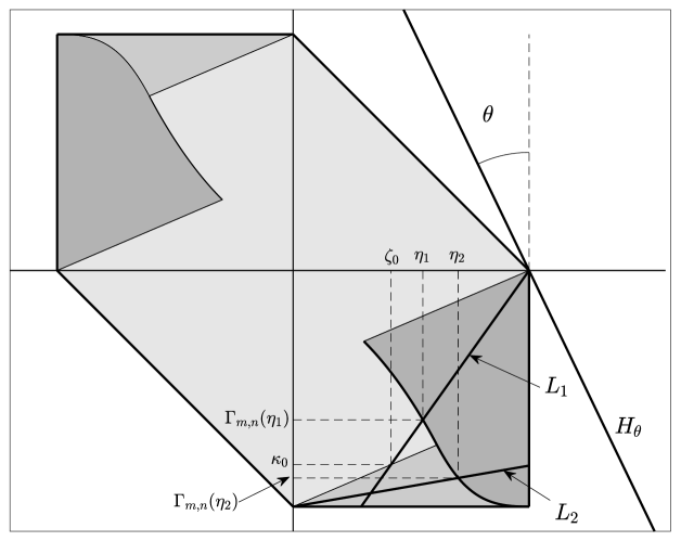
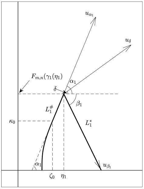
Let us study the curve appearing in (a). For simplicity we put
ending up with the curve
for . Taking an arbitrary , a supporting plane to at must be tangent to the curve at , or equivalently, parallel to . We need another vector to construct a plane passing through . Let with
The slope has been chosen so that the line in the -plane given by with passes through and . Consider the segment which results in intersecting the line and the projection of onto the plane (see Figure 16). Also, consider the plane that contains and is parallel to the axis. Obviously contains . Recall we have shown above in this proof that is linear on the segment joining and . Therefore the segment joining the points and is contained in the graph of restricted to . Since is affine on , the restriction of to is a segment, say . Therefore the graph of restricted to has two confluent segments at , namely and . We have represented this situation in Figure 17 where we have depicted the plane with the graph of the restriction of to . The remaining vector needed to construct a supporting hyperplane to at can be chosen in many ways. We call that vector and the resulting supporting hyperplane is:
The nature of and the index are revealed next. First consider two unitary vectors and parallel to and respectively. Here and are, respectively, the angles between and the plane and between and the plane (see Figure 17). Hence, the desired vector can be expressed in canonical coordinates of the plane as
with . Observe that we have not included the cases because whereas .
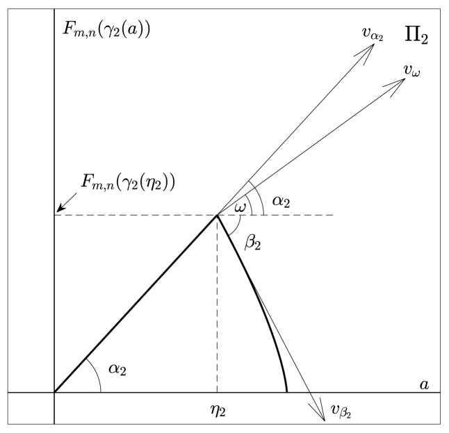
Finally we consider the curve in (b). Putting
we end up with the curve
for . Taking an arbitrary , a supporting plane to at must be tangent to the curve at , or equivalently, parallel to . We need another vector to construct a plane passing through . Let with
Notice that the slope has been chosen so that the segment in the -plane given by with passes through , starting at . Consider the plane that contains and is parallel to the axis. Obviously contains . Recall we have proved above in this proof that is linear on the segment joining and , as can be seen in Figure 18 where we have depicted the plane with the representation of the restriction of to . Let us call the segment joining and . The remaining vector needed to construct a supporting hyperplane to at can be chosen in many ways. If we call that vector , then the desired plane would be given by
The meaning of and the index will be explained in the rest of the proof. First consider the angle between the segment and the plane , that is,
Also let us choose a vector parallel to the tangent line to the graph of at , whose slope in the plane is given by
Hence, in canonical coordinates of the plane , could be expressed as
where
Finally, could be chosen to be any unitary vector between and in the plane , that is
with in coordinates of . Observe that we have not included the case because . We recommend to keep an eye on Figure 18 to follow the last part of the proof.
∎