Real-time Localization and Mapping
in Architectural Plans with Deviations
Abstract
Having prior knowledge of an environment boosts the localization and mapping accuracy of robots. Several approaches in the literature have utilized architectural plans in this regard. However, almost all of them overlook the deviations between actual “as-built” environments and “as-planned” architectural designs, introducing bias in the estimations. To address this issue, we present a novel localization and mapping method denoted as deviations-informed Situational Graphs or “diS-Graphs” that integrates prior knowledge from architectural plans even in the presence of deviations. It is based on Situational Graphs (S-Graphs) that merge geometric models of the environment with 3D scene graphs into a multi-layered jointly optimizable factor graph. Our diS-Graph extracts information from architectural plans by first modeling them as a hierarchical factor graph, which we will call an Architectural Graph (A-Graph). While the robot explores the real environment, it estimates an S-Graph from its onboard sensors. We then use a novel matching algorithm to register the A-Graph and S-Graph in the same reference, and merge both of them with an explicit model of deviations. Finally, an alternating graph optimization strategy allows simultaneous global localization and mapping, as well as deviation estimation between both the A-Graph and the S-Graph. We perform several experiments in simulated and real datasets in the presence of deviations. On average, our diS-Graphs outperforms the baselines by a margin of approximately in simulated environments and by in real environments, while being able to estimate deviations up to cm and .
Paper Video: https://www.youtube.com/watch?v=bgPm-sSXZ9g
I Introduction
Prior information from architectural plans can enhance the localization and mapping accuracy of mobile robots. Traditional techniques generally leverage only the metric information available in architectural plans, reducing its robustness in challenging environments. Recent approaches such as 3D scene graphs [1, 2] or Situational Graphs (S-Graphs) [3, 4], represent a robot’s environment in a compact and hierarchical manner, encoding high-level semantic abstractions (for example, walls and rooms) and their relationships (e.g., a set of walls forms a room). Herein, S-Graphs extend 3D scene graphs by merging geometric models of the environment generated by Simultaneous Localization and Mapping (SLAM) approaches with 3D scene graphs into a multi-layered jointly optimizable factor graph. This representation, combined with the prior information extracted from architectural plans, can be used to provide fast and efficient localization.
iS-Graphs [5] follows this direction and shows accurate localization over hierarchical factor graphs using prior information from architectural plans. iS-Graphs extracts elements such as wall-surfaces (planes), walls (two opposite wall-surfaces), rooms, doors, and floors from architectural plans to also model them as a hierarchical factor graph that we call an “Architectural Graph” (A-Graph) [5]. As a robot equipped with a LiDAR navigates the environment, it can detect features of the scene such as walls, rooms, and floors and model them online as an S-Graph. iS-Graphs then performs a hierarchical graph matching and merging to localize the robot within the A-Graph. However, its success is based on the assumption that there are no deviations between the S-Graph (“as-built”) and the A-Graph (“as-planned”). In reality, this is never the case, and the building elements exhibit certain deviations with respect to their planned geometries.
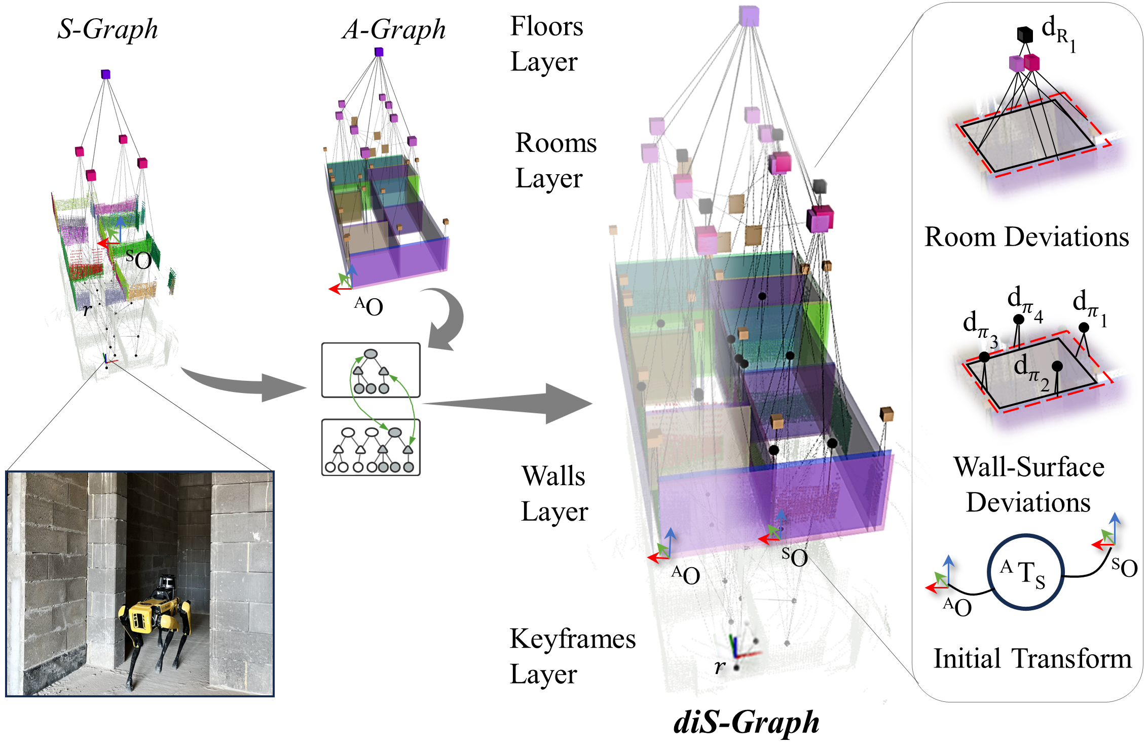
To address this issue, we present in this paper diS-Graphs (Fig. 1), a novel method capable of fusing “as-planned” and “as-built” data even in the presence of deviations. Given an A-Graph of a building, and while an S-Graph is being estimated online from a robot’s sensor readings, our approach simultaneously localizes the robot, maps the environment, and detects and estimates the deviations between the elements of “as-planned” and “as-built” environments. Therefore, our main contributions in this paper are:
-
•
A novel real-time localization and mapping algorithm based on Situational Graphs, integrating prior knowledge from architectural plans in the presence of deviations.
-
•
A two-stage matching algorithm based on graph structure, identifying deviations between S-Graphs and A-Graphs.
-
•
A novel deviation factor between the elements of the S-Graph and A-Graph, for simultaneously estimating global localization and deviations.
II Related Works
II-A Localization and Mapping with Precise Priors
Most localization and mapping techniques using prior information from architectural plans assume that the environments are built precisely according to the plans. One of the most commonly used localization techniques in 2D metric prior maps is Monte Carlo Localization (MCL) [6], [7] but it is not scaleable to large-scale complex environments. Boniardi et al [8] use a technique that scales to more complex environments by aligning a scan-based map with CAD-based floor plans. OGM2PGM [9] also scales to larger environments by converting the 2D floor plan to an occupancy grid map (OGM) and using a pose-graph map (PGM) to localize the robot. UKFL [10] further enhances the localization accuracy using an unscented Kalman filter to localize the robot in 3D metric meshes. Recent techniques such as [11] exploit neural networks to localize the robot using an implicit neural representation of the floor plans. All of the above mentioned techniques primarily rely on geometric information, not using any possible semantic information available in the architectural plans, limiting their ability to reason about the environment beyond geometric features. In addition, inaccuracies or outdated information in the floor plan can significantly affect the performance of these methods.
Semantic-based localization techniques, such as Mendez et al. [12] use semantic cues from architectural plans and sensor information to improve localization accuracy. Boniardi et al. [13] exploit the semantics of the room in architectural plans to do robot localization by matching the detected rooms from sensor data. Wang et al. [14] leverage prelabeled architectural features, such as wall intersections and corners, as landmarks in floor plans, and match them with detection from sensor data to jointly perform mapping and localization. Zimmerman et al. [15], [16] use high-level semantic information in floor plans, derived from object detection, along with geometric data from 2D LiDAR to perform long-term robot localization in floor plans. Huan et al. [17] convert architectural plans into semantically enriched point cloud maps, followed by a coarse-to-fine localization process using ICP. Gao et al. [18] used neural networks to detect vertical elements from floor plans to do LiDAR based localization. These methods are prone to inaccuracies due to misidentification and errors in the pose estimate of semantic elements. Moreover, they do not consider the topological relationship between different semantic elements for a more high-level understanding. Shaheer et al. [5] exploit the topological relationship between semantic elements to localize the robot with respect to architectural plans. However, all the above mentioned approaches assume no deviations between the architectural plans and the actual environment.
II-B Localization and Mapping with Imprecise Priors
Some recent works leverage imprecise floor plans for localization and mapping. Boniardi et al. [19] integrate mapping and localization techniques to take advantage of the information embedded in the CAD drawing, and the real-world observations acquired during navigation, which may not be reflected in the floor plan. Li et al. [20] presented a 2D LiDAR-based localization system in imprecise floor plans using stochastic gradient descent (SGD) with a scan matching algorithm. Chan et al. [21] presented a 2D LiDAR-based localization in floor plans that integrates SLAM with MCL. Blum et al. [22] use neural networks for feature segmentation and combine them with LiDAR data for localization in imprecise floor plans. Although these works can localize the robot in inaccurate floor plans, to the best of our knowledge, none of the existing works can localize the robot while simultaneously providing element-wise deviations between the “as-planned” and the “as-built” environments.
III System Architecture
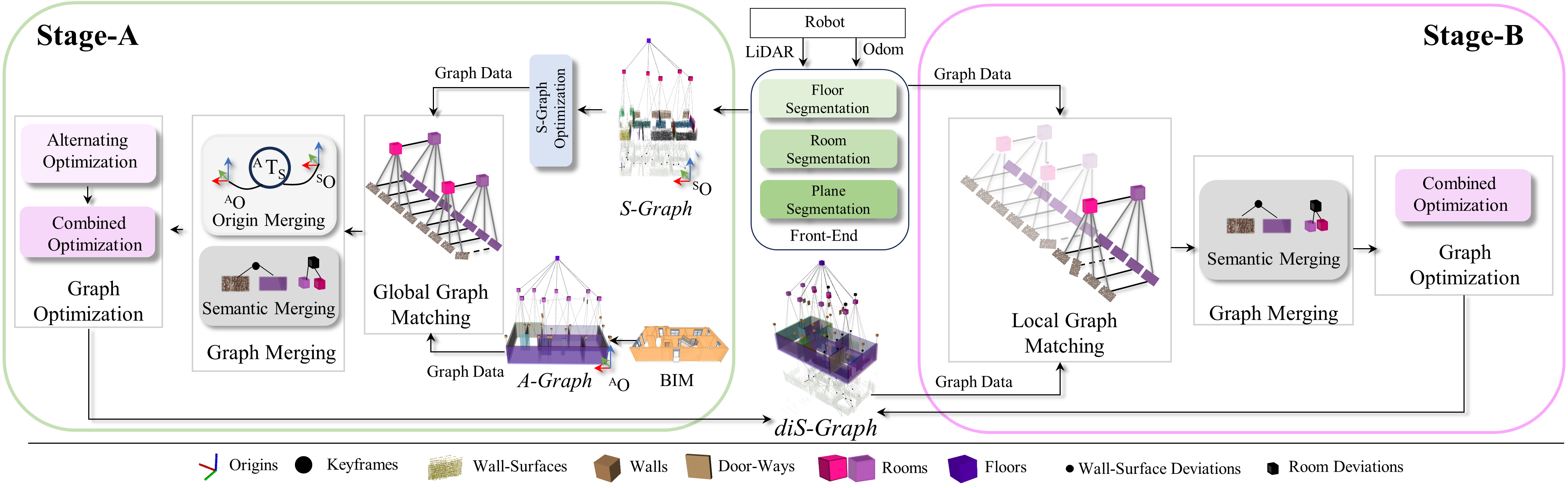
The overall system architecture of our approach is shown in Fig. 2. The algorithm has two stages: Stage-A and Stage-B, each consisting of multiple processes. In Stage-A, the A-Graph created from the architectural plan is first matched and merged with the S-Graph created by a robot, and then optimized. Stage-A is executed only once to get the initial estimates of the transformation between the two graphs, and potential deviations between its elements. Stage-B is executed periodically, as the new semantic entities are detected by the robot, to match and merge with the A-Graph, until the robot finishes exploring the environment.
III-A Graph Structures
Architectural Graph (A-Graph). Three-layered hierarchical factor graph model of the geometry, semantics, and topology of an environment, generated from its architectural plan. It models the environment “as-planned” by the architect.
Situational Graph (S-Graph). Four-layered hierarchical optimizable factor graph built online from 3D LiDAR and odometry measurements [3], [4] which models the “as-built” environment. It also includes the keyframes in addition to the geometry, semantics, and topology of the environment.
Deviations Informed-Situational Graph (diS-Graph). The result of merging both graphs, estimating the transformation between them and accounting for potential deviations is what we call diS-Graph.
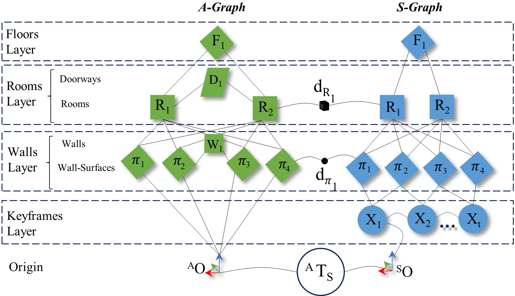
The layers of the graphs are depicted in Fig. 3 and can be detailed as follows:
Keyframes Layer. Only present in S-Graphs, this layer contains as nodes the robot poses in a global reference frame .
Walls Layer. In an A-Graph, this layer’s nodes encode two semantic entities, namely wall-surfaces and walls in the A-Graph global reference . We assume that each wall has two planar wall-surfaces with opposite orientations and the separation between them is equal to the width of the wall. In S-Graphs, this layer contains only the wall-surfaces extracted from 3D LiDAR scans. The keyframes that observe such wall-surfaces are linked to them through pose-plane constraints.
Rooms Layer. In an A-Graph, this layer also encodes two semantic entities, namely Rooms consisting of four wall-surfaces and Doorways . Two rooms constrain a doorway, and a room is constrained by four walls. In S-Graphs, this layer contains rooms comprising either four wall-surfaces or two wall-surfaces, and does not contain doorways.
Floors Layer. In both A-Graph and S-Graph this layer consists of a floor center node represented as , constraining all rooms present at that particular floor level. More details on the type of constraints between the different elements of the graphs can be found in [5].
III-B Graph Matching (Section IV)
The Global Graph Matching in Stage-A provides a unique match, when it exists, between the S-Graph and A-Graph at room and wall-surface levels, accounting for potential deviations. In Stage-B, the Local Graph Matching extends the previously matched elements in the diS-Graph with newly detected elements following an incremental approach.
III-C Graph Merging (Section. V)
Graph merging is performed for the candidates from the matching method from previous subsection. In Stage-A, graph merging involves the registration of the two graphs along with the semantic merging (wall-surfaces and rooms), with and explicit mapping of the deviation factors. Stage-B only performs the semantic merging that incorporates the newly observed entities with explicit deviation factors.
III-D Graph Optimization (Section. VI)
Graph optimization in Stage-A involves two steps of alternating optimization and combined optimization, while Stage-B involves only combined optimization (see Fig. 2). Alternating optimization estimates both the initial transformation between the origins of the S-Graph and the A-Graph, and possible deviations between the matched graph entities. Combined optimization performs a complete graph optimization given the initial global transformation and deviation estimates.
IV Graph Matching
Our graph matching extends the method presented in [5], summarized below for clarity.
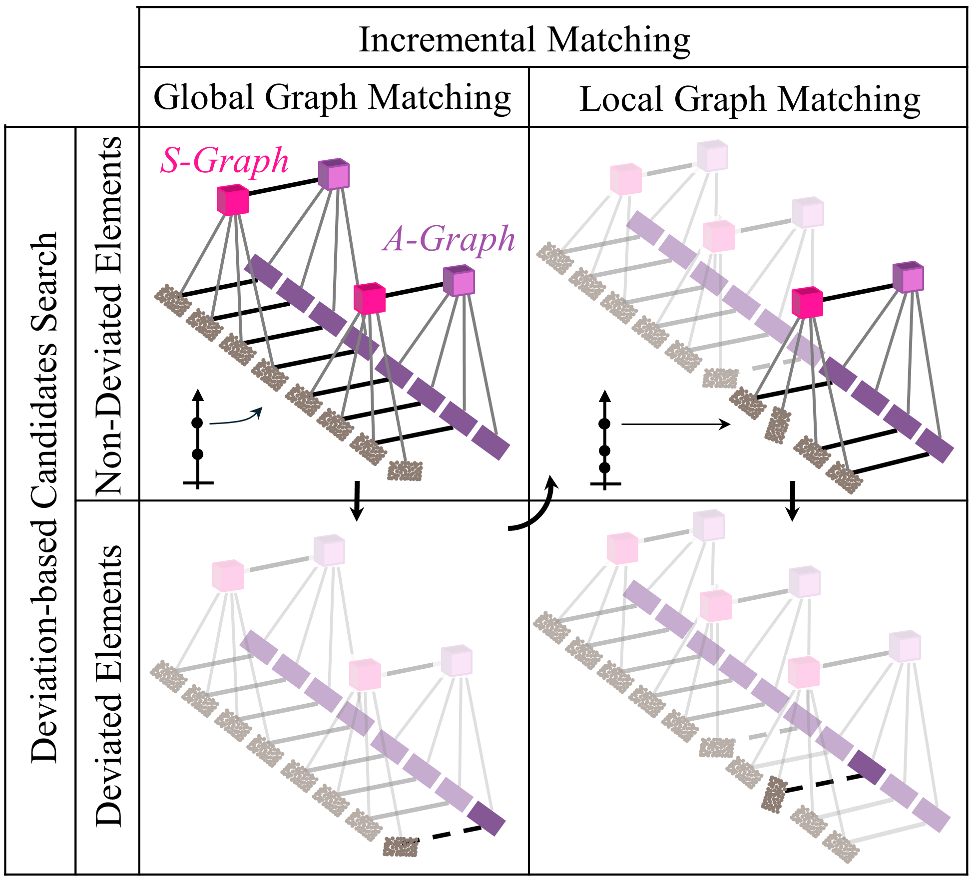
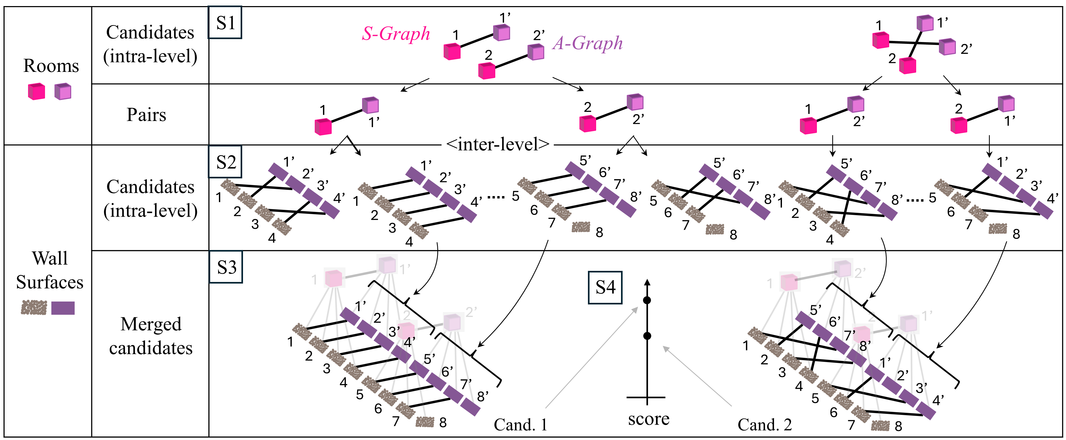
Background. In [5], a top-down potential candidate search between the A-Graph and S-Graph is performed by leveraging their hierarchical structures. To assess the overall consistency of each generated candidate, two verification steps are applied iteratively. First, the consistency of the node type and graph structure is verified. Second, geometric consistency (i.e. norm) is maintained over a certain consistency threshold [23]. The hierarchy of the structures is exploited through intra-level (i.e., same level) and inter-level (i.e. different levels) candidate consistency checks in the following steps (S) shown in Fig. 4(b). In S1, consistent room-to-room candidates are generated. In S2, and always consistent with its corresponding room pair, wall-surface-to-wall-surface candidates are generated. In S3, wall-surface candidates are merged with their room-level candidates. In S4, the overall geometrical consistencies of all the remaining candidates are compared. In the case where the score of the best candidate is higher than the second by a certain threshold, it is selected as the final unique match.
It is worth noting that symmetries may occur due to a lack of information as the robot has not visited the whole environment and thus the algorithm requires more information to provide a unique match, or when a large part of a building is symmetric and a unique match could never be found.
IV-A Deviation-based Candidates Search
The presence of deviations generates geometric inconsistencies that affect the aforementioned candidates’ checks. Concretely, a deviation in the position of a wall-surface implies a slight deviation in the center of its parent room as well. To handle this, we propose a two-stage search algorithm where we first search for non-deviated wall-surfaces followed by the inclusion of those that are deviated.
Non-Deviated Elements Search (Fig. 4(a) first row). To handle potential deviations, our method relaxes the matching criteria by decreasing the consistency thresholds at each level. First, we apply relaxed consistency thresholds for the generation of room-to-room and room-to-wall-surface match candidates, to account for the induced room-center inconsistencies. Then, to exclude deviated wall-surfaces, we increase the threshold for wall-surface-to-wall-surface candidates.
Deviated Elements Detection (Fig. 4(a) second row). To identify the deviated wall-surfaces which were not matched in the first stage but are connected to already matched rooms, we decrease the consistency threshold at wall-surface-to-wall-surface level.
To further speed up the candidate search, we incorporate the following information: Orphan Wall-Surfaces: We utilize wall-surfaces in the S-Graph without a parent room for the assessment of the geometrical consistency of the final match candidates at the wall-surface level. Ground Orientation: We exploit the ground plane normal in the A-Graph and the S-Graph, only allowing candidates with z-axis rotations.
Finally, the geometric consistency score provides a quantification of the probability of the deviation for each room and wall-surface, which is further used in the Graph Merging step (Section V).
IV-B Incremental Matching
To enhance the efficiency of the Graph Matching algorithm in [5], we propose an incremental approach with two stages (associated with stages A and B of the systems architecture of Fig. 2), namely Global Graph Matching (Fig. 4(a) left) and Local Graph Matching (Fig. 4(a) right), each executing the two previously described deviation-based candidate search stages. Until a first unique match has been found, the Global Graph Matching is executed for every new observation in the S-Graph. Afterward, the Local Graph Matching is executed every time the diS-Graph is updated with newly observed rooms and wall surfaces. Here, already-matched elements are excluded from candidate generation, and each assessment of intra-level consistency considers the previously matched elements at the corresponding level.
V Graph Merging
Origin Merging. We first merge the origins of two graphs by introducing a transformation factor . The cost function is defined as:
| (1) |
Here and are the origins of the A-Graph and S-Graph respectively, and is the transformation between them. stands for the covariance of the cost, and it is always assigned a high value to estimate the transformation factor accurately.
Semantic Merging. Next, we associate the wall-surfaces and rooms of the A-Graph and the S-Graph. To account for and estimate deviations between the two graphs, we introduce deviation factors in graph merging as follows:
Room Merging: To estimate the deviation in the pose of an associated room between the two graphs, we define a deviation factor between the two rooms as , where the cost function is defined as:
| (2) |
Here and are rooms of A-Graph and S-Graph, each consisting of a set of four wall-surfaces. is the covariance associated with the cost function depending on the probability of deviation estimated by the matching of the graph (Section IV). Rooms with a higher probability of deviation assigned by graph matching have a higher covariance assigned to their cost function than rooms with lower deviation probability. If all matched rooms have the same deviation probability, they are assigned lower uniform covariances.
Wall-Surface Merging: After associating the rooms of the A-Graph and the S-Graph, we then associate the wall-surfaces of the associated rooms. We define the deviation factor between two wall surfaces as . The cost function to estimate the deviation value is defined as:
| (3) |
Here , where and are the normal orientation and distance of a plane in the A-Graph. Similarly, is a plane of the S-Graph with respect to the S-Graph origin. is the covariance associated with the cost function. Like rooms, wall-surfaces with a higher deviation are assigned higher covariances, and the ones with a lower deviation are assigned lower uniform covariances.
VI Graph Optimization
When the robot starts navigating the environment having a prior A-Graph, it also generates in real-time an S-Graph. The overall state at time can be defined as:
| (4) |
where are the robot poses at selected keyframes in the S-Graph frame of reference, are the plane parameters of the and wall-surfaces of the S-Graph and A-Graph respectively, contains the parameters of the and four-wall rooms of the S-Graph and A-Graph respectively. are the parameters of the two-wall rooms in the S-Graph. contains the parameters of doorways of the A-Graph, are the floors levels, and models the drift between the odometry frame and the S-Graph reference frame . If at time there is no match obtained between the A-Graph and S-Graph we perform single S-Graph optimization as explained in [4].
Alternating Optimization. Alternating optimization is further performed in two steps as follows:
Transformation Estimation: Upon receiving the match (Section. IV) and performing graph merging (Section. V), we augment our global state with additional transformation factor . represents the transformation between the origins of the A-Graph and the S-Graph and add a factor between the two origins of the graph. It is important to note that at this stage, the wall-surface and room entities with possible deviation are not included for estimating .
Deviation Estimation: After optimizing we already have an initial guess of the transformation between the A-Graph and the S-Graph, and we can incorporate the deviated wall-surface and room entities into the graph with appropriate deviation factors. Our state then becomes where are the deviation factors between wall-surfaces and are the deviation factors between rooms. When optimizing we keep constant to obtain a good initial estimation of the deviation between the matched deviated entities.
Combined Optimization. Finally, after getting the initial estimates of the transformation between the origins and the deviations between the semantic entities, we optimize the whole state to simultaneously estimate the position of each semantic entity, deviations, and the transformation between the two graphs.
VII Experimental Evaluation
VII-A Methodology
Setup. We evaluated our algorithm in both simulated and real environments. Both simulated and real experiments were performed using a laptop computer with an Intel i9-11950H (8 cores, 2.6 GHz) with 32 GB of RAM.
Baselines. We have selected the following LiDAR-based baselines for comparisons due to their suitability, their reported results, and the availability of their code: AMCL [6], UKFL [10], OGM2PGM [9], IR-MCL [11], and iS-Graphs [5]. As each baseline takes a different map input for localization, we used 2D occupancy grid maps for AMCL and OGM2PGM, 3D meshes for UKFL and IR-MCL, and A-Graphs for iS-Graphs and our method diS-Graphs, respectively.
Simulated Datasets. We validate the algorithms in five simulated datasets named SE1 to SE5. To record the datasets, we use Gazebo physics simulator to recreate the robot, its sensors (LiDAR), and the 3D indoor environments obtained from actual architectural plans. We report the absolute trajectory error (ATE) compared with the available ground truth trajectory. We also report the localization convergence success rate of all methods.
Real Datasets. We collected data with a legged robot equipped with a Velodyne VLP-16 LiDAR, at five different construction sites (RE1 to RE5), with existing architectural plans. In real experiments, we report the Root Mean Square Error (RMSE) of the estimated 3D maps against the non-deviated 3D maps from the architectural plan. Furthermore, we report all methods’ convergence rates and convergence and computation times.
Deviations. Note that, given the absence of actual ground truth deviations in a real environment with respect to the plans, we explicitly deviate the wall-surfaces entities in the architectural plans to have a ground truth estimate of the deviations for both simulated and real datasets. For all datasets, we performed five separate tests introducing uniform random wall-surface deviations in architectural plans ranging from to in translation, and and in rotations.
Ablation. We conducted ablation studies on two key components of our algorithm. 1. Covariance assignment: As mentioned in the graph matching and graph merging (Section. IV & V), we assign covariances to the deviation factors of the semantic elements, based on their deviation likelihood. Here, we analyze the effect of assigning equal covariances, referred to as uniform covariances (UC), to both deviated and non-deviated elements. 2. Alternating optimization: In graph optimization (Section. VI) we discuss the use of alternating optimization for simultaneous localization and deviation estimation. Here, we study the performance when using only a single optimization cycle (SO).
VII-B Results and Discussion
Absolute Trajectory Error. Table I shows the ATE for all baselines and our diS-Graphs. Our method outperforms all baselines. Specifically, it shows an error reduction of around compared to AMCL, compared to OGM2PGM, compared to IR-MCL, compared to UKFL, and a reduction of over iS-Graphs, which uses architectural plans but assumes no deviations.
| Dataset | ||||||
| Method | ATE [cm] | |||||
| SE1 | SE2 | SE3 | SE4 | SE5 | Avg. | |
| AMCL [6] | 17.2 | 20.1 | 22.4 | 19.9 | ||
| UKFL [10] | 12.6 | 15.3 | 8.7 | 11.1 | 9.1 | |
| OGM2PGM [9] | 15.2 | 18.1 | 10.7 | 10.3 | 14.3 | 13.7 |
| IR-MCL [11] | 14.7 | 6.4 | 9.6 | 28.4 | 18.8 | 15.5 |
| iS-Graphs [5] | 5.4 | 6.7 | 16.6 | 4.6 | 9.5 | 8.5 |
| diS-Graphs (UC) | 6.2 | 7.3 | 13.7 | 8.4 | 8.6 | 8.8 |
| diS-Graphs (SO) | 4.4 | 6.1 | 15.2 | 7.7 | 6.2 | 7.9 |
| diS-Graphs (Ours) | 3.3 | 4.1 | 6.4 | 4.4 | 5.7 | 4.8 |
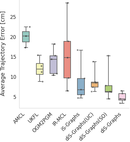
Fig. 6(a) summarizes the ATE performance of all the baseline algorithms. AMCL shows the highest median ATE and a relatively narrow distribution, indicating consistently high error rates. UKFL and OGM2PGM demonstrate moderate performance with similar median ATEs, although OGM2PGM shows a wider range of errors. IR-MCL exhibits the largest variability, suggesting inconsistent performance in different scenarios. Our diS-Graphs shows the lowest median ATE and the most compact distribution, indicating consistently low error rates under various conditions. This shows that the addition of explicit deviation factors between semantic elements reduces not only the ATE but also its variance.
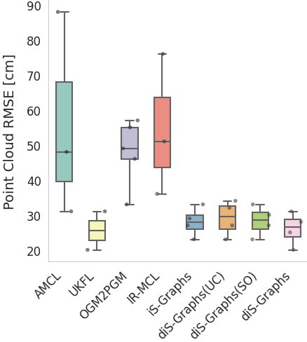
Pointcloud Alignment Error. Table II shows the RMSE of the point clouds with respect to the ground truth for all methods and ours. In case of deviations in construction from the plans, diS-Graphs shows better accuracy than AMCL, better than OGM2PGM, better than IR-MCL, and better than iS-Graphs. Although UKFL’s average error is equal to diS-Graphs’, it has a very low convergence rate (see Table III) rendering the comparison unfair. Moreover, it cannot estimate the deviations between “as-planned” and “as-built” environments. Fig. 6(b) summarizes the performance of all algorithms in real environments. AMCL exhibits the highest median and widest interquartile range, indicating greater variability in performance. IR-MCL presents a large spread of results, while OGM2PGM shows moderate performance with a smaller range of variability compared to AMCL and IR-MCL. UKFL and diS-Graphs show the lowest median RMSE, suggesting superior accuracy. Because of our simultaneous estimation of deviations and initial transformation, we can not only simultaneously globally localize the robot but also estimate the deviations between semantic elements of “as-planned” and “as-built” environments moreover improving the overall mapping accuracy compared to other algorithms.
| Dataset | ||||||
| Method | Point Cloud RMSE [cm] | |||||
| RE1 | RE2 | RE3 | RE4 | RE5 | Avg | |
| AMCL[6] | 0.48 | 0.88 | 0.31 | 0.56 | ||
| UKFL [10] | 0.31 | 0.20 | 0.26* | |||
| OGM2PGM[9] | 0.46 | 0.57 | 0.33 | 0.49 | 0.55 | 0.48 |
| IR-MCL[11] | 0.51 | 0.76 | 0.36 | 0.54 | ||
| iS-Graphs [5] | 0.27 | 0.29 | 0.23 | 0.33 | 0.28 | |
| diS-Graphs (UC) | 0.27 | 0.32 | 0.23 | 0.34 | 0.29 | |
| diS-Graphs (SO) | 0.27 | 0.30 | 0.23 | 0.33 | 0.28 | |
| diS-Graphs (ours) | 0.25 | 0.28 | 0.20 | 0.31 | 0.26 | |
-
•
* Omitted due to low convergence.
Convergence Rate. In terms of localization convergence rate in simulated environments (Table III) our approach shows a convergence rate better than AMCL, better than UKFL and better than OGM2PGM. Although the convergence rate of our algorithm is on par with that of IR-MCL, IR-MCL shows inconsistent performance in terms of ATE. We observed that since AMCL and UKFL rely heavily on the initial estimate of the robot’s starting position, their convergence rate is affected in environments with complex geometries, whereas the accuracy of OGM2PGM degrades in symmetric environments. IR-MCL, on the other hand, converges on most datasets but requires the model to be trained on every new dataset.
Table III shows the localization convergence rate in real environments. Our method shows the best convergence rate of all algorithms in four real environments (RE1-RE4) because of its ability to detect deviated elements in the environment. Our algorithm fails only in RE5 given the fact that the algorithm could not detect enough rooms in the environment to perform the graph matching.
| Dataset | ||||||||||
| Convergence Rate [%] | ||||||||||
| Method | SE1 | SE2 | SE3 | SE4 | SE5 | RE1 | RE2 | RE3 | RE4 | RE5 |
| AMCL [6] | 0 | 100 | 0 | 80 | 20 | 80 | 100 | 100 | 0 | 0 |
| UKFL [10] | 80 | 80 | 0 | 40 | 80 | 60 | 0 | 60 | 0 | 0 |
| OGM2PGM [9] | 80 | 100 | 100 | 80 | 80 | 60 | 80 | 100 | 60 | 80 |
| IR-MCL [11] | 100 | 100 | 100 | 20 | 100 | 60 | 100 | 20 | 0 | 0 |
| iS-Graphs [5] | 60 | 20 | 100 | 80 | 100 | 60 | 20 | 40 | 60 | 0 |
| diS-Graphs | 100 | 100 | 100 | 100 | 100 | 100 | 100 | 100 | 100 | 0 |
| Dataset | ||||||||||
| Convergence Time [s] | Computation Time [ms] | |||||||||
| Method | RE1 | RE2 | RE3 | RE4 | RE5 | RE1 | RE2 | RE3 | RE4 | RE5 |
| AMCL [6] | 24 | 89 | 29 | 2 | 2 | 2 | ||||
| UKFL [10] | 126 | 8 | 104 | 119 | ||||||
| OGM2PGM [9] | 16 | 38 | 27 | 35 | 79 | 2 | 2 | 2 | 2 | 2 |
| IR-MCL [11] | 16 | 26 | 13 | 92 | 90 | 89 | ||||
| iS-Graphs [5] | 155 | 101 | 78 | 139 | 57 | 78 | 78 | 64 | ||
| diS-Graphs | 81 | 43 | 46 | 139 | 56 | 77 | 76 | 70 | ||
| Seq. Len. [s] | 657 | 170 | 488 | 657 | 559 | 657 | 170 | 488 | 657 | 559 |
Convergence and Computation Time. Table IV shows the convergence and computation time for each algorithm. The computation time is the time used for each pose update. On average, the computation time of our algorithm is the best compared to other 3D algorithms, showing its real-time performance. OGM2PGM and AMCL have the best computation time because, unlike others, they process 2D information. The convergence time is the time it takes the algorithm to globally localize. IR-MCL and OGM2PGM have the best convergence time. iS-Graphs and diS-Graphs have considerably longer convergence times because they need to detect a certain number of rooms in the environment for graph matching to find a unique match. In addition, the previous version of graph matching struggled to resolve symmetries during the matching process, resulting in longer convergence times. However, the modifications in the graph matching algorithm (Section IV) proposed in this work improve the symmetry resolution ability and reduce the convergence time by almost .
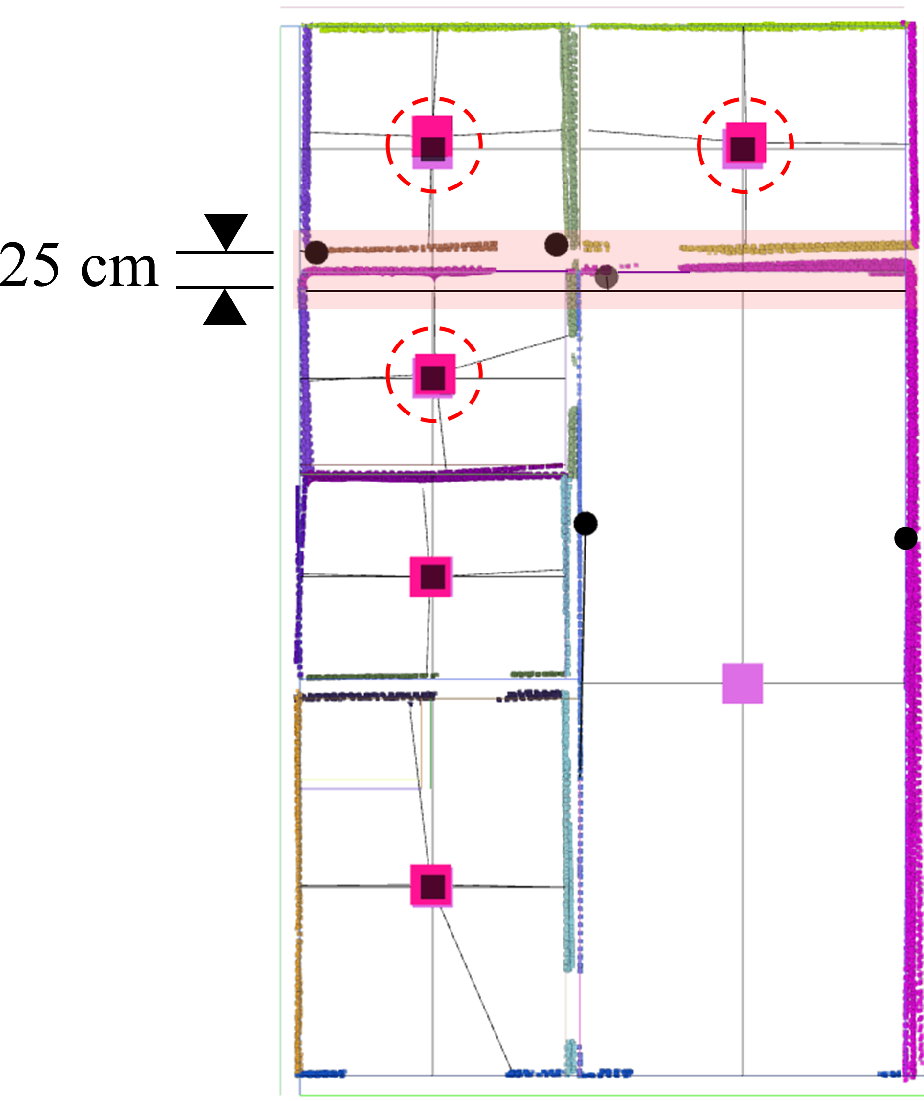
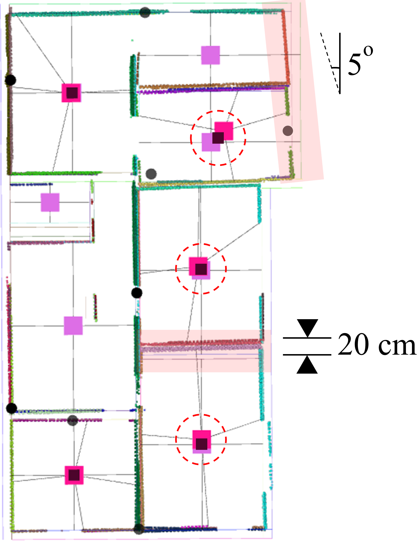
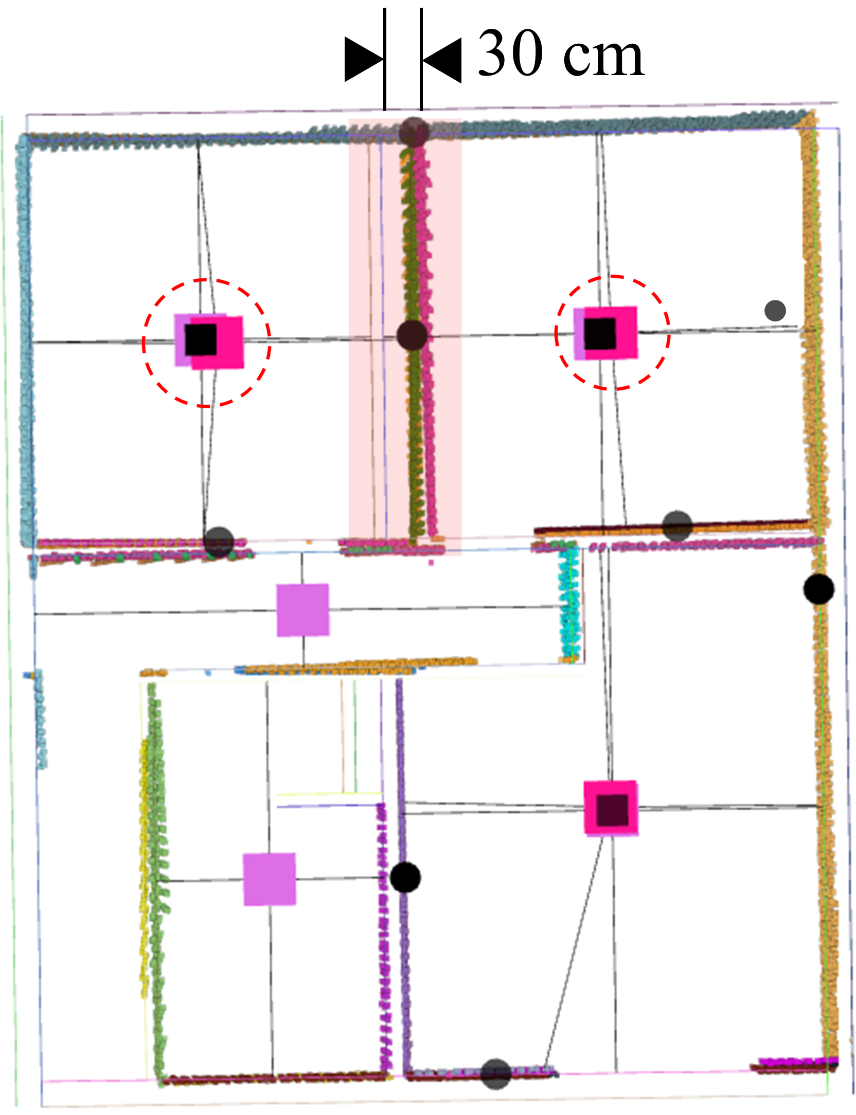
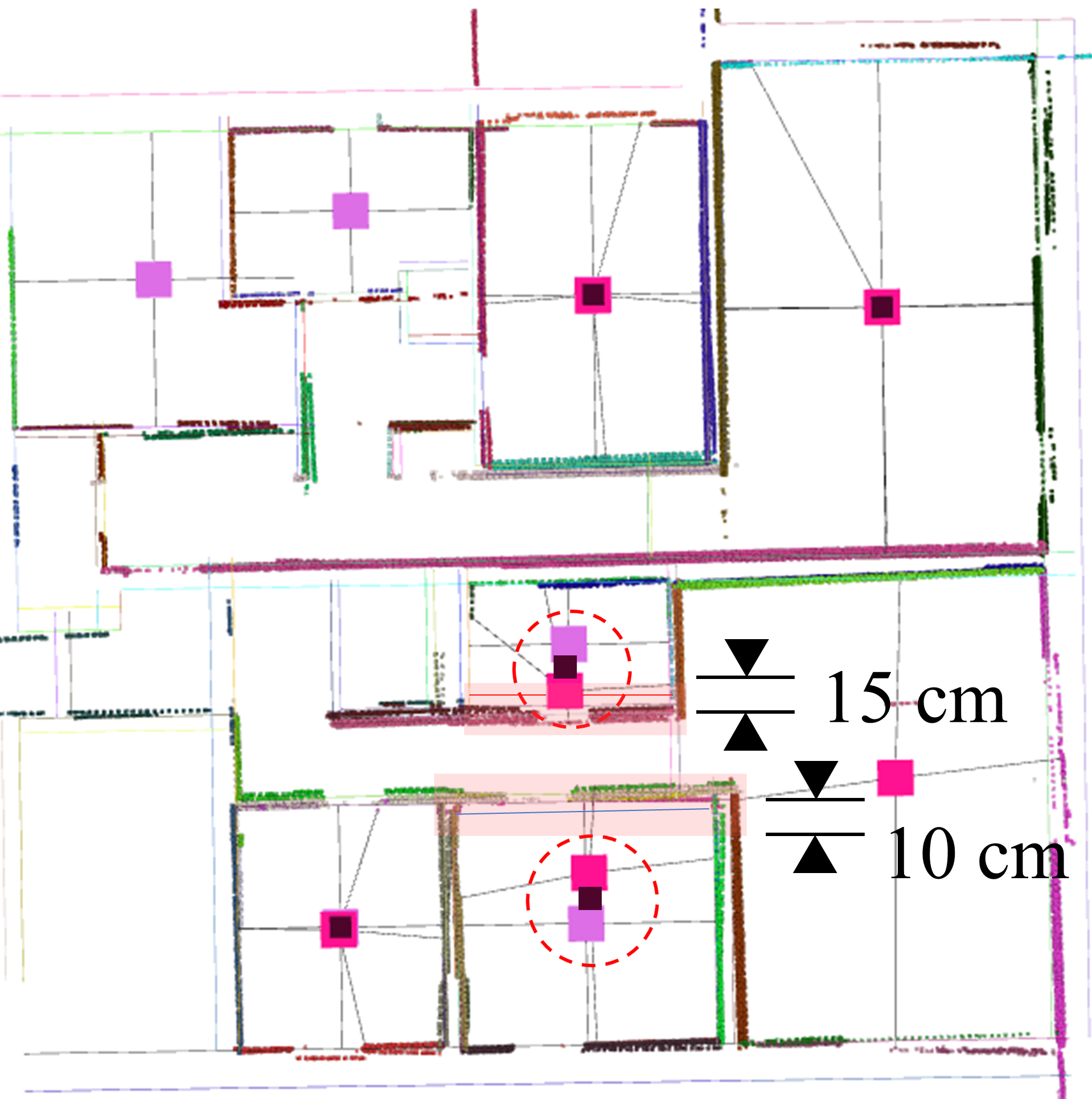
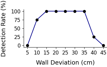
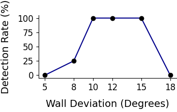
Deviation Estimation. Fig. 7 shows the amount of deviation our algorithm can correctly estimate in real environments. The accuracy level of our LiDAR is [24]. Considering that of the data falls within of the mean, and the fact that we are trying to estimate the deviations as well as transformation between the two graphs simultaneously, we can only accurately estimate the deviations greater than . The maximum translational and rotational deviation in wall-surfaces our algorithm can detect accurately is and respectively. Fig. 5 shows several qualitative results from our diS-Graphs method for real experiments. The robot can successfully localize, map, and estimate deviations in these environments. Note that we only show the rooms and walls for better understanding, and all the other semantic elements and the robot are not shown. We do not show RE5 in Fig. 5, as the robot could not localize itself in this sequence.
Ablation Study. Table I shows that associating ‘uniform covariance’ in simulated datasets (diS-Graphs (UC)) the algorithm cannot differentiate between deviated and non-deviated elements which results in poor pose estimation. In some cases, the use of uniform covariances results in even worse performance than iS-Graphs. Similarly, when using single optimization (diS-Graphs (SO)) instead of alternating optimization, the algorithm cannot differentiate between the transformation between two graphs and the deviations between their elements, resulting in higher ATE as shown in Table I.
Table II shows the ablation of uniform covariances and single optimization in real-world datasets. Using uniform covariances (diS-Graphs (UC)) and single optimization (diS-Graphs (SO)) results in lower mapping accuracy due to the algorithm’s inability to accurately map the deviated elements and differentiate between initial transformation and deviations simultaneously.
VIII Conclusions and Future Work
In this paper, we present our work on real-time localization and mapping in architectural plans with deviations while simultaneously estimating deviations between structural elements (specifically walls and rooms) of “as-planned” and “as-built” environments. Our work demonstrates higher localization accuracy in simulated environments, and higher mapping accuracy in real environments, and more robust performance in the presence of deviations between “as-planned” and “as-built” environments, compared to the best-performing existing method in the literature. Additionally, our algorithm provides an estimate of existing deviations up to in translation and in rotation.
Our algorithm is limited by the need to have enough distinctive semantic elements (i.e. wall-surfaces and rooms) to provide a unique match. As future work, we plan to add the ability to detect and match more semantic elements, which will translate into an improvement in the convergence rate and deviation detection range. Moreover, to gain flexibility, we plan to improve the matching process by adding the ability to detect rooms consisting of more than four walls.
References
- [1] I. Armeni, Z.-Y. He, A. Zamir, J. Gwak, J. Malik, M. Fischer, and S. Savarese, “3d scene graph: A structure for unified semantics, 3d space, and camera,” in 2019 IEEE/CVF International Conference on Computer Vision (ICCV).
- [2] N. Hughes, Y. Chang, and L. Carlone, “Hydra: A real-time spatial perception system for 3d scene graph construction and optimization,” in Robotics: Science and Systems XVIII. Robotics: Science and Systems Foundation.
- [3] H. Bavle, J. L. Sanchez-Lopez, M. Shaheer, J. Civera, and H. Voos, “Situational graphs for robot navigation in structured indoor environments,” vol. 7, no. 4, pp. 9107–9114, IEEE Robotics and Automation Letters.
- [4] ——, “S-graphs+: Real-time localization and mapping leveraging hierarchical representations,” IEEE Robotics and Automation Letters, vol. 8, no. 8, pp. 4927–4934, 2023.
- [5] M. Shaheer, J. A. Millan-Romera, H. Bavle, J. L. Sanchez-Lopez, J. Civera, and H. Voos, “Graph-based global robot localization informing situational graphs with architectural graphs,” in 2023 International Conference on Intelligent Robots and Systems, pp. 9155–9162.
- [6] D. Fox, W. Burgard, F. Dellaert, and S. Thrun, “Monte carlo localization: Efficient position estimation for mobile robots,” Aaai/iaai, vol. 1999, no. 343-349, pp. 2–2, 1999.
- [7] M. Shaheer, H. Bavle, J. L. Sanchez-Lopez, and H. Voos, “Robot localization using situational graphs (s-graphs) and building architectural plans,” Robotics, vol. 12, no. 3, p. 65, 2023.
- [8] F. Boniardi, T. Caselitz, R. Kümmerle, and W. Burgard, “A pose graph-based localization system for long-term navigation in cad floor plans,” Robotics and Autonomous Systems, vol. 112, pp. 84–97, 2019.
- [9] M. V. Torres, A. Braun, and A. Borrmann, “Ogm2pgbm: Robust bim-based 2d-lidar localization for lifelong indoor navigation,” in ECPPM 2022-eWork and eBusiness in Architecture, Engineering and Construction 2022, 2023, pp. 567–574.
- [10] K. Koide, J. Miura, and E. Menegatti, “A portable three-dimensional LIDAR-based system for long-term and wide-area people behavior measurement,” vol. 16, no. 2, p. 1729881419841532.
- [11] H. Kuang, X. Chen, T. Guadagnino, N. Zimmerman, J. Behley, and C. Stachniss, “Ir-mcl: Implicit representation-based online global localization,” IEEE Robotics and Automation Letters, vol. 8, no. 3, pp. 1627–1634, 2023.
- [12] O. Mendez, S. Hadfield, N. Pugeault, and R. Bowden, “SeDAR - semantic detection and ranging: Humans can localise without LiDAR, can robots?” in 2018 International Conference on Robotics and Automation, pp. 6053–6060.
- [13] F. Boniardi, A. Valada, R. Mohan, T. Caselitz, and W. Burgard, “Robot localization in floor plans using a room layout edge extraction network,” in 2019 International Conference on Intelligent Robots and Systems, pp. 5291–5297.
- [14] X. Wang, R. J. Marcotte, and E. Olson, “GLFP: Global localization from a floor plan,” in 2019 International Conference on Intelligent Robots and Systems, pp. 1627–1632.
- [15] N. Zimmerman, T. Guadagnino, X. Chen, J. Behley, and C. Stachniss, “Long-term localization using semantic cues in floor plan maps,” IEEE Robotics and Automation Letters, vol. 8, no. 1, pp. 176–183, 2022.
- [16] N. Zimmerman, M. Sodano, E. Marks, J. Behley, and C. Stachniss, “Constructing Metric-Semantic Maps Using Floor Plan Priors for Long-Term Indoor Localization,” in International Conference on Intelligent Robots and Systems, Oct. 2023, pp. 1366–1372.
- [17] Y. Huan, L. Zhiyi, and Y. K.W.Justin, “Semantic localization on BIM-generated maps using a 3D LiDAR sensor,” Automation in Construction, vol. 146, p. 104641, 2023.
- [18] L. Gao and L. Kneip, “FP-loc: Lightweight and drift-free floor plan-assisted LiDAR localization,” in 2022 International Conference on Robotics and Automation, pp. 4142–4148.
- [19] F. Boniardi, T. Caselitz, R. Kummerle, and W. Burgard, “Robust LiDAR-based localization in architectural floor plans,” in 2017 International Conference on Intelligent Robots and Systems, pp. 3318–3324.
- [20] Z. Li, M. H. Ang, and D. Rus, “Online localization with imprecise floor space maps using stochastic gradient descent,” in 2020 International Conference on Intelligent Robots and Systems, pp. 8571–8578.
- [21] C. L. Chan, J. Li, J. L. Chan, Z. Li, and K. W. Wan, “Partial-map-based monte carlo localization in architectural floor plans,” in Social Robotics. Springer International Publishing, vol. 13086, pp. 541–552.
- [22] H. Blum, J. Stiefel, C. Cadena, R. Siegwart, and A. Gawel, “Precise robot localization in architectural 3d plans,” arXiv preprint arXiv:2006.05137, 2020.
- [23] P. C. Lusk, K. Fathian, and J. P. How, “Clipper: A graph-theoretic framework for robust data association,” in International Conference on Robotics and Automation, 2021, pp. 13 828–13 834.
- [24] C. L. Glennie, A. Kusari, and A. Facchin, “Calibration and Stability Analysis of the VLP-16 Laser Scanner,” vol. XL-3/W4, pp. 55–60.