Intuitionistic Fuzzy Generalized Eigenvalue Proximal Support Vector Machine

A. Quadir M. A. Ganaie M. Tanveer
Abstract

Generalized eigenvalue proximal support vector machine (GEPSVM) has attracted widespread attention due to its simple architecture, rapid execution, and commendable performance. GEPSVM gives equal significance to all samples, thereby diminishing its robustness and efficacy when confronted with real-world datasets containing noise and outliers. In order to reduce the impact of noises and outliers, we propose a novel intuitionistic fuzzy generalized eigenvalue proximal support vector machine (IF-GEPSVM). The proposed IF-GEPSVM assigns the intuitionistic fuzzy score to each training sample based on its location and surroundings in the high-dimensional feature space by using a kernel function. The solution of the IF-GEPSVM optimization problem is obtained by solving a generalized eigenvalue problem. Further, we propose an intuitionistic fuzzy improved generalized eigenvalue proximal support vector machine (IF-IGEPSVM) by solving the standard eigenvalue decomposition resulting in simpler optimization problems with less computation cost which leads to an efficient intuitionistic fuzzy-based model. We conduct a comprehensive evaluation of the proposed IF-GEPSVM and IF-IGEPSVM models on UCI and KEEL benchmark datasets. Moreover, to evaluate the robustness of the proposed IF-GEPSVM and IF-IGEPSVM models, label noise is introduced into some UCI and KEEL datasets. The experimental findings showcase the superior generalization performance of the proposed IF-GEPSVM and IF-IGEPSVM models when compared to the existing baseline models, both with and without label noise. Our experimental results, supported by rigorous statistical analyses, confirm the superior generalization abilities of the proposed IF-GEPSVM and IF-IGEPSVM models over the baseline models. Furthermore, we implement the proposed IF-GEPSVM and IF-IGEPSVM models on the USPS recognition dataset, yielding promising results that underscore the models’ effectiveness in practical and real-world applications. The source code of the proposed IF-GEPSVM and IF-IGEPSVM models are available at https://github.com/mtanveer1/IF-GEPSVM.

keywords:
Fuzzy scheme , Intuitionistic fuzzy , Support vector machine , Eigenvalue , Generalized eigenvalue proximal support vector machines.
journal: Elsevier
\affiliation

[inst1]organization=Department of Mathematics,addressline=Indian Institute of Technology Indore, city=Simrol, Indore, postcode=453552, country=India \affiliation[inst2]organization=Department of Computer Science and Engineering,addressline=Indian Institute of Technology Ropar, city=Punjab, postcode=140001, country=India

1 Introduction

Support vector machines (SVMs) [4] is one of the most successful machine learning tools for classification and regression. SVM is based on statistical learning theory and have been applied to numerous real-world problems such as bio-medicine [31], activity recognition [21], image processing [13], text categorization [20] and so on. The main idea of SVM is to seek an optimal plane by maximizing the margin between two parallel supporting hyperplanes. SVM solves one large quadratic programming problem (QPP), resulting in escalated computational complexity, which renders it less suitable for large-scale datasets. It also implements the structural risk minimization (SRM) principle, leading to improved generalization performance.

Although SVM has made significant strides in various fields, there remains considerable room for improvement. A notable obstacle for the SVM is the substantial computational intricacy involved in solving the QPP. Mangasarian and Wild [27] proposed the generalized eigenvalue proximal SVM (GEPSVM), to mitigate the adverse impact of high computational consumption. GEPSVM aims to find two non-parallel hyperplanes such that each hyperplane is closer to the samples in one class and far away from the samples in the other class by solving two generalized eigenvalue problems. In improved GEPSVM (IGEPSVM) [37], the standard eigenvalue decomposition replaces the generalized eigenvalue decomposition, leading to simpler optimization problems without the potential for singularity. Jayadeva et al. [19] proposed twin SVM (TSVM) to solve two smaller-sized QPPs to obtain two non-parallel hyperplanes. Compared with solving one entire QPP in SVM, making TSVM is four times faster than SVM [42]. Suykens and Vandewalle [39] introduced a variant of SVM known as the least squares support vector machine (LSSVM), to decrease the training cost. LSSVM solves system of linear equations by using a squared loss function instead of the hinge loss. In order to further diminish the training cost, Kumar and Gopal [22] introduced a twin variant of LSSVM known as the least square TSVM (LSTSVM). The computation time of LSTSVM is much less in comparison to TSVM. Several modified TSVM models have been proposed, each based on various considerations, including universum TSVM (UTSVM) [34], KNN weighted reduced universum for class imbalance learning [11], inverse free reduced universum TSVM for imbalanced data classification (IRUTSVM) [30], and elastic net TSVM and its safe screening rules (SSR-ETSVM) [45]. Other latest advanced models are detailed in [14, 15, 47, 32].

In real-world environments, the presence of noise and outliers necessitates careful consideration. SVM fails to find an optimal hyperplane when the support vectors are contaminated with noise or outliers, leading to suboptimal or inferior results. To mitigate the influence of noise and outliers, the pinball loss function is employed in SVM (pin-SVM) [17]. The $\epsilon$-insensitive zone is incorporated into the pin-SVM [17] to retain the sparsity of the model. Several variants of TSVM have been proposed to mitigate the influence of noise and outliers including $L_{1}$ norm LSTSVM (NELSTSVM) [12], general TSVM with pinball loss (pin-GTSVM) [41], twin parametric margin SVM with pinball loss (Pin-TSVM) [48], ramp loss K-nearest neighbor-weighted multi-class TSVM (RKWMTSVM) [44], multi-view universum TSVM with insensitive pinball loss (Pin-MvUTSVM) [26], universum TSVM with pinball loss function (Pin-UTSVM) [10], granular ball TSVM with pinball loss (Pin-GBTSVM) [35], and large scale pinball TSVM (LPTWSVM) [43]. In addition to different loss functions, fuzzy SVM (FSVM) [9, 2, 25] has been proposed, to alleviate the influence of noise and outliers. FSVM calculates the degree of membership function of an input sample based on its individual contribution. This approach enhances the generalization ability of SVMs and mitigates the influence of noise and outliers. Due to superior performance, FSVM has gained popularity in classification tasks and has found broader applications in various domains, including human identification [24], medical applications [29], credit risk evaluation [46], and so on. Furthermore, various variants of FSVM have emerged, including a novel fuzzy TSVM [3] and FSVM for regression estimation [38], which incorporates a novel fuzzy membership function for addressing two-class problems [40]. When assigning membership degrees to training points based on their distance from the respective class center, patterns closer to the class center contribute equally to learning the decision surface. However, this approach can lead to certain edge support vectors being incorrectly identified as outliers. Later on, Ha et al. [28] proposed an intuitionistic fuzzy SVM (IF-SVM), in which the influence of each training point on the learning of the decision surface is determined by two parameters: hesitation and degrees of membership. Rezvani et al. [36] introduced intuitionistic fuzzy TSVM (IF-TSVM), by incorporating the degree of membership and non-membership function to further reduce the impact of noise. IF-TSVM has large computational complexity as it solves two QPPs to obtain the optimal hyperplane. Also, IF-TSVM involves matrix inverse computation, which can become impractical in large-scale problems, and may potentially lead to singularity issues. To get motivated by the intuitionistic fuzzy membership scheme and superior performance of GEPSVM, in this paper, we propose intuitionistic fuzzy generalized eigenvalue proximal support vector machine (IF-GEPSVM) by solving the generalized eigenvalue problem in the intuitionistic fuzzy environment. A score, consisting of both membership and non-membership degrees, is assigned to each training instance. The degree of membership function is calculated by the distance between the samples and the corresponding class center while the non-membership functions leverage the statistical correlation between the count of heterogeneous samples to all the samples within their neighborhoods. This membership scheme allows the model to effectively handle outliers and noise that have trespassed in the dataset. To address concerns related to the singular value problem and further enhance the speed of obtaining optimal solutions, we propose intuitionistic fuzzy improved generalized eigenvalue proximal support vector machine (IF-IGEPSVM). IF-IGEPSVM solves two standard eigenvalue problems which resolve the singularity issues in IF-GEPSVM. The main highlights of this paper are as follows:

  • 1.

    We propose an intuitionistic fuzzy GEPSVM (IF-GEPSVM) and intuitionistic fuzzy IGEPSVM (IF-IGEPSVM). The score value based on the intuitionistic fuzzy number is assigned to each training sample according to their importance in learning the classifier.

  • 2.

    We provide rigorous mathematical frameworks for both IF-GEPSVM and IF-IGEPSVM, covering linear and non-linear kernel spaces. Training in the kernel space elevates the proposed models’ performance by effectively capturing intricate data patterns and complex relationships through non-linear transformations.

  • 3.

    We carried out experiments on artificial datasets and $62$ UCI and KEEL benchmark datasets from diverse domains. The experimental outcomes validate the effectiveness of the proposed IF-GEPSVM and IF-IGEPSVM models when compared to the baseline models.

  • 4.

    The proposed IF-GEPSVM and IF-IGEPSVM models undergo rigorous testing with the addition of noise to datasets. Results indicate that the proposed models exhibit robustness to noise and stability to resampling, highlighting their effectiveness under noisy conditions.

  • 5.

    As an application, we conducted an experiment on USPS recognition datasets, the numerical experimental demonstrates the superiority of the proposed IF-GEPSVM and IF-IGEPSVM models over the baseline models.

This paper is organized as follows: Section 2 discusses a brief overview of GEPSVM, IGEPSVM, and intuitionistic fuzzy membership schemes. Section 3 presents the formulation of the proposed IF-GEPSVM and IF-IGEPSVM models, respectively. Section 6 provides a detailed explanation of the experimental results. Finally, the conclusions and potential future research directions are given in Section 7.

2 Background

In this section, we first go through the architecture of GEPSVM and IGEPSVM along with mathematical formulation and intuitionistic fuzzy membership. Let $D=\{(x_{i},y_{i}),i=1,2,\ldots,m\},$ be the traning dataset where $y_{i}\in\{+1,-1\}$ represents the label of $x_{i}\in\mathbb{R}^{1\times n}$. Let us consider the input matrices $A$ $\in\mathbb{R}^{m_{1}\times n}$ and $B$ $\in\mathbb{R}^{m_{2}\times n}$ representing the data points of $+1$ class and $-1$ class respectively, where $m_{1}$ and $m_{2}$ represent the number of data samples belonging to the $+1$ and $-1$ class, with the total number of data samples being $m=m_{1}+m_{2}$. The number of features is denoted by $n$ and $e$ represents the vectors of ones of appropriate dimension.

2.1 Rayleigh Quotient

The Rayleigh quotient [33], denoted as $Q(N,y)$, is defined for a given real symmetric matrix $N\in\mathbb{R}^{m\times m}$ and a nonzero real vector $y\in\mathbb{R}^{m\times 1}$,

$$Q(N,y)=\frac{y^{T}Ny}{y^{T}y}.$$ (1)

The Rayleigh quotient, $Q(N,y)$, achieves its maximum (minimum) value, $\lambda_{max}$ ($\lambda_{min}$), when $y$ is equal to $\mu_{max}$ ($\mu_{min}$). Here, $\mu_{max}$ ($\mu_{min}$) refers to the eigenvector of the generalized eigenvalue problem $Ay=\lambda By$, which corresponds to the maximum (minimum) eigenvalue.

2.2 Generalized Eigenvalue Proximal Support Vector Machine (GEPSVM)

GEPSVM [27] generates a pair of non-parallel hyperplanes

$$w_{1}^{T}x+b_{1}=0,\hskip 14.22636pt\text{and}\hskip 14.22636ptw_{2}^{T}x+b_{2}=0,$$ (2)

such that each hyperplane is closer to the data sample of one class and it is farther from the data samples of another class. The optimization problem of GEPSVM is given by:

$$\underset{(w_{1},b_{1})\neq 0}{min}\hskip 5.69046pt\frac{\|Aw_{1}+e_{1}b_{1}\|^{2}+\delta\|\tbinom{w_{1}}{b_{1}}\|^{2}}{\|Bw_{1}+e_{2}b_{1}\|^{2}},$$ (3)

and

$$\underset{(w_{2},b_{2})\neq 0}{min}\hskip 5.69046pt\frac{\|Bw_{2}+e_{2}b_{2}\|^{2}+\delta\|\tbinom{w_{2}}{b_{2}}\|^{2}}{\|Aw_{2}+e_{1}b_{2}\|^{2}},$$ (4)

were $\delta>0$ is a regularization parameter. To make the notation simpler, we introduce $G=[A\hskip 5.69046pte_{1}]^{T}[A\hskip 5.69046pte_{1}]\in\mathbb{R}^{(n+1)\times(n+1)}$, $H=[B\hskip 5.69046pte_{2}]^{T}[B\hskip 5.69046pte_{2}]\in\mathbb{R}^{(n+1)\times(n+1)}$ are symmetric matrices, $z_{1}=[w_{1};\hskip 5.69046ptb_{1}]\in\mathbb{R}^{(n+1)}$, and $z_{2}=[w_{2};\hskip 5.69046ptb_{2}]\in\mathbb{R}^{(n+1)}$. By solving the following generalized eigenvalue problems to obtain the solution

$\displaystyle(G+\delta I)z_{1}=\lambda Hz_{1},\hskip 5.69046ptz_{1}\neq 0,$ (5)
$\displaystyle(H+\delta I)z_{2}=\lambda Gz_{2},\hskip 5.69046ptz_{2}\neq 0,$ (6)

where $I$ denotes an identity matrix of appropriate dimension.

Once the optimal values of $z_{1}$ and $z_{2}$ are obtained. The classification of a new input data point $x$ into either the class $+1$ or $-1$ can be determined as follows:

$\displaystyle class(x)=\underset{i\in\{1,2\}}{\arg\min}\frac{\lvert w_{i}^{T}x+b_{i}\rvert}{\|w_{i}\|}.$ (7)

2.3 Improved GEPSVM (IGEPSVM)

IGEPSVM [37] seeks to determine two non-parallel hyperplanes, with each having a small distance from its respective class and a large distance from the other class. IGEPSVM employs subtraction instead of a ratio to learn the non-parallel hyperplanes. The optimization problem of IGEPSVM is as follows:

$$\underset{(w_{1},b_{1})\neq 0}{min}\hskip 5.69046pt\frac{\|Aw_{1}+e_{1}b_{1}\|^{2}}{\|w_{1}\|^{2}+b_{1}^{2}}-\delta\frac{\|Bw_{1}+e_{2}b_{1}\|^{2}}{\|w_{1}\|^{2}+b_{1}^{2}},$$ (8)

and

$$\underset{(w_{2},b_{2})\neq 0}{min}\hskip 5.69046pt\frac{\|Bw_{2}+e_{2}b_{2}\|^{2}}{\|w_{2}\|^{2}+b_{2}^{2}}-\delta\frac{\|Aw_{2}+e_{1}b_{2}\|^{2}}{\|w_{2}\|^{2}+b_{2}^{2}},$$ (9)

where $\delta$ denotes the weight factor. Then the global optimal solution of IGEPSVM can be obtained by solving the following standard eigenvalue problems:

$\displaystyle(G+\eta I-\delta H)z_{1}=\lambda_{1}z_{1},$ (10)
$\displaystyle(H+\eta I-\delta G)z_{2}=\lambda_{2}z_{2}.$ (11)

After obtaining the optimal values of $z_{1}$ and $z_{2}$. The classification of a new input data point $x$ into either the class $+1$ or $-1$ can be determined as follows:

$\displaystyle class(x)=\underset{i\in\{1,2\}}{\arg\min}\frac{\lvert w_{i}^{T}x+b_{i}\rvert}{\|w_{i}\|}.$ (12)

2.4 Intuitionistic Fuzzy Membership Scheme

The concept of the fuzzy set was introduced by Zadeh [49] in 1965, and the intuitionistic fuzzy set (IFS) was subsequently proposed by Atanassov and Atanassov [1] as a means to address uncertainties. It enables a precise representation of situations through the utilization of current information and observations [16]. In IFS scheme, there are three parameters in an intuitionistic fuzzy number (IFN): the membership degree, non-membership degree, and degree of hesitation, which is denoted as $\nu(0\leq\nu\leq 1)$, $\mu(0\leq\mu\leq 1)$ and $\pi=1-\nu-\mu$ [36]. According to the intuitionistic fuzzy membership (IFM) scheme, every training sample is allocated an IFN, denoted as $(\mu,\nu)$. Finally, a score function is formulated based on $\mu$ and $\nu$ values to examine the presence of outliers within the dataset. The degree of membership and nonmembership function is expressed as follows:

  1. 1.

    Membership Function The membership function is defined as the distance between the sample and the corresponding class center within the feature space. The membership function of each $i^{th}$ training sample is defined as:

    $$\mu(x_{i})=\begin{cases}1-\frac{\|\psi(x_{i})-C^{+}\|}{r^{+}+\hskip 5.69046pt\gamma},&y_{i}=+1,\\ 1-\frac{\|\psi(x_{i})-C^{-}\|}{r^{-}+\hskip 5.69046pt\gamma},&y_{i}=-1,\end{cases}$$ (13)

    where $\gamma$ is a non-negative parameter, $\psi$ represents the feature (projection) mapping function, and $r^{+}(r^{-})$ are the radius of $+1$ $(-1)$ class given by

    $\displaystyle r^{+}=\underset{y_{i}=+1}{\max}\|\ \psi(x_{i})-C^{+}\|,\hskip 5.69046pt\text{and}\hskip 5.69046ptr^{-}=\underset{y_{i}=-1}{\max}\|\ \psi(x_{i})-C^{-}\|,$ (14)

    where $C^{+}(C^{-})$ are the center of $+1$ $(-1)$ class, respectively. The class center is defined as

    $\displaystyle C^{+}=\frac{1}{m_{1}}\sum_{y_{i}=+1}\psi(x_{i}),\hskip 5.69046pt\text{and}\hskip 5.69046ptC^{-}=\frac{1}{m_{2}}\sum_{y_{i}=-1}\psi(x_{i}),$ (15)

    here $m_{1}$ and $m_{2}$ are the number of $+1$ and $-1$ class samples, respectively.

  2. 2.

    Non-membership function The non-membership function for each training sample is defined as the proportion of heterogeneous points to the total number of points within its vicinity. Therefore, the nonmembership function is calculated as follows:

    $$\nu(x_{i})=(1-\mu(x_{i}))\eta(x_{i}),$$ (16)

    where the local neighborhood set $\eta(x_{i})$ is calculated as:

    $$\eta(x_{i})=\frac{|\{x_{j}|\|\psi(x_{i})-\psi(x_{j})\|\leq\beta,\,y_{j}\neq y_{i}\}|}{|\{x_{j}|\|\psi(x_{i})-\psi(x_{j})\|\leq\beta\}|},$$ (17)

    here $\beta$ is an adjustable non-negative parameter and $\lvert\cdot\rvert$ represents the cardinality.

  3. 3.

    Score of each training sample: The score function amalgamates the significance of membership and non-membership, and this can be calculated as:

    $$s_{i}=\left\{\begin{array}[]{lr}\mu_{i},&\nu_{i}=0,\\ 0,&\mu_{i}\leq\nu_{i},\\ \frac{1-\nu_{i}}{2-\mu_{i}-\nu_{i}},&\text{others}.\end{array}\right.$$ (18)

    Finally, the score matrix $S$ for the dataset $D$ is defined as: $S=diag\{s(x_{i})\hskip 2.84544pt|\hskip 2.84544pti=1,2,\ldots,m\}$.

We calculate the intuitionistic fuzzy membership scheme in high-dimensional space. It is essential to accurately compute the distance between data points in this high-dimensional feature space. This is where the kernel function becomes crucial, as it allows us to implicitly map data points into a higher-dimensional space without needing an explicit formula for the transformation. Specifically, the kernel function $k(x_{i},x_{j})=\psi(x_{i})^{T}\psi(x_{j})$ defines the inner product between the images of the data points $x_{i}$ and $x_{j}$ in the feature space. However, since we do not have an explicit representation of $\psi(x)$, calculating the direct distance between points is not straightforward. Theorems 1 and 2 provide a mathematical framework to compute the distances between the points and the distance between the point to the center in the kernel space effectively, ensuring that the intuitionistic fuzzy membership values are calculated accurately. Therefore, these theorems are not just for structure but are essential components that leverage the kernel function to calculate the intuitionistic fuzzy membership scheme in high-dimensional spaces accurately.

Theorem 1.

[16]: Let the kernel function is $K(x_{i},x_{j})$. Then, the inner product distance is given by:
$\|\psi(x_{i})-\psi(x_{j})\|=\sqrt{K(x_{i},x_{i})-2K(x_{i},x_{j})+K(x_{j},x_{j})}$.

Proof.
$\displaystyle\|\psi(x_{i})-\psi(x_{j})\|$ $\displaystyle=\sqrt{(\psi(x_{i})-\psi(x_{j})).(\psi(x_{i})-\psi(x_{j}))}$
$\displaystyle=\sqrt{(\psi(x_{i}).\psi(x_{i}))-(\psi(x_{i}).\psi(x_{j}))+(\psi(x_{j}).\psi(x_{j}))}$
$\displaystyle=\sqrt{K(x_{i},x_{i})-2K(x_{i},x_{j})+K(x_{j},x_{j})}.$

Theorem 2.

[16]: The Euclidean distance between the samples and the corresponding class center is represented by:
$\|\psi(x_{i})-C^{+}\|=\sqrt{K(x_{i},x_{i})-\frac{2}{m_{1}}\sum_{y_{j}=+1}K(x_{i},x_{j})+\frac{1}{m_{1}^{2}}\sum_{y_{i}=+1}\sum_{y_{j}=+1}K(x_{i},x_{j})}$,
$\|\psi(x_{i})-C^{-}\|=\sqrt{K(x_{i},x_{i})-\frac{2}{m_{2}}\sum_{y_{j}=-1}K(x_{i},x_{j})+\frac{1}{m_{2}^{2}}\sum_{y_{i}=-1}\sum_{y_{j}=-1}K(x_{i},x_{j})}$.

Proof.
$\displaystyle\|\psi(x_{i})-C^{+}\|$ $\displaystyle=\sqrt{(\psi(x_{i})-C^{+}).(\psi(x_{i})-C^{+})}$
$\displaystyle=\sqrt{(\psi(x_{i}).\psi(x_{i}))+(C^{+}.C^{+})-2(\psi(x_{i}).C^{+})}$
$\displaystyle=\sqrt{K(x_{i},x_{i})+\left(\frac{1}{m_{1}}\sum_{y_{i}=+1}\psi(x_{i})\right).\left(\frac{1}{m_{1}}\sum_{y_{i}=+1}\psi(x_{i})\right)-2\psi(x_{i})\left(\frac{1}{m_{1}}\sum_{y_{j}=+1}\psi(x_{i})\right)}$
$\displaystyle=\sqrt{K(x_{i},x_{i})+\frac{1}{m_{1}^{2}}\sum_{y_{i}=+1}\sum_{y_{j}=+1}K(x_{i},x_{j})-\frac{2}{m_{1}}\sum_{y_{j}=+1}K(x_{i},x_{j})}.$

Similarly, $\|\psi(x_{i})-C^{-}\|$ can be calculated. ∎

3 Proposed work

In traditional machine learning models, including GEPSVM and IGEPSVM, each data sample is given the same weight irrespective of its nature. Inherent to datasets in the presence of noise and outliers, making their occurrence a natural phenomenon. While the presence of noise and outliers is inherent and expected, their effect on traditional GEPSVM and IGEPSVM models is detrimental. Hence, to address the presence of noisy samples and outliers within the dataset, we propose an intuitionistic fuzzy generalized eigenvalue proximal support vector machine (IF-GEPSVM) and intuitionistic fuzzy improved generalized eigenvalue proximal support vector machine (IF-IGEPSVM). In the proposed IF-GEPSVM and IF-IGEPSVM models, the intuitionistic fuzzy membership value is determined by the proximity of a sample to the class center in the high-dimensional feature space, respectively. The fuzzy membership values quantify the extent to which a sample is associated with a particular class. The fuzzy non-membership value in the IF-GEPSVM and IF-IGEPSVM models is calculated by taking into account the neighborhood information of the sample, indicating the degree to which it does not belong to a specific class.

3.1 Intuitionistic Fuzzy Generalized Eigenvalue Proximal Support Vector Machine (IF-GEPSVM)

In this subsection, we provide a detailed mathematical formulation of the proposed IF-GEPSVM model tailored for linear and non-linear cases.

3.1.1 Linear IF-GEPSVM

The optimization problem of the proposed IF-GEPSVM model for the linear case is defined as follows:

$$\underset{(w_{1},b_{1})\neq 0}{min}\hskip 5.69046pt\frac{\|S_{1}[Aw_{1}+e_{1}b_{1}]\|^{2}+\delta\|\tbinom{w_{1}}{b_{1}}\|^{2}}{\|S_{2}[Bw_{1}+e_{2}b_{1}]\|^{2}},$$ (19)

and

$$\underset{(w_{2},b_{2})\neq 0}{min}\hskip 5.69046pt\frac{\|S_{2}[Bw_{2}+e_{2}b_{2}]\|^{2}+\delta\|\tbinom{w_{2}}{b_{2}}\|^{2}}{\|S_{1}[Aw_{2}+e_{1}b_{2}]\|^{2}},$$ (20)

where $S_{1}=\text{diag}(s_{i}),\hskip 5.69046pt\forall i=1,2\ldots m_{1}$, and $S_{2}=\text{diag}(s_{j}),\hskip 5.69046pt\forall j=1,2\ldots m_{2}$, are the score matrix for the dataset of $+1$ and $-1$ class, respectively. The numerator term in the problem (19) minimizes the distance between the positive hyperplane to samples in the $+1$ class. The denominator term maximizes the distance of the positive hyperplane from the samples in $-1$ class. Similarly, we can draw the inference of the problem (20). To simplify the notation, we introduce $G=[S_{1}(A,\hskip 2.84544pte_{1})]^{T}[S_{1}(A,\hskip 2.84544pte_{1})]\in\mathbb{R}^{(n+1)\times(n+1)}$ and $H=[S_{2}(B,\hskip 2.84544pte_{2})]^{T}[S_{2}(B,\hskip 2.84544pte_{2})]\in\mathbb{R}^{(n+1)\times(n+1)}$ are symmetric matrices.

Then the optimization problems represented by (19)italic-(19italic-)\eqref{eq:19} and (20)italic-(20italic-)\eqref{eq:20} can be reformulated as:

$\displaystyle\underset{z_{1}\neq 0}{min}\hskip 5.69046pt\frac{z_{1}^{T}(G+\delta I)z_{1}}{z_{1}^{T}Hz_{1}},$ (21)

and

$\displaystyle\underset{z_{2}\neq 0}{min}\hskip 5.69046pt\frac{z_{2}^{T}(H+\delta I)z_{2}}{z_{2}^{T}Gz_{2}}.$ (22)

Problems (21) and (22) can be classified as generalized Rayleigh quotients; therefore, by solving the generalized eigenvalue problems to obtain the optimal solution:

$\displaystyle(G+\delta I)z_{1}=\lambda Hz_{1},\hskip 5.69046ptz_{1}\neq 0,$ (23)
$\displaystyle(H+\delta I)z_{2}=\lambda Gz_{2},\hskip 5.69046ptz_{2}\neq 0,$ (24)

where $I$ denotes an identity matrix of appropriate dimension.

The optimal parameters $z_{1}$ and $z_{2}$ of the hyperplane are obtained by the eigenvector corresponding to the smallest eigenvalues. The classification of a new input data point $x$ can be determined as follows:

$\displaystyle class(x)=\underset{i\in\{1,2\}}{\arg\min}\frac{\lvert w_{i}^{T}x+b_{i}\rvert}{\|w_{i}\|}.$ (25)

3.1.2 Non-linear IF-GEPSVM

The performance of linear classifiers falls dramatically once samples are linearly nonseparable in the input space. In this subsection, we extend the linear IF-GEPSVM model to the non-linear case. IF-GEPSVM with non-linear kernel finds the hyperplanes given by

$\displaystyle w_{1}^{T}K(x,C^{T})+b_{1}=0\hskip 5.69046pt\text{and}\hskip 5.69046ptw_{2}^{T}K(x,C^{T})+b_{2}=0,$ (26)

where $K$ is a kernel function and $C=[A;\hskip 2.84544ptB]$.

The optimization problem of IF-GEPSVM for non-linear case is as follows:

$$\underset{(w_{1},b_{1})\neq 0}{min}\hskip 5.69046pt\frac{\|S_{1}[K(A,\hskip 2.84544ptC^{T})w_{1}+e_{1}b_{1}]\|^{2}+\delta\|\tbinom{w_{1}}{b_{1}}\|^{2}}{\|S_{2}[K(B,\hskip 2.84544ptC^{T})w_{1}+e_{2}b_{1}]\|^{2}},$$ (27)

and

$$\underset{(w_{2},b_{2})\neq 0}{min}\hskip 5.69046pt\frac{\|S_{2}[K(B,\hskip 2.84544ptC^{T})w_{2}+e_{2}b_{2}]\|^{2}+\delta\|\tbinom{w_{2}}{b_{2}}\|^{2}}{\|S_{1}[K(A,\hskip 2.84544ptC^{T})w_{2}+e_{1}b_{2}]\|^{2}},$$ (28)

where $\delta$ is a weighting factor. To make the notation simpler, we introduce $P_{1}=[S_{1}K(A,\hskip 2.84544ptC^{T}),\hskip 2.84544ptS_{1}e_{1}]$ and $Q_{1}=[S_{2}K(B,\hskip 2.84544ptC^{T}),\hskip 2.84544ptS_{2}e_{2}]$.

The optimization problem (27) and (28) becomes

$$\underset{z_{1}\neq 0}{min}\hskip 5.69046pt\frac{z_{1}^{T}(P+\delta I)z_{1}}{z_{1}^{T}Qz_{1}},\hskip 28.45274pt\text{and}\hskip 28.45274pt\underset{z_{2}\neq 0}{min}\hskip 5.69046pt\frac{z_{2}^{T}(Q+\delta I)z_{2}}{z_{2}^{T}Pz_{2}}.$$ (29)

By solving the generalized eigenvalue problem to obtain the global optimal solution

$\displaystyle(P+\delta I)z_{1}=\lambda Qz_{1},\hskip 5.69046ptz_{1}\neq 0,\hskip 5.69046pt\text{and}\hskip 5.69046pt(Q+\delta I)z_{2}=\lambda Pz_{2},\hskip 5.69046ptz_{2}\neq 0,$ (30)

The classification of a new input data point $x$ into either the $+1$ or $-1$ can be determined as follows:

$$class(x)=\hskip 5.69046pt\underset{i=\{1,2\}}{\arg\min}\hskip 5.69046pt\frac{\lvert K(x^{T},\hskip 5.69046ptC^{T})w_{i}+b_{i}\rvert}{\sqrt{w_{i}^{T}K(C,\hskip 5.69046ptC^{T})w_{i}}}.$$ (31)

3.2 Intuitionistic Fuzzy Improved Generalization Eigenvalue Proximal Support Vector Machine (IF-IGEPSVM)

IF-GEPSVM still poses risks in certain cases, for instance, the issue of singularity is prone to occur during the implementation of generalized eigenvalue decomposition. In order to address the limitations of IF-GEPSVM and reduce the training time. We present an intuitionistic fuzzy improved generalization eigenvalue proximal support vector machine (IF-IGEPSVM) to mitigate the impact of noise and outliers.

3.2.1 Linear IF-IGEPSVM

The optimization problem of IF-IGEPSVM for linear case is defined as follows:

$$\underset{(w_{1},b_{1})\neq 0}{min}\hskip 5.69046pt\frac{\|S_{1}[Aw_{1}+e_{1}b_{1}]\|^{2}}{\|w_{1}\|^{2}+b_{1}^{2}}-\delta\frac{\|S_{2}[Bw_{1}+e_{2}b_{1}]\|^{2}}{\|w_{1}\|^{2}+b_{1}^{2}},$$ (32)

and

$$\underset{(w_{2},b_{2})\neq 0}{min}\hskip 5.69046pt\frac{\|S_{2}[Bw_{2}+e_{2}b_{2}]\|^{2}}{\|w_{2}\|^{2}+b_{2}^{2}}-\delta\frac{\|S_{1}[Aw_{2}+e_{1}b_{2}]\|^{2}}{\|w_{2}\|^{2}+b_{2}^{2}},$$ (33)

where $\delta>0$ is a tunable parameter. The above problem is then reduced as follows:

$$\underset{z_{1},\kappa_{1}}{min}\hskip 5.69046pt\frac{1}{\kappa_{1}}z_{1}^{T}Gz_{1}-\delta\frac{1}{\kappa_{1}}z_{1}^{T}Hz_{1}$$
$$s.t.\hskip 5.69046pt\|z_{1}\|^{2}=\kappa_{1},\hskip 5.69046pt\kappa_{1}>0,$$ (34)

and

$$\underset{z_{2},\kappa_{2}}{min}\hskip 5.69046pt\frac{1}{\kappa_{2}}z_{2}^{T}Hz_{2}-\delta\frac{1}{\kappa_{2}}z_{2}^{T}Gz_{2}$$
$$s.t.\hskip 5.69046pt\|z_{2}\|^{2}=\kappa_{2},\hskip 5.69046pt\kappa_{2}>0,$$ (35)

where $G$ and $H$ are the same as defined above.

By introducing the Tikhonov regularization term, then the problem (34) and (35) are given as follows:

$$\underset{(w_{1},b_{1})\neq 0}{min}\hskip 5.69046ptz_{1}^{T}Gz_{1}+\eta\|z_{1}\|^{2}-\delta z_{1}^{T}Hz_{1}$$
$$s.t.\hskip 5.69046pt\|z_{1}\|^{2}=\kappa_{1},\hskip 5.69046pt\kappa_{1}>0,$$ (36)

and

$$\underset{(w_{2},b_{2})\neq 0}{min}\hskip 5.69046ptz_{2}^{T}Hz_{2}+\eta\|z_{2}\|^{2}-\delta z_{2}^{T}Gz_{2}$$
$$s.t.\hskip 5.69046pt\|z_{2}\|^{2}=\kappa_{2},\hskip 5.69046pt\kappa_{2}>0,$$ (37)

where $\eta$ is a non-negative parameter.

Using the Lagrange function for solving (36)italic-(36italic-)\eqref{eq:35}, we get

$$L(z_{1},\alpha_{1})=z_{1}^{T}Gz_{1}+\eta\|z_{1}\|^{2}-\delta z_{1}^{T}Hz_{1}-\alpha_{1}(\|z_{1}\|^{2}-\kappa_{1})-\alpha_{2}\kappa_{1},$$ (38)

where $\alpha_{1}$ and $\alpha_{2}$ are the Lagrange multipliers. By setting the gradient w.r.t $z_{1}$ equal to 00, we get

$$2(G^{T}+\eta I)z_{1}-2\delta H^{T}z_{1}-2\alpha_{1}z_{1}=0,$$ (39)

where $I$ is the identity matrix of the appropriate dimension.

The optimal solution of (36) is obtained by solving the standard eigenvalue problem:

$$(G^{T}+\eta I-\delta H^{T})z_{1}=\alpha_{1}z_{1}.$$ (40)

In a similar way, the solution of (37) can be obtained by solving standard eigenvalue problem:

$$(H^{T}+\eta I-\delta G^{T})z_{2}=\alpha_{2}z_{2}.$$ (41)

The classification of a new input data point $x$ into either the $+1$ or $-1$ can be determined as follows:

$$Class(x)=\hskip 2.84544pt\underset{i=\{1,2\}}{\arg\min}\hskip 5.69046pt\frac{\lvert w_{i}^{T}x+b_{i}\rvert}{\|w_{i}\|}.$$ (42)

3.2.2 Non-linear IF-IGEPSVM

In this subsection, we extend the linear IF-IGEPSVM model to the non-linear case by introducing a kernel function. The optimization problem of IF-IGEPSVM is defined as follows:

$$\underset{(w_{1},b_{1})\neq 0}{min}\hskip 2.84544pt\frac{\|S_{1}[K(A,\hskip 2.84544ptC^{T})w_{1}+e_{1}b_{1}]\|^{2}}{\|w_{1}\|^{2}+b_{1}^{2}}-\delta\frac{\|S_{2}[K(B,\hskip 2.84544ptC^{T})w_{1}+e_{2}b_{1}]\|^{2}}{\|w_{1}\|^{2}+b_{1}^{2}},$$ (43)

and

$$\underset{(w_{2},b_{2})\neq 0}{min}\hskip 2.84544pt\frac{\|S_{2}[K(B,\hskip 2.84544ptC^{T})w_{2}+e_{2}b_{2}]\|^{2}}{\|w_{2}\|^{2}+b_{2}^{2}}-\delta\frac{\|S_{1}[K(A,\hskip 2.84544ptC^{T})w_{2}+e_{1}b_{2}]\|^{2}}{\|w_{2}\|^{2}+b_{2}^{2}},$$ (44)

where $\delta$ is a weighting factor, $C=[A;\hskip 2.84544ptB]$ and $K$ is the kernel function.

The problem (43) and (44) become

$$\underset{(w_{1},b_{1})\neq 0}{min}\hskip 5.69046ptz_{1}^{T}Pz_{1}+\eta\|z_{1}\|^{2}-\delta z_{1}^{T}Qz_{1}$$
$$s.t.\hskip 5.69046pt\|z_{1}\|^{2}=\kappa_{1},\hskip 5.69046pt\kappa_{1}>0,$$ (45)

and

$$\underset{(w_{2},b_{2})\neq 0}{min}\hskip 5.69046ptz_{2}^{T}Qz_{2}+\eta\|z_{2}\|^{2}-\delta z_{2}^{T}Pz_{2}$$
$$s.t.\hskip 5.69046pt\|z_{2}\|^{2}=\kappa_{2},\hskip 5.69046pt\kappa_{2}>0,$$ (46)

where $\eta$ is a nonnegative parameter and $P$ and $Q$ are same as defined above.

Likewise in linear case, eigenvalue problems can be used to compute the solution of (45)italic-(45italic-)\eqref{eq:44} and (46)italic-(46italic-)\eqref{eq:45} as follows:

$$(P^{T}+\eta I-\delta Q^{T})z_{1}=\alpha_{1}z_{1},$$ (47)
$$(Q^{T}+\eta I-\delta P^{T})z_{2}=\alpha_{2}z_{2}.$$ (48)

After obtaining the solution of $(w_{1},\hskip 5.69046ptb_{1})$ and $(w_{2},\hskip 5.69046ptb_{2})$ of (43)italic-(43italic-)\eqref{eq:42} and (44)italic-(44italic-)\eqref{eq:43}, the class $i\hskip 5.69046pt(i=1,2)$ is assigned to a new point with respect to the closeness of the two hyperplanes, $i.e.,$

$$class(x)=\hskip 2.84544pt\underset{i=\{1,2\}}{\arg\min}\hskip 2.84544pt\frac{\lvert K(x^{T},\hskip 2.84544ptC^{T})w_{i}+b_{i}\rvert}{\sqrt{w_{i}^{T}K(C,\hskip 2.84544ptC^{T})w_{i}}}.$$ (49)

4 Discussion of the proposed IF-GEPSVM and IF-IGEPSVM models w.r.t. the baselines models

In this section, we elucidate the comparison of the proposed IF-GEPSVM and IF-IGEPSVM models and the existing models.

  1. 1.

    Difference between Pin-GTSVM and the proposed IF-GEPSVM and IF-IGEPSVM models:

    • (a)

      The proposed IF-GEPSVM and IF-IGEPSVM models solve a pair of eigenvalue problems to find optimal parameters, whereas Pin-GTSVM solves two quadratic programming problems (QPPs) to determine optimal hyperplanes. As a result, for large datasets with numerous features, the computational complexity of Pin-GTSVM typically scales with the size of the input data.

    • (b)

      The proposed IF-GEPSVM and IF-IGEPSVM models incorporate intuitionistic fuzzy theory to mitigate the impact of noise and outliers. In contrast, for Pin-GTSVM, the pinball loss function can be more sensitive to outliers and noise, particularly for extreme quantiles (very high or very low). This sensitivity can result in unstable quantile estimates.

    • (c)

      The performance of models using pinball loss can be sensitive to the choice of the quantile parameter, which requires careful tuning and may not be straightforward. In contrast, our proposed models find the membership value in high-dimensional space, making them more suitable.

  2. 2.

    Difference between GEPSVM and IGEPSVM with the proposed IF-GEPSVM and IF-IGEPSVM models:

    • (a)

      The proposed IF-GEPSVM and IF-IGEPSVM models integrate intuitionistic fuzzy theory into the traditional GEPSVM and IGEPSVM framework. Intuitionistic fuzzy sets are characterized by a membership function, a non-membership function, and a degree of hesitation, providing a richer representation of uncertainty.

    • (b)

      Our proposed IF-GEPSVM and IF-IGEPSVM models mitigate the impact of noise and outliers by assigning less importance to uncertain or ambiguous data points. This approach results in more stable and reliable eigenvalue computations. In contrast, GEPSVM and IGEPSVM fail to deal with the noise and outliers issues present in the datasets.

  3. 3.

    Difference between CGFTSVM-ID and the proposed IF-GEPSVM and IF-IGEPSVM models:

    • (a)

      Our proposed IF-GEPSVM and IF-IGEPSVM models solve the eigenvalue problem to obtain the optimal hyperplane. In contrast, implementing the generalized bell fuzzy membership function in the CGFTSVM-ID model may introduce additional computational overhead, particularly during the training and inference phases. This overhead can affect scalability, especially for large-scale datasets or real-time applications.

    • (b)

      The proposed IF-GEPSVM and IF-IGEPSVM models assign each training instance a score based on both membership and non-membership degrees. The membership degree assesses the distance of the sample from the class center, while the non-membership degree quantifies the ratio of the heterogeneous sample to the total samples in its neighborhood. This mechanism effectively mitigates the impact of noise and outliers. Conversely, CGFTSVM-ID employs the Generalized Bell Fuzzy scheme, which may be sensitive to noise and outliers in the data. This sensitivity can distort the shape and effectiveness of the membership function, potentially resulting in suboptimal classification outcomes.

    • (c)

      The generalized bell fuzzy membership function often requires parameter tuning to achieve optimal performance. This process can be challenging and may necessitate extensive experimentation, particularly with complex datasets. In contrast, our proposed models determine membership values directly in high-dimensional space, which enhances their suitability and efficacy.

5 Computational Complexity

Let $m$ denote the total number of training samples, with $p=\frac{m}{2}$ representing the number of samples present in each class. In computing the degree of membership, the proposed IF-GEPSVM model entails the computation of the class radius, the computation of the class center, and determining the distance of each sample from the class center. Therefore, the complexity for determining the membership degree is $\mathcal{O}(1)+\mathcal{O}(1)+\mathcal{O}(p)+\mathcal{O}(p)$. For measuring the degree of non-membership, the computational complexity is $\mathcal{O}(p)+\mathcal{O}(p)$. Hence, the proposed IF-GEPSVM model utilizes $2\times\mathcal{O}(p)$ operations for assigning the score values. The proposed IF-GEPSVM involves solving two generalized eigenvalue problems, with a computational complexity of $\mathcal{O}(n^{3})$. Hence the overall computational complexity of the proposed IF-GEPSVM model is $\mathcal{O}(p)+\mathcal{O}(n^{3})$ for the linear case. Also, the computational complexity of the proposed IF-IGEPSVM model is $\mathcal{O}(p)+\mathcal{O}(n^{2})$ for the linear case. The algorithm of the proposed IF-GEPSVM and IF-IGEPSVM models are briefly described in Algorithm 1 and Algorithm 2, respectively.

Algorithm 1 IF-GEPSVM

Input: $A\in\mathbb{R}^{m_{1}\times n}$, and $B\in\mathbb{R}^{m_{2}\times n}$ are the matrices of training samples of $+1$ and $-1$ class.
Output: IF-GEPSVM model.

1:  Compute score matrices $S_{1}$ and $S_{2}$ for samples belonging to class $A$ and $B$ using (18), respectively.
2:  Obtain $G=[S_{1}(A,\hskip 2.84544pte_{1})]^{T}[S_{1}(A,\hskip 2.84544pte_{1})]$ and $H=[S_{2}(B,\hskip 2.84544pte_{2})]^{T}[S_{2}(B,\hskip 2.84544pte_{2})]$, where $e_{1}$ and $e_{2}$ are column vectors of ones with appropriate dimensions.
3:  Select the best parameters by using the grid search method.
4:  Obtain the optimal hyperplanes $(w_{1},b_{1})$ and $(w_{2},b_{2})$ for each class by solving the generalized eigenvalue problems (23) and (24).
5:  For classifying testing point $x_{i}$, if $\arg\min\frac{\lvert w_{i}^{T}x+b_{i}\rvert}{\|w_{i}\|}=1$, then the data point belongs to class $+1$, otherwise the data point belongs to class $-1$.
Algorithm 2 IF-IGEPSVM

Input: $A\in\mathbb{R}^{m_{1}\times n}$, and $B\in\mathbb{R}^{m_{2}\times n}$ are the matrices of training samples of $+1$ and $-1$ class.
Output: IF-IGEPSVM model.

1:  Compute score matrices $S_{1}$ and $S_{2}$ for samples belonging to class $A$ and $B$ using (18), respectively.
2:  Obtain $G=[S_{1}(A,\hskip 2.84544pte_{1})]^{T}[S_{1}(A,\hskip 2.84544pte_{1})]$ and $H=[S_{2}(B,\hskip 2.84544pte_{2})]^{T}[S_{2}(B,\hskip 2.84544pte_{2})]$, where $e_{1}$ and $e_{2}$ are column vectors of ones with appropriate dimensions.
3:  Select the best parameters by using the grid search method.
4:  Obtain the optimal hyperplanes $(w_{1},b_{1})$ and $(w_{2},b_{2})$ for each class by solving the standard eigenvalue problems (40) and (41).
5:  For classifying testing point $x_{i}$, if $\arg\min\frac{\lvert w_{i}^{T}x+b_{i}\rvert}{\|w_{i}\|}=1$, then the data point belongs to class $+1$, otherwise the data point belongs to class $-1$.

6 Experimental Results

This section presents detailed information on the experimental setup, including datasets and compared models. We then analyze the experimental results and perform statistical analyses. We introduce label noise at varying levels, specifically $5\%$, $10\%$, $15\%$, and $20\%$, into each dataset. This involves shifting the labels of a certain percentage of data points from one class to another at these specified levels. We examine the impact of this noise on the performance of the proposed IF-GEPSVM and IF-IGEPSVM models.

6.1 Experimental setup

To test the efficiency of proposed IF-GEPSVM and IF-IGEPSVM models, we compare them to baseline models, namely Pin-GTSVM [41], GEPSVM [27] IGEPSVM [37], and CGFTSVM-ID [23] on publicly available UCI [7] and KEEL [6] datasets. Furthermore, we conducted experiments on artificially generated datasets and USPS 111https://cs.nyu.edu/~roweis/data.html recognition datasets. The performance of the model is evaluated using MATLAB R$2022$b installed on the Windows $10$ operating system, Intel(R) Xeon(R) Gold $6226$R CPU $@$ $2.90$GHz CPU and $128$ GB RAM. For the non-linear case, we use Gaussian kernel given by $K(x_{i},x_{j})=\exp{\left(-\frac{\|x_{i}-x_{j}\|^{2}}{2\sigma^{2}}\right)}$, here $\sigma$ is the Kernel parameter. The entire data set is divided into a ratio of $70\colon 30$ for training and testing, respectively. We used $10$-fold cross-validation to obtain the best hyperparameter tuning for getting better accuracy (ACC). The hyperparameters of models $c_{1},c_{2},\delta,\eta,\sigma$ are chosen from the ranges: $\{2^{i}\hskip 2.84544pt|\hskip 2.84544pti=-8,-7,\ldots,7,8\}$. For Pin-GTSVM, to reduce the computational cost of the model, we set $\tau_{1}=\tau_{2}=0.5$. For CGFTSVM-ID, hyperparameter $r$ is selected from the range $[0.5,\hskip 2.84544pt0.625,\hskip 2.84544pt0.75,\hskip 2.84544pt0.875,\hskip 2.84544pt1]$.

6.2 Experiments on Artificial data

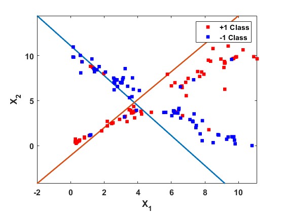
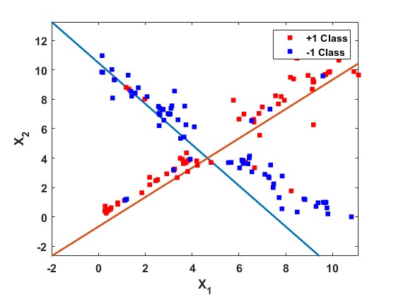
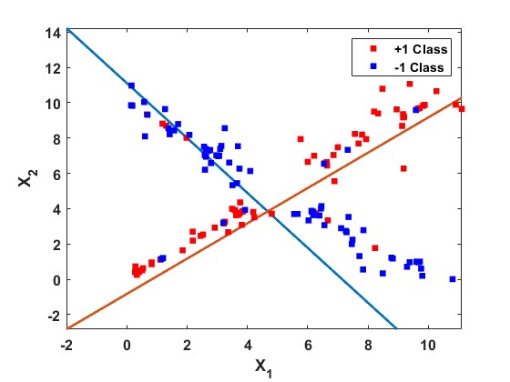
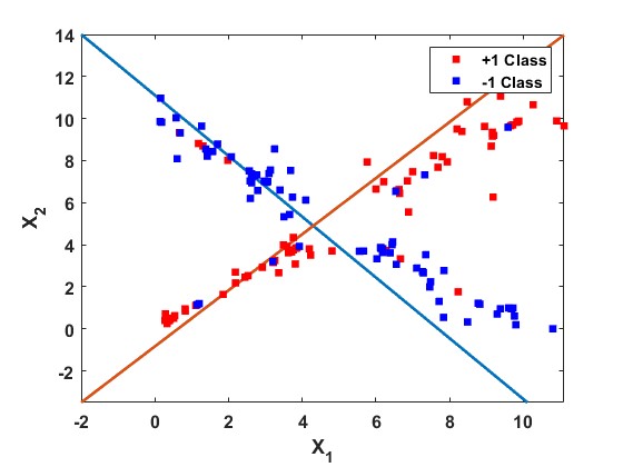
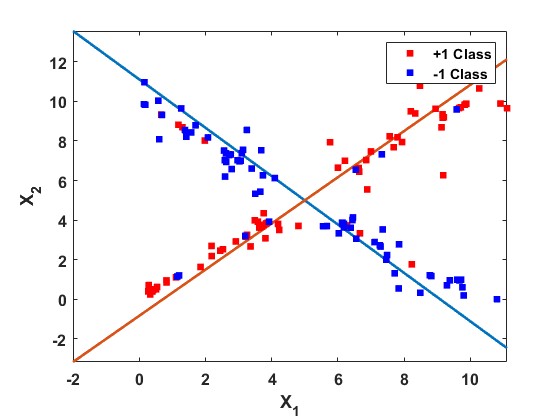
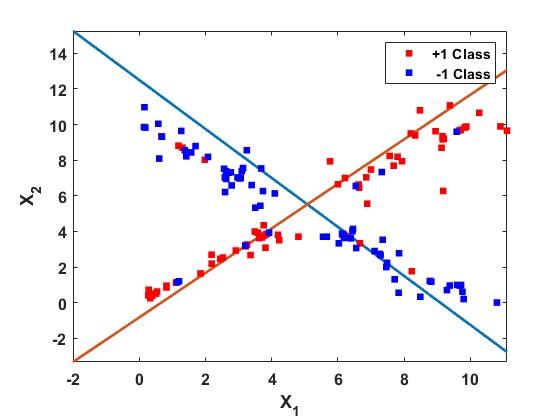
We first construct a two-class cross-plane dataset. Lines $X_{2}=X_{1}$ and $X_{2}=-X_{1}+10$ generate the training dataset for $+1$ and $-1$ classes, respectively. The values of $X_{1}$ is taken randomly within the range $[0,4]$ and $[6,10]$. There are $20$ samples in each of the two classes. We added $8$ outliers to Class $+1$ and $7$ outliers to Class $-1$ to evaluate the robustness. The test dataset is generated in a similar manner to the training data, with the inclusion of uniformly distributed random noise to both the variables $X_{1}$ and $X_{2}$. A total of $72$ samples in each of the two classes. We evaluate our proposed IF-GEPSVM and IF-IGEPSVM models along with the baseline models, to this training data. Fig. 1 visually represents the corresponding proximal planes, and Table 1 shows the ACC of the proposed model IF-GEPSVM and IF-IGEPSVM along with the baseline models. The proposed IF-GEPSVM and IF-IGEPSVM models secured the first and second positions with an ACC of $89.28\%$ and $86.04\%$, respectively. As a result, the proposed IF-GEPSVM and IF-IGEPSVM outperformed the baseline models.

Although Fig. 1 looks similar, there are the following major differences that can be observed by a reader: Figs. 1(a), 1(b), 1(c), and 1(d) illustrates that the models do not fit the line across the data points in the cross-place dataset correctly, causing the hyperplane to deviate and misclassify data points. This misalignment is particularly evident in the negative hyperplane, which is far from the negative class data points because some positive class data points are misclassified. These misclassified points are outliers, which deviate significantly from the rest of the data, and adversely affect the model’s performance. Therefore, the baseline Pin-GTSVM, GEPSVM, IGEPSVM, and CGFTSVM-ID models tend to yield biased results. However, as shown in Figs. 1(e) and 1(f), our proposed IF-GEPSVM and IF-IGEPSVM models demonstrate superior classification ability, even after introducing outliers. It utilizes an intuitionistic fuzzy membership scheme to mitigate the impact of noise and outliers, ensuring the hyperplane fits the data points correctly. This robustness to outliers is achieved through a membership and non-membership scheme, which enhances overall model performance. Our proposed models show that they can fit the hyperplane correctly and handle noisy datasets better. These results validate the practicality and feasibility of our IF-GEPSVM and IF-IGEPSVM proposed model, highlighting its improved classification capability in the presence of noise and outliers.

Table 1: Classification performance of proposed IF-GEPSVM and IF-IGEPSVM models and baseline models on the artificial dataset.
Model $\rightarrow$ Pin-GTSVM [41] GEPSVM [27] IGEPSVM [37] CGFTSVM-ID [23] IF-GEPSVM IF-IGEPSVM
Dataset \downarrow ACC𝐴𝐶𝐶ACC (%) ACC𝐴𝐶𝐶ACC(%) ACC𝐴𝐶𝐶ACC(%) ACC𝐴𝐶𝐶ACC (%) ACC𝐴𝐶𝐶ACC (%) ACC𝐴𝐶𝐶ACC (%)
$(c_{1},c_{2})$ $(\delta)$ $(\delta,\eta)$ $(c_{1},c_{2},r,\sigma)$ $(\delta)$ $(\delta,\eta)$
Crossplane 82.27 87 87 85.78 89.28 86.04
$(2^{-8},2^{-1})$ $(2^{-8})$ $(2^{-8},2^{-8})$ $(2^{-5},2^{-1},1,2^{2})$ $(2^{-8},2^{-8})$ $(2^{-8},2^{-8},2^{-8})$
represents the proposed models.
Boldface and underline depict the best and second-best models, respectively.
Refer to caption
(a)
Refer to caption
(b)
Refer to caption
(c)
Refer to caption
(d)
Refer to caption
(e)
Refer to caption
(f)
Figure 1: The learning outcome on the two-class cross-plane artificial data. Here, $X_{1}$ and $X_{2}$ represent the feature of the generated dataset.

6.3 Experiments on UCI and KEEL Datasets

In this subsection, we present an intricate analysis involving comparison of the proposed IF-GEPSVM and IF-IGEPSVM along with baseline Pin-GTSVM [41], GEPSVM [27], IGEPSVM [37] and CGFTSVM-ID models on $62$ benchmark UCI [7] and KEEL [6] datasets for the linear and non-linear cases. The classification ACC along with the optimal parameters of the proposed IF-GEPSVM and IF-IGEPSVM models against the baseline models are presented in Table 2. From the table, it is evident that the proposed IF-GEPSVM and IF-IGEPSVM models achieved the highest ACC on the majority of the datasets. The average ACC of the proposed IF-GEPSVM and IF-IGEPSVM models along with the baseline Pin-GTSVM, GEPSVM, IGEPSVM, and CGFTSVM-ID models are $78.20\%$ $81.00\%$, $70.44\%$, $72.33\%$, $74.02\%$ and $77.92\%$, respectively. In terms of average ACC, the proposed IF-IGEPSVM secured the top position, while the proposed IF-GEPSVM achieved the second top position. This observation strongly emphasizes the significant superiority of the proposed models compared to baseline models. As the average ACC can be influenced by exceptional performance in one dataset that compensates for losses across multiple datasets, it might be a biased measure. To mitigate this concern, it becomes essential to individually rank each model for each dataset, enabling a comprehensive assessment of their respective capabilities. In the ranking scheme [5], the model with the poorest performance on a dataset receives a higher rank, whereas the model achieving the best performance is assigned a lower rank. Assume that there are $q$ models being evaluated on a total of $N$ datasets. $r_{j}^{i}$ represents the rank of the $j^{th}$ model on the $i^{th}$ dataset. Then the average rank of the $j^{th}$ model is calculated as: $R_{j}=\frac{1}{N}\sum_{i=1}^{N}r_{j}^{i}$. The average ranks of the proposed IF-GEPSVM and IF-IGEPSVM models along with the baseline Pin-GTSVM, GEPSVM, IGEPSVM, and CGFTSVM-ID are $2.72$, $2.28$, $4.77$, $4.35$, $3.88$ and $3.01$, respectively. The proposed IF-GEPSVM and IF-IGEPSVM models achieved the lowest average range among the baseline models. Hence the proposed IF-GEPSVM and IF-IGEPSVM models emerged as the better generalization performance. Now we conduct the statistical tests to determine the significance of the results. Firstly, we employ the Friedman test [8] to determine whether the models have significant differences. Under the null hypothesis, it is presumed that all the models exhibit an equal average rank, signifying equal performance. Friedman statistics follow the chi-square ($\chi_{F}^{2}$) distribution with $(q-1)$ degree of freedom (d.o.f). The value of $\chi_{F}^{2}$ is calculated as: $\chi_{F}^{2}=\frac{12N}{q(q+1)}\left[\sum_{i=1}^{q}R_{j}^{2}-\frac{q(q+1)^{2}}{4}\right]$. The $F_{F}$ statistic follows an $F$-distribution [18] with d.o.f $(q-1)$ and $(N-1)(q-1)$, and is calculated as: $F_{F}=\frac{(N-1)\chi_{F}^{2}}{N(q-1)-\chi_{F}^{2}}$. For $N=62$ and $q=6$, we get $\chi_{F}^{2}=86.56$ and $F_{F}=23.63$. From the $F$-distribution table, $F_{F}(5,305)=2.2435$ at $5\%$ level of significance. Since $F_{F}=23.63>2.2435$, thus we reject the null hypothesis. As a result, there exists a statistical distinction among the models being compared. Now, we employ the Nemenyi post hoc test [5] to examine the pairwise distinctions between the models. The value of the critical difference $(C.D.)$ is evaluated as: $C.D.=q_{\alpha}\sqrt{\frac{q(q+1)}{6N}}$, where $q_{\alpha}$ is the critical value, $C.D.$ is critical difference for $q$ models using $N$ datasets. We get $C.D.=0.9576$ at $5\%$ level of significance. The average differences in ranking between the proposed IF-GEPSVM and IF-IGEPSVM models along with the baseline Pin-GTSVM, GEPSVM, IGEPSVM, and CGFTSVM-ID models are as follows: $(2.05,2.49)$, $(1.63,2.07)$, $(1.16,1.60)$, and $(0.29,0.73)$, respectively. As per the Nemenyi post hoc test, the proposed IF-GEPSVM and IF-IGEPSVM models show significant differences compared to the baseline models, except for CGFTSVM-ID. However, the proposed IF-GEPSVM and IF-IGEPSVM models outperform the CGFTSVM-ID model in terms of average rank. Taking into account all these findings, we can conclude that the proposed IF-GEPSVM and IF-IGEPSVM models demonstrate competitive performance compared to the baseline models.

Table 2: Classification performance of proposed IF-GEPSVM and IF-IGEPSVM models and baseline models on UCI and KEEL datasets with linear kernel.
Model $\rightarrow$ Pin-GTSVM [41] GEPSVM [27] IGEPSVM [37] CGFTSVM-ID [23] IF-GEPSVM IF-IGEPSVM
Dataset \downarrow ACC𝐴𝐶𝐶ACC (%) ACC𝐴𝐶𝐶ACC (%) ACC𝐴𝐶𝐶ACC (%) ACC𝐴𝐶𝐶ACC (%) ACC𝐴𝐶𝐶ACC (%) ACC𝐴𝐶𝐶ACC (%)
$(c_{1},c_{2})$ $(\delta)$ $(\delta,\eta)$ $(c_{1},c_{2},r,\sigma)$ $(\delta,\sigma)$ $(\delta,\eta,\sigma)$
acute_nephritis 79.86 78.89 74.44 100 80.56 88.89
$(120\times 6)$ $(2^{2},2^{-2})$ $(2)$ $(2^{-4},2^{-8})$ $(2^{-5},2^{-5},0.5,2^{3})$ $(2^{-4},2^{-8})$ $(2^{-7},2^{-8},2^{-8})$
adult 69.78 79.63 79.72 75.56 80.87 89.58
$(48842\times 14)$ $(2,2^{-4})$ $(2^{3})$ $(2^{-3},2^{-8})$ $(2^{-8},2^{-6},0.5,2^{4})$ $(2^{8},2^{-7})$ $(2^{-1},2^{-8},2^{-5})$
aus 78.28 88.41 88.41 89.66 88.89 88.41
$(690\times 15)$ $(2^{4},2^{6})$ $(2^{8})$ $(2^{-1},2^{-8})$ $(2^{2},2^{3},1,2^{2})$ $(2,2^{-8})$ $(2^{-4},2^{-8},2^{-8})$
bank 69.03 84.37 87.61 78.66 89.06 88.5
$(4521\times 16)$ $(2,2)$ $(2^{-8})$ $(2^{-5},2^{-8})$ $(2^{-5},2^{5},0.5,2^{1})$ $(2^{8},2^{-5})$ $(2^{-6},2^{-2})$
blood 53.88 65.63 77.23 65.63 65.8 78.57
$(748\times 4)$ $(2^{-1},1)$ $(2^{3})$ $(2^{-4},2^{-8})$ $(2^{3},2^{-1},1,2^{-2})$ $(2^{7},2^{-8})$ $(2^{-3},2^{-8},2^{-6})$
breast_cancer_wisc_diag 93.25 85.88 85.29 93.25 95.29 94.71
$(569\times 30)$ $(2^{-1},1)$ $(2^{5})$ $(2^{-3},2^{-8})$ $(2^{2},2^{3},0.5,2^{2})$ $(2^{2},2^{-3})$ $(2^{-4},2^{-8},2^{-6})$
breast_cancer_wisc_prog 81 67.8 76.44 75.12 79.66 86.44
$(198\times 33)$ $(2^{-5},2^{3})$ $(2^{6})$ $(2^{-5},2^{-8})$ $(2^{-1},1,0.5,2^{-5})$ $(2^{-3},2^{-4})$ $(2^{-4},2^{4},2^{-1})$
breast_cancer 49.75 64.71 65.88 70.83 68.24 84.12
$(286\times 9)$ $(2^{6},2^{3})$ $(2^{-8})$ $(2^{8},2^{-8})$ $(1,2^{4},0.75,2^{2})$ $(2^{-8},2^{-3})$ $(2^{-3},2^{-2})$
breast_cancer_wisc 97.67 87.61 98.09 98.86 98.09 98.09
$(699\times 9)$ $(1,2^{-1})$ $(2^{8})$ $(2,2^{-6})$ $(2^{5},2^{-5},1,2^{1})$ $(2^{7},2^{-8})$ $(2^{-2},2^{-8},2^{-8})$
brwisconsin 88.78 96.08 96.57 98.13 97.06 97.06
$(683\times 10)$ $(2^{4},1)$ $(2^{7})$ $(1,2^{-8})$ $(2^{2},2^{-5},0.625,2^{2})$ $(2^{7},2^{-5})$ $(2^{-2},2^{7},2^{-8},2^{-8})$
bupa or liver-disorders 58.56 59.22 62.14 67.99 78.93 78.93
$(345\times 7)$ $(2^{-3},2^{2})$ $(2^{6})$ $(2^{-8},2^{-8})$ $(2^{-5},2^{4},0.625,1)$ $(2^{-8},2^{-8})$ $(2^{-4},2^{-8})$
checkerboard_Data 87.89 88.41 88.41 89.66 88.89 88.41
$(690\times 15)$ $(2^{-6},2^{-4})$ $(2^{8})$ $(2^{-1},2^{-8})$ $(2^{2},2^{3},1,2^{2})$ $(2,2^{-8})$ $(2^{-4},2^{-8},2^{-8})$
chess_krvkp 91.31 66.91 71.09 86.12 76.72 74.43
$(3196\times 36)$ $(2^{5},2^{-1})$ $(2^{-2})$ $(2^{-2},2^{-8})$ $(2^{4},2^{-5},0.625,2^{-5})$ $(2^{3},2^{-3})$ $(2^{-2},2^{6},2^{-8})$
cmc 66.19 63.95 65.99 67.06 69.61 71.95
$(1473\times 10)$ $(1,1)$ $(2^{-8})$ $(2^{-3},2^{-8})$ $(1,2^{4},0.5,2^{2})$ $(2^{-8},2^{-8})$ $(2^{-8},2^{-8},2^{-8})$
conn_bench_sonar_mines_rocks 77.42 64.52 62.9 59.68 79.35 78.39
$(208\times 60)$ $(2^{2},2^{-4})$ $(2^{-1})$ $(2^{2},2^{-8})$ $(2^{5},2^{-5},0.5,2^{4})$ $(2^{6},2^{-4})$ $(2^{6},2^{-8},2^{-8},2^{-8})$
congressional_voting 58.63 53.08 52.31 63.27 71.54 75.38
$(435\times 16)$ $(2^{-2},2^{-7})$ $(2^{6})$ $(2^{-2},2^{-8})$ $(2^{1},2^{-5},0.875,2^{2})$ $(2^{7},2^{-8})$ $(2^{5},2^{-2},2^{-8})$
credit_approval 74.57 81.16 83.57 87.96 85.99 85.51
$(690\times 15)$ $(2^{-1},2^{3})$ $(2^{-8})$ $(2^{-3},2^{-8})$ $(2^{-5},2^{-4},1,2^{-7})$ $(2^{5},2^{-8})$ $(2^{-4},2^{5},2^{-8})$
crossplane130 100 86.82 97.89 100 100 100
$(130\times 3)$ $(2^{-1},2^{-4})$ $(2^{-8})$ $(2^{-8},2^{-8})$ $(2^{-5},2^{-5},0.5,2^{-5})$ $(2^{-8},2^{-7})$ $(2^{-8},2^{-8},2^{-5})$
crossplane150 78.26 95.72 96.78 100 100 100
$(150\times 3)$ $(2^{2},2^{-8})$ $(2^{-8})$ $(2^{-8},2^{-8})$ $(2^{-5},2^{-5},0.5,2^{-2})$ $(2^{-8},2^{-3})$ $(2^{-8},2^{-8},2^{-4})$
cylinder_bands 50.65 66.67 67.32 67.78 47.06 73.4
$(512\times 35)$ $(2^{-2},2^{-8})$ $(2^{-8})$ $(2^{2},2^{5})$ $(2^{-3},2^{2},0.875,2^{-5})$ $(2,2^{-3})$ $(2^{7},2^{-8},2^{-5})$
echocardiogram 90 89.74 89.74 81.21 94.87 94.87
$(131\times 10)$ $(2^{2},2^{7})$ $(2^{7})$ $(2^{-4},2^{-8})$ $(2^{5},2^{-1},0.875,1)$ $(1,2^{-8})$ $(2^{-4},2^{-8},2^{-8})$
fertility 74.07 50 46.67 66.67 80 80
$(100\times 9)$ $(2^{-4},2^{8})$ $(2^{-8})$ $(2^{6},2^{-8})$ $(2^{-1},2^{-2},1,2^{2})$ $(2^{8},2^{-3})$ $(2^{6},2^{-8},2^{-8},2^{-7})$
haber 59.72 63.74 65.93 64.32 83.63 84.73
$(306\times 4)$ $(2^{-5},2^{-2})$ $(2^{7})$ $(2^{-2},2^{-8})$ $(2^{-4},2^{3},0.75,2^{3})$ $(2^{2},2^{-8})$ $(2^{-8},2^{-8},2^{-4})$
haberman_survival 59.72 63.74 65.93 64.32 73.63 74.73
$(306\times 3)$ $(2^{-5},2^{-2})$ $(2^{-5})$ $(2^{-2},2^{-8})$ $(2^{-4},2^{3},0.75,2^{3})$ $(2^{2},2^{-8},2^{-8})$ $(2^{-8},2^{-8},2^{-8})$
heart_hungarian 73.69 80.68 84.09 80.83 86.36 86.36
$(294\times 12)$ $(2^{3},2^{2})$ $(2^{3})$ $(2^{-1},2^{-8})$ $(2^{5},2^{-1},0.875,2^{2})$ $(2,2^{-4})$ $(2,2^{4},2^{-3})$
horse_colic 74.84 74.55 76.36 82.93 80.91 82.73
$(368\times 25)$ $(2^{-2},1)$ $(2^{8})$ $(1,2^{-8})$ $(2^{3},2^{-2},1,2^{3})$ $(2^{4},2^{-5})$ $(2^{2},2^{4},2^{-8})$
ilpd_indian_liver 60.54 47.7 64.37 63.85 55.75 72.41
$(583\times 9)$ $(2^{-6},2)$ $(1)$ $(2^{-1},2^{-8})$ $(2^{2},2^{2},0.5,2^{8})$ $(2^{6},2^{-8})$ $(1,2^{-6},2^{-8})$
hepatitis 63.74 69.57 76.09 67.58 82.61 84.78
$(155\times 19)$ $(2^{-1},2^{-6})$ $(2^{6})$ $(2^{-4},2^{-8})$ $(2^{-3},2^{-1},0.625,2^{2})$ $(2^{4},2^{-6})$ $(2^{-1},2^{-8},2^{-7})$
hill_valley 54.78 59.23 56.2 88.43 60.14 58.73
$(1212\times 100)$ $(2,2^{7})$ $(1)$ $(2^{-6},2^{-8})$ $(2^{-3},2^{3},0.625,2^{2})$ $(2^{-7},2^{-8})$ $(2^{-8},2^{-8},2^{-8})$
iono 85.99 80 74.29 85.27 78.1 73.33
$(351\times 34)$ $(2^{-8},2^{-1})$ $(2^{2})$ $(2,2^{-8})$ $(2^{-4},2^{-3},0.75,2^{5})$ $(2^{-1},2^{-8})$ $(2^{4},2^{-8},2^{-8})$
ionosphere 85.46 81.9 74.29 86.78 78.1 90
$(351\times 33)$ $(2^{-2},2^{2})$ $(2)$ $(2^{-4},2^{-8})$ $(2^{-4},2^{-5},1,2^{2})$ $(2,2^{-8})$ $(2^{7},2^{-8},2^{-5})$
represents the proposed models.
Boldface and underline depict the best and second-best models, respectively.
Table 2: (Continued)
Model $\rightarrow$ Pin-GTSVM [41] GEPSVM [27] IGEPSVM [37] CGFTSVM-ID [23] IF-GEPSVM IF-IGEPSVM
Dataset \downarrow ACC𝐴𝐶𝐶ACC (%) ACC𝐴𝐶𝐶ACC (%) ACC𝐴𝐶𝐶ACC (%) ACC𝐴𝐶𝐶ACC (%) ACC𝐴𝐶𝐶ACC (%) ACC𝐴𝐶𝐶ACC (%)
$(c_{1},c_{2})$ $(\delta)$ $(\delta,\eta)$ $(c_{1},c_{2},r,\sigma)$ $(\delta,\sigma)$ $(\delta,\eta,\sigma)$
magic 65.78 74.71 74.17 74.89 76.31 72.51
$(19020\times 10)$ $(2^{-4},2^{3})$ $(2^{5})$ $(2^{-2},2^{-8})$ $(2^{-8},2^{-8},1,2^{4})$ $(2^{8},2^{-8})$ $(2^{-1},2^{-8},2^{-8})$
monks_1 69.27 76.75 56.75 72.51 66.27 84.34
$(556\times 6)$ $(2^{-2},2^{-1})$ $(2^{-8})$ $(2^{4},2^{-8})$ $(1,2^{-1},1,2^{2})$ $(2^{-8},2^{-8})$ $(2^{-6},2^{-8},2^{-8})$
monks_2 50 56.11 57.22 55.66 56.11 56.67
$(601\times 6)$ $(2^{-3},2^{-1})$ $(2^{6})$ $(2^{-5},2^{-8})$ $(2^{5},2^{2},0.625,2^{5})$ $(2^{6},2^{-4})$ $(2^{-8},2^{-8},2^{-4})$
monks_3 79.75 82.53 80.12 80.21 71.08 80.72
$(554\times 6)$ $(2,2^{6})$ $(2^{-8})$ $(2^{-5},2)$ $(2^{5},2^{2},0.875,2^{-5})$ $(2^{4},2^{-3})$ $(2,2^{-8},2^{-8})$
mammographic 64.02 70.49 81.6 83.16 82.99 80.9
$(961\times 5)$ $(2^{-8},1)$ $(2^{5})$ $(2^{4},2^{7})$ $(2^{5},2^{5},0.5,2^{-5})$ $(2^{2},2^{-3})$ $(2^{-1},2^{-8},2^{-5})$
molec_biol_promoter 57.48 54.84 51.61 76.92 41.94 71.94
$(106\times 57)$ $(2^{-4},2^{-4})$ $(2^{-6})$ $(2^{-1},2^{-8})$ $(2^{3},2^{-5},0.5,2^{5})$ $(2^{4},2^{-8})$ $(2^{-7},2^{-8},2^{-8})$
mushroom 65.45 97.62 96.8 95.85 97.50 92.89
$(8124\times 21)$ $(2^{-4},2^{-2})$ $(2)$ $(2^{-8},2^{-8})$ $(2^{-5},2^{-5},0.5,2^{7})$ $(2^{-8},2^{-8})$ $(2^{-5},2^{-8},2^{-8})$
oocytes_merluccius_nucleus_4d 68.3 70.92 68.3 82.84 71.9 79.67
$(1022\times 41)$ $(2,2^{-3})$ $(2^{7})$ $(2^{-2},2^{-8})$ $(2^{-4},2^{1},0.5,2^{5})$ $(2^{-7},2^{-7})$ $(2^{-2},2^{-8},2^{-7})$
oocytes_trisopterus_nucleus_2f 72.76 57.51 60.07 79.06 67.77 88.97
$(912\times 25)$ $(2^{7},2^{-5})$ $(2^{-1})$ $(2^{-1},2^{-8})$ $(2^{-3},2^{2},1,2^{4})$ $(2^{5},2^{-8})$ $(2^{-1},2^{3},2^{-8})$
musk_1 76.19 66.2 63.38 78.94 83.8 54.23
$(476\times 166)$ $(2^{-4},2^{5})$ $(2^{8})$ $(2^{-3},2^{4})$ $(1,2^{-1},1,2^{2})$ $(2^{3},2^{-8})$ $(2^{7},2^{-3},2^{-4})$
musk_2 81.65 87.01 84.03 80.53 94.78 95.46
$(6598\times 166)$ $(2^{-8},2^{-7})$ $(2^{8})$ $(2^{-4},2^{-8})$ $(2^{5},2^{2},0.625,2^{5})$ $(2^{6},2^{-7})$ $(2^{2},2^{-2},2^{-8})$
ozone 80.78 94.61 97.24 78.41 84.56 96.85
$(2536\times 72)$ $(2^{-1},2^{-4})$ $(2^{2})$ $(2^{-5},2^{-8})$ $(2^{-5},2^{4},0.5,2^{4})$ $(2^{-3},2^{-5})$ $(2^{-2},2^{-8},2^{-4})$
parkinsons 69.15 60.34 77.59 86.75 82.76 77.59
$(195\times 22)$ $(2,2^{-4})$ $(2^{6})$ $(2^{-8},2^{-8})$ $(2^{-3},2^{-5},0.625,2^{4})$ $(2^{-3},2^{-8})$ $(2^{-8},2^{-8},2^{-7})$
pima 50 76.09 77.83 73.21 76.09 83.91
$(768\times 8)$ $(2^{2},2^{-4})$ $(2^{5})$ $(2^{-4},2^{2})$ $(2^{-5},2^{-2},0.25,2^{-4})$ $(2^{3},2^{-4})$ $(2^{-3},2^{-8},2^{-7})$
pittsburg_bridges_T_OR_D 43.33 50 50 45 63.33 50
$(102\times 7)$ $(2^{2},2^{-4})$ $(2^{7})$ $(2,2^{-8})$ $(1,2^{-2},1,2^{2})$ $(1,2^{-8})$ $(2^{3},2^{-8},2^{-4})$
planning 44.44 64.81 68.52 40.28 55.56 61.11
$(182\times 12)$ $(2^{-8},2^{2})$ $(2^{-7})$ $(2^{-3},2^{-8})$ $(2^{-5},2^{-5},0.875,2^{3})$ $(2^{-4},2^{-3})$ $(2^{-4},2^{6},2^{-8})$
ringnorm 62.76 75.99 76.8 75.28 75.85 75.97
$(7400\times 20)$ $(2^{-2},2^{3})$ $(2^{8})$ $(2^{6},2^{-8})$ $(2^{-8},2^{-7},1,2^{7})$ $(2^{7},2^{-4})$ $(1,2^{-8},2^{-1})$
sonar 66.19 62.9 66.13 73.76 74.19 74.19
$(208\times 61)$ $(2^{-7},1)$ $(2^{5})$ $(2^{-7},2^{-8})$ $(2^{5},2^{3},0.875,2^{-5})$ $(2^{2},2^{-8})$ $(2^{-4},2^{-8},2^{-5})$
spambase 61.79 64.06 63.48 81.45 87.86 83.11
$(4601\times 57)$ $(2^{-3},2^{4})$ $(2^{-8})$ $(2^{-6},2^{-8})$ $(2^{-8},2^{-8},0.5,2^{8})$ $(2^{-2},2^{-8})$ $(2^{-3},2^{-8},2^{-8})$
statlog_australian_credit 50.79 55.07 62.8 58.63 55.07 64.25
$(690\times 14)$ $(2^{3},2^{-1})$ $(2^{8})$ $(1,2^{-8})$ $(2^{5},2^{-2},1,2^{2})$ $(2^{7},2^{-4})$ $(2^{-1},2^{-3},2^{-3})$
statlog_german_credit 68.51 72 70.33 77.42 80 79.67
$(1000\times 24)$ $(1,2^{-4})$ $(2^{3})$ $(2^{-2},2^{-8})$ $(2^{2},2^{1},1,2^{1})$ $(2^{5},2^{-3})$ $(2^{-3},2^{-8},2^{-3})$
spect 59.84 53.16 55.7 71.57 66.96 65.7
$(265\times 22)$ $(2^{-1},2^{7})$ $(2^{-1})$ $(2^{-4},2^{-8})$ $(2^{4},1,1,2^{3})$ $(2^{-4},2^{-3})$ $(2^{-8},2^{-8},2^{-8})$
spectf 81.09 66.25 75 85.06 72.5 80
$(267\times 44)$ $(2,2^{8})$ $(1)$ $(2^{-5},2^{6})$ $(2^{1},2^{-3},0.75,2^{4})$ $(2^{-5},2^{-8})$ $(2^{-5},2^{7},2^{-4})$
statlog_heart 81.44 83.95 83.95 86.08 81.48 81.48
$(270\times 13)$ $(2^{-3},2^{-3})$ $(1)$ $(2^{-1},2^{-8})$ $(2^{4},2^{-1},0.75,2^{-5})$ $(2^{2},2^{-6})$ $(2^{-8},2^{-8},2^{-8})$
titanic 50 78.03 78.03 70.51 77.27 74.24
$(2201\times 3)$ $(2^{-5},2^{-8})$ $(2^{7})$ $(2^{-2},2^{-8})$ $(2^{-5},2^{-3},0.625,2^{2})$ $(2^{6},2^{-4})$ $(2^{2},2^{-8},2^{-3})$
twonorm 82.87 87.79 87.7 85.75 97.9 98.05
$(7400\times 20)$ $(2^{-8},2^{-3})$ $(2^{7})$ $(2^{-7},2^{4})$ $(2^{-8},2^{-8},0.5,2^{6})$ $(2^{6},2^{-8})$ $(1,2^{-8},2^{-8})$
tic_tac_toe 76.81 71.43 73.52 96.81 97.91 97.91
$(958\times 9)$ $(2^{3},2)$ $(2^{-8})$ $(2^{-8},2^{-8})$ $(2^{-5},2^{-5},0.5,2^{-5})$ $(2^{-8},2^{-8})$ $(2^{-6},2^{4},2^{-3})$
vehicle1 70.13 75.49 76.28 81.18 77.87 77.87
$(846\times 19)$ $(2^{5},2^{7})$ $(2^{-6})$ $(2^{-6},2^{-8})$ $(2^{-1},1,0.5,2^{1})$ $(2^{-1},2^{-4})$ $(1,2^{-8},2^{-8})$
vertebral_column_2clases 68.82 70.97 67.74 76.27 76.34 73.41
$(310\times 6)$ $(2^{-8},2^{-8})$ $(2^{-8})$ $(2^{2},2^{-8})$ $(2^{-1},2^{5},0.75,2^{3})$ $(2^{4},2^{-3})$ $(2^{3},2^{7},2^{-4})$
vowel 90.87 78.18 80.2 91.06 89.86 92.57
$(988\times 11)$ $(2^{-8},2^{4})$ $(2^{2})$ $(2^{-7},2^{-8})$ $(2^{5},2^{1},0.75,2^{-5})$ $(2^{-3},2^{-4})$ $(2^{-8},2^{-8},2^{-8})$
wpbc 69.69 62.07 74.14 68.53 68.97 72.41
$(194\times 34)$ $(2^{-8},2^{4})$ $(2^{-6})$ $(2^{-5},2^{-8})$ $(2^{1},1,0.625,2^{-5})$ $(2^{-3},2^{-6})$ $(2^{-8},2^{-8},2^{-8})$
Average $ACC$ 70.44 72.33 74.02 77.92 78.20 81.00
Average Rank 4.77 4.35 3.88 3.01 2.72 2.28
represents the proposed models.
Boldface and underline depict the best and second-best models, respectively.
Table 3: Pairwise win-tie-loss test of proposed IF-GEPSVM and IF-IGEPSVM models along with baseline models on UCI and KEEL datasets with linear kernel.
Pin-GTSVM [41] GEPSVM [27] IGEPSVM [37] CGFTSVM-ID [23] IF-GEPSVM
GEPSVM [27] [37, 0, 25]
IGEPSVM [37] [39, 1, 22] [36, 6, 20]
CGFTSVM-ID [23] [50, 2, 10] [44, 1, 17] [39, 0, 23]
IF-GEPSVM [48, 1, 13] [47, 3, 12] [46, 1, 15] [33, 2, 27]
IF-IGEPSVM [57, 1, 4] [49, 3, 12] [45, 5, 12] [38, 2, 22] [30, 12, 20]
represents the proposed models.
Table 4: Classification performance of proposed IF-GEPSVM and IF-IGEPSVM models and baseline models on UCI and KEEL datasets with non-linear kernel.
Model $\rightarrow$ Pin-GTSVM [41] GEPSVM [27] IGEPSVM [37] CGFTSVM-ID [23] IF-GEPSVM IF-IGEPSVM
Dataset \downarrow ACC𝐴𝐶𝐶ACC (%) ACC𝐴𝐶𝐶ACC (%) ACC𝐴𝐶𝐶ACC (%) ACC𝐴𝐶𝐶ACC (%) ACC𝐴𝐶𝐶ACC (%) ACC𝐴𝐶𝐶ACC (%)
$(c_{1},c_{2},\sigma)$ $(\delta,\sigma)$ $(\delta,\eta,\sigma)$ $(c_{1},c_{2},r,\sigma)$ $(\delta,\sigma)$ $(\delta,\eta,\sigma)$
acute_nephritis 86.11 93.78 91.64 100 97 100
$(120\times 6)$ $(2^{-8},2^{-8},2^{-4})$ $(2,2^{-8})$ $(2^{-8},2^{-8},2^{-1})$ $(2^{-5},2^{-5},0.5,2^{-1})$ $(2^{-8},2^{-2})$ $(2^{-8},2^{-8},2^{-2})$
adult 76.67 78.65 75.45 80.48 84.46 86.65
$(48842\times 14)$ $(2^{-7},2^{-8},2^{2})$ $(2^{4},2^{7})$ $(2^{-4},2^{-5},2^{3})$ $(2^{-4},2^{-1},1,2^{-2})$ $(2^{-4},2^{-7})$ $(2^{-7},2^{-4},2^{-1})$
aus 85.02 85.99 88.38 85.2 87.21 88.38
$(690\times 15)$ $(2^{-6},2^{-5},2^{7})$ $(2^{4},2^{3})$ $(2^{-3},2^{-8},2^{7})$ $(2^{-3},2^{-4},0.625,2^{3})$ $(2,2^{2})$ $(2^{-3},2^{7},2^{-1})$
bank 72.65 77.89 88.35 70.94 90.81 88.42
$(4521\times 16)$ $(2^{-4},2^{3},2^{-4})$ $(2^{-6},2^{2})$ $(2^{-3},2^{-8},2^{2})$ $(2^{-1},2^{-5},1,2^{3})$ $(2^{5},2^{-3})$ $(1,2^{-8},2^{2})$
blood 59.28 57.59 77.68 53.6 78.57 78.57
$(748\times 4)$ $(2^{-6},2^{-1},2)$ $(2^{2},2^{-4})$ $(2^{-2},2^{-5},2^{-3})$ $(2^{-4},2^{2},0.625,2^{2})$ $(2^{-8},2^{4})$ $(1,2^{-8},2^{2})$
breast_cancer 54.35 68.24 72.94 70.89 72.94 72.94
$(286\times 9)$ $(2^{-8},2^{-8},2^{-8})$ $(2^{8},2^{3})$ $(1,2^{-8},2^{-8})$ $(2^{-5},2^{-5},0.5,2^{-1})$ $(2^{-2},2^{6})$ $(2^{-1},2^{-8},2^{6})$
breast_cancer_wisc_diag 94.43 75.88 94.71 90.08 74.12 93.53
$(569\times 30)$ $(2^{-1},2^{3},2^{6})$ $(2^{3},2^{-3})$ $(2^{-6},2^{-8},2^{7})$ $(1,2^{1},1,2^{3})$ $(1,2^{5})$ $(2^{-8},2^{-8},2^{7})$
breast_cancer_wisc_prog 64.22 69.49 86.44 64.83 71.19 83.05
$(198\times 33)$ $(2,2^{-8},2^{7})$ $(2^{2},1)$ $(2^{-1},2^{-6},2^{2})$ $(2^{-5},2^{3},0.875,2^{3})$ $(2^{-8},2^{-8})$ $(2^{-7},2^{-8},2)$
breast_cancer_wisc 95.24 88.52 88.56 98.05 92.6 98.09
$(699\times 9)$ $(2^{-3},2^{7},2^{3})$ $(2^{5},2^{8})$ $(2^{4},2^{-8},2^{3})$ $(2^{-5},2^{5},0.875,2^{4})$ $(2^{2},2^{2})$ $(2^{5},2^{-8},2^{3})$
brwisconsin 95.96 87.25 76.23 88.74 89.22 96.23
$(683\times 10)$ $(2^{-8},1,2^{-1})$ $(2^{4},2^{2})$ $(2^{2},2^{-8},2^{6})$ $(2^{-3},1,0.5,2^{3})$ $(2^{-1},2^{6})$ $(2^{2},2^{-8},2^{6})$
bupa or liver-disorders 66.31 67.96 60.58 66.85 68.93 74.58
$(345\times 7)$ $(2^{-4},2^{-4},2^{5})$ $(2^{-4},2^{3})$ $(2^{-3},2^{-8},2^{-2})$ $(2^{-5},2^{-1},1,2^{2})$ $(2^{-2},2^{-1})$ $(2^{-3},2^{-8},2^{-2})$
checkerboard_Data 87.21 82.61 88.38 90.2 84.06 88.38
$(690\times 15)$ $(2^{-6},2^{-5},2^{7})$ $(2^{6},1)$ $(2^{-3},2^{-8},2^{7})$ $(2^{-3},2^{-4},0.625,2^{3})$ $(2,2^{-2})$ $(2^{-3},2^{-8},2^{7})$
chess_krvkp 66.76 65.8 66.49 70.16 70.85 75.67
$(3196\times 36)$ $(2^{-3},2^{-8},2^{-4})$ $(2^{4},2^{-3})$ $(2^{-7},2^{-8},2^{3})$ $(2^{-5},2^{3},0.625,2^{3})$ $(2,2^{4})$ $(2^{-6},2^{-8},2^{5})$
cmc 67.03 63.23 57.61 63.83 69.61 74.61
$(1473\times 10)$ $(2^{-2},1,2^{5})$ $(2^{-2},2^{4})$ $(2^{2},2^{-8},2^{6})$ $(2^{5},2^{2},0.875,2^{4})$ $(2^{-2},2)$ $(2^{2},2^{-8},2^{6})$
conn_bench_sonar_mines_rocks 50.65 54.84 69.35 54.84 76.45 80.87
$(208\times 60)$ $(2^{-8},1,2^{8})$ $(2^{7},2^{-2})$ $(2^{3},2^{-8},2^{8})$ $(2^{1},2^{1},0.5,2^{5})$ $(2^{-5},2^{7})$ $(2^{3},2^{-4},2^{3})$
congressional_voting 53.66 60 64.62 62.35 63.08 57.69
$(435\times 16)$ $(2^{-4},2^{-3},2^{-2})$ $(2^{8},2^{-1})$ $(2^{-1},2^{-8},2^{2})$ $(2^{-3},2^{-4},1,2^{1})$ $(2^{-6},2^{6})$ $(2,2^{-8},2^{2})$
credit_approval 62.45 51.06 63.09 86.55 69.42 73.09
$(690\times 15)$ $(2^{4},2^{2},2^{4})$ $(2^{7},2^{-1})$ $(2^{5},2^{-8},2^{2})$ $(2^{4},1,0.75,2^{2})$ $(2^{-8},2^{8})$ $(2^{7},2^{-8},2^{2})$
crossplane130 92.87 91.65 93.65 95 95.89 95.89
$(130\times 3)$ $(2^{-6},2^{-3},2^{3})$ $(2^{-5},2^{-1})$ $(2^{-8},2^{-8},1)$ $(2^{-5},2^{-5},0.5,2^{-1})$ $(1,1)$ $(2^{-8},2^{-8},1)$
crossplane150 87.78 89.68 80.45 95.73 96.67 99.56
$(150\times 3)$ $(2^{-1},1,2^{-6})$ $(2,2^{6})$ $(2^{-8},2^{-8},1)$ $(2^{-5},2^{-5},0.5,2^{-3})$ $(2^{6},2)$ $(2^{-8},2^{-8},1)$
cylinder_bands 62.3 60.78 64.05 71.33 65.86 66.01
$(512\times 35)$ $(2^{-4},2^{-3},2^{3})$ $(2^{3},2^{-5})$ $(2^{-3},2^{-8},2^{2})$ $(2^{-4},1,0.5,2^{2})$ $(2^{-8},2^{-1})$ $(2^{3},2^{-8},1)$
echocardiogram 77.93 66.67 89.74 86.38 69.23 94.87
$(131\times 10)$ $(2^{-8},2^{2},2^{6})$ $(2^{3},2^{-2})$ $(2^{-2},2^{-8},2^{3})$ $(2^{-5},1,0.5,2^{5})$ $(2^{-3},2^{7})$ $(2^{-4},2^{-8},2^{2})$
fertility 60 66.67 76.83 50 90 86.67
$(100\times 9)$ $(2^{-8},2^{-8},1)$ $(2^{8},2)$ $(2^{-8},2^{-8},1)$ $(2^{-2},2^{-3},0.125,2^{-1})$ $(2^{-8},2^{-8})$ $(2^{-8},2^{-8},1)$
haber 53.36 71.43 74.77 58.63 78.57 74.77
$(306\times 4)$ $(2^{2},2,2^{8})$ $(2^{6},2^{-5})$ $(2^{-3},2^{-5},2)$ $(2^{4},2^{2},0.75,2^{1})$ $(2^{-3},2^{4})$ $(2^{-3},2^{-8},2)$
haberman_survival 53.36 70.33 75.82 58.63 70.33 76.92
$(306\times 3)$ $(2^{2},2,2^{8})$ $(2^{-7},2^{6})$ $(1,2^{-8},1)$ $(2^{4},2^{2},0.75,2^{1})$ $(2^{5},2^{4})$ $(2,2^{-8},2)$
heart_hungarian 81.79 77.27 84.09 83.57 89.77 85.23
$(294\times 12)$ $(2^{-2},1,2^{8})$ $(2^{7},2^{3})$ $(2^{3},2^{-8},2^{8})$ $(2^{5},2^{3},1,2^{5})$ $(2^{-8},2^{8})$ $(2^{8},2^{-8},2^{7})$
horse_colic 76.88 83.64 82.45 85.75 85.45 84.73
$(368\times 25)$ $(2^{-4},2^{-1},2^{8})$ $(2^{6},2^{3})$ $(2^{-3},2^{-8},2^{5})$ $(2^{-1},2^{4},0.625,2^{3})$ $(2^{-1},2^{5})$ $(2^{-2},2^{-8},2^{2})$
ilpd_indian_liver 58.49 70.69 71.84 69.88 75.86 72.41
$(583\times 9)$ $(2^{-3},1,2^{3})$ $(2^{-2},2^{3})$ $(2^{-2},2^{-8},2^{-3})$ $(2^{-5},2^{-3},0.75,2^{5})$ $(2^{-9},2^{-3})$ $(2^{-6},2^{-8},2^{2})$
hepatitis 67.58 63.04 82.61 83.88 76.09 82.61
$(155\times 19)$ $(2^{-8},2^{-5},2^{3})$ $(2,1)$ $(2^{-3},2^{-8},2^{7})$ $(2^{5},2^{2},0.875,2^{2})$ $(2^{3},2^{8})$ $(2^{-5},2^{-8},2^{2})$
represents the proposed model.
Boldface and underline depict the best and second-best models, respectively.
Table 4: (Continued)
Model $\rightarrow$ Pin-GTSVM [41] GEPSVM [27] IGEPSVM [37] CGFTSVM-ID [23] IF-GEPSVM IF-IGEPSVM
Dataset \downarrow ACC𝐴𝐶𝐶ACC (%) ACC𝐴𝐶𝐶ACC (%) ACC𝐴𝐶𝐶ACC (%) ACC𝐴𝐶𝐶ACC (%) ACC𝐴𝐶𝐶ACC (%) ACC𝐴𝐶𝐶ACC (%)
$(c_{1},c_{2},\sigma)$ $(\delta,\sigma)$ $(\delta,\eta,\sigma)$ $(c_{1},c_{2},r,\sigma)$ $(\delta,\sigma)$ $(\delta,\eta,\sigma)$
hill_valley 67.76 65.89 69.87 56.49 70.42 71.89
$(1212\times 100)$ $(2^{-8},2^{-8},2^{-4})$ $(2^{-8},2^{2})$ $(2^{4},2^{-7},2^{-4})$ $(2^{-4},2^{4},0.625,2^{-5})$ $(2^{-4},2^{-7})$ $(2^{-8},2^{-2},2^{4})$
iono 88.89 85.71 81.84 91.61 76.19 91.84
$(351\times 34)$ $(2^{3},2^{-7},2^{-7})$ $(2^{8},2^{-2})$ $(2^{-7},2^{-8},2^{5})$ $(2^{-5},2^{2},0.625,2^{1})$ $(2^{-4},2^{-7})$ $(2^{-7},2^{-8},2^{5})$
ionosphere 89.46 90.48 72.38 90.68 86.67 88.57
$(351\times 33)$ $(2^{-8},2^{-4},2^{5})$ $(2^{6},2)$ $(2^{-4},2^{-8},2^{4})$ $(2^{-7},2^{-1},0.5,1)$ $(2^{-8},2^{2})$ $(2^{-3},2^{-8},2^{3})$
magic 54.56 45.89 52.43 58 62.67 58.87
$(19020\times 10)$ $(2^{-8},2^{-6},2^{-4})$ $(2^{-4},2^{3})$ $(2^{-8},2^{3},2^{4})$ $(2^{-8},2^{-7},0.625,2^{-7})$ $(2^{-8},2^{2})$ $(2^{-8},2^{-8},2^{-2})$
monks_1 79.77 46.99 59.99 72.4 58.43 88.55
$(556\times 6)$ $(2^{-8},2,2^{7})$ $(2,2^{-8})$ $(2^{-5},2^{-8},2^{4})$ $(2^{-2},1,0.5,2^{4})$ $(2^{-8},2^{-1})$ $(2^{-8},2^{-8},2)$
monks_2 71.96 75.56 73.33 79.39 79.44 86.67
$(601\times 6)$ $(2^{-3},2,1)$ $(2^{-8},2^{-8})$ $(2^{-8},2,2^{6})$ $(2^{-4},2^{2},0.5,1)$ $(2^{-1},2^{-1})$ $(2^{-8},2^{-8},2^{2})$
monks_3 76.99 47.59 86.14 93.98 75.9 77.11
$(554\times 6)$ $(1,1,2^{2})$ $(2^{4},2^{-6})$ $(2^{-8},2^{-8},2)$ $(2^{-5},2^{2},1,2^{1})$ $(2,2)$ $(2^{-7},2^{-8},2)$
mammographic 68.03 75.35 82.64 82.05 71.88 82.29
$(961\times 5)$ $(2^{-7},2^{-8},2^{6})$ $(2^{-2},1)$ $(2^{-3},2^{-8},2^{8})$ $(2^{-1},2^{-2},0.625,2^{1})$ $(2^{8},2^{7})$ $(2^{-7},2^{-8},1)$
molec_biol_promoter 86.75 48.39 70.97 61.54 88.89 93.55
$(106\times 57)$ $(2^{-2},2^{-5},2^{6})$ $(2^{5},2^{7})$ $(2^{3},2^{-8},2^{7})$ $(2^{2},2^{1},0.5,2^{4})$ $(2^{-2},2^{5})$ $(2^{4},2^{-8},1)$
mushroom 65.64 65.67 68.79 70.49 71.82 75.65
$(8124\times 21)$ $(2^{-2},2^{3},2^{-4})$ $(2^{-5},2^{6})$ $(2^{8},2^{-5},2^{-4})$ $(2^{-8},2^{-8},0.5,2^{-5})$ $(2^{-4},2^{-7})$ $(2^{4},2^{-7},2^{-2})$
oocytes_merluccius_nucleus_4d 58.91 59.93 50.59 81.4 79.86 74.84
$(1022\times 41)$ $(2^{-1},2^{-3},2^{4})$ $(2^{-1},2^{-5})$ $(2^{-3},2^{-8},2^{-1})$ $(2^{-5},2^{1},0.75,2^{2})$ $(2^{8},2^{5})$ $(2^{-5},2^{-8},2^{5})$
oocytes_trisopterus_nucleus_2f 68.1 65.93 55.93 78.53 72.45 79.65
$(912\times 25)$ $(2^{5},2,2^{5})$ $(1,2^{3})$ $(2^{-6},2^{-8},2^{7})$ $(2^{-5},2^{4},0.875,2^{2})$ $(2^{2},1)$ $(2^{-3},2^{-8},2^{5})$
musk_1 69.2 64.54 60.56 89.36 74.15 67.18
$(476\times 166)$ $(2^{8},2^{-5},2^{-5})$ $(2^{-7},2^{-2})$ $(2^{5},2^{-8},2^{6})$ $(2^{-2},1,0.5,2^{4})$ $(2^{6},2^{5})$ $(2^{2},2^{-8},2^{-1})$
musk_2 84.67 82.32 79.8 85 85.67 89.94
$(6598\times 166)$ $(2^{8},2^{4},2^{3})$ $(2^{8},2^{4})$ $(2^{6},2^{-7},2^{-4})$ $(2^{-4},2^{2},0.5,1)$ $(2^{4},2^{7})$ $(2^{3},2^{-8},2^{-5})$
ozone 87.89 83.64 73.82 79.3 92.45 96.67
$(2536\times 72)$ $(2^{8},2^{-3},2^{-7})$ $(2^{2},2^{-8})$ $(2^{6},2^{-8},2^{2})$ $(2^{-8},2^{-8},0.5,2^{-5})$ $(2^{5},2^{-2})$ $(2^{-6},2^{-8},2^{-3})$
parkinsons 71.37 74.14 76.21 71.28 93.1 81.03
$(195\times 22)$ $(2^{7},2^{-4},2^{7})$ $(2^{8},2^{-1})$ $(2^{-1},2^{-8},2^{2})$ $(2^{3},2^{4},0.75,2^{4})$ $(2^{5},2^{2})$ $(2^{3},2^{-8},1)$
pima 68.45 68.26 76.52 73.81 69.57 73.74
$(768\times 8)$ $(2^{-4},2^{7},2^{3})$ $(2^{5},2^{-4})$ $(1,2^{-8},2^{2})$ $(2^{4},2^{-1},1,2^{1})$ $(2^{-7},2^{5})$ $(2^{-1},2^{-8},2^{2})$
pittsburg_bridges_T_OR_D 46.67 83.33 81.27 73.81 73.33 100
$(102\times 7)$ $(2^{-8},2^{-8},2^{5})$ $(2^{-1},2^{-6})$ $(2^{-5},2^{-8},2^{7})$ $(2^{2},2^{1},1,2^{1})$ $(2^{-1},2^{6})$ $(2^{-7},2^{-8},2^{3})$
planning 45.83 75.93 66.67 68.89 72.22 66.67
$(182\times 12)$ $(2^{-3},2^{-8},2^{6})$ $(2^{-8},2^{-8})$ $(2^{-4},2^{-8},2^{3})$ $(2^{-4},2^{1},1,2^{4})$ $(2^{-8},2^{-8})$ $(2^{-8},2^{-8},2^{-8})$
ringnorm 64.45 67.89 58.83 71.58 72.65 80.54
$(7400\times 20)$ $(2^{-8},2^{5},2^{2})$ $(2^{-2},2^{2})$ $(2^{-8},2^{-8},2^{-4})$ $(2^{-8},2^{-8},0.5,2^{-5})$ $(2^{-4},2^{-7})$ $(2^{3},2^{-6},2^{5})$
sonar 69.89 54.84 64.83 81.9 70.95 64.83
$(208\times 61)$ $(1,2^{5},2^{7})$ $(2^{3},1)$ $(2^{-3},2^{-8},2^{7})$ $(2^{-2},2^{-4},0.5,2^{2})$ $(2^{-2},2)$ $(2^{-3},2^{-8},2^{7})$
spambase 78.65 76.87 65.42 85.45 86.64 87.42
$(4601\times 57)$ $(2^{-6},2^{-2},2^{-7})$ $(2^{6},2^{8})$ $(2^{2},2^{-8},2^{-4})$ $(2^{-5},2^{-4},0.5,2^{-5})$ $(2^{5},2^{-3})$ $(2^{-6},2^{-3},2^{-2})$
statlog_australian_credit 45.14 68.12 69.57 58.33 68.12 74.05
$(690\times 14)$ $(2^{8},2^{-4},2^{8})$ $(2,2^{5})$ $(2^{-8},2^{-8},1)$ $(1,2^{-5},0.75,2^{1})$ $(2^{-8},2^{-8})$ $(2^{-3},2^{-8},2^{-1})$
statlog_german_credit 70.79 75 74.67 75.47 73.33 78.67
$(1000\times 24)$ $(2^{-8},2^{-5},2^{7})$ $(2^{7},2^{6})$ $(2,2^{-8},2^{4})$ $(2^{5},2^{2},1,2^{3})$ $(2^{7},2^{7})$ $(2^{-4},2^{-8},2^{6})$
spect 63.1 55.7 67.09 65.69 65.82 59.49
$(265\times 22)$ $(2^{-8},2^{-4},2^{4})$ $(2^{8},2^{5})$ $(2^{-2},2^{-8},2^{7})$ $(2^{-3},2^{-4},0.875,2^{2})$ $(2^{5},2^{4})$ $(1,2^{-8},2^{4})$
spectf 77.82 72.5 72.5 85.85 78.75 90
$(267\times 44)$ $(2^{-3},2^{-8},2^{-1})$ $(2^{-8},2^{-8})$ $(2^{-5},2^{-8},2^{-2})$ $(2^{-5},2^{-2},0.5,2^{5})$ $(2^{-8},2^{-8})$ $(2^{-2},2^{-8},1)$
statlog_heart 78.88 77.78 82.72 84.56 81.73 82.72
$(270\times 13)$ $(2^{6},2^{6},2^{4})$ $(2^{8},2^{8})$ $(1,2^{-8},2^{3})$ $(2^{-5},2^{-5},1,2^{2})$ $(2^{-8},2^{3})$ $(2^{-6},2^{-8},2^{2})$
titanic 52.69 48.46 68.03 70.18 76.36 81.63
$(2201\times 3)$ $(2^{-8},2^{-7},1)$ $(2^{-4},2^{-8})$ $(2^{-1},2^{-8},2^{2})$ $(2^{-1},1,0.5,2^{5})$ $(2,2^{-1})$ $(2^{6},2^{-6},2^{2})$
twonorm 65.57 69.85 59.63 75.78 76.85 79.89
$(7400\times 20)$ $(2^{-7},2^{4},2^{6})$ $(2^{-4},2^{6})$ $(2^{-6},2^{-4},2^{6})$ $(2^{-5},2^{3},0.5,2^{-4})$ $(2^{-7},2^{-2})$ $(2^{2},2^{-8},2^{-2})$
tic_tac_toe 66.81 62.37 67.91 98.94 72.47 78.87
$(958\times 9)$ $(2^{-1},1,2^{4})$ $(2^{8},2^{-4})$ $(2^{-7},2^{-8},2^{8})$ $(2^{-5},2^{1},0.75,2^{2})$ $(2^{6},2^{8})$ $(2^{-8},2^{-8},2^{-2})$
vehicle1 73.66 74.31 74.83 76.46 74.95 74.83
$(846\times 19)$ $(2^{-6},2^{3},2^{5})$ $(2^{-6},2^{8})$ $(2^{-8},2^{-8},2^{7})$ $(2^{-5},2^{-1},0.5,2^{-1})$ $(2^{-8},2^{-5})$ $(2^{-8},2^{-8},2^{7})$
vertebral_column_2clases 65.4 64.48 58.82 75.4 75.48 76.78
$(310\times 6)$ $(2^{6},2^{2},2^{4})$ $(2^{8},1)$ $(2^{3},2^{-8},2^{8})$ $(2^{-4},2^{4},0.875,2^{2})$ $(2^{-3},2^{4})$ $(2^{7},2^{-8},2^{5})$
vowel 93.20 91.27 93.20 97.82 95.27 99.82
$(988\times 11)$ $(2^{-3},2^{5},2^{4})$ $(2^{8},1)$ $(2^{-8},2^{-8},2^{4})$ $(2^{5},2^{2},0.75,2^{1})$ $(2^{-7},2^{2})$ $(2^{-8},2^{-8},2^{2})$
wpbc 62.87 74.14 60.37 61.01 75.86 70.37
$(194\times 34)$ $(1,2^{3},2^{8})$ $(2^{2},2^{-2})$ $(2^{-5},2^{-8},2^{-7})$ $(2^{-2},1,1,2^{3})$ $(2^{-8},2^{-7})$ $(2^{-5},2^{-8},2^{7})$
Average $ACC$ 70.81 70.64 73.63 76.37 77.98 81.53
Average Rank 4.65 4.69 3.94 3.13 2.69 1.9
represents the proposed model.
Boldface and underline depict the best and second-best models, respectively.

Furthermore, to analyze the models, we use pairwise win-tie-loss sign test [5]. As per the win-tie-loss sign test, the null hypothesis assumes that the two models are considered equivalent if each model wins approximately $N/2$ datasets out of the total $N$ datasets. At $5\%$ level of significance, the two models are considered significantly different if each model wins on approximately $\frac{N}{2}+1.96\frac{\sqrt{N}}{2}$ datasets. If there is an even occurrence of ties between any two models, the ties are distributed equally among them. However, if the number of ties is odd, one tie is ignored, and the remaining ties are distributed equally among the given models. For $N=62$, if one of the models’ wins is at least $38.716$ then there exists a significant difference between the models. Table 3 illustrates the comparative performance of the proposed IF-GEPSVM and IF-IGEPSVM models along with the baseline models, presenting their outcomes in terms of pairwise wins, ties, and losses using UCI and KEEL datasets. In Table 3, the entry $[x,y,z]$ indicates that the model mentioned in the row wins $x$ times, ties $y$ times, and loses $z$ times in comparison to the model mentioned in the respective column. Table 3 distinctly illustrates that the proposed IF-IGEPSVM model demonstrates significant superiority compared to the baseline. Moreover, the proposed IF-GEPSVM model attains statistically significant distinctions from CGFTSVM-ID. Showcasing a notable level of performance, the proposed IF-GEPSVM model outperforms in $33$ out of $62$ datasets. Consequently, the proposed IF-GEPSVM and IF-IGEPSVM models exhibit significant superiority over existing models.

Table 5: Pairwise win-tie-loss test of proposed IF-GEPSVM and IF-IGEPSVM models along with baseline models on UCI and KEEL datasets with non-linear kernel.
Pin-GTSVM [41] GEPSVM [27] IGEPSVM [37] CGFTSVM-ID [23] IF-GEPSVM
GEPSVM [27] [29, 0, 33]
IGEPSVM [37] [37, 1, 24] [38, 1, 23]
CGFTSVM-ID [23] [50, 0, 12] [45, 1, 16] [40, 0, 22]
IF-GEPSVM [53, 0, 9] [53, 2, 7] [43, 1, 18] [37, 0, 25]
IF-IGEPSVM [57, 0, 5] [58, 0, 4] [46, 9, 7] [44, 1, 17] [43, 3, 16]
represents the proposed model.

For the non-linear case, the ACC values are shown in Table 4 for the proposed IF-GEPSVM and IF-IGEPSVM along with the baseline models. From Table 4, it is evident that IF-GEPSVM and IF-IGEPSVM demonstrate superior generalization performance in most of the datasets. It is clear that the proposed IF-IGEPSVM and IF-GEPSVM secure the first and second position with an average ACC of $81.53\%$ and $77.98\%$, and the baseline models i.e., Pin-GTSVM, GEPSVM, IGEPSVM and CGFTSVM-ID has the average ACC of $70.81\%$, $70.64\%$, $73.63\%$, and $76.37\%$, respectively. The average ranks of all the models based on ACC values are shown in Table 4. It can be noted that among all the models, our proposed IF-GEPSVM and IF-IGEPSVM hold the lowest average rank. The minimum rank of the model implies the better performance of the model. Furthermore, we conduct the Friedman test. For $N=62$ and $q=6$, we get $\chi_{F}^{2}=111.34$ and $F_{F}=34.188$. Since $F_{F}=34.188>2.2435$, the null hypothesis is rejected, indicating a statistical distinction difference between the models. Next, the Nemenyi post hoc test is used to compare the models pairwise. At $5\%$ level of significance, the value of $C.D.=0.9576$. The average rank differences between the proposed IF-GEPSVM and IF-IGEPSVM models with the baseline Pin-GTSVM, GEPSVM, IGEPSVM, and CGFTSVM-ID models are $(1.96,2.75)$, $(2,2.79)$, $(1.25,2.04)$, and $(0.44,1.23)$, respectively. As per the Nemenyi post hoc test, the proposed IF-GEPSVM and IF-IGEPSVM models exhibit significant differences compared to the baseline models, except for IF-GEPSVM with CGFTSVM-ID. However, the proposed IF-GEPSVM model surpasses the CGFTSVM-ID model in terms of average rank. Therefore, the proposed IF-GEPSVM and IF-IGEPSVM models demonstrated superior performance compared to the baseline models. We also perform a win-tie-loss sign test for the non-linear case. Table 5 illustrates the pairwise win-tie-loss outcomes of the compared models on UCI and KEEL datasets. In our case, if either of the two models emerges victorious in at least $38.716$ datasets, they are considered statistically distinct. Table 5 clearly illustrates that the proposed IF-GEPSVM and IF-IGEPSVM models exhibit statistically superior performance compared to the baseline Pin-GTSVM, GEPSVM, IGEPSVM, and CGFTSVM-ID models. Overall, from the preceding analysis, it is evident that the proposed IF-GEPSVM and IF-IGEPSVM models showcase competitive or even superior performance compared to the baseline models.

Table 6: Performance comparison of the proposed IF-GEPSVM and IF-IGEPSVM models against the baseline models on UCI and KEEL datasets with label noise.
Model $\rightarrow$ Noise Pin-GTSVM [41] GEPSVM [27] IGEPSVM [37] CGFTSVM-ID [23] IF-GEPSVM IF-IGEPSVM
Dataset \downarrow ACC𝐴𝐶𝐶ACC (%) ACC𝐴𝐶𝐶ACC (%) ACC𝐴𝐶𝐶ACC (%) ACC𝐴𝐶𝐶ACC (%) ACC𝐴𝐶𝐶ACC (%) ACC𝐴𝐶𝐶ACC (%)
$(c_{1},c_{2})$ $(\delta)$ $(\delta,\eta)$ $(c_{1},c_{2},r,\sigma)$ $(\delta,\sigma)$ $(\delta,\eta,\sigma)$
acute_nephritis $5\%$ 100 97.22 95.65 97.83 100 100
$(2^{-5},2^{-5})$ $(2^{4})$ $(2^{-8},2^{-8})$ $(2^{-5},2^{-3},0.5,2^{-5})$ $(2^{1},2^{-8})$ $(2^{-8},2^{-1},2^{-8})$
$10\%$ 97.83 63.89 90.85 91.3 100 100
$(2^{1},2^{-5})$ $(2^{4})$ $(2^{-8},2^{-8})$ $(2^{-5},2^{-4},0.75,2^{-5})$ $(2^{4},2^{-7})$ $(2^{-8},2^{4},2^{-5})$
$15\%$ 87.96 94.44 90.79 89.13 94.44 100
$(1,2^{6})$ $(2^{4})$ $(2^{-8},2^{-8})$ $(2^{2},2^{-5},0.5,2^{-5})$ $(2^{6},2^{-8})$ $(2^{-8},2^{4},2^{-8})$
$20\%$ 85.28 97.22 89.45 93.48 100 83.33
$(2^{5},2^{-5})$ $(2^{6})$ $(2^{-8},2^{-8})$ $(2^{3},2^{-4},0.5,2^{3})$ $(2^{-1},2^{-6})$ $(2^{-8},2^{-4},2^{-7})$
Average ACC 92.77 88.19 91.69 92.93 98.61 95.83
aus $5\%$ 87.56 87.44 77.29 86.08 88.41 88.41
$(2^{1},2^{-5})$ $(2^{8})$ $(2^{-8},2^{-8})$ $(2^{-5},2^{-2},0.75,2^{3})$ $(2^{4},2^{-8})$ $(2^{3},2^{6},2^{-8})$
$10\%$ 85.07 84.06 76.81 86.34 88.41 88.41
$(2^{-5},2^{-2})$ $(2^{8})$ $(2^{-8},2^{-8})$ $(2^{5},2^{2},1,1)$ $(2^{2},2^{-5})$ $(2^{-8},2^{2},2^{-5})$
$15\%$ 85.02 85.99 81.16 86.88 88.41 88.41
$(2^{-1},2^{-3})$ $(2^{8})$ $(2^{-8},2^{-8})$ $(2^{4},2^{-5},1,2^{-1})$ $(2^{2},2^{-7})$ $(2^{-7},2^{2},2^{-8})$
$20\%$ 88.54 85.02 73.43 84.25 89.37 80.19
$(2^{5},2^{-5})$ $(2^{8})$ $(2^{-8},2^{-8})$ $(2^{5},2^{-1},0.75,2^{4})$ $(2^{2},2^{-6})$ $(2^{-8},2^{3},2^{-1})$
Average ACC 86.55 85.63 77.17 85.89 88.65 86.35
breast_cancer_wisc_prog $5\%$ 68.87 59.32 76.27 71.81 81.36 84.75
$(2^{-5},2^{-4})$ $(2^{5})$ $(2^{-8},2^{-8})$ $(2^{-3},2^{-1},0.75,2^{3})$ $(2^{4},2^{-6})$ $(2^{-8},2^{2},2^{-6})$
$10\%$ 66.91 55.93 77.97 68.87 81.36 86.44
$(2^{-3},2^{-3})$ $(2^{4})$ $(2^{-8},2^{-8})$ $(2^{-1},2^{-2},0.75,2^{4})$ $(2^{4},2^{-5})$ $(2^{-5},2^{-1},2^{-6})$
$15\%$ 57.6 57.63 71.19 57.35 72.88 86.44
$(2^{2},2^{3})$ $(2^{2})$ $(2^{-7},2^{-8})$ $(1,2^{-5},0.875,2^{4})$ $(2^{4},2^{-6})$ $(2^{-3},2^{1},2^{-7})$
$20\%$ 46.69 59.32 74.58 45.59 74.58 71.19
$(2^{7},2^{7})$ $(2^{4})$ $(2^{-7},2^{-8})$ $(2^{4},2^{1},0.875,2^{4})$ $(2^{4},2^{-8})$ $(2^{-8},2^{6},2^{-8})$
Average ACC 60.02 58.05 75 60.91 77.54 82.2
credit_approval $5\%$ 81.16 83.57 86.47 86.95 86.47 85.51
$(2^{-5},2^{-3})$ $(2^{-4})$ $(2^{-8},2^{-8})$ $(2^{-2},2^{3},0.5,2^{1})$ $(2^{2},2^{-7})$ $(2^{-8},2^{2},2^{-7})$
$10\%$ 76.17 82.13 86.47 86.95 85.99 85.51
$(2^{-1},2^{-5})$ $(2^{-7})$ $(2^{-8},2^{-8})$ $(1,2^{-5},0.5,2^{-5})$ $(2^{2},2^{-6})$ $(2^{-8},2^{2},2^{-3})$
$15\%$ 56.92 77.78 85.99 86.95 85.51 85.51
$(2^{-5},2^{-3})$ $(2^{-1})$ $(2^{-8},2^{-8})$ $(2^{1},2^{-5},0.5,2^{1})$ $(2^{2},2^{-5})$ $(2^{-8},2^{4},2^{-6})$
$20\%$ 85.73 77.29 81.64 86.95 85.51 85.51
$(1,2^{-7})$ $(2^{-7})$ $(2^{-8},2^{-8})$ $(2^{2},2^{-2},0.75,2^{-5})$ $(2^{2},2^{-3})$ $(2^{-8},2^{4},2^{-8})$
Average ACC 75 80.19 85.14 86.95 85.87 85.51
vehicle1 $5\%$ 63.45 67.98 74.31 75.36 78.66 76.68
$(2^{-4},2^{-7})$ $(2^{-5})$ $(2^{-8},2^{-8})$ $(2^{3},2^{3},0.625,2^{1})$ $(2^{2},2^{-8})$ $(2^{-8},2^{4},2^{-2})$
$10\%$ 65.17 65.61 79.45 76.43 77.08 75.89
$(2^{-3},2^{-1})$ $(2^{-7})$ $(2^{-8},2^{-8})$ $(2^{1},1,0.875,2^{5})$ $(2^{6},2^{-8})$ $(2^{-2},2^{-4},2^{-8})$
$15\%$ 63.36 57.31 73.91 75.21 72.33 75.89
$(2^{-8},2^{-2})$ $(2^{-5})$ $(2^{-8},2^{-8})$ $(2^{3},2^{1},0.75,2^{5})$ $(2^{3},2^{-7})$ $(2^{-8},2^{-4},2^{-8})$
$20\%$ 64.87 53.75 75.49 79.27 73.91 75.49
$(2^{-3},2^{2})$ $(2^{-5})$ $(2^{-8},2^{-8})$ $(1,2^{-1},0.75,2^{3})$ $(2^{4},2^{2})$ $(2^{-7},2^{1},2^{-1})$
Average ACC 64.21 61.17 75.79 76.57 75.49 75.99
wpbc $5\%$ 67.52 70.69 75.86 67.36 74.14 74.14
$(2^{-4},2^{2})$ $(2^{-4})$ $(2^{-8},2^{-8})$ $(2^{2},1,0.5,2^{4})$ $(2^{4},2^{-8})$ $(2^{-8},2^{2},2^{-8})$
$10\%$ 52.17 65.52 70.69 63.02 62.07 74.14
$(2^{4},2^{5})$ $(2^{2})$ $(2^{-8},2^{-8})$ $(2^{2},2^{1},0.75,2^{4})$ $(2^{6},2^{-8})$ $(2^{-8},2^{1},2^{-6})$
$15\%$ 82.02 65.52 65.52 59.53 65.52 74.14
$(2^{-3},2^{4})$ $(2^{-4})$ $(2^{-8},2^{-8})$ $(2^{1},2^{-5},0.875,2^{3})$ $(2^{8},2^{-4})$ $(2^{-6},2^{1},2^{-4})$
$20\%$ 50.23 60.34 72.41 66.2 62.07 75.86
$(2^{6},2^{6})$ $(2^{-7})$ $(1,2^{-8})$ $(1,2^{-2},0.625,2^{2})$ $(2^{6},2^{-8})$ $(2^{-8},2^{6},2^{-7})$
Average ACC 62.98 65.52 71.12 64.03 65.95 74.57
Overall Average ACC 73.59 73.13 79.32 77.88 82.02 83.41
represents the proposed model.
Boldface and underline depict the best and second-best models, respectively.

6.4 Evaluation on UCI and KEEL Datasets with Added Label Noise

The evaluation conducted using UCI and KEEL datasets mirrors real-world scenarios. However, it’s important to recognize that data impurities or noise may arise from various factors. To demonstrate the efficacy of the proposed IF-GEPSVM and IF-IGEPSVM models, particularly in challenging conditions, we intentionally introduced label noise to specific datasets. We chose $6$ datasets to test the robustness of the models namely acute_nephritis, aus, breast_cancer_wisc_prog, credit_approval, vehicle1 and wpbc. To ensure fairness in model evaluation, we deliberately chose three datasets where the proposed IF-GEPSVM model did not attain the highest performance and three datasets where they achieved comparable results to an existing model with different levels of label noise. For a comprehensive analysis, we introduced label noise at different levels, including $5\%$, $10\%$, $15\%$, and $20\%$ to intentionally corrupt the labels of these datasets. Table 6 presents the ACC of all models for the selected datasets with $5\%$, $10\%$, $15\%$, and $20\%$ noise. Consistently, the proposed IF-GEPSVM and IF-IGEPSVM models exhibit superior performance over baseline models, demonstrating higher ACC. Significantly, they sustain this leading performance despite the presence of noise. The average ACC of the proposed IF-GEPSVM and IF-IGEPSVM on the acute_nephritis dataset at various noise levels are $98.61\%$ and $95.83\%$, respectively, surpassing the performance of the baseline models. On the aus dataset, both proposed models’ ACC are lower than the CGFTSVM-ID at $0\%$ noise level (refer to Table 2). However, the average ACC of the proposed models at different noise levels are $88.65\%$ and $86.35\%$, respectively, outperforming all the baseline models. On the credit_approval and vehicle1 datasets, the proposed models did not secure the top positions at $0\%$ noise level. However, with distinct noise levels, the proposed IF-GEPSVM and IF-IGEPSVM secured the second and third positions, respectively, on the credit_approval and vehicle1 datasets. On different levels of noise, the proposed IF-GEPSVM and IF-IGEPSVM models, with an average ACC of $65.95\%$, and $74.57\%$, surpass all the baseline models on wpbc dataset. At each noise level, IF-GEPSVM and IF-IGEPSVM emerge as the top performers, with overall average ACC of $82.02\%$ and $83.41\%$, respectively. By subjecting the model to rigorous conditions, we aim to demonstrate the exceptional performance and superiority of the proposed IF-GEPSVM and IF-IGEPSVM models, particularly in unfavorable scenarios. The above findings emphasize the importance of the proposed IF-GEPSVM and IF-IGEPSVM models as resilient solutions, capable of performing well in demanding conditions marked by noise and impurities.

6.5 Sensitivity Analysis

In this subsection, we perform sensitivity analyses on the hyperparameters $\delta$ and $\sigma$. Additionally, we investigate the impact of varying levels of label noise on the model.

Refer to caption
(a)
Refer to caption
(b)
Refer to caption
(c)
Refer to caption
(d)
Refer to caption
(e)
Refer to caption
(f)
Figure 2: Effect of parameters $\delta$ and $\sigma$ on the performance of the proposed IF-GEPSVM and IF-IGEPSVM models.

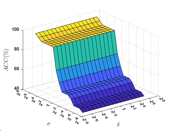
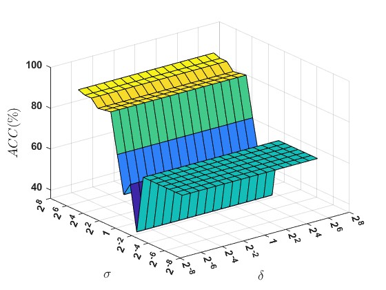
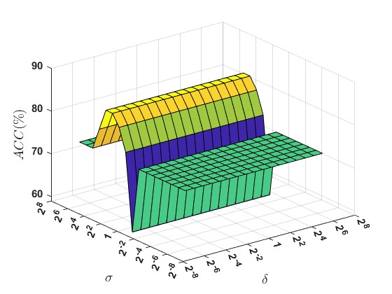
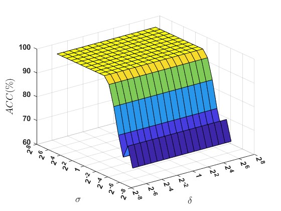
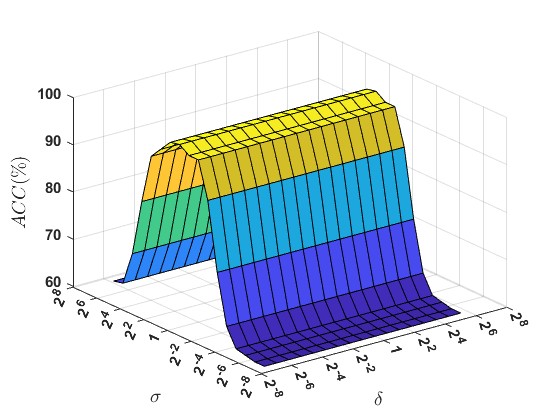
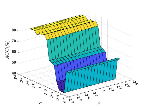
6.5.1 Sensitivity Analysis of Hyperparameter $\delta$ and $\sigma$

We assess the performance of the proposed IF-GEPSVM and IF-IGEPSVM models by adjusting the values of $\delta$ and $\sigma$. This comprehensive examination allows us to identify the configuration that optimizes predictive ACC and enhances the model’s robustness against unseen data. Fig. 2 depicts noticeable variations in the model’s ACC across different combinations of $\delta$ and $\sigma$ values, highlighting the sensitivity of our model’s performance to these particular hyperparameters. Based on the results depicted in Figs. 2(a) and 2(d), we observe the optimal performance of the proposed IF-GEPSVM and IF-IGEPSVM models within the $\sigma$ ranges of $2^{4}$ to $2^{8}$ and $2^{2}$ to $2^{8}$. Figs. 2(b) and 2(e) demonstrates an increase in testing ACC of the proposed IF-GEPSVM and IF-IGEPSVM models within the $\sigma$ range spanning from $2^{2}$ to $2^{8}$ and $2^{-2}$ to $2^{2}$. Similarly, in Figs. 2(c) and 2(f), the testing ACC within the ranges $1$ to $2^{7}$ and $2^{2}$ to $2^{8}$ of both the proposed IF-GEPSVM and IF-IGEPSVM models. These results suggest that, when considering the parameters $\sigma$ and $\delta$, the performance of both the proposed IF-GEPSVM and IF-IGEPSVM models is predominantly influenced by $\sigma$ rather than $\delta$. This highlights the importance of the kernel space and the effective extraction of non-linear features in the proposed IF-GEPSVM and IF-IGEPSVM models. Therefore, it is advisable to carefully consider the selection of the hyperparameter $\sigma$ in IF-GEPSVM and IF-IGEPSVM models to achieve superior generalization performance.

Refer to caption
(a)
Refer to caption
(b)
Refer to caption
(c)
Refer to caption
(d)
Figure 3: Effect of different labels of noise on the performance of the proposed IF-GEPSVM and IF-IGEPSVM models.

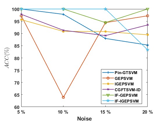
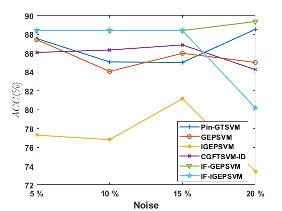
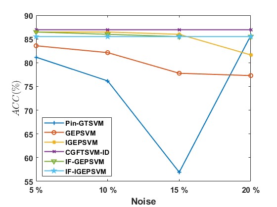
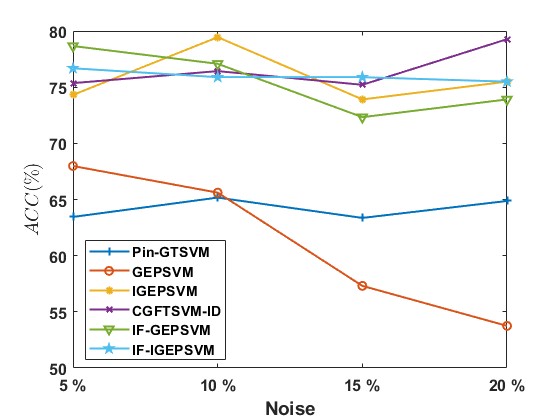
6.5.2 Sensitivity Analysis of Label Noise

The proposed IF-GEPSVM and IF-IGEPSVM models are designed with a primary focus on mitigating the adverse impact of noise. Their robustness is evidenced by their performance across different levels of label noise. The testing ACC of both the proposed IF-GEPSVM and IF-IGEPSVM models and the baseline models under varying levels of label noise is illustrated in Fig. 3. The performance is shown for the acute_nephritis, aus, credit_approval, and vehicle1 datasets. The performance of baseline models exhibits notable fluctuations, diminishing notably with varying levels of noise labels. In contrast, the proposed IF-GEPSVM and IF-IGEPSVM models consistently maintain superior performance across different noise levels.

Refer to caption
Figure 4: A visual representation of USPS database.
Table 7: Classification performance of proposed IF-GEPSVM and IF-IGEPSVM models and baseline models on USPS recognition datasets.
Model $\rightarrow$ Pin-GTSVM [41] GEPSVM [27] IGEPSVM [37] CGFTSVM-ID [23] IF-GEPSVM IF-IGEPSVM
Dataset \downarrow ACC𝐴𝐶𝐶ACC (%) ACC𝐴𝐶𝐶ACC (%) ACC𝐴𝐶𝐶ACC (%) ACC𝐴𝐶𝐶ACC (%) ACC𝐴𝐶𝐶ACC (%) ACC𝐴𝐶𝐶ACC (%)
$(c_{1},c_{2})$ $(\delta)$ $(\delta,\eta)$ $(c_{1},c_{2},r,\sigma)$ $(\delta)$ $(\delta,\eta)$
0 vs. 1 88.65 53.78 88.35 85.87 99.53 98.84
$(2^{-7},2^{-8})$ $(2^{5})$ $(2^{-6},2^{-8})$ $(2^{5},2^{-3},1,2^{-5})$ $(2^{-4})$ $(2^{-7},2^{-8})$
1 vs. 2 89.34 42.49 98.18 95.69 99.09 98.57
$(2^{-8},2^{-5})$ $(2^{-1})$ $(2^{-5},2^{-8})$ $(2^{3},2^{-3},0.875,2^{-5})$ $(2^{-7})$ $(2^{-8},2^{-8})$
2 vs. 3 87.5 95.24 92.19 95.5 96.38 88.51
$(2^{-8},2^{-4})$ $(2^{4})$ $(2^{-5},2^{-8})$ $(1,2^{-4},0.5,2^{-5})$ $(2^{2})$ $(2^{-5},2^{-8})$
3 vs. 4 89.38 91.04 89.84 96.23 98.01 94.46
$(2^{-8},2^{-8})$ $(2^{8})$ $(2^{-4},2^{-8})$ $(2^{5},2^{-5},0.5,2^{5})$ $(2^{4})$ $(2^{-5},2^{-8})$
5 vs. 6 80.96 92.04 94.84 90.27 92.47 93.82
$(2^{-7},2^{-8})$ $(2^{7})$ $(2^{-6},2^{-8})$ $(2^{5},2^{-5},0.5,2^{5})$ $(2^{4})$ $(2^{-7},2^{-8})$
2 vs. 7 92.25 97.67 92.64 97.54 98.26 96.1
$(2^{-5},2^{-6})$ $(2^{4})$ $(2^{-5},2^{-8})$ $(2^{5},2^{-4},0.5,2^{4})$ $(2^{1})$ $(2^{-6},2^{-8})$
3 vs. 8 88.75 85.19 88.67 87.29 87.8 88.90
$(2^{-8},2^{-2})$ $(2^{8})$ $(2^{-4},2^{-8})$ $(2^{5},2^{-2},0.5,2^{5})$ $(2^{6})$ $(2^{-4},2^{-8})$
2 vs. 5 91.99 91.08 91.08 90.22 92.09 87.92
$(2^{-8},2^{-3})$ $(2^{4})$ $(2^{-4},2^{-8})$ $(2^{5},2^{1},0.75,2^{4})$ $(2^{6})$ $(2^{-3},2^{-8})$
Average ACC 88.60 81.07 91.97 92.33 95.45 93.39
represents the proposed model.
Boldface and underline depict the best and second-best models, respectively.

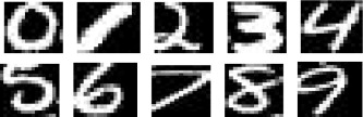
6.6 USPS recognition

The collection of grayscale images of handwritten digits ranging from 00 to $9$ can be found in the USPS database, accessible at https://cs.nyu.edu/~roweis/data.html. This is depicted in Fig. 4. There are a total of $1100$ images for each digit in the dataset, and each image has a size of $16\times 16$ pixels with $256$ different shades of gray (resulting in $1100$ examples per class with $256$ dimensions). In this case, we have chosen eight pairs of digits with varying levels of difficulty for classifying odd and even digits. The specific classes that have been selected can be found in Table 7. We use linear kernel to evaluate the experiment. The ACC of each model for classification is evaluated using the $10$-fold cross-validation. The performance of the proposed IF-GEPSVM and IF-IGEPSVM models along with the baseline models are presented in Table 7. Notably, IF-GEPSVM and IF-IGEPSVM models attained the first and second positions with average ACC of $95.45\%$ and $93.39\%$, respectively. In contrast, the baseline models, comprising Pin-GTSVM, GEPSVM, IGEPSVM, and CGFTSVM-ID, exhibited lower average ACC of $88.60\%$, $81.07\%$, $91.97\%$ and $92.33\%$, respectively. Compared to the third-top model, CGFTSVM-ID, the proposed IF-GEPSVM and IF-IGEPSVM models exhibit average ACC that are approximately $3.12\%$ and $1.06\%$ higher, respectively. Hence, the proposed IF-GEPSVM and IF-IGEPSVM models outperform in terms of ACC when compared to other baseline models.

7 Conclusion

In this paper, we proposed novel intuitionistic fuzzy generalized eigenvalue proximal support vector machine (IF-GEPSVM) model to reduce the effect of noise and outliers. The proposed IF-GEPSVM obtains two nonparallel hyperplanes by solving eigenvalue problems instead of QPP as in SVM. The classification of an input sample takes into account its membership and non-membership values, which aids in reducing the impact of noise and outliers. IF-GEPSVM remains susceptible to risks, such as the potential occurrence of singularity issues during the implementation of generalized eigenvalue decomposition. Furthermore, we propose a novel intuitionistic fuzzy improved generalized eigenvalue proximal support vector machine (IF-IGEPSVM). IF-IGEPSVM leverages intuitionistic fuzzy theory similar to the IF-GEPSVM. To demonstrate the effectiveness and efficiency of the proposed IF-GEPSVM and IF-IGEPSVM models, we conducted experiments on artificial datasets and $62$ UCI and KEEL datasets. The experimental results indicate that the proposed IF-GEPSVM and IF-IGEPSVM models beat baseline models in efficiency and generalization performance. The statistical measures based on the Friedman test and Nemenyi post-hoc test at a $5\%$ significance level deduce the coherence of the IF-GEPSVM and IF-IGEPSVM models over the baseline models. To assess the resilience of the proposed IF-GEPSVM and IF-IGEPSVM models, we introduced label noise to six diverse UCI and KEEL datasets. The proposed models demonstrated superior performance, effectively handling challenges posed by noise and impurities. To demonstrate the practical applications of the proposed IF-GEPSVM and IF-IGEPSVM models, we conducted experiments on the USPS recognition dataset. Experimental evaluation demonstrates the efficacy of the proposed IF-GEPSVM and IF-IGEPSVM models. It is perceptible that the proposed IF-GEPSVM and IF-IGEPSVM models are efficient in terms of ACC. Overall, IF-GEPSVM and IF-IGEPSVM are able to produce astonishing results. Extending the IF-GEPSVM and IF-IGEPSVM models to handle multi-category pattern classification and regression tasks would be an intriguing avenue for future research. The proposed models can be extended to real-world classification tasks, including speech recognition, natural language processing, and image segmentation, which commonly involve datasets with outliers and noise. The source code link of the proposed IF-GEPSVM and IF-IGEPSVM models are available at https://github.com/mtanveer1/IF-GEPSVM.

Acknowledgment

This work is supported by Indian government’s Department of Science and Technology (DST) through the MTR/2021/000787 grant as part of the Mathematical Research Impact-Centric Support (MATRICS) scheme.

References

  • Atanassov and Atanassov [1999] Krassimir T Atanassov and Krassimir T Atanassov. Intuitionistic fuzzy sets. Springer, 1999. doi: https://doi.org/10.1007/978-3-7908-1870-3“˙1.
  • Batuwita and Palade [2010] Rukshan Batuwita and Vasile Palade. FSVM-CIL: fuzzy support vector machines for class imbalance learning. IEEE Transactions on Fuzzy Systems, 18(3):558–571, 2010.
  • Chen and Wu [2018] Su-Gen Chen and Xiao-Jun Wu. A new fuzzy twin support vector machine for pattern classification. International Journal of Machine Learning and Cybernetics, 9:1553–1564, 2018.
  • Cortes and Vapnik [1995] Corinna Cortes and Vladimir Vapnik. Support-vector networks. Machine Learning, 20:273–297, 1995.
  • Demšar [2006] Janez Demšar. Statistical comparisons of classifiers over multiple data sets. The Journal of Machine Learning Research, 7:1–30, 2006.
  • Derrac et al. [2015] J Derrac, S Garcia, L Sanchez, and F Herrera. Keel data-mining software tool: Data set repository, integration of algorithms and experimental analysis framework. J. Mult. Valued Logic Soft Comput, 17:255–287, 2015.
  • Dua and Graff [2017] Dheeru Dua and Casey Graff. UCI machine learning repository. Available: http://archive.ics.uci.edu/ml, 2017.
  • Friedman [1940] Milton Friedman. A comparison of alternative tests of significance for the problem of m rankings. The annals of mathematical statistics, 11(1):86–92, 1940.
  • Ganaie et al. [2022a] M. A. Ganaie, M. Tanveer, and C. T. Lin. Large-scale fuzzy least squares twin SVMs for class imbalance learning. IEEE Transactions on Fuzzy Systems, 30(11):4815–4827, 2022a.
  • Ganaie et al. [2023] M. A. Ganaie, M. Tanveer, and Jatin Jangir. EEG signal classification via pinball universum twin support vector machine. Annals of Operations Research, 328(1):451–492, 2023.
  • Ganaie et al. [2022b] MA Ganaie, M. Tanveer, and Alzheimer’s Disease Neuroimaging Initiative. Knn weighted reduced universum twin svm for class imbalance learning. Knowledge-based systems, 245:108578, 2022b.
  • Gao et al. [2011] Shangbing Gao, Qiaolin Ye, and Ning Ye. 1-norm least squares twin support vector machines. Neurocomputing, 74(17):3590–3597, 2011.
  • Guo et al. [2008] Baofeng Guo, Steve R Gunn, Robert I Damper, and James DB Nelson. Customizing kernel functions for SVM-based hyperspectral image classification. IEEE Transactions on Image Processing, 17(4):622–629, 2008.
  • Gupta and Gupta [2021] Umesh Gupta and Deepak Gupta. Kernel-target alignment based fuzzy lagrangian twin bounded support vector machine. International Journal of Uncertainty, Fuzziness and Knowledge-Based Systems, 29(05):677–707, 2021.
  • Gupta and Gupta [2023] Umesh Gupta and Deepak Gupta. Least squares structural twin bounded support vector machine on class scatter. Applied Intelligence, 53(12):15321–15351, 2023.
  • Ha et al. [2013] Minghu Ha, Chao Wang, and Jiqiang Chen. The support vector machine based on intuitionistic fuzzy number and kernel function. Soft Computing, 17:635–641, 2013.
  • Huang et al. [2013] Xiaolin Huang, Lei Shi, and Johan AK Suykens. Support vector machine classifier with pinball loss. IEEE Transactions on Pattern Analysis and Machine Intelligence, 36(5):984–997, 2013.
  • Iman and Davenport [1980] Ronald L Iman and James M Davenport. Approximations of the critical region of the fbietkan statistic. Communications in Statistics-Theory and Methods, 9(6):571–595, 1980.
  • Jayadeva et al. [2007] Jayadeva, Reshma Khemchandani, and Suresh Chandra. Twin support vector machines for pattern classification. IEEE Transactions on Pattern Analysis and Machine Intelligence, 29(5):905–910, 2007.
  • Joachims [2005] Thorsten Joachims. Text categorization with support vector machines: Learning with many relevant features. In Machine Learning: ECML-98: 10th European Conference on Machine Learning Chemnitz, Germany, April 21–23, 1998 Proceedings, pages 137–142. Springer, 2005.
  • Khemchandani and Sharma [2016] Reshma Khemchandani and Sweta Sharma. Robust least squares twin support vector machine for human activity recognition. Applied Soft Computing, 47:33–46, 2016.
  • Kumar and Gopal [2009] MA Kumar and M Gopal. Least squares twin support vector machines for pattern classification. Expert systems with applications, 36(4):7535–7543, 2009.
  • Kumari et al. [2024] Anuradha Kumari, M. Tanveer, and C. T. Lin. Class probability and generalized bell fuzzy twin SVM for imbalanced data. IEEE Transactions on Fuzzy Systems, 32(5):3037–3048, 2024.
  • Laxmi et al. [2023] Scindhiya Laxmi, Sumit Kumar, and SK Gupta. Human activity recognition using fuzzy proximal support vector machine for multicategory classification. Knowledge and Information Systems, 65(11):4585–4611, 2023.
  • Lin and Wang [2002] Chun-Fu Lin and Sheng-De Wang. Fuzzy support vector machines. IEEE Transactions on Neural Networks, 13(2):464–471, 2002.
  • Lou and Xie [2024] Chunling Lou and Xijiong Xie. Multi-view universum support vector machines with insensitive pinball loss. Expert Systems with Applications, page 123480, 2024. doi: https://doi.org/10.1016/j.eswa.2024.123480.
  • Mangasarian and Wild [2005] Olvi L Mangasarian and Edward W Wild. Multisurface proximal support vector machine classification via generalized eigenvalues. IEEE Transactions on Pattern Analysis and Machine Intelligence, 28(1):69–74, 2005.
  • Ming-Hu et al. [2011] HA Ming-Hu, Huang Shu, Wang Chao, and Wang Xiao-li. Intuitionistic fuzzy support vector machine. Journal of Hebei University (Natural Science Edition), 31(3):225, 2011.
  • ming Xian [2010] Guang ming Xian. An identification method of malignant and benign liver tumors from ultrasonography based on GLCM texture features and fuzzy SVM. Expert Systems with Applications, 37(10):6737–6741, 2010. doi: https://doi.org/10.1016/j.eswa.2010.02.067.
  • Moosaei et al. [2023] Hossein Moosaei, M. A. Ganaie, Milan Hladík, and M. Tanveer. Inverse free reduced universum twin support vector machine for imbalanced data classification. Neural Networks, 157:125–135, 2023.
  • Noble [2004] William Stafford Noble. Support vector machine applications in computational biology. Kernel Methods in Computational Biology, 71:92, 2004. doi: https://doi.org/10.7551/mitpress/4057.001.0001.
  • Pan et al. [2023] Haiyang Pan, Haifeng Xu, Jinde Zheng, and Jinyu Tong. Non-parallel bounded support matrix machine and its application in roller bearing fault diagnosis. Information Sciences, 624:395–415, 2023.
  • Parlett [1998] BN Parlett. The Symmetric Eigenvalue Problem (Philadelphia, PA: SIAM). doi: https://doi.org/10.1137/1.9781611971163, 1998.
  • Qi et al. [2012] Zhiquan Qi, Yingjie Tian, and Yong Shi. Twin support vector machine with universum data. Neural Networks, 36:112–119, 2012.
  • Quadir and Tanveer [2024] A. Quadir and M. Tanveer. Granular Ball Twin Support Vector Machine With Pinball Loss Function. IEEE Transactions on Computational Social Systems, 2024. doi: 10.1109/TCSS.2024.3411395.
  • Rezvani et al. [2019] Salim Rezvani, Xizhao Wang, and Farhad Pourpanah. Intuitionistic fuzzy twin support vector machines. IEEE Transactions on Fuzzy Systems, 27(11):2140–2151, 2019.
  • Shao et al. [2012] Yuan-Hai Shao, Nai-Yang Deng, Wei-Jie Chen, and Zhen Wang. Improved generalized eigenvalue proximal support vector machine. IEEE Signal Processing Letters, 20(3):213–216, 2012.
  • Sun and Sun [2003] Zonghai Sun and Youxian Sun. Fuzzy support vector machine for regression estimation. In SMC’03 Conference Proceedings. 2003 IEEE International Conference on Systems, Man and Cybernetics. Conference Theme-System Security and Assurance (Cat. No. 03CH37483), volume 4, pages 3336–3341. IEEE, 2003.
  • Suykens and Vandewalle [1999] Johan AK Suykens and Joos Vandewalle. Least squares support vector machine classifiers. Neural Processing Letters, 9:293–300, 1999.
  • Tang [2011] Wan Mei Tang. Fuzzy SVM with a new fuzzy membership function to solve the two-class problems. Neural Processing Letters, 34:209–219, 2011.
  • Tanveer et al. [2019] M. Tanveer, A. Sharma, and P. N. Suganthan. General twin support vector machine with pinball loss function. Information Sciences, 494:311–327, 2019.
  • Tanveer et al. [2022a] M. Tanveer, T. Rajani, Reshma Rastogi, Yuan-Hai Shao, and M. A. Ganaie. Comprehensive review on twin support vector machines. Annals of Operations Research, pages 1–46, 2022a. doi: https://doi.org/10.1007/s10479-022-04575-w.
  • Tanveer et al. [2022b] M. Tanveer, Aruna Tiwari, Rahul Choudhary, and M. A. Ganaie. Large-scale pinball twin support vector machines. Machine Learning, pages 1–24, 2022b. doi: https://doi.org/10.1007/s10994-021-06061-z.
  • Wang et al. [2022] Huiru Wang, Yitian Xu, and Zhijian Zhou. Ramp loss KNN-weighted multi-class twin support vector machine. Soft Computing, 26(14):6591–6618, 2022.
  • Wang et al. [2023] Huiru Wang, Jiayi Zhu, and Feng Feng. Elastic net twin support vector machine and its safe screening rules. Information Sciences, 635:99–125, 2023.
  • Wang et al. [2005] Yongqiao Wang, Shouyang Wang, and K.K. Lai. A new fuzzy support vector machine to evaluate credit risk. IEEE Transactions on Fuzzy Systems, 13(6):820–831, 2005. doi: 10.1109/TFUZZ.2005.859320.
  • Xie et al. [2023] Xijiong Xie, Yanfeng Li, and Shiliang Sun. Deep multi-view multiclass twin support vector machines. Information Fusion, 91:80–92, 2023.
  • Xu et al. [2016] Yitian Xu, Zhiji Yang, and Xianli Pan. A novel twin support-vector machine with pinball loss. IEEE Transactions on Neural Networks and Learning Systems, 28(2):359–370, 2016.
  • Zadeh [1965] Lotfi A Zadeh. Fuzzy sets. Information and Control, 8(3):338–353, 1965.