Entanglement scaling behaviors of free fermions on hyperbolic lattices
Abstract
Recently, tight-binding models on hyperbolic lattices (discretized AdS space), have gained significant attention, leading to hyperbolic band theory and non-Abelian Bloch states. In this paper, we investigate these quantum systems from the perspective of quantum information, focusing particularly on the scaling of entanglement entropy (EE) that has been regarded as a powerful quantum-information probe into exotic phases of matter. It is known that on -dimensional translation-invariant Euclidean lattice, the EE of band insulators scales as an area law (; is the linear size of the boundary between two subsystems). Meanwhile, the EE of metals (with finite Density-of-State, i.e., DOS) scales as the renowned Gioev-Klich-Widom scaling law (). The appearance of logarithmic divergence, as well as the analytic form of the coefficient is mathematically controlled by the Widom conjecture of asymptotic behavior of Toeplitz matrices and can be physically understood via the Swingle’s argument. However, the hyperbolic lattice, which generalizes translational symmetry, results in inapplicability of the Widom conjecture and thus presents significant analytic difficulties. Here we make an initial attempt through numerical simulation. Remarkably, we find that both cases adhere to the area law, indicating that the logarithmic divergence arising from finite DOS is suppressed by the background hyperbolic geometry. To achieve the results, we first apply the vertex inflation method to generate hyperbolic lattice on the Poincaré disk, and then apply the Haydock recursion method to compute DOS. Finally, we study the scaling of EE for different bipartitions via exact diagonalization and perform finite-size scaling. We also investigate how the coefficient of the area law is correlated to bulk gap and DOS. Future directions are discussed.
I Introduction
Quantum information theory provides a novel approach to study non-local correlations of quantum many-body systems [1, 2, 3]. To quantify these non-local correlations, the celebrated entanglement entropy (EE, or von Neumann entropy) plays an important role and exhibits universal features. For instance, the scaling behavior of EE reveals the underlying nature of the systems [1, 2, 3, 4, 5, 6, 7, 8]. In systems with energy gap, the leading term of EE for ground states satisfies the area-law [2, 6, 7], where is the spatial dimension and is the linear size of the boundary between two complementary subsystems denoted as and . For gapless systems, conformal field theory (CFT) provides an insight into the scaling of EE in d gapless systems [9, 10]. Furthermore, for higher-dimensional free-fermion systems with codimension-1 Fermi surface, the application of the Widom conjecture [11] gives the scaling of leading term of EE, which leads to the Gioev-Klich-Widom scaling (also dubbed “super-area law”) [12, 13]. Meanwhile, Swingle proposed simple reconstruction method to physically understand the origin of logarithmic divergence term and the analytic form of the coefficient [14]. The logarithmic divergence, to some extent, indicates that the presence of infinite number of gapless fermion modes significantly enhances entanglement.
It is worth noting that these scaling behaviors are established on the translation-invariant lattices with Euclidean geometry, where the Widom conjecture of Toeplitz matrices is applicable. Then, it is natural to ask what scaling behavior EE will have in systems with the geometries different from the Euclidean geometry. In fact, non-Euclidean geometry is prevalent in natural and artificial systems, playing important roles in both mathematics and physics [15]. Anti-de Sitter (AdS) space, characterized by negative spatial curvature, is widely studied in various fields of physics such as AdS/CFT correspondence, holography of entanglement and tensor-network theory [16, 17, 18]. The hyperbolic lattice, which can be viewed as a discretization of AdS space [19, 20, 21], is of interest in high energy physics [22, 23, 24, 19, 20, 21, 25, 26]. Recently, hyperbolic lattice has been experimentally realized in the photonic and circuit systems [27, 28, 29, 30, 31] and draws more and more attentions in condensed matter physics, such as quantum phase transition, semimetals and topological features induced by the hyperbolic geometry [32, 33, 34, 35, 36, 37, 38, 39, 40, 41]. Hyperbolic lattice is highly different from its Euclidean counterpart due to its symmetry and non-Abelian translation group [42, 43, 44]. Remarkably, these interesting properties lead to higher-dimensional Brillouin zone and hyperbolic band theory (HBT) for tight-binding models on hyperbolic lattices [42, 43, 44].
Motivated by the rapid progress on hyperbolic lattices as well as application of quantum information in many-body physics, we explore the potential role of hyperbolic geometry in affecting quantum entanglement in this paper. However, compared to Euclidean translation-invariant lattice, the analytic difficulties here are significantly challenging as the Widom conjecture is no longer applicable here. Therefore, our goal is to provide numerical evidence of the exotic interplay of quantum entanglement and hyperbolic geometry by investigating the scaling of EE of free-fermion systems on hyperbolic lattices. We observe that for gapped systems, the EE still scales as the area law, consistent with our expectations on Euclidean lattice. However, for gapless system with finite DOS, we discover that the super-area law breaks down, and the EE adheres to the area law instead. The numerical evidence of the violation of super-area law reflects the exotic behavior of free fermions on hyperbolic lattices induced by their geometry. It is worth noting that recent research shows that in free-fermion systems on fractal lattices, the EE of gapless states with finite Density-of-States (DOS) still satisfies the Gioev-Klich-Widom scaling, while the EE of gapped states becomes a generalized area law [45].
To achieve our research objectives, our methodology begins with the application of the vertex inflation method [46, 47, 38]. This method is instrumental in creating a hyperbolic lattice configuration on the Poincaré disk, which serves as the foundational structure for our computational study. Following the lattice creation, we employ the Haydock recursion method [48, 49, 50, 51] to compute DOS within this hyperbolic framework. This computational technique is well-suited for handling the complex geometries inherent in hyperbolic lattices, providing a detailed characterization of electronic states and their distribution [48]. Subsequently, we proceed to obtain the eigen spectrum of non-sparse reduced density matrices via exact diagonalization and various kinds of bi-partitions between the two subsystems. To obtain the scaling behaviors, we perform finite-size scaling analyses, which enables us to extrapolate our findings across different subsystem sizes, revealing how entanglement quantities scale with the boundary of the subsystem. Furthermore, a central aspect of our investigation involves exploring correlations between the coefficient of the area law, bulk gap, and DOS. As hyperbolic lattice can be experimentally realized through various techniques, it will be interesting to experimentally measure entanglement on hyperbolic lattices via, e.g., phononic platform [52]. Interestingly, the area law of both gapless and gapped systems implies that the matrix product states (MPS) and projected entangled-pair states (PEPS) [53, 18, 54] may be potentially efficient in simulating quantum spin liquids with gapless spinons with finite DOS on hyperbolic lattice.
This paper is arranged as follows: In Sec. II, we specify the construction of hyperbolic lattices and provide a brief summary of studying free-fermion entanglement entropy. Next in Sec. III we study EE of gapless free-fermion systems with finite DOS and the dependence of scaling coefficient on DOS while in Sec. IV, we study EE of gapped free fermions on hyperbolic lattices. Finally, we summarize our findings in Sec. V and discuss their potential applications. Additionally, we detail the hyperbolic lattice setup in Appendix A, provide supplemental data of EE in Appendix B and review the approach to compute DOS in Appendix C. We also discuss the asymptotic behavior of the coefficient of the area law in Appendix D.
II Preliminaries
II.1 Tessellations of plane
In the beginning, we introduce the tessellations (or tilings) of the Euclidean and hyperbolic plane. A two-dimensional plane can be tessellated by regular polygons, denoted by the Schläfli symbol [55], where the integers and represent that the plane is tessellated by regular -edges polygons, with each lattice site having coordination number . For instance, as demonstrated in Fig. 1(a), each square has edges and each lattice site has coordination number for square lattice . For the two-dimensional plane with Euclidean geometry, should satisfy the constraint , which means that there are only three possible tessellations, including the triangular lattice , the square lattice , and the hexagonal lattice . In addition, when and satisfy , these tessellations can be adopted to discretize the hyperbolic plane and Fig. 1(b) demonstrates lattice.
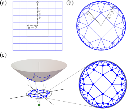
Before constructing hyperbolic lattices, We need to specify the coordinates under which we are handling our studies. To assign a complex coordinate to each lattice site, we employ a conformal disk model of hyperbolic space, i.e., Poincaré disk as shown in the right-hand side of Fig. 1(c). By using this conformal map, the lattice is embedded in a unit disk with metric
| (1) |
where is the constant radius curvature and its corresponding constant curvature is . From Eq. (1), the geodesic distance between two sites and on the Poincaré disk is given by
| (2) |
where denotes a site on the disk with complex coordinate .
II.2 Hyperbolic lattice construction and the exponential wall
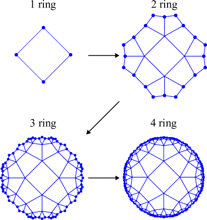
Next, we consider using the regular tilings to generate hyperbolic lattices. By adopting the vertex inflation method (or vertex-inflation tiling procedure) [46, 47, 38], we can effectively generate Euclidean and hyperbolic lattices of various rings where the sites are located. To obtain a finite lattice, we initially generate a regular -edges polygon at the center of the Poincaré disk, labeled as the first ring and then attach new rings to it iteratively. In Fig. 2 we show the generating procedure of lattice, where the bold sites denote the outermost ring that generated in each iterative step. By repeating this process, we can successively enlarge the size of the lattice based on the outermost ring, allowing us to obtain an arbitrarily large lattice with any number of rings. More detailed information on this procedure can be found in Appendix A.
In the following, we use rather than to label a concrete finite hyperbolic lattice, i.e., flake, for numerical computations, where the integer represents the number of rings included in the lattice, as shown in Fig. 1(a) and (b) plotted by the dash line. An important feature of hyperbolic lattice is that the total number of lattice sites increases exponentially with the number of ring as , where is a parameter depending on specific . In contrast, for Euclidean lattices, . Additionally, the number of sites on the outermost ring of the hyperbolic lattice, which corresponds to the boundary, also increases exponentially with for large , whereas in Euclidean lattices, it increases linearly as . A brief proof of these properties can be found in Appendix A, highlighting the fundamental differences between the two geometry. These properties all bring difficulties for numerical computations.
II.3 Partition of subsystems on the hyperbolic lattice
Since the choice of subsystem affects EE, we now turn to specify our partition methods. When partitioning subsystems to study EE, we need to choose the largest possible subsystems while keeping them as far from the boundary as possible to minimize finite-size effect. However, as explained in Sec. II.2, and grow exponentially with , making it difficult to have a relatively large bulk. We define as the shortest discrete graph path from a bulk site to the boundary. Sites with larger than a certain threshold can be chosen to form a single-connected region as , thereby positioning the subsystem on the inner rings of the lattice. Regarding the symmetry of the subsystems, on Euclidean lattices, subsystems are typically chosen as a series of polygons similar to the overall system. However, the symmetry of hyperbolic lattice, described by the triangle group and the Fuchsian group, is non-Abelian [42, 43, 44]. Consequently, the subsystems cannot maintain the same symmetries as on the Euclidean lattice.
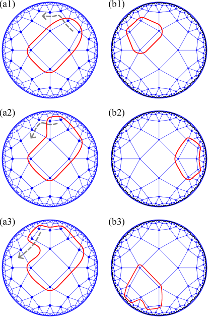
Therefore, we employ two different partition methods in this work. We first generate a lattice of fixed size, within which we choose the sites of the innermost ring as the initial subsystem , and then successively increase its size by adding sites of the adjacent ring to it in a clockwise or anti-clockwise direction. This iterative procedure, which generates a sequential series of subsystems, is visualized in Fig. 3(a), and is referred to as partition i. Additionally, we also conduct a random partition of subsystem. We determine a minimum for a considered lattice and generate subsystem within this region. We first randomly choose a -edges polygon, then enlarge it by successively adhering -edges polygons around sites on the boundary of the subsystem to it and repeat this procedure until it reaches a specific size. This partition method is referred to as partition ii and can be visualized in Fig. 3(b). Since the partitions do not consistently preserve the symmetries of the subsystems, we find that through partition ii the symmetries do not significantly affect the numerical results of EE in practical computations. In the remaining part of the main text, we consistently exhibit the results of EE computed through partition i on some lattices and provide the supplemental data in Appendix B for more details of both partition i and partition ii.
II.4 Entanglement entropy and Widom conjecture
Next, we concisely review some basic algebras for computing the entanglement of free-fermion systems. A useful relevant material can be found in the supplementary note of Ref. [52]. For a many-body system with ground state , its density matrix is . We partition the system into two parts as subsystem of the overall system and its complementary in real space, and obtain reduced density matrix of subsystem by tracing over :
| (3) |
where is a normalization constant and is the entanglement Hamiltonian, from which we can obtain EE [56, 57, 58]. If we consider free-fermion systems, has quadratic form [59, 60, 61] , where and represent the fermionic creation and annihilation operators at site respectively. Additionally, we can rewrite EE as a trace of matrix-function. Consider the correlation matrix of subsystem which can be obtained by projection operators where and , the EE can be calculated by [60, 58, 61, 62, 63, 64, 65]:
| (4) |
where . Hence we obtain EE of subsystem .
Meanwhile, for gapless systems with codimension-1 Fermi surface, the Widom conjecture provides an analytical result of EE [12, 13]:
| (5) |
where and denote the boundaries of the Fermi surface and the subsystem we consider, and denote the exterior unit normals of these boundaries. Since the presence of codimension-1 Fermi surface implies finite DOS of the system, Eq. (5) also relates the DOS to the scaling coefficient. If the codimension of the Fermi surface is higher than one, the leading term of EE exhibits area law scaling behavior, as seen in the Dirac point of tight-binding model on the honeycomb lattice [7, 66, 67]. However, the validity of Eq. (5) requires a Euclidean metric with Abelian translation symmetry and thus is not naturally applicable in the hyperbolic geometry, so we aim to provide numerical evidence in this paper.
III Entanglement entropy scaling of gapless free-fermion systems with finite DOS
III.1 Numerical study of DOS
In this section, we numerically study the scaling behavior of EE of gapless free-fermion systems with finite DOS on hyperbolic lattice. To begin with, we consider the gapless systems with a one-orbital tight-binding model:
| (6) |
where denotes the nearest-neighboring sites, is the hopping amplitude and is the chemical potential. First, we should verify that the Hamiltonian is indeed gapless. We notice that the DOS obtained through exact diagonalization for sites still exhibits finite-size effect, and thus it’s insufficient to verify whether the system is gapless or not through it. Consequently, we analyze DOS in the thermodynamical limit through the Haydock recursion method [48, 49, 50, 51].
One can calculate local DOS at a site through Green’s function:
| (7) |
where is the state we consider and the Green’s function is . The diagonal element of can be expanded in continued-fraction:
| (8) |
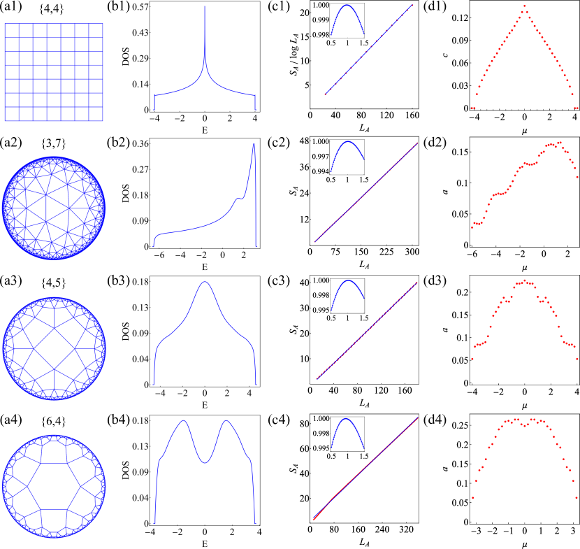
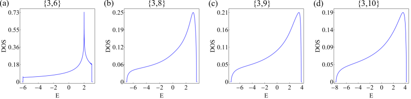
where the rational coefficients and can be numerically computed by the underlying Hamiltonian matrix through specific recursive relation. After introducing a proper fraction termination, we obtain which is also DOS for regular tilings up to a normalization factor [48]. By using this method, we confirm that the Hamiltonian is indeed gapless on lattices that we study here, as shown in Fig. 4(b1-b4). One can refer to Appendix C for more details of this method and numerical results.
III.2 Numerical evidence of area law scaling behavior of EE
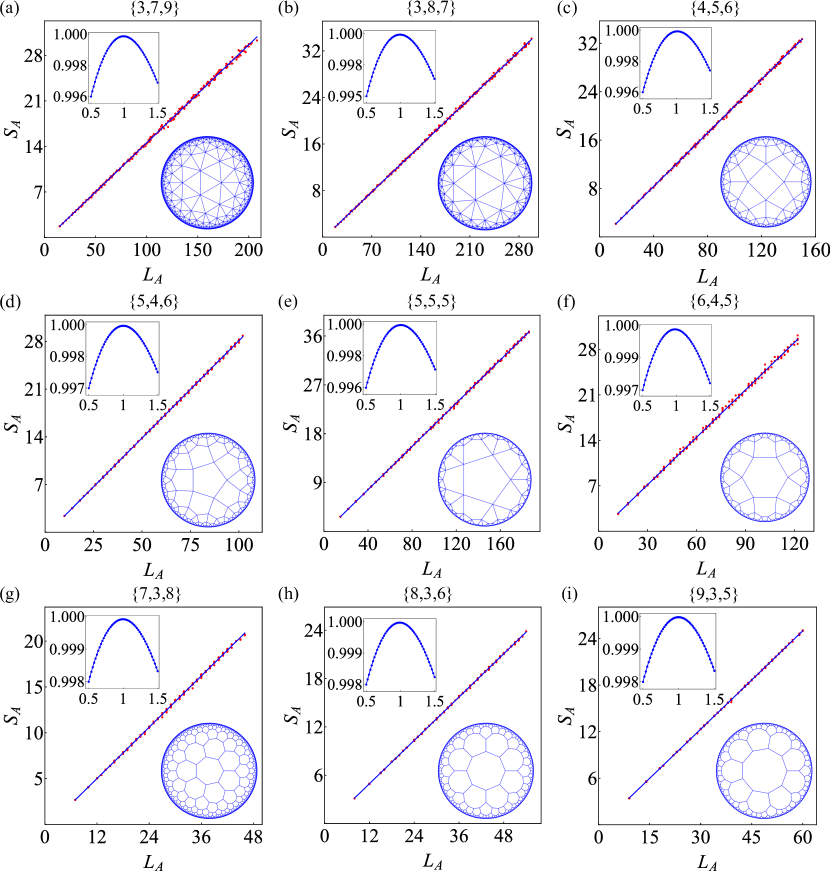
To proceed further, we use our approaches detailed in Sec. II to compute EE on various lattices, including both Euclidean and hyperbolic. In Fig. 4(c2-c4) we show the results computed on , , lattices. Additionally, in Fig. 4(c1), we also include EE computed on Euclidean lattice for comparison. More numerical results through different partition methods on different lattices are detailed in Appendix B.
First, in the Euclidean case, the EE of gapless systems with finite DOS exhibits super-area law, corresponding to our results computed on lattice in Fig. 4(c1), where we anticipate the scaling function . When we turn to the hyperbolic case, our most surprising finding is that the EE of gapless systems with finite DOS is proportional to the length of the boundary of subsystem . We anticipate that the scaling of EE should have . By using the coefficient of determination , we find that is the optimal fit closest to , as shown in Fig. 4(c2-c4). The blue lines in Fig. 4(c) show the fitting functions with . This result indicates that the EE of gapless systems with finite DOS on hyperbolic lattices unexpectedly satisfies the area law:
| (9) |
where represents the total number of bonds connecting a site inside the subsystem to a site outside the subsystem which are cut by the boundary of the subsystem , as visualized in Fig. 3.
With more numerical computations, as illustrated in Appendix B, we further confirm the existence of area law of EE for gapless ground states with finite DOS on hyperbolic lattice. Furthermore, we want to ask why this exotic area law of EE appears in hyperbolic systems. On Euclidean lattice, following Swingle’s (mode-counting) argument [14], for free-fermion systems with codimension-1 Fermi surface, EE can be obtained by counting the contributions of d fermionic gapless modes near the Fermi surface perpendicular to the boundary of the subsystem in real space, where each fermionic gapless mode contributes to EE by adopting the calculation of CFT. Then, we obtain that EE satisfies in Euclidean case. On hyperbolic lattices, the gapless system with finite DOS still has infinite gapless fermionic modes near Fermi level despite the absence of “Fermi surface” of the usual definition. If we can stack and count the contribution of these infinite fermionic gapless modes for EE, we can obtain the scaling behavior of EE for hyperbolic systems. However, there is a lack of a realizable stacking and counting way on hyperbolic lattice. According to Eq. (4), EE depends on the projectors and . HBT provides an insight for us into the parameterization of the generalized hyperbolic Brillouin zone and non-Abelian Bloch states [42, 43, 35, 44, 33]. Therefore, our numerical simulation raises questions and challenges for HBT to obtain a generalized Widom conjecture for hyperbolic lattices, as well as the expressions of and from the parameterized momentum space.
Moreover, the scaling behavior of EE is related to the non-local properties of the systems; therefore, the super-area law behavior of EE indicates that fermionic statistics enhances entanglement in Euclidean geometry. Due to the absence of the logarithmic correction of EE in Eq. (9), we realize that the gapless fermions in hyperbolic lattices should have exotic behavior. Additionally, as hyperbolic geometry suppress entanglement, it is worth investigating the asymptotic behavior of EE with respect to and we discuss this in Appendix D. In the forthcoming Sec. III.3, we will continue to discuss our numerical findings, especially focusing on the scaling coefficient.
III.3 Numerical study of scaling coefficient and possibility of a generalized Widom conjecture
In the Euclidean case, we know from Eq. (5) that the scaling coefficient of the super-area law is determined by the geometry of the codimension-1 Fermi surface in momentum space and the partition of subsystems in real space, and thus is related to DOS, as visualized in Fig. 4(d1). From this perspective, we question whether DOS can affect the coefficient in area law for systems on hyperbolic lattice, and thus consider its dependence on the DOS.
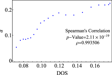
We compute EE for Hamiltonian with and different chemical potential on different hyperbolic lattices. Fig. 4(d2-d4) shows the dependence of the scaling coefficient on . Compared to the DOS computed in Fig. 4(b2-b4), we can directly see that the scaling coefficient is positively related to DOS. In Fig. 5, we present the result computed on lattice as an example, where the Spearman’s correlation indicates a positive monotonic relationship between and the DOS. However, from Fig. 4, we can see that and the DOS do not completely coincide. This discrepancy might also be due to the finite-size effect, as the EE computed here is obtained from a finite lattice while the DOS is obtained in the thermodynamical limit.
In the Euclidean system, the validity of the Widom conjecture needs a Euclidean metric and the momentum space with dimension equal to real-space dimension due to the flux factor in Eq. (5) counting the number of fermionic modes perpendicular to the real space boundary of the subsystem. For the hyperbolic case, since scaling coefficient of area law exhibits similar dependence on DOS, we can also speculate whether there is a similar momentum space and generalized Fermi surface that determines . In fact, the translation group of hyperbolic lattice is typically non-Abelian, resulting in the existence of higher-dimensional () irreducible representations of translation group and non-Abelian Bloch states. Meanwhile, even for the d irreducible representations, the dimension of the generalized Brillouin zone can be [42, 43, 44], which is larger than the spatial dimension of the lattice, thus Swingle’s argument breaks down directly. To exactly obtain a description of reciprocal space of hyperbolic lattice, one needs to know about the higher-dimensional representations. It is an open question that whether we can obtain a generalized Widom conjecture for hyperbolic lattice.
IV Entanglement entropy scaling of gapped free-fermion systems
In this section, we study EE in gapped systems. We consider the gapped systems by studying a two-orbital tight-binding model:
| (10) |
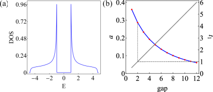
where represents fermionic creation operator at the -orbital of site . and are hopping amplitudes. We can still use Haydock recursion method to compute DOS and verify that is gapped as we did in Sec III. For instance,in Fig. 7(a), we show the DOS of Hamiltonian with and on lattice, which lead to a gapped region .
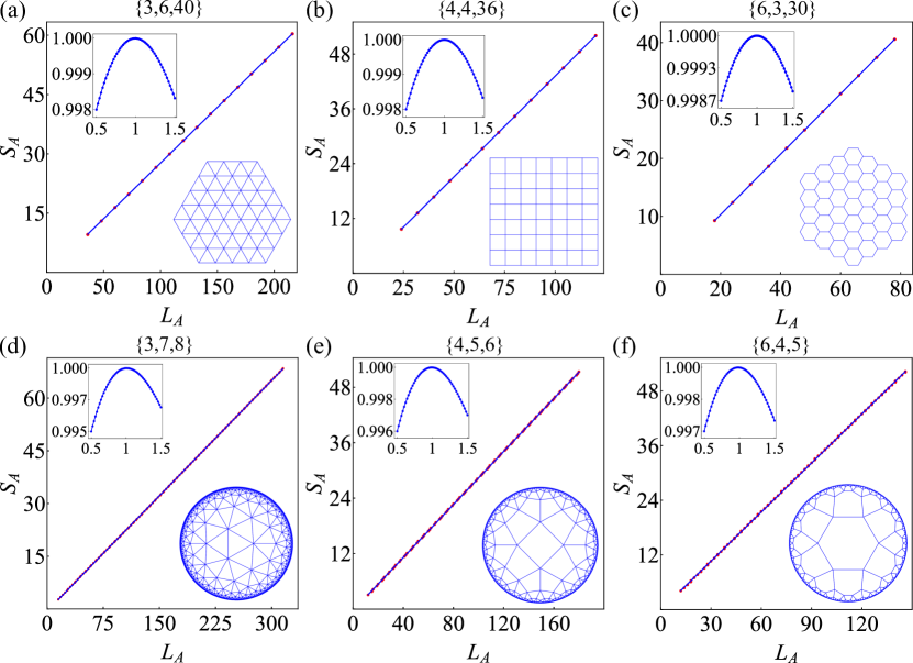
Next, we turn to study EE in gapped case. On Euclidean lattice, EE of gapped systems scales as area law . As an analogy, we also use the fitting function for the case on hyperbolic lattice. In Fig. 6, we show results of EE computed on both Euclidean and hyperbolic lattices. The chosen hyperbolic lattices , and have one more adjacent site per lattice site compared to their Euclidean counterparts , and respectively. The numerical results consistently show that when the the system is gapped, the optimal fit is obtained with where is closest to . The blue lines in Fig. 6 show the fitting functions with . This means that the EE scales linearly with the subsystem’s boundary :
| (11) |
Therefore, EE still scales according to area law in gapped systems on hyperbolic lattice.
.
Additionally, on Euclidean lattices, the coefficient decreases as the energy gap increases. This leads us to question whether the energy gap is related to the behavior of EE. In Fig. 7(b), we study the relation between EE and energy gap on lattice. We modulate and thus change energy gap of from to and compute EE. We find that is negatively correlated with the system’s energy gap. Analytical work on the one-dimensional gapped system has provided a rigorous relationship between the coefficient and the energy gap [68, 2]. However, the exact relationship between the scaling coefficient and the energy gap is still a difficult question in dimension . In our results, we do not find a functional relationship that can physically explain the relationship between the coefficient and the energy gap in the hyperbolic case, but the observed negative monotonic relationship between them suggests a similarity to the Euclidean case.
Overall, our numerical data computed in gapped systems demonstrates that the EE scales according to area law as in Eq. (11). This aligns with our expectations from the Euclidean case, suggesting that the gapped scenario in the hyperbolic case is not particularly unique.
V Discussions
In this paper, we have numerically studied the scaling behavior of entanglement entropy of gapped free fermions as well as gapless free fermions with finite DOS on hyperbolic lattice. We find that for both gapped and gapless systems, the EE scales according to a rigorous area law scaling . Although the gapped case fulfills our expectation in Euclidean geometry, the super-area law in gapless systems breaks down in contrast. Additionally, the scaling coefficient of area law in gapless systems is positively related to the DOS. This scaling behavior of EE is unique in hyperbolic geometry. On Euclidean lattice, the super-area law of gapless free fermions with finite DOS demonstrates that the entanglement is enhanced by the fermionic statistics and the quantum correlation of the infinite fermion modes near the Fermi surface [12, 14]. Compared to Euclidean case, the area law of gapless systems on hyperbolic lattices suggests the exotic properties induced by the hyperbolic geometry and the generalization of Widom conjecture to hyperbolic lattices. The generalized Bloch theory, or hyperbolic band theory (HBT), of hyperbolic lattice could provide a description through representation theory for non-Abelian translation group of hyperbolic lattice, thereby describing the generalized momentun space and may yield a momentun space formula for EE [43, 42, 44].
Moreover, we find that the EE of a free-fermion system behaves differently under different geometries, reflecting the nature of the spatial geometry where the system is embedded, e.g., fractal lattice discussed in Ref. [45]. As it is feasible to simulate entanglement experimentally [52] while the photonic and circuit experimental realization of hyperbolic lattice has been achieved [27, 26, 30, 28, 29, 31], this may provide us with a novel approach to study the geometry of the quantum system through entanglement. Additionally, the area law of EE in both gapped and gapless systems suggests that it is efficient to study correlated systems on hyperbolic lattices with gapless emergent fermions by tensor-network-type numerical techniques [53, 18, 54]. We hope that our work can provide some inspiration to related fields in the future. Another interesting future direction is to study entanglement of non-Hermitian systems [69, 70, 64, 65, 71, 72, 73, 74, 75, 76, 77, 78, 79, 80, 81, 82, 83, 84, 85, 86, 87] on hyperbolic lattice, which is much more practical in, e.g., phononic systems where gain and loss are natural.
Acknowledgements.
This work was supported by National Natural Science Foundation of China (NSFC) Grant No. 12074438 and Guangdong Provincial Key Laboratory of Magnetoelectric Physics and Devices under Grant No. 2022B1212010008.Appendix A Hyperbolic lattice
In this section we give details of constructing hyperbolic lattices discussed in Sec. II.
A.1 Vertex inflation method of generating hyperbolic lattice
The vertex inflation method or vertex-inflation tiling procedure for generating hyperbolic lattice was first purposed in the field of hyperbolic tensor-network theory [46, 47] and then optimized for study in lattice many-body models [38]. Here, we introduce our lattice set-up based on this method.
To start with, we generate a regular -edges polygon at the center of the Poincaré disk and denote it as the -st ring of the lattice. We then attach new sites to the -st ring to form a new ring, and iteratively repeat this procedure. This finite-size lattices, named as flakes, can be divided into rings in order and every regular -edges polygon is denoted as a tile. For every vertex of a tile, the vertex is affiliated to this tile. If a vertex doesn’t have affiliated tile it is an open vertex. A vertex with neighboring vertices does not equal to not open since it may have less than affiliated tiles. If an open vertex has an nearest-neighboring vertex which is also open, the edge linking them is an open edge. The lattice set-up procedure is summarized as follows:
-
1.
For a lattice, we find all open vertices and their corresponding open edge on its outermost -th ring. A vertex on -th ring can either have zero or two open edge of which it is an endpoint.
-
2.
For every open vertex and one of its open edge, if its number of affiliated tiles is less than , we identify the tile to which the open edge belongs and invert this tile. This process creates a new tile and an new open edge of which is an endpoint.
-
3.
Otherwise, for every open vertex with affiliated tiles, we identify both two open edges it belongs to and generate a new tile based on them.
-
4.
Go back to step one and repeat the whole process until all vertices on the -th ring are no longer open. So far we have constructed a new ring and lattice.
By using the above method, we can construct the entire lattice ring by ring. The procedure can be visualized as Fig. 2. The finite lattice generated by this method do not have dangling sites on the inner rings and it is natural to define the outermost ring as the boundary.
A.2 Exponential growth of the size of the hyperbolic lattice
In this section, we give a brief proof of the exponential growth of the size of hyperbolic lattice. We start by considering lattice with and . The proofs for the remaining cases are similar to the following proof.
For a lattice , all vertices on the outermost ()-th ring can have either or nearest neighboring vertices to which is connected by an edge. We denote as the number of vertices on the -th ring. The number of vertices having nearest neighboring vertices on the outermost ring is denoted as , and the number of vertices having nearest neighboring vertices on the outermost ring is denoted as by analogy. Thus we have:
| (12) |
for any .
In the procedure of generating the lattice, the construction of -th ring is only dependent on the ()-th ring. Every -neighboring vertex on the ()-th ring directly has neighboring vertices on the -th ring, and these vertices form tiles which need new vertices each. Similarly, every -neighboring vertex on the ()-th ring directly has neighboring vertices on the -th ring. These new neighboring vertices form tiles which need new vertices each.
Besides, the edges on the ()-th ring, whose number is equal to , form tiles, each of which requires new vertices. Summarizing the above constraints, we have:
| (13) |
We also notice that each -neighboring vertex on the ()-th ring is directly connected to a vertex on ()-th ring. That is:
for any . And for -neighboring vertex, the case is:
Summarizing the above results, we get the recursive relation:
| (14) |
Solving this relation is equivalent to find the root of quadratic equation
| (15) |
for . As we directly have and , by solving above equation we find the formula of , as
| (16) |
where . Finally summing over all the rings yields exponentially growing size of lattice:
| (17) |
where depends on specific and can be analytically calculated.
This shows an exponential growth of lattice size which is absolutely different from Euclidean case since Euclidean lattice grows as . Some lattices are shown in Table. 1, from which we can see the difference between hyperbolic case and Euclidean case.
| lattice | 1st | 2nd | 3rd | 4th | 5th | 6th |
| 3 | 12 | 33 | 87 | 228 | 597 | |
| 4 | 20 | 76 | 284 | 1060 | 3956 | |
| 6 | 42 | 246 | 1434 | 8358 | 48714 | |
| 8 | 40 | 152 | 568 | 2120 | 7912 | |
| 8 | 280 | 9512 | 323128 | - | - | |
| lattice | 1st | 5th | 10th | 100th | - | - |
| 3 | 27 | 57 | 597 | |||
| 4 | 36 | 76 | 796 | |||
| 6 | 54 | 114 | 1194 |
Appendix B Supplemental data of numerical computations of EE through partition i and partition ii
As detailed in Sec. II, when studying EE, we use some different partition methods to investigate how the EE varies with the boundary as the size of the subsystem changes.
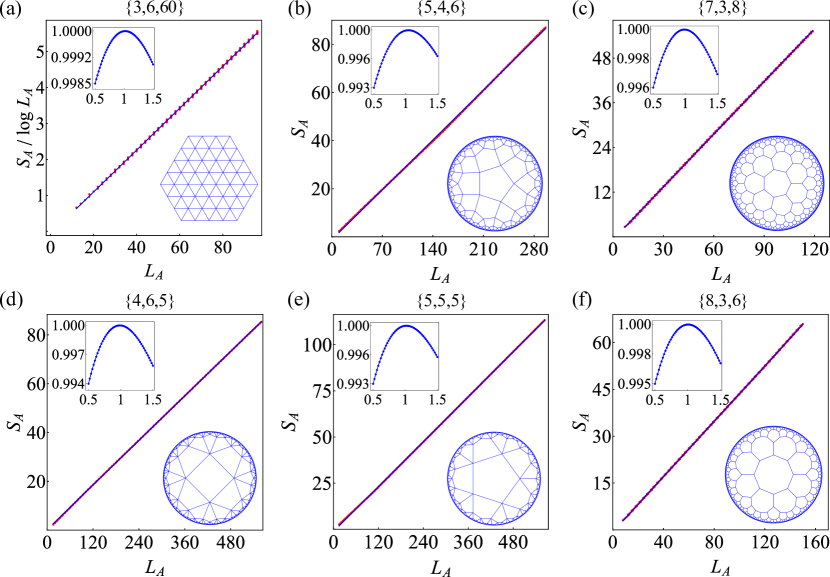
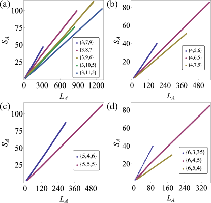
The supplemental data of EE computed through partition i with and for Hamiltonian on lattices different from those in the main text can be seen in Fig. 8. Here we anticipate the scaling function for Euclidean lattice which exhibit super-area law that can be seen in Fig. 8(a) while the hyperbolic cases all exhibit area law and we anticipate the scaling of EE is . On Euclidean lattices, increasing subsystems size successively can result in many subsystems with different shapes and sizes sharing the same , e.g., lattice in Fig. 8(a). In the main text the size of subsystem on Euclidean lattices grows discretely so that we have subsystems similar to the overall system. However, enlarging the size of the subsystem successively causes to increase successively in the hyperbolic case, as shown in Fig. 8(b-f). This enable us to study the growth of EE with the successively increasing boundary with numerous data, regardless of the exponential wall of the lattice size. Although this partitioning method may not maintain the symmetries, it still significantly distinguishes between area law and super-area law behavior of EE.
The results of EE computed through partition ii are exhibited in Fig. 9, where we use fitting function . Because choosing subsystems too close to the boundary will cause finite-size effect, we define an internal region of the lattice, specify the size of subsystems and then randomly choose subsystems that can be composed of connected tiles. The results in Fig. 9 are computed with Hamiltonian and we set and , as are those shown in Fig. 8, and the blue lines show the fitting functions with . Even with the same size or the same , subsystems partitioned through this method can have various possible shapes and do not maintain the same symmetries. However, the symmetries of these subsystems do not affect the scaling behavior of EE. From the results, we find that linearity still demonstrates that the best description between EE and boundary is area law.
Appendix C Numerical study of DOS
Based on our considerations in the main text, we need to verify that the Hamiltonian is indeed gapless on lattices we considered. Because the geometric properties of hyperbolic lattice induce exotic behavior of free fermions, we use DOS as the verification.
Additionally, as aforementioned, the size of the system grows exponentially with , resulting numerical difficulties in exact diagonalization (ED) approach. Therefore, we use the Haydock recursion method [49, 50, 88, 51, 89, 48] to acquire DOS in the thermodynamical limit.
C.1 Haydock recursion approach to DOS
We can calculate local density-of-states (LDOS) at a particular site by Green’s function:
| (18) |
The Green’s function can be decomposed into contributions from moments of the Hamiltonian .
The Haydock recursion method [49, 50, 51], also known as the continued-fraction method, give a method to compute the diagonal matrix element of :
| (19) |
Here is a unit vector that has non-zero component at site only. The rational continued-fraction coefficients and in Eq. (C.1) can be obtained by the following recursive relation:
| (20) |
where and . For gapless systems, the coefficients and converge to the asymptotic value and for sufficiently large lattices and give the band edges:
| (21) |
For gapped systems with single band gap, which is the case of Hamiltonian , the coefficients converges to two asymptotic limit and when [88]:
| (22) |
where is band gap.
To accurately compute the rational coefficients and to the order , the shortest graphic path from site to boundary as defined in Sec. II should be at least . Then we introduce a proper fraction termination:
| (23) |
for Hamiltonian , where and are chosen as the converged and for large . In gapped system the fraction termination can be more complicated [88, 89], for Hamiltonian we use:
| (24) |
where , , and are band edges which can be obtained by the asymptotic coefficient in Eq. C.1.
C.2 Numerical results of DOS
We show some results of DOS which are computed on different lattices with up to sites for Hamiltonian in Fig. 10. Here we compute DOS on lattices and verify that they are gapless. Since this method’s memory consumption scales linearly with the lattice size, it significantly exceeds the computational limits of ED methods. This method can be applied to arbitrarily large lattice (one can obtain result for lattice size up to sites [48]) but our results here are sufficient to determine whether the system is gapped or gapless in the thermodynamical limit.
We notice that the thermodynamical DOS obtained through this method is different from that computed on finite lattices through ED, indicating that the computation of EE may exhibit finite-size effect.
Appendix D Asymptotic behavior of scaling coefficient of area law
In this section, we study how EE varies with when is fixed. The number of nearest neighboring sites of a given site on hyperbolic lattice, labeled as as aforementioned, can increase successively. From our findings in the main text, EE is proportional to the boundary of subsystem , which is a function of , thus the area-law scaling coefficient should also be related to . We study EE for Hamiltonian on and hyperbolic lattices with successively increased and the results are shown in Fig. 11. The results all indicate that as the number of adjacent sites per site increases, the coefficient decreases.
Due to computational difficulties on hyperbolic lattices, such as the exponentially growing lattice size and finite-size effect, it is hard to perform the scaling analysis for lattice with larger . However, our results here indicate a monotonically decreasing relationship between and . It makes sense to explore the relationship of as increases, as this may reveal the asymptotic behavior of EE and provide us an new insights into the hyperbolic geometry.
References
- Amico et al. [2008] L. Amico, R. Fazio, A. Osterloh, and V. Vedral, Entanglement in many-body systems, Rev. Mod. Phys. 80, 517 (2008).
- Eisert et al. [2010] J. Eisert, M. Cramer, and M. B. Plenio, Colloquium: Area laws for the entanglement entropy, Rev. Mod. Phys. 82, 277 (2010).
- Laflorencie [2016] N. Laflorencie, Quantum entanglement in condensed matter systems, Physics Reports 646, 1 (2016).
- Calabrese and Cardy [2004] P. Calabrese and J. Cardy, Entanglement entropy and quantum field theory, Journal of Statistical Mechanics: Theory and Experiment 2004, P06002 (2004).
- Abanin et al. [2019] D. A. Abanin, E. Altman, I. Bloch, and M. Serbyn, Colloquium: Many-body localization, thermalization, and entanglement, Rev. Mod. Phys. 91, 021001 (2019).
- Li et al. [2006] W. Li, L. Ding, R. Yu, T. Roscilde, and S. Haas, Scaling behavior of entanglement in two- and three-dimensional free-fermion systems, Phys. Rev. B 74, 073103 (2006).
- Barthel et al. [2006] T. Barthel, M.-C. Chung, and U. Schollwöck, Entanglement scaling in critical two-dimensional fermionic and bosonic systems, Phys. Rev. A 74, 022329 (2006).
- Zhou and Ye [2023] Y. Zhou and P. Ye, Entanglement signature of hinge arcs, fermi arcs, and crystalline symmetry protection in higher-order weyl semimetals, Phys. Rev. B 107, 085108 (2023).
- Holzhey et al. [1994] C. Holzhey, F. Larsen, and F. Wilczek, Geometric and renormalized entropy in conformal field theory, Nuclear Physics B 424, 443–467 (1994).
- Calabrese and Cardy [2009] P. Calabrese and J. Cardy, Entanglement entropy and conformal field theory, Journal of Physics A: Mathematical and Theoretical 42, 504005 (2009).
- Widom [1982] H. Widom, On a class of integral operators with discontinuous symbol, in Operator Theory: Advances and Applications (Birkhäuser Basel, 1982) p. 477–500.
- Gioev and Klich [2006] D. Gioev and I. Klich, Entanglement entropy of fermions in any dimension and the widom conjecture, Phys. Rev. Lett. 96, 100503 (2006).
- Leschke et al. [2014] H. Leschke, A. V. Sobolev, and W. Spitzer, Scaling of rényi entanglement entropies of the free fermi-gas ground state: A rigorous proof, Phys. Rev. Lett. 112, 160403 (2014).
- Swingle [2010] B. Swingle, Entanglement entropy and the fermi surface, Phys. Rev. Lett. 105, 050502 (2010).
- Magnus [1974] W. Magnus, Noneuclidean Tesselations and Their Groups, Pure and Applied Mathematics, Vol. 61 (Academic Press, New York, 1974).
- Maldacena [1998] J. Maldacena, The large limit of superconformal field theories and supergravity, Adv. Theor. Math. Phys. 2, 231 (1998).
- Nishioka [2018] T. Nishioka, Entanglement entropy: Holography and renormalization group, Rev. Mod. Phys. 90, 035007 (2018).
- Cirac et al. [2021] J. I. Cirac, D. Pérez-García, N. Schuch, and F. Verstraete, Matrix product states and projected entangled pair states: Concepts, symmetries, theorems, Rev. Mod. Phys. 93, 045003 (2021).
- Brower et al. [2021] R. C. Brower, C. V. Cogburn, A. L. Fitzpatrick, D. Howarth, and C.-I. Tan, Lattice setup for quantum field theory in , Phys. Rev. D 103, 094507 (2021).
- Asaduzzaman et al. [2020] M. Asaduzzaman, S. Catterall, J. Hubisz, R. Nelson, and J. Unmuth-Yockey, Holography on tessellations of hyperbolic space, Phys. Rev. D 102, 034511 (2020).
- Brower et al. [2022] R. C. Brower, C. V. Cogburn, and E. Owen, Hyperbolic lattice for scalar field theory in , Phys. Rev. D 105, 114503 (2022).
- Mück and Viswanathan [1998a] W. Mück and K. S. Viswanathan, Conformal field theory correlators from classical scalar field theory on anti–de sitter space, Phys. Rev. D 58, 041901 (1998a).
- Mück and Viswanathan [1998b] W. Mück and K. S. Viswanathan, Conformal field theory correlators from classical field theory on anti–de sitter space: Vector and spinor fields, Phys. Rev. D 58, 106006 (1998b).
- Henningson and Sfetsos [1998] M. Henningson and K. Sfetsos, Spinors and the AdS/CFT correspondence, Physics Letters B 431, 63 (1998).
- [25] G. Shankar and J. Maciejko, Hyperbolic lattices and two-dimensional yang-mills theory, arXiv:2309.03857 .
- [26] S. Dey, A. Chen, P. Basteiro, A. Fritzsche, M. Greiter, M. Kaminski, P. M. Lenggenhager, R. Meyer, R. Sorbello, A. Stegmaier, R. Thomale, J. Erdmenger, and I. Boettcher, Simulating holographic conformal field theories on hyperbolic lattices, arXiv:2404.03062 .
- Kollár et al. [2019] A. J. Kollár, M. Fitzpatrick, and A. A. Houck, Hyperbolic lattices in circuit quantum electrodynamics, Nature 571, 45–50 (2019).
- Yu et al. [2020] S. Yu, X. Piao, and N. Park, Topological hyperbolic lattices, Phys. Rev. Lett. 125, 053901 (2020).
- Boettcher et al. [2020] I. Boettcher, P. Bienias, R. Belyansky, A. J. Kollár, and A. V. Gorshkov, Quantum simulation of hyperbolic space with circuit quantum electrodynamics: From graphs to geometry, Phys. Rev. A 102, 032208 (2020).
- Lenggenhager et al. [2022] P. M. Lenggenhager, A. Stegmaier, L. K. Upreti, T. Hofmann, T. Helbig, A. Vollhardt, M. Greiter, C. H. Lee, S. Imhof, H. Brand, T. Kießling, I. Boettcher, T. Neupert, R. Thomale, and T. Bzdušek, Simulating hyperbolic space on a circuit board, Nature Communications 13, 10.1038/s41467-022-32042-4 (2022).
- Huang et al. [2024] L. Huang, L. He, W. Zhang, H. Zhang, D. Liu, X. Feng, F. Liu, K. Cui, Y. Huang, W. Zhang, and X. Zhang, Hyperbolic photonic topological insulators, Nature Communications 15, 10.1038/s41467-024-46035-y (2024).
- Zhu et al. [2021] X. Zhu, J. Guo, N. P. Breuckmann, H. Guo, and S. Feng, Quantum phase transitions of interacting bosons on hyperbolic lattices, Journal of Physics: Condensed Matter 33, 335602 (2021).
- Tummuru et al. [2024] T. Tummuru, A. Chen, P. M. Lenggenhager, T. Neupert, J. Maciejko, and T. c. v. Bzdušek, Hyperbolic non-abelian semimetal, Phys. Rev. Lett. 132, 206601 (2024).
- Liu et al. [2022] Z.-R. Liu, C.-B. Hua, T. Peng, and B. Zhou, Chern insulator in a hyperbolic lattice, Phys. Rev. B 105, 245301 (2022).
- Urwyler et al. [2022] D. M. Urwyler, P. M. Lenggenhager, I. Boettcher, R. Thomale, T. Neupert, and T. c. v. Bzdušek, Hyperbolic topological band insulators, Phys. Rev. Lett. 129, 246402 (2022).
- Liu et al. [2023] Z.-R. Liu, C.-B. Hua, T. Peng, R. Chen, and B. Zhou, Higher-order topological insulators in hyperbolic lattices, Phys. Rev. B 107, 125302 (2023).
- Tao and Xu [2023] Y.-L. Tao and Y. Xu, Higher-order topological hyperbolic lattices, Phys. Rev. B 107, 184201 (2023).
- Chen et al. [2023] A. Chen, Y. Guan, P. M. Lenggenhager, J. Maciejko, I. Boettcher, and T. c. v. Bzdušek, Symmetry and topology of hyperbolic haldane models, Phys. Rev. B 108, 085114 (2023).
- Lux and Prodan [2023] F. R. Lux and E. Prodan, Converging periodic boundary conditions and detection of topological gaps on regular hyperbolic tessellations, Phys. Rev. Lett. 131, 176603 (2023).
- Zhang et al. [2022] W. Zhang, H. Yuan, N. Sun, H. Sun, and X. Zhang, Observation of novel topological states in hyperbolic lattices, Nature Communications 13, 10.1038/s41467-022-30631-x (2022).
- [41] C. Sun, A. Chen, T. Bzdušek, and J. Maciejko, Topological linear response of hyperbolic chern insulators, arXiv:2406.08388 .
- Maciejko and Rayan [2021] J. Maciejko and S. Rayan, Hyperbolic band theory, Science Advances 7, eabe9170 (2021).
- Maciejko and Rayan [2022] J. Maciejko and S. Rayan, Automorphic bloch theorems for hyperbolic lattices, Proceedings of the National Academy of Sciences 119, e2116869119 (2022).
- Lenggenhager et al. [2023] P. M. Lenggenhager, J. Maciejko, and T. c. v. Bzdušek, Non-abelian hyperbolic band theory from supercells, Phys. Rev. Lett. 131, 226401 (2023).
- [45] Y. Zhou and P. Ye, Quantum entanglement on fractal landscapes, arXiv:2311.01199 .
- Boyle et al. [2020] L. Boyle, M. Dickens, and F. Flicker, Conformal quasicrystals and holography, Phys. Rev. X 10, 011009 (2020).
- Jahn et al. [2020] A. Jahn, Z. Zimborás, and J. Eisert, Central charges of aperiodic holographic tensor-network models, Phys. Rev. A 102, 042407 (2020).
- Mosseri and Vidal [2023] R. Mosseri and J. Vidal, Density of states of tight-binding models in the hyperbolic plane, Phys. Rev. B 108, 035154 (2023).
- Haydock et al. [1972] R. Haydock, V. Heine, and M. J. Kelly, Electronic structure based on the local atomic environment for tight-binding bands, Journal of Physics C: Solid State Physics 5, 2845–2858 (1972).
- Haydock and Kelly [1973] R. Haydock and M. Kelly, Surface densities of states in the tight-binding approximation, Surface Science 38, 139 (1973).
- Haydock et al. [1975] R. Haydock, V. Heine, and M. J. Kelly, Electronic structure based on the local atomic environment for tight-binding bands. ii, Journal of Physics C: Solid State Physics 8, 2591 (1975).
- Lin et al. [2024] Z.-K. Lin, Y. Zhou, B. Jiang, B.-Q. Wu, L.-M. Chen, X.-Y. Liu, L.-W. Wang, P. Ye, and J.-H. Jiang, Measuring entanglement entropy and its topological signature for phononic systems, Nature Communications 15, 10.1038/s41467-024-45887-8 (2024).
- Orús [2014] R. Orús, A practical introduction to tensor networks: Matrix product states and projected entangled pair states, Annals of Physics 349, 117 (2014).
- Xiang [2023] T. Xiang, Density Matrix and Tensor Network Renormalization (Cambridge University Press, 2023).
- Boettcher et al. [2022] I. Boettcher, A. V. Gorshkov, A. J. Kollár, J. Maciejko, S. Rayan, and R. Thomale, Crystallography of hyperbolic lattices, Phys. Rev. B 105, 125118 (2022).
- Li and Haldane [2008] H. Li and F. D. M. Haldane, Entanglement spectrum as a generalization of entanglement entropy: Identification of topological order in non-abelian fractional quantum hall effect states, Phys. Rev. Lett. 101, 010504 (2008).
- Fidkowski [2010] L. Fidkowski, Entanglement spectrum of topological insulators and superconductors, Phys. Rev. Lett. 104, 130502 (2010).
- Lee et al. [2014] C. H. Lee, P. Ye, and X.-L. Qi, Position-momentum duality in the entanglement spectrum of free fermions, Journal of Statistical Mechanics: Theory and Experiment 2014, P10023 (2014).
- Klich [2006] I. Klich, Lower entropy bounds and particle number fluctuations in a fermi sea, Journal of Physics A: Mathematical and General 39, L85 (2006).
- Peschel [2003] I. Peschel, Calculation of reduced density matrices from correlation functions, Journal of Physics A: Mathematical and General 36, L205 (2003).
- Lee and Ye [2015] C. H. Lee and P. Ye, Free-fermion entanglement spectrum through wannier interpolation, Phys. Rev. B 91, 085119 (2015).
- Lai and Yang [2015] H.-H. Lai and K. Yang, Entanglement entropy scaling laws and eigenstate typicality in free fermion systems, Phys. Rev. B 91, 081110 (2015).
- Crampé et al. [2019] N. Crampé, R. I. Nepomechie, and L. Vinet, Free-fermion entanglement and orthogonal polynomials, Journal of Statistical Mechanics: Theory and Experiment 2019, 093101 (2019).
- Chen et al. [2021] L.-M. Chen, S. A. Chen, and P. Ye, Entanglement, non-hermiticity, and duality, SciPost Phys. 11, 003 (2021).
- Lee [2022] C. H. Lee, Exceptional bound states and negative entanglement entropy, Phys. Rev. Lett. 128, 010402 (2022).
- Levine and Miller [2008] G. C. Levine and D. J. Miller, Zero-dimensional area law in a gapless fermionic system, Phys. Rev. B 77, 205119 (2008).
- Ding et al. [2008] L. Ding, N. Bray-Ali, R. Yu, and S. Haas, Subarea law of entanglement in nodal fermionic systems, Phys. Rev. Lett. 100, 215701 (2008).
- Hastings [2007] M. B. Hastings, An area law for one-dimensional quantum systems, Journal of Statistical Mechanics: Theory and Experiment 2007, P08024 (2007).
- Herviou et al. [2019] L. Herviou, N. Regnault, and J. H. Bardarson, Entanglement spectrum and symmetries in non-Hermitian fermionic non-interacting models, SciPost Phys. 7, 069 (2019).
- Chang et al. [2020] P.-Y. Chang, J.-S. You, X. Wen, and S. Ryu, Entanglement spectrum and entropy in topological non-hermitian systems and nonunitary conformal field theory, Phys. Rev. Res. 2, 033069 (2020).
- Modak and Mandal [2021] R. Modak and B. P. Mandal, Eigenstate entanglement entropy in a -invariant non-hermitian system, Phys. Rev. A 103, 062416 (2021).
- Guo et al. [2021] Y.-B. Guo, Y.-C. Yu, R.-Z. Huang, L.-P. Yang, R.-Z. Chi, H.-J. Liao, and T. Xiang, Entanglement entropy of non-hermitian free fermions, Journal of Physics: Condensed Matter 33, 475502 (2021).
- Tu et al. [2022] Y.-T. Tu, Y.-C. Tzeng, and P.-Y. Chang, Rényi entropies and negative central charges in non-Hermitian quantum systems, SciPost Phys. 12, 194 (2022).
- Ortega-Taberner et al. [2022] C. Ortega-Taberner, L. Rødland, and M. Hermanns, Polarization and entanglement spectrum in non-hermitian systems, Phys. Rev. B 105, 075103 (2022).
- Chen et al. [2022] L.-M. Chen, Y. Zhou, S. A. Chen, and P. Ye, Quantum entanglement of non-hermitian quasicrystals, Phys. Rev. B 105, L121115 (2022).
- Kawabata et al. [2023] K. Kawabata, T. Numasawa, and S. Ryu, Entanglement phase transition induced by the non-hermitian skin effect, Phys. Rev. X 13, 021007 (2023).
- Zou et al. [2023] Y.-Y. Zou, Y. Zhou, L.-M. Chen, and P. Ye, Detecting bulk and edge exceptional points in non-hermitian systems through generalized petermann factors, Frontiers of Physics 19, 10.1007/s11467-023-1337-8 (2023).
- Gal et al. [2023] Y. L. Gal, X. Turkeshi, and M. Schirò, Volume-to-area law entanglement transition in a non-Hermitian free fermionic chain, SciPost Phys. 14, 138 (2023).
- Hsieh and Chang [2023] C.-T. Hsieh and P.-Y. Chang, Relating non-Hermitian and Hermitian quantum systems at criticality, SciPost Phys. Core 6, 062 (2023).
- Yi et al. [2023] W.-Z. Yi, Y.-J. Hai, R. Xiao, and W.-Q. Chen, Exceptional entanglement in non-Hermitian fermionic models, arXiv e-prints , arXiv:2304.08609 (2023), arXiv:2304.08609 [quant-ph] .
- Zhou [2024a] L. Zhou, Entanglement phase transitions in non-hermitian quasicrystals, Phys. Rev. B 109, 024204 (2024a).
- Li et al. [2024] S.-Z. Li, X.-J. Yu, and Z. Li, Emergent entanglement phase transitions in non-hermitian aubry-andré-harper chains, Phys. Rev. B 109, 024306 (2024).
- Zhou [2024b] L. Zhou, Entanglement phase transitions in non-hermitian floquet systems, Phys. Rev. Res. 6, 023081 (2024b).
- Xue and Lee [2024] W.-T. Xue and C. H. Lee, Topologically protected negative entanglement, arXiv e-prints , arXiv:2403.03259 (2024), arXiv:2403.03259 [quant-ph] .
- Shi et al. [2024] S. Shi, L. Dong, J. Bao, and B. Guo, Entanglement entropy and topological properties in a long-range non-hermitian su–schrieffer–heeger model, Physica B: Condensed Matter 674, 415601 (2024).
- Munoz-Arboleda et al. [2024] D. F. Munoz-Arboleda, R. Arouca, and C. Morais Smith, Thermodynamics and entanglement entropy of the non-Hermitian SSH model, arXiv e-prints , arXiv:2406.13087 (2024), arXiv:2406.13087 [quant-ph] .
- Yang et al. [2024] Z. Yang, C. Lu, and X. Lu, Entangelment Entropy on Generalized Brillouin Zone, arXiv e-prints , arXiv:2406.15564 (2024), arXiv:2406.15564 [cond-mat.mes-hall] .
- Gaspard and Cyrot-Lackmann [1973] J. P. Gaspard and F. Cyrot-Lackmann, Density of states from moments. application to the impurity band, Journal of Physics C: Solid State Physics 6, 3077 (1973).
- Haydock and Nex [1984] R. Haydock and C. M. M. Nex, Comparison of quadrature and termination for estimating the density of states within the recursion method, Journal of Physics C: Solid State Physics 17, 4783 (1984).