Signal-SGN: A Spiking Graph Convolutional Network for Skeletal Action Recognition via Learning Temporal-Frequency Dynamics

Abstract

In skeletal-based action recognition, Graph Convolutional Networks (GCNs) based methods face limitations due to their complexity and high energy consumption. Spiking Neural Networks (SNNs) have gained attention in recent years for their low energy consumption, but existing methods combining GCNs and SNNs fail to fully utilize the temporal characteristics of skeletal sequences, leading to increased storage and computational costs. To address this issue, we propose a Signal-SGN(Spiking Graph Convolutional Network), which leverages the temporal dimension of skeletal sequences as the spiking timestep and treats features as discrete stochastic signals. The core of the network consists of a 1D Spiking Graph Convolutional Network (1D-SGN) and a Frequency Spiking Convolutional Network (FSN). The SGN performs graph convolution on single frames and incorporates spiking network characteristics to capture inter-frame temporal relationships, while the FSN uses Fast Fourier Transform (FFT) and complex convolution to extract temporal-frequency features. We also introduce a multi-scale wavelet transform feature fusion module(MWTF) to capture spectral features of temporal signals, enhancing the model’s classification capability. We propose a pluggable temporal-frequency spatial semantic feature extraction module(TFSM) to enhance the model’s ability to distinguish features without increasing inference-phase consumption. Our numerous experiments on the NTU RGB+D, NTU RGB+D 120, and NW-UCLA datasets demonstrate that the proposed models not only surpass existing SNN-based methods in accuracy but also reduce computational and storage costs during training. Furthermore, they achieve competitive accuracy compared to corresponding GCN-based methods, which is quite remarkable.

Introduction

Skeleton-based action recognition is a key area within human action recognition that uses sparse labels generated through pose estimation for classification (Ren et al. 2024). Over time, various methods such as CNN (Du, Fu, and Wang 2015), LSTM (Gao et al. 2022), Transformer (Plizzari, Cannici, and Matteucci 2021), and GCN (Cheng et al. 2020b) have been proposed and have played important roles. ST-GCN (Yan, Xiong, and Lin 2018) was the first to be introduced in skeletal action recognition to capture the spatiotemporal relationships of skeletal sequences, laying the foundation for GCN-based methods. Several methods, such as 2s-AGCN(Shi et al. 2019) and Dynamic GCN(Ye et al. 2020), have improved accuracy. Lightweight models like Shift-GCN(Cheng et al. 2020b) and CTR-GCN(Chen et al. 2021) reduce computational costs while maintaining or enhancing accuracy. Those deep networks with ten-layer pyramid structures increase parameters and energy consumption, conflicting with future energy-saving demands.

SNN is a third-generation neural network designed based on bionics and brain-like computing. It relies on event-driven transmission of features through pulse signals in the form of 0s and 1s (Ghosh-Dastidar and Adeli 2009). SNN is energy-efficient and has been applied in image classification and point cloud estimation(Yamazaki et al. 2022). For example, Spikformer extends static images into the temporal dimension using spiking neurons for information transmission and achieves image classification results through a series of processing layers and a global average-pooling layer. However, some methods overlook the characteristics of spike forms as discrete, aperiodic signals in the temporal domain.(Zhou et al. 2022)

SGN combines graph convolution and spiking neural networks and has been proven to reduce energy consumption by nearly 99% compared to traditional graph convolution networks(Zhu et al. 2022).SGN also has been utilized for skeletal action recognition, achieving impressive results by reducing energy consumption to less than 5% of GCN-based methods while maintaining accuracy. However, current methods treat skeletal sequences as static data, neglecting their temporal characteristics. This introduces additional storage and computational costs, especially with increased temporal steps, making it challenging to train models on standard deep learning devices(Zheng, Xia, and Liang 2024).

We need low-energy, high-accuracy models and minimize additional training consumption due to increased dimensions. We propose a Signal-SGN network for skeletal action recognition. Inspired by bioelectric signals in biology, our network uses the temporal dimension of skeletal sequences as the spiking timestep, representing features as discrete signals over time without introducing additional dimensions. The network’s core consists of four layers: a one-dimensional Spiking Graph Network (1D-SGN) and a Frequency Spiking Network (FSN). The 1D-SGN utilizes spiking graph convolution to extract features from single-frame skeletal graphs in the temporal sequence and performs spiking encoding based on the temporal dimension. The FSN uses Fast Fourier Transform (FFT) to convert each frame’s graph features into frequency features and employs complex spiking convolution for feature capture. After multiple levels of SGN-FSN, the features remain discrete, non-periodic signals. Simple average pooling clearly ignores the features retained in the time dimension as a signal. Therefore, we propose a Multi-Scale Wavelet Transform Feature Fusion Module (MWTF). Our proposed module uses discrete wavelet transform(DWT) to decompose these features into different frequency components and utilizes a cross-attention mechanism for fusion, enhancing the model’s classification capability. In real-life scenarios, behaviors often consist of subtle movements. While background information is removed during skeletal extraction to reduce noise, this also results in lower action distinguishability. This issue is more pronounced when features are converted into spike forms. To address this, we propose a pluggable Temporal-Frequency Spatial Semantic Feature Extraction Module (TFSM) to emphasize the differences between various actions, improve feature discriminability, enhance model accuracy, and maintain low energy consumption. This module includes a temporal-frequency feature extraction unit and a temporal-frequency semantic tuple clustering unit. It is inserted after each level of the SGN-FSN during training and removed during testing.

• We propose a novel Signal-SGN network that captures temporal-frequency domain features of single-frame skeletal graphs and utilizes the temporal dimension of skeletal sequences as the spiking timestep, fully leveraging the inherent temporal characteristics.

• We introduce a MWTF module that decomposes multi-scale frequency features using DWT and employs a cross-attention mechanism for fusion, enhancing classification capability.

• We propose a pluggable TFSM, inserted into each network level during training, to construct semantic information templates and cluster similar semantics among spike-form features, enhancing feature discriminability.

• Extensive experiments show that Signal-SGN surpasses the state-of-the-art SNN in terms of storage, computational costs, and accuracy, while achieving accuracy comparable to GCN-based methods with significantly lower energy consumption.

Related Work

Skeleton-Based Action Recognition

Using deep learning methods for skeleton-based action recognition is an important research area. Early approaches in this field achieved significant success using CNNs(Du, Fu, and Wang 2015) and RNNs(Gao et al. 2022). Subsequent research has primarily focused on using Transformers(Plizzari, Cannici, and Matteucci 2021) and GCNs(Yan, Xiong, and Lin 2018; Shi et al. 2019; Cheng et al. 2020b, a; Chen et al. 2021). These Numerous GCN-based method typically involving ten-layer stacks of GCNs and TCNs. Some of them focus on capturing graph topologies and representing temporal dependencies, while others aim to create lightweight models. However, these GCN-based networks often do not address the energy consumption issues linked to deep networks and complex graph computations.

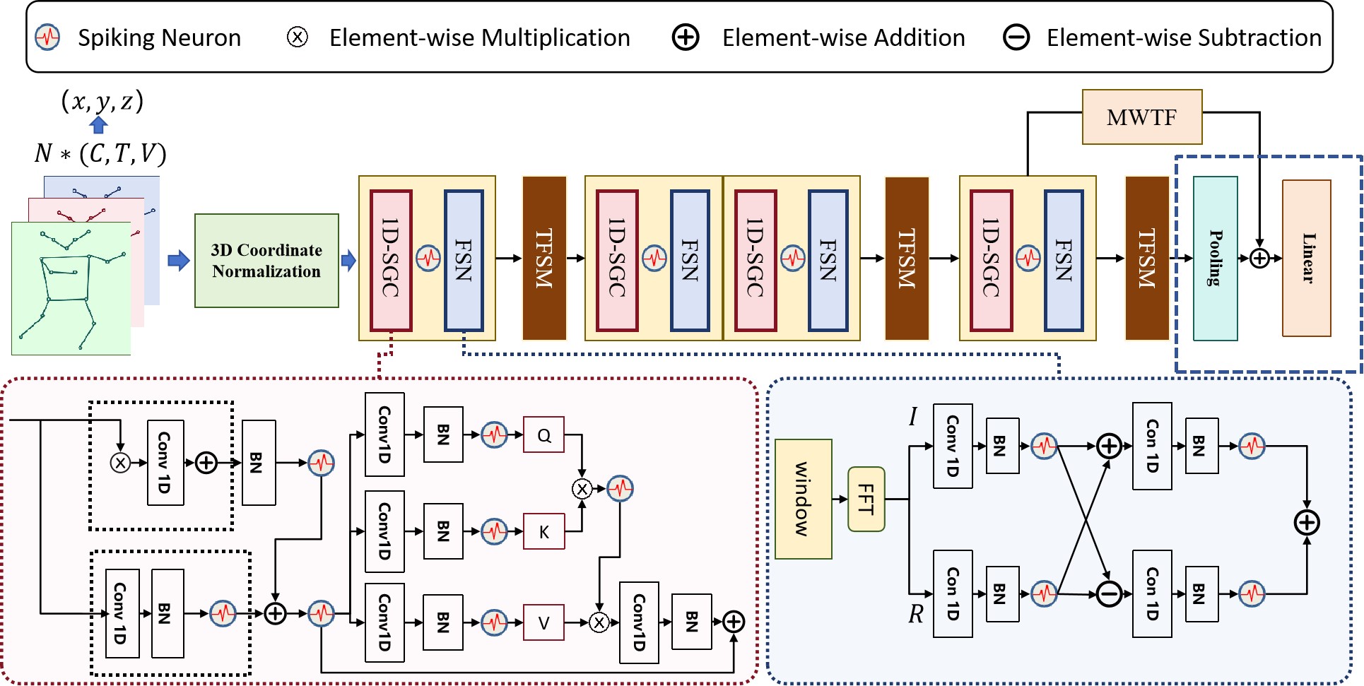
Figure 1: The overview of the proposed method.

Spiking Neural Networks

SNNs offer an energy-efficient alternative to traditional neural networks, inspired by biological neural networks(Neftci, Mostafa, and Zenke 2019). SNNs can be implemented through two primary design approaches: ANN-to-SNN conversion(Ding et al. 2021; Ho and Chang 2021) and direct training using specialized algorithms like STDP(Caporale and Dan 2008)and surrogate gradient methods(Neftci, Mostafa, and Zenke 2019). The fundamental units of SNNs are spiking neurons, with the Leaky Integrate-and-Fire (LIF) neuron being particularly notable for its simplicity and biological plausibility(Teeter et al. 2018). The details can be found in the Appendix. Existing SNN networks are often designed based on the ANN framework and applied to various fields(Cao, Chen, and Khosla 2015; Pedretti et al. 2020; Cai et al. 2024). Additionally, several spiking Transformers have been proposed for RGB image classification and event camera action recognition(Zhou et al. 2022; Yao et al. 2024b, a). They add a temporal dimension to static data and use spike-form features for feature transmission. The current SGN network(Zheng, Xia, and Liang 2024) for skeleton-based action recognition treats skeletal sequences as static data and introduces an extra spiking timestep dimension. This approach increases the temporal dimension, adding storage and computational costs during model training. Moreover, these methods overlook the discrete and non-periodic nature of spike-form features, using average pooling to average the spiking timestep dimension before classification.

Signal Processing in Deep Learning

Signal processing techniques are essential in various neural network architectures. In CNNs, FFT and Wavelet Transform(WT) enhance feature extraction for tasks such as image compression(Li et al. 2020). RNNs use FFT to analyze frequency components in sequential data, improving speech recognition(Jalayer, Orsenigo, and Vercellis 2021). GCNs leverage Fourier transforms to analyze graph signals for social network analysis(Yu and Qin 2020). Additionally, FFT and WT are effective in EEG signal processing, emotion analysis, and radar data interpretation(Xu et al. 2024; Henderson et al. 2023). Integrating these methods with deep learning and SNNs offers a robust framework for analyzing complex datasets. These insights inspire us to explore the potential of integrating signal analysis methods with SNNs for innovative applications in skeleton action recognition.

Method

We propose the Signal-SGN network, shown in Figure 1, which consists of four 1D-SGC and FSC layers and a linear classification head. We insert the TFSM module after three different levels of SGN-FSC layers to extract semantic features at various levels. Additionally, we embed the MWTF module before the linear classification head to fuse multi-level frequency features and enhance the model’s classification capability.

1D-SGC and FSC

In the backbone, the input is three-dimensional skeleton data $X\in\mathbb{R}^{C\times T\times V}$ where $C$ is the channel size, and each $T$ frame contains $V$ joint coordinates $(x,y,z)$. The coordinates can have positive and negative values since the $V$ joints are distributed across multiple quadrants in three-dimensional space. In GCN, floating-point operations can successfully handle this information. However, SNN uses rate coding and binarization, causing traditional SGN to be unable to process negative values, leading to information loss and impacting accuracy. To address this issue, we normalize the three-dimensional coordinates before inputting them into the network, converting $[x,y,z]$ to the range $[0,1]$.

$$a^{\prime}=\frac{a-a_{\min}}{a_{\max}-a_{\min}},\quad\text{where}\quad a\in{x,y,z}$$ (1)

In 1D-SGC, we draw inspiration from GCN and utilize graph convolution methods to incorporate topological information. By normalizing weights based on adjacency relationships, nodes can selectively aggregate the attributes of their neighbors. The human skeleton can be represented as a graph $G(V,E)$, where the joints form a set of $V$ vertices, and the bones represent the edges $E$. Edges can be represented as an adjacency matrix $A\in\mathbb{R}^{V\times V}$, where $A_{i,j}=1$ if joints $i$ and $j$ are physically connected, otherwise 0.

$$S=\widetilde{D}^{-\frac{1}{2}}\widetilde{A}\widetilde{D}^{\frac{1}{2}}$$ (2)

Here,$\widetilde{A}=A+I$is the adjacency matrix with added self-connections, $K$ is the number of graph convolution layers, and $\tilde{D}$ is the degree matrix of $\tilde{A}$. In our proposed method, we transform $X\in\mathbb{R}^{C\times T\times V}$ into $X^{\prime}\in\mathbb{R}^{T\times C^{\prime}\times V}$, where $C^{\prime}$ represents the normalized three-dimensional coordinates. Subsequently, we apply one-dimensional convolution (Conv1d) and one-dimensional Batch Normalization(BN) along the $C^{\prime}$ dimension to extract features for each skeleton node within each time step, effectively aggregating features across the skeleton joints dimension.

$$G_{0}=\sum_{\mathrm{i}=0}^{\mathrm{n}}\mathrm{BN}\left[\operatorname{Conv1d}\left(X^{\prime}*S^{i}\right)\right]$$ (3)

Where, $S^{i}$ are several matrices decomposed from $S$, resulting in $G_{0}\in\mathbb{R}^{T\times C\times V}$.

$$G_{i}=SN\left(G_{0}\right)+SN\left(\mathrm{BN}\left(\operatorname{Conv1d}\left(G_{0}\right)\right)\right.$$ (4)

To fully utilize the spiking neural network’s capability to process temporal information, we use the inherent temporal dimension of the features as the time step for the spiking neural network and input the features into the spiking neurons (SN), resulting in the Algorithm 1 in the Appendix.

where $G_{i}(t)$ is a tensor of dimensions $C\times V$, representing the input current at each time step. The returned tensor $G_{i}(t)$ has the same dimensions as $G_{o}(t)$, indicating whether a spike was emitted at each time step. And we get $G_{O}\in\mathbb{R}^{T\times C\times V}$. Subsequent spiking neurons perform similar operations. Spiration from (Zhou et al. 2022), we introduce the spike self-attention mechanism after the graph convolution operation. The formula is as follows:

$$Q,K,V=SN(\mathrm{BN}(\operatorname{Conv}1\mathrm{~{}d}(G_{o}))$$ (5)

$$\operatorname{SSA}(G_{o})=SN\left(QK^{T}V*s\right)$$ (6)

where s is scaling factor to control the large value of the matrix multiplication result. The following formula can express the complete process of the 1D-SGC:

$$G=G_{o}+SN\left(\mathrm{BN}\left(\operatorname{Conv1d}\left(\operatorname{SSA}\left(G_{o}\right)\right)\right)\right)$$ (7)

The spiking form features are discrete aperiodic signals in the temporal and other dimensions, composed of 0s and 1s. We design the FSC to capture frequency domain features, and the specific process is as follows. It is well known that for discrete aperiodic signals, it is necessary to design corresponding window functions to extract their frequency domain information. The design of the window function reduces the spectral leakage and improves the accuracy of frequency domain analysis. Based on this idea, we design window functions for the input features in the $V$ and $T$ dimensions.

$$w_{C}(c)=a_{0}-\left(1-a_{0}\right)*\cos\left(\frac{2\pi c}{C-1}\right),0\leq c\leq C-1$$ (8)

$$w_{V}(v)=a_{1}-\left(1-a_{1}\right)*\cos\left(\frac{2\pi v}{V-1}\right),0\leq v\leq V-1$$ (9)

$$F_{0}=G\cdot w_{C}(c)\cdot w_{V}(c),\quad F_{0}\in\mathbb{R}^{T\times C\times V}$$ (10)

We apply a 2D FFT on the $V$ and $T$ dimensions to transform the features from the temporal domain to the frequency domain.

$$F_{i}=\sum_{c=0}^{C-1}\sum_{v=0}^{V-1}F_{0}e^{-j2\pi\left(\frac{kc}{C}+\frac{mv}{V}\right)}=F_{i}^{R}+jF_{i}^{I}$$ (11)

Where $F_{i},\quad F_{i}^{R},\quad F_{i}^{I}\in\mathbb{R}^{T\times K\times M}$ represent the complex output, its real and imaginary parts, respectively. Real and imaginary parts represent the amplitude and phase information of the spike-form feature. We design a spiking complex convolution that processes and integrates the real and imaginary parts separately. The formula is as follows:

$$F_{i}^{1(2)}=SN\left[\left(\operatorname{BN}\left(\operatorname{Conv}1\mathrm{~{}d}\left(F_{i}^{R}\right)\right)\pm\left(\operatorname{BN}\left(\operatorname{Conv}1\mathrm{~{}d}\left(F_{i}^{l}\right)\right)\right]\right.\right.$$ (12)

$$F_{o}= \ SN\left(\mathrm{BN}\left(\operatorname{Conv1d}\left(F_{i}^{1}-F_{i}^{2}\right)\right)\right)$$ (13)

$$\ +SN\left(\mathrm{BN}\left(\operatorname{Conv1d}\left(F_{i}^{1}+F_{i}^{2}\right)\right)\right)$$

A complete 1D-SGC-FSC process can be written as

$$X_{l}=G_{l}+F_{l}+\operatorname{res}\left(G_{l-1}\right)$$ (14)

where $l$ represents the layer level, and $res$ denotes a residual network.

Multi-scale Wavelet Transform Feature Fusion Module

As previously mentioned, spiking neural networks transmit information through spikes. We use DWT to fully extract high-frequency and low-frequency components in the time domain to utilise the temporal dimension characteristics.

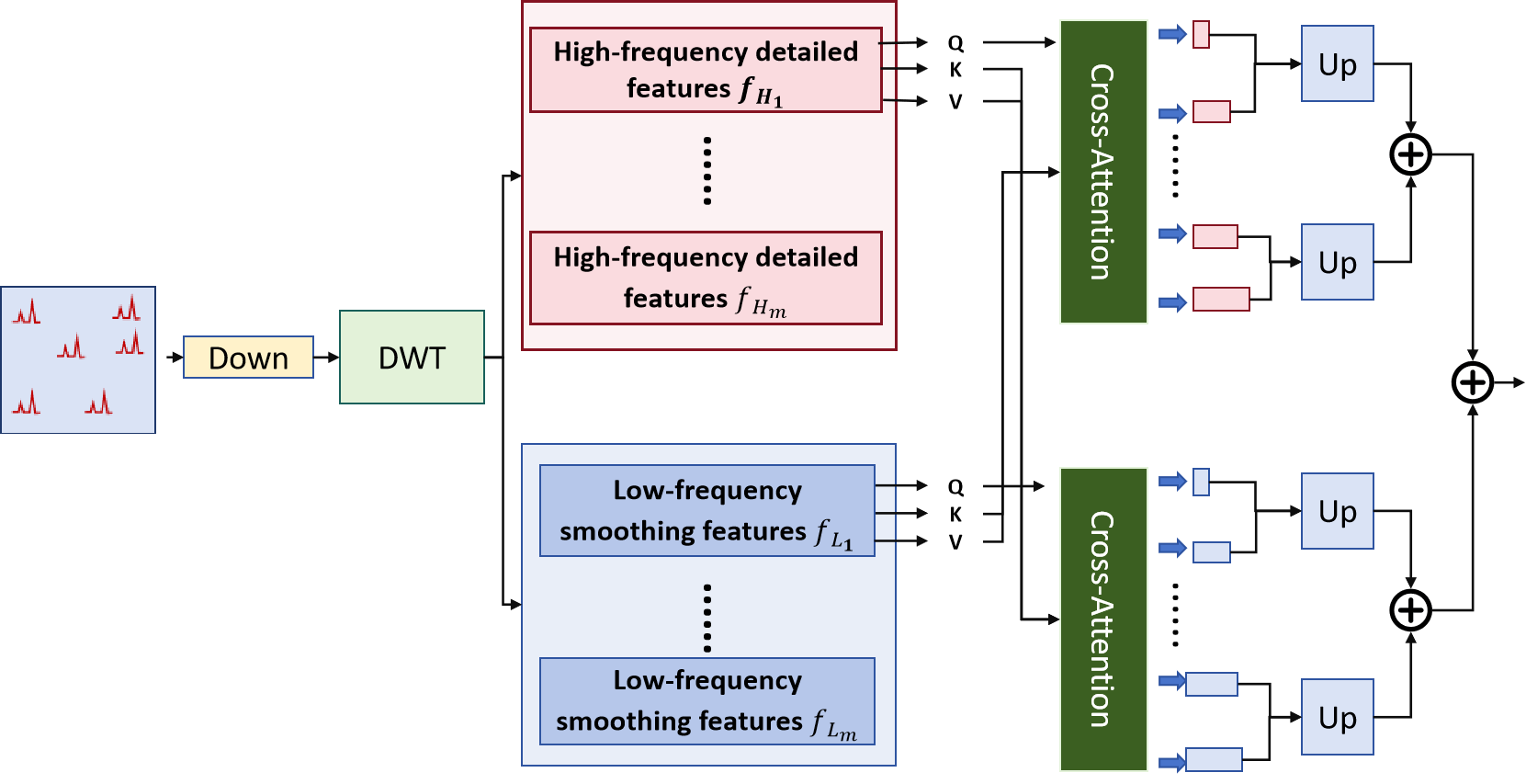
Figure 2: The Multi-scale Wavelet Transform Feature Fusion Module

We first downsample the spiking-form features

$$X_{\text{down}}=\operatorname{Down}\left(X_{4}\right),\quad X_{\text{down}}\in\mathbb{R}^{T\times C\times k}$$ (15)

We base our filter coefficients on Legendre polynomials (Yalçinbaş, Sezer, and Sorkun 2009).The Legendre polynomials $P_{k}(x)$ are a set of orthogonal polynomials defined on the interval $[-1,1]$. They satisfy the following recurrence relation:

$$P_{0}(x)=1$$ (16)

$$P_{1}(x)=x$$ (17)

$$(k+1)P_{k+1}(x)=(2k+1)xP_{k}(x)-kP_{k-1}(x)\text{ for }k\geq 1$$ (18)

To define the Legendre polynomials on the interval $[0,1]$, we apply a linear transformation $u=2x-1$, where $x\in[0,1]$. Thus, we have the equation of $P_{k}(2x-1)$. Specifically, for each $k$, we need to construct the corresponding low-frequency and high-frequency filters. Construction of Filter Matrices low-frequency filter $H_{0}$, high-frequency filter $H_{1}$, low-frequency detail filter $G_{0}$ and high-frequency detail filter$G_{1}$ is as follow:

$$H_{0}[k,t]=\sqrt{2k+1}\cdot P_{k}(u)$$ (19)

$$H_{1}[k,t]=\sqrt{2k+1}\cdot P_{k}(2u+1)$$ (20)

$$G_{0}[k,t]=\sqrt{2}\cdot\sqrt{2k+1}\cdot P_{k}(u)$$ (21)

$$G_{1}[k,t]=\sqrt{2}\cdot\sqrt{2k+1}\cdot P_{k}(2u+1)$$ (22)

where $u=2\left(\frac{t}{T}\right)-1$,$t$ denotes the sample point, and $T$ denotes the total number of samples. We check whether the temporal dimension of the feature is a power of two.If not, look for the power of 2 that is closest to its time dimension. We expand the feature $x$ to the length $n_{l}$ by padding the first $n_{l}-T$ value of the feature.

$$n_{s}=\left\lfloor\log_{2}(T)\right\rfloor$$ (23)

$$n_{l}=2^{\left\lceil\log_{2}(T)\right\rceil}$$ (24)

$$X_{\text{extra}}=X_{\text{down}}[0:(nl-T),:,:]$$ (25)

$$X_{\text{extended }}=\operatorname{concat}(X_{\text{down}},X_{\text{extra}},\text{ axis }=1)$$ (26)

We split the extended feature into even and odd indexed parts. Then, we concatenate the even and odd parts to form a new feature. Next, we apply the filter matrices $H_{0},H_{1},G_{0},G_{1}$ to decompose the feature. This process is iterated until reaching the predetermined number of layers $n_{s}$. The entire decomposition process can be represented in Algorithm 2 in the Appendix. We apply a cross-attention mechanism to each pair’s detail coefficients $D_{j}$ and $S_{j}$. The cross-attention operation can be mathematically represented as follows:

$$D_{j}^{out}=\operatorname{softmax}\left(\left(W_{Q}D_{j}\right)\left(W_{K}D_{j}\right)^{T}\right)W_{V}S_{j}$$ (27)

$$S_{j}^{out}=\operatorname{softmax}\left(\left(W_{Q}S_{j}\right)\left(W_{K}S_{j}\right)^{T}\right)W_{V}D_{j}$$ (28)

Each output pair $D_{j}^{out}$ and $S_{j}^{out}$ has dimensions $D_{j}^{out},S_{j}^{out}\in\mathbb{R}^{(T/2^{j})\times C\times k}$. The temporal dimension of each pair is halved compared to the previous pair. We use upsampling to match, aggregate multi-level outputs and have $X_{MLO}\in\mathbb{R}^{(T/2)\times C\times k}$. We fuse it with the output $X_{4}$ of the last layer of the backbone for classification.

$$y_{ic}=FC(\operatorname{pool}\left(X_{4}\right)+\alpha\operatorname{pool}\left(X_{MLO})\right)$$ (29)

$$L_{CE}=-\frac{1}{N}\sum_{i}\sum_{c}y_{ic}\log\left(p_{ic}\right)$$ (30)

where FC is fully connected layers, $\alpha$ is a learable parameter, $N$ is the number of samples in a training batch, $y_{ic}$ is the one-hot encoding of the $i$-th sample, and $p_{ic}$ is the predicted probability for class $c$.

Temporal-frequency Semantic Feature Extraction Module

The backbone network extracts the time domain and frequency domain features of human skeleton data in the form of spiking-form. However, spiking neural networks that convey information through spiking-form features often struggle to distinguish complex human skeletons. MWTF extracts the time-frequency semantics of spiking-form features and clusters the similar semantics of different actions to provide auxiliary supervision for enhancing the data discrimination ability of the main model.

It starts with a two-path network consisting of time-domain convolution and frequency-domain convolution.

$$f_{\text{temporal }}=\operatorname{Pool}\left(W_{\text{temporal }}X_{l}\right)$$ (31)

$$X_{\text{frequency}} =FFT\left(\operatorname{Pool}\left(SN\left(W_{\text{frequency}}X_{l}\right)\right)\right)$$ (32)

$$=X_{\text{frequency}}^{R}+jX_{\text{frequency}}^{l}$$

$$f_{\text{frequency }}=\operatorname{Pool}\left(\operatorname{SN}\left(W_{\text{frequency }}^{R}X_{\text{frequency }}^{R}\right)\right)$$ (33)

$$+\operatorname{Pool}\left(\operatorname{SN}\left(W_{\text{frequency }}^{l}X_{\text{frequency }}^{I}\right)\right)$$

$$Y_{\text{extract }}^{l}=f_{\text{temporal }}+\lambda f_{\text{spatial }}$$ (34)

Since the module is applied to the backbone network at levels $l=$1, 3, and 4, we designed a Multi-Level Feature Fusion Module to aggregate features of different sizes. This module captures both low-level and high-level semantics by adjusting its receptive field. The specific details are as follows:

$$f_{\text{dilaed }}(s)=\left(\mathbf{x}_{*_{d}}f\right)(s)=\sum_{i=0}^{k-1}f(i)\cdot\mathbf{x}_{s-d\cdot i}$$ (35)

Where x is the input sequence feature, f is the convolution kernel coefficient, is the dilation coefficient, is the size of the convolution kernel, and represents the direction of the dilated convolution

$$k_{c}=d\times(k-1)+1$$ (36)

$$X_{\text{fision }}=\left[\delta_{\text{temparal }},\delta_{\text{frequency}},\delta_{0}\right]$$ (37)

$$\delta_{\text{temporal }}=f_{\text{dilated }}\left(f_{\text{temporal }}\right)$$ (38)

$$\delta_{\text{frequency}}=f_{\text{atlated }}\left(f_{\text{frequency}}\right)$$ (39)

Where $X_{\text{fision }}$ represents the features obtained after the multi-level feature fusion module, $\delta_{\text{temparal }}$ represents the semantic features in the time domain, $\delta_{\text{frequency}}$ represents the semantic features in the frequency domain, and $\delta_{0}$ represents the offsets.The semantic tuple for each action category is formed by concatenating the time domain features, frequency domain features, and offsets.

$$\arg\min\sum_{P_{i}\in C}\operatorname{dis}\left(X_{\text{fusion}},P_{i}\right)$$ (40)

$P_{i}$ is the feature tuple representing the $i^{th}$ semantic category within the set of cluster centers $C$, and $\operatorname{dis}\left(X_{\text{fusion}},P_{i}\right)$ represents the semantic distance between $X_{\text{fusion}}$ and $P_{i}$. Cosine distance is used for candidate feature tuple matching

$$\operatorname{dis}(u,v)=\frac{uv^{T}}{\|u\|_{2}\|v\|_{2}}$$ (41)

where $u$ and $v$ are the two semantic tuples involved in the calculation. While finding the optimal matching semantic category, there exist other sub-optimal matching semantic categories that represent semantic categories similar to the target semantics. When updating the cluster centers, it is necessary not only to update the cluster center of the optimal matching result to ensure that it represents the most expressive feature tuple of the corresponding semantic, but also to update the cluster centers of sub-optimal similar semantics to increase the inter-class distance between similar semantics.

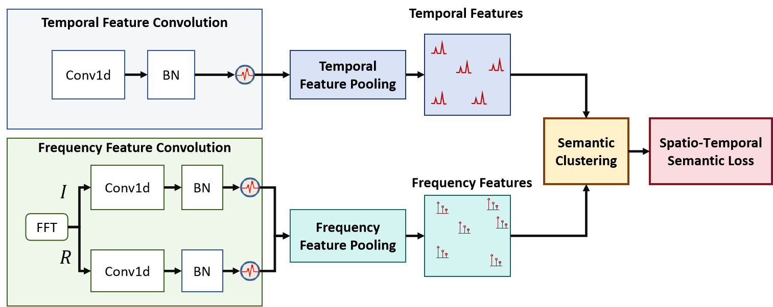
Figure 3: The Temporal-frequency Semantic Feature Extraction Module

$$P_{o}=P_{o}+\mu\frac{\operatorname{dis}\left(X_{\text{fusion}},P_{o}\right)}{n_{o}}$$ (42)

$$P_{e}=P_{e}+\beta\frac{\operatorname{dis}\left(X_{\text{fusion}},P_{e}\right)}{n_{e}}$$ (43)

The hyperparameters $\mu$ and $\beta$ represent the update step sizes for the best match and suboptimal match semantic category cluster centers, respectively. $P_{0}$ and $P_{e}$ represent the cluster centers for the best match and suboptimal match semantic categories, while $n_{o}$ and $n_{e}$. We use a multi-level MLP to fit the mapping relationships between low-level semantics and high-level semantics, as well as between high-level semantics and action categories, based on the semantic information obtained at different stages. Taking three different levels of semantic information as an example:

$$F_{\text{mid}}=MLP\left(F_{\text{low}}\right),F_{\text{high}}=MLP\left(F_{\text{mid}}\right),y_{i}=MLP\left(F_{\text{high}}\right)$$ (44)

Finally, we evaluate the model’s fitting degree to the semantic information through a contrastive loss function:

$$L_{SL}=\frac{1}{2N}\sum_{m=1}^{L}\omega\sum_{n=1}^{N}y_{i}\operatorname{dis}\left(F_{m},F_{m+1}\right)^{2}+$$ (45)

$$\left(1-y_{i}\right)\max\left(\omega_{\text{thre}}-\operatorname{dis}\left(F_{m},F_{m+1}\right),0\right)^{2}$$

$$L=L_{CE}+\omega L_{SL}$$ (46)

where $\omega$ is a hyperparameter.

Table 1: Comparison of experimental results under different module settings

Method	MWTF	TFSM	Param.	FLOPs/SOPs	Acc
			(M)	(G)	(%)
Ours	-	-	1.65	1.60/0.307	77.6
	✓	-	1.74	1.62/0.312	78.9
	-	✓	2.20	1.60/0.314	79.4
	✓	✓	2.28	1.62/0.329	80.5

Table 2: Comparative results on NTU RGB+D and NTU-RGB+D 120. We evaluate our model in terms of classification accuracy (%). Xs and Xv represent cross-subject and cross-view splits

Model	Param.	FLOPs	SOPs	Power	Accuracy (%)
(ANN/SNN)	(M)	(G)	(G)	(mJ)	Xs(60)	Xv(60)	Xs(120)	Xv(120)
Part-aware LSTM (Du, Wang, and Wang 2015)	-	-	-	-	62.93	70.27	25.5	26.3
Spatio-Temporal LSTM(Liu et al. 2016)	-	-	-	-	61.70	75.50	55.7	57.9
ST-GCN(Yan, Xiong, and Lin 2018)	2.11	2.56	-	11.78	81.5	88.3	70.7	73.2
2S-AGCN(Shi et al. 2019)	3.48	35.8	-	164.68	88.5	95.1	82.5	84.3
Shift-GCN(Cheng et al. 2020b)	-	10	-	46	90.7	96.5	85.3	86.6
MS-G3D(Liu et al. 2020)	3.19	67.63	-	311.09	91.5	96.2	86.9	88.4
CTR-GCN(Chen et al. 2021)	1.46	7.88	-	36.25	92.4	96.8	88.9	90.6
Spikformer (Zhou et al. 2022)ICLR 2023	4.78	24.07	1.69	2.17	73.9	80.1	61.7	63.7
Spike-driven Transformer (Yao et al. 2024a)NIPS2023	4.77	23.5	1.57	1.93	73.4	80.6	62.3	64.1
MK-SGN(Zheng, Xia, and Liang 2024)	2.17	7.84	0.68	0.614	78.5	85.6	67.8	69.5
Signal-SGN(Bone)	2.28	1.65	0.32	0.372	80.5	87.7	69.2	72.1
Signal-SGN(Bone+Joint)	2.28	3.31	0.64	0.644	82.5	89.2	71.3	74.2
Signal-SGN (4 ensemble)	2.28	6.62	1.28	1.288	86.1	93.1	75.3	77.9

Table 3: Comparative results on NW-UCLA.We evaluate our model in terms of classification accuracy (%).

Model	Param.	FLOPs	SOPs	Power	Acc
(ANN/SNN)	(M)	(G)	(G)	(mJ)	(%)
HBRNN-L(Du, Wang, and Wang 2015)	-	-	-	-	78.5
Ensemble TS-LSTM(Gao et al. 2022)	-	-	-	-	89.2
AGC-LSTM(Si et al. 2019)	-	10.9	-	50.14	93.2
DC-GCN+ADG(Cheng et al. 2020a)	2.48	3.6	-	16.56	95.3
CTR-GCN(Chen et al. 2021)	1.46	2.32	-	10.67	96.5
Spikformer (Zhou et al. 2022)ICLR 2023	4.78	8.55	0.513	0.673	85.4
Spike-driven Transformer (Yao et al. 2024a)NIPS2023	4.77	8.22	0.501	0.643	83.4
MK-SGN(Zheng, Xia, and Liang 2024)	2.17	3.66	0.165	0.207	92.3
Signal-SGN (Bone)	2.28	2.09	0.528	0.545	92.7
Signal-SGN (Bone+Joint)	2.28	4.18	1.06	1.11	93.13
Signal-SGN (4 ensemble)	2.28	8.36	2.12	2.23	95.9

Experiments

We evaluate the Signal-SGN model on three skeleton-based action recognition datasets: NTU-RGB+D(Shahroudy et al. 2016), NTU-RGB+D120(Liu et al. 2019), and NW-UCLA(Wang et al. 2014). Detailed hyperparameter design, the floating point operations (FLOPs), synaptic operations (SOPs), theoretical energy consumption calculations, and dataset descriptions can be found in the Appendix.

Ablation Studies

To analyze the effect of individual components of Signal-SGN, we examine the classification accuracy of different configurations of our model. All experimental ablation studies are conducted on NTU-RGB+D cross-subjects with bone data. During training and testing, sequences of the skeletons are batched together after being resized to 16 frames.

Backbone

We first verify the effectiveness of the backbone network described in Sec. 3.1, composed of four stacked 1D-SGN-FSN layers. As shown in Table 4 in the Appendix, we configure the input and output channels for each of these four layers. The network achieves a computational complexity of 1.60G FLOPs and 0.307G SOPs, demonstrating its efficiency in terms of computational resource usage. We use the cross-entropy loss function to calculate the network’s overall loss. Our results show an accuracy of 77.6% in Table 1, further demonstrating our backbone network’s effectiveness for skeleton-based action classification.

MWTF

We compare the classification accuracy before and after inserting the MWTF module, as shown in Table 1. The multi-level wavelet transform is determined by the temporal dimension of the input tensor, and we retain both high-frequency and low-frequency components of each level’s DWT for fusion. We find that after inserting this module, the model’s parameter count increases by only 0.09M, while the accuracy improves by 1.3%. Additionally, the floating-point operations increase by only 0.02 GFLOPs, and the SOPs increase by 0.005G, which is a very small cost compared to the accuracy improvement.

TFSM

We verify the impact of TFSM on the parameter count, finding that it increases the model’s parameters to 2.20M during training while improving the accuracy by 1.8%. Since TFSM is removed during the testing phase, the additional parameters do not affect the storage requirements for model deployment. Furthermore, we observe that the model’s FLOPs remain unchanged at 1.60G during the testing phase, and the fluctuations in SOPs are due to subtle changes in the spiking neuron firing rate.

Impact of Integrated Modules

After integrating both the MWTF and TFSM modules, the model’s parameter count during the training phase reaches 2.28M, while the floating-point operations during the testing phase remain at 1.62G, and the SOPs are 0.329G. The model’s accuracy improves to 80.5%, representing a 2.9% increase compared to the baseline backbone network. This demonstrates the effectiveness of our proposed modules and their low computational cost. Next, we compare our model with classical ANN models and state-of-the-art SNN models.

Comparison with the State-of-the-Art

Many state-of-the-art methods use multi-stream fusion. For fair comparison, we adopt the same four-stream fusion strategy: ”joint stream”, ”bone stream”, ”joint motion stream,” and ”bone motion stream”. Softmax scores from all streams are combined. Our Signal-SGN has three settings: 1-stream (joint stream), 2-stream (joint and bone streams), and 4-stream (all streams). We compare Signal-SGN with state-of-the-art methods on the three datasets to verify our method’s superiority, generality, and efficiency. We compare the experimental results with previous ANN and SNN methods. For SNN models(Zhou et al. 2022; Yao et al. 2024a) that have not been previously used on these datasets, we replicate the results using the same hierarchical architecture as MK-SGN(Zheng, Xia, and Liang 2024) for comparison. Additionally, to demonstrate the superiority of our method over state-of-the-art SNNs, we perform unimodal reproductions for (Zhou et al. 2022; Yao et al. 2024a). Table 2 and Table3 show the parameters of our proposed Signal-SGN model, including FLOPs, SOPs, and energy consumption for a single sample in both single-modal and multi-modal scenarios. They also show the test set accuracy in both single-modal and multi-modal scenarios.
In the NTU-RGB+D dataset, when using single-modality Bone data, our model not only surpasses state-of-the-art SNN models in accuracy but also significantly reduces floating-point operations and theoretical energy consumption compared to SNN models. Additionally, compared to classical ANN models, our model achieves higher accuracy than ST-GCN when integrating four modalities, which is quite rare for spiking neural networks. Notably, our model also requires fewer floating-point operations than the lightweight CTR-GCN and Shift-GCN models. In terms of theoretical energy consumption, our model reduces energy usage to less than 5% compared to GCN-based methods, which is highly significant in practical applications.
In the NW-UCLA dataset, we resize the skeleton sequences to 52 frames, consistent with the classic GCN model(Chen et al. 2021). Our model achieves an accuracy of 95.9%, which is only 0.6% lower than the classic CTR-GCN model while reducing theoretical energy consumption to one-fourth of CTR-GCN’s. This further demonstrates the efficiency and energy-saving capabilities of our model. Additionally, compared to the previous SGN model, the absence of an extra-temporal dimension $Times$ in our model reduces the FLOPs in single-modality testing scenarios, making it easier to train on standard devices.

Conclusion

We propose a novel Signal-SGN network designed to learn dynamic features in the time and frequency domains for skeleton-based action recognition. The core of our model consists of four stacked SGC-FSN layers that utilize spiking graph convolution to capture temporal features of skeletons converted into spike forms and employ FFT and spiking complex convolution to capture frequency domain features. Additionally, we introduce the innovative MWTF module, based on the concept of wavelet transform, to capture multi-resolution features that enhance classification performance. We also present the plug-and-play TFSM module, which leverages temporal-frequency domain semantics to further boost the model’s classification capabilities. Notably, our final model not only surpasses state-of-the-art SNNs in various aspects but also achieves accuracy comparable to classic ANN models while maintaining extremely low energy consumption.

Appendix

In the appendix, we first provide a detailed introduction of the dataset, followed by the hyperparameter settings and training details. Finally, we explain the calculation methods for firing rate, operations (OPs), and theoretical energy consumption.

Leaky Integrate-and-Fire (LIF) neuron

The differential equation describes the dynamics of the LIF neuron:

$$\tau_{m}\frac{dV(t)}{dt}=-V(t)+R\cdot I(t)$$

where $V(t)$ is the membrane potential at time $t$, $\tau_{m}$ is the membrane time constant representing the rate of potential decay, $R$ is the membrane resistance, and $I(t)$ is the input current at time $t$. When $V(t)$ reaches the threshold $V_{\text{th}}$, the neuron fires a spike and the membrane potential is reset to $V_{\text{reset}}$. This model captures the essential dynamics of neuron spiking behaviour, making it an effective tool for simulating SNNs.

Algorithm

Algorithm 1 Neuron Dynamics Simulation

1:  Input: $G\in\mathbb{R}^{T\times C\times V}$

2:  Parameters: $\tau$, $V_{\text{rest}}$, $R$, $V_{\text{th}}$

3:  Output: $G_{o}\in\mathbb{R}^{T\times C\times V}$

4:  Initialize $V(t)$ and $G_{o}$

5:  for $t=0$ to $T-1$ do

6:     $G_{i}(t)\leftarrow G[t,:,:]$

7:     $\tau\frac{dV(t)}{dt}\leftarrow-\left(V(t)-V_{\text{rest}}\right)+R\cdot G_{i}(t)$

8:     if $V(t)\geq V_{\text{th}}$ then

9:        $G_{o}[t,:,:]\leftarrow 1$

10:     else

11:        $G_{o}[t,:,:]\leftarrow 0$

12:     end if

13:  end for

14:  return $G_{o}\in\mathbb{R}^{T\times C\times V}$

Algorithm 2 Iterative Decomposition

1:  $X_{0}\leftarrow X_{\text{extended}}$

2:  for $j=1$ to $ns$ do

3:     $x_{\text{even}}^{(j)}\leftarrow x_{j}[::2,:,:]$

4:     $x_{\text{odd}}^{(j)}\leftarrow x_{j}[1::2,:,:]$

5:     $x_{a}^{(j)}\leftarrow\text{concat}(x_{\text{even}}^{(j)},x_{\text{odd}}^{(j)},\text{axis}=-1)$

6:     $D_{j}\leftarrow H_{0}\cdot x_{a}^{(j)}+H_{1}\cdot x_{a}^{(j)}$

7:     $S_{j}\leftarrow G_{0}\cdot x_{a}^{(j)}+G_{1}\cdot x_{a}^{(j)}$

8:     $x_{j+1}\leftarrow S_{j}$

9:  end for

10:  return $\{D_{j}\}_{j=0}^{ns-1}$ and $\{S_{j}\}_{j=0}^{ns}$

Datasets

NTU-RGB+D

NTU-RGB+D(Shahroudy et al. 2016) is a comprehensive dataset widely used in the field of skeleton-based action recognition. It contains 60 action classes and 56,000 video clips, making it a robust benchmark for evaluating action recognition models. The dataset provides detailed 3D skeleton data, RGB frames, depth maps, and infrared sequences, covering a diverse range of daily activities such as eating, walking, and interacting with objects. The skeleton data consists of 25 joints per subject, captured using the Microsoft Kinect v2 sensor, which allows for precise modeling of human movement. This dataset is particularly valuable for researchers because it includes a variety of subjects performing actions from multiple viewpoints, offering a rich source of information to develop and test models capable of understanding complex human behaviors.

NTU-RGB+D 120

NTU-RGB+D 120(Liu et al. 2019) is an extended version of the original NTU-RGB+D dataset, expanding the number of action classes from 60 to 120 and increasing the total number of video clips to over 114,000. This extension includes additional action categories that encompass more complex and subtle human interactions, such as ”taking a selfie” and ”writing on a board.” With 106 distinct subjects and more diverse camera angles, NTU-RGB+D 120 offers a more challenging and comprehensive benchmark for evaluating the scalability and generalization capabilities of action recognition models. The dataset retains the detailed skeleton tracking of its predecessor, providing 25 joints per person and ensuring that the data remains highly informative for developing models that require an in-depth understanding of spatial-temporal dynamics in human actions. As one of the largest skeleton-based action recognition datasets available, NTU-RGB+D 120 is instrumental in pushing the boundaries of research in this field.

NW-UCLA

The NW-UCLA dataset is a smaller but uniquely challenging dataset consisting of 10 action classes and 1,494 video clips. It is specifically designed to test the robustness of action recognition models against viewpoint variations. The dataset features actions like jumping, waving, and running, captured from multiple viewpoints using three Kinect cameras placed at different angles. Each action is performed by 10 subjects, offering diverse skeleton data with 20 joints per person. This setup mimics real-world scenarios where actions are observed from different perspectives, making it a critical dataset for evaluating how well models can maintain performance when faced with varying observational conditions. The NW-UCLA dataset is ideal for researchers aiming to enhance the adaptability and resilience of their models to changes in camera viewpoints, which is essential for applications in surveillance, human-computer interaction, and robotics.

Model Implementation and Configuration

The models used for conducting experiments are implemented using PyTorch, a popular deep learning framework known for its flexibility and efficiency, and SpikingJelly, a specialized library for spiking neural network research. Our implementation leverages the powerful features of these tools to effectively model and simulate the complex dynamics of spiking neural networks. The training process is conducted on four NVIDIA V100 GPUs, which provide the necessary computational power and memory to handle the large datasets and intricate computations involved in our experiments. This setup ensures that our models are trained efficiently, allowing us to explore the full potential of our approach in a scalable and robust manner.

Table 4: The parameter Settings of the Backbone

Level of Layers	Channel Size
	Input	Output
1	3	64
2	64	64
3	64	128
4	128	256

In this section, we also give the specific hyperparameters of the model and training settings in all experiments. Table 4. presents the parameter settings of the backbone network, detailing the input and output channel sizes across different layers to illustrate the model’s architectural configuration.

The various hyperparameter settings used in our experiments are also shown in the Table5.

Table 5: Hyper-parameter training settings of Signal-SGN.

Parameter	NTU-RGB+D	NTU-RGB+D	NW-UCLA
	60	120
Learning Rate	0.1/0.1	0.1/0.1	0.1/0.1
Decay rate	0.1/0.1	0.1/0.1	0.1/0.1
Batch Size	60	40	120
Time Steps	4	4	4
Training Epochs	64	64	64
Step	50	50	50
Dropout Rate	0.3	0.3	0.3
Weight Decay	1e-4	1e-4	1e-4
$\omega$	0.03	0.03	0.03
Optimizer	SGD	SGD	SGD

Power Consumption

We assume that multiply-and-accumulate (MAC) and accumulate (AC) operations are implemented on the 45 nm technology node with $E_{MAC}$ = 4.6 pJ and $E_{AC}$ = 0.9 pJ. We calculate the number of synaptic operations (SOP) of the spike before calculating the theoretical dynamic energy consumption by $\mathrm{SOPs}=fr\times T\times\mathrm{FLOPs}$, where $fr$ is firing rate, $T$ is the timesteps, and $\mathrm{FLOPs}$ is floating point operations per sample.

$$\begin{gathered}E_{\text{Signal-SGN }}=E_{EAC}\times\mathrm{FL}_{\mathrm{SNN}\text{ Conv }}^{1}+\\ E_{AC}\times\left[\left(\sum_{n=2}^{N}\mathrm{SOP}_{\mathrm{SNN}\text{ Conv }}^{n}+\sum_{m=1}^{M}\mathrm{SOP}_{\mathrm{SNN}\text{ FC }}^{m}\right.\right.\\ \left.\left.+\sum_{l=1}^{L}\mathrm{SOP}_{\mathrm{SNN}\text{ SSA }}^{l}+\sum_{f=1}^{F}\mathrm{SOP}_{\mathrm{SNN}\text{ FFT }}^{f}\right)+\mathrm{SOP}_{\mathrm{SNN}\text{ DWT }}\right]\end{gathered}$$ (47)

References

- Cai et al. (2024) Cai, S.; Zhang, R.; Zhang, M.; Wu, J.; and Li, H. 2024. EEG-based Auditory Attention Detection with Spiking Graph Convolutional Network. IEEE Transactions on Cognitive and Developmental Systems.
- Cao, Chen, and Khosla (2015) Cao, Y.; Chen, Y.; and Khosla, D. 2015. Spiking deep convolutional neural networks for energy-efficient object recognition. International Journal of Computer Vision, 113: 54–66.
- Caporale and Dan (2008) Caporale, N.; and Dan, Y. 2008. Spike timing–dependent plasticity: a Hebbian learning rule. Annu. Rev. Neurosci., 31(1): 25–46.
- Chen et al. (2021) Chen, Y.; Zhang, Z.; Yuan, C.; Li, B.; Deng, Y.; and Hu, W. 2021. Channel-wise topology refinement graph convolution for skeleton-based action recognition. In Proceedings of the IEEE/CVF international conference on computer vision, 13359–13368.
- Cheng et al. (2020a) Cheng, K.; Zhang, Y.; Cao, C.; Shi, L.; Cheng, J.; and Lu, H. 2020a. Decoupling gcn with dropgraph module for skeleton-based action recognition. In Computer Vision–ECCV 2020: 16th European Conference, Glasgow, UK, August 23–28, 2020, Proceedings, Part XXIV 16, 536–553. Springer.
- Cheng et al. (2020b) Cheng, K.; Zhang, Y.; He, X.; Chen, W.; Cheng, J.; and Lu, H. 2020b. Skeleton-based action recognition with shift graph convolutional network. In Proceedings of the IEEE/CVF conference on computer vision and pattern recognition, 183–192.
- Ding et al. (2021) Ding, J.; Yu, Z.; Tian, Y.; and Huang, T. 2021. Optimal ann-snn conversion for fast and accurate inference in deep spiking neural networks. arXiv preprint arXiv:2105.11654.
- Du, Fu, and Wang (2015) Du, Y.; Fu, Y.; and Wang, L. 2015. Skeleton based action recognition with convolutional neural network. In 2015 3rd IAPR Asian conference on pattern recognition (ACPR), 579–583. IEEE.
- Du, Wang, and Wang (2015) Du, Y.; Wang, W.; and Wang, L. 2015. Hierarchical recurrent neural network for skeleton based action recognition. In Proceedings of the IEEE conference on computer vision and pattern recognition, 1110–1118.
- Gao et al. (2022) Gao, Z.; Wang, P.; Lv, P.; Jiang, X.; Liu, Q.; Wang, P.; Xu, M.; and Li, W. 2022. Focal and global spatial-temporal transformer for skeleton-based action recognition. In Proceedings of the Asian Conference on Computer Vision, 382–398.
- Ghosh-Dastidar and Adeli (2009) Ghosh-Dastidar, S.; and Adeli, H. 2009. Spiking neural networks. International journal of neural systems, 19(04): 295–308.
- Henderson et al. (2023) Henderson, A.; Harbour, S.; Yakopcic, C.; Taha, T.; Brown, D.; Tieman, J.; and Hall, G. 2023. Spiking Neural Networks for LPI Radar Waveform Recognition with Neuromorphic Computing. In 2023 IEEE Radar Conference (RadarConf23), 1–6. IEEE.
- Ho and Chang (2021) Ho, N.-D.; and Chang, I.-J. 2021. TCL: an ANN-to-SNN conversion with trainable clipping layers. In 2021 58th ACM/IEEE Design Automation Conference (DAC), 793–798. IEEE.
- Jalayer, Orsenigo, and Vercellis (2021) Jalayer, M.; Orsenigo, C.; and Vercellis, C. 2021. Fault detection and diagnosis for rotating machinery: A model based on convolutional LSTM, Fast Fourier and continuous wavelet transforms. Computers in Industry, 125: 103378.
- Li et al. (2020) Li, S.; Xue, K.; Zhu, B.; Ding, C.; Gao, X.; Wei, D.; and Wan, T. 2020. Falcon: A fourier transform based approach for fast and secure convolutional neural network predictions. In Proceedings of the IEEE/CVF Conference on Computer Vision and Pattern Recognition, 8705–8714.
- Liu et al. (2019) Liu, J.; Shahroudy, A.; Perez, M.; Wang, G.; Duan, L.-Y.; and Kot, A. C. 2019. Ntu rgb+ d 120: A large-scale benchmark for 3d human activity understanding. IEEE transactions on pattern analysis and machine intelligence, 42(10): 2684–2701.
- Liu et al. (2016) Liu, J.; Shahroudy, A.; Xu, D.; and Wang, G. 2016. Spatio-temporal lstm with trust gates for 3d human action recognition. In Computer Vision–ECCV 2016: 14th European Conference, Amsterdam, The Netherlands, October 11-14, 2016, Proceedings, Part III 14, 816–833. Springer.
- Liu et al. (2020) Liu, Z.; Zhang, H.; Chen, Z.; Wang, Z.; and Ouyang, W. 2020. Disentangling and unifying graph convolutions for skeleton-based action recognition. In Proceedings of the IEEE/CVF conference on computer vision and pattern recognition, 143–152.
- Neftci, Mostafa, and Zenke (2019) Neftci, E. O.; Mostafa, H.; and Zenke, F. 2019. Surrogate gradient learning in spiking neural networks: Bringing the power of gradient-based optimization to spiking neural networks. IEEE Signal Processing Magazine, 36(6): 51–63.
- Pedretti et al. (2020) Pedretti, G.; Mannocci, P.; Hashemkhani, S.; Milo, V.; Melnic, O.; Chicca, E.; and Ielmini, D. 2020. A spiking recurrent neural network with phase-change memory neurons and synapses for the accelerated solution of constraint satisfaction problems. IEEE Journal on Exploratory Solid-State Computational Devices and Circuits, 6(1): 89–97.
- Plizzari, Cannici, and Matteucci (2021) Plizzari, C.; Cannici, M.; and Matteucci, M. 2021. Skeleton-based action recognition via spatial and temporal transformer networks. Computer Vision and Image Understanding, 208: 103219.
- Ren et al. (2024) Ren, B.; Liu, M.; Ding, R.; and Liu, H. 2024. A survey on 3d skeleton-based action recognition using learning method. Cyborg and Bionic Systems, 5: 0100.
- Shahroudy et al. (2016) Shahroudy, A.; Liu, J.; Ng, T.-T.; and Wang, G. 2016. Ntu rgb+ d: A large scale dataset for 3d human activity analysis. In Proceedings of the IEEE conference on computer vision and pattern recognition, 1010–1019.
- Shi et al. (2019) Shi, L.; Zhang, Y.; Cheng, J.; and Lu, H. 2019. Two-stream adaptive graph convolutional networks for skeleton-based action recognition. In Proceedings of the IEEE/CVF conference on computer vision and pattern recognition, 12026–12035.
- Si et al. (2019) Si, C.; Chen, W.; Wang, W.; Wang, L.; and Tan, T. 2019. An attention enhanced graph convolutional lstm network for skeleton-based action recognition. In Proceedings of the IEEE/CVF conference on computer vision and pattern recognition, 1227–1236.
- Teeter et al. (2018) Teeter, C.; Iyer, R.; Menon, V.; Gouwens, N.; Feng, D.; Berg, J.; Szafer, A.; Cain, N.; Zeng, H.; Hawrylycz, M.; et al. 2018. Generalized leaky integrate-and-fire models classify multiple neuron types. Nature communications, 9(1): 709.
- Wang et al. (2014) Wang, J.; Nie, X.; Xia, Y.; Wu, Y.; and Zhu, S.-C. 2014. Cross-view action modeling, learning and recognition. In Proceedings of the IEEE conference on computer vision and pattern recognition, 2649–2656.
- Xu et al. (2024) Xu, F.; Pan, D.; Zheng, H.; Ouyang, Y.; Jia, Z.; and Zeng, H. 2024. EESCN: A novel spiking neural network method for EEG-based emotion recognition. Computer methods and programs in biomedicine, 243: 107927.
- Yalçinbaş, Sezer, and Sorkun (2009) Yalçinbaş, S.; Sezer, M.; and Sorkun, H. H. 2009. Legendre polynomial solutions of high-order linear Fredholm integro-differential equations. Applied mathematics and computation, 210(2): 334–349.
- Yamazaki et al. (2022) Yamazaki, K.; Vo-Ho, V.-K.; Bulsara, D.; and Le, N. 2022. Spiking neural networks and their applications: A review. Brain Sciences, 12(7): 863.
- Yan, Xiong, and Lin (2018) Yan, S.; Xiong, Y.; and Lin, D. 2018. Spatial temporal graph convolutional networks for skeleton-based action recognition. In Proceedings of the AAAI conference on artificial intelligence, volume 32.
- Yao et al. (2024a) Yao, M.; Hu, J.; Hu, T.; Xu, Y.; Zhou, Z.; Tian, Y.; Xu, B.; and Li, G. 2024a. Spike-driven transformer v2: Meta spiking neural network architecture inspiring the design of next-generation neuromorphic chips. arXiv preprint arXiv:2404.03663.
- Yao et al. (2024b) Yao, M.; Hu, J.; Zhou, Z.; Yuan, L.; Tian, Y.; Xu, B.; and Li, G. 2024b. Spike-driven transformer. Advances in neural information processing systems, 36.
- Ye et al. (2020) Ye, F.; Pu, S.; Zhong, Q.; Li, C.; Xie, D.; and Tang, H. 2020. Dynamic gcn: Context-enriched topology learning for skeleton-based action recognition. In Proceedings of the 28th ACM international conference on multimedia, 55–63.
- Yu and Qin (2020) Yu, W.; and Qin, Z. 2020. Graph convolutional network for recommendation with low-pass collaborative filters. In International Conference on Machine Learning, 10936–10945. PMLR.
- Zheng, Xia, and Liang (2024) Zheng, N.; Xia, H.; and Liang, Z. 2024. MK-SGN: A Spiking Graph Convolutional Network with Multimodal Fusion and Knowledge Distillation for Skeleton-based Action Recognition. arXiv preprint arXiv:2404.10210.
- Zhou et al. (2022) Zhou, Z.; Zhu, Y.; He, C.; Wang, Y.; Yan, S.; Tian, Y.; and Yuan, L. 2022. Spikformer: When spiking neural network meets transformer. arXiv preprint arXiv:2209.15425.
- Zhu et al. (2022) Zhu, Z.; Peng, J.; Li, J.; Chen, L.; Yu, Q.; and Luo, S. 2022. Spiking graph convolutional networks. arXiv preprint arXiv:2205.02767.