Inflationary Dynamics in Einstein-Gauss-Bonnet Gravity Using New Slow-Roll Approximations considering Generalised Reheating

Abstract

The Cosmic Microwave Background (CMB) observations results reported by Planck satellite suggest a plateau characteristic in the flat potential of the inflaton field is favored to drive the Universe’s early acceleration. On that note, Power Law Plateau (PLP) potential has gained a lot of attention. In this study, we demonstrate that implementing this inflationary model in an Einstein-Gauss-Bonnet(EGB) gravity background makes the model compatible with observations while avoiding late-stage thermal inflation which is otherwise unavoidable in a standard scenario. More importantly, we have taken the PLP model as a case study to check the new slow-roll approximations method proposed in [1]. Then we take one step further to check the consequence of generalized reheating in this scenario. Thus opening a new promising window to study inflationary dynamics in EGB gravity.

I Introduction

The inflationary epoch, along with the standard hot Big Bang model, could resolute the understanding of the birth and evolution of our Universe to its current state [2], [3]). The first idea of inflation was proposed by Guth [4] and since then the inflationary epoch has gained tremendous attention and it has become an interdisciplinary study requiring both the fields of high energy physics and cosmology[5, 6, 7, 8, 9, 10]. CMB observations by the Planck and Wilkinson Microwave Anisotropy Probe(WMAP) missions have ruled out or strongly disfavoured most of the textbook models of inflation in the standard scenario[11, 12, 13]. Based on the current observation, it becomes evident that a plateau-like feature in the potential can satisfy the constraints imposed by CMB in the best possible manner. In a key study, Dimopoulos and Owen [14] presented the Power Law Plateau inflation (PLP) with plateau properties. However, in this theoretically justified model, one needs to incorporate a phase of thermal inflation to let it withstand the observational constraints while remaining in the conventional cold inflationary premise.

It was shown for the first time in [15] that, if one wants to develop the inflationary models under the UV complete string theory, PLP in the alternative theory of Randall-Sundrum brane-world[16, 17]can be compatible with the observation, along with it can circumvent the tighter constraints from string theory like swampland conjecture[18]. But, on the other hand, RS models suffer serious existential crises because of the continuous limitation on the scale provided by the braneworld theory[19]. It has been shown that in modified gravity the restriction on the inflationary models can be less stringent[20, 21, 22, 23, 24, 25, 26, 27, 28, 29, 30, 31, 32, 33, 34]. In other words, models which are disfavoured by observation in the standard cold inflationary can satisfy the observational constraints in the modified gravity. The addition of the Gauss-Bonnet component to the Einstein-Hilbert action does not affect the equations of motion as it is a total derivative. When EGB coupling $\xi(\phi)$ is combined with a function of the scalar field $\phi$, it becomes dynamically important. In string theory, the Gauss-Bonnet term serves as a quantum correction to the Einstein-Hilbert action. Numerous inflationary models have been studied in this context[35, 36, 37, 38, 39, 40, 41, 42, 43, 44, 44, 45, 46, 47, 48, 49, 50, 51, 52, 53, 54, 55, 56, 57, 58, 59, 60, 61, 62, 63, 64, 65, 66, 52, 67, 68, 69, 70, 71, 72], most widely studied EGB coupling is the inverse function of the scalar field[36, 37, 38, 39, 41, 49, 51, 54, 55]. However in this manuscript we will study different form of coupling which involves a $``\tanh"$ term[73]. In [1] the authors have presented a new kind of slow-roll approximations, which are found to be more accurate in comparison to the previous slow-roll approximations presented in[45]. As it has been already shown in [1] that new slow approximations are more accurate, we aim to do a case study of the new slow-roll approximations in the EGB scenario using the the PLP potential as a prototype. This serves the primary objective of this exercise. More importantly, we extend the study to accommodate the generalized reheating and review its effect in the effective EGB background. The standard cold inflationary scenario requires an epoch of reheating after the end of inflation to enter the radiation-dominated epoch and start the Big Bang Nucleosynthesis (BBN). Studying the reheating phase following the end of inflation is necessary for the conceptual development of inflationary model construction. We have studied reheating in this work and established the limits on the number of e-folding and reheating temperatures that are permitted by CMB data.

The paper is organized as follows: In section II, we will go over some of the fundamental critical features in the EGB framework. A theoretically well-motivated Power Law Plateau (PLP) potential for this study has been reviewed in section III. In section IV, the calculation of slow-roll parameters without any approximations, is reviewed. In section V, the new slow-roll approximations (SRA) as reported in the work [1] are reviewed. Finally, the analysis of the inflationary dynamics using the new SRA and the effect of generalized reheating has been reported in the sections VI and VII. Finally, we conclude in section VIII with our conclusions and future direction of work.

II Review of Einstein-Gauss Bonnet Gravity

The effective action of the Gauss-Bonnet term is described by the following action:

$$S=\int d^{4}x\sqrt{-g}\left[U_{0}R-\frac{1}{2}g^{\mu\nu}\partial_{\mu}\phi\partial_{\nu}\phi-V(\phi)-\frac{1}{2}\xi(\phi){\cal G}\right],$$ (2.1)

where $U_{0}>0$ is a constant, $V(\phi)$ and $\xi(\phi)$ are the potential and EGB coupling and differentiable functions. $R$ denotes the usual Ricci scalar. The EGB term is given by:

$$\mathcal{G}=R_{\mu\nu\rho\sigma}R^{\mu\nu\rho\sigma}-4R_{\mu\nu}R^{\mu\nu}+R^{2}.$$ (2.2)

Evolution of equations and dynamical system in Einstein-Gauss-Bonnet gravity can be written for a spatially flat FLRW metric [35, 45]as:

$$12H^{2}\left(U_{0}-2\xi_{,\phi}\psi H\right) = \psi^{2}+2V,$$ (2.3)

$$4\dot{H}\left(U_{0}-2\xi_{,\phi}\psi H\right) = {}-\psi^{2}+4H^{2}\left(\xi_{,\phi\phi}\psi^{2}+\xi_{,\phi}\dot{\psi}-H\xi_{,\phi}\psi\right),$$ (2.4)

$$\dot{\psi}+3H\psi = {}-V_{,\phi}-12H^{2}\xi_{,\phi}\left(\dot{H}+H^{2}\right),$$ (2.5)

where $H=\dot{a}/a$ denotes the Hubble parameter and $a(t)$ is the scale factor, dot stands for the time derivative here. The term $\psi=\dot{\phi}$ and $A_{,\phi}\equiv\frac{dA}{d\phi}$ (true for any function $A(\phi)$). By taking the time derivative of Eq. (2.3), we get

$$12H\dot{H}\left(U_{0}-2\xi_{,\phi}H\psi\right)-12H^{2}\left(\xi_{,\phi\phi}H{\psi}^{2}+\xi_{,\phi}\left[H\dot{\psi}+\dot{H}\psi\right]\right)-\psi\dot{\psi}-V_{,\phi}\psi=0.$$ (2.6)

Expressing $V_{,\phi}$ from (2.6):

$$V_{,\phi}=12H\dot{H}\left(\frac{U_{0}}{\psi}-2\xi_{,\phi}H\right)-12H^{2}\left(\xi_{,\phi\phi}H\psi+\xi_{,\phi}H\frac{\dot{\psi}}{\psi}+\xi_{,\phi}\dot{H}\right)-\dot{\psi}\,,$$ (2.7)

and substituting it to (2.5), we obtain that Eq. (2.4) is a result of Eqs. (2.3) and (2.5).

When $\xi_{,\phi}\neq 0$, then equations (2.4) and (2.5) do not form a dynamic system. Insted it is proficient to use of Eqs. (2.4) and (2.5) t form a dynamical system [74]:

$$\begin{split}\dot{\phi}=&\psi,\\ ~{}~{}~{}~{}~{}~{}~{}~{}~{}~{}~{}~{}~{}\dot{\psi}=&\frac{1}{B-2\xi_{,\phi}H\psi}\left\{3\left[3-4\,\xi_{,\phi\phi}H^{2}\right]\xi_{,\phi}H^{2}\psi^{2}+\left[3B+2\,\xi_{,\phi}V_{,\phi}-6U_{0}\right]H\psi-\frac{V^{2}}{U_{0}}X\right\},\\ \dot{H}=&\frac{1}{4\left(B-2\,\xi_{,\phi}H\psi\right)}\left\{\left(4\,\xi_{,\phi\phi}H^{2}-1\right)\psi^{2}-16\xi_{,\phi}H^{3}\psi-4\frac{V^{2}}{U_{0}^{2}}\,\xi_{,\phi}H^{2}X\right\},\end{split}$$ (2.8)

where

$$B=12\xi_{,\phi}^{2}H^{4}+U_{0},\qquad X=\frac{U_{0}^{2}}{V^{2}}\left(12\xi_{,\phi}H^{4}+V_{,\phi}\right).$$ (2.9)

Substituting $\dot{\psi}$ defined by Eq. (2.5) into Eq. (2.6), we get the third equation of system (2.8). So, this equation is a consequence of Eqs. (2.3) and (2.5).

As usual for inflationary model construction, the e-folding number $N=\ln(a/a_{e})$, where $a_{e}$ is a constant, is considered as a measure of time during inflation.

Using the relation ${d}/{dt}=H\,{d}/{dN}$ and introducing $\chi=\psi/H$, one can write system (2.8) as follows:

$$\begin{split}\frac{d\phi}{dN}=&\,\chi,\\ \frac{d\chi}{dN}=&\,\frac{1}{Q\left(B-2\xi_{,\phi}Q\chi\right)}\left\{3\left[3-4\xi_{,\phi\phi}Q\right]\xi_{,\phi}Q^{2}\chi^{2}+\left[3B+2\xi_{,\phi}V_{,\phi}-6U_{0}\right]Q\chi-\frac{V^{2}}{U_{0}}X\right\}\\ &{}-\frac{\chi}{2Q}\frac{dQ}{dN},\\ \frac{dQ}{dN}=&\,\frac{Q}{2\left(B-2\xi_{,\phi}Q\chi\right)}\left\{\left(4\xi_{,\phi\phi}Q-1\right)\chi^{2}-16\xi_{,\phi}Q\chi-4\frac{V^{2}}{U_{0}^{2}}\xi_{,\phi}X\right\},\end{split}$$ (2.10)

where $Q\equiv H^{2}$.

Equation (2.3) can be presented in the following form

$$24\xi_{,\phi}\chi Q^{2}+\left(\chi^{2}-12U_{0}\right)Q+2V=0.$$ (2.11)

and has solutions:

$$Q_{\pm}=\frac{12U_{0}-\chi^{2}\pm\sqrt{\left(12U_{0}-\chi^{2}\right)^{2}-192V\xi_{,\phi}\chi}}{48\xi_{,\phi}\chi},$$ (2.12)

if $\xi_{,\phi}\chi\neq 0$. In the opposite case, the unique solution exists

$$Q_{0}=\frac{2V}{12U_{0}-\chi^{2}}\,.$$ (2.13)

Equation (2.11) restricts the set of initial conditions of system (2.10).

Equations (2.4) and (2.5) can be transformed to the following equations:

$$2\frac{dQ}{dN}\left(U_{0}-2\xi_{,\phi}\chi Q\right)={}-Q\chi^{2}+4Q\left(\xi_{,\phi\phi}Q\chi^{2}+\xi_{,\phi}\left(\frac{\chi}{2}\frac{dQ}{dN}+Q\frac{d\chi}{dN}\right)-\xi_{,\phi}Q\chi\right),$$ (2.14)

$$\frac{\chi}{2}\,\frac{dQ}{dN}+Q\,\frac{d\chi}{dN}+3Q\,\chi={}-V_{,\phi}-6Q\,\xi_{,\phi}\left(\frac{dQ}{dN}+2Q\right).$$ (2.15)

III Reviewing PLP inflation

Beyond Poincare symmetry, supersymmetry is the last type of space-time symmetrisation permitted by the Coleman-Mandula no-go theorem[75]. According to [14], with this assumption, a superpotential may be expressed as:

$$W=\frac{S(\phi_{1}-\phi_{2})}{2m}~{},$$ (3.16)

where, $S,\phi_{1},\phi_{2}$ are the chiral superfields and $m$ is the associated sub-Planckian energy scale. From this idea, one can get the potential of the form:

$$V{(\phi)}=V_{0}M_{P}^{4}\left(\frac{\phi^{n}}{\phi^{n}+m^{n}}\right)^{q}~{}.$$ (3.17)

Where $M_{P}$ signifies the Planck mass and the $\phi$ is the inflation field. $V_{0}$ is the dimensionless parameter that needs to be fixed by matching the amplitude of the scalar power spectrum at the pivot scale to $2.098\times 10^{-9}$. Two potential parameters $n$ and $q$ can vary from $1$ to $4$, this leads to the $16$ different cases. Eq. 3.17 is the inflationary potential, we are interested in our study. It is obvious to see that, if $m$ is super-Planckian, then this leads to just a large field $\phi^{m}$ model class. Thus, keeping $m\leq 1$ in the Planck unit is necessary, for simplicity in our calculation, we take $m=1$. However, the analyses we present in this manuscript can be easily extended to other smaller values of $m$. The standard case has been studied in [14] and it needed a phase of thermal inflation to make it viable from the observational point of view. Studying such models in modified gravity can alleviate the necessity of thermal inflation.

IV The slow-roll parameters without any approximation

Following Refs. [37, 35, 45, 76], we consider the slow-roll parameters:

$$\varepsilon_{1}={}-\frac{\dot{H}}{H^{2}}={}-\frac{d\ln(H)}{dN},\qquad\varepsilon_{i+1}=\frac{d\ln|\varepsilon_{i}|}{dN},\quad i\geqslant 1,$$ (4.18)

$$\delta_{1}=\frac{2}{U_{0}}\xi_{,\phi}H\psi=\frac{2}{U_{0}}\xi_{,\phi}H^{2}\chi,\qquad\delta_{i+1}=\frac{d\ln|\delta_{i}|}{dN},\quad i\geqslant 1.$$ (4.19)

It is easy to see that

$$\delta_{2}=\frac{\dot{\psi}}{H\psi}+\frac{\xi_{,\phi\phi}\psi}{H\xi_{,\phi}}-\varepsilon_{1}.$$ (4.20)

Using system (2.10), we obtain that the parameter $\epsilon_{1}(N)$ satisfies the following equation:

$$\varepsilon_{1}={}-\frac{1}{2Q}\frac{dQ}{dN}={}-\frac{1}{4\left(B-2\xi_{,\phi}Q\chi\right)}\left\{\left(4\xi_{,\phi\phi}Q-1\right)\chi^{2}-16\xi_{,\phi}Q\chi-4\frac{V^{2}}{U_{0}^{2}}\xi_{,\phi}X\right\}\,.$$ (4.21)

Dividing Eq. (2.4) on Eq. (2.3), we get another form of $\epsilon_{1}$:

$$\varepsilon_{1}=\frac{3}{\psi^{2}+2V}\left[\psi^{2}-4H^{2}\left(\xi_{,\phi\phi}\psi^{2}+\xi_{,\phi}\dot{\psi}-H\xi_{,\phi}\psi\right)\right].$$ (4.22)

Note that we do not use any approximation, so, these expressions for $\epsilon_{1}$ are exact.

It is useful, to rewrite evolution equations in terms of the slow-roll parameters. Equations (2.3) and (2.4) are equivalent to

$$12U_{0}H^{2}\left(1-\delta_{1}\right)=\psi^{2}+2V=H^{2}\chi^{2}+2V\,,$$ (4.23)

$$4U_{0}\dot{H}\left(1-\delta_{1}\right)={}-\psi^{2}+2U_{0}H^{2}\delta_{1}\left(\delta_{2}+\varepsilon_{1}-1\right).$$ (4.24)

From Eq. (4.24), it follows

$$\psi^{2}=2U_{0}H^{2}\left[2\varepsilon_{1}-\delta_{1}+\delta_{1}\left(\delta_{2}-\varepsilon_{1}\right)\right]$$ (4.25)

and

$$\chi^{2}=2U_{0}\left[2\varepsilon_{1}-\delta_{1}+\delta_{1}\left(\delta_{2}-\varepsilon_{1}\right)\right]\,.$$ (4.26)

The spectral index $n_{s}$ and the tensor-to-scalar ratio $r$ are connected with the slow-roll parameters as follows [37],

$$n_{s}=1-2\varepsilon_{1}-\frac{2\varepsilon_{1}\varepsilon_{2}-\delta_{1}\delta_{2}}{2\varepsilon_{1}-\delta_{1}}=1-2\varepsilon_{1}-\frac{d\ln(r)}{dN}=1+\frac{d}{dN}\ln\left(\frac{Q}{U_{0}r}\right),$$ (4.27)

$$r=8|2\varepsilon_{1}-\delta_{1}|.$$ (4.28)

From Eq. (4.26), it follows that

$$r=\left|\frac{U_{0}}{\xi_{,\phi}^{2}Q^{2}}\delta_{1}^{2}-8\delta_{1}\delta_{2}+8\delta_{1}\varepsilon_{1}\right|\,.$$

After this, we can find

$$A_{s}=\frac{Q}{\pi^{2}U_{0}\,r}\,.$$ (4.29)

Substituting expression (4.26) into Eq. (4.23), we get

$$V=U_{0}H^{2}\left[6-2\varepsilon_{1}-5\delta_{1}-\delta_{1}\left(\delta_{2}-\varepsilon_{1}\right)\right]\,.$$ (4.30)

Exact expression for $\frac{dQ}{dN}$ is

$$\frac{dQ}{dN}=\frac{Q}{2\,U_{0}\left(1-\delta_{1}\right)}\left({}-\chi^{2}+2\,U_{0}\delta_{1}\left(\delta_{2}+\varepsilon_{1}-1\right)\right).$$ (4.31)

V New slow-roll approximations

To examine the stability of de Sitter solutions in model 2.1, an effective potential approch has been proposed in  [74] (see also, [45, 77]):

$$V_{eff}(\phi)={}-\frac{U_{0}^{2}}{V(\phi)}+\frac{1}{3}\xi(\phi).$$ (5.32)

V.1 New approximation I

Multiplying 4.23 to $Q$ and substituting $\psi$ in terms of the slow-roll parameter $\delta_{1}$, we obtain:

$$12\,{U_{0}}\,\left(1-{\delta_{1}}\right)Q^{2}-2VQ-\frac{\delta_{1}^{2}U_{0}^{2}}{4\,\xi^{2}_{,\phi}}=0\,.$$ (5.33)

Equation 5.33 always has a positive root $Q$ if $\delta_{1}<1$:

$$Q=\frac{V}{12\,U_{0}\,\left(1-\delta_{1}\right)}+\frac{\sqrt{{V}^{2}\xi_{,\phi}^{2}+3\,U_{0}^{3}\delta_{1}^{2}\left(1-\delta_{1}\right)}}{12\,U_{0}\,\left(1-\delta_{1}\right)|\xi_{,\phi}|}\,.$$ (5.34)

Let us assume that $\delta_{1}\ll 1$ and expand the obtained expression to series with respect to the slow-roll parameter $\delta_{1}$:

$$Q\approx{\frac{V}{6\,U_{0}}}+{\frac{V}{6\,U_{0}}}\delta_{1}+{\cal{O}}(\delta^{2}_{1})\,.$$ (5.35)

We construct slow-roll approximations with

$$Q\simeq\frac{V}{6\,U_{0}}\left(1+\delta_{1}\right)=\frac{1}{6U_{0}^{2}}\left[U_{0}V+2V\xi_{,\phi}H\psi\right]\,.$$ (5.36)

To distinguish the standard slow-roll approximation, we do not neglect $\delta_{1}$, so we should obtain $\delta_{1}(\phi)$ to get $Q(\phi)$. To do it we use the following approximation of Eq. (2.4):

$$\dot{H}\simeq{}-\frac{\psi^{2}+4H^{3}\xi_{,\phi}\psi}{4U_{0}\left(1-\delta_{1}\right)}.$$ (5.37)

Using Eq. (4.19) and neglecting terms proportional to $\delta_{1}^{3}$, we rewrite (5.37) as follows

$$\dot{H}\simeq{}-\frac{\delta_{1}}{4(1-\delta_{1})}\left(\frac{U_{0}\delta_{1}}{4\xi_{,\phi}^{2}Q}+2Q\right)\simeq{}-\frac{Q\delta_{1}}{2}-\frac{U_{0}\delta_{1}^{2}}{16\xi_{,\phi}^{2}Q}-\frac{Q\delta_{1}^{2}}{2}\,.$$ (5.38)

We neglect terms proportional to $\ddot{\phi}$ and ${\dot{\phi}}^{2}$ in Eq. (2.5) and use Eq. (4.19) to get the following approximate equation:

$$\frac{3U_{0}\delta_{1}}{2\xi_{,\phi}}={}-V_{,\phi}-12Q\xi_{,\phi}\left(\dot{H}+Q\right).$$ (5.39)

Substituting $Q$ and $\dot{H}$ from Eqs. (5.36) and (5.38) into Eq. 5.39 and neglecting terms, proportional to $\delta_{1}^{n}$, where $n\geqslant 2$, we get

$$\delta_{1}(\phi)={}-\frac{2\,V^{2}\xi_{,\phi}\,{V_{eff}}_{,\phi}}{V^{2}\xi_{,\phi}^{2}+3\,U_{0}^{3}}\,.$$ (5.40)

The knowledge of $\delta_{1}(\phi)$ allows us to obtain $Q(\phi)$ and $\chi(\phi)$. We obtain from Eq. (5.36) that

$$Q\simeq\frac{V}{6U_{0}}\left[1-\frac{2V^{2}\xi_{,\phi}{V_{eff}}_{,\phi}}{V^{2}\xi_{,\phi}^{2}+3U_{0}^{3}}\right]=\frac{V\left(9U_{0}^{3}-6U_{0}^{2}\xi_{,\phi}\,V_{,\phi}+\xi_{,\phi}^{2}V^{2}\right)}{18U_{0}\left(3U_{0}^{3}+\xi_{,\phi}^{2}V^{2}\right)}.$$ (5.41)

Therefore, Eq. (4.19) gives

$$\chi=\frac{U_{0}\delta_{1}}{2\xi_{,\phi}Q}\simeq{}-\frac{6U_{0}^{2}V{V_{eff}}_{,\phi}}{V^{2}\xi_{,\phi}^{2}+3U_{0}^{3}-2V^{2}\xi_{,\phi}{V_{eff}}_{,\phi}}={}-\frac{6U_{0}^{2}\left(3U_{0}^{2}V_{,\phi}+\xi_{,\phi}V^{2}\right)}{V\left(9U_{0}^{3}-6U_{0}^{2}\xi_{,\phi}V_{,\phi}+\xi_{,\phi}^{2}V^{2}\right)}\,,$$ (5.42)

hence,

$$\frac{dN}{d\phi}={}-\frac{V^{2}\xi_{,\phi}^{2}+3U_{0}^{3}-2V^{2}\xi_{,\phi}{V_{eff}}_{,\phi}}{6U_{0}^{2}V{V_{eff}}_{,\phi}}\,.$$ (5.43)

Let us get the slow-roll parameters as functions of $\phi$. Using Eq. (5.41), we get

$$\varepsilon_{1}(\phi)={}-\frac{1}{2}\frac{d\phi}{dN}\frac{d\ln(Q)}{d\phi}=\frac{3U_{0}^{2}\left(3U_{0}^{2}V_{,\phi}+\xi_{,\phi}V^{2}\right)}{V\left(9U_{0}^{3}-6U_{0}^{2}\xi_{,\phi}V_{,\phi}+\xi_{,\phi}^{2}V^{2}\right)}\,\frac{d\ln(Q)}{d\phi}\\$$ (5.44)

where

$$\frac{d\ln(Q)}{d\phi}=\frac{V_{,\phi}}{V}+\frac{2\left[\xi_{,\phi}\xi_{,\phi\phi}V^{2}+\xi_{,\phi}^{2}VV_{,\phi}-3U_{0}^{2}\xi_{,\phi\phi}V_{,\phi}-3U_{0}^{2}\xi_{,\phi}V_{,\phi\phi}\right]}{9U_{0}^{3}-6U_{0}^{2}\xi_{,\phi}V_{,\phi}+\xi_{,\phi}^{2}V^{2}}-\frac{2\xi_{,\phi}\xi_{,\phi\phi}V^{2}+2{\xi{,\phi}}^{2}VV_{,\phi}}{3U_{0}^{3}+\xi_{,\phi}^{2}V^{2}}.$$

Also, we get

$$\varepsilon_{2}(\phi)=\frac{U_{0}\delta_{1}}{2\xi_{,\phi}Q\varepsilon_{1}}{\varepsilon_{1}}_{,\phi}\,,\qquad\delta_{2}=\frac{U_{0}}{2Q\xi_{,\phi}}{\delta_{1}}_{,\phi}.$$ (5.45)

V.2 New approximation II

The second way to get $\delta_{1}(\phi)$ is the following. We neglect the term proportional to $\delta_{1}^{2}$ in Eq. (5.33) and get a nonzero solution:

$$Q=\frac{V}{6U_{0}(1-\delta_{1})}.$$ (5.46)

Using Eq. (4.19), we get

$$\frac{dQ}{dN}=\frac{V_{,\phi}\,\delta_{1}}{12\xi_{,\phi}Q(1-\delta_{1})}+\frac{V\delta_{1}\delta_{2}}{6U_{0}(1-\delta_{1})^{2}}=\frac{U_{0}\,V_{,\phi}\,\delta_{1}}{2\xi_{,\phi}V}+\frac{V\delta_{1}\delta_{2}}{6U_{0}(1-\delta_{1})^{2}}\,.$$ (5.47)

So,

$$\varepsilon_{1}={}-\frac{3\,U^{2}_{0}\,V_{,\phi}}{2V^{2}\xi_{,\phi}}\delta_{1}(1-\delta_{1})-\frac{\delta_{1}\delta_{2}}{2\,(1-\delta_{1})}\,.$$ (5.48)

From 4.20, we get

$$\dot{\psi}\approx\frac{U_{0}\delta_{1}}{2\xi_{\phi}}\left(\delta_{2}+\varepsilon_{1}-\frac{3U_{0}^{2}\xi_{,\phi\phi}\delta_{1}}{V\,\xi_{,\phi}^{2}}\right)\,.$$ (5.49)

Substituting formulae 5.46, 5.48, and 5.49 into 2.5, we get

$$\frac{U_{0}\delta_{1}}{2\xi_{\phi}}\left(\delta_{2}+\varepsilon_{1}-\frac{3U_{0}^{2}\xi_{,\phi\phi}\delta_{1}}{V\,\xi_{,\phi}^{2}}\right)+\frac{3U_{0}\delta_{1}}{2\xi_{,\phi}}+V_{,\phi}+\frac{12\xi_{,\phi}V^{2}\,V_{,\phi}}{36\,U_{0}^{2}(1-\delta_{1})^{2}}(1-\varepsilon_{1})=0$$ (5.50)

Multiplying this equation to $(1-\delta_{1})^{2}$ and supposing that any products of slow-roll parameters are negligible, we obtain the following linear equation in $\delta_{1}$:

$$\frac{9}{2}\left(\frac{U_{0}^{3}}{\xi_{,\phi}}-V_{,\phi}\,U_{0}^{2}\right){\delta_{1}}+3\,V_{,\phi}\,U_{0}^{2}+V^{2}\xi_{,\phi}=0.$$ (5.51)

Solving this equation, we get

$$\delta_{1}(\phi)={}-\frac{2\xi_{,\phi}\left(3U_{0}^{2}V_{,\phi}+V^{2}\xi_{,\phi}\right)}{9U_{0}^{2}\left(U_{0}-\xi_{,\phi}V_{,\phi}\right)}.$$ (5.52)

Now we can express $Q$, $\chi$, $N_{,\phi}\,$, and $\epsilon_{1}$ via $\phi$:

$$Q(\phi)\simeq\frac{V}{6U_{0}(1-\delta_{1}(\phi))}=\frac{3{U_{0}}V(U_{0}-\xi_{,\phi}V_{,\phi})}{2(9U_{0}^{3}-3U_{0}^{2}\xi_{,\phi}V_{,\phi}+2\xi_{,\phi}^{2}V^{2})},$$ (5.53)

$$\chi=\frac{U_{0}\delta_{1}}{2\xi_{,\phi}Q}\simeq{}-\frac{2(3U_{0}^{2}V_{,\phi}+\xi_{,\phi}V^{2})(9U_{0}^{3}-3U_{0}^{2}\xi_{,\phi}V_{,\phi}+2\xi_{,\phi}^{2}V^{2})}{27U_{0}^{2}V{(U_{0}-\xi_{,\phi}V_{,\phi})}^{2}},$$ (5.54)

$$\frac{dN}{d\phi}={}-\frac{27U_{0}^{2}V{\left(U_{0}-\xi_{,\phi}V_{,\phi}\right)}^{2}}{2\left(3U_{0}^{2}V_{,\phi}+\xi_{,\phi}V^{2}\right)\left(9U_{0}^{3}-3U_{0}^{2}\xi_{,\phi}V_{,\phi}+2\xi_{,\phi}^{2}V^{2}\right)},$$ (5.55)

$$\varepsilon_{1}(\phi)={}-\frac{1}{2}\frac{d\phi}{dN}\frac{d\ln(Q)}{d\phi}=\frac{\left(3U_{0}^{2}V_{,\phi}+\xi_{,\phi}V^{2}\right)\left(9U_{0}^{3}-3U_{0}^{2}\xi_{,\phi}V_{,\phi}+2\xi_{,\phi}^{2}V^{2}\right)}{27U_{0}^{2}V{\left(U_{0}-\xi_{,\phi}V_{,\phi}\right)}^{2}}\,\frac{d\ln(Q)}{d\phi}\,,$$ (5.56)

where

$$\frac{d\ln(Q)}{d\phi}=\frac{V_{,\phi}}{V}+\frac{\xi_{,\phi\phi}V_{,\phi}+\xi_{,\phi}V_{,\phi\phi}}{\xi_{,\phi}V_{,\phi}-U_{0}}+\frac{3U_{0}^{2}\xi_{,\phi\phi}V_{,\phi}+3U_{0}^{2}\xi_{,\phi}V_{,\phi\phi}-4\xi_{,\phi}\xi_{,\phi\phi}V^{2}-4\xi_{,\phi}^{2}VV_{,\phi}}{9U_{0}^{3}-3U_{0}^{2}\xi_{,\phi}V_{,\phi}+2\xi_{,\phi}^{2}V^{2}}\,.$$ (5.57)

VI Inflationary analysis

In the subsequent sections, we will provide the calculation of inflationary observable for PLP in the new slow roll approximations. For our analysis we choose the following form of the EGB coupling [78, 79]

$$\xi(\phi)=\frac{\xi_{1}}{V_{0}}\tanh\left(\xi_{2}(\phi)\right)$$ (6.58)

where, $\xi_{1}$, $\xi_{2}$ are the coupling constant and $V_{0}$ is the scale of inflation which we fix from scalar power spectrum. Substituting 3.17 and 6.58 in 5.32, we can derive the explicit form of the effective potential (keeping $M_{p}=1$):

$$V_{eff}(\phi)=\frac{-U_{0}^{2}\left(\frac{\phi^{n}}{\phi^{n}+m^{n}}\right)^{-q}}{V_{0}}+\frac{\xi_{1}\tanh\left(\xi_{2}\phi\right)}{3V_{0}}$$ (6.59)

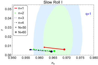
(a)

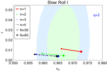
(b)

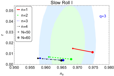
(c)

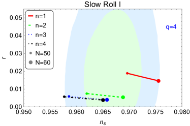
(d)

Figure 6.1: Plots of $r-n_{s}$ obtained by using Slow-Roll Approximation I for different values of $n$ and $q$ we vary N from $50$ to $60$. The red color line denotes the $n=1$, the dashed green line is for $n=2$, the dotted blue line is for $n=3$ and the black dot-dashed line signifies the $n=4$. Where the small and large dots of different color signify the $\text{N}=50$ and $\text{N}=60$ respectively. The light blue shaded area is for the $2-\sigma$ bounds, while the light green shaded area represents the $1-\sigma$ bounds on $n_{s}$ from Planck’18 [13]

VI.1 Inflationary Observables in Slow-Roll I

The knowledge of the slow-roll parameters as functions of $\phi$ allows us to get $n_{s}(\phi)$, $r(\phi)$, and $A_{s}(\phi)$ using formulae (4.27)–(4.29). Now, one can implement the above findings for the specific case of the PLP model. One can get the analytic expressions for the slow-roll parameters using the new approximation-I as given in A.1.

(a)

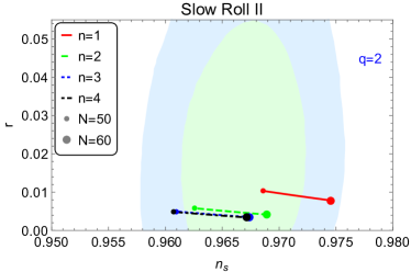
(b)

(c)

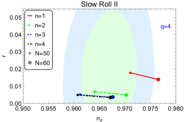
(d)

Figure 6.2: Plots of $r-n_{s}$ obtained by using Slow-Roll Approximation II for different values of $n$ and $q$ we vary N from $50$ top $60$. The red color line denotes the $n=1$, the dashed green line is for $n=2$, the dotted blue line is for $n=3$ and the black dot-dashed line signifies the $n=4$. Where the small and large dots of different colors signifies the $\text{N}=50$ and $\text{N}=60$ respectively. The light blue shaded area is for the $2-\sigma$ bounds, while the light green shaded area represents the $1-\sigma$ bounds on $n_{s}$ from Planck’18 [13]

Of course, the results look cumbersome, to say the least, but one should appreciate the fact that using these techniques, one can still get analytical solutions.

Now, we will discuss the PLP inflation in slow roll approximation I. To calculate the inflationary observables first we calculate the slow roll parameters, using 5.44 and 5.40 we compute $\varepsilon_{1},\delta_{1}$. It is then straightforward to obtain $\varepsilon_{2}$ and $\delta_{2}$ using 5.45. When studying inflation another important quantity is the number of e-folds $N$. Thus, from 5.43, one can write $N$ for a given $\phi$. To solve the 5.43 we followed the same prescription as mentioned in [1], and we have taken $N=60$ at the end of inflation whereas $N=0$ corresponds to the onset of the inflation.

We set the initial field value for solving 5.43 at the end of inflation which can be calculated from $\varepsilon_{1}=1$. It is difficult to solve the 5.43 analytically, we then employ the numerical techniques. Equipped with all the preliminary equations in hand, one can finally compute the scalar spectral index ($n_{s}$), the tensor to the scalar ratio ($r$), and the amplitude of scalar power spectrum ($A_{s}$) using 4.27,4.28 and 4.29 respectively. In our analysis we take $\xi_{1}=10$ and $\xi_{2}=0.4$, these values of the coupling parameters are chosen so that the constraints on $n_{s}$ and $r$ does not contradict with the current CMB bounds. Whereas, $V_{0}$ can be fixed by matching $A_{s}=2.09\times 10^{-9}$ at the pivot scale.

As we have previously mentioned $n$ and $q$ vary from $1$ to $4$, which results in the $16$ different class of potential. We have analyzed for all the possible combinations. In fig. 6.1 we present the results on the $r-n_{s}$ where Slow-Roll I approximation has been utilized. It is evident from fig. 6.1 that almost all the obtained values of $r$ and $n_{s}$ for combination of potential parameters $n$ and $q$ are well inside the constraints imposed by the Planck 18. Explicit numerical values of the inflationary observables can be found in table 6.1.

				$q=1$
	$n=1$		$n=2$		$n=3$		$n=4$
$N$	$r$	$n_{s}$	$r$	$n_{s}$	$r$	$n_{s}$	$r$	$n_{s}$
$50$	0.008604	0.961780	0.006397	0.957867	0.005970	0.9568	0.0059473	0.956564
$60$	0.006130	0.969175	0.0043752	0.96545	0.0059704	0.96450	0.00401488	0.96429
				$q=2$
	$n=1$		$n=2$		$n=3$		$n=4$
$N$	$r$	$n_{s}$	$r$	$n_{s}$	$r$	$n_{s}$	$r$	$n_{s}$
$50$	0.0114495	0.96616	0.006667	0.959685	0.0058103	0.957663	0.00580653	0.95712
$60$	0.008526	0.972857	0.004638	0.966922	0.00398821	0.965102	0.00393797	0.964671
				$q=3$
	$n=1$		$n=2$		$n=3$		$n=4$
$N$	$r$	$n_{s}$	$r$	$n_{s}$	$r$	$n_{s}$	$r$	$n_{s}$
$50$	0.0149482	0.968519	0.007059	0.960959	0.00581401	0.958181	0.00572878	0.957447
$60$	0.0114241	0.974752	0.004972	0.967989	0.00398117	0.965487	0.00389589	0.964897
				$q=4$
	$n=1$		$n=2$		$n=3$		$n=4$
$N$	$r$	$n_{s}$	$r$	$n_{s}$	$r$	$n_{s}$	$r$	$n_{s}$
$50$	0.0188761	0.969662	0.00750292	0.961960	0.0058097	0.958572	0.0056763	0.956782
$60$	0.0146428	0.975524	0.00533771	0.968838	0.003992	0.965786	0.00386787	0.965061

Table 6.1: Table for $r-n_{s}$ for different values of potential parameters in Slow-Roll I

VI.2 Inflationary Observables in Slow-Roll II

Using the obtained expressions of $\delta_{1}(\phi)$ and $\varepsilon_{1}(\phi)$ and Eq. 5.45, one can now calculate parameters $\varepsilon_{2}(\phi)$ and $\delta_{2}(\phi)$. One can again get the analytic expressions for the slow-roll parameters using the new approximation-II as given in A.2. After this, one can in the same spirit obtain $n_{s}(\phi)$, $r(\phi)$, and $A_{s}(\phi)$ using (4.27)–(4.29).

In this section we will discuss the PLP inflation in slow roll approximation II. We employ the same method to calculate the inflationary observables as we have employed in Slow Roll Approximation I. First we calculate the slow roll parameters ($\varepsilon_{1},\varepsilon_{2},\delta_{1},\delta_{2}$), using 5.56 and 5.52 we compute $\varepsilon_{1},\delta_{1}$. After this, it is straightforward to obtain $\varepsilon_{2}$ and $\delta_{2}$ using 5.45. Using 5.55 we calculate the number of e-folds $N$ by adopting the same technique as we did in the previous subsection(Slow-Roll Approximation I). Equipped with all the preliminaries we can finally compute the scalar spectral index ($n_{s}$), tensor to scalar ratio ($r$), and amplitude of scalar power spectrum ($A_{s}$) using 4.27,4.28 and 4.29 respectively. Here also, we take $\xi_{1}=10$ and $\xi_{2}=0.4$, these values of the coupling parameters are chosen so that the constraints on $n_{s}$ and $r$ does not contradict with the current CMB bounds. Whereas $V_{0}$ can be fixed by matching $A_{s}=2.09\times 10^{-9}$ at the pivot. As we have previously mentioned, $n$ and $q$ vary from $1$ to $4$, which results in the $16$ different class of potential. We have analyzed all the possible combinations. In fig. 6.2 we present the results on the $r-n_{s}$ where Slow-Roll I approximation has been utilized. It is evident from fig. 6.2 that almost all the obtained values of $r$ and $n_{s}$ for a combination of potential parameters $n$ and $q$ are well inside the constraints imposed by the Planck 18. Explicit numerical values of the inflationary observables can be found in table 6.2. A comparison between the two slow-roll approaches for a specific subclass of the PLP model is being given in the fig. 6.3.

				$q=1$
	$n=1$		$n=2$		$n=3$		$n=4$
$N$	$r$	$n_{s}$	$r$	$n_{s}$	$r$	$n_{s}$	$r$	$n_{s}$
$50$	0.00729363	0.96551	0.0052205	0.9611672	0.0049137	0.960799	0.00485738	0.96068
$60$	0.00535748	0.971735	0.0037563	0.96808	0.0034367	0.967247	0.00339305	0.967135
				$q=2$
	$n=1$		$n=2$		$n=3$		$n=4$
$N$	$r$	$n_{s}$	$r$	$n_{s}$	$r$	$n_{s}$	$r$	$n_{s}$
$50$	0.0103358	0.968584	0.00580519	0.962561	0.00497474	0.960935	0.00486187	0.960702
$60$	0.0078487	0.974514	0.00413578	0.968917	0.00348436	0.967372	0.00339693	0.967153
				$q=3$
	$n=1$		$n=2$		$n=3$		$n=4$
$N$	$r$	$n_{s}$	$r$	$n_{s}$	$r$	$n_{s}$	$r$	$n_{s}$
$50$	0.0138884	0.970306	0.00630019	0.963339	0.00503582	0.961067	0.00486645	0.960723
$60$	0.0107645	0.975965	0.0045256	0.969642	0.00353203	0.967494	0.00340085	0.967171
				$q=4$
	$n=1$		$n=2$		$n=3$		$n=4$
$N$	$r$	$n_{s}$	$r$	$n_{s}$	$r$	$n_{s}$	$r$	$n_{s}$
$50$	0.0178204	0.971075	0.00680496	0.964019	0.0050969	0.961195	0.00487111	0.960743
$60$	0.0139747	0.976535	0.00492388	0.970269	0.003579	0.967613	0.00340481	0.967189

Table 6.2: Table for $r-n_{s}$ for different values of potential parameters in Slow-Roll II

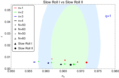
Figure 6.3: The comparison between the Slow Roll I and Slow Roll II for the PLP potential with $q=1$ and $n=1-4$. The legends are self-explanatory.

VII Reheating Parameters

After the end of the inflationary epoch, the universe goes into a super cold mode. In a standard cold inflationary scenario, the only degree of freedom that can survive after the inflation is the inflation field itself. However to repopulate the universe an era of reheating is required[80, 81, 82, 82], during which the inflaton field transfers its energy to other degrees of freedom, reviving the universe from a super-cooled state to a hot thermal bath of relativistic particles. The concept of reheating was first proposed in [81]. In the standard cold inflationary scenario, various methods of reheating have been suggested in the literature. One such method is perturbative decay, where the inflaton field reaches the bottom of its potential and begins to decay into other elementary particles[83, 84, 85, 86]. The resulting particles interact and reach equilibrium at a temperature known as the reheating temperature ($T_{re}$). More sophisticated methods include parametric resonance, which is a non-perturbative method, tachyonic instability[87], and preheating[88, 89]. The initial stage of reheating is often attributed to the preheating phase, which is more efficient than perturbative reheating because it involves exponential decay, generating a large number of particles.

However, it has been shown that the reheating era can be studied without delving into its actual dynamics[90]. Since there is no direct observational bound on the reheating temperature, analyzing this era indirectly can be extremely useful. This approach allows us to estimate the thermalization temperature using inflationary observables and can also serve as a new way to constrain different inflationary models. In addition to the reheating temperature ($T_{re}$) and the equation of state parameter ($\omega_{re}$), another crucial quantity is the duration of reheating ($N_{re}$). $N_{re}$ quantifies the expansion of the universe from the end of inflation to the end of the reheating era[90, 78, 79, 91].

Assuming, $w_{re}$ to be constant during the reheating epoch, the energy density of the universe at the end of inflation can be expressed in terms of scale factor through $\rho\propto a^{-3(1+w)}$, formulated as follows:

$$\frac{\rho_{end}}{\rho_{re}}=\left(\frac{a_{end}}{a_{re}}\right)^{-3(1+w_{re})},$$ (7.60)

The subscript $end$ signify the end of inflation, while $re$ stands for the end of the reheating period. Using the end of inflation condition($\epsilon=1$), we find $\rho_{end}=(3/2)V_{end}$ and substituting it in eq. 7.60, we find

$$N_{re}=\frac{1}{3(1+w_{re})}\ln\left(\frac{\rho_{end}}{\rho_{re}}\right)=\frac{1}{3(1+w_{re})}\ln\left(\frac{3}{2}\frac{V_{end}}{\rho_{re}}\right),$$ (7.61)

Also we know:

$$\rho_{re}=\frac{\pi^{2}}{30}g_{re}T_{re}^{4}.$$ (7.62)

Where, $g_{re}$ denotes the number of relativistic species at the end of reheating.

Using (7.61) and (7.62) and following [90, 92, 93], we can express $T_{re}$ and $N_{re}$ as :

$$N_{re}=\frac{1}{3(1+w_{re})}\ln\left(\frac{30\cdot\frac{3}{2}V_{end}}{\pi^{2}g_{re}T_{re}^{4}}\right)$$ (7.63)

Admitting that entropy is conserved from the reheating to today, one may write

$$T_{re}=T_{0}\left(\frac{a_{0}}{a_{re}}\right)\left(\frac{43}{11g_{re}}\right)^{\frac{1}{3}}=T_{0}\left(\frac{a_{0}}{a_{eq}}\right)e^{N_{RD}}\left(\frac{43}{11g_{re}}\right)^{\frac{1}{3}},$$ (7.64)

with $N_{RD}$ being the number of e-folds during radiation era, since $e^{-N_{RD}}\equiv a_{re}/a_{eq}$. The ratio $a_{0}/a_{eq}$ can be expressed as

$$\frac{a_{0}}{a_{eq}}=\frac{a_{0}H_{k}}{k}e^{-N_{k}}e^{-N_{re}}e^{-N_{RD}}\$$ (7.65)

We know for the modes at the horizon exit we can write, $k=a_{k}H_{k}$ and using the Eq. (7.63), (7.64) and (7.65), assuming $w_{re}\neq\frac{1}{3}$ and $g_{re}\approx 226$ (degrees of freedom in a supersymmetric model), we can derive the expression for $N_{re}$

$$N_{re}=\frac{4}{(1-3w_{re})}\left[61.488-\ln\left(\frac{V_{end}^{\frac{1}{4}}}{H_{k}}\right)-N_{k}\right]$$ (7.66)

Using Planck’s pivot ($k$) of order $0.05\;\mbox{Mpc}^{-1}$ we find $T_{re}$:

$$T_{re}=\left[\left(\frac{43}{11g_{re}}\right)^{\frac{1}{3}}\frac{a_{0}T_{0}}{k}H_{k}e^{-N_{k}}\left[\frac{3^{2}\cdot 5V_{end}}{\pi^{2}g_{re}}\right]^{-\frac{1}{3(1+w_{re})}}\right]^{\frac{3(1+w_{re})}{3w_{re}-1}}.$$ (7.67)

From 7.66 and 7.67 it is evident that to evaluate $N_{re}$ and $T_{re}$ first we require to calculate the $H_{k}$, $N_{k}$ (e-folds during the inflation) and $V_{end}$ (value of potential at the end of inflation). Utilizing the tensor-to-scalar ratio with scalar power spectrum we can write

$${H_{k}}=\sqrt{\frac{1}{2}\pi^{2}A_{s}r}.$$ (7.68)

Maintaining $A_{s}(k_{0})=2.0989\times 10^{-9}$, it is evident from Eq.(7.66) and (7.67) that both equations depend on $H_{k}$.

From Eq.(7.68), it’s clear that $H_{k}$ is a function of the tensor to scalar ratio ($r$). As we know from the CMB observation, tensor to scalar ratio has only upper bound. To precisely analyze the dynamics of reheating we need to express $H_{k}$ in terms of the spectral index ($n_{s}$). This can be done from the relation between $r,n_{s}$ and $N_{k}$[91, 78]. As mentioned in [90] varying $A_{s}$ with $n_{s}$ has negligible effect on the reheating. we keep $A_{s}(k_{0})=2.0989\times 10^{-9}$.

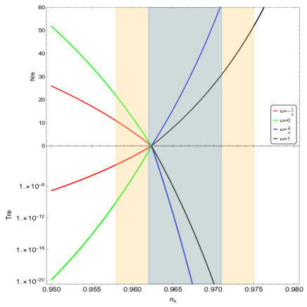
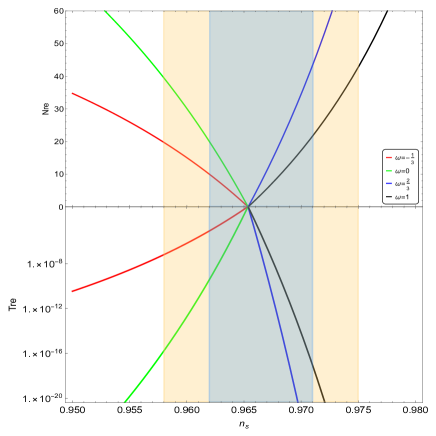
Figure 7.4: Plots illustrating $N_{re}$ and $T_{re}$ for different choices of $\omega_{re}$ are presented. Left Panel: The results for slow-roll approximation I is represented. Right Panel: The results for slow-roll approximation II is represented. The light yellow shaded area is for the $2-\sigma$ bounds, while the blue shaded area represents the $1-\sigma$ bounds on $n_{s}$ from Planck’18 [13]. Finally, the self-explanatory color coding for $w_{re}$ is given in the inset of the plots.

The variation of $N_{re}$ and $T_{re}$ for the PLP model with $n=2$ and $q=1$ for various values of $w_{re}$ is shown in Fig. 7.4. The convergence points on the $T_{re}$ and $N_{re}$ plots represent instantaneous reheating, with $N_{re}=0$. One can of course do this exercise for all the 16 combinations for this class of inflationary model. But the essence of the findings can be encapsulated in one of these figures such as fig. 7.4.

VIII Conclusions and Discussions

With future observations like CMB-S4 [94] and COrE [95] with promising prospects to measure the spectral tilt very precisely ($\Delta n_{s}\sim 0.002$), and with future possibilities to constrain the primordial tensor modes, a revisit to theoretically well-motivated models are in order. Not only that, the conceptual development in the modified gravity sector in the last few years has opened a window to study several interesting features to study. In the case of EGB gravity, new developments such as the new slow roll approximations methods as proposed in [1], beg a more detailed analysis. In this work, we had a threefold objective:

• Rescue a theoretically well-motivated model using a non-standard gravitational background of EGB gravity which we show can be done successfully.

• Implement the newly proposed idea of slow-roll approximation in the case of the PLP model and check the difference in predictivity depending on the approximation method.

• Finally, in the light of a more realistic case of generalized reheating, how the inflationary predictivity enlightens us on a model in the EGB background.

Thus, using this prescription, we have summarised a path to study inflationary dynamics in the EGB gravity. We have shown the class of PLP inflationary dynamics in the EGB background can successfully give observationally astute results even keeping the generalized reheating in mind.

A few more studies that we plan to conduct in the EGB inflationary the framework will be to see how the dynamics of Warm inflation get incorporated [96, 97]. Production of Primordial Black Holes and Gravitational Waves in case of warm inflationary dynamics [98, 99, 100, 101] in the EGB background, utilizing this new prescription could be a really interesting path to follow. The authors would like to come to these questions in future studies.

Appendix A Explicit Analytic Forms of Slow-Roll Parameters

A.1 New Slow Roll Approximation I

The slow-roll parameters in the case of slow-roll approximation I are given below:

$$\delta_{1}=-\frac{\text{{\hbox{\xi_1}}}\text{{\hbox{\xi_2}}}\text{sech}^{2}(\text{{\hbox{\xi_2}}}\phi)\left(\frac{\phi^{n}}{m^{n}+\phi^{n}}\right)^{2q}\left(3nqm^{n}\phi^{-n-1}\left(\frac{\phi^{n}}{m^{n}+\phi^{n}}\right)^{1-q}+4\text{{\hbox{\xi_1}}}\text{{\hbox{\xi_2}}}\text{sech}^{2}(\text{{\hbox{\xi_2}}}\phi)\right)}{6\left(\text{{\hbox{\xi_1}}}^{2}\text{{\hbox{\xi_2}}}^{2}\text{sech}^{4}(\text{{\hbox{\xi_2}}}\phi)\left(\frac{\phi^{n}}{m^{n}+\phi^{n}}\right)^{2q}+\frac{3}{8}\right)}$$

$$\delta_{2} = \Bigg{[}9\cosh^{4}\left(\xi_{2}\phi\right)\Bigg{(}-3nqm^{n}\cosh^{4}\left(\xi_{2}\phi\right)\left(m^{n}(nq-1)-(n+1)\phi^{n}\right)nq\phi+m^{n}\left(m^{n}+\phi^{n}\right)\cosh^{2}\left(\xi_{2}\phi\right)$$

$$\xi_{2}\left(3\sinh\left(2\xi_{2}\phi\right)-8\xi_{1}\left(\frac{\phi^{n}}{m^{n}+\phi^{n}}\right)^{q}\right)+8\xi_{1}\left(\frac{\phi^{n}}{m^{n}+\phi^{n}}\right)^{q}\bigg{(}\phi^{2}\left(m^{n}+\phi^{n}\right)^{2}\sinh\left(2\xi_{2}\phi\right)+nqm^{n}\left(\frac{\phi^{n}}{m^{n}+\phi^{n}}\right)^{q}$$

$$\xi_{1}\left(m^{n}(nq+1)+(n+1)\phi^{n}\right)\bigg{)}\xi_{2}^{2}-16n\xi_{1}^{2}\xi_{2}^{3}q\phi m^{n}\left(m^{n}+\phi^{n}\right)\tanh\left(\xi_{2}\phi\right)\left(\frac{\phi^{n}}{m^{n}+\phi^{n}}\right)^{2q}\Bigg{)}\Bigg{]}\Bigg{/}\Bigg{[}\phi\left(m^{n}+\phi^{n}\right)\times$$

$$\Bigg{(}8\xi_{1}^{2}\xi_{2}^{2}\left(\frac{\phi^{n}}{m^{n}+\phi^{n}}\right)^{2q}+3\cosh^{4}\left(\xi_{2}\phi\right)\Bigg{)}\Bigg{(}9\phi\left(m^{n}+\phi^{n}\right)\cosh^{4}\left(\xi_{2}\phi\right)-12n\xi_{1}\xi_{2}qm^{n}\cosh^{2}\left(\xi_{2}\phi\right)\left(\frac{\phi^{n}}{m^{n}+\phi^{n}}\right)^{q}$$

$$+8\xi_{1}^{2}\xi_{2}^{2}\phi\left(m^{n}+\phi^{n}\right)\left(\frac{\phi^{n}}{m^{n}+\phi^{n}}\right)^{2q}\Bigg{)}\Bigg{]}$$

$$\varepsilon_{1} = \Bigg{[}27\left(\frac{\phi^{n}}{m^{n}+\phi^{n}}\right)^{-2q}\left(\xi_{1}^{2}\xi_{2}^{2}\text{sech}^{4}\left(\xi_{2}\phi\right)\left(\frac{\phi^{n}}{m^{n}+\phi^{n}}\right)^{2q}+\frac{3}{8}\right)\Bigg{(}\xi_{1}\xi_{2}V_{0}\text{sech}^{2}\left(\xi_{2}\phi\right)\left(\frac{\phi^{n}}{m^{n}+\phi^{n}}\right)^{2q}$$ (1.1)

$$+\frac{3}{4}nqV_{0}m^{n}\phi^{-n-1}\left(\frac{\phi^{n}}{m^{n}+\phi^{n}}\right)^{q+1}\Bigg{)}\Bigg{(}\frac{qV_{0}\left(\frac{n\phi^{n-1}}{m^{n}+\phi^{n}}-\frac{n\phi^{2n-1}}{\left(m^{n}+\phi^{n}\right)^{2}}\right)\left(\frac{\phi^{n}}{m^{n}+\phi^{n}}\right)^{q-1}}{9\left(\xi_{1}^{2}\xi_{2}^{2}\text{sech}^{4}\left(\xi_{2}\phi\right)\left(\frac{\phi^{n}}{m^{n}+\phi^{n}}\right)^{2q}+\frac{3}{8}\right)}$$

$$\times\left(\xi_{1}^{2}\xi_{2}^{2}\text{sech}^{4}\left(\xi_{2}\phi\right)\left(\frac{\phi^{n}}{m^{n}+\phi^{n}}\right)^{2q}-\frac{1}{2}3n\xi_{1}\xi_{2}qm^{n}\phi^{-n-1}\text{sech}^{2}\left(\xi_{2}\phi\right)\left(\frac{\phi^{n}}{m^{n}+\phi^{n}}\right)^{q+1}+\frac{9}{8}\right)$$

$$-\frac{V_{0}\left(\frac{\phi^{n}}{m^{n}+\phi^{n}}\right)^{q}}{9\left(\xi_{1}^{2}\xi_{2}^{2}\text{sech}^{4}\left(\xi_{2}\phi\right)\left(\frac{\phi^{n}}{m^{n}+\phi^{n}}\right)^{2q}+\frac{3}{8}\right){}^{2}}\Bigg{(}\xi_{1}^{2}\xi_{2}^{2}\text{sech}^{4}\left(\xi_{2}\phi\right)\left(\frac{\phi^{n}}{m^{n}+\phi^{n}}\right)^{2q}-\frac{1}{2}3n\xi_{1}\xi_{2}qm^{n}\phi^{-n-1}\text{sech}^{2}\left(\xi_{2}\phi\right)\left(\frac{\phi^{n}}{m^{n}+\phi^{n}}\right)^{q+1}$$

$$+\frac{9}{8}\Bigg{)}\left(2\xi_{1}^{2}\xi_{2}^{2}q\left(\frac{n\phi^{n-1}}{m^{n}+\phi^{n}}-\frac{n\phi^{2n-1}}{\left(m^{n}+\phi^{n}\right)^{2}}\right)\text{sech}^{4}\left(\xi_{2}\phi\right)\left(\frac{\phi^{n}}{m^{n}+\phi^{n}}\right)^{2q-1}-4\xi_{1}^{2}\xi_{2}^{3}\tanh\left(\xi_{2}\phi\right)\text{sech}^{4}\left(\xi_{2}\phi\right)\left(\frac{\phi^{n}}{m^{n}+\phi^{n}}\right)^{2q}\right)$$

$$+\frac{\left(\frac{\phi^{n}}{m^{n}+\phi^{n}}\right)^{q}}{9\left(\xi_{1}^{2}\xi_{2}^{2}\text{sech}^{4}\left(\xi_{2}\phi\right)\left(\frac{\phi^{n}}{m^{n}+\phi^{n}}\right)^{2q}+\frac{3}{8}\right)}V_{0}\Bigg{(}\frac{1}{2}(-3)(-n-1)n\xi_{1}\xi_{2}qm^{n}\phi^{-n-2}\text{sech}^{2}\left(\xi_{2}\phi\right)\left(\frac{\phi^{n}}{m^{n}+\phi^{n}}\right)^{q+1}-$$

$$\frac{3}{2}n\xi_{1}\xi_{2}q(q+1)m^{n}\phi^{-n-1}\left(\frac{n\phi^{n-1}}{m^{n}+\phi^{n}}-\frac{n\phi^{2n-1}}{\left(m^{n}+\phi^{n}\right)^{2}}\right)\text{sech}^{2}\left(\xi_{2}\phi\right)\left(\frac{\phi^{n}}{m^{n}+\phi^{n}}\right)^{q}+2q\left(\frac{\phi^{n}}{m^{n}+\phi^{n}}\right)^{2q-1}$$

$$\xi_{1}^{2}\xi_{2}^{2}\left(\frac{n\phi^{n-1}}{m^{n}+\phi^{n}}-\frac{n\phi^{2n-1}}{\left(m^{n}+\phi^{n}\right)^{2}}\right)\text{sech}^{4}\left(\xi_{2}\phi\right)+3n\xi_{1}\xi_{2}^{2}qm^{n}\phi^{-n-1}\tanh\left(\xi_{2}\phi\right)\text{sech}^{2}\left(\xi_{2}\phi\right)\left(\frac{\phi^{n}}{m^{n}+\phi^{n}}\right)^{q+1}$$

$$-4\xi_{1}^{2}\xi_{2}^{3}\tanh\left(\xi_{2}\phi\right)\text{sech}^{4}\left(\xi_{2}\phi\right)\left(\frac{\phi^{n}}{m^{n}+\phi^{n}}\right)^{2q}\Bigg{)}\Bigg{)}\Bigg{]}\Bigg{/}$$

$$4V_{0}^{2}\left(\xi_{1}^{2}\xi_{2}^{2}\text{sech}^{4}\left(\xi_{2}\phi\right)\left(\frac{\phi^{n}}{m^{n}+\phi^{n}}\right)^{2q}-\frac{1}{2}3n\xi_{1}\xi_{2}qm^{n}\phi^{-n-1}\text{sech}^{2}\left(\xi_{2}\phi\right)\left(\frac{\phi^{n}}{m^{n}+\phi^{n}}\right)^{q+1}+\frac{9}{8}\right){}^{2}$$

$$\varepsilon_{2} = \bigg{[}3\left(\frac{\phi^{n}}{m^{n}+\phi^{n}}\right)^{q}\left(3nqm^{n}\phi^{-n-1}\left(\frac{\phi^{n}}{m^{n}+\phi^{n}}\right)^{1-q}+4\xi_{1}\xi_{2}\text{sech}^{2}\left(\xi_{2}\phi\right)\right)\bigg{(}-\bigg{(}\bigg{(}4\xi_{1}\xi_{2}\phi\left(m^{n}+\phi^{n}\right)\text{sech}^{2}\left(\xi_{2}\phi\right)\left(\frac{\phi^{n}}{m^{n}+\phi^{n}}\right)^{q}$$ (1.2)

$$+3nqm^{n}\bigg{)}\bigg{(}8\xi_{1}^{2}\xi_{2}^{2}\phi\left(m^{n}+\phi^{n}\right)\text{sech}^{4}\left(\xi_{2}\phi\right)\left(\frac{\phi^{n}}{m^{n}+\phi^{n}}\right)^{2q}-12n\xi_{1}\xi_{2}qm^{n}\text{sech}^{2}\left(\xi_{2}\phi\right)\left(\frac{\phi^{n}}{m^{n}+\phi^{n}}\right)^{q}+9\phi\left(m^{n}+\phi^{n}\right)\bigg{)}$$

$$\times\bigg{(}81nq\phi m^{n}\left(m^{n}+\phi^{n}\right)\left(m^{n}(nq-1)-(n+1)\phi^{n}\right)+512m^{n}nq\phi\left(\frac{\phi^{n}}{m^{n}+\phi^{n}}\right)^{6q}(m^{n}+\phi^{n})\left(m^{n}(nq-1)-(n+1)\phi^{n}\right)$$

$$\xi_{1}^{6}\xi_{2}^{6}\text{sech}^{12}\left(\xi_{2}\phi\right)-54nqm^{n}\left(\frac{\phi^{n}}{m^{n}+\phi^{n}}\right)^{q}\xi_{1}\xi_{2}\text{sech}^{4}\left(\xi_{2}\phi\right)\bigg{(}2\bigg{(}m^{2n}\left(4n^{2}q^{2}-6nq+2\right)+(n+1)\left(-m^{n}\right)(6nq+n-4)\phi^{n}$$

$$+\left(n^{2}+3n+2\right)\phi^{2n}\bigg{)}\cosh^{2}\left(\xi_{2}\phi\right)-4\xi_{2}\phi\left(m^{n}+\phi^{n}\right)\sinh\left(2\xi_{2}\phi\right)\left(m^{n}(2nq-1)-(n+1)\phi^{n}\right)+4\xi_{2}^{2}\phi^{2}\left(m^{n}+\phi^{n}\right)^{2}$$

$$\left(\cosh\left(2\xi_{2}\phi\right)-2\right)\bigg{)}-36\xi_{1}^{2}\xi_{2}^{2}\phi\left(m^{n}+\phi^{n}\right)\text{sech}^{6}\left(\xi_{2}\phi\right)\left(\frac{\phi^{n}}{m^{n}+\phi^{n}}\right)^{2q}\bigg{(}16\xi_{2}^{2}\phi^{2}\left(m^{n}+\phi^{n}\right)^{2}\left(2\cosh\left(2\xi_{2}\phi\right)-3\right)$$

$$-48n\xi_{2}q\phi m^{n}\left(m^{n}+\phi^{n}\right)\sinh\left(2\xi_{2}\phi\right)+6nqm^{n}\cosh^{2}\left(\xi_{2}\phi\right)\left(m^{n}(3nq+1)+(n+1)\phi^{n}\right)\bigg{)}+192\xi_{1}^{4}\xi_{2}^{4}\phi\left(m^{n}+\phi^{n}\right)\text{sech}^{10}\left(\xi_{2}\phi\right)$$

$$\left(\frac{\phi^{n}}{m^{n}+\phi^{n}}\right)^{4q}\bigg{(}8\xi_{2}^{2}\phi^{2}\left(m^{n}+\phi^{n}\right)^{2}\left(2\cosh\left(2\xi_{2}\phi\right)-1\right)-8n\xi_{2}q\phi m^{n}\left(m^{n}+\phi^{n}\right)\sinh\left(2\xi_{2}\phi\right)+nqm^{n}\cosh^{2}\left(\xi_{2}\phi\right)$$

$$\left(m^{n}(5nq-1)-(n+1)\phi^{n}\right)\bigg{)}+288n\xi_{1}^{3}\xi_{2}^{3}qm^{n}\text{sech}^{8}\left(\xi_{2}\phi\right)\left(\frac{\phi^{n}}{m^{n}+\phi^{n}}\right)^{3q}\bigg{(}2\bigg{(}m^{2n}\left(2n^{2}q^{2}+3nq-2\right)+(n+1)m^{n}$$

$$(3nq+n-4)\phi^{n}-\left(n^{2}+3n+2\right)\phi^{2n}\bigg{)}24\xi_{2}^{2}\phi^{2}\left(m^{n}+\phi^{n}\right)^{2}\sinh^{2}\left(\xi_{2}\phi\right)-12n\xi_{2}q\phi m^{n}\left(m^{n}+\phi^{n}\right)\sinh\left(2\xi_{2}\phi\right)+\cosh^{2}\left(\xi_{2}\phi\right)\bigg{)}\bigg{)}\bigg{)}$$

$$+2nqm^{n}\left(4\xi_{1}\xi_{2}\phi\left(m^{n}+\phi^{n}\right)\text{sech}^{2}\left(\xi_{2}\phi\right)\left(\frac{\phi^{n}}{m^{n}+\phi^{n}}\right)^{q}+3nqm^{n}\right)\left(8\xi_{1}^{2}\xi_{2}^{2}\text{sech}^{4}\left(\xi_{2}\phi\right)\left(\frac{\phi^{n}}{m^{n}+\phi^{n}}\right)^{2q}+3\right)\bigg{(}8\xi_{1}^{2}\xi_{2}^{2}\phi\left(m^{n}+\phi^{n}\right)$$

$$\text{sech}^{4}\left(\xi_{2}\phi\right)\left(\frac{\phi^{n}}{m^{n}+\phi^{n}}\right)^{2q}-12n\xi_{1}\xi_{2}qm^{n}\text{sech}^{2}\left(\xi_{2}\phi\right)\left(\frac{\phi^{n}}{m^{n}+\phi^{n}}\right)^{q}+9\phi\left(m^{n}+\phi^{n}\right)\bigg{)}\bigg{(}27nq\phi m^{n}\left(m^{n}+\phi^{n}\right)$$

$$+64n\xi_{1}^{4}\xi_{2}^{4}q\phi m^{n}\left(m^{n}+\phi^{n}\right)\text{sech}^{8}\left(\xi_{2}\phi\right)\left(\frac{\phi^{n}}{m^{n}+\phi^{n}}\right)^{4q}+192\xi_{1}^{2}\xi_{2}^{3}\phi^{2}\left(m^{n}+\phi^{n}\right)^{2}\tanh\left(\xi_{2}\phi\right)\text{sech}^{4}\left(\xi_{2}\phi\right)\left(\frac{\phi^{n}}{m^{n}+\phi^{n}}\right)^{2q}$$

$$-36n\xi_{1}\xi_{2}qm^{n}\text{sech}^{2}\left(\xi_{2}\phi\right)\left(\frac{\phi^{n}}{m^{n}+\phi^{n}}\right)^{q}\left(-2\xi_{2}\phi\left(m^{n}+\phi^{n}\right)\tanh\left(\xi_{2}\phi\right)+m^{n}(2nq-1)-(n+1)\phi^{n}\right)-96n\xi_{1}^{3}\xi_{2}^{3}qm^{n}\text{sech}^{6}\left(\xi_{2}\phi\right)$$

$$\left(\frac{\phi^{n}}{m^{n}+\phi^{n}}\right)^{3q}\left(2\xi_{2}\phi\left(m^{n}+\phi^{n}\right)\tanh\left(\xi_{2}\phi\right)-m^{n}-(n+1)\phi^{n}\right)\bigg{)}+16\xi_{1}^{2}\xi_{2}^{2}\text{sech}^{4}\left(\xi_{2}\phi\right)\left(\frac{\phi^{n}}{m^{n}+\phi^{n}}\right)^{2q}\bigg{(}4\xi_{1}\xi_{2}\phi\left(m^{n}+\phi^{n}\right)$$

$$\text{sech}^{2}\left(\xi_{2}\phi\right)\left(\frac{\phi^{n}}{m^{n}+\phi^{n}}\right)^{q}+3nqm^{n}\bigg{)}\bigg{(}8\xi_{1}^{2}\xi_{2}^{2}\phi\left(m^{n}+\phi^{n}\right)\text{sech}^{4}\left(\xi_{2}\phi\right)\left(\frac{\phi^{n}}{m^{n}+\phi^{n}}\right)^{2q}-12n\xi_{1}\xi_{2}qm^{n}\text{sech}^{2}\left(\xi_{2}\phi\right)\left(\frac{\phi^{n}}{m^{n}+\phi^{n}}\right)^{q}$$

$$+9\phi\left(m^{n}+\phi^{n}\right)\bigg{)}\left(2\xi_{2}\phi\left(m^{n}+\phi^{n}\right)\tanh\left(\xi_{2}\phi\right)-nqm^{n}\right)\bigg{(}64n\xi_{1}^{4}\xi_{2}^{4}q\phi m^{n}\left(m^{n}+\phi^{n}\right)\text{sech}^{8}\left(\xi_{2}\phi\right)\left(\frac{\phi^{n}}{m^{n}+\phi^{n}}\right)^{4q}-96n\xi_{1}^{3}\xi_{2}^{3}qm^{n}$$

$$\text{sech}^{6}\left(\xi_{2}\phi\right)\left(\frac{\phi^{n}}{m^{n}+\phi^{n}}\right)^{3q}\left(2\xi_{2}\phi\left(m^{n}+\phi^{n}\right)\tanh\left(\xi_{2}\phi\right)-m^{n}-(n+1)\phi^{n}\right)-36n\xi_{1}\xi_{2}qm^{n}\text{sech}^{2}\left(\xi_{2}\phi\right)\left(\frac{\phi^{n}}{m^{n}+\phi^{n}}\right)^{q}$$

$$\left(-2\xi_{2}\phi\left(m^{n}+\phi^{n}\right)\tanh\left(\xi_{2}\phi\right)+m^{n}(2nq-1)-(n+1)\phi^{n}\right)+192\xi_{1}^{2}\xi_{2}^{3}\phi^{2}\left(m^{n}+\phi^{n}\right)^{2}\tanh\left(\xi_{2}\phi\right)\text{sech}^{4}\left(\xi_{2}\phi\right)\left(\frac{\phi^{n}}{m^{n}+\phi^{n}}\right)^{2q}$$

$$+27nq\phi m^{n}\left(m^{n}+\phi^{n}\right)\bigg{)}+8\xi_{1}\xi_{2}\text{sech}^{2}\left(\xi_{2}\phi\right)\left(\frac{\phi^{n}}{m^{n}+\phi^{n}}\right)^{q}\bigg{(}4\xi_{1}\xi_{2}\phi\left(m^{n}+\phi^{n}\right)\text{sech}^{2}\left(\xi_{2}\phi\right)\left(\frac{\phi^{n}}{m^{n}+\phi^{n}}\right)^{q}+3nqm^{n}\bigg{)}$$

$$\left(8\xi_{1}^{2}\xi_{2}^{2}\text{sech}^{4}\left(\xi_{2}\phi\right)\left(\frac{\phi^{n}}{m^{n}+\phi^{n}}\right)^{2q}+3\right)\bigg{(}4\xi_{1}\xi_{2}\phi\left(m^{n}+\phi^{n}\right)\text{sech}^{2}\left(\xi_{2}\phi\right)\left(\frac{\phi^{n}}{m^{n}+\phi^{n}}\right)^{q}\left(nqm^{n}-2\xi_{2}\phi\left(m^{n}+\phi^{n}\right)\tanh\left(\xi_{2}\phi\right)\right)$$

$$-3nqm^{n}\left(-2\xi_{2}\phi\left(m^{n}+\phi^{n}\right)\tanh\left(\xi_{2}\phi\right)+m^{n}(nq-1)-(n+1)\phi^{n}\right)\bigg{)}\bigg{(}64n\xi_{1}^{4}\xi_{2}^{4}q\phi m^{n}\left(m^{n}+\phi^{n}\right)\text{sech}^{8}\left(\xi_{2}\phi\right)\left(\frac{\phi^{n}}{m^{n}+\phi^{n}}\right)^{4q}$$

$$+27nq\phi m^{n}\left(m^{n}+\phi^{n}\right)+192\xi_{1}^{2}\xi_{2}^{3}\phi^{2}\left(m^{n}+\phi^{n}\right)^{2}\tanh\left(\xi_{2}\phi\right)\text{sech}^{4}\left(\xi_{2}\phi\right)\left(\frac{\phi^{n}}{m^{n}+\phi^{n}}\right)^{2q}-36n\xi_{1}\xi_{2}qm^{n}\text{sech}^{2}\left(\xi_{2}\phi\right)\left(\frac{\phi^{n}}{m^{n}+\phi^{n}}\right)^{q}$$

$$\left(-2\xi_{2}\phi\left(m^{n}+\phi^{n}\right)\tanh\left(\xi_{2}\phi\right)+m^{n}(2nq-1)-(n+1)\phi^{n}\right)-96n\xi_{1}^{3}\xi_{2}^{3}qm^{n}\text{sech}^{6}\left(\xi_{2}\phi\right)\left(\frac{\phi^{n}}{m^{n}+\phi^{n}}\right)^{3q}\bigg{(}2\xi_{2}\phi\left(m^{n}+\phi^{n}\right)$$

$$\text{tanh}\left(\xi_{2}\phi\right)-m^{n}-(n+1)\phi^{n}\bigg{)}\bigg{)}\bigg{(}64n\xi_{1}^{4}\xi_{2}^{4}q\phi m^{n}\left(m^{n}+\phi^{n}\right)\text{sech}^{8}\left(\xi_{2}\phi\right)\left(\frac{\phi^{n}}{m^{n}+\phi^{n}}\right)^{4q}+27nq\phi m^{n}\left(m^{n}+\phi^{n}\right)$$

$$+192\xi_{1}^{2}\xi_{2}^{3}\phi^{2}\left(m^{n}+\phi^{n}\right)^{2}\tanh\left(\xi_{2}\phi\right)\text{sech}^{4}\left(\xi_{2}\phi\right)\left(\frac{\phi^{n}}{m^{n}+\phi^{n}}\right)^{2q}-36n\xi_{1}\xi_{2}qm^{n}\text{sech}^{2}\left(\xi_{2}\phi\right)\left(\frac{\phi^{n}}{m^{n}+\phi^{n}}\right)^{q}\bigg{(}-2\xi_{2}\phi\left(m^{n}+\phi^{n}\right)$$

$$\tanh\left(\xi_{2}\phi\right)+m^{n}(2nq-1)-(n+1)\phi^{n}\bigg{)}-96n\xi_{1}^{3}\xi_{2}^{3}qm^{n}\text{sech}^{6}\left(\xi_{2}\phi\right)\left(\frac{\phi^{n}}{m^{n}+\phi^{n}}\right)^{3q}\bigg{(}2\xi_{2}\phi\left(m^{n}+\phi^{n}\right)\tanh\left(\xi_{2}\phi\right)-m^{n}$$

$$-(n+1)\phi^{n}\bigg{)}\bigg{)}\bigg{)}\bigg{]}\bigg{/}\bigg{[}\left(4\xi_{1}\xi_{2}\phi\left(m^{n}+\phi^{n}\right)\text{sech}^{2}\left(\xi_{2}\phi\right)\left(\frac{\phi^{n}}{m^{n}+\phi^{n}}\right)^{q}+3nqm^{n}\right)\left(8\xi_{1}^{2}\xi_{2}^{2}\text{sech}^{4}\left(\xi_{2}\phi\right)\left(\frac{\phi^{n}}{m^{n}+\phi^{n}}\right)^{2q}+3\right)$$

$$\left(8\xi_{1}^{2}\xi_{2}^{2}\phi\left(m^{n}+\phi^{n}\right)\text{sech}^{4}\left(\xi_{2}\phi\right)\left(\frac{\phi^{n}}{m^{n}+\phi^{n}}\right)^{2q}-12n\xi_{1}\xi_{2}qm^{n}\text{sech}^{2}\left(\xi_{2}\phi\right)\left(\frac{\phi^{n}}{m^{n}+\phi^{n}}\right)^{q}+9\phi\left(m^{n}+\phi^{n}\right)\right)^{2}$$

$$\bigg{(}27nq\phi m^{n}\left(m^{n}+\phi^{n}\right)+64n\xi_{1}^{4}\xi_{2}^{4}q\phi m^{n}\left(m^{n}+\phi^{n}\right)\text{sech}^{8}\left(\xi_{2}\phi\right)\left(\frac{\phi^{n}}{m^{n}+\phi^{n}}\right)^{4q}+192\xi_{1}^{2}\xi_{2}^{3}\phi^{2}\left(m^{n}+\phi^{n}\right)^{2}\tanh\left(\xi_{2}\phi\right)\text{sech}^{4}\left(\xi_{2}\phi\right)$$

$$\left(\frac{\phi^{n}}{m^{n}+\phi^{n}}\right)^{2q}-36n\xi_{1}\xi_{2}qm^{n}\text{sech}^{2}\left(\xi_{2}\phi\right)\left(\frac{\phi^{n}}{m^{n}+\phi^{n}}\right)^{q}\left(-2\xi_{2}\phi\left(m^{n}+\phi^{n}\right)\tanh\left(\xi_{2}\phi\right)+m^{n}(2nq-1)-(n+1)\phi^{n}\right)$$

$$-96n\xi_{1}^{3}\xi_{2}^{3}qm^{n}\text{sech}^{6}\left(\xi_{2}\phi\right)\left(\frac{\phi^{n}}{m^{n}+\phi^{n}}\right)^{3q}\left(2\xi_{2}\phi\left(m^{n}+\phi^{n}\right)\tanh\left(\xi_{2}\phi\right)-m^{n}-(n+1)\phi^{n}\right)\bigg{)}\bigg{]}$$

A.2 New Slow Roll Approximation II

The slow-roll parameters in the case of slow roll approximation II are given below:

$$\delta_{1}=\frac{2\xi_{1}\xi_{2}\text{sech}^{4}\left(\xi_{2}\phi\right)\left(\frac{\phi^{n}}{m^{n}+\phi^{n}}\right)^{q}\left(8\xi_{1}\xi_{2}\phi\left(m^{n}+\phi^{n}\right)\left(\frac{\phi^{n}}{m^{n}+\phi^{n}}\right)^{q}+6nqm^{n}\cosh^{2}\left(\xi_{2}\phi\right)\right)}{18n\xi_{1}\xi_{2}qm^{n}\text{sech}^{2}\left(\xi_{2}\phi\right)\left(\frac{\phi^{n}}{m^{n}+\phi^{n}}\right)^{q}-9\phi\left(m^{n}+\phi^{n}\right)}$$ (1.3)

$$\delta_{2} = \Bigg{(}-6n\xi_{1}\xi_{2}qm^{n}\text{sech}^{2}\left(\xi_{2}\phi\right)\left(\frac{\phi^{n}}{m^{n}+\phi^{n}}\right)^{q}+16\xi_{1}^{2}\xi_{2}^{2}\phi\left(m^{n}+\phi^{n}\right)\text{sech}^{4}\left(\xi_{2}\phi\right)\left(\frac{\phi^{n}}{m^{n}+\phi^{n}}\right)^{2q}+9\phi\left(m^{n}+\phi^{n}\right)$$ (1.4)

$$\Bigg{(}-3nqm^{n}\left(-2\xi_{2}\phi\left(m^{n}+\phi^{n}\right)\tanh\left(\xi_{2}\phi\right)+m^{n}(nq-1)-(n+1)\phi^{n}\right)+8nqm^{n}\left(\frac{\phi^{n}}{m^{n}+\phi^{n}}\right)^{2q}\times$$

$$\xi_{1}^{2}\xi_{2}^{2}\text{sech}^{4}\left(\xi_{2}\phi\right)\left(-2\xi_{2}\phi\left(m^{n}+\phi^{n}\right)\tanh\left(\xi_{2}\phi\right)+m^{n}(nq+1)+(n+1)\phi^{n}\right)+8\phi\left(m^{n}+\phi^{n}\right)\text{sech}^{2}\left(\xi_{2}\phi\right)\left(\frac{\phi^{n}}{m^{n}+\phi^{n}}\right)^{q}$$

$$\times\xi_{1}\xi_{2}\left(2\xi_{2}\phi\left(m^{n}+\phi^{n}\right)\tanh\left(\xi_{2}\phi\right)-nqm^{n}\right)\Bigg{)}\Bigg{)}\Bigg{/}27\Bigg{(}\phi\left(m^{n}+\phi^{n}\right)-2n\xi_{1}\xi_{2}qm^{n}\text{sech}^{2}\left(\xi_{2}\phi\right)\left(\frac{\phi^{n}}{m^{n}+\phi^{n}}\right)^{q}\Bigg{)}{}^{3}$$

$$\varepsilon_{1} = \Bigg{(}\left(4\xi_{1}\xi_{2}\phi\left(m^{n}+\phi^{n}\right)\text{sech}^{2}\left(\xi_{2}\phi\right)\left(\frac{\phi^{n}}{m^{n}+\phi^{n}}\right)^{q}+3nqm^{n}\right)\Bigg{(}9nq\phi^{2}m^{n}\left(m^{n}+\phi^{n}\right)^{2}-12nq\phi m^{n}\left(\frac{\phi^{n}}{m^{n}+\phi^{n}}\right)^{q}$$ (1.5)

$$\xi_{1}\xi_{2}\left(m^{n}+\phi^{n}\right)\text{sech}^{2}\left(\xi_{2}\phi\right)\left(-2\xi_{2}\phi\left(m^{n}+\phi^{n}\right)\tanh\left(\xi_{2}\phi\right)+m^{n}(3nq-1)-(n+1)\phi^{n}\right)-32nq\phi m^{n}\left(m^{n}+\phi^{n}\right)$$

$$\left(\frac{\phi^{n}}{m^{n}+\phi^{n}}\right)^{3q}\xi_{1}^{3}\xi_{2}^{3}\text{sech}^{6}\left(\xi_{2}\phi\right)\left(2\xi_{2}\phi\left(m^{n}+\phi^{n}\right)\tanh\left(\xi_{2}\phi\right)-m^{n}-(n+1)\phi^{n}\right)+4\xi_{1}^{2}\xi_{2}^{2}\text{sech}^{4}\left(\xi_{2}\phi\right)\left(\frac{\phi^{n}}{m^{n}+\phi^{n}}\right)^{2q}$$

$$nqm^{n}\left(m^{2n}\left(3n^{2}q^{2}-4\phi^{2}\right)-8m^{n}\phi^{n+2}-4\phi^{2n+2}\right)+16\xi_{2}\phi^{3}\left(m^{n}+\phi^{n}\right)^{3}\tanh\left(\xi_{2}\phi\right)\Bigg{)}\Bigg{)}\Bigg{/}\Bigg{(}54\phi\left(m^{n}+\phi^{n}\right)$$

$$\left(\phi\left(m^{n}+\phi^{n}\right)-2n\xi_{1}\xi_{2}qm^{n}\text{sech}^{2}\left(\xi_{2}\phi\right)\left(\frac{\phi^{n}}{m^{n}+\phi^{n}}\right)^{q}\right){}^{3}\Bigg{)}$$

$$\varepsilon_{2} =-\Bigg{[}\Bigg{(}3\text{sech}^{2}\left(\xi_{2}\phi\right)\left(8\xi_{1}\xi_{2}\phi\left(m^{n}+\phi^{n}\right)\left(\frac{\phi^{n}}{m^{n}+\phi^{n}}\right)^{q}+6nqm^{n}\cosh^{2}\left(\xi_{2}\phi\right)\right)$$

$$\quad\big{(}6n\xi_{1}\xi_{2}qm^{n}\text{sech}^{2}\left(\xi_{2}\phi\right)\left(\frac{\phi^{n}}{m^{n}+\phi^{n}}\right)^{q}-16\xi_{1}^{2}\xi_{2}^{2}\phi\left(m^{n}+\phi^{n}\right)\text{sech}^{4}\left(\xi_{2}\phi\right)\left(\frac{\phi^{n}}{m^{n}+\phi^{n}}\right)^{2q}-9\phi\left(m^{n}+\phi^{n}\right)\big{)}$$

$$\quad\Bigg{(}n\phi^{n}\left(\phi\left(m^{n}+\phi^{n}\right)-2n\xi_{1}\xi_{2}qm^{n}\text{sech}^{2}\left(\xi_{2}\phi\right)\left(\frac{\phi^{n}}{m^{n}+\phi^{n}}\right)^{q}\right)\left(4\xi_{1}\xi_{2}\phi\left(m^{n}+\phi^{n}\right)\text{sech}^{2}\left(\xi_{2}\phi\right)\left(\frac{\phi^{n}}{m^{n}+\phi^{n}}\right)^{q}+3nqm^{n}\right)$$

$$\quad\Big{(}9nq\phi^{2}m^{n}\left(m^{n}+\phi^{n}\right)^{2}-12n\xi_{1}\xi_{2}q\phi m^{n}\left(m^{n}+\phi^{n}\right)\text{sech}^{2}\left(\xi_{2}\phi\right)\left(\frac{\phi^{n}}{m^{n}+\phi^{n}}\right)^{q}$$

$$\quad\left(-2\xi_{2}\phi\left(m^{n}+\phi^{n}\right)\tanh\left(\xi_{2}\phi\right)+m^{n}(3nq-1)-(n+1)\phi^{n}\right)-32n\xi_{1}^{3}\xi_{2}^{3}q\phi m^{n}\left(m^{n}+\phi^{n}\right)\text{sech}^{6}\left(\xi_{2}\phi\right)\left(\frac{\phi^{n}}{m^{n}+\phi^{n}}\right)^{3q}$$

$$\quad\left(2\xi_{2}\phi\left(m^{n}+\phi^{n}\right)\tanh\left(\xi_{2}\phi\right)-m^{n}-(n+1)\phi^{n}\right)+4\xi_{1}^{2}\xi_{2}^{2}\text{sech}^{4}\left(\xi_{2}\phi\right)\left(\frac{\phi^{n}}{m^{n}+\phi^{n}}\right)^{2q}\times$$

$$\quad\left(nqm^{n}\left(m^{2n}\left(3n^{2}q^{2}-4\phi^{2}\right)-8m^{n}\phi^{n+2}-4\phi^{2n+2}\right)+16\xi_{2}\phi^{3}\left(m^{n}+\phi^{n}\right)^{3}\tanh\left(\xi_{2}\phi\right)\right)\Big{)}+$$

$$\quad\left(m^{n}+\phi^{n}\right)\left(\phi\left(m^{n}+\phi^{n}\right)-2n\xi_{1}\xi_{2}qm^{n}\text{sech}^{2}\left(\xi_{2}\phi\right)\left(\frac{\phi^{n}}{m^{n}+\phi^{n}}\right)^{q}\right)\left(4\xi_{1}\xi_{2}\phi\left(m^{n}+\phi^{n}\right)\text{sech}^{2}\left(\xi_{2}\phi\right)\left(\frac{\phi^{n}}{m^{n}+\phi^{n}}\right)^{q}+3nqm^{n}\right)$$

$$\quad\Big{(}9nq\phi^{2}m^{n}\left(m^{n}+\phi^{n}\right)^{2}-12n\xi_{1}\xi_{2}q\phi m^{n}\left(m^{n}+\phi^{n}\right)\text{sech}^{2}\left(\xi_{2}\phi\right)\left(\frac{\phi^{n}}{m^{n}+\phi^{n}}\right)^{q}$$

$$\quad\left(-2\xi_{2}\phi\left(m^{n}+\phi^{n}\right)\tanh\left(\xi_{2}\phi\right)+m^{n}(3nq-1)-(n+1)\phi^{n}\right)-32n\xi_{1}^{3}\xi_{2}^{3}q\phi m^{n}\left(m^{n}+\phi^{n}\right)\text{sech}^{6}\left(\xi_{2}\phi\right)\left(\frac{\phi^{n}}{m^{n}+\phi^{n}}\right)^{3q}$$

$$\quad\left(2\xi_{2}\phi\left(m^{n}+\phi^{n}\right)\tanh\left(\xi_{2}\phi\right)-m^{n}-(n+1)\phi^{n}\right)+4\xi_{1}^{2}\xi_{2}^{2}\text{sech}^{4}\left(\xi_{2}\phi\right)\left(\frac{\phi^{n}}{m^{n}+\phi^{n}}\right)^{2q}$$

$$\quad\left(nqm^{n}\left(m^{2n}\left(3n^{2}q^{2}-4\phi^{2}\right)-8m^{n}\phi^{n+2}-4\phi^{2n+2}\right)+16\xi_{2}\phi^{3}\left(m^{n}+\phi^{n}\right)^{3}\tanh\left(\xi_{2}\phi\right)\right)\Big{)}+4\phi\left(m^{n}+\phi^{n}\right)\left(\frac{\phi^{n}}{m^{n}+\phi^{n}}\right)^{q}$$

$$\quad\xi_{1}\xi_{2}\text{sech}^{2}\left(\xi_{2}\phi\right)\left(\phi\left(m^{n}+\phi^{n}\right)-2n\xi_{1}\xi_{2}qm^{n}\text{sech}^{2}\left(\xi_{2}\phi\right)\left(\frac{\phi^{n}}{m^{n}+\phi^{n}}\right)^{q}\right)$$

$$\quad\left(2\xi_{2}\phi\left(m^{n}+\phi^{n}\right)\tanh\left(\xi_{2}\phi\right)-m^{n}(nq+1)-\left((n+1)\phi^{n}\right)\right)\Big{(}9nq\phi^{2}m^{n}\left(m^{n}+\phi^{n}\right)^{2}-$$

$$\quad 12n\xi_{1}\xi_{2}q\phi m^{n}\left(m^{n}+\phi^{n}\right)\text{sech}^{2}\left(\xi_{2}\phi\right)\left(\frac{\phi^{n}}{m^{n}+\phi^{n}}\right)^{q}\left(-2\xi_{2}\phi\left(m^{n}+\phi^{n}\right)\tanh\left(\xi_{2}\phi\right)+m^{n}(3nq-1)-(n+1)\phi^{n}\right)-$$

$$\quad 32n\xi_{1}^{3}\xi_{2}^{3}q\phi m^{n}\left(m^{n}+\phi^{n}\right)\text{sech}^{6}\left(\xi_{2}\phi\right)\left(\frac{\phi^{n}}{m^{n}+\phi^{n}}\right)^{3q}\left(2\xi_{2}\phi\left(m^{n}+\phi^{n}\right)\tanh\left(\xi_{2}\phi\right)-m^{n}-(n+1)\phi^{n}\right)$$

$$\quad+4\xi_{1}^{2}\xi_{2}^{2}\text{sech}^{4}\left(\xi_{2}\phi\right)\left(\frac{\phi^{n}}{m^{n}+\phi^{n}}\right)^{2q}\left(nqm^{n}\left(m^{2n}\left(3n^{2}q^{2}-4\phi^{2}\right)-8m^{n}\phi^{n+2}-4\phi^{2n+2}\right)+16\xi_{2}\phi^{3}\left(m^{n}+\phi^{n}\right)^{3}\tanh\left(\xi_{2}\phi\right)\right)\Big{)}$$

$$\quad+3\phi\left(4\xi_{1}\xi_{2}\phi\left(m^{n}+\phi^{n}\right)\text{sech}^{2}\left(\xi_{2}\phi\right)\left(\frac{\phi^{n}}{m^{n}+\phi^{n}}\right)^{q}+3nqm^{n}\right)\times$$

$$\quad\left(m^{n}+\phi^{n}\right)\left(m^{n}+(n+1)\phi^{n}\right)-\frac{2n\xi_{1}\xi_{2}qm^{n}\text{sech}^{2}\left(\xi_{2}\phi\right)\left(\frac{\phi^{n}}{m^{n}+\phi^{n}}\right)^{q}\left(nqm^{n}-2\xi_{2}\phi\left(m^{n}+\phi^{n}\right)\tanh\left(\xi_{2}\phi\right)\right)}{\phi}$$

$$\quad\Big{(}9nq\phi^{2}m^{n}\left(m^{n}+\phi^{n}\right)^{2}-12n\xi_{1}\xi_{2}q\phi m^{n}\left(m^{n}+\phi^{n}\right)\text{sech}^{2}\left(\xi_{2}\phi\right)\left(\frac{\phi^{n}}{m^{n}+\phi^{n}}\right)^{q}$$

$$\quad\times\left(-2\xi_{2}\phi\left(m^{n}+\phi^{n}\right)\tanh\left(\xi_{2}\phi\right)+m^{n}(3nq-1)-(n+1)\phi^{n}\right)-32n\xi_{1}^{3}\xi_{2}^{3}q\phi m^{n}\left(m^{n}+\phi^{n}\right)\text{sech}^{6}\left(\xi_{2}\phi\right)\left(\frac{\phi^{n}}{m^{n}+\phi^{n}}\right)^{3q}\times$$

$$\quad\left(2\xi_{2}\phi\left(m^{n}+\phi^{n}\right)\tanh\left(\xi_{2}\phi\right)-m^{n}-(n+1)\phi^{n}\right)+4\xi_{1}^{2}\xi_{2}^{2}\text{sech}^{4}\left(\xi_{2}\phi\right)\left(\frac{\phi^{n}}{m^{n}+\phi^{n}}\right)^{2q}\times$$

$$\quad\left(\left.nqm^{n}\left(m^{2n}\left(3n^{2}q^{2}-4\phi^{2}\right)-8m^{n}\phi^{n+2}-4\phi^{2n+2}\right)+16\xi_{2}\phi^{3}\left(m^{n}+\phi^{n}\right)^{3}\tanh\left(\xi_{2}\phi\right)\right)\right)\Big{)}-$$

$$\quad 2\phi\left(\phi\left(m^{n}+\phi^{n}\right)-2n\xi_{1}\xi_{2}qm^{n}\text{sech}^{2}\left(\xi_{2}\phi\right)\left(\frac{\phi^{n}}{m^{n}+\phi^{n}}\right)^{q}\right)\left(4\xi_{1}\xi_{2}\phi\left(m^{n}+\phi^{n}\right)\text{sech}^{2}\left(\xi_{2}\phi\right)\left(\frac{\phi^{n}}{m^{n}+\phi^{n}}\right)^{q}+3nqm^{n}\right)$$

$$\quad\Bigg{(}-6n^{2}\xi_{1}\xi_{2}q^{2}m^{2n}\phi^{n}\text{sech}^{2}\left(\xi_{2}\phi\right)\left(\frac{\phi^{n}}{m^{n}+\phi^{n}}\right)^{q-1}+9n^{2}qm^{n}\phi^{n+1}\left(m^{n}+\phi^{n}\right)^{2}+9nq\phi m^{n}\left(m^{n}+\phi^{n}\right)^{3}$$

$$\quad\left(-2\xi_{2}\phi\left(m^{n}+\phi^{n}\right)\tanh\left(\xi_{2}\phi\right)+m^{n}(3nq-1)-(n+1)\phi^{n}\right)-6n^{2}\xi_{1}\xi_{2}qm^{n}\phi^{2n}\text{sech}^{2}\left(\xi_{2}\phi\right)\left(\frac{\phi^{n}}{m^{n}+\phi^{n}}\right)^{q-1}$$

$$\quad\left(-2\xi_{2}\phi\left(m^{n}+\phi^{n}\right)\tanh\left(\xi_{2}\phi\right)+m^{n}(3nq-1)-(n+1)\phi^{n}\right)-6n\xi_{1}\xi_{2}qm^{n}\left(m^{n}+\phi^{n}\right)^{2}\text{sech}^{2}\left(\xi_{2}\phi\right)\left(\frac{\phi^{n}}{m^{n}+\phi^{n}}\right)^{q}$$

$$\quad\left(-2\xi_{2}\phi\left(m^{n}+\phi^{n}\right)\tanh\left(\xi_{2}\phi\right)+m^{n}(3nq-1)-(n+1)\phi^{n}\right)+12n\xi_{1}\xi_{2}^{2}q\phi m^{n}\left(m^{n}+\phi^{n}\right)^{2}\tanh\left(\xi_{2}\phi\right)\text{sech}^{2}\left(\xi_{2}\phi\right)\left(\frac{\phi^{n}}{m^{n}+\phi^{n}}\right)^{q}$$

$$\quad\left(-2\xi_{2}\phi\left(m^{n}+\phi^{n}\right)\tanh\left(\xi_{2}\phi\right)+m^{n}(3nq-1)-(n+1)\phi^{n}\right)+16n^{2}\xi_{1}^{3}\xi_{2}^{3}qm^{n}\phi^{2n}\text{sech}^{6}\left(\xi_{2}\phi\right)\left(\frac{\phi^{n}}{m^{n}+\phi^{n}}\right)^{3q-1}$$

$$\quad\left(-2\xi_{2}\phi\left(m^{n}+\phi^{n}\right)\tanh\left(\xi_{2}\phi\right)+m^{n}+(n+1)\phi^{n}\right)+16n\xi_{1}^{3}\xi_{2}^{3}qm^{n}\left(m^{n}+\phi^{n}\right)^{2}\text{sech}^{6}\left(\xi_{2}\phi\right)\left(\frac{\phi^{n}}{m^{n}+\phi^{n}}\right)^{3q}$$

$$\quad\left(-2\xi_{2}\phi\left(m^{n}+\phi^{n}\right)\tanh\left(\xi_{2}\phi\right)+m^{n}+(n+1)\phi^{n}\right)-96n\xi_{1}^{3}\xi_{2}^{4}q\phi m^{n}\left(m^{n}+\phi^{n}\right)^{2}\tanh\left(\xi_{2}\phi\right)\text{sech}^{6}\left(\xi_{2}\phi\right)\left(\frac{\phi^{n}}{m^{n}+\phi^{n}}\right)^{3q}$$

$$\quad\left(-2\xi_{2}\phi\left(m^{n}+\phi^{n}\right)\tanh\left(\xi_{2}\phi\right)+m^{n}+(n+1)\phi^{n}\right)-48n^{2}\xi_{1}^{3}\xi_{2}^{3}q^{2}m^{2n}\phi^{n}\text{sech}^{6}\left(\xi_{2}\phi\right)\left(\frac{\phi^{n}}{m^{n}+\phi^{n}}\right)^{3q-1}$$

$$\quad\left(2\xi_{2}\phi\left(m^{n}+\phi^{n}\right)\tanh\left(\xi_{2}\phi\right)-m^{n}-(n+1)\phi^{n}\right)+16\xi_{1}^{2}\xi_{2}^{2}\phi\left(m^{n}+\phi^{n}\right)^{2}\text{sech}^{4}\left(\xi_{2}\phi\right)\left(\frac{\phi^{n}}{m^{n}+\phi^{n}}\right)^{2q}$$

$$\quad\big{(}6\xi_{2}\phi\left(m^{n}+\phi^{n}\right)^{2}\tanh\left(\xi_{2}\phi\right)+6n\xi_{2}\phi^{n+1}\left(m^{n}+\phi^{n}\right)\tanh\left(\xi_{2}\phi\right)+2\xi_{2}^{2}\phi^{2}\left(m^{n}+\phi^{n}\right)^{2}\text{sech}^{2}\left(\xi_{2}\phi\right)-nqm^{n}\left(m^{n}+(n+1)\phi^{n}\right)\big{)}$$

$$\quad+\frac{4n\xi_{1}^{2}\xi_{2}^{2}qm^{n}\text{sech}^{4}\left(\xi_{2}\phi\right)\left(\frac{\phi^{n}}{m^{n}+\phi^{n}}\right)^{2q}\left(nqm^{n}\left(m^{2n}\left(3n^{2}q^{2}-4\phi^{2}\right)-8m^{n}\phi^{n+2}-4\phi^{2n+2}\right)+16\xi_{2}\phi^{3}\left(m^{n}+\phi^{n}\right)^{3}\tanh\left(\xi_{2}\phi\right)\right)}{\phi}$$

$$\quad-8\xi_{1}^{2}\xi_{2}^{3}\phi^{n}\tanh\left(\xi_{2}\phi\right)\text{sech}^{4}\left(\xi_{2}\phi\right)\left(\frac{\phi^{n}}{m^{n}+\phi^{n}}\right)^{2q-1}\times$$

$$\quad\big{(}nqm^{n}\left(m^{2n}\left(3n^{2}q^{2}-4\phi^{2}\right)-8m^{n}\phi^{n+2}-4\phi^{2n+2}\right)+16\xi_{2}\phi^{3}\left(m^{n}+\phi^{n}\right)^{3}\tanh\left(\xi_{2}\phi\right)\big{)}+$$

$$\quad 16n\xi_{1}^{3}\xi_{2}^{3}q\phi m^{n}\left(m^{n}+\phi^{n}\right)^{2}\text{sech}^{6}\left(\xi_{2}\phi\right)\left(\frac{\phi^{n}}{m^{n}+\phi^{n}}\right)^{3q}\times$$

$$\quad\big{(}-2\xi_{2}\left(m^{n}+(n+1)\phi^{n}\right)\tanh\left(\xi_{2}\phi\right)-2\xi_{2}^{2}\phi\left(m^{n}+\phi^{n}\right)\text{sech}^{2}\left(\xi_{2}\phi\right)+n(n+1)\phi^{n-1}\big{)}+6nq\phi m^{n}\left(m^{n}+\phi^{n}\right)^{2}\left(\frac{\phi^{n}}{m^{n}+\phi^{n}}\right)^{q}\times$$

$$\quad\xi_{1}\xi_{2}\text{sech}^{2}\left(\xi_{2}\phi\right)\big{(}2\xi_{2}\left(m^{n}+(n+1)\phi^{n}\right)\tanh\left(\xi_{2}\phi\right)+2\xi_{2}^{2}\phi\left(m^{n}+\phi^{n}\right)\text{sech}^{2}\left(\xi_{2}\phi\right)+n(n+1)\phi^{n-1}\big{)}\Bigg{)}\Bigg{)}\Bigg{)}\Bigg{/}$$

$$\quad\Big{(}2\phi\left(m^{n}+\phi^{n}\right)\left(9\phi\left(m^{n}+\phi^{n}\right)-18n\xi_{1}\xi_{2}qm^{n}\text{sech}^{2}\left(\xi_{2}\phi\right)\left(\frac{\phi^{n}}{m^{n}+\phi^{n}}\right)^{q}\right){}^{2}\times$$

$$\quad\big{(}\phi\left(m^{n}+\phi^{n}\right)-2n\xi_{1}\xi_{2}qm^{n}\text{sech}^{2}\left(\xi_{2}\phi\right)\left(\frac{\phi^{n}}{m^{n}+\phi^{n}}\right)^{q}\big{)}\big{(}4\xi_{1}\xi_{2}\phi\left(m^{n}+\phi^{n}\right)\text{sech}^{2}\left(\xi_{2}\phi\right)\left(\frac{\phi^{n}}{m^{n}+\phi^{n}}\right)^{q}+3nqm^{n}\big{)}$$

$$\quad\big{(}9nq\phi^{2}m^{n}\left(m^{n}+\phi^{n}\right)^{2}-12n\xi_{1}\xi_{2}q\phi m^{n}\left(m^{n}+\phi^{n}\right)\text{sech}^{2}\left(\xi_{2}\phi\right)\left(\frac{\phi^{n}}{m^{n}+\phi^{n}}\right)^{q}\times$$

$$\quad\left(-2\xi_{2}\phi\left(m^{n}+\phi^{n}\right)\tanh\left(\xi_{2}\phi\right)+m^{n}(3nq-1)-(n+1)\phi^{n}\right)-32n\xi_{1}^{3}\xi_{2}^{3}q\phi m^{n}\left(m^{n}+\phi^{n}\right)\text{sech}^{6}\left(\xi_{2}\phi\right)\left(\frac{\phi^{n}}{m^{n}+\phi^{n}}\right)^{3q}\times$$

$$\quad\left(2\xi_{2}\phi\left(m^{n}+\phi^{n}\right)\tanh\left(\xi_{2}\phi\right)-m^{n}-(n+1)\phi^{n}\right)+4\xi_{1}^{2}\xi_{2}^{2}\text{sech}^{4}\left(\xi_{2}\phi\right)\left(\frac{\phi^{n}}{m^{n}+\phi^{n}}\right)^{2q}\times$$

$$\quad\big{(}nqm^{n}\left(m^{2n}\left(3n^{2}q^{2}-4\phi^{2}\right)-8m^{n}\phi^{n+2}-4\phi^{2n+2}\right)+16\xi_{2}\phi^{3}\left(m^{n}+\phi^{n}\right)^{3}\tanh\left(\xi_{2}\phi\right)\big{)}\big{)}\Big{)}\Bigg{]}$$ (1.6)

References

- Pozdeeva et al. [2024] E. O. Pozdeeva, M. A. Skugoreva, A. V. Toporensky, and S. Y. Vernov, (2024), arXiv:2403.06147 [gr-qc] .
- Liddle and Lyth [2000] A. R. Liddle and D. H. Lyth, Cosmological inflation and large scale structure (2000).
- Kolb and Turner [1990] E. W. Kolb and M. S. Turner, The early universe, Vol. 69 (1990).
- Guth [1981] A. H. Guth, Phys. Rev. D 23, 347 (1981).
- Linde [1982] A. D. Linde, Phys. Lett. B 108, 389 (1982).
- Mukhanov and Chibisov [1981] V. F. Mukhanov and G. V. Chibisov, JETP Lett. 33, 532 (1981).
- Sato [1981] K. Sato, Mon. Not. Roy. Astron. Soc. 195, 467 (1981).
- Starobinsky [1996] A. A. Starobinsky, in 30 Years of the Landau Institute, Vol. 11, edited by I. M. Khalatnikov and V. P. Mineev (1996) p. 771.
- Albrecht and Steinhardt [1982] A. Albrecht and P. J. Steinhardt, Phys. Rev. Lett. 48, 1220 (1982).
- Starobinsky [1982] A. A. Starobinsky, Phys. Lett. B 117, 175 (1982).
- Hinshaw et al. [2013] G. Hinshaw, D. Larson, E. Komatsu, D. N. Spergel, C. L. Bennett, J. Dunkley, M. R. Nolta, M. Halpern, R. S. Hill, N. Odegard, L. Page, K. M. Smith, J. L. Weiland, B. Gold, N. Jarosik, A. Kogut, M. Limon, S. S. Meyer, G. S. Tucker, E. Wollack, and E. L. Wright, The Astrophysical Journal Supplement Series 208, 19 (2013).
- Ade et al. [2016] P. A. R. Ade et al. (Planck), Astron. Astrophys. 594, A20 (2016), arXiv:1502.02114 [astro-ph.CO] .
- Akrami et al. [2020] Y. Akrami et al. (Planck), Astron. Astrophys. 641, A10 (2020), arXiv:1807.06211 [astro-ph.CO] .
- Dimopoulos and Owen [2016] K. Dimopoulos and C. Owen, Phys. Rev. D 94, 063518 (2016), arXiv:1607.02469 [hep-ph] .
- Adhikari et al. [2020] R. Adhikari, M. R. Gangopadhyay, and Yogesh, Eur. Phys. J. C 80, 899 (2020), arXiv:2002.07061 [astro-ph.CO] .
- Randall and Sundrum [1999a] L. Randall and R. Sundrum, Phys. Rev. Lett. 83, 3370 (1999a), arXiv:hep-ph/9905221 .
- Randall and Sundrum [1999b] L. Randall and R. Sundrum, Phys. Rev. Lett. 83, 4690 (1999b), arXiv:hep-th/9906064 .
- Vafa [2005] C. Vafa, (2005), arXiv:hep-th/0509212 .
- Bhattacharya et al. [2020] S. Bhattacharya, K. Das, and M. R. Gangopadhyay, Class. Quant. Grav. 37, 215009 (2020), arXiv:1908.02542 [astro-ph.CO] .
- Kallosh and Linde [2013] R. Kallosh and A. Linde, JCAP 06, 027 (2013), arXiv:1306.3211 [hep-th] .
- Starobinsky [1982] A. A. Starobinsky, Physics Letters B 117, 175 (1982).
- Starobinsky [1983] A. A. Starobinsky, Sov. Astron. Lett. 9, 302 (1983).
- Barvinsky and Kamenshchik [1994] A. O. Barvinsky and A. Y. Kamenshchik, Phys. Lett. B 332, 270 (1994), arXiv:gr-qc/9404062 .
- Cervantes-Cota and Dehnen [1995] J. L. Cervantes-Cota and H. Dehnen, Nucl. Phys. B 442, 391 (1995), arXiv:astro-ph/9505069 .
- Bezrukov and Shaposhnikov [2008] F. L. Bezrukov and M. Shaposhnikov, Phys. Lett. B 659, 703 (2008), arXiv:0710.3755 [hep-th] .
- Barvinsky et al. [2008] A. O. Barvinsky, A. Y. Kamenshchik, and A. A. Starobinsky, JCAP 11, 021 (2008), arXiv:0809.2104 [hep-ph] .
- De Simone et al. [2009] A. De Simone, M. P. Hertzberg, and F. Wilczek, Phys. Lett. B 678, 1 (2009), arXiv:0812.4946 [hep-ph] .
- Bezrukov et al. [2009] F. L. Bezrukov, A. Magnin, and M. Shaposhnikov, Phys. Lett. B 675, 88 (2009), arXiv:0812.4950 [hep-ph] .
- Barvinsky et al. [2012] A. O. Barvinsky, A. Y. Kamenshchik, C. Kiefer, A. A. Starobinsky, and C. F. Steinwachs, Eur. Phys. J. C 72, 2219 (2012), arXiv:0910.1041 [hep-ph] .
- Bezrukov et al. [2011] F. Bezrukov, A. Magnin, M. Shaposhnikov, and S. Sibiryakov, JHEP 01, 016 (2011), arXiv:1008.5157 [hep-ph] .
- Bezrukov [2013] F. Bezrukov, Class. Quant. Grav. 30, 214001 (2013), arXiv:1307.0708 [hep-ph] .
- Rubio [2019] J. Rubio, Front. Astron. Space Sci. 5, 50 (2019), arXiv:1807.02376 [hep-ph] .
- Koshelev et al. [2020] A. S. Koshelev, K. S. Kumar, and A. A. Starobinsky, Int. J. Mod. Phys. D 29, 2043018 (2020), arXiv:2005.09550 [hep-th] .
- Elizalde et al. [2014] E. Elizalde, S. D. Odintsov, E. O. Pozdeeva, and S. Y. Vernov, Phys. Rev. D 90, 084001 (2014), arXiv:1408.1285 [hep-th] .
- van de Bruck and Longden [2016] C. van de Bruck and C. Longden, Phys. Rev. D 93, 063519 (2016), arXiv:1512.04768 [hep-ph] .
- Guo and Schwarz [2009] Z.-K. Guo and D. J. Schwarz, Phys. Rev. D 80, 063523 (2009), arXiv:0907.0427 [hep-th] .
- Guo and Schwarz [2010] Z.-K. Guo and D. J. Schwarz, Phys. Rev. D 81, 123520 (2010), arXiv:1001.1897 [hep-th] .
- Koh et al. [2017] S. Koh, B.-H. Lee, and G. Tumurtushaa, Phys. Rev. D 95, 123509 (2017), arXiv:1610.04360 [gr-qc] .
- Pozdeeva [2020] E. O. Pozdeeva, Eur. Phys. J. C 80, 612 (2020), arXiv:2005.10133 [gr-qc] .
- Satoh and Soda [2008] M. Satoh and J. Soda, JCAP 09, 019 (2008), arXiv:0806.4594 [astro-ph] .
- Jiang et al. [2013] P.-X. Jiang, J.-W. Hu, and Z.-K. Guo, Phys. Rev. D 88, 123508 (2013), arXiv:1310.5579 [hep-th] .
- Koh et al. [2014] S. Koh, B.-H. Lee, W. Lee, and G. Tumurtushaa, Phys. Rev. D 90, 063527 (2014), arXiv:1404.6096 [gr-qc] .
- Koh et al. [2018] S. Koh, B.-H. Lee, and G. Tumurtushaa, Phys. Rev. D 98, 103511 (2018), arXiv:1807.04424 [astro-ph.CO] .
- Mathew and Shankaranarayanan [2016] J. Mathew and S. Shankaranarayanan, Astropart. Phys. 84, 1 (2016), arXiv:1602.00411 [astro-ph.CO] .
- Pozdeeva et al. [2020] E. O. Pozdeeva, M. R. Gangopadhyay, M. Sami, A. V. Toporensky, and S. Y. Vernov, Phys. Rev. D 102, 043525 (2020), arXiv:2006.08027 [gr-qc] .
- Pozdeeva et al. [2016] E. O. Pozdeeva, M. A. Skugoreva, A. V. Toporensky, and S. Y. Vernov, JCAP 12, 006 (2016), arXiv:1608.08214 [gr-qc] .
- Nozari and Rashidi [2017] K. Nozari and N. Rashidi, Phys. Rev. D 95, 123518 (2017), arXiv:1705.02617 [astro-ph.CO] .
- Armaleo et al. [2018] J. M. Armaleo, J. Osorio Morales, and O. Santillan, Eur. Phys. J. C 78, 85 (2018), arXiv:1711.09484 [gr-qc] .
- Yi et al. [2018] Z. Yi, Y. Gong, and M. Sabir, Phys. Rev. D 98, 083521 (2018), arXiv:1804.09116 [gr-qc] .
- Yi and Gong [2019] Z. Yi and Y. Gong, Universe 5, 200 (2019), arXiv:1811.01625 [gr-qc] .
- Odintsov and Oikonomou [2018] S. D. Odintsov and V. K. Oikonomou, Phys. Rev. D 98, 044039 (2018), arXiv:1808.05045 [gr-qc] .
- Fomin and Chervon [2019] I. V. Fomin and S. V. Chervon, Phys. Rev. D 100, 023511 (2019), arXiv:1903.03974 [gr-qc] .
- Fomin [2020] I. Fomin, Eur. Phys. J. C 80, 1145 (2020), arXiv:2004.08065 [gr-qc] .
- Kleidis and Oikonomou [2019] K. Kleidis and V. K. Oikonomou, Nucl. Phys. B 948, 114765 (2019), arXiv:1909.05318 [gr-qc] .
- Rashidi and Nozari [2020] N. Rashidi and K. Nozari, Astrophys. J. 890, 58 (2020), arXiv:2001.07012 [astro-ph.CO] .
- Odintsov et al. [2020a] S. D. Odintsov, V. K. Oikonomou, and F. P. Fronimos, Nucl. Phys. B 958, 115135 (2020a), arXiv:2003.13724 [gr-qc] .
- Odintsov and Oikonomou [2020] S. D. Odintsov and V. K. Oikonomou, Phys. Lett. B 805, 135437 (2020), arXiv:2004.00479 [gr-qc] .
- Kawai and Kim [2021a] S. Kawai and J. Kim, Phys. Rev. D 104, 043525 (2021a), arXiv:2105.04386 [hep-ph] .
- Kawai and Kim [2019] S. Kawai and J. Kim, Phys. Lett. B 789, 145 (2019), arXiv:1702.07689 [hep-th] .
- Oikonomou [2022] V. K. Oikonomou, Astropart. Phys. 141, 102718 (2022), arXiv:2204.06304 [gr-qc] .
- Oikonomou et al. [2022] V. K. Oikonomou, P. D. Katzanis, and I. C. Papadimitriou, Class. Quant. Grav. 39, 095008 (2022), arXiv:2203.09867 [gr-qc] .
- Cognola et al. [2007] G. Cognola, E. Elizalde, S. Nojiri, S. Odintsov, and S. Zerbini, Phys. Rev. D 75, 086002 (2007), arXiv:hep-th/0611198 .
- Odintsov et al. [2020b] S. D. Odintsov, V. K. Oikonomou, and F. P. Fronimos, Annals Phys. 420, 168250 (2020b), arXiv:2007.02309 [gr-qc] .
- Odintsov et al. [2020c] S. D. Odintsov, V. K. Oikonomou, F. P. Fronimos, and S. A. Venikoudis, Phys. Dark Univ. 30, 100718 (2020c), arXiv:2009.06113 [gr-qc] .
- Oikonomou and Fronimos [2021] V. K. Oikonomou and F. P. Fronimos, Class. Quant. Grav. 38, 035013 (2021), arXiv:2006.05512 [gr-qc] .
- Nojiri et al. [2019] S. Nojiri, S. D. Odintsov, V. K. Oikonomou, N. Chatzarakis, and T. Paul, Eur. Phys. J. C 79, 565 (2019), arXiv:1907.00403 [gr-qc] .
- Ashrafzadeh et al. [2024] A. Ashrafzadeh, M. Solbi, S. Heydari, and K. Karami, (2024), arXiv:2407.15445 [hep-th] .
- Solbi and Karami [2024] M. Solbi and K. Karami, (2024), arXiv:2403.00021 [gr-qc] .
- Ashrafzadeh and Karami [2024] A. Ashrafzadeh and K. Karami, Astrophys. J. 965, 11 (2024), arXiv:2309.16356 [astro-ph.CO] .
- Oikonomou [2024] V. K. Oikonomou, Phys. Lett. B 856, 138890 (2024), arXiv:2407.12155 [gr-qc] .
- Oikonomou et al. [2024] V. K. Oikonomou, P. Tsyba, and O. Razina, Annals Phys. 462, 169597 (2024), arXiv:2401.11273 [gr-qc] .
- Odintsov et al. [2023] S. D. Odintsov, V. K. Oikonomou, I. Giannakoudi, F. P. Fronimos, and E. C. Lymperiadou, Symmetry 15, 1701 (2023), arXiv:2307.16308 [gr-qc] .
- Kawai and Kim [2021b] S. Kawai and J. Kim, Phys. Rev. D 104, 083545 (2021b), arXiv:2108.01340 [astro-ph.CO] .
- Pozdeeva et al. [2019] E. O. Pozdeeva, M. Sami, A. V. Toporensky, and S. Y. Vernov, Phys. Rev. D 100, 083527 (2019), arXiv:1905.05085 [gr-qc] .
- Coleman and Mandula [1967] S. R. Coleman and J. Mandula, Phys. Rev. 159, 1251 (1967).
- Odintsov and Paul [2023] S. D. Odintsov and T. Paul, Phys. Dark Univ. 42, 101263 (2023), arXiv:2305.19110 [gr-qc] .
- Vernov and Pozdeeva [2021] S. Vernov and E. Pozdeeva, Universe 7, 149 (2021), arXiv:2104.11111 [gr-qc] .
- Khan and Yogesh [2022] H. A. Khan and Yogesh, Phys. Rev. D 105, 063526 (2022), arXiv:2201.06439 [astro-ph.CO] .
- Gangopadhyay et al. [2023] M. R. Gangopadhyay, H. A. Khan, and Yogesh, Phys. Dark Univ. 40, 101177 (2023), arXiv:2205.15261 [astro-ph.CO] .
- Albrecht et al. [1982] A. Albrecht, P. J. Steinhardt, M. S. Turner, and F. Wilczek, Phys. Rev. Lett. 48, 1437 (1982).
- Kofman et al. [1994] L. Kofman, A. D. Linde, and A. A. Starobinsky, Phys. Rev. Lett. 73, 3195 (1994), arXiv:hep-th/9405187 .
- Martin et al. [2015] J. Martin, C. Ringeval, and V. Vennin, Phys. Rev. Lett. 114, 081303 (2015), arXiv:1410.7958 [astro-ph.CO] .
- Kofman et al. [1997] L. Kofman, A. D. Linde, and A. A. Starobinsky, Phys. Rev. D 56, 3258 (1997), arXiv:hep-ph/9704452 .
- Shtanov et al. [1995] Y. Shtanov, J. H. Traschen, and R. H. Brandenberger, Phys. Rev. D 51, 5438 (1995), arXiv:hep-ph/9407247 .
- Bassett et al. [2006] B. A. Bassett, S. Tsujikawa, and D. Wands, Rev. Mod. Phys. 78, 537 (2006), arXiv:astro-ph/0507632 .
- Rehagen and Gelmini [2015] T. Rehagen and G. B. Gelmini, JCAP 06, 039 (2015), arXiv:1504.03768 [hep-ph] .
- Felder et al. [2001] G. N. Felder, L. Kofman, and A. D. Linde, Phys. Rev. D 64, 123517 (2001), arXiv:hep-th/0106179 .
- Lozanov [2019] K. D. Lozanov, (2019), arXiv:1907.04402 [astro-ph.CO] .
- Kofman [1997] L. Kofman, in 3rd RESCEU International Symposium on Particle Cosmology (1997) pp. 1–8, arXiv:hep-ph/9802285 .
- Cook et al. [2015] J. L. Cook, E. Dimastrogiovanni, D. A. Easson, and L. M. Krauss, JCAP 04, 047 (2015), arXiv:1502.04673 [astro-ph.CO] .
- Adhikari et al. [2022] R. Adhikari, M. R. Gangopadhyay, and Yogesh, Grav. Cosmol. 28, 1 (2022), arXiv:1909.07217 [astro-ph.CO] .
- Cai et al. [2015] R.-G. Cai, Z.-K. Guo, and S.-J. Wang, Phys. Rev. D 92, 063506 (2015), arXiv:1501.07743 [gr-qc] .
- Gong et al. [2015] J.-O. Gong, S. Pi, and G. Leung, JCAP 05, 027 (2015), arXiv:1501.03604 [hep-ph] .
- Abazajian et al. [2016] K. N. Abazajian et al. (CMB-S4), (2016), arXiv:1610.02743 [astro-ph.CO] .
- Finelli et al. [2018] F. Finelli et al. (CORE), JCAP 04, 016 (2018), arXiv:1612.08270 [astro-ph.CO] .
- Bastero-Gil et al. [2016] M. Bastero-Gil, A. Berera, R. O. Ramos, and J. G. Rosa, Phys. Rev. Lett. 117, 151301 (2016), arXiv:1604.08838 [hep-ph] .
- Bastero-Gil et al. [2018] M. Bastero-Gil, S. Bhattacharya, K. Dutta, and M. R. Gangopadhyay, JCAP 02, 054 (2018), arXiv:1710.10008 [astro-ph.CO] .
- Gangopadhyay et al. [2021] M. R. Gangopadhyay et al., Phys. Rev. D 103, 043505 (2021), arXiv:2011.09155 [astro-ph.CO] .
- Basak et al. [2022] S. Basak, S. Bhattacharya, M. R. Gangopadhyay, N. Jaman, R. Rangarajan, and M. Sami, JCAP 03, 063 (2022), arXiv:2110.00607 [astro-ph.CO] .
- Correa et al. [2024] M. Correa, M. R. Gangopadhyay, N. Jaman, and G. J. Mathews, Phys. Rev. D 109, 063539 (2024), arXiv:2306.09641 [astro-ph.CO] .
- Correa et al. [2022] M. Correa et al., Phys. Lett. B 835, 137510 (2022), arXiv:2207.10394 [gr-qc] .