Principal component analysis balancing prediction and approximation accuracy for spatial data

Abstract

Dimension reduction is often the first step in statistical modeling or prediction of multivariate spatial data. However, most existing dimension reduction techniques do not account for the spatial correlation between observations and do not take the downstream modeling task into consideration when finding the lower-dimensional representation. We formalize the closeness of approximation to the original data and the utility of lower-dimensional scores for downstream modeling as two complementary, sometimes conflicting, metrics for dimension reduction. We illustrate how existing methodologies fall into this framework and propose a flexible dimension reduction algorithm that achieves the optimal trade-off. We derive a computationally simple form for our algorithm and illustrate its performance through simulation studies, as well as two applications in air pollution modeling and spatial transcriptomics.

Keywords: dimension reduction, principal component analysis, spatial prediction, air pollution, spatial transcriptomics

1 Introduction

Statistical modeling of multivariate data is a common task in many areas of research. Environmental epidemiologists often seek to learn the relationship between some health outcome and a complex mixture of multiple air pollutants, where the health effects of such mixture could vary depending on its chemical composition rather than the overall quantity alone (Goldberg, 2007; Lippmann et al., 2013; Dai et al., 2014; Achilleos et al., 2017). Spatial transcriptomics is another area involving the analysis of multivariate, and most often, high-dimensional measurements, where researchers analyze gene expressions on tissues with spatial localization information (Hu et al., 2021; Zhao et al., 2021).

Despite the different domain areas, there are several common challenges for such tasks: First, the (potential) high dimensionality and strong autocorrelation of the multivariate measurements would require additional exploratory data analysis, such as dimension reduction, as a preliminary step; see e.g., Dominici et al. (2003) for epidemiological and Kiselev et al. (2017); Sun et al. (2019) for genomics studies. The spatial characteristics of the measurements should be accounted for in such dimension reduction.

The second complexity is that dimension reduction is often executed independently from the subsequent modeling steps, which would cause the dimension-reduced data to be uninterpretable, or of sub-optimal utility, for downstream analyses. One example is the study of health effects of air pollution, where there is often spatial misalignment between the air pollution monitoring sites and locations where health outcomes are available (Özkaynak et al., 2013; Bergen et al., 2013; Chan et al., 2015). Therefore, after lower-dimensional scores are obtained, they still need to be extrapolated to the latter locations; but these lower-dimensional scores may be noisy and not spatially predictable. This problem is also present in spatial gene expression analyses, where the reduced-dimensional gene expression matrix may not preserve all biologically meaningful patterns. When the processed gene expression data further undergo spatial imputation due to incomplete profiling (Pierson and Yau, 2015; Prabhakaran et al., 2016; Li et al., 2021), or are clustered into spatial domains based on spatial and other biological information (commonly termed spatial domain detection in spatial transcriptomics) (Zhao et al., 2021; Long et al., 2023), the statistical performance may be affected by loss of information that seems unimportant in dimension reduction, but is significant for downstream modeling (Liu et al., 2022).

Principal component analysis (PCA) is a classical dimension-reduction technique leading to independent and lower-dimensional scores, called principal component scores or PC scores, approximating the multivariate measurements (Jolliffe, 2002). Existing methodologies that tackle some of the aforementioned challenges are often based on extensions of PCA. Jandarov et al. (2017) proposed a spatially predictive PCA algorithm, where the PC scores were constrained to be linear combinations of some covariates and spatial basis, so they can be more accurately predicted at new locations. Bose et al. (2018) extended this predictive PCA approach and enabled adaptive selection of covariates to be included for each PC. Vu et al. (2020, 2022) proposed a probabilistic version of predictive PCA along with a low-rank matrix completion algorithm, which offers improved performance when there is spatially informative missing data. Keller et al. (2017) developed a predictive $k$-means algorithm where dimension reduction was conducted by clustering.

In spatial transcriptomics applications such as domain detection (see detailed discussion in Section 5.2), Zhao et al. (2021) processed gene expression information using PCA and conducted downstream clustering via a Bayesian approach, where the spatial arrangement of the measured spots were modeled using the PC scores. Shang and Zhou (2022) proposed a probabilistic PCA algorithm, where spatial information was incorporated into a latent factor model for gene expression. Liu et al. (2022) developed a joint approach that simultaneously conducted dimension reduction and clustering, and used a latent hidden Markov random field model to enforce spatial structures of the clusters.

When dimension reduction is used as an initial step before downstream analyses such as prediction, statistical inference and clustering, there are two key considerations for the quality of dimension reduction: The first is representability, which is how well the lower dimensional components approximate the original measurements. The second, often conflicting, goal is predictability of the resulting components, so that they preserve meaningful scientific and spatial information when extrapolated to locations without measurements; such predictability ensures that the extrapolations are of high quality for subsequent modeling. Even in analytical tasks that do not primarily focus on prediction (e.g., domain detection in spatial transcriptomics), the predictability of the PC scores is still desirable and implicitly considered, since it enforces the interpretability and spatial structure of the PCs; see Section 5.2 for further illustration.

Among existing methodologies, classical PCA solely focuses on representability, while predictive PCA (Jandarov et al., 2017) and its variants (Bose et al., 2018) prioritize predictability and optimize representability only after the former is guaranteed. Probabilistic approaches such as Shang and Zhou (2022), Liu et al. (2022) and Vu et al. (2020) implicitly incorporate both tasks into the latent factor models, though their performance depends on the validity of the parametric model assumptions, and there is no explicit interpretation or optimality guarantee on either property or the trade-off between them.

In this work, we propose a flexible dimension reduction algorithm, termed representative and predictive PCA (RapPCA), that explicitly minimizes a combination of representation and prediction errors and finds the optimal balance between them. We further allow the underlying lower-dimensional scores to have complex spatial structure and non-linear relationships with external covariates (if any). We show that the optimization problem involved can be solved by eigendecomposition on transformed data, enabling simple and efficient computation.

We start in Section 2 by briefly reviewing related methods, introducing notations, and defining various performance metrics of dimension reduction. Section 3 describes our proposed approach, and establishes the optimality of the proposed solution. We compare the performance of our method with existing variants of PCA via simulation studies in Section 4, and demonstrate its application in epidemiological exposure assessment as well as spatial transcriptomics in Section 5. Section 6 concludes the manuscript with a discussion of our methodology and related alternatives.

2 Setting

2.1 Classical and Predictive PCA

Let $Y\in\mathbb{R}^{n\times p}$ represent $p$-dimensional spatially-structured variables of interest measured at $n$ locations. Examples include the concentrations of a mixture of $p$ pollutants at $n$ monitoring sites, or the expression of $p$ genes at $n$ spots on tissues. In addition, we observe the spatial coordinates $\{(s_{i1},s_{i2})\}_{i=1}^{n}$ of the $n$ locations, along with (potential) observations of $d$ covariates, $X\in\mathbb{R}^{n\times d}$. These could be, for example, population density and land use information for air pollution studies, or histology information from images for spatial transcriptomics.

Our ultimate goal is to conduct prediction, clustering or other modeling tasks on $Y$ based on the spatial coordinates and covariates. Since the columns of $Y$ may be strongly correlated and/or noisy (Rao et al., 2021), dimension reduction can be used to to extract scientifically meaningful signals from the original data. The classical PCA achieves this by maximizing the proportion of variability in $Y$ that is explained by the lower dimensional PCs. We briefly introduce the classical PCA algorithm under the formulation of Shen and Huang (2008) to highlight its connection with related techniques.

Suppose the columns of $Y$ are centered and scaled. To find an $r$-dimensional representation of $Y$, classical PCA can be expressed as a sequence of rank-1 optimization problems for $l=1,\ldots,r$ (Shen and Huang, 2008):

$$\min_{u_{l},v_{l}}\ \left\lVert Y^{(l)}-u_{l}v_{l}^{\top}\right\rVert_{F}^{2}\quad\text{s.t. }\lVert v_{l}\rVert_{2}=1$$ (1)

where the 1-dimensional PC score $u_{l}$ is an $n$-vector, the loading $v_{l}$ is $p\times 1$, and $\lVert\cdot\rVert_{F}$ and $\lVert\cdot\rVert_{2}$ represent Frobenius norm for matrices and $\ell_{2}$ norm for vectors, respectively. $Y^{(l)}$ is the residual from approximation after each iteration. In other words, denoting $\tilde{u}_{l},\tilde{v}_{l}$ as the solution to (1), we define $Y^{(l)}=Y^{(l-1)}-\tilde{u}_{l-1}\tilde{v}_{l-1}^{\top}$ for $2\leq l\leq r$ and $Y^{(1)}=Y$.

Combining the optimal solutions as $\tilde{U}=[\tilde{u}_{1},\ldots,\tilde{u}_{r}]$, we obtain the $r$-dimensional PC scores $\tilde{U}$ as an approximation of the $p$-dimensional data $Y$. However, while each of the $u_{l}$’s explain the greatest variability in $Y$, there is no guarantee that they are scientifically interpretable, and they do not explicitly account for the spatial structures underlying the observations in $Y$. A natural idea is to constrain each PC score $u_{l}$ within certain model space based on the spatial coordinates and covariates $X$ (if any), which motivates the predictive PCA algorithm (Jandarov et al., 2017).

Predictive PCA builds upon the expression in (1) and solves

$$\min_{\alpha_{l},v_{l}}\ \left\lVert Y^{(l)}-\left(\frac{Z\alpha_{l}}{\lVert Z\alpha_{l}\rVert_{2}}\right)v_{l}^{\top}\right\rVert_{F}^{2}$$ (2)

for each $l=1,\ldots,r$. Here, $Z=[X\ B]$, where $B\in\mathbb{R}^{n\times m}$ contains $m$ thin-plate regression spline basis functions capturing the spatial effects, and in contrast to (1), normalization is done on the term $Z{\alpha_{l}}$ instead of $v_{l}$. Compared with (1), this formulation restricts each PC score $u_{l}=\frac{Z\alpha_{l}}{\lVert Z\alpha_{l}\rVert_{2}}$ to fall within a certain model space, and more specifically, the space spanned by the columns of $Z$. $Y^{(l)}$ is defined as the residual after approximation, i.e. $Y^{(l)}=Y^{(l-1)}-Y^{(l-1)}\frac{\tilde{v}_{l-1}\tilde{v}_{l-1}^{\top}}{\lVert\tilde{v}_{l-1}\rVert_{2}}$ for $2\leq l\leq r$ and $Y^{(1)}=Y$. Here, the quantity $Y^{(l-1)}\tilde{v}_{l-1}$ corresponds to $\tilde{u}_{l-1}$ as in the expression of residuals for PCA.

After solving either (1) or (2) for all $r$ PCs, the loadings are $\ell_{2}$-normalized ($\tilde{v}_{r}\leftarrow\tilde{v}_{r}/\lVert\tilde{v}_{r}\rVert_{2}$) if not already done, and they are concatenated as $\tilde{V}_{p\times r}:=[\tilde{v}_{1}\ \ldots\ \tilde{v}_{r}]$. The PC scores are then defined as $\tilde{U}_{n\times r}:=Y\tilde{V}$.

By restricting the induced PC score to fall within the linear span of $Z$, the solution to (2) forces the resulting PC score to have spatial smoothness and contain information from the covariates $X$. This solution is therefore more predictable by $X$ along with spatial smoothing, compared to classical PCA.

As noted earlier, classical PCA aims to achieve optimal representability of the PC scores $\tilde{u}$, but these $\tilde{u}$’s may not retain meaningful signals in $X$ or important spatial patterns to be well predictable. In contrast, predictive PCA and its variants (Jandarov et al., 2017; Bose et al., 2018) minimize the approximation gap, which will be formally defined in Section 2.2, after constraining each $\tilde{u}$ to lie within a specific model space; but when these PC scores $\tilde{u}$ are predicted at new locations and transformed back to the higher dimensional space of $Y$, closeness in the space of $\tilde{u}$ may not necessarily translate to the original space of observations $Y$ due to reduced approximation accuracy. Our proposed method is based on an interpolation between classical and predictive PCA, and encourages $\tilde{u}$ to be close to, but not exactly within, some model space while balancing the quality of representation. This proposal will be introduced in detail in Section 3.

2.2 Evaluation Metrics for Dimension Reduction

Before introducing our proposal, it is helpful to formalize different aspects of dimension reduction performances, such as representability and predictability, and to characterize the overall balance between them. Though the ultimate goal may not exactly be the prediction of $Y$, we quantify the predictability of the PC scores in the training-test setting because desirable predictability indicates important scientific information (based on the external covariates $X$) and spatial structure being preserved in the resulting PC scores.

Suppose the PC scores $\tilde{U}_{\text{trn}}=[\tilde{u}_{1}\ \ldots\tilde{u}_{r}]$ and loadings $\tilde{V}$ are obtained on a set of training data, and $\tilde{u}_{1},\ldots,\tilde{u}_{r}$ are then predicted at the test locations with a user-specified spatial prediction model as $\hat{U}_{\text{tst}}:=[\hat{u}_{1}\ \ldots\ \hat{u}_{r}]$. We define the mean-squared prediction error (MSPE) of this procedure as

$$\text{MSPE}=n^{-1}\left\lVert(\hat{U}_{\text{tst}}-U^{*})\tilde{V}^{\top}\right\rVert_{F}^{2}$$

where $U^{*}=\arg\min_{U}\lVert Y_{\text{tst}}-U\tilde{V}^{\top}\rVert_{F}^{2}=Y_{\text{tst}}\tilde{V}$. Thus, $U^{*}$ is what the actual PC scores on the test set would be according to the loadings $\tilde{V}$, if $Y_{\text{tst}}$ were known. Consequently, MSPE characterizes the gap between the predicted and true PC scores and reflects the predictability of the PCs.

The mean-squared representation error (MSRE) is defined as

$$\text{MSRE}=n^{-1}\left\lVert Y_{\text{tst}}-U^{*}\tilde{V}^{\top}\right\rVert_{F}^{2},$$

which measures the gap between the true data, $Y_{\text{tst}}$, and the closest approximation possible based on $\tilde{V}$. Since the quality of representation alone, without considering predictive performance, is of more interest for the training than the test data, we instead examine MSRE-trn as the metric for representation: $\text{MSRE-trn}={n_{\text{trn}}}^{-1}\lVert Y_{\text{trn}}-\tilde{U}_{\text{trn}}\tilde{V}^{\top}\rVert_{F}^{2}$. It can be seen that MSRE-trn exactly matches the objective function for PCA in (1).

Given any outcome data $Y$, loadings $\tilde{V}$ from some dimension reduction procedure and predicted PC scores $\hat{U}$, we define the total mean-squared error (TMSE) resulting from both dimension reduction and prediction as $\text{TMSE}=n^{-1}\left\lVert Y-\hat{U}\tilde{V}^{\top}\right\rVert_{F}^{2}$. It measures the discrepancy between the true data $Y$ and the predicted scores that are transformed back to the original, higher-dimensional space. In the specific training-test setting, the expression of TMSE becomes

$$\text{TMSE}=n^{-1}\left\lVert Y_{\text{tst}}-\hat{U}_{\text{tst}}\tilde{V}^{\top}\right\rVert_{F}^{2},$$

and hence MSPE and MSRE can be viewed informally as a decomposition of the overall TMSE, where the prediction and approximation gaps, i.e., $(U^{*}-\hat{U}_{\text{tst}})\tilde{V}^{\top}$ and $Y_{\text{tst}}-U^{*}\tilde{V}^{\top}$, are components of the overall error $Y_{\text{tst}}-\hat{U}_{\text{tst}}\tilde{V}^{\top}$.

3 Representative and Predictive PCA (RapPCA)

Predictive PCA restricts the PC scores $\tilde{u}$ within some model space — specifically, $\text{span}(Z)$ — to enforce predictability while trading off representability to some extent. A natural idea, with more flexibility, would be relaxing this constraint, and instead using a penalty term to force $\tilde{u}$ to be close to, but not exactly within, the model space. By choosing the magnitude of such a penalty term data-adaptively, we aim to achieve the optimal balance between representation and prediction leading to the smallest overall error.

Noting that the model space can be generalized from the linear span in (2) to incorporate more flexible mechanisms underlying each PC $\tilde{u}$, we adopt kernel methods (Evgeniou et al., 2000; Hastie et al., 2009) to capture non-linear covariate effects; specifically, we use smoothing splines (Wahba, 1990; Wood, 2003) rather than unpenalized regression splines to enforce spatial structures.

Combining these ideas, we propose to solve the following sequence of optimization problems, for $l=1,\ldots,r$, to extract $r$ PCs from $Y$:

$$\min_{u,v,\alpha,\beta}\ f_{\gamma,\lambda_{1},\lambda_{2}}(u,v,\alpha,\beta):=\left\lVert Y^{(l)}-uv^{\top}\right\rVert_{F}^{2}+\gamma\left\lVert u-(K\alpha+B\beta)\right\rVert_{2}^{2}+\lambda_{1}\alpha^{\top}K\alpha+\lambda_{2}\beta^{\top}Q\beta$$

$$\text{s.t. }u=Y^{(l)}v,\ v^{\top}v=1.$$

Here, $Y^{(l)}$ is defined similarly to the notation in Section 2 as the residual $Y^{(l-1)}-\tilde{u}_{l-1}{\tilde{v}}_{l-1}^{\top}$ for $2\leq l\leq r$, and set to be the original data $Y$ when $l=1$. Moreover, $K$ is a kernel matrix such that $K_{ij}=k(X_{i\cdot},X_{j\cdot})$ for some kernel function $k(\cdot,\cdot)$, with $X_{i\cdot}$ being the $i$th observation (row) of $X$. The columns of $B$ are evaluations of $m$ spline basis functions, e.g., thin-plate regression splines as in predictive PCA, at the spatial coordinates $\{(s_{i1},s_{i2})\}_{i=1}^{n}$, and $Q$ is the penalty matrix induced by the choice of smoothing splines. For example, the penalty $Q$ corresponding to the thin-plate regression splines is the wiggliness penalty defined in Wood (2003); and for P-splines, the penalty term depends on the differences between consecutive $\beta_{k}$’s, i.e., $\sum_{k}(\beta_{k}-\beta_{k-1})^{2}$ (Wood, 2017). The computation of this optimization problem could suffer when $K$ or $Q$ is near-singular. Therefore in practice, we replace $K$ and $Q$ with $\tilde{K}:=K+\delta I_{n}$ and $\tilde{Q}:=Q+\delta I_{m}$ for a small, data-independent constant $\delta$ and identity matrices $I_{n},I_{m}$ in the penalty terms to avoid near-singularity; see also Li et al. (2019) for similar handling. This leads to

$$\min_{v,\alpha,\beta}\ f_{\gamma,\lambda_{1},\lambda_{2}}(v,\alpha,\beta):=\left\lVert Y^{(l)}-Y^{(l)}vv^{\top}\right\rVert_{F}^{2}+\gamma\left\lVert Y^{(l)}v-(K\alpha+B\beta)\right\rVert_{2}^{2}+\lambda_{1}\alpha^{\top}\tilde{K}\alpha+\lambda_{2}\beta^{\top}\tilde{Q}\beta$$

$$\text{s.t. }v^{\top}v=1.$$ (3)

In (3), the first term $\left\lVert Y^{(l)}-uv^{\top}\right\rVert_{F}^{2}$ measures the approximation gap of the score $u$ and loading $v$, similar to the objective of minimization for classical PCA. The second term reflects the distance between the score $u$ and the model space specified by $K$ and $B$, and encourages $u$ to be predictable based on the covariates and spatial coordinates. In particular, the kernel approach allows for non-linear relationships between $X$ and $u$, and is more flexible than most existing, predictive variants of PCA (e.g., Jandarov et al., 2017; Bose et al., 2018; Vu et al., 2020; Shang and Zhou, 2022) which specify linear relationships. The constraint $u=Y^{(l)}v$ ensures a similar relationship between the PC scores and loadings as in classical PCA. The tuning parameter $\gamma$ controls the trade-off between predictability and representability, with larger $\gamma$ imposing higher penalty on unpredictable scores $u$. The third and fourth terms in (3) are $\ell_{2}$ penalty terms enforcing the identifiability of the model parameters and helping to avoid overfitting the data.

Though optimizing $v,\alpha,\beta$ iteratively via coordinate descent is straightforward in implementation, the optimization problem (3) is non-convex due to the joint optimization of $v$ and $(\alpha,\beta)$, as well as the non-convex feasible set of $v$. Consequently, coordinate gradient descent is not guaranteed to converge to the global minimizer. Instead, we propose an analytical solution to (3) that attains the global miminum despite the non-convexity of the objective function $f_{\gamma,\lambda_{1},\lambda_{2}}(v,\alpha,\beta)$ and/or the constraints. We describe our proposed procedure in Algorithm 1, and refer to the proposed method as representative and predictivePCA, or RapPCA.

Data: Outcome $Y^{n\times p}$; spatial coordinates $\{(s_{i1},s_{i2})\}$; covariates $X^{n\times d}$ (optional)

Input: Number of PCs to extract $r>0$; hyper-parameters $\gamma^{(1)},\ldots,\gamma^{(l)}$, $\lambda_{1}^{(1)},\ldots,\lambda_{1}^{(l)}$, $\lambda_{2}^{(1)},\ldots,\lambda_{2}^{(l)}$ specified for each PC; kernel function $k(\cdot,\cdot)$; spatial spline basis evaluated at $\{(s_{i1},s_{i2})\}$: $B^{n\times m}$; penalty matrix $Q_{m\times m}$; $\delta>0$

1

2Calculate the kernel matrix $K$: $K_{ij}\leftarrow k(X_{i\cdot},X_{j\cdot})$;

3

4Add a small diagonal term to avoid near-singularity: $\tilde{K}\leftarrow K+\delta I_{n}$, $\tilde{Q}\leftarrow Q+\delta I_{m}$;

5

6Initialize $Y^{(0)}=Y$, $\tilde{u}_{0}=0$, $\tilde{v}_{0}=0$;

7

8for $l=1,\ldots,r$ do

9       $Y^{(l)}\leftarrow Y^{(l-1)}-\tilde{u}_{l-1}\tilde{v}_{l-1}^{\top}$;

10      

11      Calculate the singular value decomposition of $Y^{(l)}$: $Y^{(l)}=\mathcal{S}^{(l)}{\mathcal{D}^{(l)}}{\mathcal{T}^{(l)}}^{\top}$;

12      

13      Concatenate the columns of $K$ and $B$: $Z\leftarrow\left[K\quad\sqrt{\frac{\lambda_{2}^{(l)}}{\lambda_{1}^{(l)}}}B\right]$;

14      

15      Concatenate the penalty matrices: $P\leftarrow\begin{bmatrix}\tilde{K}&0\\ 0&\frac{\lambda_{2}^{(l)}}{\lambda_{1}^{(l)}}\tilde{Q}\end{bmatrix}$;

16      

17      Set $A\leftarrow-(\gamma^{(l)}-1){\mathcal{D}^{(l)}}^{2}+{\gamma^{(l)}}^{2}{\mathcal{D}^{(l)}}{\mathcal{S}^{(l)}}^{\top}Z(\gamma^{(l)}Z^{\top}Z+\lambda_{1}^{(l)}P)^{-1}Z^{\top}\mathcal{S}^{(l)}{\mathcal{D}^{(l)}}$;

18      

19      Calculate the loading: $\tilde{v}_{l}\leftarrow{\mathcal{T}^{(l)}}^{\top}q$, where $q$ is the normalized first eigenvector of $A$;

20      

21      Calculate the $l$th PC score: $\tilde{u}_{l}\leftarrow Y^{(l)}\tilde{v}_{l}$;

22      

23 end for

24

25Concatenate the PC scores and loadings: $\tilde{U}\leftarrow[\tilde{u}_{1},\ldots,\tilde{u}_{r}]$, $\tilde{V}\leftarrow[\tilde{v}_{1},\ldots,\tilde{v}_{r}]$;

26

Output: PC scores $\tilde{U}$ and loadings $\tilde{V}$

Algorithm 1 Representative and Predictive PCA (RapPCA)

Theorem 1, which is proved in Appendix A, establishes the optimality of $\tilde{U}$ and $\tilde{V}$. Numerical examples in Appendix B.1 empirically verify the optimality.

Theorem 1.

For each PC (indexed by $l$), denote the singular value decomposition of $Y^{(l)}$ as $Y^{(l)}=\mathcal{S}^{(l)}{\mathcal{D}^{(l)}}{\mathcal{T}^{(l)}}^{\top}$. Take $Z,P,q$ and $\tilde{v}_{l}$ to be the specified form in Algorithm 1. Then $(\tilde{v}_{l},\tilde{\alpha}_{l},\tilde{\beta}_{l})$ is the global minimizer of (3), where $\left[\tilde{\alpha}_{l}^{\top}\quad\sqrt{\frac{\lambda_{2}}{\lambda_{1}}}\tilde{\beta}_{l}^{\top}\right]^{\top}=(\gamma Z^{\top}Z+\lambda_{1}P)^{-1}(\gamma Z^{\top}\mathcal{S}^{(l)}{\mathcal{D}^{(l)}}q)$.

The computational complexity of the procedure described above is $O\left((n+m)^{3}+n^{2}p+np^{2}\right)$, where we recall that $n$ is the sample size, $p$ is the dimensionality of $Y$, and $m$ is the number of spline basis functions included in $B$. This algorithm is computationally simple in that it obtains the optimal solution with an explicit expression, as opposed to iterative numerical optimization procedures. This algorithm depends on the specification of several quantities. For the hyper-parameters $\gamma,\lambda_{1},\lambda_{2}$, one could adopt cross-validation and choose the combination that minimizes TMSE or other metrics (e.g., MSPE/MSRE) depending on the targeted use case. Taking TMSE as an example, for the $l$th PC and for each combination of $\gamma,\lambda_{1},\lambda_{2}$, we calculate $\tilde{u}_{l},\tilde{v}_{l}$ on the training set, predict $\hat{u}_{\text{tst}}$ on the validation set, and then examine $\text{TMSE}_{l}=n^{-1}\left\lVert Y^{(l)}_{\text{tst}}-\hat{u}_{\text{tst}}\tilde{v}_{l}^{\top}\right\rVert_{2}^{2}$ to choose the optimal combination. The dimension $m$ of $B$ is not critical due to the inclusion of penalty on $\beta$ (Wood, 2017). One can start with a large $m$ (e.g., close to the sample size $n$) and the degree of freedom of $\beta$ will be controlled data-adaptively via $\lambda_{2}$.

4 Simulations

In this section, we illustrate the performance of RapPCA with simulated data, in comparison to classical and predictive PCA. In particular, we investigate three scenarios with different trade-offs between predictability and representability resulting from different data generating mechanisms.

In all settings, we randomly generate $n=200$ locations $\{(s_{i1},s_{i2})\}_{i=1}^{n}$ within $[0,1]\times[0,1]$. For each location, we generate $d=10$ covariates $x_{ij}$ ($i=1,\ldots,n$ and $j=1,\ldots,d$) from independent Uniform$[-1,1]$ distributions and calculate 6 independently distributed PCs as

$$\text{PC}^{(l)}=f_{l}(X)+\epsilon_{l},\ l=1,\ldots,6,$$

where $\epsilon_{l}\sim\text{Normal}(0,\sigma_{l}^{2}\Sigma)$ with $\sigma_{l}^{2}$ controlling the signal-to-noise ratio and hence the predictability of each PC; $f_{l}(\cdot)$ is a specified mean function, and the covariance matrix $\Sigma$ has an exponential structure with $\Sigma_{ii^{\prime}}=0.5\exp\left(-\frac{(s_{i1}-s_{i^{\prime}1})^{2}+(s_{i2}-s_{i^{\prime}2})^{2}}{0.5}\right)+0.5$. The outcome $Y$ represents concentrations of $p=15$ pollutants, and is given by

$$Y_{n\times p}=\text{PC}_{n\times 6}M_{6\times p}+\varepsilon_{n\times p}$$

where $M$ is adjusted differently in each scenario to control the contribution from different (e.g., predictable versus unpredictable) PCs, and the entries of the noise terms $\varepsilon$ are drawn from independent Normal$(0,0.1)$ distributions.

We examine the metrics of interest including TMSE, MSPE and MSRE-trn for 100 replicates of data, in terms of their overall magnitudes as well as the breakdown by each PC and/or $\gamma$ (the tuning parameter). The optimal combination of $\gamma$, $\lambda_{1}$ and $\lambda_{2}$ is selected by minimizing TMSE via cross-validation. More specifically, we conduct 10-fold cross-validation and extract $r=3$ PCs sequentially with PCA, predictive PCA and RapPCA on each training dataset, as described in Sections 2 and 3. Our main parameter of interest is $\gamma$, since it controls the predictability-representability trade-off; its behavior will be discussed in this section. Figure 10 in Appendix B.2 provides further details about the impact of $\lambda_{1},\lambda_{2}$ on the solution. Prediction is done by a two-step procedure (see, e.g., Wai et al., 2020), where we first train a random forest model for each of the extracted PCs $\tilde{u}_{1},\tilde{u}_{2},\tilde{u}_{3}$, and then conduct spatial smoothing on the residuals with thin-plate regression splines (TPRS) (Wood, 2003).

4.1 Scenario 1: PCs with Equal Contribution

We first consider the setting with 3 (out of 6) well-predictable PCs and 3 PCs mainly consisting of structured and unstructured Gaussian errors. More specifically, we let $f_{l}(X)=X\beta_{l}$ where the entries of $\beta_{l}$ are drawn independently from Uniform$[-1,1]$, and $\sigma_{l}^{2}=0$, for $l=1,2,3$; we let $f_{l}=0$ and $\sigma_{l}^{2}=1$ for $l=4,5,6$. $M$ is set to be $\Lambda\tilde{M}$, where $\Lambda$ is diagonal with $\Lambda_{ll}=1/\text{sd}\big{(}\text{PC}^{(l)}\big{)}$ and the entries of $\tilde{M}$ are independent Uniform$[-1,1]$. In other words, we first scale the 6 PCs to have equal variability, and then assign random but overall comparable weights to them.

Comparing the two existing methods, it is expected in this scenario that predictive PCA would outperform classical PCA in prediction without severely compromising approximation accuracy, since the predictable PCs explain a similar amount of variability compared to the unpredictable ones. Consequently, predictive PCA would achieve better overall performance as reflected by TMSE. RapPCA flexibly interpolates between classical and predictive PCA, and is expected to have comparable or improved performance.

Panel A of Figure 1 presents the breakdown of MSPE, MSRE-trn and TMSE for the first PC by $\gamma$, the main tuning parameter for RapPCA, in comparison to PCA and predictive PCA for this scenario. We only present this breakdown for the first PC but not the subsequent ones because different PCA algorithms will have different residuals $Y^{(l)}$ (recall Equations 1, 2 and 3) starting from the second PC, and the PC-specific breakdown of metrics is consequently no longer comparable. We observe that MSPE decreases and training MSRE increases as we increase $\gamma$ for RapPCA, since this imposes a greater penalty on prediction errors in optimization.

Figure 2 compares the prediction MSEs for each PC, as well as the overall TMSE, MSPE and MSRE-trn for different methods. As expected for this scenario, we observe in Panel A that predictive PCA achieves lower prediction errors than PCA, for each PC as well as the overall MSPE. This advantage does not cost a higher approximation gap (MSRE), since the predictable components in the outcome $Y$ explain a similar amount of variability as the unpredictable ones. Our method achieves comparable but improved prediction accuracy than predictive PCA, because it is able to adjust the penalties on the covariate versus spatial effect terms adaptively, especially when there are a large number of spatial basis terms (recall the separate tuning parameters $\lambda_{1}$ and $\lambda_{2}$ in Equation 3), as opposed to predictive PCA which is restricted to a low-dimensional combination of covariates and spatial basis functions (recall the term $Z$ in Equation 2). Consequently, predictive PCA achieves better overall performance (reflected by smaller TMSE) than PCA, while RapPCA further improves the prediction and overall performance due to its flexibility in adaptively capturing the covariate and spatial effects.

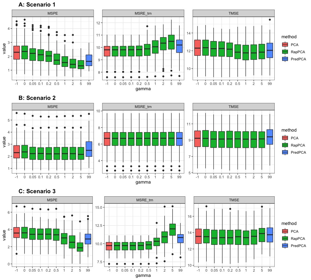
Figure 1: Breakdown of MSPE, MSRE-trn (which is MSRE on the training set) and TMSE for the first PC by $\gamma$ arcoss 100 replicates of data, with classical PCA (coded as $\gamma=-1$) and predictive PCA (PredPCA, coded as $\gamma=99$) results presented for reference

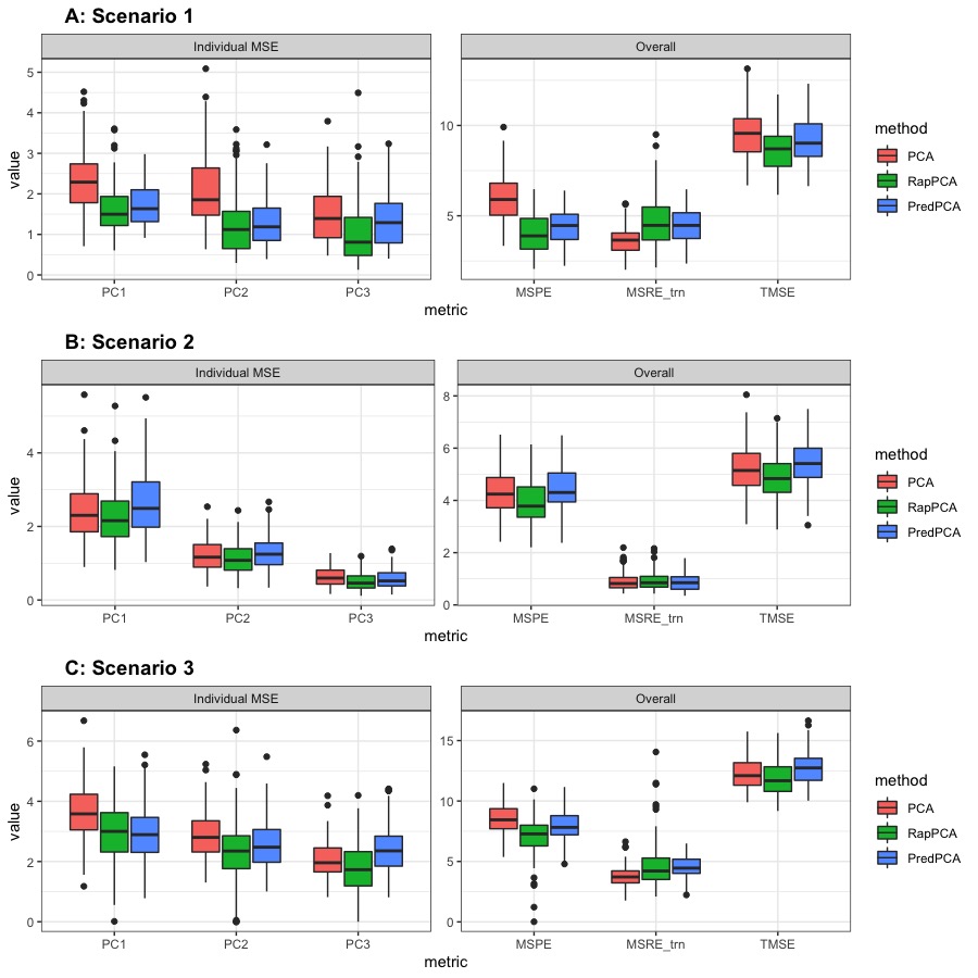
Figure 2: Individual prediction MSEs for each PC (left) and overall metrics for all PCs (right) across 100 replicates of data. The optimal tuning parameters $\gamma,\lambda_{1}$ and $\lambda_{2}$ are selected separately for each simulation by minimizing TMSE via cross-validation.

4.2 Scenario 2: PCs with Unequal Contribution

We now consider a scenario where the predictable PCs explain a higher proportion of variability than the unpredictable PCs. In particular, the simulation setting is similar to Scenario 1, except that the entries of $\tilde{M}$ are first drawn from independent Uniform$[-1,1]$ distributions, and then the rows are scaled to have decaying norm (recall that the first 3 PCs are more predictable than the last 3 PCs). In contrast to Scenario 1, we expect in this case that PCA and predictive PCA would have comparable prediction, approximation and overall accuracy, since the well-predictable components of $Y$ coincide with those that explain the greatest amount of variance.

For the same reason, adjusting $\gamma$ in this case would not lead to steep changes in MSPE, MSRE or TMSE for RapPCA, as reflected by the flat curves of each metric in Panel B of Figure 1. Despite the similar behaviors of PCA and predictive PCA, Panel B of Figure 2 reveals that RapPCA is still able to improve the prediction and overall performance by more flexibly exploiting the covariate and spatial information when identifying the PCs.

4.3 Scenario 3: PCs with Non-Linear Mean

In our last simulation, we investigate the setting where the relationship between the true PCs and the covariates is non-linear. We modify the setting in Scenario 1 so that

$$f_{l}(X)=X^{\odot 2}\beta_{l}+2\sum_{j=1}^{\lfloor d/2\rfloor}(X_{2j-1}\odot X_{2j})\alpha_{lj},$$

for $l=1,2,3$, where $\odot$ and $\odot^{2}$ denote element-wise multiplication and square, and $\lfloor x\rfloor$ denotes the largest integer not exceeding $x$. In other words, we specify the mean function to be a combination of squared and interaction terms of the covariates, where interactions exist between pairs of consecutive covariates ($X_{\cdot 1}$ and $X_{\cdot 2}$; $X_{\cdot 3}$ and $X_{\cdot 4}$, etc).

Panel C of Figure 1 indicates that the flexibility of handling non-linear effects enables a clear advantage in prediction accuracy for RapPCA compared with both predictive and classical PCA in this scenario, when we impose a large enough penalty $\gamma$ on prediction errors in optimization. It is not surprising that putting an emphasis on prediction leads to some loss in approximation accuracy; however, we could observe from Panel C of Figure 2 that by controlling such balance in a data-adaptive way, RapPCA is able to achieve meaningful improvement in MSPE while maintaining comparable, if not superior, overall performance.

4.4 Remarks on the Predictability-Representability Trade-Off

In all of our simulation studies, we choose the key tuning parameter $\gamma$ of RapPCA data-adaptively by minimizing TMSE in cross-validation. While TMSE is a comprehensive and balanced metric to use for tuning, alternative choices can be made with considerations on the practical use cases.

For example, in health effect studies of air pollution with spatial misalignment between the locations of measured health outcomes and those of measured pollutant concentrations, the accuracy of such spatial extrapolation is arguably more important than the closeness of approximation for the original pollution measurements (Jandarov et al., 2017). In this case, researchers may examine the breakdown of metrics in cross-validation similar to Figure 1 and manually select a value of $\gamma$ leading to satisfying prediction accuracy (MSPE) without significantly compromising MSRE or TMSE. We also note from the curvature of TMSE versus $\gamma$ in these figures that for many practical cases, the overall performance of RapPCA is not too sensitive to the choice of $\gamma$, or the metric(s) used to select it. In other words, manually adjusting the predictability-representability trade-off with RapPCA leads to consistently improved predictability and better, or at least similar, overall accuracy (TMSE) compared with existing methods such as PCA and predictive PCA.

5 Applications

We illustrate the utility of RapPCA using real datasets in two different domain areas — environmental epidemiology and spatial transcriptomics. The first application of dimension reduction in Section 5.1 ($n=309,\ p=23$) represents the case where practitioners seek to improve predictability (MSPE) and the overall performance (TMSE), and hence RapPCA is able to explicitly optimize these metrics as desired. The second example in Section 5.2 ($n=607,\ p=10,053$) includes the scenario where tasks other than spatial prediction (e.g., clustering) are of interest; we demonstrate that RapPCA, though not directly incorporating the ultimate goal into optimization, is able to capture meaningful biological and spatial information in the extracted PCs by enforcing predictability, leading to desirable model performance.

5.1 Analysis of Seattle Traffic-Related Air Pollution Data

The performance of RapPCA in comparison with common existing methods, including classical and predictive PCA, is first illustrated with the multivariate traffic-related air pollution (TRAP) data in Seattle (Blanco et al., 2022). The study leverages a mobile monitoring campaign where a vehicle equipped with air monitors repeatedly collected two-minute samples at $n=309$ stationary roadside sites in the greater Seattle area. Repeated samples for the concentrations of 6 types of pollutants were obtained, including ultrafine particles (UFP), black carbon (BC), nitrogen dioxide (NO₂), carbon monoxide (CO), carbon dioxide (CO₂) and fine particulate matter (PM_2.5). Due to data quality considerations, we focus on UFP, BC and NO₂ in our analysis. For UFP and BC, the concentrations were measured with multiple instruments corresponding to different measurement ranges or units. In particular, NanoScan instrument with 13 different bin sizes, as well as DiSCmini and PTRAK 8525 (with and without diffusion screen) instruments measured the concentration of UFP in terms of the counts of particles with different size ranges, along with the median size and overall count of particles. Black carbon was assessed by micro-aethalometer (MA200), which measures the concentration of particles with different light absorbing properties, corresponding to 5 different ranges of wavelengths.

The median 2-minute visit concentrations were winsorized at the site level such that concentrations below the 5^th and above the 95^th quantile for a given site site were set to those thresholds, respectively. This was done to reduce the influence of outliers in the measurements. These winsorized medians were then averaged for each site, leading to $p=23$ annual average measurements of pollutant concentrations in total, including 17 for UFP, 5 for BC, and one for NO₂. We use the concentration of NO₂ to normalize all other variables except the median size measurements for UFP from the DiSCmini. All variables are centered and scaled before running each PCA algorithm.

We are interested in extrapolating the pollutant measurements to unobserved locations in the same study region. Because of the autocorrelation between these measurements, predicting each of them separately might not always lead to sensible results; instead, dimension reduction is needed before building spatial prediction models. Dimension reduction also allows us to understand the health effects of pollutant mixtures rather than separate pollutants alone. As in Section 4, we compare the performance of RapPCA with classical and predictive PCA, each extracting the top 3 PCs from the 23 measurements of air pollutants. Due to the high dimensionality of geographical covariates, we first ran PCA on these 189 covariates and used the top 15 PCs as predictors for predictive PCA. PCA and RapPCA were applied without this additional step. We examine the overall metrics as well as the individual prediction MSEs for each PC via 10-fold cross-validation, where the same spatial prediction approach as Section 4 is followed, namely, a random forest model followed by spatial smoothing via TPRS on the residuals (Wai et al., 2020).

Table 1 compares each dimension reduction algorithm in terms of cross-validated TMSE, MSPE and MSRE-trn as well as prediction MSEs for each PC. Consistent with the findings from simulation studies, RapPCA achieves the lowest prediction and overall errors, while PCA has the smallest approximation gap on the training data. The advantage in predictability of RapPCA is reflected in both the overall MSPE and the individual MSEs for each PC. In this particular data analysis task, predictive PCA has good predictive performance for the second PC but is otherwise similar to or outperformed by both classical PCA and RapPCA. More generally, in settings with high-dimensional predictors (covariates and/or spatial basis), predictive PCA is not guaranteed to show an advantage in predictability since it requires a separate processing step on these predictors instead of selecting the information to use for prediction data-adaptively as RapPCA does.

	Overall Metrics			Individual MSEs
	TMSE	MSPE	MSRE-trn	PC1	PC2	PC3
PCA	14.79	7.93	6.38	3.93	2.86	1.14
PredPCA	14.81	7.16	7.28	3.41	2.53	1.22
RapPCA	13.92	6.66	6.75	2.62	2.92	1.12

Table 1: Comparison of overall metrics and individual prediction MSEs for each PC, assessed by 10-fold cross-validation on the Seattle traffic-related air pollution data

We then run dimension reduction with each of the PCA algorithms on the whole dataset to assess the spatial distribution of top 3 PC scores, where for RapPCA we select the tuning parameters $\gamma,\lambda_{1}$ and $\lambda_{2}$ that lead to the optimal TMSE. Next, we train spatial prediction models for each of the PC scores, and evaluate these models on a finer grid of 5,040 locations over the study region to obtain smoothed plots of each PC score. Figure 3 visualizes the smoothed PC scores obtained by each method across the study region, and Figure 4 presents the PC loadings reflecting the contribution of each pollutant on the PC scores. We observe similar spatial patterns in the distribution of the PC scores across different methods, except for the south end of the study region for the third PC where PCA identifies a stronger signal than RapPCA and predictive PCA. In particular, all methods highlight regions near the airport and/or around major roads (the dark red area) for the first PC, indicating aircraft and road traffic emissions as a major source of overall pollution level. This is consistent with the large contributions of BC as well as UFP with small or moderate sizes (Zhang et al., 2019; Bendtsen et al., 2021), as reflected by the loadings of UFP (with relatively small particle sizes) and BC in Figure 4.

Roughly categorizing various UFP particle sizes into small, moderate and large groups, one key difference we observe from Figure 4 between RapPCA and the two benchmark algorithms is that RapPCA identifies one size group to be the main contributor to each of the 3 PCs, while the other two groups have negligible loadings: small particles contributing to the top PC, moderately-sized particles to the second PC, and large ones to the third PC. In addition, BC is mainly contributing to the second PC according to RapPCA. This observation is consistent with findings from other studies, where aircraft emissions (primarily composed of small UFPs) and road traffic, especially diesel exhaust (comprising moderately-sized UFPs and BC), were identified as two key sources of traffic-related air pollution (Austin et al., 2021; Nie et al., 2022). In contrast, neither predictive nor classical PCA effectively distinguishes the contributions of UFPs with different sizes or the contribution of BC.

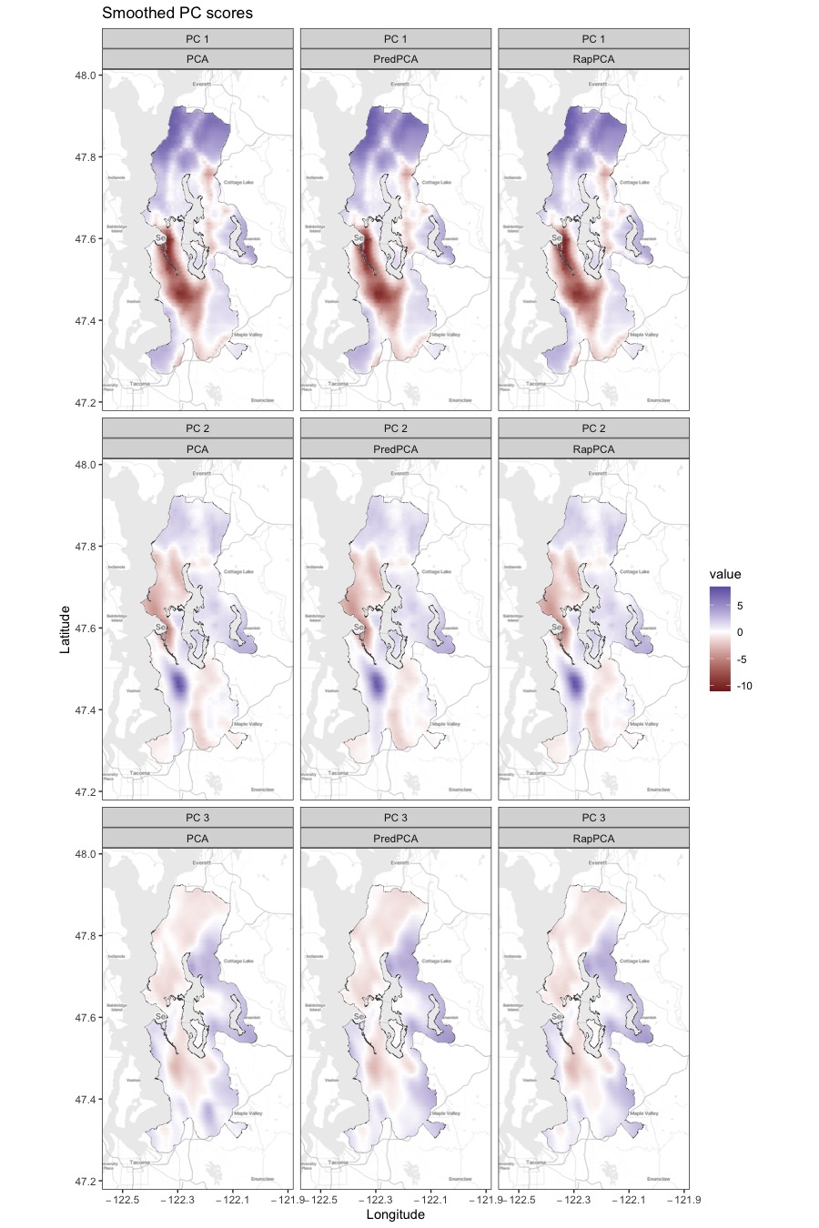
Figure 3: Smoothed PC scores of pollutant concentrations from the Seattle TRAP data

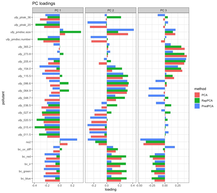
Figure 4: PC loadings for each pollutant. There are 3 types of pollutants, where the suffix, if applicable, represents the properties of, or the instruments used to measure, each pollutant. In particular, the numeric suffix after ufp_ corresponds to the range of sizes for the particles. ufp_ptrak_36 represents PTRAK measurements with diffusion screen, and ufp_ptrak_20 represents the difference between PTRAK measurements without and with diffusion screen. Black carbon (BC) measurements at different wavelengths are shown: blue (bc_blue), green (bc_green), infrared (bc_ir), red (bc_red), and ultraviolet (bc_uv). Ultraviolet measurements were transformed to represent the difference (bc_uv_diff) between ultraviolet and infrared ranges.

5.2 Analysis of HER2-Positive Breast Tumor Spatial Transcriptomics

In this section, we present another use case of RapPCA by analyzing spatial transcriptomics data. While dimension reduction is also a common data handling step in these applications, there are a variety of downstream modeling tasks where spatial prediction, as in the Seattle TRAP study, may not be the primary focus. We will nevertheless illustrate that optimizing the balance between predictability and representability with RapPCA still leads to desirable performance in these tasks.

We analyze the human epidermal growth factor receptor 2 positive (HER2+) breast tumor data, which includes expression measures of genes in HER2+ tumors from eight individuals (Andersson et al., 2021). We focus on the first tumor section of the last individual, coded as sample H1 in Andersson et al. (2021), where the data consists of expression counts of $15,030$ genes on $613$ tissue locations. Following the same filtering steps as in Shang and Zhou (2022), we removed genes with non-zero expression at less than 20 locations and those confounded by technical artifacts (Andersson et al., 2021), as well as locations with non-zero expressions for less than 20 genes. The filtered set of data contains $10,053$ genes measured on $607$ spots, which is then normalized via regularized negative binomial regression as implemented by the Seurat R package (Hafemeister and Satija, 2019).

Due to the large number of genes along with the noise present in the expression measurements (Rao et al., 2021), dimension reduction is commonly done before the main analytic tasks on genomic data to extract biologically meaningful signals as well as to facilitate computation; see Sun et al. (2019); Zhao et al. (2021); Shang and Zhou (2022) for related examples. We focus on two modeling tasks: spatial extrapolation and domain detection. In addition to the three PCA methods (PCA, predictive PCA, RapPCA) that were investigated in previous sections, we also include spatial PCA for comparison, which is a probabilistic PCA algorithm for spatial transcriptomics data incorporating spatial proximity information in the modeling of PC scores (Shang and Zhou, 2022).

The first application is more similar to the analysis in Section 5.1, where we are interested in predicting the gene expression PC scores at tissue locations with no measurements. This prediction problem is involved, for example, in the reconstruction of high-resolution spatial maps of gene expression (Gryglewski et al., 2018; Shang and Zhou, 2022). For each dimension reduction method, we extract the top 20 PCs from the expression of all genes, and conduct 10-fold cross-validation to assess TMSE, MSPE and MSRE-trn, where spatial prediction is done by random forest followed by TPRS smoothing as in previous sections. For spatial PCA, we also include results from its built-in spatial prediction function (from the SpatialPCA R package) for completeness. Table 2 summarizes the overall metrics along with individual prediction MSEs for the top 3 PCs. RapPCA demonstrates significant advantage in overall prediction accuracy (MSPE) compared to all other methods, followed by predictive PCA which also has the lowest per-PC MSEs for the top 3 PCs. Also, consistent with findings from previous sections, RapPCA achieves the optimal trade-off between prediction and approximation gaps, as reflected by TMSE.

	Overall Metrics			Individual MSEs
	TMSE	MSPE	MSRE-trn	PC1	PC2	PC3
PCA	272.21	32.24	239.97	6.64	5.09	3.18
PredPCA	278.08	31.85	246.15	3.93	4.12	2.26
SpatialPCA	292.78	46.09	246.70	6.84	5.89	3.69
SpatialPCA: built-in	296.59	49.90	246.70	6.81	5.96	3.81
RapPCA	271.35	20.56	250.80	5.59	4.86	3.79

Table 2: Comparison of overall metrics and individual prediction MSEs for each of the top 3 PCs, assessed by 10-fold cross-validation on the breast tumor data

Figure 5 shows the top 3 PC scores from the expressions of all genes. We observe that spatial PCA and predictive PCA produce spatially smoother surfaces of PC scores compared to the other two methods. This is natural for predictive PCA since it prioritizes spatial predictability of the PC scores which results in stronger spatial smoothing; while for spatial PCA, the prediction-representation balance is implicit and less straightforward to interpret. The gap in prediction performance comparing spatial or predictive PCA with RapPCA may be the consequence of over-smoothing, which also indicates the effectiveness of explicit optimization for the prediction-representation balance achieved by (3). Figure 11 in Appendix B.2 visualizes the smoothed high-resolution maps of PC scores based on predictions at unmeasured locations.

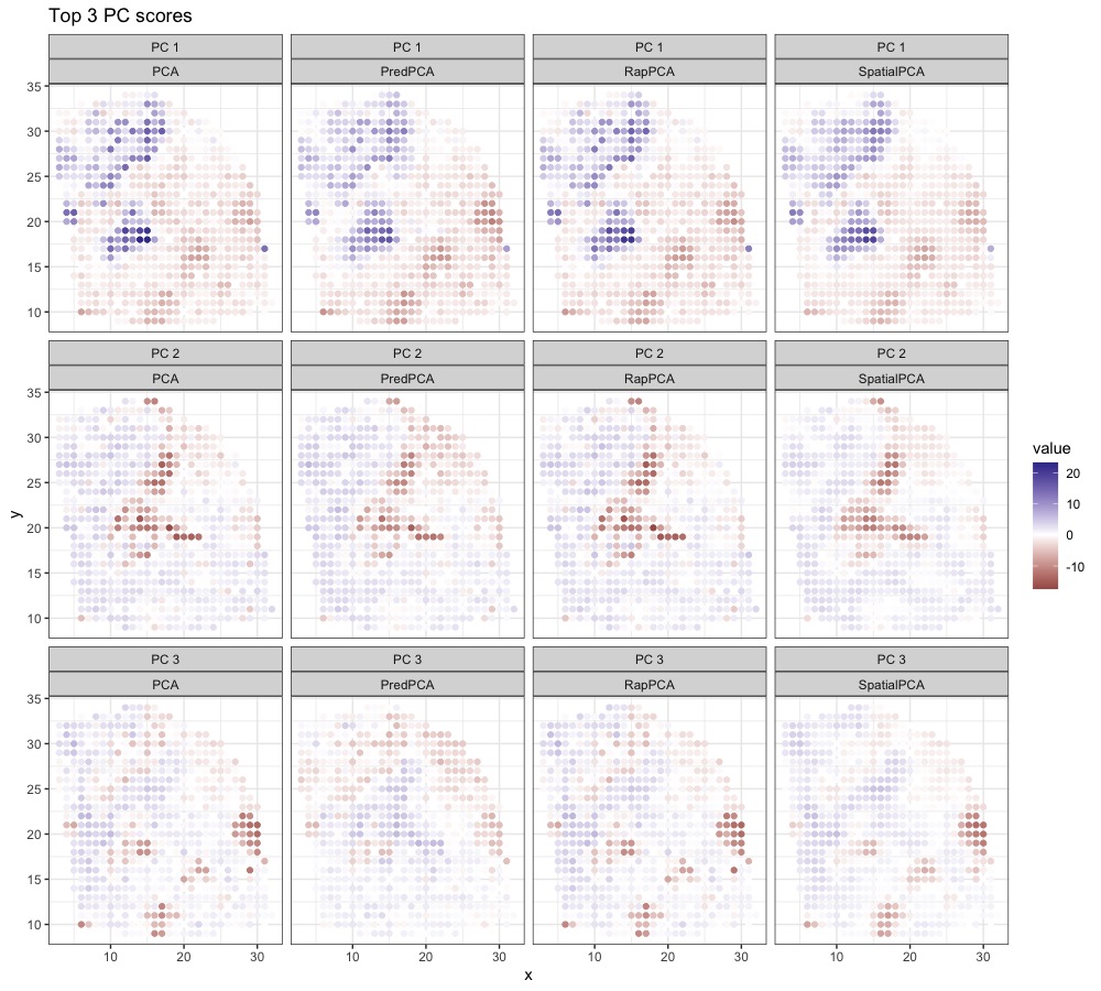
Figure 5: Top 3 PC scores based on gene expression in the HER2-positive breast tumor data

As a second example, we investigate the problem of domain detection following the dimension reduction step. Domain detection is the task where different sections of tissues are identified as various spatially coherent and functionally distinct regions (Dong and Zhang, 2022; Shang and Zhou, 2022), providing helpful insights into the biological function of tissues. To this end, we conduct domain detection via walktrap clustering algorithm (Pons and Latapy, 2005) using the top 20 PCs extracted by each variant of PCA. The number of clusters is set to align with the “ground truth” labels based on pathologist annotations of tissue regions in the original study (Andersson et al., 2021). The hyperparameters $\gamma,\lambda_{1},\lambda_{2}$ are chosen based on silhouette value measuring the difference between nearest-cluster versus intra-cluster distances.

Figure 6 visualizes the detected spatial domains based on PCs extracted from different dimension reduction procedures, compared to the ground truth labels. In general, the relative performance of each approach differs across spatial domains. For example, PCA fails to detect the adipose tissue region and produces noisier results for regions surrounding invasive cancer cells. Predictive PCA and RapPCA both mis-classify part of the cancer in situ region as invasive cancer, where predictive PCA results are noisier for the top left region, and RapPCA shows larger uncertainty regarding adipose tissue. Spatial PCA, on the other hand, infers part of the connective tissue to be cancerous.

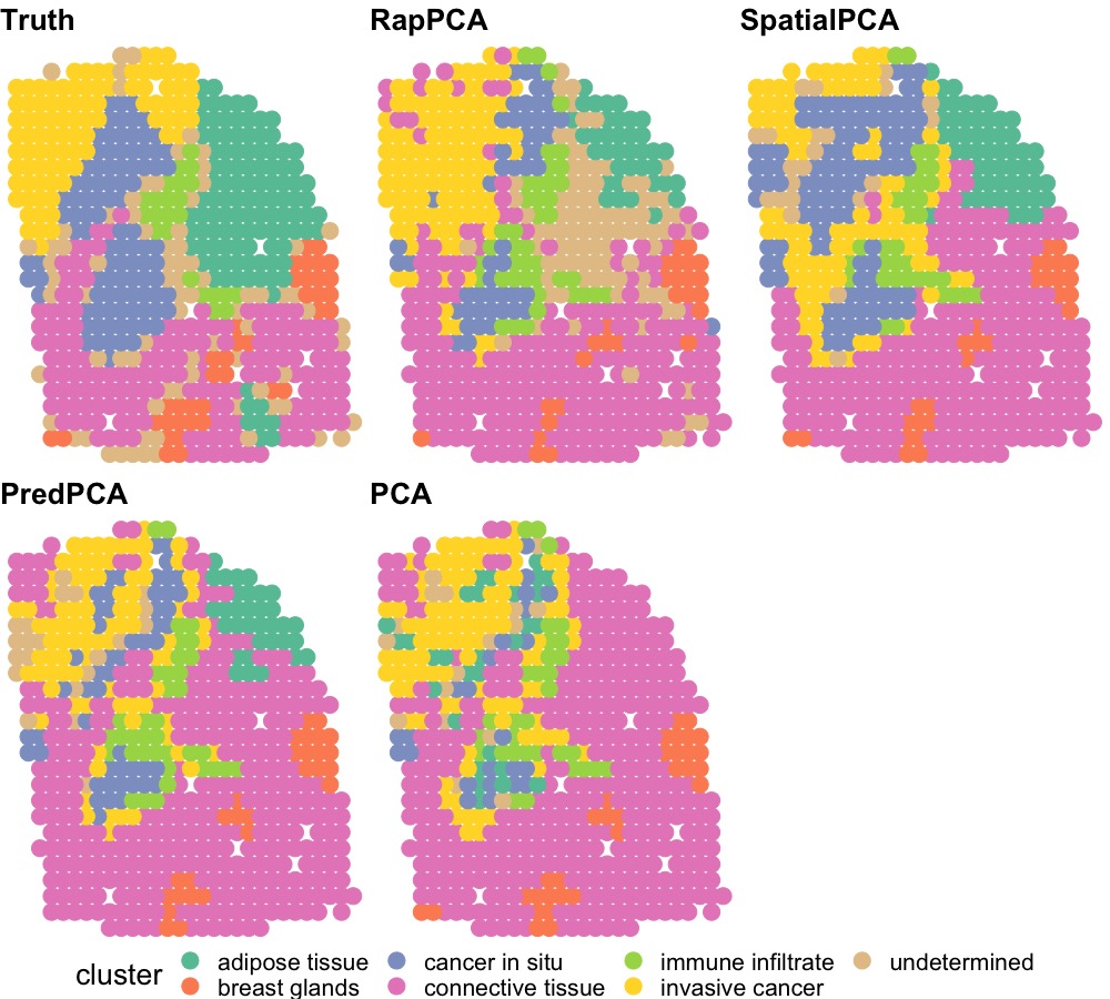
Figure 6: Detected spatial domains and annotated ground truth

To make a more in-depth comparison, we examine the breakdown of clustering accuracy by ground truth labels, in other words, whether or not each approach correctly classifies the spots belonging to each spatial domain, with the undetermined cluster removed from comparison. Figure 7 presents this breakdown for each method in terms of precision, recall and F1 score as a composite measure. As observed from the spatial domain plots, the relative accuracy for each method differs by region, and in particular, RapPCA has the best performance in both precision and recall on the identification of invasive cancer regions, whereas spatial PCA shows an advantage in recall for cancer in situ.

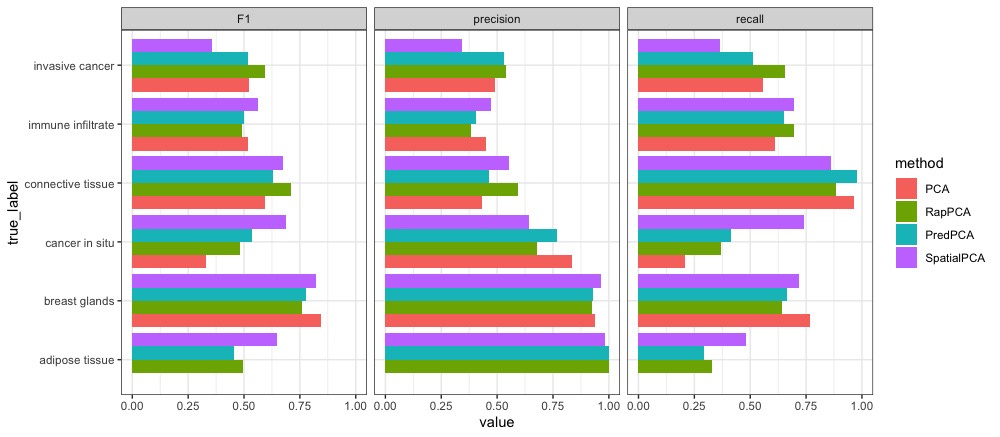
Figure 7: Breakdown of domain detection accuracy by true label. Note that the metrics for the adipose tissue region are not well-defined for PCA because it fails to detect any spot in this region.

6 Discussion

When dimension reduction is conducted as an intermediate step before a spatial modeling task of interest, there are two typically conflicting considerations guiding the choice of approaches. The more obvious one is how closely the lower dimensional score represents the original variables, which we refer to as representability. Another important aspect is the predictability of the resulting scores, i.e., how well they could be expressed or predicted by available covariates and/or spatial effects.

We discussed how existing dimension reduction algorithms fit into this general framework of optimizing either criterion, and proposed a flexible interpolation between them that achieves the optimal representability-predictability trade-off. Our proposal, called RapPCA, can also handle high-dimensional covariates and non-linear relationships. Simulation studies under different scenarios illustrate the gain in downstream prediction accuracy by our method, which also achieves smaller overall errors when both predictability and representability are taken into account. Applications to real datasets in different scientific areas further demonstrate the utility of our proposed method, even in analytic tasks that do not explicitly involve prediction.

The balance between prediction and representation performance can be viewed as a generalized form of bias-variance trade-off. While methods such as classical PCA minimize the representation gap specifically for the training data at hand, such representation may capture excessive noise if it explains a large amount of variability in the data. In contrast, the formulation of predictive PCA restricts the PC scores to fall within a certain model space, the linear span of the covariates, which is a form of regularization enforcing the smoothness of the PCs. Many probabilistic dimension reduction approaches implicitly address both aspects, while our proposal seeks the optimal balance in an explicit and interpretable way.

While we used TMSE to guide the choice of tuning parameters in our examples, in practice tuning parameter selection could be driven by the specific analytic goal in practice. Researchers could examine the trend of prediction, representation and total errors by each tuning parameter, and in particular $\gamma$ in (3), on a set of test data, and choose the combination leading to a desired trade-off. Our empirical evaluations suggest that striking such balance with our proposed method would most often improve, or at least maintain similar, overall errors compared to existing alternatives.

The procedure described in Algorithm 1 depends on a specified number $r$ of PCs. Since increasing $r$ will reduce the total MSRE and increase the total MSPE, one could examine the trajectory of MSPE and MSRE with respect to $r$, and identify the elbow of these curves as a practical choice of $r$; this reflects the threshold beyond which adding more PCs would not alter either the prediction or representation meaningfully. Practitioners may also be interested in estimating the variability of evaluation metrics such as TMSE, MSPE and MSRE to better understand the trade-off between them. While our method does not directly provide uncertainty estimates, one could conduct bootstrap to assess this, with the potential caveat of sample splitting on correlated samples. Though Theorem 1 establishes an exact solution to the optimization problem (3) that, in theory, does not contain numerical errors, computational inaccuracy may occur in scenarios with large sample size or high dimensionality, since the quality of eigen-decomposition could suffer when the condition number of the matrix involved is large. Alternative numerical techniques could improve the accuracy and stability of the proposed dimension reduction procedure.

APPENDIX

Appendix A Proof

Proof of Theorem 1.

For the $l$th component, denote the singular value decomposition of $Y^{(l)}$ as $Y^{(l)}=\mathcal{S}^{(l)}{\mathcal{D}^{(l)}}{\mathcal{T}^{(l)}}^{\top}$. Let ${\eta}:=\left[\alpha^{\top}\quad\sqrt{\frac{\lambda_{2}}{\lambda_{1}}}\beta^{\top}\right]^{\top}$, $Z:=\left[K\quad\sqrt{\frac{\lambda_{2}}{\lambda_{1}}}B\right]$, and let the combined penalty matrix be

$$P:=\begin{bmatrix}\tilde{K}&0\\ 0&\frac{\lambda_{2}}{\lambda_{1}}\tilde{Q}\end{bmatrix}.$$

We verify that the optimization problem (3) has a unique global minimizer given by

• $\tilde{v}$ as defined in Algorithm 1;

• $\tilde{\eta}=(\gamma Z^{\top}Z+\lambda_{1}P)^{-1}(\gamma Z^{\top}\mathcal{S}^{(l)}{\mathcal{D}^{(l)}}q)$, with $q$ defined as in Algorithm 1;

by doing so, we establish the optimality of our solution given by Algorithm 1.

Recall the form of the optimization problem given in (3):

$$\min_{v,\alpha,\beta}\ f_{\gamma,\lambda_{1},\lambda_{2}}(v,\alpha,\beta):=\left\lVert Y^{(l)}-Y^{(l)}vv^{\top}\right\rVert_{F}^{2}+\gamma\left\lVert Y^{(l)}v-(K\alpha+B\beta)\right\rVert_{2}^{2}+\lambda_{1}\alpha^{\top}\tilde{K}\alpha+\lambda_{2}\beta^{\top}\tilde{Q}\beta$$

$$\text{s.t. }v^{\top}v=1.$$

The superscript $(l)$ will be suppressed for simplicity. We denote $y=Y^{(l)}$ and start by examining the first term in the objective function, which, under the constraint, can be expressed as

$$\left\lVert Y^{(l)}-uv^{\top}\right\rVert_{F}^{2} =\text{tr}\left((y-uv^{\top})^{\top}(y-uv^{\top})\right)$$

$$=\text{tr}\left(y^{\top}y-2y^{\top}yvv^{\top}+vv^{\top}y^{\top}yvv^{\top}\right)$$

$$\propto-2\text{tr}\left(v^{\top}{\mathcal{T}}\mathcal{D}\mathcal{S}^{\top}\mathcal{S}\mathcal{D}{\mathcal{T}}^{\top}v\right)+\text{tr}\left(v^{\top}vv^{\top}{\mathcal{T}}\mathcal{D}{\mathcal{S}}^{\top}{\mathcal{S}}\mathcal{D}{\mathcal{T}}^{\top}v\right),$$ (4)

where $\text{tr}(\cdot)$ denotes the trace of a matrix, $\propto$ means equal up to a constant not depending on $u,v,\alpha$ or $\beta$, and we have made use of the cyclic property of trace. Since $v^{\top}v=1$ and ${\mathcal{S}}^{\top}{\mathcal{S}}=I$, denoting $q:={\mathcal{T}}^{\top}v$, (4) continues as

$$\left\lVert Y^{(l)}-uv^{\top}\right\rVert_{F}^{2} =-2\text{tr}\left(q^{\top}\mathcal{D}^{2}q\right)+\text{tr}\left(q^{\top}\mathcal{D}^{2}q\right)=-{q^{\top}\mathcal{D}^{2}q}.$$

Under the reparametrization in Theorem 1, namely, ${\eta}:=\left[\alpha^{\top}\quad\sqrt{\frac{\lambda_{2}}{\lambda_{1}}}\beta^{\top}\right]^{\top}$ and $Z:=\left[K\quad\sqrt{\frac{\lambda_{2}}{\lambda_{1}}}B\right]$, the objective function becomes

$$f_{\gamma,\lambda_{1},\lambda_{2}}(v,\eta) =-q^{\top}\mathcal{D}^{2}q+\gamma\left\lVert{\mathcal{S}}\mathcal{D}q-Z\eta\right\rVert_{2}^{2}+\lambda_{1}\eta^{\top}P\eta,$$

which is a quadratic function of $\eta$ for fixed $q$, with

$$\frac{\partial f}{\partial\eta}=2\gamma Z^{\top}(Z\eta-{\mathcal{S}}\mathcal{D}q)+2\lambda_{1}P\eta.$$

Since the Hessian $\partial^{2}f/\partial\eta^{2}=2\gamma Z^{\top}Z$ is positive semidefinite, we can profile out $\eta$ by setting it to the minimizer $\tilde{\eta}(q):=(\gamma Z^{\top}Z+\lambda_{1}P)^{-1}(\gamma Z^{\top}{\mathcal{S}}\mathcal{D}q)$. The objective function can thus be rearranged as

$$f_{\gamma,\lambda_{1},\lambda_{2}}(v,\alpha,\beta) :=g_{\gamma,\lambda_{1}}(q,\tilde{\eta})=-q^{\top}\mathcal{D}^{2}q+\gamma({\mathcal{S}}\mathcal{D}q-Z\tilde{\eta})^{\top}({\mathcal{S}}\mathcal{D}q-Z\tilde{\eta})+\lambda_{1}\tilde{\eta}^{\top}P\tilde{\eta}$$

$$=-q^{\top}\mathcal{D}^{2}q+\gamma(q^{\top}\mathcal{D}^{2}q-2\tilde{\eta}^{\top}Z^{\top}{\mathcal{S}}\mathcal{D}q+\tilde{\eta}^{\top}Z^{\top}Z\tilde{\eta})+\lambda_{1}\tilde{\eta}^{\top}P\tilde{\eta}$$

$$=(\gamma-1)q^{\top}\mathcal{D}^{2}q-2\gamma^{2}q^{\top}\mathcal{D}{\mathcal{S}}^{\top}Z(\gamma Z^{\top}Z+\lambda_{1}P)^{-1}Z^{\top}{\mathcal{S}}\mathcal{D}q$$

$$\quad\quad+\gamma^{2}q^{\top}\mathcal{D}{\mathcal{S}}^{\top}Z(\gamma Z^{\top}Z+\lambda_{1}P)^{-1}(\gamma Z^{\top}Z+\lambda_{1}P)(\gamma Z^{\top}Z+\lambda_{1}P)^{-1}Z^{\top}{\mathcal{S}}\mathcal{D}q$$

$$=-q^{\top}\left[-(\gamma-1)\mathcal{D}^{2}+\gamma^{2}\mathcal{D}{\mathcal{S}}^{\top}Z(\gamma Z^{\top}Z+\lambda_{1}P)^{-1}Z^{\top}{\mathcal{S}}\mathcal{D}\right]q:=-q^{\top}Aq,$$ (5)

where $A:=-(\gamma-1)\mathcal{D}^{2}+\gamma^{2}\mathcal{D}{\mathcal{S}}^{\top}Z(\gamma Z^{\top}Z+\lambda_{1}P)^{-1}Z^{\top}{\mathcal{S}}\mathcal{D}$.

It then follows that the original optimization problem (3) is equivalent to

$$\min_{q}\ f_{\gamma,\lambda_{1}}(q):=-q^{\top}Aq\quad\text{s.t. }q^{\top}q=1,$$

for which the optimal solution is the normalized first eigenvector of $A$ (i.e., the one corresponding to the largest eigenvalue). By construction and the properties of eigendecomposition, such $q$ is guaranteed to be the global minimizer of $f_{\gamma,\lambda_{1}}(q)$. Recalling the form of $\tilde{\eta}(q)$ and the fact that the untransformed optimal solution satisfies ${\mathcal{T}}^{\top}\tilde{v}=\tilde{q}$ and $\tilde{u}=Y^{(l)}\tilde{v}$ completes the proof. ∎

Appendix B Additional Numerical Results

B.1 Optimality of Proposed Solution

We use the first replicate (out of 100 total) of data in Simulation Scenario 1 (Section 4.1) to numerically verify our claim in Theorem 1, i.e., the optimality of the derived solution.

Specifically, we solve the optimization problem (3) to extract the first PC score, and vary the first two entries of the optimal loadings $\tilde{v}$ while keeping everything else (including the PC scores $\tilde{u}$ and coefficients $\tilde{\eta}$) intact, and ensuring that the constraint $v^{\top}v$ is still satisfied. This is done under polar coordinates: letting $\theta\in[0,2\pi)$, we write $v^{*}(\theta)$ as the modified loading vector, where the entries $v_{j}^{*}(\theta)=\tilde{v}_{j}$ for $j>2$. We let $v^{*}_{1}(\theta)=\rho\sin\theta$ and $v^{*}_{2}(\theta)=\rho\cos\theta$ where $\rho=\sqrt{1-\sum_{j>2}{\tilde{v}_{j}}^{2}}$. Then, as $\theta$ varies within $[0,2\pi)$, the two entries $(v_{1}^{*}(\theta),v_{2}^{*}(\theta))$ take all possible combinations that satisfy the constraint.

We explore different values of tuning parameters $\gamma,\lambda_{1},\lambda_{2}$ and compare the objective function $f_{\gamma,\lambda_{1},\lambda_{2}}(u,v,\eta)$ evaluated at the optimal solution $(\tilde{u},\tilde{v},\tilde{\eta})$ versus the modified solution $(\tilde{u},v^{*}(\theta),\tilde{\eta})$ for $\theta\in[0,2\pi)$. We plot their differences against $\theta$ for various values of tuning parameters in Figures 8 and 9. Note that the optimal $\theta$, i.e., the value leading to the optimal loading $v^{*}(\theta)$, may differ with different sets of tuning parameters $\gamma,\lambda_{1}$ and $\lambda_{2}$. The fact that each curve is always above or equal to zero, and reaches zero exactly once, verifies the uniqueness of the optimal solution, as well as the optimality of the proposed form of $\tilde{v}$, at least for fixed $\tilde{u}$ and $\tilde{\eta}$.

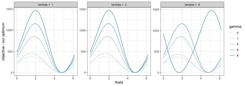
Figure 8: Difference between the objective function evaluated over a range of values for the first two parameters in the loading vector and the optimum achieved by our algorithm. The $x$-axis is parameterized by $\theta$, the polar coordinate angular representation of the candidate parameters, and we fix $\lambda_{1}=\lambda_{2}$. Each panel corresponds to a value of $\lambda_{1}$ and $\lambda_{2}$.

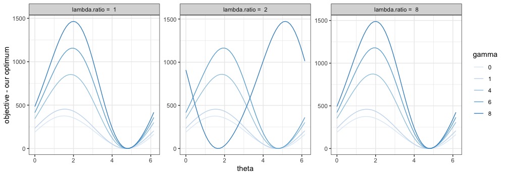
Figure 9: Difference between the objective function evaluated over a range of values for the first two parameters in the loading vector and the optimum achieved by our algorithm. The $x$-axis is parameterized by $\theta$, the polar coordinate angular representation of the candidate parameters, and we fix $\lambda_{1}=1$. Each panel corresponds to a value of the ratio $\lambda_{2}/\lambda_{1}$.

B.2 Additional Simulation and Data Analysis Results

Figure 10 is an analog to Figure 1 presented in our simulation studies, which visualizes the variation of TMSE, MSPE and MSRE-trn for the first PC with respect to the combination of $\lambda_{1}$ and $\lambda_{2}$. For each combination, the additional tuning parameter $\gamma$ is chosen such that it leads to the lowest TMSE. In Scenarios 1 through 3, the median values of the selected parameters $(\lambda_{1},\lambda_{2}/\lambda_{1})$ via cross-validation are (0.5, 1), (1, 0.75) and (0.5, 0.25) respectively, all of which are reasonably close to near-optimal region(s) in Figure 10.

Figure 10: Average TMSE, MSPE and MSRE-trn for the first PC arcoss 100 replicates of data, plotted against the combination of $\lambda_{1}$ and the ratio $\lambda_{2}/\lambda_{1}$.

Figure 11 presents the smoothed high-resolution maps of predicted PC scores, obtained by each dimension reduction approach. We observe that predictive PCA produces the smoothest predicted map due to its emphasis on the predictability of PC scores; however, it could over-smooth and omit meaningful spatial variations in gene expression, as can be seen in the high-resolution map for the third PC. For spatial PCA, while the extracted low-resolution PCs also demonstrate smoothness as predictive PCA (see Figure 5), they are not guaranteed to be well predictable and the extrapolated high-resolution map appears noisier. RapPCA achieves a reasonable balance among all algorithms.

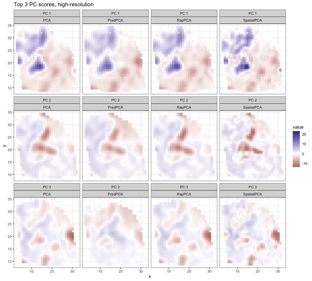
Figure 11: Smoothed PC scores based on predicted high-resolution gene expression maps in the HER2-positive breast tumor data

References

- Achilleos et al. (2017) Achilleos, S., Kioumourtzoglou, M.-A., Wu, C.-D., Schwartz, J. D., Koutrakis, P. and Papatheodorou, S. I. (2017) Acute effects of fine particulate matter constituents on mortality: A systematic review and meta-regression analysis. Environment International, 109, 89–100.
- Andersson et al. (2021) Andersson, A., Larsson, L., Stenbeck, L., Salmén, F., Ehinger, A., Wu, S. Z., Al-Eryani, G., Roden, D., Swarbrick, A., Borg, Å. et al. (2021) Spatial deconvolution of HER2-positive breast cancer delineates tumor-associated cell type interactions. Nature Communications, 12, 6012.
- Austin et al. (2021) Austin, E., Xiang, J., Gould, T. R., Shirai, J. H., Yun, S., Yost, M. G., Larson, T. V. and Seto, E. (2021) Distinct ultrafine particle profiles associated with aircraft and roadway traffic. Environmental Science & Technology, 55, 2847–2858.
- Bendtsen et al. (2021) Bendtsen, K. M., Bengtsen, E., Saber, A. T. and Vogel, U. (2021) A review of health effects associated with exposure to jet engine emissions in and around airports. Environmental Health, 20, 1–21.
- Bergen et al. (2013) Bergen, S., Sheppard, L., Sampson, P. D., Kim, S.-Y., Richards, M., Vedal, S., Kaufman, J. D. and Szpiro, A. A. (2013) A national prediction model for PM2.5 component exposures and measurement error-corrected health effect inference. Environmental Health Perspectives, 121, 1017–1025.
- Blanco et al. (2022) Blanco, M. N., Gassett, A., Gould, T., Doubleday, A., Slager, D. L., Austin, E., Seto, E., Larson, T. V., Marshall, J. D. and Sheppard, L. (2022) Characterization of annual average traffic-related air pollution concentrations in the Greater Seattle Area from a year-long mobile monitoring campaign. Environmental Science & Technology, 56, 11460–11472.
- Bose et al. (2018) Bose, M., Larson, T. and Szpiro, A. A. (2018) Adaptive predictive principal components for modeling multivariate air pollution. Environmetrics, 29, e2525.
- Chan et al. (2015) Chan, S. H., Van Hee, V. C., Bergen, S., Szpiro, A. A., DeRoo, L. A., London, S. J., Marshall, J. D., Kaufman, J. D. and Sandler, D. P. (2015) Long-term air pollution exposure and blood pressure in the sister study. Environmental Health Perspectives, 123, 951–958.
- Dai et al. (2014) Dai, L., Zanobetti, A., Koutrakis, P. and Schwartz, J. D. (2014) Associations of fine particulate matter species with mortality in the United States: a multicity time-series analysis. Environmental Health Perspectives, 122, 837–842.
- Dominici et al. (2003) Dominici, F., Sheppard, L. and Clyde, M. (2003) Health effects of air pollution: a statistical review. International Statistical Review, 71, 243–276.
- Dong and Zhang (2022) Dong, K. and Zhang, S. (2022) Deciphering spatial domains from spatially resolved transcriptomics with an adaptive graph attention auto-encoder. Nature Communications, 13, 1739.
- Evgeniou et al. (2000) Evgeniou, T., Pontil, M. and Poggio, T. (2000) Regularization networks and support vector machines. Advances in Computational Mathematics, 13, 1–50.
- Goldberg (2007) Goldberg, M. S. (2007) On the interpretation of epidemiological studies of ambient air pollution. Journal of Exposure Science & Environmental Epidemiology, 17, S66–S70.
- Gryglewski et al. (2018) Gryglewski, G., Seiger, R., James, G. M., Godbersen, G. M., Komorowski, A., Unterholzner, J., Michenthaler, P., Hahn, A., Wadsak, W., Mitterhauser, M. et al. (2018) Spatial analysis and high resolution mapping of the human whole-brain transcriptome for integrative analysis in neuroimaging. Neuroimage, 176, 259–267.
- Hafemeister and Satija (2019) Hafemeister, C. and Satija, R. (2019) Normalization and variance stabilization of single-cell RNA-seq data using regularized negative binomial regression. Genome Biology, 20, 296.
- Hastie et al. (2009) Hastie, T., Tibshirani, R., Friedman, J. H. and Friedman, J. H. (2009) The elements of statistical learning: data mining, inference, and prediction, vol. 2. Springer.
- Hu et al. (2021) Hu, J., Li, X., Coleman, K., Schroeder, A., Ma, N., Irwin, D. J., Lee, E. B., Shinohara, R. T. and Li, M. (2021) SpaGCN: Integrating gene expression, spatial location and histology to identify spatial domains and spatially variable genes by graph convolutional network. Nature Methods, 18, 1342–1351.
- Jandarov et al. (2017) Jandarov, R. A., Sheppard, L. A., Sampson, P. D. and Szpiro, A. A. (2017) A novel principal component analysis for spatially misaligned multivariate air pollution data. Journal of the Royal Statistical Society. Series C, Applied statistics, 66, 3.
- Jolliffe (2002) Jolliffe, I. T. (2002) Principal component analysis for special types of data. Springer.
- Keller et al. (2017) Keller, J. P., Drton, M., Larson, T., Kaufman, J. D., Sandler, D. P. and Szpiro, A. A. (2017) Covariate-adaptive clustering of exposures for air pollution epidemiology cohorts. The Annals of Applied Statistics, 11, 93.
- Kiselev et al. (2017) Kiselev, V. Y., Kirschner, K., Schaub, M. T., Andrews, T., Yiu, A., Chandra, T., Natarajan, K. N., Reik, W., Barahona, M. and Green, A. R. (2017) SC3: consensus clustering of single-cell RNA-seq data. Nature Methods, 14, 483–486.
- Li et al. (2019) Li, T., Levina, E. and Zhu, J. (2019) Prediction models for network-linked data. The Annals of Applied Statistics, 13, 132–164.
- Li et al. (2021) Li, Z., Song, T., Yong, J. and Kuang, R. (2021) Imputation of spatially-resolved transcriptomes by graph-regularized tensor completion. PLoS Computational Biology, 17, e1008218.
- Lippmann et al. (2013) Lippmann, M., Chen, L. C., Gordon, T., Ito, K. and Thurston, G. D. (2013) National Particle Component Toxicity (NPACT) Initiative: integrated epidemiologic and toxicologic studies of the health effects of particulate matter components. Research Report (Health Effects Institute), 177, 5–13.
- Liu et al. (2022) Liu, W., Liao, X., Yang, Y., Lin, H., Yeong, J., Zhou, X., Shi, X. and Liu, J. (2022) Joint dimension reduction and clustering analysis of single-cell RNA-seq and spatial transcriptomics data. Nucleic Acids Research, 50, e72–e72.
- Long et al. (2023) Long, Y., Ang, K. S., Li, M., Chong, K. L. K., Sethi, R., Zhong, C., Xu, H., Ong, Z., Sachaphibulkij, K., Chen, A. et al. (2023) Spatially informed clustering, integration, and deconvolution of spatial transcriptomics with GraphST. Nature Communications, 14, 1155.
- Nie et al. (2022) Nie, D., Qiu, Z., Wang, X. and Liu, Z. (2022) Characterizing the source apportionment of black carbon and ultrafine particles near urban roads in xi’an, china. Environmental Research, 215, 114209.
- Özkaynak et al. (2013) Özkaynak, H., Baxter, L. K., Dionisio, K. L. and Burke, J. (2013) Air pollution exposure prediction approaches used in air pollution epidemiology studies. Journal of Exposure Science & Environmental Epidemiology, 23, 566–572.
- Pierson and Yau (2015) Pierson, E. and Yau, C. (2015) ZIFA: Dimensionality reduction for zero-inflated single-cell gene expression analysis. Genome Biology, 16, 1–10.
- Pons and Latapy (2005) Pons, P. and Latapy, M. (2005) Computing communities in large networks using random walks. In Computer and Information Sciences - ISCIS 2005: 20th International Symposium, Istanbul, Turkey, October 26-28, 2005. Proceedings 20, 284–293. Springer.
- Prabhakaran et al. (2016) Prabhakaran, S., Azizi, E., Carr, A. and Pe’er, D. (2016) Dirichlet process mixture model for correcting technical variation in single-cell gene expression data. In International Conference on Machine Learning, 1070–1079. PMLR.
- Rao et al. (2021) Rao, A., Barkley, D., França, G. S. and Yanai, I. (2021) Exploring tissue architecture using spatial transcriptomics. Nature, 596, 211–220.
- Shang and Zhou (2022) Shang, L. and Zhou, X. (2022) Spatially aware dimension reduction for spatial transcriptomics. Nature Communications, 13, 7203.
- Shen and Huang (2008) Shen, H. and Huang, J. Z. (2008) Sparse principal component analysis via regularized low rank matrix approximation. Journal of Multivariate Analysis, 99, 1015–1034.
- Sun et al. (2019) Sun, S., Zhu, J., Ma, Y. and Zhou, X. (2019) Accuracy, robustness and scalability of dimensionality reduction methods for single-cell RNA-seq analysis. Genome Biology, 20, 1–21.
- Vu et al. (2020) Vu, P. T., Larson, T. V. and Szpiro, A. A. (2020) Probabilistic predictive principal component analysis for spatially misaligned and high-dimensional air pollution data with missing observations. Environmetrics, 31, e2614.
- Vu et al. (2022) Vu, P. T., Szpiro, A. A. and Simon, N. (2022) Spatial matrix completion for spatially misaligned and high-dimensional air pollution data. Environmetrics, 33, e2713.
- Wahba (1990) Wahba, G. (1990) Spline models for observational data. SIAM.
- Wai et al. (2020) Wai, T. H., Young, M. T. and Szpiro, A. A. (2020) Random spatial forests. arXiv preprint arXiv:2006.00150.
- Wood (2003) Wood, S. N. (2003) Thin plate regression splines. Journal of the Royal Statistical Society: Series B (Statistical Methodology), 65, 95–114.
- Wood (2017) — (2017) Generalized additive models: an introduction with R. Chapman and Hall/CRC.
- Zhang et al. (2019) Zhang, X., Chen, X. and Wang, J. (2019) A number-based inventory of size-resolved black carbon particle emissions by global civil aviation. Nature Communications, 10, 534.
- Zhao et al. (2021) Zhao, E., Stone, M. R., Ren, X., Guenthoer, J., Smythe, K. S., Pulliam, T., Williams, S. R., Uytingco, C. R., Taylor, S. E., Nghiem, P. et al. (2021) Spatial transcriptomics at subspot resolution with BayesSpace. Nature Biotechnology, 39, 1375–1384.