Weighted Brier Score - an Overall Summary Measure for Risk Prediction Models with Clinical Utility Consideration
Abstract
As advancements in novel biomarker-based algorithms and models accelerate disease risk prediction and stratification in medicine, it is crucial to evaluate these models within the context of their intended clinical application. Prediction models output the absolute risk of disease; subsequently, patient counseling and shared decision-making are based on the estimated individual risk and cost-benefit assessment. The overall impact of the application is often referred to as clinical utility, which received significant attention in terms of model assessment lately. The classic Brier score is a popular measure of prediction accuracy; however, it is insufficient for effectively assessing clinical utility. To address this limitation, we propose a class of weighted Brier scores that aligns with the decision-theoretic framework of clinical utility. Additionally, we decompose the weighted Brier score into discrimination and calibration components, examining how weighting influences the overall score and its individual components. Through this decomposition, we link the weighted Brier score to the measure, which has been proposed as a coherent alternative to the area under the receiver operating characteristic curve. This theoretical link to the measure further supports our weighting method and underscores the essential elements of discrimination and calibration in risk prediction evaluation. The practical use of the weighted Brier score as an overall summary is demonstrated using data from the Prostate Cancer Active Surveillance Study (PASS).
Keywords: Brier score; clinical utility; risk prediction model; measure.
1 Introduction
Risk prediction models are widely developed and used in medicine. Various assessment measures have been proposed and studied to evaluate the performance of a risk model or compare rival risk models. Two general aspects of the assessment are discrimination and calibration (Steyerberg et al.,, 2010; Pfeiffer and Gail,, 2017). Discrimination measures the degree of separation between the predicted risks for cases and controls, and it is usually assessed by the area under the receiver operating characteristic curve (AUC), a common metric reported in the literature. In contrast, the assessment of calibration receives less attention (Van Calster et al.,, 2019). Calibration refers to how well the predicted risks agree with the observed event rates in certain subgroups. For practical assessment, the subgroups are often defined by deciles of predicted risks.
The Brier score, mean squared error of predicted risks, is an overall measure of accuracy, which comprises both discrimination and calibration (Brier,, 1950; Pfeiffer and Gail,, 2017). As a single measure, the Brier score is particularly useful in comparing two risk prediction models when one model only outperforms the other model in discrimination or calibration but does not dominate both aspects simultaneously. We provide a numerical example in Section 5 for model selection where one model has a higher AUC, but another model is substantially better calibrated. Hence, the Brier score and its scaled version, i.e., the index of prediction accuracy (IPA), have been promoted recently in the risk prediction literature (Rufibach,, 2010; Hilden and Gerds,, 2014; Kattan and Gerds,, 2018) as an overall measure for model comparison.
On the other hand, the Brier score has been viewed as unsuitable to evaluate the clinical utility of a risk prediction model (Pfeiffer and Gail,, 2017; Assel et al.,, 2017). In this context, the clinical utility refers to the overall impact of implementing these prediction models within their intended applications. To incorporate clinical utility into the assessment of the risk prediction models, Gail and Pfeiffer, (2005) discussed a decision-theoretic framework that assigns different costs to decisions made based on a risk prediction model with an optimal risk cutoff corresponding to the cost trade-offs specific to a particular application. In line with this decision-theoretic framework, Vickers and Elkin, (2006) proposed the net benefit at an optimal risk cutoff . The simplicity of the net benefit makes the methodology popular in the recent medical literature to measure the clinical utility. Efficient study designs and formal statistical inference have been carefully developed to meet the exploding popularity (Marsh et al.,, 2020; Pfeiffer and Gail,, 2020; Sande et al.,, 2020). However, it is often challenging to specify a fixed to reflect a constant cost ratio in a population. The decision curve analysis examines the net benefit at a range of and can be used as a sensitivity analysis, but it may still be problematic or oversimplified to assume that the population shares the exact same costs at each specific on the decision curve (Kerr et al.,, 2016).
In the presence of many summary measures for describing the risk prediction model performance, it is helpful to consider the concept of proper scoring rules, which draws the most attention from the weather forecast and the machine learning communities (Gneiting and Raftery,, 2007; Bröcker,, 2009; Reid and Williamson,, 2010) and is relatively less known to the medical risk prediction community (Hilden and Gerds,, 2014; Pepe et al.,, 2015). An assessment measure is a proper scoring rule if the scoring rule is optimized at the true risk. The scoring rule is strictly proper if the optimizer is unique. For example, the Brier score is strictly proper, and the AUC is proper. Hilden and Gerds, (2014) showed that the integrated discrimination improvement (IDI) and the net reclassification index (NRI) are not proper; hence, a worse model may appear better in terms of IDI or NRI.
Inspired by the study of strictly proper scoring rules and various caveats of existing assessment measures, particularly the lack of clinical utility consideration, we study a weighted Brier score, which incorporates calibration, discrimination as well as clinical utility. In contrast, Gerds et al., (2008) proposed a different version of the weighted Brier score with a method of weighting not in line with the decision-theoretic framework (Gail and Pfeiffer,, 2005); hence, it is hard to specify or interpret. Instead, we propose a weighted Brier score by appealing to the results from the study of proper scoring rules, in particular, the Schervish representation (Schervish,, 1989). This systematic way of weighting is coherent with the decision-theoretic framework. Furthermore, we decompose the weighted Brier score into calibration, discrimination, and uncertainty components following a general decomposition methodology for any strictly proper scoring rule (Bröcker,, 2009; Mitchell,, 2019). After studying the decomposition carefully, we also make the connection with the measure, an alternative to the AUC that can incorporate the utility for discrimination assessment of a general real-valued prediction score (Hand,, 2009), which has been cited more than 1000 times. The similarity between the weighted Brier score and the measure demonstrates the validity and potential wide appreciation of the proposed weighting method. Their difference highlights the calibration aspect of risk prediction, which is crucial for patient counseling and decision-making.
The following is an outline of this paper. We first study a connection between the net benefit and the Brier score using two key results: the decision-theoretic framework for clinical utility in Section 2 and the Schervish representation in Section 3. After recognizing the connection, we formulate and study the weighted Brier score in Section 4. In Section 5, we illustrate the merits of this new measure with some numerical examples in simulated data and a real data set.
2 Clinical utility in risk-based decision framework
Let and denote the binary outcomes of individuals with disease (cases) and without disease (controls), respectively, which is only observable in the future or costly to observe (e.g., via invasive biopsy); is the disease prevalence. Let be the probability or the risk of being disease conditional on . The goal is the evaluation of an estimated risk, , using an independent validation dataset (,) where . In particular, we emphasize evaluating a risk model in the light of its intended application in a target population.
The intended application is whether to recommend an intervention based on risk. For example, if an individual has a high risk of cardiovascular disease in the next ten years, we recommend taking statin; if an individual has a high risk of progressive cancer, we recommend a biopsy. Hereafter, we refer to all interventions as treatment. In particular, we recommend treating a patient if is greater than a cutoff (i.e., , where is the indicator function and 1 means recommending a treatment). The rational choice of depends on the cost-benefit analysis discussed in Section 6.6 of Pfeiffer and Gail, (2017) and we briefly describe it below.
The costs of 4 combinations of treatment recommendations and disease status are shown in Table 1, which is adopted and extended from Table 6.5 of Pfeiffer and Gail, (2017). The overall cost of this risk-based treatment recommendation is
| (1) |
| Costs/benefits relative to a reference policy | |||||
| Treatment | Disease State | Costs | Treat-none | Treat-all | Ideal policy |
| 1 | 1 | 0 | 0 | ||
| 0 | 1 | 0 | |||
| 1 | 0 | 0 | |||
| 0 | 0 | 0 | 0 | ||
-
•
Abbreviation: , , and , costs of true positive, false negative, false positive and true negative respectively; , relative benefit gained for treating a case or relative benefit lost for not treating a case; , relative cost incurred for treating a control or relative cost avoided for not treating a control; , relative cost incurred for not treating a case; , relative cost of incurred for treating a control; (), the net benefit of a risk-based opt-in (opt-out) treatment policy; , cost-weighted misclassification error.
These costs, , , and , are parts of the cost-benefit analysis of the clinical problem such as taking statin to prevent cardiovascular disease. Although these costs are not parameters of a risk model itself, evaluating the clinical utility of a risk model takes these costs into account. To simplify, we can rewrite the overall cost in terms of relative benefits or costs by setting a reference treatment policy. When the default treatment policy is to treat no one (treat-none), the overall cost is
| (2) |
Subtract (1) from (2), we get the relative benefit of the risk-based opt-in treatment policy is
| (3) |
where is the relative benefit gained for treating a case; is the relative cost incurred for treating a control.
Similarly, when the default treatment policy is to treat everyone (treat-all), the relative benefit of the risk-based opt-out treatment policy:
| (4) |
where is also the relative benefit lost for not treating a case; is also the relative cost avoided for not treating a control.
Lastly, when the reference policy is ideal: treating all the cases and not treating any control, the relative cost of the risk-based treatment policy is
| (5) |
where is the relative cost incurred for not treating a case; is the relative cost incurred for treating a control.
Researchers from various fields (e.g., Pauker and Kassirer,, 1975; Elkan,, 2001) noted that the optimal risk cutoff to maximize the relative benefits (3) and (4), or to minimize the relative cost (5) is
| (6) |
This important result shows that there is a one-to-one relationship between the optimal risk cutoff and the cost-benefit ratios. In the later sections, we use this result to interpret the Brier score or its weighted versions.
Finally, by combining (6) and (3) and with further normalization by dividing , we arrive at the opt-in net benefit:
| (7) |
where is the true positive rate at the cutoff , is the false positive rate at the cutoff , and . The above derivation from the overall costs in (1) to the in (7) suggests that if we choose the treat-none policy as the reference and the risk cutoff optimally to minimize the total costs, we can evaluate a risk prediction model in term of , and at the risk cutoff corresponding to a cost-benefit ratio. Thus, the net benefit quantifies the clinical utility of risk models in the risk-based decision framework that incorporates the costs.
Similarly, with normalization terms, or , we formulate the opt-out net benefit () or the cost-weighted misclassification error () when the reference policy is treat-all or the ideal policy respectively:
| (8) |
or
| (9) |
where is the true negative rate at the cutoff , and is the false positive rate at the cutoff .
When comparing competing models (e.g., Model A and Model B ), all three related measures give the same conclusion; that is, . It is easy to verify that the following relationship between , and :
| (10) |
Therefore, along with the net benefit measures, is an assessment measure that quantifies the clinical utility of risk prediction models at a specific corresponding to a cost ratio. In practice, specifying the optimal cutoff might be challenging. The decision curve, plotting the net benefit across , can be considered a sensitivity analysis to examine the clinical utility at different (Vickers and Elkin,, 2006). Kerr et al., (2016) emphasized that the net benefit is a summary of population-level model performance and assumes a constant in the population, which may be oversimplified. For example, in a population of cancer patients facing a decision to receive an aggressive surgery treatment, relatively young patients may have a lower risk cutoff of cancer progression to receive surgery than old patients due to different cost-benefit ratios (e.g., 0.1 in the young and 0.2 in the old), since the survival benefit of successfully treating a young patient is greater than an older patient in general. That is, a young patient with a predicted risk of 0.15 may be recommended for surgery, and an old patient with the same predicted risk of 0.15 may be recommended for a conservative treatment. We can compare the net benefits or separately at 0.1 or 0.2 for two competing models predicting cancer progression; however, the corresponding net benefits or assume everyone in the population has the same risk cutoff. Another example is a risk-based decision for invasive biopsy in a patient population. Individuals in the target population may have a range of susceptibility to infection due to the biopsy, which implies a distribution of cutoffs.
In the next section, by noting that is the expectation of the cost-weighted misclassification loss, and appealing to certain results from the study of the proper scoring rules, we make the connection between the risk-based decision framework and the Brier score.
3 Proper scoring rule and Brier score
To connect and the Brier score, we need some basic notions in the scoring rule and a key result. The scoring rule is a loss function, , that assesses the performance of prediction by a model () and the observed binary outcome (). For example, the squared loss is ; the Brier score is the empirical expectation of the squared loss, .
A scoring rule is proper if , and a scoring rule is strictly proper if the minimizer is unique. That is, the true risk minimizes the proper scoring rule among all estimated risk based on . A scoring rule is if and . That is, a fair scoring rule does not penalize the perfect prediction (Reid and Williamson,, 2010). Note that this notion of fairness is different from the fairness of machine learning algorithms (Pessach and Shmueli,, 2022). We call the expected loss or the estimated averaged loss (strictly) proper or fair if the loss is (strictly) proper or fair. It is well-known that the Brier score is fair and strictly proper. If a loss function or summary measure is not strictly proper, a misspecified model can rank better than (or tie with) the true model even with an infinite sample of validation data. Hilden and Gerds, (2014) noted the integrated discrimination improvement (IDI) and the net reclassification index (NRI) are not proper, and argued that one should only compare the performance of biomarker prediction models using strictly proper scoring rules.
The cost-weighted misclassification loss is defined as
and . It can be shown that is fair and proper but not strictly proper. A useful result is that any proper and fair loss can be expressed as a weighted average of cost-weighted misclassification loss ,
| (11) |
where is a weight function, and we index a proper and fair loss by the weight : . Moreover, is strictly proper if and only if almost everywhere on . This integral representation is credited to Schervish, (1989) and hence sometimes is referred to as the Schervish representation (Gneiting and Raftery,, 2007). Reid and Williamson, (2011) provided some backgrounds and detailed proof of this result.
The cost-weighted misclassification loss itself can be written in this integral form, with being the point mass function at . For the squared loss, it can be verified that . Therefore, the half of expected Brier Score can be represented as the average of over :
| (12) |
Because the constant, , is irrelevant in the discussion, hereafter, we denote the Brier score as . The Equation (12) says the expected Brier score is the average of with the uniform weight (i.e., ) over . In other words, measures the clinical utility of a risk prediction model at a specific optimal cutoff , and assigns the uniform weight to .
Researchers have noted that the Brier score is an overall summary without any consideration of clinical application (Pfeiffer and Gail,, 2017; Kattan and Gerds,, 2018) and conducted simulation studies to empirically show that it does not measure clinical utility with some cost-benefit ratios (Assel et al.,, 2017). Here, we elucidate these previous claims or empirical observations explicitly via Equation (12).
In many clinical applications, although it can be hard to pinpoint a specific optimal risk cutoff , there might be a general knowledge of the distribution or possible ranges of cost-benefit ratios. Thus, to reflect this knowledge, it is natural to consider a proper scoring rule with an asymmetric weight function ; we call the resulting summary measure the weighted Brier score and study it in detail in the next section.
4 Weighted Brier score
In this section, we first define the weighted Brier score and provide interpretations of the weight function. We then examine the decomposition of the weighted Brier score and make connections to some related quantities.
4.1 Definition, interpretations and estimation
We define the weighted Brier score as in (11) with standardized to be a probability density function (PDF) with support over , which reflects a priori knowledge about the benefit-cost ratio in a particular clinical application of risk prediction model. The standardization does not impose additional restrictions as a constant multiple does not alter the ranking in model comparisons. The expectation of the weighted Brier score is:
| (13) |
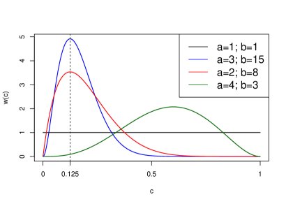
We illustrate the interpretations of the weight functions with Beta distributions. Figure 1 displays the density functions of several Beta distributions. As noted earlier, the Brier score uses the uniform distribution, , as the weight function. If we believe that for the majority of the population, the cost of false negative (i.e., in Table 1) is generally larger than the cost of false positive (i.e., ), we may choose or and not choose . and share a common mode of 1/8, representing two populations; both populations have a significant concentration of individuals with cost ratios close to . Two possible interpretations regard the difference between and . First, we may believe that better characterizes a more homogeneous population with less variable cost ratios. Taking the cancer surgery example discussed earlier as a hypothetical example, a population of patients with a similar age is expected to be more homogeneous in terms of the cost ratio. As an alternative interpretation, we may choose because we are not sure about the cost ratios in the population and are reluctant to put too much weight on a certain region. If we are certain that everyone in the population has the same cost ratio (e.g., ), we may choose a point mass function at 0.125 as , which results in or corresponding net benefit measures to assess the clinical utility. The exact choice of the weight function is not necessary, and we will show using a real data example in Section 5.2 that and give consistent rankings different from and , which illustrate a specification of the weight function broadly consistent with clinical utility would be sufficient in practice.
There are some similarities between choosing a sensible weight function and the informative prior elicitation in Bayesian analysis: 1) a simple distribution is chosen to represent the best knowledge about the population, with parameters often chosen by vague heuristics; 2) some sensitivity analyses by varying the parameters are helpful to assess the robustness of results. The difference is that, unlike Bayesian analysis, the distribution of the optimal cutoff or cost ratio is not the goal for inference. The distribution relies on the information intrinsic to the clinical or scientific problem but is usually external to the dataset at hand. Tsalatsanis et al., (2010) proposed an elicitation process for a single optimal risk cutoff in the context of the decision curve analysis. We can adopt their process to formally elicit the distribution of risk cutoff, and it is briefly described as follows: 1) educate physicians with the risk-based decision framework. Tsalatsanis et al., (2010) may help in this step; 2) present the physicians with patients from a real or hypothetical dataset with key covariates (e.g., age) and risk estimates that are representative of the population; 3) ask the physicians to make a treatment decision for each patient; 4) the decisions paired with the risk estimates can be used to construct the cutoff distribution.
Our proposal should not be confused with a different version of the weighted Brier score proposed in Gerds et al., (2008):
where and are chosen to assign different weights for cases and controls. This way of assigning weights is not coherent with the framework described in Section 2; hence, it is harder to specify or interpret. In contrast, our proposed weighted Brier score stemmed from the Schervish representation and quantifies the clinical utility within the risk-based decision framework.
Based on i.i.d. copies of validation data (, ) from a cohort study, the weighted Brier score can be empirically evaluated:
| (14) |
where , and are the cumulative density function (CDF), the 1st incomplete moment function and the 1st moment of the weight function , respectively.
Pfeiffer and Gail, (2020) considered a scenario in which the risk model is well-calibrated (i.e., ). Under this scenario, we have an alternative estimator, . The asymptotic distributions of and are derived in the Appendix. In line with the results from Pfeiffer and Gail, (2020) on estimating the net benefit, is more efficient than under the well-calibration assumption based on the asymptotic variance. One can follow the techniques described in Marsh et al., (2020) for the estimation and inference of in a (matched) case-control study.
4.2 Decomposition of the weighted Brier score and standardization
The Brier score assesses the overall prediction performance. Murphy’s decomposition of the Brier score (Murphy,, 1973) explicitly demonstrates that the Brier score inherently measures calibration and discrimination. Based on the recent work on the generalization of Murphy’s decomposition (Bröcker,, 2009; Siegert,, 2017), we decompose the weighted Brier score into calibration and discrimination components to better understand the impact of weighting. Before generalizing decomposition to the weighted Brier score, we first review the classic result of Murphy’s decomposition.
Murphy’s decomposition involves grouping in a similar way as the construction of the Hosmer–Lemeshow test (Hosmer and Lemesbow,, 1980) (e.g., forming groups by deciles of ). Suppose we divide the samples into groups, and and are the sample average of the observed event rate and the predicted risk within the group, respectively; is the total sample size of the group. The Brier score can be decomposed as:
The decomposition is exact when the predicted risk is discrete (e.g., ), and the arbitrary grouping for the continuous predicted risk results in a minimal discrepancy hence the approximation is usually sufficient enough in practical applications. We adopt the terminology from Dimitriadis et al., (2021) to name the three components the miscalibration component (), the discrimination component (), and the uncertainty component (). In some literature, the first two terms are also known as the reliability component () and the resolution component (), respectively.
quantifies the difference between the expected event rate () and the observed event rate (). is also known as the recalibrated risk in the group. measures the differences between the recalibrated risks and the overall event rate () for the discrimination ability. A highly discriminative risk prediction model would have largely different from , which leads to a higher . If we make an uninformative prediction for each observation by using the overall event rate (), would be 0 ( would be 0 as well). measures the inherent difficulties in predicting a binary outcome.
Bröcker, (2009) generalized Murphy’s decomposition of the Brier score to any strictly proper scoring rule. We apply the methodology to the weighted Brier score. In particular, we can decompose the expected weighted Brier score as follows:
| (15) |
where is the recalibrated risk; is known as divergence; is the cost-weighted misclassification loss function with probabilities as the input for both arguments. One can verify that when the weight function, , is the PDF of uniform distribution over (0,1), we have and ; thus, the classical Murphy’s decomposition of the Brier score is a special case.
The decomposition suggests that the weighted Brier score also measures discrimination and calibration; compared with the Brier score, by construction, each component additionally takes the clinical utility into account, which is numerically demonstrated in Section 5.
Kattan and Gerds, (2018) promoted a scaled version of the Brier scores, , to measure the prediction performance, termed IPA. Arguably, the IPA is more interpretable because it ranges from 0 to 100% corresponding to a lower bound from an uninformative prediction and an upper bound from a perfect prediction . Using the decomposition components, we write . Similarly, we can define the scaled and weighted Brier score by arranging the corresponding weighted decomposition components: .
4.3 Some related measures: the measure and Spiegelhalter’s Z-statistic
In this subsection, we make connections between the weighted Brier score and some other previously proposed measures for evaluating a risk prediction model, in particular, the measure (Hand,, 2009, 2010) and Spiegelhalter’s Z-statistic (Spiegelhalter,, 1986; Rufibach,, 2010). Interestingly, these two measures consider two aspects of a risk prediction model, discrimination and calibration, separately.
These connections demonstrate that the formulation of the weighted Brier score is not only useful in the application of risk prediction assessment but also insightful for statistical methodology development, and are summarized as a remark at the end of this subsection.
4.3.1 The measure
Hand, (2009, 2010) proposed a summary measure, called the measure, to quantify the discrimination ability for predicting the binary outcome in a validation dataset. The construction of the measure shares the same spirit as the risk-based decision framework discussed in Section 2 in terms of choosing an optimal cutoff to balance different cost trade-offs; hence, the measure takes the clinical utility into account.
Instead of studying an estimated risk and a cutoff with a probability interpretation, Hand, (2009) considered a general real-valued score with a cutoff in the prediction problem. Similar to the definition of in Equation (9), Hand, (2009) considered an overall cost of binary decision as:
| (16) |
where and are costs of false negatives and false positives; because only the relative magnitude of the costs matters, one may replace and with hence the proportional sign appears in (16). and are the CDFs of among controls and cases. Through differentiation, one can note that an optimal cutoff to minimize must satisfy the following equality:
| (17) |
where and are the PDFs of among controls and cases. That is, , assuming that function is invertible. See Hand, (2009) for a relaxation in this invertible assumption. Note that is also known as the risk score, and the above discussion is in line with the optimality of the risk score (McIntosh and Pepe,, 2002).
Hand, (2009) showed that the AUC can be rewritten as:
where .
This implies that if we choose the cutoff optimally, the AUC is a function of a weighted average of the overall cost (), and the weight is a function of the disease prevalence () and the PDFs of among cases and controls. In essence, the derivation of involves changing of variable from the scale to the risk cutoff scale . Recall that the cutoff is key in the risk-based decision framework from Section 2. The challenge in interpreting is consistent with the clinical irrelevance in summarizing the ROC by integrating uniformly over . The clinical irrelevance of AUC motivates some notions of weighted AUC, which place weights on . The partial AUC is a special case of this type of weighted AUC (Pepe,, 2003; Li and Fine,, 2010).
Instead of having the weight function depend on the distribution of or placing weights on scale, Hand, (2010) suggested that one should place weights on the risk cutoff scale according to the costs trade-offs specific to the classification problem of interest, and define the weighted averaged cost as . The choice and interpretation of coincide with the construction of the weighted Brier score in Section 4.1.
Furthermore, if the continuous score () is a well-calibrated risk estimate, the weighted average cost () equals the expected weighted Brier score. To show this equality, note that if (i.e., well-calibrated), is the identity function hence pointwise; integrating with the same weight, , we have .
Hand, (2009) defined the measure by a standardization step: . When the distributions of are equal in cases and controls (i.e., ), , which is identical to the uncertainty component () from the decomposition of the weighted Brier score. Therefore, when is a well-calibrated risk estimate, the H measure equals the expectation of the scaled weighted Brier score (i.e., ).
In some sense, the measure and the scaled weighted Brier score are special cases of each other. The measure does not restrict the prediction score to a risk estimate; when the score is a risk estimate, the weighted Brier score assesses the score with or without miscalibration, and in a special case of well-calibration, the scaled weighted Brier score reduces to the measure.
4.3.2 Spiegelhalter’s Z-statistic
In this subsection, we extend the idea of weighting to Spiegelhalter’s Z-statistic to emphasize the assessment of miscalibration in certain risk cutoff regions that are more relevant to clinical decision-making.
Spiegelhalter’s Z-statistic is based on a simple decomposition of the Brier score (Rufibach,, 2010):
| (18) |
Under the well-calibration assumption (i.e., ), the first summand has expectation 0 conditional on , and we have an extra term: . To exploit this fact, Spiegelhalter, (1986) constructed a Z-statistic that is approximately standard normal under the well-calibration assumption:
| (19) |
where is the variance under the well-calibration assumption.
Spiegelhalter’s Z-statistic has been implemented in STATA (Stata et al.,, 2015) and a popular r-package rms (Harrell Jr,, 2015), and has some applications in the risk prediction research to assess calibration (e.g., Walsh et al.,, 2017). Huang et al., (2020) suggested that Spiegelhalter’s Z-statistic is not intuitive; thus, it is not widely used in practice compared to the Hosmer–Lemeshow statistic and the calibration plot. It is intuitive to assess the regions of miscalibration on the risk spectrum from the calibration plot or each summand in the Hosmer–Lemeshow statistic. On the contrary, Spiegelhalter’s Z-statistic assesses the calibration in a global sense, which is inherited from the Brier score as an overall summary. To alleviate this shortcoming, we can construct a weighted Spiegelhalter’s Z-statistic stemming from the weighted Brier score. We can adopt the notations from Section 4.2 to rewrite a general decomposition of (18) as:
| (20) |
Following the similar construction for Spiegelhalter’s Z-statistic, we can define a weighted version:
| (21) |
where is the square root of the estimated variance of under the null hypothesis of well-calibration (see Appendix for details). It is easy to verify that when is the uniform distribution over (0,1), Equations (18) and (19) are special cases of (20) and (21), respectively.
Remark.
The purpose of the discussion on the weighted Spiegelhalter’s Z-statistic as well as the measure is to show how ideas of the weighted Brier score can be interesting to researchers who focus on methodological development. For the weighted Brier score, the wide adoption of the measure in the machine learning community additionally validates the proposed weighting method. The lack of calibration in the measure coincides with over-emphasis on the AUC and relatively little attention to calibration, which is referred to as ‘the Achilles heel of predictive analytics’ (Van Calster et al.,, 2019). On the other hand, some researchers may simply equate the Brier score with calibration, which is incorrect because of the extra term in the decomposition of Spiegelhalter’s Z-statistic (Rufibach,, 2010). The swift construction of the weighted Spiegelhalter’s Z-statistic highlights the promising possibilities for novel methods that emerge from a deeper understanding of the Brier score. Indeed, as researchers who are interested in methodological development, we appreciate the elegant and practically meaningful mathematical structures that lie beneath the deceptively simple and familiar Brier score.
5 Numerical examples
In this section, we use various numerical examples to illustrate the merits of the weighted Brier score for comparing different risk models in a validation dataset. For the first part, we present two quite artificial sets of examples (Set A and Set B) with an arbitrarily large sample size () to clearly demonstrate the impact of weighting on the weighted Brier score via its and components. In the second part, we aim to demonstrate the weighted Brier score as a useful overall summary measure. We achieve this aim using a numerical example based on a real dataset with some simulated variables to mimic a potential dilemma in practice: comparing two risk prediction models when one model only outperforms the other model in discrimination or calibration but does not dominate both aspects simultaneously. Hereafter, we use to denote a weighted Brier score with the weight function from . In each example, multiple emphasized on a similar risk region are chosen as a sensitivity analysis.
5.1 Demonstration on the impact of weighting on and
5.1.1 Set A: the impact on
In the first set, we generate three models with the same AUC value, but only one model is the best in this simulated scenario. The binary outcome () is generated as a Bernoulli variable with . Among cases (), in Model 1, and in Model 2. Among controls (), for both Model 1 and Model 2. Via the Bayes formula, we can calculate the predicted risk, , denoted as and , respectively, for Model 1 and Model 2. The predicted risk for Model 3, , is generated based on as:
Construction of Model 3 with over-fitted risk is similar to the examples from Hilden and Gerds, (2014) and Pepe et al., (2015) demonstrating the non-properness of IDI and NRI.
| Model 1 | Model 2 | Model 3 | |
|---|---|---|---|
| AUC | 0.831 | 0.831 | 0.831 |
| (0.3) | 0.327 | 0.384 | 0.384 |
| IPA | 0.372 | 0.372 | 0.289 |
| (1,1) | 0.078 | 0.078 | 0.089 |
| 0.000 | 0.000 | 0.010 | |
| 0.046 | 0.046 | 0.046 | |
| (2,5) | 0.096 | 0.073 | 0.076 |
| 0.000 | 0.000 | 0.003 | |
| 0.036 | 0.059 | 0.059 | |
| (4,8) | 0.110 | 0.084 | 0.087 |
| 0.000 | 0.000 | 0.002 | |
| 0.048 | 0.074 | 0.074 |
-
•
(0.3): the opt-in net benefit with cutoff at 0.3; : a weighted Brier score with the weight function from ; (): the miscalibration (discrimination) component of the weighted Brier score.
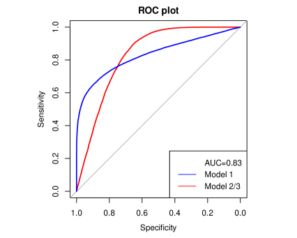
Based on the classic result of binormal ROC (Pepe,, 2003), Model 1 and Model 2 have the same AUC, and due to the monotonic transformation, Model 3 and Model 2 have the identical ROC as shown in Figure 2. Similar to the AUC, the unweighted Brier score () or its scaled version, IPA (Kattan and Gerds,, 2018), cannot distinguish Model 1 and Model 2 as shown in Table 2. In clinical scenarios where a majority of the population chooses low-risk cutoffs (i.e., not treating a case is worse than treating a control), compared with Model 1, Model 2 has better clinical utility as demonstrated by the smaller values in the weighted Brier scores ( or ) with additional weights placed on the lower cutoffs. The smaller weighted Brier score results from a higher in Model 2, which suggests better discrimination for these specific clinical scenarios. Loosely speaking, one may visualize that the additional weights are put on the high-sensitivity region on the top right of the ROC plot (more precisely, the low-risk region on the absolute risk scale). Because Model 1 and Model 2 are perfectly calibrated due to the correct model specification via the Bayes formula, any weight function would lead to .
The comparison between Model 2 and Model 3 aims to demonstrate the non-strictness of the net benefit measures. Note that (0.3) cannot distinguish an over-fitted/miscalibrated model (Model 3) from its perfectly calibrated counterpart (Model 2). On the other hand, as a strictly proper scoring rule, the weighted Brier scores pick Model 2 as the best model.
5.1.2 Set B: the impact on
In Set A, by comparing two models with the same AUC but crossed ROC, we demonstrate that the weighted Brier score can pick up the best model in terms of discrimination for the specific cost trade-offs, whereas the unweighted Brier score cannot. In Set B, we construct an example that the unweighted Brier score cannot distinguish two models with miscalibration in the lower or higher risk regions, but the weighted Brier score can meaningfully distinguish the miscalibration that matters the most for clinical decision-making.
The binary outcome () is again generated as a Bernoulli variable with . For the True Model, among cases (), ; among controls (), . Again, via the Bayes formula, the predicted risk of the True model, , can be calculated. Two miscalibrated models are constructed based on the True Model. In particular, an over-fitted in high-risk region (OH) model is constructed as:
An over-fitted in low-risk region (OL) model is constructed as:
Again, we consider the scenarios that the risk cutoff for the majority of the population is smaller than 0.5. In these scenarios, we expect the miscalibration in the lower-risk region to have a more negative impact on the decision-making and, hence, the clinical utility of the model. Indeed, as shown in Table 3, the weighted Brier scores with more weights in the lower risk region ( or ) are lower in the OH model than those in the OL model, indicating inferior clinical utility of the OL model. More specifically, the difference in is due to the impact of weighting on ; as expected, the three models share the same regardless of the weights. Due to the symmetry in the data-generating mechanism, the unweighted Brier score () or its scaled version, IPA, shows the same level of miscalibration in terms of .
| True Model | OH Model | OL Model | |
|---|---|---|---|
| IPA | 0.2032 | 0.1452 | 0.1452 |
| (1,1) | 0.0996 | 0.1068 | 0.1068 |
| 0.0000 | 0.0072 | 0.0072 | |
| 0.0250 | 0.0250 | 0.0250 | |
| (2,5) | 0.1068 | 0.1077 | 0.1227 |
| 0.0000 | 0.0009 | 0.0158 | |
| 0.0257 | 0.0257 | 0.0257 | |
| (4,8) | 0.1239 | 0.1245 | 0.1408 |
| 0.0000 | 0.0006 | 0.0168 | |
| 0.0345 | 0.0345 | 0.0345 |
-
•
: a weighted Brier score with the weight function from ; (): the miscalibration (discrimination) component of the weighted Brier score.
5.2 A numerical example: the weighted Brier score as a useful overall summary
Based on Prostate Cancer Active Surveillance Study (PASS) data, we demonstrate the weighted Brier score as a useful overall summary in a difficult scenario: some models are better in terms of discrimination while the other models are better in terms of calibration. We also keep in mind clinical utility when evaluating rival models. To create such a scenario, we simulate some variables, which are described after introducing the clinical problem and the dataset in the PASS.
In the PASS, risk models are built to predict high-grade cancer at each biopsy with a set of clinical covariates (Lin et al.,, 2017). The clinical application of these risk models is to inform a risk-based decision on whether to opt out of a surveillance biopsy. A patient with a low risk of high-grade cancer for the next surveillance biopsy may skip the biopsy, which is invasive and may cause infection. However, skipping a surveillance biopsy may miss a progressive cancer. In general, missing a progressive cancer is several times more costly than an unnecessary invasive biopsy.
Our goal is to compare rival risk models for the clinical application that relies on the framework described in Section 2. Suppose the physicians agree that the cost of missing progressive cancer for a typical patient in this population () is about seven times more than the cost of an unnecessary invasive biopsy (), which results in . Thus, the net benefit, , is considered as a summary measure. To acknowledge the heterogeneity in the cost-benefit assessment, each patient in the population may consider a different risk threshold. Thus, we also consider several weight Brier scores (i.e., and ). Note that the modes of and are both 1/8, and the percentiles of and are approximately 0.43 and 0.33, respectively. That is, very few patients would consider a risk threshold higher than 0.4. Two weighted Brier scores are chosen here as a sensitivity analysis. Just for illustrative purposes, we also consider an irrational choice of weight, , which places the majority of its mass on the cutoffs greater than 0.5 (Figure 1), suggesting an unlikely patient’s cost-benefit assessment that the cost of an unnecessary invasive biopsy is greater than the cost of missing progressive cancer. In addition, we also consider the AUC, the mean calibration (Van Calster et al.,, 2019), the unweighted Brier score (), and its scaled version, IPA (Kattan and Gerds,, 2018).
The dataset consists of 3384 active surveillance biopsies from 1612 patients. We randomly split the patients into a training set and a validation set in a 1:1 ratio. In the training set, we fit a logistic regression model with high-grade cancer as the binary outcome (i.e., for Gleason Group 2 or higher) and a set of clinical variables as the covariates, including prostate size, PSA, prior max cores ratio, number of prior negative biopsies, BMI, time since diagnosis and age.
Based on the dataset, we simulate some variables in the context of outcome misclassification to highlight the potential dilemma when evaluating competing models. The biopsies and their observed results () in the data were obtained from the leading academic hospitals of the PASS sites. We consider some less accurate biopsy results from some hypothetical community clinics. We simulate two sets of inaccurate results with different levels of accuracy for comparison purposes. In particular, we simulate with and ; with and . The event rates of , , and are 0.23, 0.2, and 0.31, respectively. The logistic regression with the same set of covariates is fitted with or as the outcomes. We call the logistic regressions with , , and as Model Y, Model S1, and Model S2 respectively.
To make this example even more illustrative, we simulate an additional variable in cases and in controls. We fit another logistic regression model with as the outcome and the same set of clinical variables plus the new variable as the covariates. We denote this model as Model S2+. We expect Model S2+ to have a higher AUC due to the additional predictor but less calibrated than Model Y due to the errors in .
| Model Y | Model S1 | Model S2 | Model S2+ | |
|---|---|---|---|---|
| AUC | 0.76 (0.73,0.79) | 0.76 (0.73,0.79) | 0.76 (0.73,0.79) | 0.78 (0.75,0.81) |
| 1 (0.95,1.1) | 1.1 (1,1.2) | 0.73 (0.67,0.8) | 0.73 (0.67,0.8) | |
| 0.076 (0.07,0.082) | 0.077 (0.071,0.084) | 0.08 (0.076,0.085) | 0.078 (0.074,0.083) | |
| IPA | 0.16 (0.12,0.19) | 0.14 (0.11,0.16) | 0.11 (0.068,0.14) | 0.13 (0.087,0.16) |
| 0.088 (0.081,0.094) | 0.091 (0.085,0.096) | 0.1 (0.097,0.1) | 0.096 (0.092,0.1) | |
| 0.084 (0.077,0.09) | 0.087 (0.081,0.092) | 0.099 (0.096,0.1) | 0.095 (0.091,0.098) | |
| 0.089 (0.081,0.098) | 0.091 (0.082,0.1) | 0.091 (0.084,0.098) | 0.09 (0.083,0.097) | |
| 0.16 (0.099,0.23) | 0.1 (0.047,0.15) | 0.013 (0.0010,0.024) | 0.037 (0.023,0.049) |
-
•
: a weighted Brier score with the weight function from ; : observed event rate over expected average risk, i.e., the mean calibration (Van Calster et al.,, 2019)
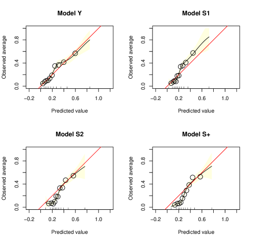
The predicted risks of high-grade cancer from each model are evaluated in the validation set with as the outcome. The summary measures are presented in Table 4. We construct the confidence intervals using the bootstrap approach with each individual patient as the resampling unit to account for the correlation. Model Y, Model S1, and Model S2 have almost identical AUC because the non-differential errors in the binary outcome would not change the rank of predicted risks (Neuhaus,, 1999). Due to the errors in the outcome, Model S1, Model S2, and Model S2+ are not well calibrated, the mean calibration, , in Table 4. As shown in Figure 3, Model S1 is less calibrated and tends to underestimate the risk in the high-risk region, and Model S2 and Model S2+ are less calibrated and tend to overestimate the risk in the low-risk region.
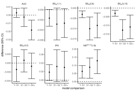
We visualize some selected pairwise comparisons among four models in Figure 4. Overall, , and clearly indicate that Model Y is better than Model S1 or Model S2+; Model S1 is better than Model S2. Although and IPA generally indicate similar conclusions, their confidence intervals cover 0.
Specifically, with more weight placed on the low-risk region (e.g., with instead of , the increasingly lower value in in Model S1 compared with Model S2 suggests stronger evidence for the superiority of Model S1 over Model S2. This is expected because the heavier weight in the low-risk region amplifies the poorer calibration of Model S2 in the region, which significantly impacts the decision-making with the cost trade-off consideration. On the other hand, the positive difference in reflects a better calibration of Model S2 on the higher-risk region although the difference is much more subtle due to the small portion of patients in the high-risk region. As noted earlier, this comparison based on is irrational and not clinically meaningful when most of the cutoffs lay in the lower-risk region.
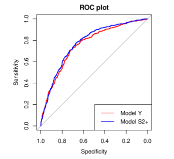
Compared with Model Y, Model S2+ is better in discrimination in terms of the ROC (Figure 5) but is less calibrated (Figure 3), so we are in a dilemma of choosing a better model among these two models. The lower weighted Brier scores suggest that overall, Model Y is a better model in the context of the intended clinical application of the risk prediction model and cost trade-off in the patient population. This comparison highlights the importance of calibration for risk-based decisions, in particular in the relevant risk region, which may overshadow a good discriminatory ability.
6 Discussion
In this paper, we present a new clinically relevant summary measure for risk prediction models, namely, the weighted Brier score. The classic Brier score is recognized in the field as a useful overall summary measure for both discrimination and calibration but faces criticism for its inability to measure the clinical utility (Assel et al.,, 2017). We analytically show this caveat of the classic Brier score and further construct the weighted Brier score that can meaningfully measure the clinical utility. The weighted Brier score shares the same decision-theoretic framework as the popular summary measure of net benefit. Specifying a distribution on the cutoffs for is more natural for the population-level summary measure than requiring a single cutoff for the whole population, as the population of interest is often heterogeneous in its cost-benefit profile.
The decision-theoretic framework involves a priori and vague knowledge about a particular application external to the data at hand. When equipped with rationally selected weights and coupled with sensitivity analyses as demonstrated in the numerical examples, the weighted Brier score offers initial assessment and valuable information on the relative clinical utility of multiple risk prediction models. This knowledge facilitates the selection of a handful of promising models for further evaluation, motivating subsequent studies with longitudinal follow-up to objectively gather data regarding cost-effectiveness.
Our work utilizes many results from the study of proper scoring rules, which is most familiar to the weather forecast community. We additionally connect our work to the measure proposed by Hand, (2009), which has been widely cited and utilized across various applications in the machine learning field, such as benchmarking credit scoring systems in finance (Lessmann et al.,, 2015). We hope this work also stimulates future methodology development in the field of medical risk prediction.
One interesting direction is on the evaluation of prediction models for time-to-event outcomes, particularly in the context of flexible machine learning algorithms with their output being individualized survival curves (e.g., Haider et al.,, 2020; Rindt et al.,, 2022; Qi et al.,, 2023). Along with adequate handling of censoring, clinically meaningful characterization of calibration, discrimination, and clinical utility for the prediction of time-to-event outcome warrants follow-up research in the lens of proper scoring rules. These predictions are probabilistic forecasting (Gneiting and Katzfuss,, 2014), and there has been active research in this area (Ehm et al.,, 2016; Gneiting et al.,, 2023). Such follow-up research may generalize the metrics related to commonly studied t-year risks and the concordance probability (Heagerty and Zheng,, 2005) or its recent variants (Blanche et al.,, 2019; Devlin et al.,, 2020; Devlin and Heller,, 2021).
Acknowledgments
The work is supported by grants R01 CA236558 and U24 CA086368 awarded by the National Institutes of Health.
References
- Assel et al., (2017) Assel, M., Sjoberg, D. D., and Vickers, A. J. (2017). The brier score does not evaluate the clinical utility of diagnostic tests or prediction models. Diagnostic and prognostic research, 1(1):1–7.
- Blanche et al., (2019) Blanche, P., Kattan, M. W., and Gerds, T. A. (2019). The c-index is not proper for the evaluation of-year predicted risks. Biostatistics, 20(2):347–357.
- Brier, (1950) Brier, G. W. (1950). Verification of forecasts expressed in terms of probability. Monthly weather review, 78(1):1–3.
- Bröcker, (2009) Bröcker, J. (2009). Reliability, sufficiency, and the decomposition of proper scores. Quarterly Journal of the Royal Meteorological Society: A journal of the atmospheric sciences, applied meteorology and physical oceanography, 135(643):1512–1519.
- Devlin et al., (2020) Devlin, S. M., Gönen, M., and Heller, G. (2020). Measuring the temporal prognostic utility of a baseline risk score. Lifetime data analysis, 26:856–871.
- Devlin and Heller, (2021) Devlin, S. M. and Heller, G. (2021). Concordance probability as a meaningful contrast across disparate survival times. Statistical methods in medical research, 30(3):816–825.
- Dimitriadis et al., (2021) Dimitriadis, T., Gneiting, T., and Jordan, A. I. (2021). Stable reliability diagrams for probabilistic classifiers. Proceedings of the National Academy of Sciences, 118(8).
- Ehm et al., (2016) Ehm, W., Gneiting, T., Jordan, A., and Krüger, F. (2016). Of quantiles and expectiles: consistent scoring functions, choquet representations and forecast rankings. Journal of the Royal Statistical Society Series B: Statistical Methodology, 78(3):505–562.
- Elkan, (2001) Elkan, C. (2001). The foundations of cost-sensitive learning. In International joint conference on artificial intelligence, volume 17, pages 973–978.
- Gail and Pfeiffer, (2005) Gail, M. H. and Pfeiffer, R. M. (2005). On criteria for evaluating models of absolute risk. Biostatistics, 6(2):227–239.
- Gerds et al., (2008) Gerds, T. A., Cai, T., and Schumacher, M. (2008). The performance of risk prediction models. Biometrical Journal: Journal of Mathematical Methods in Biosciences, 50(4):457–479.
- Gneiting and Katzfuss, (2014) Gneiting, T. and Katzfuss, M. (2014). Probabilistic forecasting. Annual Review of Statistics and Its Application, 1:125–151.
- Gneiting and Raftery, (2007) Gneiting, T. and Raftery, A. E. (2007). Strictly proper scoring rules, prediction, and estimation. Journal of the American statistical Association, 102(477):359–378.
- Gneiting et al., (2023) Gneiting, T., Wolffram, D., Resin, J., Kraus, K., Bracher, J., Dimitriadis, T., Hagenmeyer, V., Jordan, A. I., Lerch, S., Phipps, K., et al. (2023). Model diagnostics and forecast evaluation for quantiles. Annual Review of Statistics and Its Application, 10:597–621.
- Haider et al., (2020) Haider, H., Hoehn, B., Davis, S., and Greiner, R. (2020). Effective ways to build and evaluate individual survival distributions. The Journal of Machine Learning Research, 21(1):3289–3351.
- Hand, (2009) Hand, D. J. (2009). Measuring classifier performance: a coherent alternative to the area under the roc curve. Machine learning, 77(1):103–123.
- Hand, (2010) Hand, D. J. (2010). Evaluating diagnostic tests: the area under the roc curve and the balance of errors. Statistics in medicine, 29(14):1502–1510.
- Harrell Jr, (2015) Harrell Jr, F. E. (2015). Regression modeling strategies: with applications to linear models, logistic and ordinal regression, and survival analysis. springer.
- Heagerty and Zheng, (2005) Heagerty, P. J. and Zheng, Y. (2005). Survival model predictive accuracy and roc curves. Biometrics, 61(1):92–105.
- Hilden and Gerds, (2014) Hilden, J. and Gerds, T. A. (2014). A note on the evaluation of novel biomarkers: do not rely on integrated discrimination improvement and net reclassification index. Statistics in medicine, 33(19):3405–3414.
- Hosmer and Lemesbow, (1980) Hosmer, D. W. and Lemesbow, S. (1980). Goodness of fit tests for the multiple logistic regression model. Communications in statistics-Theory and Methods, 9(10):1043–1069.
- Huang et al., (2020) Huang, Y., Li, W., Macheret, F., Gabriel, R. A., and Ohno-Machado, L. (2020). A tutorial on calibration measurements and calibration models for clinical prediction models. Journal of the American Medical Informatics Association, 27(4):621–633.
- Kattan and Gerds, (2018) Kattan, M. W. and Gerds, T. A. (2018). The index of prediction accuracy: an intuitive measure useful for evaluating risk prediction models. Diagnostic and prognostic research, 2(1):1–7.
- Kerr et al., (2016) Kerr, K. F., Brown, M. D., Zhu, K., and Janes, H. (2016). Assessing the clinical impact of risk prediction models with decision curves: guidance for correct interpretation and appropriate use. Journal of Clinical Oncology, 34(21):2534.
- Lessmann et al., (2015) Lessmann, S., Baesens, B., Seow, H.-V., and Thomas, L. C. (2015). Benchmarking state-of-the-art classification algorithms for credit scoring: An update of research. European Journal of Operational Research, 247(1):124–136.
- Li and Fine, (2010) Li, J. and Fine, J. P. (2010). Weighted area under the receiver operating characteristic curve and its application to gene selection. Journal of the Royal Statistical Society: Series C (Applied Statistics), 59(4):673–692.
- Lin et al., (2017) Lin, D. W., Newcomb, L. F., Brown, M. D., Sjoberg, D. D., Dong, Y., Brooks, J. D., Carroll, P. R., Cooperberg, M., Dash, A., Ellis, W. J., et al. (2017). Evaluating the four kallikrein panel of the 4kscore for prediction of high-grade prostate cancer in men in the canary prostate active surveillance study. European urology, 72(3):448–454.
- Marsh et al., (2020) Marsh, T. L., Janes, H., and Pepe, M. S. (2020). Statistical inference for net benefit measures in biomarker validation studies. Biometrics, 76(3):843–852.
- McIntosh and Pepe, (2002) McIntosh, M. W. and Pepe, M. S. (2002). Combining several screening tests: optimality of the risk score. Biometrics, 58(3):657–664.
- Mitchell, (2019) Mitchell, K. (2019). Score decompositions in forecast verification. PhD thesis, University of Exeter.
- Murphy, (1973) Murphy, A. H. (1973). A new vector partition of the probability score. Journal of Applied Meteorology and Climatology, 12(4):595–600.
- Neuhaus, (1999) Neuhaus, J. M. (1999). Bias and efficiency loss due to misclassified responses in binary regression. Biometrika, 86(4):843–855.
- Pauker and Kassirer, (1975) Pauker, S. G. and Kassirer, J. P. (1975). Therapeutic decision making: a cost-benefit analysis. New England Journal of Medicine, 293(5):229–234.
- Pepe, (2003) Pepe, M. S. (2003). The statistical evaluation of medical tests for classification and prediction. Medicine.
- Pepe et al., (2015) Pepe, M. S., Fan, J., Feng, Z., Gerds, T., and Hilden, J. (2015). The net reclassification index (nri): a misleading measure of prediction improvement even with independent test data sets. Statistics in biosciences, 7(2):282–295.
- Pessach and Shmueli, (2022) Pessach, D. and Shmueli, E. (2022). A review on fairness in machine learning. ACM Computing Surveys (CSUR), 55(3):1–44.
- Pfeiffer and Gail, (2017) Pfeiffer, R. M. and Gail, M. H. (2017). Absolute risk: methods and applications in clinical management and public health. CRC Press.
- Pfeiffer and Gail, (2020) Pfeiffer, R. M. and Gail, M. H. (2020). Estimating the decision curve and its precision from three study designs. Biometrical Journal, 62(3):764–776.
- Qi et al., (2023) Qi, S.-a., Kumar, N., Farrokh, M., Sun, W., Kuan, L.-H., Ranganath, R., Henao, R., and Greiner, R. (2023). An effective meaningful way to evaluate survival models. arXiv preprint arXiv:2306.01196.
- Reid and Williamson, (2011) Reid, M. and Williamson, R. (2011). Information, divergence and risk for binary experiments.
- Reid and Williamson, (2010) Reid, M. D. and Williamson, R. C. (2010). Composite binary losses. The Journal of Machine Learning Research, 11:2387–2422.
- Rindt et al., (2022) Rindt, D., Hu, R., Steinsaltz, D., and Sejdinovic, D. (2022). Survival regression with proper scoring rules and monotonic neural networks. In Camps-Valls, G., Ruiz, F. J. R., and Valera, I., editors, Proceedings of The 25th International Conference on Artificial Intelligence and Statistics, volume 151 of Proceedings of Machine Learning Research, pages 1190–1205. PMLR.
- Rufibach, (2010) Rufibach, K. (2010). Use of brier score to assess binary predictions. Journal of clinical epidemiology, 63(8):938–939.
- Sande et al., (2020) Sande, S. Z., Li, J., D’Agostino, R., Yin Wong, T., and Cheng, C.-Y. (2020). Statistical inference for decision curve analysis, with applications to cataract diagnosis. Statistics in Medicine, 39(22):2980–3002.
- Schervish, (1989) Schervish, M. J. (1989). A general method for comparing probability assessors. The annals of statistics, 17(4):1856–1879.
- Siegert, (2017) Siegert, S. (2017). Simplifying and generalising murphy’s brier score decomposition. Quarterly Journal of the Royal Meteorological Society, 143(703):1178–1183.
- Spiegelhalter, (1986) Spiegelhalter, D. J. (1986). Probabilistic prediction in patient management and clinical trials. Statistics in medicine, 5(5):421–433.
- Stata et al., (2015) Stata, A., Publication, P., and Lp, S. (2015). Stata base reference manual release 14.
- Steyerberg et al., (2010) Steyerberg, E. W., Vickers, A. J., Cook, N. R., Gerds, T., Gonen, M., Obuchowski, N., Pencina, M. J., and Kattan, M. W. (2010). Assessing the performance of prediction models: a framework for some traditional and novel measures. Epidemiology (Cambridge, Mass.), 21(1):128.
- Tsalatsanis et al., (2010) Tsalatsanis, A., Hozo, I., Vickers, A., and Djulbegovic, B. (2010). A regret theory approach to decision curve analysis: a novel method for eliciting decision makers’ preferences and decision-making. BMC medical informatics and decision making, 10(1):1–14.
- Van Calster et al., (2019) Van Calster, B., McLernon, D. J., Van Smeden, M., Wynants, L., and Steyerberg, E. W. (2019). Calibration: the achilles heel of predictive analytics. BMC medicine, 17(1):1–7.
- Vickers and Elkin, (2006) Vickers, A. J. and Elkin, E. B. (2006). Decision curve analysis: a novel method for evaluating prediction models. Medical Decision Making, 26(6):565–574.
- Walsh et al., (2017) Walsh, C. G., Sharman, K., and Hripcsak, G. (2017). Beyond discrimination: a comparison of calibration methods and clinical usefulness of predictive models of readmission risk. Journal of biomedical informatics, 76:9–18.
Appendix
Appendix A Asymptotic distributions of and
A.1
Denote and .
From the central limit theorem, we have
where
Note that we used , and .
Under the well-calibration assumption (i.e.,), we have
A.2
Under the well-calibration assumption, .
From the central limit theorem, we have
where
Make a comparison between the variances of and under the well-calibration assumption:
Note that for some ; thus for non-generative cases (i.e. is not constant 0 or 1).
Therefore, under the well-calibration assumption, is more efficient than .